The PMSM Machine EIE015 Power Electronics Lab Before the lab, look through the manual and make sure you are familiar with all parts! 1 Introduction In this lab modulation, current control, field weakening and speed control for a PMSM machine electric drive system will be studied. The control system for the lab is implemented with a graphical programming language called LabView and is executed in a CompactRIO which controls the power electronics and sample the feedback signals. The controller settings which decides in what way the CompactRIO should act is made on an interface implemented on a PC. 2 The equipment The data of the PMSM necessary for the torque control is presented below in table 3.1. This data is used to design the PIE current controller. Table 2.1 The PMSM control design data Measure Symbol Value Unit Nominal flux linkage of the PMSM Ψpm 0.16 Vs Stator inductance of the PMSM Lsx= Lsy 3 mH Stator resistance of the PMSM Rs 0.5 Ω The nominal current of the PMSM In 12 A The nominal voltage of the PMSM ULn 400 V Sample time Ts 1e‐4 s 2.1 The motor bench All motor control labs will be made with the same motor setup. It consists of two or three motors, an externally magnetized DC Machine, a Permanent Magnetized Synchronous Machine and on some stations also an asynchronous machine. They are all mechanically coupled to the same shaft and a positive torque is always accelerating the shaft in the same direction, independent of which motor the reference is fed to. The idea of the setup is to drive the common shaft with one of the machines and brake it with another. In this lab you will drive with the PMSM and later brake with the DC Machine by applying an external resistive load to its terminals. This means that the no load voltage of the DC Machine, that is
Transcript
The PMSM Machine EIE015 Power Electronics Lab
Before the lab, look through the manual and make sure you are familiar with all parts!
1 Introduction
In this lab modulation, current control, field weakening and speed control for a PMSM machine electric
drive system will be studied. The control system for the lab is implemented with a graphical
programming language called LabView and is executed in a CompactRIO which controls the power
electronics and sample the feedback signals. The controller settings which decides in what way the
CompactRIO should act is made on an interface implemented on a PC.
2 The equipment
The data of the PMSM necessary for the torque control is presented below in table 3.1. This data is
used to design the PIE current controller.
Table 2.1 The PMSM control design data
Measure Symbol Value Unit
Nominal flux linkage of the PMSM Ψpm 0.16 Vs
Stator inductance of the PMSM Lsx= Lsy 3 mH
Stator resistance of the PMSM Rs 0.5 Ω
The nominal current of the PMSM In 12 A
The nominal voltage of the PMSM ULn 400 V
Sample time Ts 1e‐4 s
2.1 The motor bench
All motor control labs will be made with the same motor setup. It consists of two or three motors, an
externally magnetized DC Machine, a Permanent Magnetized Synchronous Machine and on some
stations also an asynchronous machine. They are all mechanically coupled to the same shaft and a
positive torque is always accelerating the shaft in the same direction, independent of which motor the
reference is fed to.
The idea of the setup is to drive the common shaft with one of the machines and brake it with another.
In this lab you will drive with the PMSM and later brake with the DC Machine by applying an external
resistive load to its terminals. This means that the no load voltage of the DC Machine, that is
Lab: The PMSM 2
proportional to speed, will be applied to the external resistor and the braking power thus proportional
to speed squared and inversely proportional to resistance.
There is a resolver mounted on the shaft which provides the cRIO with feedback signals for instance
for the vector control of the PMSM or for speed control for instance.
3 The control system
3.1 The CompactRIO
The CompactRIO, cRIO, consists basically of three parts; a Field Programmable Gate Array, FPGA, a Real
Time system, RT, and the Inputs and Outputs, I/O.
3.2 FPGA
The FPGA is a programmable electrical circuit. This means that the program that has been written to it
actually is built in hardware with logical gates. From the programs point of view this means that every
part of it is executed simultaneously. The FPGA is connected to both the RT system and the I/O‐
modules. It therefore acts as the bridge between the I/O-modules and the RT system. It can also make
some or all of the signal processing, which will be utilized in this setup. Since the space on the FPGA is
limited it is important to choose what to implement on it. The characteristics of things that should be
implemented on the FPGA is that they need to execute fast, often and/or in parallel.
3.3 RT
The real time system consists of an industry PC and a Real Time operating system. Programs on the RT
system make things that do not have high demands on speed or tasks that are typical for a computer
like read and write to files, talk over Ethernet, display information and so on.
3.4 I/O
The cRIO is flexible unit where you can insert different I/O‐modules, the cRIO used in the labs can take
up to eight different modules. For example an eight channel TTL I/O is used to control the power
electronics and a fast, simultaneously sampling four channel AD module is used to sample time critical
signals, such as the current and the resolver signals.
3.5 Signal conditioning
Normally the I/O modules is intended to work with small signals, i.e. small voltages and currents. Since
the power electronics is working with larger signals it is necessary to have some signal conditioning
between them. This is done by a unit placed between the cRIO and the power electronics. The same
unit also excites and interprets the resolver and provides some useful measuring points.
3.6 The interface
The interface is mainly a tab‐based interface. The idea is to save space on the control panel and to only
show necessary controls, graphs, etc. Some of the control elements are always good to keep within
reach, such as the stop button or the DC‐link voltage. They are placed on upper part of the panel.
There are a number of boxes where you can enter variables; these are normally saved when you press
enter after entering them, even if you leave the tab. However some setting, reference generators for
example, are turned off when leaving a tab.
Lab: The PMSM 3
3.7 Setup tab
This tab contains several sub‐tabs which are not meant to be changed during the lab. Briefly the idea
is to set up the controller for different signal conditioning, motors, etc., and to do some underlying
tests.
Figure 1 The Setup Tab – Setting general parameters (do not change there during the lab)
Here you set the speed controller and current controller parameters, as well as a scaling factor for DC
link voltage measurement.
3.8 Voltage control
This option is not supposed to be used in the labs. It allows the user to enter a voltage reference to the
modulator. It is useful during tests as you can generate a PWM signal without any feedback signals.
Since the height of the carrier wave in the modulator is scaled with the DC link voltage it is possible for
a disturbance to propagate in to the system this way. Hence a variable hysteresis band is implemented
in the modulator, whose height is entered in volts in the modulator hysteresis band box. Normally the
current sampling is synchronized with the turning points of the carrier wave in the modulator, but
since there are delays, mainly in the power electronics, it is sometimes useful to apply a delay on the
sampling point. This delay is entered in the sampling delay box.
Lab: The PMSM 4
Figure 2 Tab to set output Voltage
3.9 Current control
Here you can choose if you want to tune the PI current controller or the tolerance band current
controller.
PI current control
The reference generator enables you to set a constant, sine or square wave reference with offset. The
dead beat parameters are calculated from the entered motor data, and a 1.0 setting on the slider
GAINS corresponds to those values (See the Setup tab).
Figure 3 PI based current control parameters
Lab: The PMSM 5
Tolerance band current control
This tab is very similar to the sampled current controller tab. There are two parameters to tune, the
inner and outer hysteresis bands as illustrated.
Figure 4 Tolerance band current control parameters
3.10 Modulation
In this tab you can try out the three different variants of modulation that are taught in the course.
Figure 5 The Modulation tab
Lab: The PMSM 6
3.11 Field Weakening
In this tab you can try out the effect of introducing a negative isx current as a field weakening effort.
Figure 6 The Field Weakening tab
3.12 Motor control / Speed Control
To control the speed of the DC machine a PI controller is used. It uses the reference created with the
generator and the feedback signal from the resolver to create a torque reference. The torque
reference is converted to a isy current reference and fed to the current controller that you choose.
Figure 7 Speed Controller
Lab: The PMSM 7
The PI control parameters are tuned with the sliders and the integrator could be reset with the reset
button.
3.13 Safety
Remember that the lab equipment involves voltage levels that are dangerous, especially at the
different terminals of the power electronic converter. Be careful!
The DC link voltage should always be the last thing to turn up during start up and always the first thing
to turn down during turn off.
Lab: The PMSM 8
4 Lab assignments
4.1 Getting started
1. Start the program National Instruments LabVIEW 2010, a Getting Started window will open.
2. Open the file C:\Labview\pmsm lab\20130213_pmsm_lab.lvproj. The Project Explorer for the
20130213_pmsm_lab project will open.
3. To open the control interface double click on PC_For_PMSM130226.vi.
4. Click on the run button in the upper left corner of the toolbar.
5. If everything works the icon of the run button changes and the control system is executed in the
cRIO system.
6. Make sure that everything else, such as the signal conditioning and the control system in the
power electronics is running.
4.2 Goal
The ambition with this lab is that you shall get “hands on” experience of the following:
• Controlling the three phase current with a 3‐phase bridge towards the RLE‐like rotor circuit of
a PMSM, both with a sampled current controller and a tolerance band controller. Study these
sections of the course material before you enter the lab.
• When working with the sampled current controller be aware of how I) the controller
parameter settings affect the response, II) how the voltage limitation affects the response and
finally, III) how “Anti Windup” helps in giving a stable control response with a limited output
voltage.
• Evaluating Field Weakening with the AC‐machine.
• Controlling Speed with the AC‐machine.
4.3 The Laboratory Exercises
The content of the laboratory exercises are divided into five parts:
1. Measuring the induced voltage of the PMSM and calculating the corresponding flux linkage.
2. Studying the different 3‐φ modulating references.
3. Adjusting the sampled vector current controller and the direct current controller for the PMSM.
4. Investigating field weakening.
5. Using Speed Control.
4.4 Induced Voltage
In this first part of the lab you will use the DC Machine to run the PMSM. This means the PMSM must
be disconnected from the 3‐φ VSC.
Make sure the red/yellow switch on the front panel of the PMSM VSC is set to 0.
Make sure the DC link voltage to minimum with the adjustable transformer on the table (The
output from the basement generator will not be exactly 0).
Connect the DC Machine Drive to the DC link using two short lab cables. The DC Machine VSC
should be turned off (with both the green switch and the red/yellow switch) through the whole
exercise. You will feed the DC Machine directly with the DC link voltage.
Lab: The PMSM 9
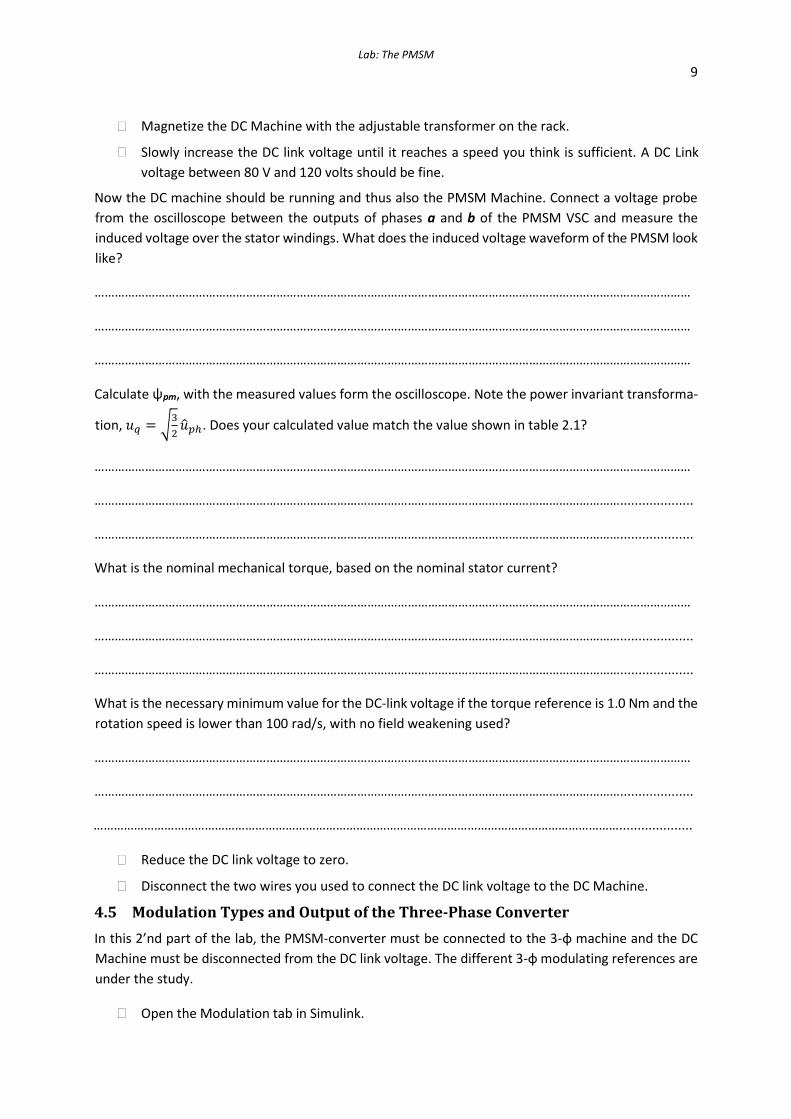
Magnetize the DC Machine with the adjustable transformer on the rack.
Slowly increase the DC link voltage until it reaches a speed you think is sufficient. A DC Link
voltage between 80 V and 120 volts should be fine.
Now the DC machine should be running and thus also the PMSM Machine. Connect a voltage probe
from the oscilloscope between the outputs of phases a and b of the PMSM VSC and measure the
induced voltage over the stator windings. What does the induced voltage waveform of the PMSM look