THE ROLE OF DEBT AND EQUITYFINANCING OVER THE BUSINESS

CYCLE

Francisco Covas and Wouter J. den Haan∗

November 14, 2005

Abstract

dKey Words: SJEL Classification: E

∗Covas, Bank of Canada, den Haan: London Business School and CEPR.

1

1 Introduction

The idea that changes in agency costs over the business cycle are importantto understand the severity and persistence of business cycles has obtaineda solid basis in economics. There are now several empirical and theoreticalpapers to support the basic idea. On the empirical side there is the classicpaper by Gertler and Gilchrist (1994) that shows that sales of small firmsare more sensitive to a monetary tightening than sales of large firms. On thetheoretical side there are numerous papers that can generate the net-worthchannel, that is, a deterioration in aggregate economic activity reduces firms’net worth, which aggravates the premium on external finance, which reduceslending and firm size, which in turn further slow down economic activity.

It is clear that incorporating agency problems into dynamic stochasticgeneral equilibrium (DSGE) models great improve the empirical predictionsof this class of models. But one shouldn’t overlook that these models havesome problems. First, in many models there is no default and in manymodels the default rate is procyclical. Both results are, of course, at oddswith the data. Second, the theoretical models typically assume the owner andmanager in the firm are the same agent and that the only type of externalfinance is debt finance. This means that in these models net worth onlyincreases through retained earnings. The traditional view is that empiricallythis is not a bad assumption. Recent studies1 document, however, that firmsissue equity frequently and that equity issuance is an important financingsource for increases in firm size. So although seasoned equity issues areindeed rare, the many other ways through which firms can issue equity arequantitatively very important. This means that the existing model is a badcharacterization of many firms in the modern economy and especially a badcharacterization of firms that are responsible for most of value added. Thethird deficiency of existing models is that a firm is simply an amount ofcapital and technology is such that the price of capital is equal to one (unitof consumption). Although, the introduction of adjustment costs allows forchanges in the price of capital the change in the value of the firm is still pinneddown by the technology to transform consumption into capital commodities.

In this paper we try to accomplish two things. In the first place we want todocument the cyclical behavior of default rates and financing sources (debt,retained earnings, and net-equity issuance). Not surprisingly we show that

1Fama and French (2005) and Frank and Goyal (2005).

1

default rates are countercyclical. Also, we find that debt to asset ratios forsmall firms are clearly procyclical, whereas debt to asset ratios for large firmsseem acyclical.

The second contribution of this paper is to construct a DSGE model witha firm problem that avoids the problems discussed above. The modificationswe consider are the following.

• By allowing for diminishing returns to scale we generate the result thatan increase in net worth decreases the default rate.

• We allow for a specification of net revenues that consists of two parts(e.g. revenues and costs) that both depend on the idiosyncratic shockbut differently on aggregate productivity. With this specification itis easy to generate the result that increases in aggregate productivitydecrease the default rate.

• We allow firms to issue equity. We model equity issuance in a simpleway by assuming that there is a linear-quadratic cost of issuing equity.We then want to address the question when this will dampen or rein-force the net-worth channel. For example, it is possible that firms willchoose to issue more equity when times are good to take advantageof the increased productivity and by doing so reinforce the net-worthchannel. But it is also possible that firms will issue less equity duringgood times since the reduction in agency costs make it easier to usedebt financing. Of course, it is a disadvantage to simply posit a linear-quadratic cost of issuing equity to capture the relevant trade-offs, butthe plan is to calibrate this process so that the cyclical behavior ofnet-equity issuance is close to the observed behavior.

The organization of this paper is as follows. In the next section we discussthe cyclical behavior of default rates and document how the importance ofalternative financing sources move over the business cycle. In Sections 3 and4 we discuss in detail existing approaches and discuss the starting point ofour framework. In Section 5 we show how relatively simple changes in thetechnology can overturn the undesirable results that increases in aggregateproductivity lead to an increase in the default rate and increase in net worthhave no effect on the default rate. In Section 6 we discuss the complete modelwith all the modifications and in Section 7 we give some preliminary resultsto document some of the features of the model.

2

2 Empirical observations

The goal of this section is twofold. First, using data for publicly traded firmsdocument the business cycle dynamics of default rates. Second, analyzehow asset growth is financed over the business cycle. The financing sourcesconsidered are debt issues, net equity issues and retained earnings.

2.1 Data

The balance sheet data is from Compustat. It consists of annual balancesheet and cash flow statement information from 1971 through 2004. Before1971 both the coverage as well as the data availability is very incompletein Compustat. The sample includes firms listed on the three U.S. exchanges(NYSE, AMEX and Nasdaq) and excludes firms not incorporated in the U.S..Following standard practise, we exclude financial firms (SIC codes 6000-6999)and utilities (4900-4949). The balance sheet data are transformed to constant2000 dollars using the GDP deflator.

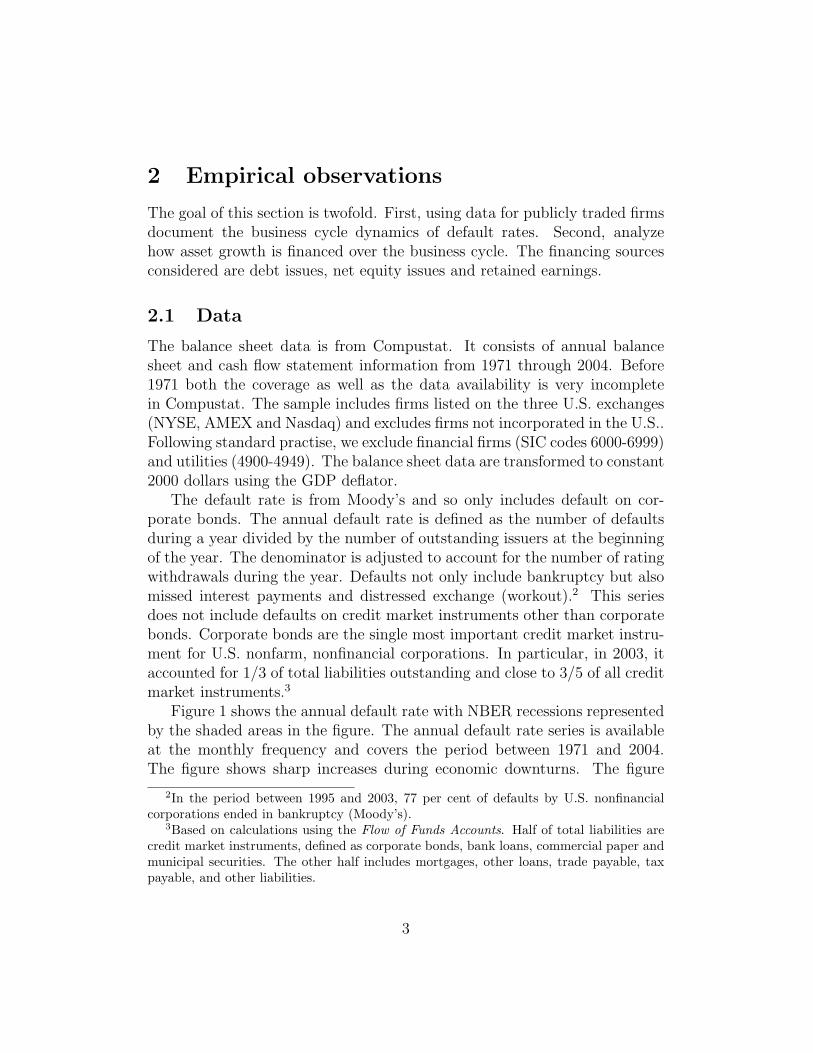
The default rate is from Moody’s and so only includes default on cor-porate bonds. The annual default rate is defined as the number of defaultsduring a year divided by the number of outstanding issuers at the beginningof the year. The denominator is adjusted to account for the number of ratingwithdrawals during the year. Defaults not only include bankruptcy but alsomissed interest payments and distressed exchange (workout).2 This seriesdoes not include defaults on credit market instruments other than corporatebonds. Corporate bonds are the single most important credit market instru-ment for U.S. nonfarm, nonfinancial corporations. In particular, in 2003, itaccounted for 1/3 of total liabilities outstanding and close to 3/5 of all creditmarket instruments.3

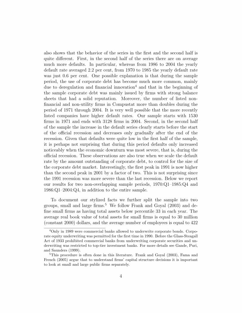
Figure 1 shows the annual default rate with NBER recessions representedby the shaded areas in the figure. The annual default rate series is availableat the monthly frequency and covers the period between 1971 and 2004.The figure shows sharp increases during economic downturns. The figure

2In the period between 1995 and 2003, 77 per cent of defaults by U.S. nonfinancialcorporations ended in bankruptcy (Moody’s).

3Based on calculations using the Flow of Funds Accounts. Half of total liabilities arecredit market instruments, defined as corporate bonds, bank loans, commercial paper andmunicipal securities. The other half includes mortgages, other loans, trade payable, taxpayable, and other liabilities.

3

also shows that the behavior of the series in the first and the second half isquite different. First, in the second half of the series there are on averagemuch more defaults. In particular, whereas from 1986 to 2004 the yearlydefault rate averaged 2.2 per cent, from 1970 to 1985 the yearly default ratewas just 0.6 per cent. One possible explanation is that during the sampleperiod, the use of corporate debt has become much more common, mainlydue to deregulation and financial innovation4 and that in the beginning ofthe sample corporate debt was mainly issued by firms with strong balancesheets that had a solid reputation. Moreover, the number of listed non-financial and non-utility firms in Compustat more than doubles during theperiod of 1971 through 2004. It is very well possible that the more recentlylisted companies have higher default rates. Our sample starts with 1530firms in 1971 and ends with 3128 firms in 2004. Second, in the second halfof the sample the increase in the default series clearly starts before the startof the official recession and decreases only gradually after the end of therecession. Given that defaults were quite low in the first half of the sample,it is perhaps not surprising that during this period defaults only increasednoticeably when the economic downturn was most severe, that is, during theofficial recession. These observations are also true when we scale the defaultrate by the amount outstanding of corporate debt, to control for the size ofthe corporate debt market. Interestingly, the first peak in 1991 is now higherthan the second peak in 2001 by a factor of two. This is not surprising sincethe 1991 recession was more severe than the last recession. Below we reportour results for two non-overlapping sample periods, 1970:Q1–1985:Q4 and1986:Q1–2004:Q4, in addition to the entire sample.

To document our stylized facts we further split the sample into twogroups, small and large firms.5 We follow Frank and Goyal (2003) and de-fine small firms as having total assets below percentile 33 in each year. Theaverage real book value of total assets for small firms is equal to 30 million(constant 2000) dollars, and the average number of employees is equal to 422

4Only in 1989 were commercial banks allowed to underwrite corporate bonds. Corpo-rate equity underwriting was permitted for the first time in 1990. Before the Glass-SteagallAct of 1933 prohibited commercial banks from underwriting corporate securities and un-derwriting was restricted to top-tier investment banks. For more details see Gande, Puri,and Saunders (1999).

5This procedure is often done in this literature. Frank and Goyal (2003), Fama andFrench (2005) argue that to understand firms’ capital structure decisions it is importantto look at small and large public firms separately.

4

Figure 1: Default Rate on Corporate Bonds

.00

.01

.02

.03

.04

.05

.06

1975 1980 1985 1990 1995 2000

Notes: The default rate series is from Moody’s (mnemonic USMDDAIWin Datastream) and it is for all corporate bonds in the US. The plotshows the annual default rate, i.e., the number of defaults during a yeardivided by the number of outstanding issuers at the beginning of theyear, adjusted by the number of rating withdrawals during the year.

5

workers. Large firms are defined as having total assets above percentile 67in each year. The average size of a large firm corresponds to 4173 million(2000) dollars. In our sample large firms employ, on average, 2200 workers.The group of small firms has an average of 703 observations per year. Thegroup of large firms is slightly bigger with an average of 940 observations peryear.

For this sample the variables of interest are aggregate net debt issues,aggregate retained earnings and aggregate net equity issues as well as theaggregate increase in assets.6 We construct the variables as in Fama andFrench (2005). Hence, net debt issues, ∆L, correspond to the change in li-abilities (Compustat data item 181) between years t and t − 1. Retainedearnings, ∆RE, is the difference between Compustat’s adjusted value of bal-ance sheet retained earnings (36) between years t and t − 1. The (book)measure of net equity issues, ∆SB, is the financing deficit minus the changein liabilities. The financing deficit is the difference between the change intotal assets and retained earnings. The change in assets, ∆A, is then givenby

∆A = ∆L + ∆RE + ∆SB. (1)

Fama and French (2005) argue that ∆SB is a noisy measure of stock is-suance.7 An alternative is the market measure of net equity issues, ∆SM ,which is the change in the number of shares between years t and t − 1 mul-tiplied by the average stock price. The change in firm’s net worth, ∆N , isequal to retained earnings plus book net equity issues. All the variables ofinterest are divided by total assets.

2.2 Stylized facts

Table 1 shows the cross-correlations between GDP and default rates for twosub-periods, 1971:Q1–1985:Q4 and 1986:Q1–2003:Q4 after both series havebeen detrended using the HP filter. The contemporaneous correlation be-tween the cyclical components of these two variables is 0.74 in the secondsub-period. It is negative but not significant in the first sub-period. For the

6The aggregate series are size-weighted averages of the firm’s individual series.7Book net equity issues are a noisy measure of stock issues for three reasons: pooling

of interest mergers, employee stock options and stock dividends. See Fama and French(2005) for details.

6

Table 1: Cross Correlations Between Default Rate and Real GDP

corr(yt+i, Φω̄t) -3 -2 -1 0 1 2 31971:Q1–2004:Q4 -0.25 -0.34 -0.38 -0.33 -0.26 -0.16 -0.08

s.e. (0.14) (0.14) (0.13) (0.13) (0.14) (0.15) (0.15)

1971:Q1–1985:Q4 -0.20 -0.22 -0.21 -0.11 -0.02 0.07 0.10s.e. (0.17) (0.16) (0.16) (0.16) (0.17) (0.17) (0.17)

1986:Q1–2004:Q4 -0.46 -0.66 -0.77 -0.74 -0.63 -0.46 -0.27s.e. (0.15) (0.11) (0.08) (0.08) (0.11) (0.15) (0.18)

Notes: The default rate series is from Moody’s (mnemonic USMDDAIW inDatastream) and it is for all corporate bonds in the US. The default rate seriesis HP filtered. Real GDP is logged and HP filtered. Standard errors are inparenthesis.

reasons highlighted above we take the second sub-period as a better proxyfor the default rates of all types of debt issues. From this evidence we drawthe first main conclusion:

Stylized fact #1: Default rates are countercyclical.

We will now turn to the balance sheet data. As pointed out by Fama andFrench (2005) and Frank and Goyal (2005) it is rare in this data set that afirm’s net equity issuance is equal to (or close to) zero. Although seasonedofferings are rare there are many ways through which firms can issue equity(warrants, convertible debt, options, etc.). This leads to the second stylizedfact:

Stylized fact #2: Non-zero equity issuance is a frequent event at the firmlevel.

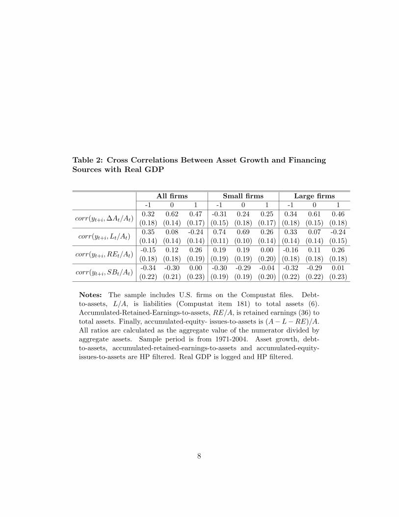
We now discuss the business cycle fluctuations of asset growth and debt-to-assets. Table 2 shows the cross-correlations between asset growth, debt-to-assets, accumulated-retained-earnings-to-assets, and accumulated-equity-issues-to-assets with real GDP after the series have been detrended using theHP filter. The contemporaneous correlation between the cyclical components

7

Table 2: Cross Correlations Between Asset Growth and FinancingSources with Real GDP

All firms Small firms Large firms-1 0 1 -1 0 1 -1 0 1

0.32 0.62 0.47 -0.31 0.24 0.25 0.34 0.61 0.46corr(yt+i,∆At/At) (0.18) (0.14) (0.17) (0.15) (0.18) (0.17) (0.18) (0.15) (0.18)

0.35 0.08 -0.24 0.74 0.69 0.26 0.33 0.07 -0.24corr(yt+i, Lt/At) (0.14) (0.14) (0.14) (0.11) (0.10) (0.14) (0.14) (0.14) (0.15)

-0.15 0.12 0.26 0.19 0.19 0.00 -0.16 0.11 0.26corr(yt+i, REt/At) (0.18) (0.18) (0.19) (0.19) (0.19) (0.20) (0.18) (0.18) (0.18)

-0.34 -0.30 0.00 -0.30 -0.29 -0.04 -0.32 -0.29 0.01corr(yt+i, SBt/At) (0.22) (0.21) (0.23) (0.19) (0.19) (0.20) (0.22) (0.22) (0.23)

Notes: The sample includes U.S. firms on the Compustat files. Debt-to-assets, L/A, is liabilities (Compustat item 181) to total assets (6).Accumulated-Retained-Earnings-to-assets, RE/A, is retained earnings (36) tototal assets. Finally, accumulated-equity- issues-to-assets is (A−L−RE)/A.All ratios are calculated as the aggregate value of the numerator divided byaggregate assets. Sample period is from 1971-2004. Asset growth, debt-to-assets, accumulated-retained-earnings-to-assets and accumulated-equity-issues-to-assets are HP filtered. Real GDP is logged and HP filtered.

8

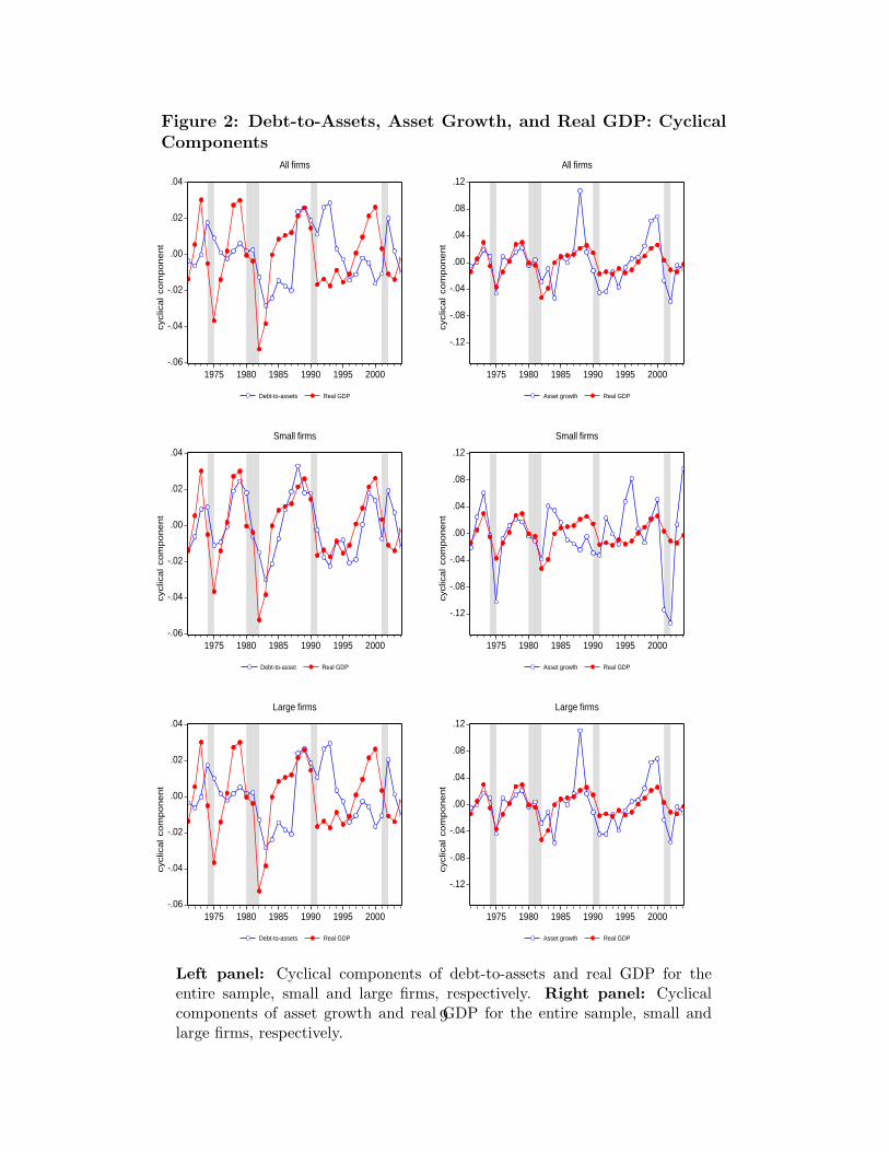
Figure 2: Debt-to-Assets, Asset Growth, and Real GDP: CyclicalComponents

-.06

-.04

-.02

.00

.02

.04

1975 1980 1985 1990 1995 2000

Debt-to-assets Real GDP

cycl

ica

l co

mp

on

en

tAll firms

-.12

-.08

-.04

.00

.04

.08

.12

1975 1980 1985 1990 1995 2000

Asset growth Real GDP

cycl

ica

l co

mp

on

en

t

All firms

-.06

-.04

-.02

.00

.02

.04

1975 1980 1985 1990 1995 2000

Debt-to-asset Real GDP

cycl

ica

l co

mp

on

en

t

Small firms

-.12

-.08

-.04

.00

.04

.08

.12

1975 1980 1985 1990 1995 2000

Asset growth Real GDP

cycl

ica

l co

mp

on

en

tSmall firms

-.06

-.04

-.02

.00

.02

.04

1975 1980 1985 1990 1995 2000

Debt-to-assets Real GDP

cycl

ica

l co

mp

on

en

t

Large firms

-.12

-.08

-.04

.00

.04

.08

.12

1975 1980 1985 1990 1995 2000

Asset growth Real GDP

cycl

ica

l co

mp

on

en

t

Large firms

Left panel: Cyclical components of debt-to-assets and real GDP for theentire sample, small and large firms, respectively. Right panel: Cyclicalcomponents of asset growth and real GDP for the entire sample, small andlarge firms, respectively.

9

of asset growth with real GDP is 0.6. Interestingly, the comovement for smallfirms is 0.24 and not statistically different from zero. This is not surprisingif one takes into consideration that small firms are more likely to be growingeven when the economy is not booming. On the other hand asset growthfor large firms is strongly procyclical with a contemporaneous correlation of0.60 with output. In addition, the correlation between debt-to-assets and realGDP is positive, but not statistically different from zero. Only for small firmsis debt-to-assets strongly procyclical and moreover it lags output. For largefirms debt-to-assets is acyclical. All these observations are consistent withthe idea small firms face financing constraints. Otherwise we would expectto observe asset growth to be procyclical as we observe for large firms. Inaddition, we would also expect debt-to-assets to be acyclical, assuming nochanges in taxes.

For the other financing sources the cross correlations are not statisticallydifferent from zero. Accumulated-retained-earnings-to assets is positivelycorrelated with output and accumulated-equity-issues-to-assets is negativelycorrelated with output, but the comovements are not striking. Figure 2displays the cyclical components of debt-to-assets, asset growth and realGDP. These plots show sharp decreases during economic downturns, speciallyfor small firms. We summarize these observations as follows:

Stylized fact #3: Asset growth is procyclical for large firms. It is onlyslightly cyclical for small firms. Debt-to-assets is only procyclical for smallfirms and lags output.

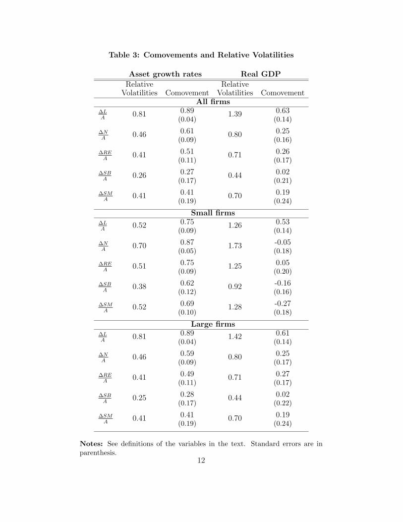
We now consider the cyclical behavior of the three sources of financing:debt issues, ∆L/A, retained earnings, ∆RE/A, and equity issues, ∆SB/A.We also look at the change in net worth, ∆N = ∆RE + ∆SB. To illustratethe importance of firm size we again separate firms into two other groups—small and large firms— in addition to the total sample. Table 3 summarizesthe contemporaneous correlation between the three sources of financing withasset growth and GDP . In particular, the comovement between asset growthand net debt issues is 0.9 for large firms and 0.7 for small firms. The tablealso plots the standard deviation of the change in each (scaled) finance sourcerelative to the standard deviation of asset growth. Here we find a strikingdifference between small firms and large firms. The relative volatility ofboth retained earnings and equity issuance is higher for small firms thanfor large firms, whereas the opposite is true for debt finance. In particular,the standard deviation of ∆N/A is 70 per cent of the standard deviation of

10

∆A/A for small firms, whereas for large firms this number is only 46 percent.

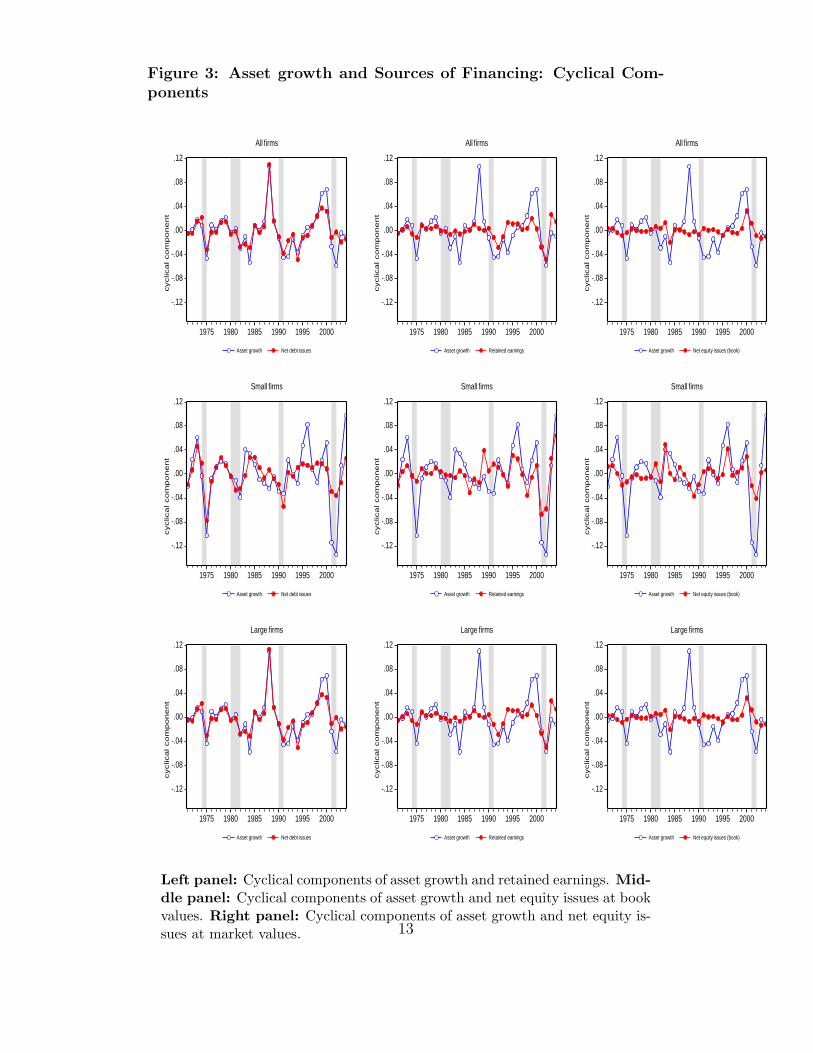
The panels in Figure 3 plot asset growth for the corresponding firm cate-gory together with a financing source. The graphs illustrate the correlationsresults of Table 3. In particular, the left panels shows that net debt issuescomove very closely with asset growth for all firm categories, but especiallyfor large firms. Also, the importance for small firms of both retained earningsand net equity issuance is clearly visible.

The middle and right panel of Figure 3 displays the cyclical behaviorof retained earnings and net equity issues with asset growth. A graphicalinspection of these plots confirms the result that the comovement betweenretained earnings and asset growth is more evident for small firms. We alsoobserve a similar pattern between equity issues and asset growth.

Figure 3 shows a dramatic increase in asset growth and net debt issuesfor large firms that occurred in 1988. First, this was a year of unusualcorporate restructuring activity, in particular in the form of leverage buyoutsand stock repurchases. Second, a new accounting rule was introduced thatrequired companies to consolidate the balance sheets of their wholly ownedsubsidiaries (Bernanke, Campbell, and Whited, 1990). This observation hasa small effect on our results. For example, eliminating this observation fromour sample changes the contemporaneous correlation between asset growthand net debt issues, retained earnings, and net equity issuance for large firmsto 0.85, 0.59 and 0.40, respectively. These results lead us to the followingobservation:

Stylized fact #4: At the aggregate level we find that asset growth in largefirms is mostly debt financed. Asset growth in small firms is driven by allthree sources of financing, debt, retained earnings and equity issues.

3 External finance in the literature

The idea that agency problems cause a wedge between the expected ratethat firms pay on outside financing and the opportunity cost of using re-tained earnings has been well established in the literature.8 In the corporatefinance literature there are now several papers that consider models in whichthere is a choice between debt and external equity (and both are subject to an

8Probably reference the Stiglitz handbook chapter for an early survey.

11

Table 3: Comovements and Relative Volatilities

Asset growth rates Real GDP

Relative RelativeVolatilities Comovement Volatilities Comovement

All firms0.89 0.63∆L

A0.81

(0.04)1.39

(0.14)

0.61 0.25∆NA

0.46(0.09)

0.80(0.16)

0.51 0.26∆REA

0.41(0.11)

0.71(0.17)

0.27 0.02∆SBA

0.26(0.17)

0.44(0.21)

0.41 0.19∆SMA

0.41(0.19)

0.70(0.24)

Small firms0.75 0.53∆L

A0.52

(0.09)1.26

(0.14)

0.87 -0.05∆NA

0.70(0.05)

1.73(0.18)

0.75 0.05∆REA

0.51(0.09)

1.25(0.20)

0.62 -0.16∆SBA

0.38(0.12)

0.92(0.16)

0.69 -0.27∆SMA

0.52(0.10)

1.28(0.18)

Large firms0.89 0.61∆L

A0.81

(0.04)1.42

(0.14)

0.59 0.25∆NA

0.46(0.09)

0.80(0.17)

0.49 0.27∆REA

0.41(0.11)

0.71(0.17)

0.28 0.02∆SBA

0.25(0.17)

0.44(0.22)

0.41 0.19∆SMA

0.41(0.19)

0.70(0.24)

Notes: See definitions of the variables in the text. Standard errors are inparenthesis.

12

Figure 3: Asset growth and Sources of Financing: Cyclical Com-ponents

-.12

-.08

-.04

.00

.04

.08

.12

1975 1980 1985 1990 1995 2000

Asset growth Net debt issues

cyclica

l co

mp

on

en

t

All firms

-.12

-.08

-.04

.00

.04

.08

.12

1975 1980 1985 1990 1995 2000

Asset growth Retained earnings

cyclica

l co

mp

on

en

t

All firms

-.12

-.08

-.04

.00

.04

.08

.12

1975 1980 1985 1990 1995 2000

Asset growth Net equity issues (book)

cyclica

l co

mp

on

en

t

All firms

-.12

-.08

-.04

.00

.04

.08

.12

1975 1980 1985 1990 1995 2000

Asset growth Net debt issues

cyclica

l co

mp

on

en

t

Small firms

-.12

-.08

-.04

.00

.04

.08

.12

1975 1980 1985 1990 1995 2000

Asset growth Retained earnings

cyclica

l co

mp

on

en

t

Small firms

-.12

-.08

-.04

.00

.04

.08

.12

1975 1980 1985 1990 1995 2000

Asset growth Net equity issues (book)cyclica

l co

mp

on

en

t

Small firms

-.12

-.08

-.04

.00

.04

.08

.12

1975 1980 1985 1990 1995 2000

Asset growth Net debt issues

cyclica

l co

mp

on

en

t

Large firms

-.12

-.08

-.04

.00

.04

.08

.12

1975 1980 1985 1990 1995 2000

Asset growth Retained earnings

cyclica

l co

mp

on

en

t

Large firms

-.12

-.08

-.04

.00

.04

.08

.12

1975 1980 1985 1990 1995 2000

Asset growth Net equity issues (book)

cyclica

l co

mp

on

en

t

Large firms

Left panel: Cyclical components of asset growth and retained earnings. Mid-dle panel: Cyclical components of asset growth and net equity issues at bookvalues. Right panel: Cyclical components of asset growth and net equity is-sues at market values. 13

external finance premium).9 Since GDP is produced mainly in firms that canissue equity10 it is important to allow for external equity in macro models ofthe business cycle. Almost all DSGE models that incorporate agency prob-lems in firm finance, however, restrict external finance to debt contracts. Thefirst subsection discusses the alternative approaces used. Next, we discusswhich agency problem is the basis of our framework and which modificationswe introduce to improve key predictions of the model.

Take the money and run One possible problem that a lender may beconcerned about is that the borrower takes the funds and either squandersthe money or moves to a place on earth where he cannot be harassed by thelender. This is the agency problem considered in Kiyotaki and Moore (1997)(KM henceforth). In particular, KM assume that a borrower will alwaysrun away with any funds it could run away with. Consequently, lenders willrequire collateral and in particular the amount they lend has to be less thanthe value of the collateral. KM assume that there are two types of producers,farmers and gatherers, and both use the fixed factor (land), which is not onlyproductive but can also serve as collateral. KM choose parameters such thatthe farmers borrow from the gatherers, are constrained in the amount theycan borrow, and at the margin are more productive. Let rl be the lendingrate, k the amount of the fixed factor in the hands of the constrained agents,and q′ the value of the collateral in the next period. Then the amount offunds borrowed, b has to satisfy the following equation.

(1 + rl)b ≤ q′k. (2)

KM show that this framework generates two appealing predictions.First, an increase in productivity leads to an increase in profits and,

thus, an increase in net worth for constrained firms, which in turn makes itpossible for the firm to borrow more. This leads to an increase in the scaleof production by constrained firms and a further increase in the net worthin the next period. Consequently, a one-time increase in productivity canlead to a persistent increase in the demand of the fixed factor through theso-called net-worth channel. In general equilibrium, an increase in the useof the fixed factor by constrained agents must lead to a reduction in the use

9See for example Moyen (2004) and Hennessy and Whited (2005).10According to the Economic Report of the President, 2003, corporations account for

approximately 60 per cent of GDP.

14

by unconstrained agents. But because constrained agents are assumed to bemore productive, this reallocation of resources does lead to an increase inaggregate productivity. To understand the effect of net worth on the amountthe firm can borrow, consider the budget constraint of the borrower, whichis given by

qk = n + b, (3)

where n is the net worth of the agent. Suppose that the borrowing constraintis binding. Then it is easy to show that(

1 + rl

q′/q− 1

)b = n. (4)

The term in brackets is the real rate of return, that is, the nominal rate ofreturn adjusted for the increase in value of the collateral. The amount afirm can borrow is, thus, determined by the condition that the amount of networth has to be equal to the real interest payments. This condition impliesquite a high leverage ratio. KM also consider a modification of the modelin which cultivating the fixed factor requires additional (uncollaterizable)investment. This reduces the leverage factor.

The second appealing prediction of the KM framework is that the value ofcollateral increases in response to a positive shock. An important componentof net worth, n, is the value of the existing fixed factor, qk−1. Consequently,an increase in the demand for this factor leads to an increase in the valueof the firm’s net worth and, thus, through the channel described above to afurther increase in the demand of the fixed factor. Note that the value ofcollateral is not only pushed up by the current increase in the demand for thefixed factor, but—since it is a durable asset—also by the increased demand insubsequent periods. The framework, therefore, delivers an appealing within-period and intertemporal multiplier process.

It is hard to believe, however, that a big concern for lenders in developedeconomies is that managers divert firm resources in a way that none is leftfor the lender. Indeed, a substantial fraction of business loans does not havecollateral.11 Moreover, the existence of collateralized loans doesn’t meanthat this agency problem is important. A collateralized loan is basicallya loan that gives the lender priority when bankruptcy occurs and this is

11xxx

15

advantageous even if bankruptcy occurs for other reasons than diversion ofassets.

Furthermore, KM rely on linear production functions and an infinite elas-ticity of intertemporal substitution. Cordoba and Ripoll (2004) show that ifone relaxes those assumptions the effects are quantitatively important onlyfor empirically implausible values. Moreover, if parameters are such thatshocks lead to a substantial increase in leverage (and investment) then thecorresponding increase in interest rates will be strong as well. This will sub-stantially dampen the effect on net worth in the next period and thus reducepersistence.12

Limited contract enforceability The contracting environment in KMis very simple. Lending is assumed to occur through one-period lendingcontracts. Moreover, defaults never occur since loans are fully collateral-ized. An alternative approach followed in the literature is to design optimalcontracts in which the lender commits to a sequence of state contingents cap-ital allocations to the firm and payments to the entrepreneur. Albuquerqueand Hopenhayn (2004) and Cooley, Marimon, and Quadrini (2004) use thisapproach and derive the optimal contract in an environment in which theborrower can divert the assets of the firm as in KM.

An attractive feature of these papers is that they can explain firm growth.In particular, the amount of capital assets under the control of the firmremains constant until the enforcement constraint is binding, that is, whenthe entrepreneur is tempted to divert the funds. If that happens then theamount of capital is increased and the temptation to divert funds is preventedby making the current relationship more attractive. In Cooley, Marimon, andQuadrini (2004) a positive aggregate shock represents a higher probabilitythat a new project will have high productivity. The aggregate shock doesn’taffect the productivity of existing projects. Consequently, entrepreneurs aremore tempted to divert the capital of the existing relationship and start anew project. This means that for more firms the enforcement constraint willbe binding and the amount of funds received from the lender will increase.The optimal contract, thus, has the attractive property that a productivityshock is magnified by the increased allocation of funds to firms.

12Kocherlakota (2000) makes a similar point but he doesn’t allow for a reallocation ofthe fixed factor from productive to unproductive agents. As shown in the appendix, withno variation in use of the fixed factor the leverage effect of KM is eliminated.

16

Less appealing is that these additional funds are given because it is ex-actly during good times that entrepreneurs are more likely to divert capitaland entrepreneurs will remain loyal to the existing contract only if it is mademore attractive. Another undesirable feature is that firms—as in KM—neverdefault. Also, Quadrini (2004) points out that state-contingent optimal con-tracts may not be renegotiation proof. That is, it may be possible that boththe lender and the entrepreneur would prefer to renegotiate the contract.Quadrini (2004) designs the optimal contract that adds as an additionalrestriction that it is renegotiation proof. Interestingly, he shows that (ran-domized) liquidation may be part of that renegotiation proof contract in anenvironment in which liquidation would not be part of the optimal contract.13

Other moral hazard problems The assumption that the entrepreneurcan divert the assets of the firm creates a particular (and quite extreme)moral hazard problem. Besides diverting the assets and leaving nothingto the creditor, there are other—less extreme—entrepreneurial actions thatdiminish the chance for the lender to get his money back. For example, therevenues could depend on the effort put in by the entrepreneur. Also, theamount of risk chosen by the manager may be hard to control by the lender.One would think that these are more plausible concerns than diverting assets.Although this agency problem has received considerable attention in theliterature, there are few papers that have incorporated an unverifiable effortor investment choice into DSGE models. One exception is the paper by denHaan, Ramey, and Watson (2003) in which the outcome of the project isaffected by the effort choice of the entrepreneur. The model in den Haan,Ramey, and Watson (2003) has besides this moral hazard problem also amatching friction, so that it takes time for a borrower to find a lender, andan inefficient allocation of funds across lenders. The latter friction impliesthat lenders who are in a relationship with a borrower may not have enoughfunds to write a sustainable contract, which stands in sharp contrast with therest of the literature that assumes that lenders have unlimited access to funds.Unlimited access to funds may not always be an appropriate assumption. Forexample, bank equity regulation makes the ability of banks to extend loansdependent on the amount of bank equity, which is not easy to adjust.

13Quadrini (2004) also considers an environment in which the scrap value of the firmmay exceed the joint value of the contract. In that environment liquidation can be partof the optimal contract as well.

17

Another example of a model that incorporates a more realistic moralhazard problem is the DSGE model in Covas (2004) who considers a modelin which the manager of the firm chooses the risk of the project undertaken.An important feature of Covas (2004) is that the objectives of the owner andthe manager do not necessarily coincide. This stands in sharp contrast withthe rest of the papers in the macro literature in which the owner and themanager are typically the same agent.

Asymmetric information Uncertainty is an important source of agencyproblems. One possibility is that there is asymmetric information about thecharacteristics of the borrower when the contract is written. We are notaware of DSGE models that incorporate this type of agency problem. Giventhat the probability of drawing a ”lemon” may very well increase during adownturn this may be an interesting approach. Another important reasonwhy uncertainty matters is that the outcome of a project is random (even ifthe borrower puts in the best possible effort). The question arises whetherthis in itself leads to an increase in the external financing premium. In aclassic paper, Townsend (1979) shows that if it is costly for the lender toobserve the realization of the shock, then the optimal contract to deal withthis agency problem is a debt contract. The relevant cost in the costly-state-verification (or CSV) framework is the cost the lender has to incur todetermine the outcome of the realization. In the literature, observed bank-ruptcy costs are often used to calibrate the magnitude of these verificationcosts. But this is a bit odd, since the actual verification costs are likely tobe much smaller than typical bankruptcy costs. Moreover, we are not awareof any evidence that suggests that the verification itself is very costly.

One-period debt contracts and uncertain outcomes Note, however,that the assumption that it is costly to determine how much resources areleft in the firm is only needed for the result that the one-period contract isthe optimal contract. If there are other reasons why state-contingent lendingcontracts are not feasible and lending occurs through one-period debt con-tracts (for example because of habits, convenience, or simplicity) then onecan not only use this framework but one can also calibrate the model usingobserved bankruptcy costs. All equations, including those that determinewhat contract among all one-period debt contracts is the optimal one, areexactly the same as in the CSV framework. The only difference is that if

18

verification costs are negligible then the model by itself does not imply thatthe one-period debt contract is the optimal contract.

Properties of the CSV framework An attractive feature of the opti-mally chosen one-period debt contract is that the amount lent increases withthe net worth of the agent as well as the expected productivity of the firm.Consequently, as shown, for example, in Carlstrom and Fuerst (1997), thisframework is helpful in propagating shocks through the so called net-worthchannel. A positive shock increases net worth which increases the scale ofoperations, profits, and, thus, next period’s net worth. This in turn leads toan increase in lending. A not so attractive feature is that defaults increasewith aggregate productivity. That is, an increase in aggregate productivityleads to such an increase in the scale of the project that default happensmore frequently. Moreover, the assumption of linear production technologyimplies that the subsequent increase in net worth has no effect on defaultrates. Bernanke, Gertler, and Gilchrist (1999) assume that the realization ofthe aggregate productivity is not yet know when the debt contract is deter-mined. This means that an unexpectedly high aggregate productivity shocksresults in a lower default rate. But they still have the property that anincrease in the expected productivity leads to an expected increase in thedefault rate.14

We discuss the reasons for the procyclical default rate in this frame-work in more detail in Section 5.1. We also propose two modifications. Thefirst modification is to replace the linear technology production function bya standard production function that satisfies decreasing marginal returns.With this production function, we find that increases in net worth have anegative effect on the default rate. The second modification adds an ad-ditional component to the production function. With this specification, itis easy to find parameters such that an increase in aggregate productivityreduces the default rate.

Bernanke, Gertler, and Gilchrist (1999) add adjustment costs of capital toreinforce the net-worth channel. With adjustment costs an increased desireto invest leads to an increase in the price of the capital. This means that apositive productivity shock increases the value of net-worth not only becauseof the increase in retained earnings but also because of the increase in the

14I think this is true but needs to be checked.

19

market value of the capital stock.15 We find such a valuation effect veryplausible and an attractive feature of the model to have. However, an increasein the price of capital because of the difficulty to quickly produce additionalcapital is likely to be only a part of the increased value of the firm duringgood times. Moreover, if productivity increases are not embodied in existingcapital then the price of existing capital might even go down. In Cooley andQuadrini (2001) net worth of the firm represents the earnings potential ofthe firm. This is the approach we follow in this paper.

Predictions of the different frameworks The agency problems dis-cussed above are quite different. Nevertheless,changes in net worth andproductivity have similar effects on real activity, that is, these models allpredict that an increase in productivity leads to an increase in real activity,which over time leads to an increase in net worth and a reduction in the ex-ternal finance premium. There are important differences in the predictions ofthese different approaches as well. As discussed above, in some frameworksdefault doesn’t occur and in some frameworks, the default rates are even pro-cyclical. The frameworks also differ in the importance of changes in the riskfree or discount rate. If a firm is nothing more than a stock of capital stockand produced commodities can be transformed into investment commodities(either one for one or at a slightly higher rate in the presence of adjustmentcosts), then there is no direct effect of the discount rate. However, if part ofthe firm are assets that are in fixed supply then the value of the firm is thediscounted value of the earnings generated by this fixed asset and changesin the discount rate are then likely to have strong effects on the value of thefirm.

Even across papers that use the same framework we find important differ-ences in the choices needed to implement the problem. For example, in ? thesavings decision of the entrepreneur has an interior solution.16 This meansthat entrepreneurs withdraw funds from the firm every period. Depend-ing on how the entrepreneur changes his consumption level in response to a

15Note that with the linear production function typically assumed in this literature, thismodification doesn’t affect the result that changes in net worth have no impact on thedefault rate.

16That is, the savings decision affects the price of the commodity produced by the sectorwith the agency problem. In equilibrium, this price will adjust every period so that theEuler equation of the savings decision has an interior solution.

20

shock this can either dampen or reinforce the net worth channel.17 Bernanke,Gertler, and Gilchrist (1999) on the other hand choose parameters such thatentrepreneurs choose to keep all funds within the firm. Bernanke, Gertler,and Gilchrist (1999) prevent the net worth of firms to go to infinity by as-suming that firms exogenously stop operating with some probability in whichcase the owners consume the net worth of the firm.

Making magnification possible in general equilibrium So far, theprofession has not been successful in identifying external shocks that arelarge enough to explain the observed fluctuations in economic aggregates.18

Therefore, the recent literature has tried to build DSGE models in whichshocks are magnified and propagated and models with agency problems havebeen the main contender.19

It is important to realize though that in a general equilibrium this isnot enough to magnify and/or propagate shocks. If firms increase the scaleof their operation the question arises where the additional resources comefrom. One possibility is that entrepreneurs decrease their consumption andinvest the additional funds in the firm.20 In numerous papers, however,the high return on retained earnings forces the consumption level of theentrepreneur to be at a corner so that no further reductions in consumptionare possible. Moreover, even if the entrepreneur increases the amount ofretained earnings, this still wouldn’t answer the question where the additionalfunds provided by the lender come from. Some papers simply assume thatlenders have unlimited access to funds at an interest rate that is not affectedby the shock.21 This may be a plausible assumption when one studies theeffect of a country-specific shock for a small country with excellent accessto international funds. In this case the resources to finance the expansioncome from abroad. Interest rates would also be constant if savers have a

17For example, in ? a positive productivity shock does indeed lead to a sharp reductionin the amount of entrepreneurial consumption but is then followed by a moderate increasebut this result may change if nonlinear utility functions for the entrepreneur are considered.

18See Cochrane (1994), for example.19Alternatives are models with sun spots such as XXX or models with labor market

frictions such as Andolfatto (XXX), Merz (XXX), and Den Haan, Ramey, and Watson(2000).

20But note that if the risk smoothing motive is strong enough, then entrepreneurs wouldlike to increase their consumption.

21Papers that make this assumption are Kocherlakota (2000), Cooley, Marimon, andQuadrini (2004), xxx.

21

very high intertemporal elasticity of substitution. In this case the expansionwould be financed by a reduction in (the growth of) aggregate consumption.Of course, this does lead to the counterfactual implication that consumptionis countercyclical.

In this respect, the analysis of KM is quite interesting. Although KMassume that interest rates are constant, the key factor of production in theiranalysis is in fixed supply. Consequently, the expansion is financed by areallocation of the factor from less productive to more productive agents.Unfortunately, Cordoba and Ripoll (2004) show that if one relaxes the as-sumptions of constant interest rates and constant marginal productivity thatit is difficult to generate quantitatively interesting results in the KM frame-work. Although, Cordoba and Ripoll (2004) focus on the agency problem ofKM, the message of their paper is likely to carry over to other environments.For example, if the borrowing constraints are relaxed and intermediaries aremore willing to lend out funds, then the risk free rate may have to increaseto attract these additional funds from depositors.

Note that in a framework such as CSV that has a procyclical default ratethis problem is even worse since it means that more resources are lost dueto the increased bankruptcy rate. In fact, in Carlstrom and Fuerst (1997,1998) this effect is so strong that even in later periods, when the increase inentrepreneurial net worth has reduced agency problems, the output responseis only marginally above the output response of the standard real businesscycle model.

Consequently, agency costs by themselves may not be enough to generatea framework with quantitatively interesting magnification and propagationeffects. In addition, one would need a mechanism through which aggregateresources increase. One mechanism is the increase in labor supply. Empiri-cal estimates of the labor supply elasticities make clear that changes in theintensive margin are likely to be weak but changes in the extensive marginare empirically more plausible. den Haan, Ramey, and Watson (2000) builda labor market matching model into a general equilibrium framework andshow that changes in the extensive margin are important in magnifying andpropagation shocks.

22

4 Our framework

4.1 Summary

The starting point in this paper is the CSV framework. In particular, weassume the following:

• Default leads to the loss of resources.

• The idiosyncratic shock has not yet been realized when the lendingcontract is written.

• Lending occurs through one-period loans and borrowers are protectedby limited liability. If the costs associated with default are verificationcosts then the one-period contract is the optimal type of contract. It isnot clear to us, however, that the actual verification costs are very highand these are likely to be tiny relative to bankruptcy cost. Since thereare other reasons (e.g., simplicity of habit) to motivate one-period debtcontracts, we are perfectly happy simply assuming that this is one typeof contract used by firms. Note that if one restricts the contract to bea one-period debt contract then all bankruptcy costs are relevant.

• The parameters of the one-period debt contract are chosen to maxi-mize the expected profits of the entrepreneur subject to the break-evencondition of the lender.

• We assume that consumption and investment commodities are pro-duced with the same technology and the aggregate shock considered isa change in the productivity of this technology.22

Using this framework we modify the model in the following three ways.

22In Carlstrom and Fuerst (1997) the production of investment commodities occurs infirms that suffer from agency problems, whereas the production of consumption commodi-ties is not subject to agency problems. A positive aggregate productivity shock increasesthe productivity of the technology to produce consumption commodities, but endogenouslyraises the prices at which entrepreneurs can sell the investment commodity. A consequenceof not having the the endogenous price is that we cannot use the standard Euler equationto obtain an interior solution for the (aggregate) dividend choice.

23

• We consider a technology with diminishing marginal productivity ofcapital (instead of constant) and production incurs a fixed cost. Thefirst modification generates a default rate that is decreasing with networth, whereas the default rate does not depend on net worth when thetechnology is linear. The second modification implies that the defaultrate is decreasing with aggregate productivity, whereas it is increasingwithout fixed costs.

• We consider a model in which firm entry is restricted. Consequently,the net worth of the firm is affected by the discounted value of futureearnings. This can also overturn the result that the default rate is pro-cyclical. In Cooley and Quadrini (2001), the net worth of the firm alsodepends on expected future earnings, but quantitatively this doesn’tplay a big role in their setup. In particular, increases in the discountedvalue of future earnings are not strong enough to overturn the positiverelationship between firm productivity and the default rate. More im-portantly, they do not consider aggregate uncertainty, so they cannotaddress the question how important these changes in discounted futureearnings are for the business cycle dynamics of this type of model.23

• We allow the firm to attract outside equity. The standard approach isto assume that net worth can only increase through retained earnings.An important exception is Cooley and Quadrini (2001, 2005). In thesepapers, there is a linear cost of issuing equity, which means that firmswill not pay dividends until the firm has reached a certain size. In Sec-tion 2 we pointed out that this is inconsistent with empirical evidence.We assume that the costs of issuing equity are continuous and strictlyconvex. With this approach firms issue equity much more frequently.

An important part of this paper is to modify the CSV framework so thatit generates countercyclical default rates. We do this simply by consideringan alternative production function. An alternative is proposed in Bernanke,Gertler, Gilchrist (1999). They assume that the contract is written beforeaggregate productivity is known. An increase in z means that there are more

23Cooley and Quadrini (2005) do consider aggregate shocks but in that paper agencyproblems are exogenously imposed (the amount of debt has to be less than the firm’sequity). That is, there are no defaults and the value of the firm does not affect theexternal finance premium.

24

resources in the firm than expected and the default rate decreases. We findthis solution not quite satisfying since an increase in the expected value of zstill increases the default rate.

5 Generating a countercyclical default rate in

a CSV framework

The standard implementation of the CSV framework has the counterfactualprediction that the default rate is countercyclical. There are two reasons forthis prediction. First, keeping net worth constant, an increase in aggregateproductivity leads to an increase in the default rate. Second, the increase innet worth that follows the increase in aggregate productivity has no effect onthe default probability. In the first subsection we explain these predictions.In the second section we provide two modifications, namely diminishing mar-ginal returns and the introduction of a fixed cost (or benefit), and show thatwith these modifications the framework can generate the desired responsesof the default rate to changes in net worth and aggregate productivity.

5.1 Procyclical default rates in the standard CSV frame-work

In this section we describe the standard CSV model and we discuss why networth has no effect on the default rate and why productivity has a positiveeffect.

5.1.1 Static CSV framework

Entrepreneurs have access to the following technology:

zωk, (5)

where k stands for the amount of capital, z for the aggregate productivityshock (with z > 0), and ω for the idiosyncratic productivity shock (withω ≥ 0). We assume that z is observed at the beginning of the period whenthe debt contract is written, but that ω is only observed at the end of theperiod. The entrepreneur’s net worth is equal to n and he borrows (i − n).

25

Borrowing occurs through one-period debt contracts.24 That is, the borrowerand lender agree on a debt amount, (i − n), and a lending rate, rl. Theentrepreneur defaults if the resources in the firm are not enough to pay backthe amount borrowed plus interest. That is, the entrepreneur defaults if ω isless than the default threshold, ω, where ω satisfies

zωk = (1 + rl)(i − n). (6)

If the entrepreneur defaults then the lender gets

zωk − µzωk, (7)

where µ represent bankruptcy costs, which are assumed to be a fractionof revenues.25 Note that in an economy with µ > 0 default is inefficientand would not happen if the first-best solution could be implemented. LetΦ(ω) be the cdf of the idiosyncratic productivity shock. We can then writeexpected entrepreneurial income as

∞∫ω

zωkdΦ(ω) − (1 − Φ(ω))(1 + rl)(i − n). (8)

The expected income of the lender is given by

(1 − Φ(ω))(1 + rl)(i − n) +

ω∫−∞

zωkdΦ(ω) − µzk

ω∫−∞

ωdΦ(ω). (9)

We follow standard practice and assume that the lender only cares about hisexpected income.26 This requires that the lender is either risk neutral or hasa well-diversified portfolio. Given values for n and z, the financial contractspecifies a debt amount, k − n, and a lending rate, rl, which then imply avalue for ω. Alternatively, one can use (6) and define the financial contractas the pair (k, ω). If we use (6) then we can write the entrepreneur’s expectedincome as

24If the default costs introduced below are the costs the lender pays to verify the real-ization of the idiosyncratic shock then we have the CSV framework of Townsend (1979)and the one-period debt contract is the optimal type of contract.

25In section 6 we consider alternatives.26Note that z is known when the contract is written.

26

zkF (ω) with F (ω) =

∞∫ω

ωdΦ(ω) − (1 − Φ(ω))ω (10)

and the lender’s expected revenues as

zkG(ω) with G(ω) = (1 − Φ(ω))ω + (1 − µ)

ω∫−∞

ωdΦ(ω) (11)

We assume that the entrepreneur is risk neutral. For given values of nand z the values of (k, ω) are then chosen to maximize the expected entre-preneurial income subject to the constraint that the lender must break even.For simplicity we assume in this section that the cost of funds for the lenderis equal to zero. The best one-period debt contract is, thus, given by thefollowing maximization problem:

maxk,ω

zkF (ω)

s.t. zkG(ω) = k − n

(12)

The optimal values for k and ω are given by

zF (ω)

1 − zG(ω)= −∂F (ω)/∂ω

∂G(ω)/∂ωand (13)

k =n

1 − zG(ω). (14)

Below we will build intuition using the slopes of the iso-profit and zero-profit curves. The slope of the iso-profit curve is given by

dk

dω= −k∂F (ω)/∂ω

F (ω)(15)

and the slope of the zero-profit curve is given by

dk

dω=

zk∂G(ω)/∂ω

1 − zG(ω). (16)

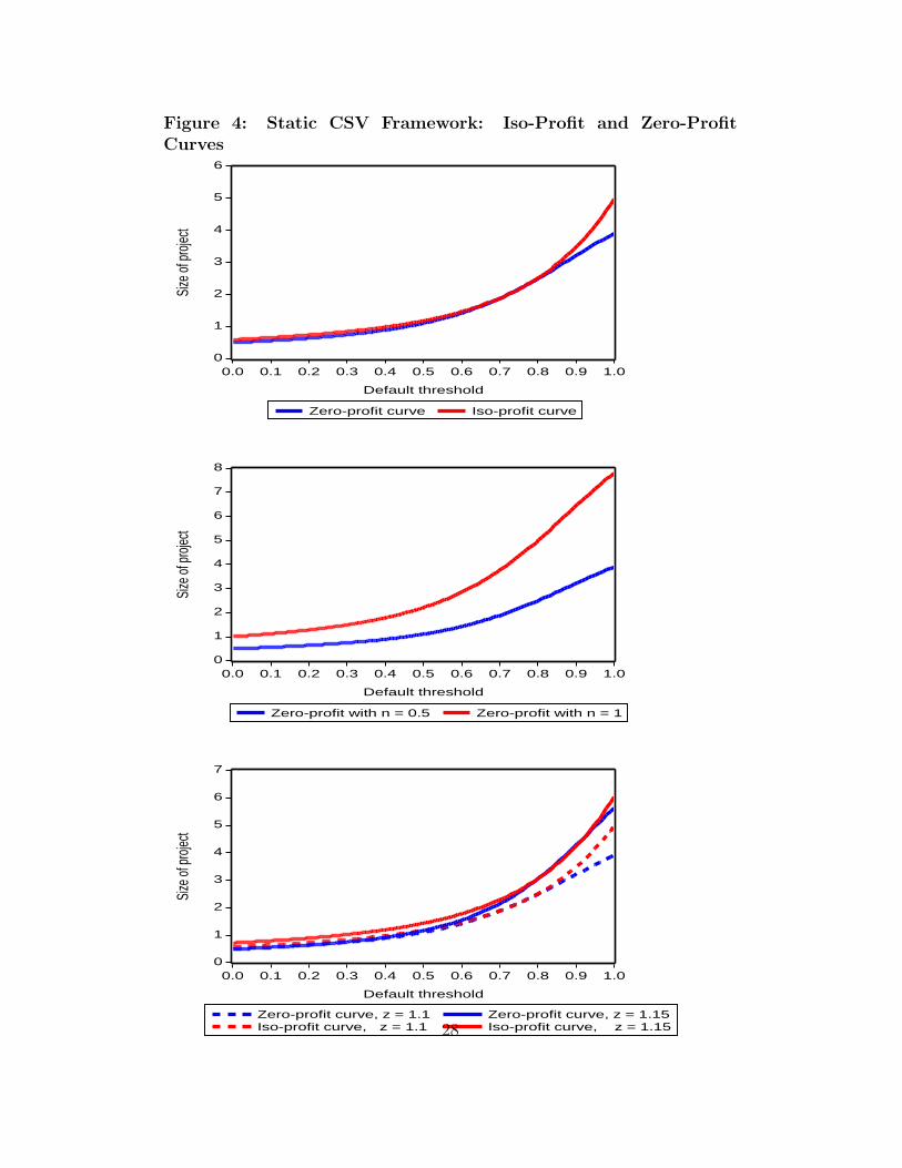
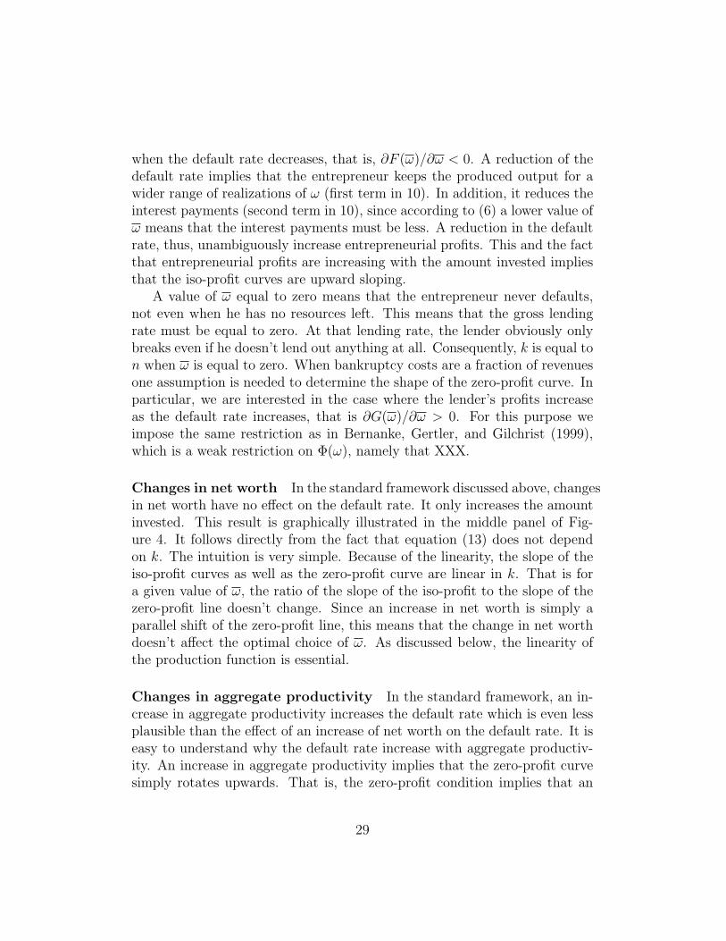
The top panel in Figure 4 shows the iso-profit curve for the entrepreneurand the zero-profit condition of the lender. Entrepreneurial profits increase

27

Figure 4: Static CSV Framework: Iso-Profit and Zero-ProfitCurves

0

1

2

3

4

5

6

0.0 0.1 0.2 0.3 0.4 0.5 0.6 0.7 0.8 0.9 1.0

Default threshold

Zero-profit curve Iso-profit curve

Size

of pr

oject

0

1

2

3

4

5

6

7

8

0.0 0.1 0.2 0.3 0.4 0.5 0.6 0.7 0.8 0.9 1.0

Default threshold

Zero-profit with n = 0.5 Zero-profit with n = 1

Size

of pr

oject

0

1

2

3

4

5

6

7

0.0 0.1 0.2 0.3 0.4 0.5 0.6 0.7 0.8 0.9 1.0

Default threshold

Zero-profit curve, z = 1.1Iso-profit curve, z = 1.1

Zero-profit curve, z = 1.15Iso-profit curve, z = 1.15

Size

of pr

oject

28

when the default rate decreases, that is, ∂F (ω)/∂ω < 0. A reduction of thedefault rate implies that the entrepreneur keeps the produced output for awider range of realizations of ω (first term in 10). In addition, it reduces theinterest payments (second term in 10), since according to (6) a lower value ofω means that the interest payments must be less. A reduction in the defaultrate, thus, unambiguously increase entrepreneurial profits. This and the factthat entrepreneurial profits are increasing with the amount invested impliesthat the iso-profit curves are upward sloping.

A value of ω equal to zero means that the entrepreneur never defaults,not even when he has no resources left. This means that the gross lendingrate must be equal to zero. At that lending rate, the lender obviously onlybreaks even if he doesn’t lend out anything at all. Consequently, k is equal ton when ω is equal to zero. When bankruptcy costs are a fraction of revenuesone assumption is needed to determine the shape of the zero-profit curve. Inparticular, we are interested in the case where the lender’s profits increaseas the default rate increases, that is ∂G(ω)/∂ω > 0. For this purpose weimpose the same restriction as in Bernanke, Gertler, and Gilchrist (1999),which is a weak restriction on Φ(ω), namely that XXX.

Changes in net worth In the standard framework discussed above, changesin net worth have no effect on the default rate. It only increases the amountinvested. This result is graphically illustrated in the middle panel of Fig-ure 4. It follows directly from the fact that equation (13) does not dependon k. The intuition is very simple. Because of the linearity, the slope of theiso-profit curves as well as the zero-profit curve are linear in k. That is fora given value of ω, the ratio of the slope of the iso-profit to the slope of thezero-profit line doesn’t change. Since an increase in net worth is simply aparallel shift of the zero-profit line, this means that the change in net worthdoesn’t affect the optimal choice of ω. As discussed below, the linearity ofthe production function is essential.

Changes in aggregate productivity In the standard framework, an in-crease in aggregate productivity increases the default rate which is even lessplausible than the effect of an increase of net worth on the default rate. It iseasy to understand why the default rate increase with aggregate productiv-ity. An increase in aggregate productivity implies that the zero-profit curvesimply rotates upwards. That is, the zero-profit condition implies that an

29

increase in ω relative to k has become “cheaper”. But an increase in z doesnot affect the slope of the iso-profit curves. Consequently, an increase in znot only means that the entrepreneur reaches a higher iso-profit curve, it alsomeans that there is a movement along the iso-profit curve further increasingboth k and ω. This is graphically illustrated in the bottom panel of Figure 4.

5.1.2 Modified CSV framework

In this section we will show that with two modifications to the CSV frame-work it is possible to achieve that both an increase in z and an increase inn result in a decrease of ω. The first modification is to replace the lineartechnology by a production function with decreasing marginal product ofcapital. The second modification adds an additional component to the pro-duction function that either represents a fixed costs or an additional sourceof revenue.

Suppose that technology is given by

zωkα (17)

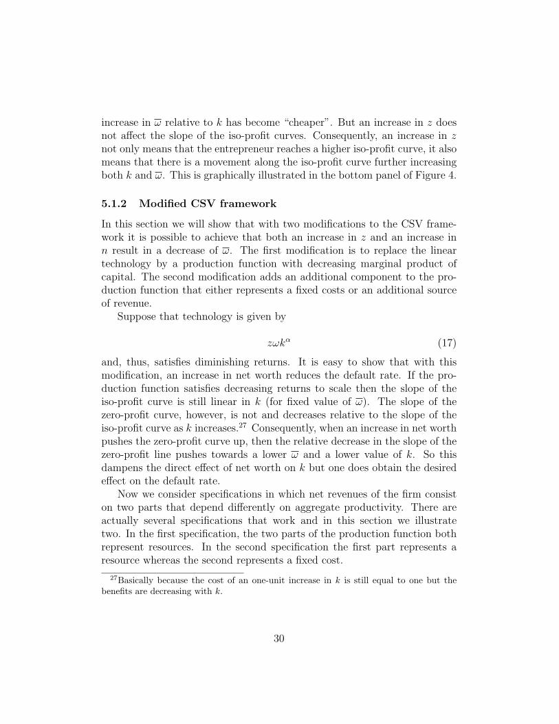
and, thus, satisfies diminishing returns. It is easy to show that with thismodification, an increase in net worth reduces the default rate. If the pro-duction function satisfies decreasing returns to scale then the slope of theiso-profit curve is still linear in k (for fixed value of ω). The slope of thezero-profit curve, however, is not and decreases relative to the slope of theiso-profit curve as k increases.27 Consequently, when an increase in net worthpushes the zero-profit curve up, then the relative decrease in the slope of thezero-profit line pushes towards a lower ω and a lower value of k. So thisdampens the direct effect of net worth on k but one does obtain the desiredeffect on the default rate.

Now we consider specifications in which net revenues of the firm consiston two parts that depend differently on aggregate productivity. There areactually several specifications that work and in this section we illustratetwo. In the first specification, the two parts of the production function bothrepresent resources. In the second specification the first part represents aresource whereas the second represents a fixed cost.

27Basically because the cost of an one-unit increase in k is still equal to one but thebenefits are decreasing with k.

30

Figure 5: Modified CSV Framework: Decreasing Returns to Scale

0

4

8

12

16

.0 .1 .2 .3 .4 .5 .6 .7

Default threshold

Zero-profit curve, n = 0.5Iso-profit curve, n = 0.5

Zero-profit curve, n = 1.5Iso-profit curve, n = 1.5

Size

of p

roje

ct

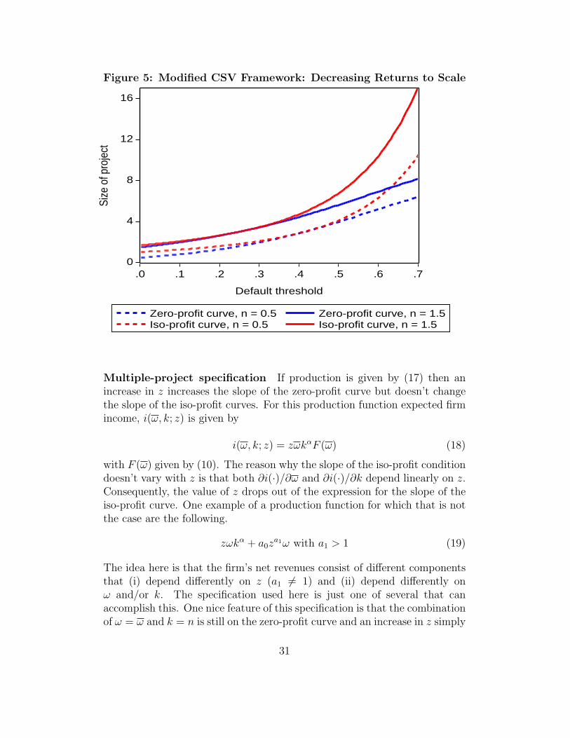
Multiple-project specification If production is given by (17) then anincrease in z increases the slope of the zero-profit curve but doesn’t changethe slope of the iso-profit curves. For this production function expected firmincome, i(ω, k; z) is given by

i(ω, k; z) = zωkαF (ω) (18)

with F (ω) given by (10). The reason why the slope of the iso-profit conditiondoesn’t vary with z is that both ∂i(·)/∂ω and ∂i(·)/∂k depend linearly on z.Consequently, the value of z drops out of the expression for the slope of theiso-profit curve. One example of a production function for which that is notthe case are the following.

zωkα + a0za1ω with a1 > 1 (19)

The idea here is that the firm’s net revenues consist of different componentsthat (i) depend differently on z (a1 6= 1) and (ii) depend differently onω and/or k. The specification used here is just one of several that canaccomplish this. One nice feature of this specification is that the combinationof ω = ω and k = n is still on the zero-profit curve and an increase in z simply

31

Figure 6: Modified CSV Framework: Multiple-Project Specifica-tion

0

1

2

3

4

5

6

.0 .1 .2 .3 .4 .5 .6

Default threshold

Zero-profit curve, z = 1.4Iso-profit curve, z = 1.4

Zero-profit curve, z = 1.5Iso-profit curve, z = 1.5

Size

of p

roje

ct

rotates the zero-profit curve upwards. But the increase in z also increasesthe slope of the iso-profit curves and it is easy to find values for a0 and a1

such that the default rate decreases. Figure 6 documents the effect of anincrease in z on the default rate and the capital lend when a0 is equal to 0.1and a1 is equal to 8.

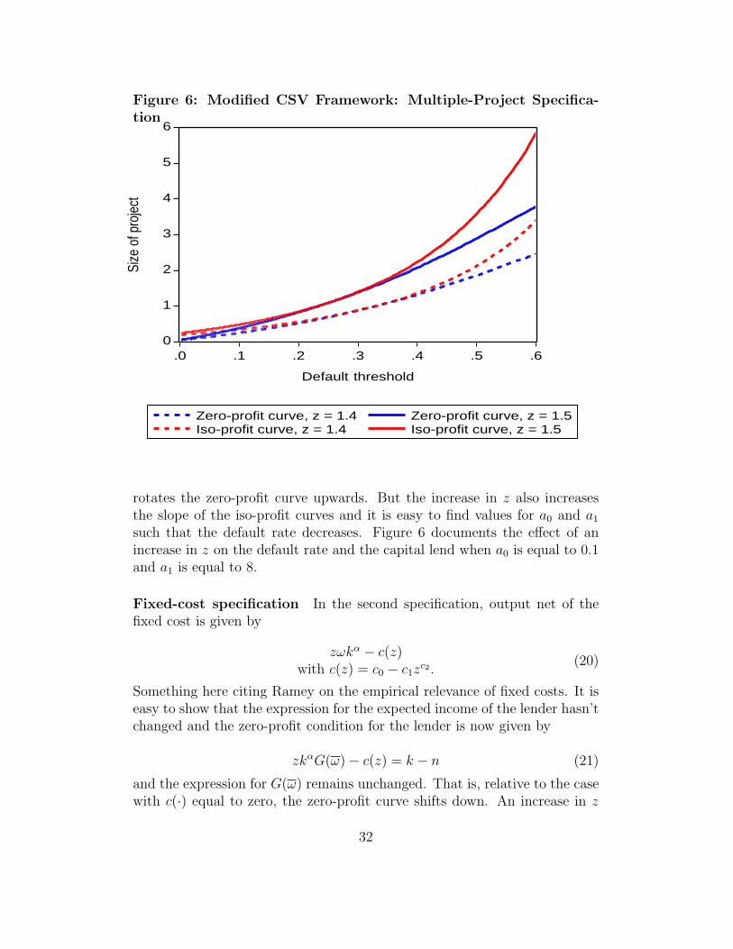
Fixed-cost specification In the second specification, output net of thefixed cost is given by

zωkα − c(z)with c(z) = c0 − c1z

c2 .(20)

Something here citing Ramey on the empirical relevance of fixed costs. It iseasy to show that the expression for the expected income of the lender hasn’tchanged and the zero-profit condition for the lender is now given by

zkαG(ω) − c(z) = k − n (21)

and the expression for G(ω) remains unchanged. That is, relative to the casewith c(·) equal to zero, the zero-profit curve shifts down. An increase in z

32

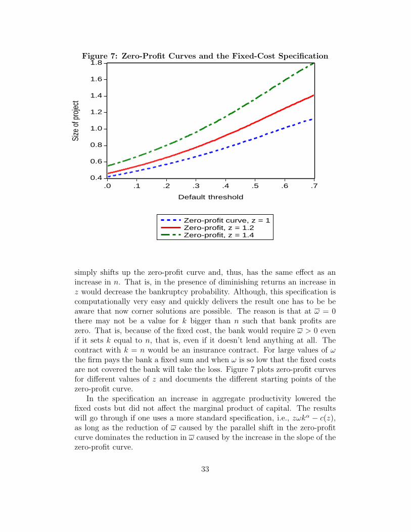
Figure 7: Zero-Profit Curves and the Fixed-Cost Specification

0.4

0.6

0.8

1.0

1.2

1.4

1.6

1.8

.0 .1 .2 .3 .4 .5 .6 .7

Default threshold

Zero-profit curve, z = 1Zero-profit, z = 1.2Zero-profit, z = 1.4

Size

of p

rojec

t

simply shifts up the zero-profit curve and, thus, has the same effect as anincrease in n. That is, in the presence of diminishing returns an increase inz would decrease the bankruptcy probability. Although, this specification iscomputationally very easy and quickly delivers the result one has to be beaware that now corner solutions are possible. The reason is that at ω = 0there may not be a value for k bigger than n such that bank profits arezero. That is, because of the fixed cost, the bank would require ω > 0 evenif it sets k equal to n, that is, even if it doesn’t lend anything at all. Thecontract with k = n would be an insurance contract. For large values of ωthe firm pays the bank a fixed sum and when ω is so low that the fixed costsare not covered the bank will take the loss. Figure 7 plots zero-profit curvesfor different values of z and documents the different starting points of thezero-profit curve.

In the specification an increase in aggregate productivity lowered thefixed costs but did not affect the marginal product of capital. The resultswill go through if one uses a more standard specification, i.e., zωkα − c(z),as long as the reduction of ω caused by the parallel shift in the zero-profitcurve dominates the reduction in ω caused by the increase in the slope of thezero-profit curve.

33

6 Complete Model

This section describes the full dynamic model. It consists of the following:(i) a unit mass of firms; (ii) a large number of competitive banks that provideone-period loans to firms; and (iii) a representative household which ownsthe firms.

6.1 Environment

Firm produce goods in this economy and are owned by the representativehousehold (shareholders). Firms can borrow funds from a bank, and at thesame time households also provide funds to the firm at an additional cost.Operating profits of the firm are given by

π(z, k) = zωf(k) − c(z), (22)

where z stands for aggregate productivity (with z > 0), ω for the i.i.d. idio-syncratic productivity shock (with ω > 0), and k for the firm’s capital stock.The term c(z) is a fixed cost contingent on the aggregate state. The capitalstock depreciates at rate δ. Further, assume that f(·) is continuously differ-entiable, strictly increasing, strictly concave with f(0) = 0, and satisfyingthe Inada conditions.

The timing assumptions are as follows. The debt contract is written atthe beginning of the period at which point the value of z is known. The valueof the idiosyncratic shock, ω, is observed at the end of the period. We assumethat at that point next period’s value of the aggregate shock, z′, is known aswell. The firm then makes the default decision. If the firm continues thenthe shareholders decide whether to liquidate the firm (take all resources outof the firm), pay out any dividends, or add additional equity to the firm.

6.2 Debt choice

This economy is populated by a large number of banks that lend funds tofirms in a competitive market. Consequently, banks make zero expected prof-its on each loan they make to a firm. We assume that banks have unlimitedaccess to funds. Below we describe the environment under two possible sce-narios. Under the first scenario, firms defaults if the resources in the firmare not enough to pay back the amount borrowed plus interest. This ignoresfuture earnings potential, or continuation value, as an asset of the firm. This

34

assumption would be appropriate if adding equity to a firm in distress isprohibitively costly. Under the second scenario the firm defaults if, afterrepayment of the debt, the continuation value of the firm is negative. It isthen possible that a firm that doesn’t have enough resources to repay thedebt will not default because the future earnings potential of the firm is at-tractive enough to acquire additional equity (and cover the costs of obtainingadditional equity).

6.2.1 Without Valuation Effects

At the beginning of the period the firm borrows (k−n) from one of the banks,where n is the firm’s net worth. The firm agrees to repay (1 + rb)(k − n) atthe end of the period. Although we allow the firm to issue equity we assumethat the costs are prohibitively expensive when the firm is in distress. Thefirm then defaults if ω is less than the default threshold, ω̄, where ω̄ satisfies

zω̄kα + (1 − δ)k − c(z) = (1 + rb)(k − n). (23)

If the firm defaults the bank gets

zωkα + (1 − δ)k − c(z) − µ(1 + rb)(k − n), (24)

where µ represent bankruptcy costs, which are assumed to be a fraction ofthe contracted repayment value of the debt. Let Φ(ω) be the cumulativedistribution function of the idiosyncratic shock. We can write the expectedincome of the bank for each loan it issues as∫ ω̄

0

[zωkα + (1− δ)k − c(z)] dΦ(ω) + [1− (1 + µ)Φ(ω̄)](1 + rb)(k − n). (25)

As in the static case, the financial contract is given by the (k, ω̄) pair thatmaximizes the firm’s value subject to the lender being indifferent betweenloaning the funds or retaining them.

maxk,ω̄

∫ ∞

ω̄

E[v(z′, x)|z]dΦ

s.t. x = zωkα + (1 − δ)k − c(z) − (1 + rb)(k − n), (26)

zkαG(ω̄) + (1 − µΦ(ω̄))[(1 − δ)k − c(z)] > (k − n).

35

where

G(ω̄) = [1 − (1 + µ)Φ(ω̄)]ω̄ +

∫ ω̄

0

ω dΦ. (27)

Note that we assume that the opportunity cost for the bank is equal tozero. The function v(z′, x) represent the value of the firm at the end of theperiod when next period’s aggregate shock is equal to z′ and resources withinthe firm are equal to x. This continuation value takes into account that atthe end of the period the firm could liquidate the firm (v(z′, x) = x), issuedividends (n′ < x), or add additional equity (n′ > x).

Furthermore, the participation constraint of the firm must hold as well. Inparticular we need that the maximized value in expression (26) to be greateror equal to E[v(z′, n)|z]. This condition will always be satisfied below. Whenthe lending contract is designed the firm has already decided that it isn’tworth liquidating the firm. Because of the fixed cost, however, it may stillbe better for the firm to produce without a bank contract and set k equal ton. Thus, we have to check the participation constraint that the maximizedvalue in expression (26) to be greater or equal to E[v(z′, n)|z]. We neverfound this constraint to be violated.

Further, from the financial contract we can simplify expression (26) usingthe definition of the default threshold given in (23):

x = z(ω − ω̄)kα. (28)

6.2.2 With Valuation Effects

We now consider the case where v(0, z′) > 0. Obviously, this would mean thatit is worthwhile for the firm to add equity, which would require that issuingequity for a distressed firm is not prohibitively expensive. The maximumamount of equity an entrepreneur is willing to add to the firm is given by theamount −x(z′) > 0, where x(z′) satisfies

v(x(z′), z′) = 0. (29)

The firm will now default when ω < ω, where ω satisfies

zωkα + (1 − δ)k − c(z) − x(z′) = (1 + rb)(k − n). (30)

We assume that when ω < ω and the firm, thus, cannot raise enoughequity to pay back the debt that part of the bankruptcy costs are that the

36

value of the firm is equal to zero.28 In case default occurs the bank thenreceives the cash in the firm and pays the bankruptcy cost

zωkα + (1 − δ)k − c(z) − µ(1 + rb)(k − n). (31)

We can then re-write the bank’s expected revenues as

E

[ ∫ ω(z′)

0[zωkα + (1 − δ)k − c(z)] dΦ(ω)

+[1 − (1 + µ)Φ(ω(z′))](1 + rb)(k − n)

∣∣∣∣ z

](32)

Note that with valuation effects on the default decision the bank makeszero-expected profits ex-ante but not ex-post, depending on the realizationof next period’s aggregate productivity. Hence, the profits of banks, Π couldbe either positive or negative. Given values of n and z, the financial contractspecifies a debt amount k − n, and a lending rate rb, such that:

maxk,ω̄

E

[∫ ∞

ω(z′)

v(z′, x)d Φ(ω)

∣∣∣∣ z

](33)

s.t. x = zkα(ω − ω(z′)) + x(z′), (34)

and (32). (35)

6.3 Equity choice

In addition to debt financing the firm can also attract outside equity. Toconsider a more realistic and interesting equilibrium in which both debt andequity co-exist, we assume firms face a linear-quadratic cost of issuing equity.This cost function captures both the cost of underwriting fees and possibleadverse selection problems in equity markets. More specifically, the cost ofexternal equity is defined as:

λ = λ(e; z′) ≥ 0, (36)

where e is new equity issued. When e < 0 then the firm issues dividends andwe assume that in that case λ(·) is equal to zero. Furthermore, we assumethat λ(0; z′) = λ′(0; z′) and when e > 0 that λ(e; z′) > 0 and λ′(e; z′) > 0.We allow for the possibility that the cost of issuing equity is decreasing with

28This means that when ω < ω there is no point for the bank to lower the debt obligationso that additional equity can be attracted.

37

z′. The idea would be that an increase in z′ increases the bargaining positionof existing shareholders and makes it easier to attract new equity. Recallthat we assume that the firm observes next period productivity, z′, before itdecides how much equity to issue in the current period.

Recall that v(z′, x) is the optimal value of a firm before issuing equitywhen next period’s productivity is z′ and with cash-on-hand equal to x.The firm’s optimization problem can be specified in terms of the followingdynamic programming problem:

v(z′, x) = maxe,n′

−e− λ(e, z′) + w(z′, n′) (37)

s.t. − e + n′ = x, (38)

where w(z′, n′) is the firm’s optimal value after the equity decision is made.Note that the firm can set −e = x, that is n′ = 0. In this case the firm isliquidated and v(z′, x) = x. We focus on the case where v(z′, 0) > 0 andit is worthwhile to issue equity even when there is no net worth in the firm.Then liquidation never happens. The reason is that if a firm issues equitythe slope of w(·) must be strictly greater than one (to cover the issuancecost). As n′ increases the slope of w(·) decreases but never gets below one,29

consequently we always have that w(z′, n′) > n′.This value function is defined as follows:

w(z′, n′) =1

1 + rE

[∫ ∞

ω̄′v(z′′, x′) dΦ(ω)|z′

]. (39)

Finally, we define the firm’s next period cash-on-hand, x′, as follows:

x′ =

{0 if ω < ω̄′,

z′ω′k′α + (1 − δ)k′ − c(z′) − (1 + r′b)(k′ − n′) if ω > ω̄′.

(40)

Bank loans in our model are within-period loans and the opportunitycosts is equal to zero. The discount rate is strictly bigger than zero. Ifinstead we would assume that the opportunity cost for banks is equal to r,then firms would never pay out dividends. Because of diminishing returnsthere would be a maximum level of capital but firms would keep funds insidethe firm even if net worth would exceed that level. Firms would simply investthe excess funds at rate r which is the same as what it would earn outside

29The slope will be equal to one when it starts paying out dividends.

38

the relationship, but keeping funds inside the firm serves as a buffer againstdrops in net worth (and avoiding paying issuance costs). Alternatively, wecould assume that the opportunity costs for the banks is equal to r but thatfunds deposited by the firm at the bank earn less than r.

6.4 Household problem

In this economy there is a representative household which receives an endow-ment w and uses it to purchase consumption and shares of firms. Householdsmaximize the expected lifetime utility derived from consumption:

E0

∞∑t=0

βtct, (41)

where 0 < β = 1/(1 + r) < 1 is the discount factor. The household incomecomes from two sources: exogenous income and the dividends of firms. Thehousehold’s budget constraint can be written as:

c +

∫s′(z′, x)p(z′, x) dΓ(z′, x) = w +

∫s(z′, x)p(z′, x) d Γ(z′, x)

+

∫s′(z′, x)d(z′, x) dΓ(z′, x) + Π, (42)

where s(z′, x) stands for the fraction of shares owned by the household,p(z′, x) for the price of the share and d(z′, x) for the dividend. The prof-its of banks are denoted by Π. As in Gomes (2001) we assume the paymentof dividends occurs right after the shares of the firm are bought.

Taking first-order conditions w.r.t. the accumulation of shares we get:

p(z′, x) = d(z′, x) + βE[p(z′′, x′)|z′]. (43)

where d(z′, x) = −e(z′, x) − λ(e, z′).

Proposition 1 In equilibrium p(z′, x) = v(z′, x).

39

7 Results

A Appendix

A.1 Kocherlakota (2000)

Kocherlakota (2000) argues that the collateral approach cannot deliver largeeffects for reasonable parameter values. Here we want to point out that thisis true in the framework he considers but the framework of Kocherlakota isquite different from the KM framework. In particular, Kocherlakota assumesthat the constrained agents are the only ones that hold the fixed factor.Consequently, there is no reallocation of the fixed factor from less productiveto more productive agents as in KM. Whereas in KM the amount of thefixed factor held by constrained agents is the center piece of the analysis,in Kocherlakota it is the investment in the uncollaterizable investment. Butthis investment is not subject to the leverage effect discussed in the maintext. Moreover, it is also not affected by changes in the current value ofland. To see why consider the borrowing constraint (assumed to be binding)and the budget constraint used by Kocherlakota.

(1 + rl)b = q′k (44)

qk + x = n + b (45)

where x is the amount of uncollaterizable investment. In the Kocherlakotaframework farmers use all the land so that k is constant and equal to thegiven supply of the aggregate factor. Suppose the aggregate supply is equalto 1. The solution for x is then given by

x = profits− (1 + rl)b−1 + q′(1 + r′). (46)

Note that the leverage effect has disappeared. The direct effect of a change innet worth on investment is equal to one whereas in KM it is huge. Also, notethat the current-period land price has disappeared from this equation. InKM an increase in q increases n which has such a huge effect on b (becauseof the leverage effect) that this effect dominates the downward effect on bcaused by the decrease in q′/q (keeping q′ constant).

40

References

Albuquerque, R., and H. Hopenhayn (2004): “Optimal Lending Con-tracts and Firm Dynamics,” The Review of Economic Studies, 71, 285–315.

Bernanke, B., M. Gertler, and S. Gilchrist (1999): The Finan-cial Accelerator in a Quantitative Business Cycle Frameworkchap. 21, pp.1341–1393. Elsevier Science B.V.

Bernanke, B. S., J. Y. Campbell, and T. M. Whited (1990): “U.S.Corporate Leverage: Developments in 1987 and 1988,” Brookings Paperson Economic Activity, 1, 255–286.

Carlstrom, C. T., and T. S. Fuerst (1997): “Agency Costs, Net Worth,and Business Fluctuations: A Computable General Equilibrium Analysis,”American Economic Review, 87, 893–910.

(1998): “Agency Costs and Business Cycles,” Economic Theory,12, 583–597.

Cooley, T., R. Marimon, and V. Quadrini (2004): “Aggregate Conse-quences of Limited Contract Enforceability,” Journal of Political Economy,112, 817–847, NBER working paper 10132.

Cooley, T., and V. Quadrini (2001): “Financial Markets and Firm Dy-namics,” American Economic Review, 91, 1286–1310.

(2005): “Monetary Policy and Financial Decisions of Firms,” Eco-nomic Theory, 27, 243–270.

Cordoba, J. C., and M. Ripoll (2004): “Credit Cycles Redux,” Inter-national Economic Review, 45, 1011–1046.

Covas, F. (2004): “Risk-Taking Executives, the Value of the Firm andEconomic Performance,” mimeo.

den Haan, W. J., G. Ramey, and J. Watson (2000): “Job Destructionand Propagation of Shocks,” American Economic Review, 90, 482–498.

(2003): “Liquidity Flows and Fragility of Business Enterprises,”Journal of Monetary Economics, 50, 1215–1241.

41

Fama, E. F., and K. R. French (2005): “Financing Decisions: WhoIssues Stock?,” Journal of Financial Economics, 76, 549–582.

Frank, M. Z., and V. K. Goyal (2003): “Testing the Pecking OrderTheory of Capital Structure,” Journal of Financial Economics, 67, 217–248.

Gande, A., M. Puri, and A. Saunders (1999): “Bank Entry, Competi-tion, and the Market for Corporate Securities Underwriting,” Journal ofFinancial Economics, 54, 165–195.

Gomes, J. F. (2001): “Financing Investment,” American Economic Review,91, 1263–1285.

Hennessy, C. A., and T. M. Whited (2005): “Beyond Investment-CashFlow Sensitivities: Using Indirect Inference to Estimate the Cost of Ex-ternal Funds,” mimeo.

Kiyotaki, N., and J. Moore (1997): “Credit Cycles,” Journal of PoliticalEconomy, 105, 211–248.

Kocherlakota, N. R. (2000): “Creating Business Cycles Through CreditConstraints,” Federal Reserve Bank of Minneapolis Quarterly Review, 24,2–10.

Moyen, N. (2004): “Investment-Cash-Flow Sensitivities: Constrained ver-sus Unconstrained Firms,” Journal of Finance, 59, 2061–2091.

Quadrini, V. (2004): “Investment and Liquidation in Renegotiation-ProofContracts with Moral Hazard,” Journal of Monetary Economics, 51, 713–751.

Townsend, R. M. (1979): “Optimal Contracts and Competitive Marketswith Costly State Verification,” Journal of Economic Theory, 21, 265–293.

42