34
The role of energy in the mitigation of (and adaptation to) climate change Pedro Linares BC3 Summer School San Sebastian, July 15th 2014
| Date post: | 10-Aug-2015 |
| Category: |
Environment |
| Upload: | bc3-basque-center-for-climate-change |
| View: | 20 times |
| Download: | 0 times |

The role of energy in the mitigation of (and adaptation to) climate change
Pedro Linares
BC3 Summer School
San Sebastian, July 15th 2014

1 / 32
The role of energy in GHG emissions (I) Final�Draft� Technical�Summary� IPCC�WGIII�AR5��
14�of�99��
�
�Figure TS.3. Allocation of GHG emissions across sectors and country income groups. Panel a: Share (in %) of direct GHG emissions in 2010 across the sectors. Indirect CO2 emission shares from electricity and heat production are attributed to sectors of final energy use. Panel b: Shares (in %) of direct and indirect emissions in 2010 by major economic sectors with CO2 emissions from electricity and heat production attributed to the sectors of final energy use. Lower panel: Total anthropogenic GHG emissions in 1970, 1990 and 2010 by economic sectors and country income groups. GHG emissions from international transportation are reported separately. The emissions data from Agriculture, Forestry and Other Land Use (AFOLU) includes land-based CO2 emissions from forest and peat fires and decay that approximate to net CO2 flux from the Forestry and Other Land Use (FOLU) sub-sector as described in chapter 11 of this report. Emissions are converted into CO2-
IPCC AR5, WG3 Technical Summary

2 / 32
The role of energy in GHG emissions (II)
3 / 32
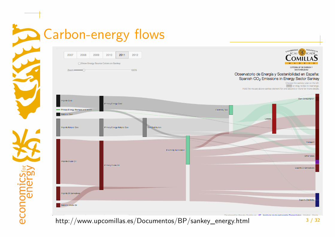
Carbon-energy flows
http://www.upcomillas.es/Documentos/BP/sankey_energy.html

4 / 32
The role of energy in mitigation • Reaching atmospheric concentration levels of 430 to 650
ppm by 2100 will require large-scale challenges to global and energy systems over the coming decades [high confidence] – 3x – 4x share low-carbon energy in 2050 – 2100 concentration levels unachievable if the full suite of low-carbon technologies is not available
– Demand reductions on their own will not be sufficient – But will be a key mitigation strategy and will affect the scale of the mitigation challenge for the energy supply side
(AR5 WG3 Technical Summary)

5 / 32
Drivers for GHG emissions (I)
Final�Draft� Technical�Summary� IPCC�WGIII�AR5��
18�of�99��
TS.2.2��� Greenhouse�gas�emission�drivers�
This�section�examines�the�factors�that�have,�historically,�been�associated�with�changes�in�emission�levels.�Typically,�such�analysis�is�based�on�a�decomposition�of�total�emissions�into�various�components��such�as�growth�in�the�economy�(GDP/capita),�growth�in�the�population�(capita),�the�energy�intensity�needed�per�unit�of�economic�output�(energy/GDP)�and�the�emission�intensity�of�that�energy�(GHGs/energy).�As�a�practical�matter,�due�to�data�limitations�and�the�fact�that�most�GHG�emissions�take�the�form�of�CO2�from�industry�and�energy,�almost�all�this�research�focuses�on�CO2�from�those�sectors.�
Growth�in�economic�output�and�population�are�the�two�main�drivers�for�worldwide�increasing�GHG�emissions,�outpacing�emission�reductions�from�improvements��in�energy�intensity�(high�confidence).�Worldwide�population�increased�by�86%�between�1970�and�2010,�from�3.7�to�6.9�billion.�Over�the�same�period,�economic�growth�as�measured�through�production�and/or�consumption�has�also�grown�a�comparable�amount,�although�the�exact�measurement�of�global�economic�growth�is�difficult�because�countries�use�different�currencies�and�converting�individual�national�economic�figures�into�global�totals�can�be�done�in�various�ways.��With�rising�population�and�economic�output,�emissions�of�CO2�from�fossil�fuel�combustion�have�risen�as�well.�Over�the�last�decade�the�importance�of�economic�growth�as�a�driver�of�global�emissions�has�risen�sharply�while�population�growth�has�remained�roughly�steady.�Due�to�technology,�changes�in�the�economic�structure,�the�mix�of�energy�sources�and�changes�in�other�inputs�such�as�capital�and�labour,�the�energy�intensity�of�economic�output�has�steadily�declined�worldwide,�and�that�decline�has�had�an�offsetting�effect�on�global�emissions�that�is�nearly�of�the�same�magnitude�as�growth�in�population�(Figure�TS.6).�There�are�only�a�few�countries�that�combine�economic�growth�and�decreasing�territorial�emissions�over�longer�periods�of�time.�Decoupling�remains�largely�atypical,�especially�when�considering�consumptionͲbased�emissions.�[1.3,�5.3]�
�Figure TS.6.�Decomposition of decadal absolute changes in total CO2 emissions from fossil fuel combustion by Kaya factors: population (blue), GDP per capita (red), energy intensity of GDP (green) and carbon intensity of energy (purple). Total decadal changes in CO2 emissions are indicated by a black triangle. Changes are measured in gigatonnes of CO2 emissions per year (Gt/yr). [Figure 1.7]
IPCC AR5, WG3 Technical Summary

6 / 32
Drivers for GHG emissions (II) Final�Draft� Technical�Summary� IPCC�WGIII�AR5��
20�of�99��
�Figure TS.7.�Global baseline projection ranges for Kaya factors. Scenarios harmonized with respect to a particular factor are depicted with individual lines. Other scenarios depicted as a range with median emboldened; shading reflects interquartile range (darkest), 5th – 95th percentile range (lighter), and full extremes (lightest), excluding one indicated outlier in population panel. Scenarios are filtered by model and study for each indicator to include only unique projections. Model projections and historic data are normalized to 1 in 2010. GDP is aggregated using base-year market exchange rates. Energy and carbon intensity are measured with respect to total primary energy. [Figure 6.1]
IPCC AR5, WG3 Technical Summary

7 / 32
Access to energy?
these emissions on global warming as measured by the increase in surface global mean temperature. The table shows that the cumulative emissions due to energy poverty eradication would be in the range of 16 to 131 GtCO2, with the discrepancy mostly attributable to the use and retirement of the additional energy infrastructure in the long term. In terms of consequences for global warming, the induced temperature change would be very limited, below 0.1C in all cases with high probability7. It is also instructive to compare this level of emissions to the carbon budget consistent with policies aimed at climate stabilization; climate stabilization policies compatible with the 2 degree Celsius objective entail cumulative emissions over the century in the range of 1500-2500 GtCO2, and thus the emissions associated with the energy poverty policy would increase the mitigation effort by at most less than 10%. Carbon prices for a 2C climate policy (e.g. 450 ppm-eq) have been estimates at 12-120 $/tCO2 in net present value, with a median of around 40$/tCO2; taking this last value the carbon costs of the energy eradication programme would be at most in the order of 5 USD Trillions (for the high scenario of 131 GtCO2). These do not represent real economic costs, but only the value of the emissions at the marginal price of carbon consistent with the 2C policies. Economy wide costs are likely to be lower. It is however worth noticing that the economic costs of emissions reductions as predicted by the integrated assessment models which have run climate stabilization scenarios are very non linear in the mitigation effort (Clarke et al., 2009): thus, even a mild increase in mitigation effort could lead to a non marginal change in the policy costs, but only in case of already stringent climate targets.
Low High
Optimistic Pessimistic Optimistic Pessimistic
2009-2030: Energy poverty alleviation emissions (GtCO2)
2.9 2.9 17.8 17.8
2030-2060: Use of additional energy infrastructure (GtCO2)
7.9 7.9 48.5 48.5
2060-2100: Retirement of additional infrastructure (GtCO2)
5.3 10.5 32.3 64.7
2009-2100: Total emissions (GtCO2) 16.1 21.3 98.7 131
Additional temperature increase (degree C): mean and 10-90 percentile in square brackets
0.008
[0.004-0.011]
0.01
[0.006-0.014]
0.047
[0.027-0.067]
0.063
[0.036-0.089]
Table 3: Estimated additional emissions and temperature rise from an energy poverty alleviation program.
Concluding remarks
7 We use the carbon budget approach which relates every 1000GtCO2 emitted in the atmosphere with an increase in
equilibrium temperature of 0.48C, with a 90% range of 0.27C to 0.68C.
Chakravarty and Tavoni, 2013

8 / 32
Energy-related mitigation options • Decarbonization of energy supply • Final energy demand reductions • Switch to low-carbon fuels • Different by sector
– Decarbonization of electricity generation is a key component: quicker and simpler
– The transport sector is difficult to decarbonize, and opportunities for fuel switching are low in the short term
– Large achievable potential in the building sector, but strong barriers

9 / 32
Mitigation potential
Final�Draft� Technical�Summary� IPCC�WGIII�AR5��
43�of�99��
carriers�compared�to�buildings�and�industry�(Figure�TS.17).�[6.3.4,�6.8,�8.9,�9.8,�10.10,�7.11,�Figure�6.17]
The�availability�of�carbon�dioxide�removal�technologies�affects�the�size�of�the�mitigation�challenge�for�the�energy�endͲuse�sectors�(robust�evidence,�high�agreement)�[6.8,�7.11].�There�are�strong�interdependencies�between�the�required�pace�of�decarbonization�of�energy�supply�and�endͲuse�sectors.�The�more�rapid�decarbonization�of�supply�generally�provides�more�flexibility�for�the�endͲuse�sectors.�However,�barriers�to�decarbonizing�the�supply�side,�resulting�for�example�from�a�limited�availability�of�CCS�to�achieve�negative�emissions�when�combined�with�bioenergy,�require�a�more�rapid�and�pervasive�decarbonisation�of�the�energy�endͲuse�sectors�in�scenarios�achieving�low�CO2eq�concentration�levels�(Figure�TS.17).�The�availability�of�mature�largeͲscale�energy�generation�or�carbon�sequestration�technologies�in�the�AFOLU�sector�also�provides�flexibility�for�the�development�of�mitigation�technologies�in�the�energy�supply�and�energy�endͲuse�sectors�[11.3]�(limited�evidence,�medium�agreement),�though�there�may�be�adverse�impacts�on�sustainable�development.��
Figure TS.17. Direct emissions of CO2 and non-CO2 GHGs across sectors in mitigation scenarios that reach around 450 (430-480) ppm CO2eq concentrations in 2100 with using CCS (left panel) and without using CCS (right panel). The numbers at the bottom of the graphs refer to the number of scenarios included in the ranges that differ across sectors and time due to different sectoral resolution and time horizon of models. [Figures 6.35]
Spatial�planning�can�contribute�to�managing�the�development�of�new�infrastructure�and�increasing�systemͲwide�efficiencies�across�sectors�(robust�evidence,�high�agreement).�Land�use,�transport�choice,�housing,�and�behaviour�are�strongly�interlinked�and�shaped�by�infrastructure�and�urban�form.��Spatial�and�land�use�planning,�such�as�mixed�use�zoning,�transportͲoriented�development,�increasing�density,�and�coͲlocating�jobs�and�homes�can�contribute�to�mitigation�across�sectors�by�a)�reducing�emissions�from�travel�demand�for�both�work�and�leisure,�and�enabling�nonͲmotorized�transport,�b)�reducing�floor�space�for�housing,�and�hence�c)�reducing�overall�direct�and�indirect�energy�use�through�efficient�infrastructure�supply.�Compact�and�inͲfill�development�of�urban�spaces�and�intelligent�densification�can�save�land�for�agriculture�and�bioenergy�and�preserve�land�carbon�stocks.�[8.4,�9.10,�10.5,�11.10,�12.2,�12.3]��
Interdependencies�exist�between�adaptation�and�mitigation�at�the�sectoral�level�and�there�are�benefits�from�considering�adaptation�and�mitigation�in�concert�(medium�evidence,�high�agreement).�Particular�mitigation�actions�can�affect�sectoral�climate�vulnerability,�both�by�
IPCC AR5, WG3 Technical Summary

10 / 32
The INDC Scenario (I)
38 World Energy Outlook | Special Report
reaching a plateau by around 2020 but there are differing trends across OECD and
non-OECD regions, with the former declining and the latter continuing to increase. lobal emissions from coal use increase only slightly, relative to today, and are around
14.5 t in 2030. lobal oil demand reaches million barrels per day (mb d) in 2030, around % higher than today, with actions in the INDC cenario helping to slow demand growth in the transport sector. World natural gas demand increases by around 30% by 2030, helping to suppress growth in emissions when acting as a substitute for other fossil fuels but adding to emissions when acting as a substitute for renewables and nuclear. By 2030, coal accounts for 41% of energy-related CO2 emissions, oil for 34% and natural gas for 25%. While significant hydropower potential remains in some regions, the global expansion of hydropower capacity is relatively modest. olar and wind capacity increase more rapidly. All low-carbon options collectively account for around one- uarter of primary energy demand in 2030.
Figure 2.2 ⊳ Global primary energy demand by type in the INDC Scenario
3 000
6 000
9 000
12 000
15 000
18 000
2000 2005 2010 2013 2020 2025 2030
Mto
e
5%
10%
15%
20%
25%
30% Other renewables
Bioenergy
Hydro
Nuclear
Gas
Oil
Coal Share of low-carbon sources (right axis)
Note: Other renewables includes wind, solar (photovoltaic and concentrating solar power), geothermal, and marine.
The pro ected path for energy-related emissions in the INDC cenario means that, based on IPCC estimates, the world s remaining carbon budget consistent with a 50% chance of keeping a temperature increase of below 2 °C would be exhausted around 2040, adding a grace period of only around eight months, compared to the date at which the budget would be exhausted in the absence of INDCs ( igure 2.3). This date is already within the lifetime of many existing energy sector assets: fossil-fuelled power plants o en operate for 30-40 years or more, while existing fossil-fuel resources could, if all developed, sustain production levels far beyond 2040. If energy sector investors believed that not only new investments but also existing fossil-fuel operations would be halted at that critical point, this would have a profound effect on investment even today.
IEA WEO Special Report on Energy and Climate, 2015

11 / 32
The INDC Scenario (II)
40 World Energy Outlook | Special Report
per kilometre improve significantly by 2030, the latter declining by around half. Despite these improvements, the transport sector accounts for nearly half of the pro ected increase in global energy-related CO2 emissions to 2030. Oil consumption in the sector goes from 4 mb d in 2013 to 5 mb d in 2030, while the transition towards alternative vehicles is barely underway in the INDC cenario and continues to face a number of challenges relating to costs, refuelling infrastructure and consumer preferences. ( ee Chapter 4 for more on electric vehicles.)
Neither the scale nor the composition of energy sector investment in the INDC cenario is suited to move the world onto a 2 °C path. Cumulative investment in fossil-fuel supply accounts for close to 45% of the energy sector total, while low-carbon energy supply accounts for 15% ( igure 2.4). lobal investment in fossil-fuelled power generation capacity declines over time, to stand at around 100 billion in 2030, but investment in coal-fired plants still accounts for more than half of the total at that time. Investment in renewable-based power supply remains relatively stable over the period to 2030, averaging 2 0 billion per year, with ongoing reductions in unit costs masking higher levels of deployment. lobal investment in nuclear power remains concentrated in ust a few markets. On the demand side, around trillion is invested in energy efficiency from 2015 to 2030 in the INDC cenario.3 One-third of this is spent by motorists on more efficient cars, while more than another third is on improved efficiency in buildings (mainly insulation, efficient appliances and lighting) and the rest is split between energy efficiency in industry and road freight.
Figure 2.4 ⊳ Cumulative global energy sector investments by sector in the INDC and 450 Scenarios, 2015-2030 (trillion dollars, 2013)
0.7
4.4
3.0
1.7 0.9
4.2
5.0
9.3
5.7
0.7 0.2
INDC Scenario $35.8 trillion
1.1
5.5
4.6
1.9 1.3
5.6 4.2
7.6
5.2
0.6 0.4
450 Scenario $37.9 trillion
End-use eĸciency: Industry Transport Buildings
Fuel supply:
Biofuels Coal Gas Oil
Power supply:
Nuclear Renewables T&D
Fossil fuels
Note: T D is transmission and distribution.
3. Energy efficiency investment is defined as the additional expenditure made by energy users to improve the performance of their energy-using e uipment above the average efficiency level of that e uipment in 2012.
IEA WEO Special Report on Energy and Climate, 2015

12 / 32
The IEA bridge to 2ºC (I)
74 World Energy Outlook | Special Report
E i ion tren in t e ri ge cenario
oba emissions abatement
Effective implementation of the proposed measures in the Bridge cenario would have profound implications for global emissions.8 Emissions would be 2. t (or %) lower than in the INDC cenario by 2025 and 4. t (or 13%) lower by 2030, meaning that energy-related emissions would peak and then begin to decline by around 2020 ( igure 3.2). Their adoption is insufficient alone to put the world on track for reaching the 2 °C target (the long-term global mean temperature would rise by 2. °C if no additional mitigation measures were taken later), but they would put the world on track for further emissions reductions. They would also lock-in recent trends that decouple economic growth from emissions growth in some regions and broaden that de-linking ( igure 3.3).
Figure 3.2 ⊳ Global energy-related GHG emissions reduction by policy measure in the Bridge Scenario relative to the INDC Scenario
32
34
35
36
37
38
2014 2020 2025 2030
Bridge Scenario
INDC Scenario
Fossil-fuel subsidy reform
Upstream methane reductions
Renewables investment Reducing ine cient coal
Energy e ciency
Gt C
O2-e
q
10%
9%
49%
17%
15%
33
The largest contribution to global GHG abatement comes from energy efficiency, which is responsible for 4 % of the savings in 2030 (including direct savings from reduced fossil-fuel demand and indirect savings as a result of lower electricity demand thereby reducing emissions from the power generation).9 The power sector is the second-largest contributor to global savings, at 2 % in 2030. While limitations on the use of the least-efficient coal power plants are effective in curbing global GHG emissions until 2020
. Tables containing detailed pro ection results for the Bridge cenario by region, fuel and sector are available in Annex B.
. The results take into account direct rebound effects as modelled in the IEA s World Energy odel. Direct rebound effects are those in which energy efficiency increases the energy service gained from each unit of final energy, reducing the price of the service and eventually leading to higher consumption. Policies to increase end-user prices are one way to reduce such rebound effects, but are not considered in the Bridge Scenario (except for fossil-fuel subsidy reform). The level of the rebound effect is very controversial; a review of 500 studies suggests though that direct rebound effects are likely to be over 10% and could be considerably higher (IPCC, 2014).
IEA WEO Special Report on Energy and Climate, 2015

13 / 32
The IEA bridge to 2ºC (II)
76 World Energy Outlook | Special Report
Figure 3.4 ⊳ Energy-related GHG emissions reduction in CO2-eq terms by policy measure and region in the Bridge Scenario relative to the INDC Scenario, 2030
20% 40% 60% 80% 100%
China
Middle East
India
United States
Southeast Asia
Russia
Africa
Latin America
European Union
Efficiency Renewables Inefficient coal-fired power plants
Fossil-fuel subsidies
Upstream methane reductions
1 346 Mt
553 Mt
395 Mt
362 Mt
302 Mt
280 Mt
260 Mt
247 Mt
213 Mt
Notes: The relative shares of emissions savings by policy measure have been calculated using a ogarithmic ean Divisia Index I ( DI I) decomposition techni ue. In regions where fossil-fuel subsidies hinder energy efficiency investments today, the existing subsidy level in each sector was used to quantify the impact of fossil-fuel subsidy reform on emissions savings.
Although the strong growth in energy demand in China over the past decade has locked-in a relatively carbon-intensive energy infrastructure, an earlier peak in CO2 emissions (including process emissions) can be achieved than in the INDC cenario: in the Bridge
cenario, it is achieved in the early 2020s, as China s carbon intensity (i.e. the amount of CO2 emitted per unit of gross domestic product DP ) drops by 5.4% per year between 2013 and 2030, compared with 4. % in the INDC cenario. The share of non-fossil fuels in primary energy demand rises to 23%10 by 2030, three percentage points above the target in the INDC cenario. In India, planned energy sector policies have a focus on large-scale solar P deployment. aking more use of the energy efficiency potential across all sectors could help to cost-effectively reach India s energy sector targets and support a total reduction of GHG emissions by 400 Mt CO2-e (or 11%) in 2030, relative to the INDC cenario.
As in the case of China and India, most other countries had not submitted their INDCs for COP21 by 14 ay 2015, but their existing and planned policies give a good indication of the likely level of ambition of their targets. In Japan, for example, the existing and announced
10. alue is calculated using the coal-e uivalent approach in Chinese statistics, which is likely to be the basis of the Chinese INDC. Using IEA definitions, the share of non-fossil fuels is 20% in 2030 in the Bridge cenario.
IEA WEO Special Report on Energy and Climate, 2015

14 / 32
Assessing costs and potentials • It is easy to overestimate potentials and underestimate costs – Counterfactual scenarios – Public vs Private perspectives
• Discount rates • Taxes
– Interactions between options – Rebound effect – Bottom-up vs Top-down

15 / 32
The McKinsey curve
6 / 14
The McKinsey curve

16 / 32
AR5 Energy supply
Final�Draft� Technical�Summary� IPCC�WGIII�AR5��
� 48�of�99�� ��
Figure TS.19. Specific direct and lifecycle emissions (gCO2/kWh and gCO2eq/kWh, respectively) and levelized cost of electricity (LCOE in USD2010/MWh) for various power-generating technologies (see Annex III, Section A.III.2 for data and assumptions and Annex II, Section A.II.3.1 and Section A.II.9.3 for methodological issues). The upper left graph shows global averages of specific direct CO2 emissions (gCO2/kWh) of power generation in 2030 and 2050 for the set of 430–530 ppm scenarios that are contained in the WG III AR5 Scenario Database (cf. Annex II, Section A.II.10). The global average of specific direct CO2 emissions (gCO2/kWh) of power generation in 2010 is shown as a vertical line. Note: The inter-comparability of LCOE is limited. For details on general methodological issues and interpretation see Annexes as mentioned above.[Figure 7.7]
IPCC AR5, WG3 Technical Summary

17 / 32
AR5 Transport Final�Draft� Technical�Summary� IPCC�WGIII�AR5��
� 53�of�99�� ��
�Figure TS.21. Indicative emission intensity (tCO2/p-km) and levelized costs of conserved carbon (LCCC in USD2010/tCO2 saved) of selected passenger transport technologies. Variations in emission intensities stem from variation in vehicle efficiencies and occupancy rates. Estimated LCCC for passenger road transport options are point estimates ±100 USD2010/tCO2 based on central estimates of input parameters that are very sensitive to assumptions (e.g., specific improvement in vehicle fuel economy to 2030, specific biofuel CO2 intensity, vehicle costs, fuel prices). They are derived relative to different baselines (see legend for colour coding) and need to be interpreted accordingly. Estimates for 2030 are based on projections from recent studies, but remain inherently uncertain. LCCC for aviation are taken directly from the literature. Table 8.3 provides additional context (see Annex III, Section A.III.3 for data and assumptions on emission intensities and cost calculations and Annex II, Section A.II.3.1 for methodological issues on levelized cost metrics).
Shifts�in�transport�mode�and�behaviour,�impacted�by�new�infrastructure�and�urban�(re)development,�can�contribute�to�the�reduction�of�transport�emissions�(medium�evidence,�low�agreement).�Over�the�mediumͲterm�(up�to�2030)�to�longͲterm�(to�2050�and�beyond),�urban�redevelopment�and�new�infrastructure,�linked�with�land�use�policies,�could�evolve�to�reduce�GHG�intensity�through�more�compact�urban�form,�integrated�transit,�and�urban�planning�oriented�to�support�cycling�and�walking.�This�could�reduce�GHG�emissions�by�20–50%�compared�to�baseline.�Pricing�strategies,�when�supported�by�public�acceptance�initiatives�and�public�and�nonͲmotorized�transport�infrastructures,�can�reduce�travel�demand,�increase�the�demand�for�more�efficient�vehicles�(e.g.,�where�fuel�
IPCC AR5, WG3 Technical Summary

18 / 32
The Economics for Energy curve • Expert-based • Only technological changes • Interaction between options • Public and private perspectives
• Translating energy into GHG mitigation – Electricity: 0.3 tCO2/MWh – Transport: 0.25 tCO2/MWh

19 / 32
Counterfactual scenario
Efficient vehicles Boilers Lighting
Wind Heat pump
Insulation
26% savings c/BAU 2% lower than 2010

20 / 32
“Aggresive policy” scenario
20
Efficient vehicles and modal change
Wind Heat pump
Insulation
19% additional savings 50% negative cost

21 / 32
“Advanced technology” scenario
Wind
Hybrid / Electric
HW solar Solar TE
Insulation
Lighting
Heat pumps
15% additional savings 40% negative cost
22 / 32
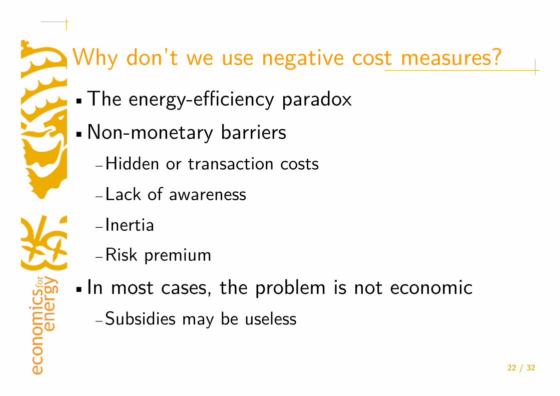
Why don’t we use negative cost measures? • The energy-efficiency paradox • Non-monetary barriers
– Hidden or transaction costs – Lack of awareness – Inertia – Risk premium
• In most cases, the problem is not economic – Subsidies may be useless

23 / 32
Why do some measures look so expensive? • Lack of the right information
– Very difficult to get reliable data (non-ETS) – Data aggregation: there may be niches
• Multiple objectives (e.g. Buildings) – How to allocate the cost?
• Interaction between measures

24 / 32
Low-carbon policies • Carbon price
– Auctioned cap-and-trade
– Safety valve
plus • Technology standards • Technology policies
– Market-pull
– Technology-push
• Education policies • Voluntary approaches

25 / 32
Energy efficiency policies Policy instrument
Low energy prices Taxes; Real time pricing Hidden and transaction costs R&D; Institutional reform
Uncertainty and irreversibility Information programs
Information failures Information programs Bounded rationality Information programs, Education, Standards
Slowness of technological diffusion R&D programs; R&D incentives
Principal-agent problem Information programs; Institutional reform
Capital markets imperfections Financing programs
Divergence with social discount rates Financing programs

26 / 32
Conclusions • We need all options
– Low-carbon energy – Energy efficiency (technology & behavioral changes)
• The potential is huge – But must be estimated correctly
• The cost: – May be very low, even negative – Or very high
• Good policies are required • Adaptation also needs to be factored in

27 / 32
Adaptation to climate change in energy Climate Change
Temperature Rainfall Extreme events
Water
Energy demand Energy supply Energy resource
Glaciers Demand
Efficiency
MiGgaGon
Cooling

28 / 32
Changes in hydro Climate Impacts on Energy Systems 31
rison and WhiĴ ington, 2002; Vicuña et al., 2005).6 The river fl ow series is simulated in hydrological models, which are in turn calibrated to current climate but forced with climate variables (normally from downscaled GCM data), such as precipitation and tem-perature for selected emission scenarios.
The modeling tools for analyzing climate impacts on a hydropower system ulti-mately depend on the complexity of the system, for which two factors can be highlighted (Lucena et al., 2009b). The fi rst is how relevant hydropower generation is for the whole power system, in other words, whether hydroelectricity is complementary to (for ex-ample, the United States and Western Europe) or complemented by (for example, Brazil and Norway) other power sources. If hydroelectricity is complementary to other gener-ating sources, average values for hydropower production generally provide a suĜ cient measure of climate impact. On the other hand, power systems fundamentally based in hydropower must be assessed in terms of a more conservative indicator, such as fi rm power,7 to minimize the risk of power shortages.
The second factor relates to geographical dispersion and the level of integration through transmission capacity. Transmission may play an important role in coping with regional climate variations in interconnected hydropower systems that cover a vast area. In Brazil and Colombia, for example, electricity transmission networks help to optimize the power system’s operation by compensating for regionally diě erent seasonal varia-tions (Lucena et al., 2010b; UPME 2009). In such a case, just as the operation of diě erent
Box 3.1. Projected Changes in Hydropower Generation
Modeling by the Norwegian University of Science and Technology examined climate impacts on river fl ows and hydropower generation to 2050. Systems at highest risk had both a high dependence on hydropower generation for electricity and a declining trend in runoff. South Africa is quoted as one example with a potential reduction of 70 GWh per year in generation by 2050. Afghanistan, Tajikistan, Venezuela, and parts of Brazil face similar challenges.
Source: Hamududu and Killingtveit, 2010.

29 / 32
Water and CO2
Climate Impacts on Energy Systems 43
Most climate change impact assessments focus on water availability. A few studies also include comparisons with projected demand to test the vulnerability of water sup-ply (for example, Arnell, 1999; Dvorak et al., 1997; Joyce et al., 2005; LeĴ enmaier et al.; 1999; Wilby et al., 2006). In general, however, there is limited aĴ ention on the demand side. Changes in land use, higher water demand for crop irrigation, and population shifts caused by climate change are some of the issues that can aě ect the demand for water resources (Frederick and Major, 1997). Multiple uses of water resources (such as human and animal consumption, irrigation, ecosystem maintenance, and fl ood control) add signifi cant complexity to energy modeling. Similarly, it adds a large amount of un-certainty to climate impact assessments on energy systems.
The 2009 Market Report by Lux Research, “Global Energy: Unshackling Carbon From Water,” examined the carbon and water intensity of power production and as-sociated tradeoě s (Figure 3.4). It highlights the challenge of simultaneously reducing GHG emissions and limiting water consumption. Power production from solar PV and wind resources, for example, have the least carbon and water intensity but suf-
Figure 3.4. Effect of Emerging Technologies on Carbon and Water Intensity of Electricity Sources
Source: Lux Research, 2009.

30 / 32
Results: Water availability
0
200
400
600
0
200
400
600
2_Nexus
3_WRWT
01_G
al_C
osta
02_M
ino_
Sil
03_C
antb
r_O
c
04_C
antb
r_O
r
05_D
uero
06_T
ajo
07_G
uadi
ana
08_T
int_
Od_
Pdra
09_G
uada
luqu
ivir
10_G
uad_
Barb
te
11_C
_Med
_And
lz
12_S
egur
a
13_J
ucar
14_E
bro
15_C
ICat
River Basin
Volu
me
hm3
WATER
available
cons

31 / 32
Results: Change in investment
0
5
10
15
Gal
icia
Miñ
o-Si
l
Can
tab_
Oc
Can
tab_
Or
Der
o
Tajo
Gua
dian
a
Tint
o_Pi
edra
Gua
dalu
quiv
ir
Gua
dale
te
Sur
Segu
ra
Juca
r
Ebro
Cat
alun
ya
River Basin
Pow
er (G
W)
SCENARIOUnlimitedStressed

32 / 32
Results: the cost of climate change
0
100
200
300
400
500
600
700
Cos
t (G
igaE
uros
)
SCENARIOUnlimitedStressed
0
100
200
300
400
500
600
700
Cos
t (G
igaE
uros
)
SCENARIOUnlimitedStressed
Planned Cost Real Costs

Thanks for your attention www.upcomillas.es/personal/pedrol


