SIMULATION OF HEATING/COOLING LOAD USING DEST PROGRAM & MEASUREMENT OF HSPF & SEER FOR GEO-SPACE HEATING SYSTEM

L.S Ding1 X.M. Lai2 Y.W. Jian3 R.H. Wang 4 Y.T. Zhang,4 A.Q.Hu5

1College of Environment and Energy Engineering, Beijing University of Technology,

Beijing 100022, China 2Graduate Student, College of Environment and Energy Engineering, BJUT, Beijing 100022, China

3College of Architectural Engineering, BJUT, Beijing 100022, China

4College of Electronic Information & Control Engineering, BJUT, Beijing 100022, China

5Beijing Meteorological Observatory, Beijing 100089, China

ABSTRACT

Using DeST Program, Simulation of Space Heating/cooling Load of two buildings has been conducted for Geo-Space Heating System using Gradient Utilization Techno- logy in university campus. Simulations were conducted in accordance with the different conditions: Temperatures & RH of Rooms, different sources of Weather Data, intensity of persons, Timetable of operation & Equipment, building constructions. Also measurement has been conducted using the measurement system. Then the comparisons between simulation & measurement were made. The range values of (HPF)Sys .h was 3-13, average value was 6-9 based per hour; The values of (HPF)Sys.d & (EER)Sys .d could be obtained through the comparison between measurement & simulation. (HPF)Sys.d values were obtained around 4~7,and (HSPF)Sys was around 5-6 for winter 2005-2006 & 2006-2007. In 2006 summer, consumption of electrical energy was obtained; (EER)Sys.d values based on per day was 2.5~5.3 .In accordance with the analysis of (HPF)Sys .d & (EER)Sys .d, the lower data always appeared in the periods of non-peak & lower load. It tells us where the potential of energy saving will be. The researchers noticed the quite difference between the simulation &

measurement& & try to search the reasons. More efforts & more suggestions will be made for increasing the values of (HSPF)Sys & (SEER) )Sys of the systems.

KEY WORDS

DeST Simulation Measurement HSPF & SEER of Systems Geo-Space Heating

INTRODUCTION

The Demo-Project of Geo-Space Heating in Campus of Beijing University of Technology (BJUT) has been built-up starting with seven years ago under the great support of BJMCDR (Beijing Municipal Committee of Developing & Reforming) & BJMCST (Beijing Municipal Commission of Science & Technology) (Ding, et. al 2006). Three deep wells had been digged in university campus since 2000. Two of them are production wells with depth of 1580m & 1683m respectively. Corresponding flow rate is 70 m3/hr & 84.6 m3/hr. Temperature of geo-water is 52 ℃ . The 3rd well is a re-injection well with depth 1859m. Total geo-water has been re-injected to this well

Proceedings: Building Simulation 2007

- 493 -

after the usage of space heating. Five buildings & a swimming pool have been supplied by the geo-heat in the campus.

SIMULATION OF HEATING/COO- LING LOAD

The Importance of Simulation for Geo- Space Heating & Space Cooling

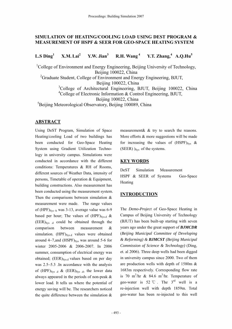
DeST Commercial version has been used to simulate Heating and Cooling Load for building A & B. Which is supplied by the same Geo-water system shown in Fig.1, 2. 3.

Fig.1 Building A

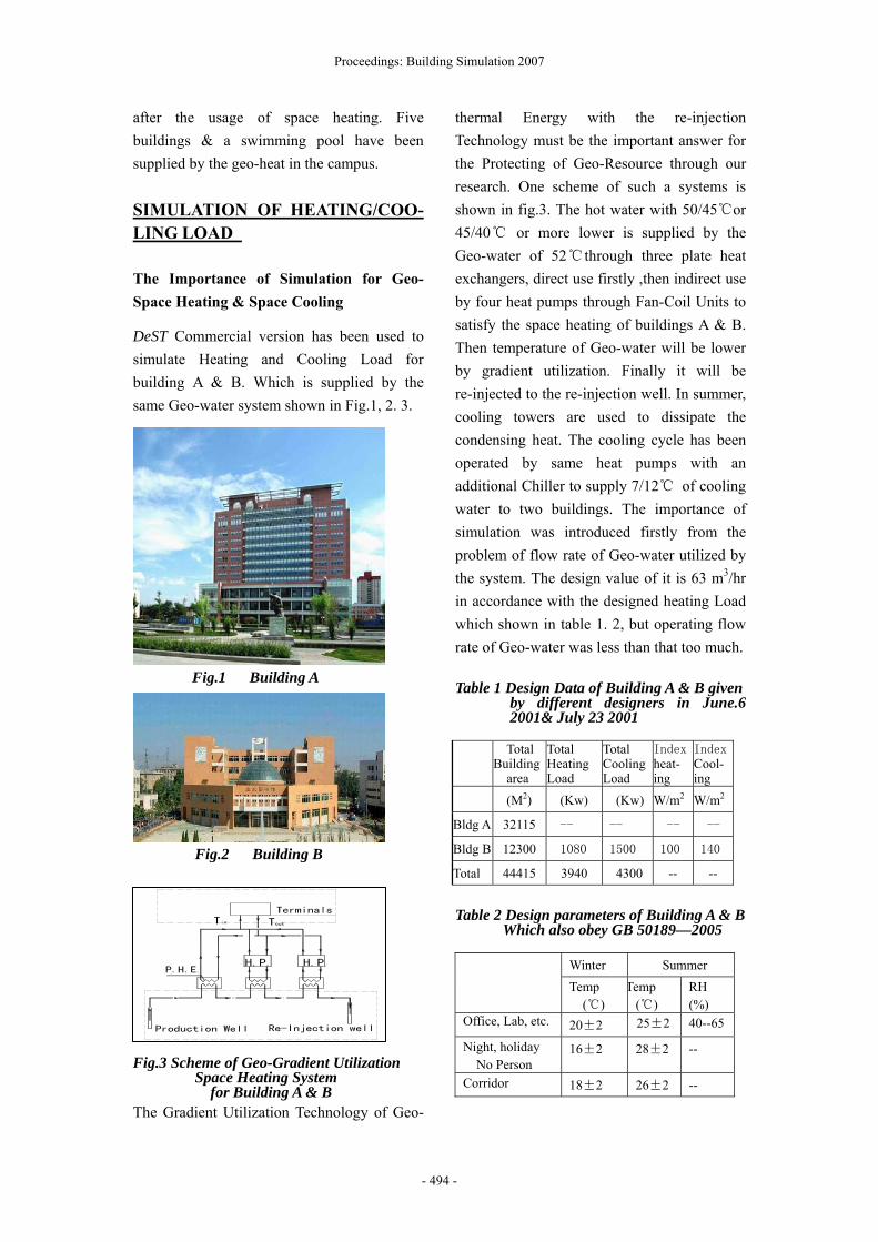
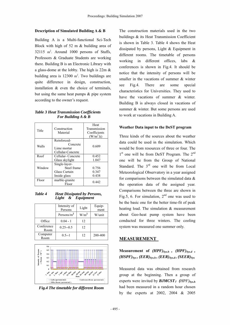
Fig.2 Building B . Fig.3 Scheme of Geo-Gradient Utilization

Space Heating System for Building A & B

The Gradient Utilization Technology of Geo-

thermal Energy with the re-injection Technology must be the important answer for the Protecting of Geo-Resource through our research. One scheme of such a systems is shown in fig.3. The hot water with 50/45℃or 45/40℃ or more lower is supplied by the Geo-water of 52℃through three plate heat exchangers, direct use firstly ,then indirect use by four heat pumps through Fan-Coil Units to satisfy the space heating of buildings A & B. Then temperature of Geo-water will be lower by gradient utilization. Finally it will be re-injected to the re-injection well. In summer, cooling towers are used to dissipate the condensing heat. The cooling cycle has been operated by same heat pumps with an additional Chiller to supply 7/12℃ of cooling water to two buildings. The importance of simulation was introduced firstly from the problem of flow rate of Geo-water utilized by the system. The design value of it is 63 m3/hr in accordance with the designed heating Load which shown in table 1. 2, but operating flow rate of Geo-water was less than that too much. Table 1 Design Data of Building A & B given

by different designers in June.6 2001& July 23 2001

Total

Buildingarea

Total Heating Load

Total Cooling

Index heat-

Load ing

Index Cool- ing

(M2) (Kw) (Kw) W/m2 W/m2

Bldg A 32115 -- -- -- --

Bldg B 12300 1080 1500 100 140

Total 44415 3940 4300 -- --

Table 2 Design parameters of Building A & B

Which also obey GB 50189—2005

Winter Summer

Temp (℃)

Temp (℃)

RH (%)

Office, Lab, etc. 20±2 25±2 40--65

Night, holiday No Person

16±2 28±2 --

Corridor 18±2 26±2 --

Proceedings: Building Simulation 2007

- 494 -

Description of Simulated Building A & B

Building A is a Multi-functional Sci-Tech Block with high of 52 m & building area of 32115 m2. Around 1000 persons of Staffs, Professors & Graduate Students are working there. Building B is an Electronic Library with a glass-dome at the lobby. The high is 22m & building area is 12300 m2. Two buildings are quite difference in design, construction, installation & even the choice of terminals, but using the same heat pumps & pipe system according to the owner’s request. Table 3 Heat Transmission Coefficients

For Building A & B

Title Construction Material

Heat Transmission Coefficients

(W/m2.k)

Walls

Reinforced- Concrete

Lime mortar Cellular-Concrete

0.609

Roof Cellular- Concrete Glass skylight

0.452 1.047

Window

Single-layer- Steel frame

Glass Curtain Inside glass

0.756 0.347 0.438

Floor marble-granite Floor 0.442

Table 4 Heat Dissipated by Persons,

Light & Equipment

Intensity of Persons Light Equip-

ment Persons/m2 W/m2 W/unit

Office 0.04 - 1 12 Conference

Room 0.25--0.5 12

Computer Room

0.5--1 12 200-400

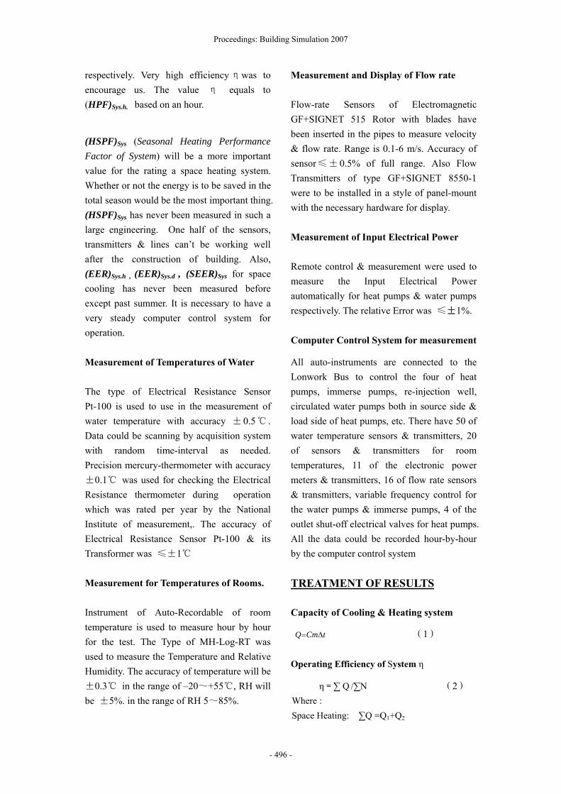
Fig.4 The timetable for different Room

The construction materials used in the two buildings & its Heat Transmission Coefficient is shown in Table 3. Table 4 shows the Heat dissipated by persons, Light & Equipment in different rooms. The timetable of persons working in different offices, labs & conferences is shown in Fig.4. It should be notice that the intensity of persons will be smaller in the vacations of summer & winter see Fig.4. There are some special characteristics for Universities. They used to have the vacations of summer & winter. Building B is always closed in vacations of summer & winter. But some persons are used to work at vacations in Building A.

Weather Data input to the DeST program

Three kinds of the sources about the weather data could be used in the simulation. Which would be from resources of three or four. The 1st one will be from DeST Program. The 2nd one will be from the Group of National Standard. The 3rd one will be from Local Meteorological Observatory in a year assigned for comparisons between the simulated data & the operation data of the assigned year. Comparisons between the three are shown in Fig.5, 6. For simulation, 2nd one was used to be the basic one for the better time-fit of peak heating load. The simulation & measurement about Geo-heat pump system have been conducted for three winters. The cooling system was measured one summer only.

MEASUREMENT

0

0.1

0.2

0.3

0.4

0.5

0.6

1 Ja

n.

31 J

an.

2 M

ar.

1 Apr.

1-May

31-M

ay

30-Ju

n30

-Jul

29-A

ug

28-Sep

28-O

ct

27-N

ov

27-D

ec

Date

Inte

nsity

of

Pers

ons

( P

erso

n /

M 2

)

Labs (persons/m2) Conference.Rrom (persons/m2)Office Room ( persons/m2 )

Measurement of (HPF)Sys.h , (HPF)Sys.d , (HSPF)Sys , (EER)Sys.h , (EER)Sys.d , (SEER)Sys

Measured data was obtained from research group at the beginning. Then a group of experts were invited by BJMCST；(HPF)Sys.h had been measured in a random hour chosen by the experts at 2002, 2004 & 2005

Proceedings: Building Simulation 2007

- 495 -

respectively. Very high efficiencyηwas to encourage us. The value η equals to (HPF)Sys.h. based on an hour.

(HSPF)Sys (Seasonal Heating Performance Factor of System) will be a more important value for the rating a space heating system. Whether or not the energy is to be saved in the total season would be the most important thing. (HSPF)Sys has never been measured in such a large engineering. One half of the sensors, transmitters & lines can’t be working well after the construction of building. Also, (EER)Sys.h , (EER)Sys.d , (SEER)Sys for space cooling has never been measured before except past summer. It is necessary to have a very steady computer control system for operation. Measurement of Temperatures of Water The type of Electrical Resistance Sensor Pt-100 is used to use in the measurement of water temperature with accuracy ±0.5℃ . Data could be scanning by acquisition system with random time-interval as needed. Precision mercury-thermometer with accuracy ±0.1℃ was used for checking the Electrical Resistance thermometer during operation which was rated per year by the National Institute of measurement,. The accuracy of Electrical Resistance Sensor Pt-100 & its Transformer was ≤±1℃ Measurement for Temperatures of Rooms. Instrument of Auto-Recordable of room temperature is used to measure hour by hour for the test. The Type of MH-Log-RT was used to measure the Temperature and Relative Humidity. The accuracy of temperature will be ±0.3℃ in the range of –20～+55℃, RH will be ±5%. in the range of RH 5～85%.

Measurement and Display of Flow rate Flow-rate Sensors of Electromagnetic GF+SIGNET 515 Rotor with blades have been inserted in the pipes to measure velocity & flow rate. Range is 0.1-6 m/s. Accuracy of sensor≤±0.5% of full range. Also Flow Transmitters of type GF+SIGNET 8550-1 were to be installed in a style of panel-mount with the necessary hardware for display. Measurement of Input Electrical Power Remote control & measurement were used to measure the Input Electrical Power automatically for heat pumps & water pumps respectively. The relative Error was ≤±1%.

Computer Control System for measurement

All auto-instruments are connected to the Lonwork Bus to control the four of heat pumps, immerse pumps, re-injection well, circulated water pumps both in source side & load side of heat pumps, etc. There have 50 of water temperature sensors & transmitters, 20 of sensors & transmitters for room temperatures, 11 of the electronic power meters & transmitters, 16 of flow rate sensors & transmitters, variable frequency control for the water pumps & immerse pumps, 4 of the outlet shut-off electrical valves for heat pumps. All the data could be recorded hour-by-hour by the computer control system

TREATMENT OF RESULTS

Capacity of Cooling & Heating system

Q Cm t= Δ （1）

Operating Efficiency of System η

η＝∑ Q /∑N （2）

Where : Space Heating: ∑Q =Q +Q1 2

Proceedings: Building Simulation 2007

- 496 -

∑N＝N +N +N1 2 3

Space Cooling : ∑Q =Q +Q3 4

∑N=N +N +N +N +N +N +N4 5 6 7 8 9 10

Heating Performance Factor of System per Day（HPF）Sys.d

24

124

1

ys.( ) id

ii

QHPF s

E

=

=

=∑

∑

i

（3）

Heating Seasonal Performance Factor of System (HSPF)Sys

1

1

( )( )

( )

N

j jjN

j jj

sysQ T h

HSPFE T h

=

=

=∑

∑ （4）

Seasonal Energy Efficiency Ratio of System for Cooling (SEER)Sys

1

1

sys( )

(SEER)( )

N

k kk

N

k kk

Q T h

E T h

=

=

=∑

∑

k

(5)

RESULTS & COMPARISONS

Simulated Space Heating / Cooling Load vs. standard Building Conditions

The result using DesT program is shown in Fig.7. Which was based on the standard conditions: heat transmission coefficients, dissipated heat of persons, lights, equipment, work-timetable & the fresh air volume were obtained from Table 3、4; Fig.7 shows the standard simulated conditions for heating & cooling load of building (A+B). The choice of our simulated temperatures of main rooms are 20℃ in winter & 26℃ with RH 60% in summer. Temperatures of other rooms are

assigned in Table 2. Different temperature of rooms for load simulation were chosen for comparisons, for instance, 22 ℃ ,23 ℃ in winter; 25℃, 100%,90% RH in summer.

Comparisons of Heating Load between the Simulation & Measurement

Fig.8 shows the measured temperature of rooms for Building A. Temperature range at office hours was around 22-24℃except the period of winter vacation. Fig.9, 10 shows the heating load hr-by-hr from the measured & the simulated separately. Fig.11 shows the comparison between the measured & the simulated data. It should be noticed that the measured data were larger than that of the simulated data in the zone of basic load & minimum load where the high temperatures of rooms in happened for building A. People of Building A always open their windows for dissipating the surplus heat at that period in accordance with investigation while the temperature of room for Building B can’t reach to such a higher range. Fig.12, 13 & 14 shows the comparisons of heating load between simulated & measured data in different conditions shown in table 5

Table 5 Different Conditions for Comparison

Rm. Temp. (℃)

Conditions Bldg. A

Bldg. B

Vaca- tion

Weath-er data

Simu. 20 20 No Std. Fig.12 Meas. 23 18 Yes 2006

winterSimu. 20 20 No Std.

Fig.13 Simu 22 18 Yes 2006

winterSimu. 22 18 Yes 2006

winter Fig.14 Meas. 23 18 Yes 2006

winter Fig.12 shows the larger difference between the standard simulated data under the historical weather data & measured data under the same year weather data. Fig.13 shows the medium

Proceedings: Building Simulation 2007

- 497 -

difference between simulated heating load (Trm=20/20℃ without vacation) & another simulated heating load (Trm=22/18℃ with winter vacation & 2006—2007 winter weather data). Fig.14 shows the smaller difference between the simulated heating load (Trm=22/18 ℃ with winter vacation) & measured heating load (Trm=23/18℃ have winter vacation & 2006—2007 winter weather data.). It shows the importance of conditions for comparisons. Comparison of Average Daily Heating Load Between designed, simulated & measured It is shown in Fig.15. In accordance with the National Standard the designed heating load is defined as the 2nd larger average daily heating load. The simulated data for building (A+B) should be around 2150 kW which is smaller than the given design heating load 3940 kW and is equals to 54.8% of it. The reasons must be in the following order: Warm winter first, Increasing of persons & computers or other equipment in the building, Decreasing of Peak-Load for the vacation of summer & winter, Over-design for safety. At the same time, Cooling Load must be increased.

Comparison of the Flow-rate of Geo-water Between the Measured data vs. Designed

It is shown in Fig.16 for winter 2006-2007. The actual flow rate of geo-water measured is around 10-24 m3/hr in winter 2006-2007 while around 23-27 m3/hr in winter 2005-2006 which is much more lower than that of the designed data 63 m3/hr which implied the over-design of heating load.

Comparison of Cooling Load Between the Simulated vs. Measured

It is shown in Fig. 17 & 18. The simulation conditions : T=26℃& RH=60%. Measured conditions : T=25.04℃ & RH=73.9% for building A; T=27℃& RH=80% for building B which could be found in Fig.21. It shows a

steady temperature & relative high RH≈80% for an office of building B while the outside was rainy days with RH (%) ≈ 100%. Fig.19 & 20 show the supplied temperature of cooling water generally it keeps 10-12℃, the minimum was 7-8℃ It should be noticed that measured data is smaller than the simulated data in most of the period of the summer. The reasons must be from the temperature of cooling water. It is not low enough so that the cooling capacity of de-humidity is not good enough. This is always happened in an over-designed system & over-sized water pumps. It causes the difficulty in regulations.

The Results & Analysis of (HPF)Sys.d , (HSPF) Sys.h , (HSPF) Sys. & (SEER) Sys.

Fig.23 shows the measured average daily (HPF)sys.d based on per day for building (A+B) in winter 2006— 2007. The high of (HPF)sys.d

was reached to 10.94 ,the low till 3.7. The average (HPF)sys.d will be around 4-7. Trend line had been shown that low value was happened in the zone of low heating load. Fig.24 shows measured value of (HPF)SYS.h

based on an hour at 9:00am—10:00am every morning during the winter 2006—2007. As we know that the heat pump always starts-up at the morning to satisfy the higher starting load. The efficiency always keeps a higher value while the heat pump was operated in a full-load condition. The high of (HPF)SYS.h

was reached to 13.0 ,the low till 3.2. The average (HPF) SYS.h will be around 6-9. Trend line also shows the same range. The value of (HSPF)SYS will be around 5-6 for the 2005 & 2006 winter. Fig.22 shows the comparison of (EER) SYS d

based on day between the simulated & measured in summer 2006. The simulated data was larger than that of the measured data because of the absence of the latent cooling load in the operating. The value of (SEER) SYS will be lower than that of the winter. Although

Proceedings: Building Simulation 2007

- 498 -

the consumption of simulated & measured seasonal cooling load & the consumption of Input power were obtained, but the measured latent cooling load is too small. It caused the relative humidity of rooms was pretty high. Building B was closed in the total summer vacation, but the water pump was operating. So the simulated cooling load was much more larger than that of the measured data. The potential of increasing (SEER) SYS will be clear. Continuing this work in coming summer & winter will be necessary. Economic analysis is shown in Table 6.

CONCLUSIONS

The correctness of simulation has to prove by the measurement. The reasonable reasons must be able to find from the difference between two sides.

DeST is one of the most important programs in Building Simulation field. It will be an important basis in research.

Great Importance of Comparison Between Simulation & Measurement has already been proved. The steady & correctness of Auto-instruments will be more important.

(HSPF)SYS & (SEER)SYS for an Air- Conditioning System will be more important. Only the equipment has the Rating Standard until now. So the Simulation & measurement will be more useful for rating a system.

Design engineers should be designing the engineering in accordance with the requirement of operation & regulation.

Most of the operation time will be in the period of non-peak load. The more consideration about it will be, the more energy

saving will be.

ACKNOWLEDGEMENTS

The authors will be in acknowledgements of the help from Academician Jiang, Yi & Dr. Jian, Yiwen for spending their time to check out the correctness of our campus building simulation using DeST program, also the help from Dr. Yan, da for helping us to result the problems in using DeST. It is appreciate to graduate students L.F. Liu, C.J. Song, H.M. Zhu & workers.

REFERENCES

Jiang, Yi, Yan, Da, et al, “ DesT Commercial Version”, 2004, Tsinghua University, Beijing, China

Ding, L.S, Zhang, C.C. et al. 2006, “Seven Years Review On the Demo-Project of Geo-Space Heating in the Campus of Beijing University of Technology”, Journal of HV&AC, Vol.36 additional Edition, P.199-207.

Ding, L.S, Zhang, C.C. et al. 2004, “From Deep Aquifer to Shallow Aquifer & Ground Source to Consider the Energy Source Construction for the 2008 Olympic GYMs ”,Machinery Engineering & Design ,Vol.4,2004.

Ding, L.S, Zhang, C.C. Yin, F.G. et al. 2002 . “Energy Saving of Water Source Heat Pump System Using Aquifer Geothermal Hot Water to be Auxiliary Heat Source ”, Proceedings of Heat Pump Conference , Beijing 2002.

Yu, Fengju, Yin, Fugeng et al. 2002, “ System Schemes & Peak Load Treatment on the Gradient Utilization Technology of Low Temperature Geothermal Energy for Space heating” Proceedings of HV & AC Conference.,p.211-214.

GB 50189-2005 “Design Standard for energy efficiency of public building”, P. R. China

Proceedings: Building Simulation 2007

- 499 -

Adnot,A. et al. “Energy Efficiency & Certification of Central Air-Conditioners” Final Reports Vol.1 ,2 ,3 April 2003

NOMENCLATURE

η——Total Energy Efficiency Ratio in the System of Geo-Space Heating kw/kw ；

C——Specific Heat of Water ,4.181kJ/kg .oC；

EER---- Energy Effective Ratio for Chiller Unit;

(EER)sys.d-----Average Energy Effective Ratio per day for a Chiller Unit system

(EER)sys.h ----- Average Energy Effective Ratio per hour for a Chiller Unit system

( )jE T —Input Power for Load Zones j（Kwe）；

( )kE T —Input Power for Load Zones k（Kwe）；

24

1i

iE

=∑ —Electrical Energy Consumption per day.

kw;

jh ——hours values for Load Zones j（hr）；

kh ——hours values for Load Zones k（hr）；

(HPF)sys.dAverage Heating Performance Factor of System per day for heat pump system

(HPF)sys.h——Average Heating Performance Factor of System per hour for heat pump system

(HSPF)sys——Heating Seasonal Performance Factor of System for heat pump system

(HSPF) ——Heating Seasonal Performance Factor of System for Heat Pump Unit

m —— mass flow rate of fluid, kg/s ∑N——Input Power for space Geo-Heating

/Cooling system, kw；

N1——Input Power for a heat pump equipment，kW；

N2——Input Power of water pump immersed in Geothermal well ，kw ；

N3——Input Power of Cycled water pump in Source Side of Heat Pump，kw ；

N4——Input Power of Heat Pump, kw ； N5——Input Power of Chillers, kw ； N6——Input Power of Cycled Water Pump in

Load Side of Heat Pump, kw ； N7——Input Power of Cooling Tower, kw ； N8——Input Power of Cycled Water Pump for

Cooling Tower, kw ； N9——Input Power of Fan-Coil Unit，kw ； N10——Input Power of Fresh Air Unit，kW； Q——-Total Capacity of Cooling/Heating supplied by a system，kW； Q1——Heating Capacity of 1st stage of Geo-

Heating System , kW； Q2——Heating Capacity of Heat Pump ,kW； Q3——Cooling Capacity of Chiller ,kW； Q4——Cooling Capacity of Heat Pump ,kW； Qi—— Space Load Hour by Hour per day, kW；

( )jQ T --Heating Capacity of Load Zone j under Outside temperature Tj，（KWt）；

( )kQ T —Heating Capacity of Load Zone k under Outside temperature Tk，（KWt）；

∑Q——-Total Capacities for a Geothermal Heating/Cooling System , kW；

(SEER)—Seasonal Energy Effective Ratio for a Chiller Unit

(SEER)sys—Seasonal Energy Effective Ratio for an air conditional system using Chiller.

jT ——Average Outside Temperature in Load

Zone j；

kT ——Average Outside Temperature in Load

Zone k；

tΔ — Temperature Difference between Supply

/Return Water to a system oC；

24

1i=∑ ——Accumulative Total through a day;

1j=

N

∑ — Accumulative Total through the Total

Heating Season；

1

N

k=∑ —Accumulative Total through the Total

Cooling Season;

Proceedings: Building Simulation 2007

- 500 -