57
The Sixth Superstring Bachelor thesis in Physics Author: Pelle Werkman Supervisor: Diederik Roest June 10 2013
The Sixth Superstring
Bachelor thesis in Physics
Author: Pelle WerkmanSupervisor: Diederik RoestJune 10 2013
Abstract
The objective of this thesis is to discuss the possible new superstring proposed by Savdeep Sethi in April 2013. Inorder to do this, we give an introduction to string theory pretty much from the ground up - starting with the 26dimensional bosonic string and then on to the five different flavours of ten dimensional superstring. Along the waywe will discuss some of the dualities and transformations that relate these strings to each other. Savdeep Sethi’ssuperstring will arise from just such a transformation: an orientifold of the type IIB superstring. Eventually we willstart to hone in on the modern picture of string theory, which is that the superstrings are all perturbative limits ofan 11-dimensional theory called ’M-theory’. We will discuss how Savdeep Sethi’s superstring may fit into this webof theories. By construction, the new string looks very similar to the Type I superstring. We will have to find away to distinguish the two from each other. By comparing the Kaluza-Klein towers that result from their M-theorydescriptions, we will find a sharp distinction between Type I and the new superstring. However, we will be left withquestions about the consistency of the new string and about its place in the M-theory web.

Contents
1 Introduction 3
2 The bosonic string 62.1 Constructing the action . . . . . . . . . . . . . . . . . . . . . . . . . . . . . . . . . . . . . . . . . . . . 6
2.1.1 The point particle action . . . . . . . . . . . . . . . . . . . . . . . . . . . . . . . . . . . . . . . 62.1.2 The string action . . . . . . . . . . . . . . . . . . . . . . . . . . . . . . . . . . . . . . . . . . . . 62.1.3 Choosing a parametrization . . . . . . . . . . . . . . . . . . . . . . . . . . . . . . . . . . . . . . 72.1.4 The Polyakov action . . . . . . . . . . . . . . . . . . . . . . . . . . . . . . . . . . . . . . . . . . 8
2.2 Symmetries of the Polyakov action and the conformal gauge . . . . . . . . . . . . . . . . . . . . . . . . 82.2.1 Poincare transformations . . . . . . . . . . . . . . . . . . . . . . . . . . . . . . . . . . . . . . . 82.2.2 Reparametrization . . . . . . . . . . . . . . . . . . . . . . . . . . . . . . . . . . . . . . . . . . . 82.2.3 Weyl rescaling . . . . . . . . . . . . . . . . . . . . . . . . . . . . . . . . . . . . . . . . . . . . . 92.2.4 Gauge fixing and residual symmetry: the light cone gauge . . . . . . . . . . . . . . . . . . . . . 9
2.3 Boundary conditions: open and closed strings . . . . . . . . . . . . . . . . . . . . . . . . . . . . . . . . 102.4 Mode expansion . . . . . . . . . . . . . . . . . . . . . . . . . . . . . . . . . . . . . . . . . . . . . . . . 10
2.4.1 The closed string . . . . . . . . . . . . . . . . . . . . . . . . . . . . . . . . . . . . . . . . . . . . 112.4.2 Virasoro constraints . . . . . . . . . . . . . . . . . . . . . . . . . . . . . . . . . . . . . . . . . . 112.4.3 The open string . . . . . . . . . . . . . . . . . . . . . . . . . . . . . . . . . . . . . . . . . . . . . 12
2.5 Quantization . . . . . . . . . . . . . . . . . . . . . . . . . . . . . . . . . . . . . . . . . . . . . . . . . . 122.5.1 Covariant quantization . . . . . . . . . . . . . . . . . . . . . . . . . . . . . . . . . . . . . . . . . 122.5.2 Dealing with the ghosts . . . . . . . . . . . . . . . . . . . . . . . . . . . . . . . . . . . . . . . . 132.5.3 The mass operators . . . . . . . . . . . . . . . . . . . . . . . . . . . . . . . . . . . . . . . . . . 132.5.4 Light-cone gauge quantization . . . . . . . . . . . . . . . . . . . . . . . . . . . . . . . . . . . . . 14
2.6 The spectrum . . . . . . . . . . . . . . . . . . . . . . . . . . . . . . . . . . . . . . . . . . . . . . . . . . 152.6.1 The open string . . . . . . . . . . . . . . . . . . . . . . . . . . . . . . . . . . . . . . . . . . . . . 152.6.2 The closed string . . . . . . . . . . . . . . . . . . . . . . . . . . . . . . . . . . . . . . . . . . . . 15
3 The supersymmetric string 173.1 The RNS formalism . . . . . . . . . . . . . . . . . . . . . . . . . . . . . . . . . . . . . . . . . . . . . . 17
3.1.1 The action and equations of motion . . . . . . . . . . . . . . . . . . . . . . . . . . . . . . . . . 173.1.2 World-sheet supersymmetry . . . . . . . . . . . . . . . . . . . . . . . . . . . . . . . . . . . . . . 183.1.3 The super-Virasoro constraints . . . . . . . . . . . . . . . . . . . . . . . . . . . . . . . . . . . . 183.1.4 Mode expansion . . . . . . . . . . . . . . . . . . . . . . . . . . . . . . . . . . . . . . . . . . . . 193.1.5 Covariant quantization . . . . . . . . . . . . . . . . . . . . . . . . . . . . . . . . . . . . . . . . . 203.1.6 Light-cone gauge quantization . . . . . . . . . . . . . . . . . . . . . . . . . . . . . . . . . . . . . 223.1.7 GSO projection . . . . . . . . . . . . . . . . . . . . . . . . . . . . . . . . . . . . . . . . . . . . . 243.1.8 Closed string spectrum . . . . . . . . . . . . . . . . . . . . . . . . . . . . . . . . . . . . . . . . . 24
3.2 The GS formalism . . . . . . . . . . . . . . . . . . . . . . . . . . . . . . . . . . . . . . . . . . . . . . . 253.2.1 Point particle action . . . . . . . . . . . . . . . . . . . . . . . . . . . . . . . . . . . . . . . . . . 263.2.2 Superstring action . . . . . . . . . . . . . . . . . . . . . . . . . . . . . . . . . . . . . . . . . . . 263.2.3 Quantization . . . . . . . . . . . . . . . . . . . . . . . . . . . . . . . . . . . . . . . . . . . . . . 273.2.4 The massless spectrum . . . . . . . . . . . . . . . . . . . . . . . . . . . . . . . . . . . . . . . . . 28
3.3 A look at supergravity . . . . . . . . . . . . . . . . . . . . . . . . . . . . . . . . . . . . . . . . . . . . . 293.3.1 11-dimensional supergravity . . . . . . . . . . . . . . . . . . . . . . . . . . . . . . . . . . . . . . 293.3.2 Type IIB supergravity . . . . . . . . . . . . . . . . . . . . . . . . . . . . . . . . . . . . . . . . . 30
3.4 Perturbative symmetries of Type IIB . . . . . . . . . . . . . . . . . . . . . . . . . . . . . . . . . . . . . 313.5 Anomaly cancellation . . . . . . . . . . . . . . . . . . . . . . . . . . . . . . . . . . . . . . . . . . . . . 32
1
3.6 The heterotic strings . . . . . . . . . . . . . . . . . . . . . . . . . . . . . . . . . . . . . . . . . . . . . . 323.7 The web of dualities . . . . . . . . . . . . . . . . . . . . . . . . . . . . . . . . . . . . . . . . . . . . . . 32
4 Compactification 334.1 T-duality and D-branes in the bosonic theory . . . . . . . . . . . . . . . . . . . . . . . . . . . . . . . . 33
4.1.1 Closed strings . . . . . . . . . . . . . . . . . . . . . . . . . . . . . . . . . . . . . . . . . . . . . . 334.1.2 Open strings . . . . . . . . . . . . . . . . . . . . . . . . . . . . . . . . . . . . . . . . . . . . . . 354.1.3 D-branes and gauge fields . . . . . . . . . . . . . . . . . . . . . . . . . . . . . . . . . . . . . . . 364.1.4 Wilson lines . . . . . . . . . . . . . . . . . . . . . . . . . . . . . . . . . . . . . . . . . . . . . . . 364.1.5 String charge . . . . . . . . . . . . . . . . . . . . . . . . . . . . . . . . . . . . . . . . . . . . . . 39
4.2 T-duality and D-branes in superstring theory . . . . . . . . . . . . . . . . . . . . . . . . . . . . . . . . 394.2.1 D-brane charges . . . . . . . . . . . . . . . . . . . . . . . . . . . . . . . . . . . . . . . . . . . . 394.2.2 Stability of D-branes . . . . . . . . . . . . . . . . . . . . . . . . . . . . . . . . . . . . . . . . . . 404.2.3 Type II T-duality . . . . . . . . . . . . . . . . . . . . . . . . . . . . . . . . . . . . . . . . . . . 41
4.3 Kaluza-Klein towers and 11-dimensional supergravity . . . . . . . . . . . . . . . . . . . . . . . . . . . . 424.3.1 A note on BPS states . . . . . . . . . . . . . . . . . . . . . . . . . . . . . . . . . . . . . . . . . 424.3.2 M-theory - Type II duality . . . . . . . . . . . . . . . . . . . . . . . . . . . . . . . . . . . . . . 42
4.4 The web of dualities: part II . . . . . . . . . . . . . . . . . . . . . . . . . . . . . . . . . . . . . . . . . 44
5 Orbifolds and Orientifolds 455.1 General features of orbifolds . . . . . . . . . . . . . . . . . . . . . . . . . . . . . . . . . . . . . . . . . . 455.2 Type IIA as an orbifold . . . . . . . . . . . . . . . . . . . . . . . . . . . . . . . . . . . . . . . . . . . . 455.3 General features of orientifolds . . . . . . . . . . . . . . . . . . . . . . . . . . . . . . . . . . . . . . . . 465.4 Type I as an orientifold . . . . . . . . . . . . . . . . . . . . . . . . . . . . . . . . . . . . . . . . . . . . 46
5.4.1 Type I’ . . . . . . . . . . . . . . . . . . . . . . . . . . . . . . . . . . . . . . . . . . . . . . . . . 475.5 Heterotic-Type I S-duality . . . . . . . . . . . . . . . . . . . . . . . . . . . . . . . . . . . . . . . . . . . 475.6 The web of dualities: part III . . . . . . . . . . . . . . . . . . . . . . . . . . . . . . . . . . . . . . . . . 48
6 Savdeep Sethi’s Superstring 496.1 A different orientifold . . . . . . . . . . . . . . . . . . . . . . . . . . . . . . . . . . . . . . . . . . . . . 496.2 M-theory BPS spectrum . . . . . . . . . . . . . . . . . . . . . . . . . . . . . . . . . . . . . . . . . . . . 496.3 The strong coupling limit . . . . . . . . . . . . . . . . . . . . . . . . . . . . . . . . . . . . . . . . . . . 51
Conclusion 52
Appendices 53
A Review of spinors 53A.1 Gamma matrices in d dimensions . . . . . . . . . . . . . . . . . . . . . . . . . . . . . . . . . . . . . . . 53A.2 Spinors of SO(1, d− 1) . . . . . . . . . . . . . . . . . . . . . . . . . . . . . . . . . . . . . . . . . . . . . 53A.3 Spin transformations . . . . . . . . . . . . . . . . . . . . . . . . . . . . . . . . . . . . . . . . . . . . . . 54A.4 Fierz identity . . . . . . . . . . . . . . . . . . . . . . . . . . . . . . . . . . . . . . . . . . . . . . . . . . 55
Chapter 1
Introduction
What is string theory?
String theory is a theory of nature where the fundamental building blocks are one-dimensional objects called strings.It was first developed in the 1960s as an attempt to describe the strong nuclear force. In this respect, it waseventually superseded by quantum chromodynamics. In the mid-1970s it was realized that string theory coulddescribe a consistent quantum gravity theory. Since then, string theory has been a candidate for a grand unifiedtheory, poised to bring all of the forces of nature together in a single theoretical framework. From this perspective,the big claim of string theory is that the fundamental particles in the standard model are nothing more than thevibrational modes of quantum strings.
Just why exactly is string theory necessary to provide a quantum theory of gravity? This can be seen in severalways. In ordinary quantum field theory, one requires that two fields at space-like separation should (anti)commute2.However, when the field in question is the spacetime metric itself, as would be the case in quantum gravity, it isnot clear in advance whether two points have space-like separation at all! Secondly, the metric suffers quantumfluctuations, just like any other field. These difficulties make sure that straightforward attempts to build a quantumgravity theory all suffer from uncontrollable infinities. More precisely, they are not renormalizable. String theorygets around these difficulties because it has a built-in length scale, the string length `s, which makes it, in some sense,insensitive to the irregularities of spacetime at the smallest scale. This is actually a principle that string theory hasin common with all modern quantum gravity theories.
The length scale `s is actually the only dimensionful adjustable parameter in string theory1, whereas the standardmodel has 19.1 This is due to string theory’s highly restricted nature. For example, in string theory the dimensionalityof spacetime is determined by a calculation, instead of a measurement. The bosonic string lives in 26 dimensions,whereas the superstring lives in 10 dimensions. The fact that strings are only consistent in dimensions higher thanthe 4 we actually observe needs to be accounted for. One solution is that all but 4 of the spacetime dimensions arecompactified: they close in on themselves like a circle.
Roughly speaking, there are two different kinds of string theories: bosonic string theory and superstring theory.The bosonic string has mostly been abandoned as a convincing theory of nature, because it does not incorporatefermions. The new string that we intend to examine is a superstring. There are, as-of-yet, five known flavors ofsuperstring. In the 1990s it was realized that these were related by a large number of dualities. The picture thatemerged was that the superstrings are all perturbative limit of a more fundamental theory called ’M-theory’, whichlives in 11 dimensions, and has a low-energy limit called 11-dimensional supergravity. We can summarize with apicture of the so-called web of dualities (taken from Becker, Becker, Schwarz2):
1This is the only parameter in its formulation. There still is a huge landscape of possible solutions.
3

We will revisit this picture a number of times throughout the rest of the thesis, each time updating it with ournew knowledge. The proposed new superstring would represent a seventh spoke on this web.
Let’s outline the structure of the rest of the thesis:
Bosonic strings
We will start by examining the relatively simple bosonic string. This will be useful to gain some familiarity withstring theory concepts. Savdeep Sethi’s string is not a bosonic string. When we construct the spectrum, we willencounter some familiar particles, and we will immediately see string theory’s big claim being actualized to someextent. However, the bosonic string can’t provide a full theory of nature by itself, since its spectrum does not containfermions. To make the bosonic string theory abide by Lorentz invariance, the dimensionality of spacetime will berestricted to D = 26. The bosonic string does not seem to have a place by itself in the M-theory web, but it entersinto the description of the heterotic superstrings E8 × E8 and O(32). We discuss the bosonic string in Chapter 2.
Superstrings
The strings that may actually provide us with a convincing theory of nature (they do include fermions, for instance)are all supersymmetric strings, or superstrings. That means that there is a symmetry transformation relating thefermions and the bosons to each other. Every boson is given its own supersymmetric partner. We will construct thesuperstring in much the same way we did the bosonic string. Only this time we will make things considerably moreabstract by introducing anti-commuting Grassman coordinates.
The supersymmetric string comes in (as-of-yet) five different flavours. Savdeep Sethi’s proposed string is apotential sixth flavour. We discuss the type IIB, IIa and type I superstrings in Chapter 3. A number of consistencychecks restricts the dimension of spacetime in these theories to D = 10, in apparent conflict with the bosonic string.
Compactification
Superstrings live in ten dimensions. In order to make this consistent with reality, all but 4 of these dimensions haveto be compactified. We discuss compactification in Chapter 4.
Symmetries and dualities, orbifolds and orientifolds
When we discuss the bosonic and supersymmetric strings, we will discuss a number of transformations that relatethe different string theories to each other. For example, we will see that the Type IIA string can be obtainedfrom the Type IIB string by an orbifold projection. We will also discuss so-called duality symmetries, which aretransformations that identify two theories that at first glance seem to be completely different. T-duality, which relatestheories on large compactified dimensions to theories on small compactified dimensions, will feature prominently inChapter 4. We discuss orbifolds and orientifolds in Chapter 5.

The new superstring
Once this is done we will be sufficiently equipped to understand Savdeep Sethi’s proposition of a new superstring.We will examine whether or not the proposition really leads to a new, inequivalent superstring. In particular, thereis doubt over whether the new string is equivalent to the Type I superstring, because they are formulated in a verysimilar way. The last chapter of the thesis is devoted to discussing the new superstring.

Chapter 2
The bosonic string
In this chapter we will mostly follow the development of the bosonic string as described in Becker Becker Schwarz2,interjected with information from Zwiebach1 and Tong3.
2.1 Constructing the action
2.1.1 The point particle action
We know that free point particles travel along geodesics, which are the paths of minimum proper length. This allowsus to easily construct the following action:
S0 = −α∫ds (2.1)
In our system of units ~ = c = 1, so we see that the constant α has units of inverse length, which is equivalent tounits of mass. We therefore choose to identify this constant with the mass of the point particle. We can easily seethat this leads to the correct equations of motion in the non-relativistic limit.
We may parametrize the path of the point particle (its world line) with Xµ = Xµ(τ). Our action becomes:
S0 = −m∫ √
−gµν(X)XµXνdτ (2.2)
Here gµν(X) is the background metric. An application of the chain rule shows that this action is reparametrizationinvariant. This will be of great use to us in the future, as it will allow us to choose convenient gauges to work in.
2.1.2 The string action
Just as the zero-dimensional point particle traces out a one-dimensional world line on a spacetime diagram, a one-dimensional string traces out a two-dimensional world sheet. We parametrized the world line of the point particleusing a single variable τ . To work with strings, we have to parametrize their world sheet using two parameters. Wecall them τ and σ in anticipation of the gauge choice we intend to make, where one parameter, τ , will be akin to aworld sheet time variable. We now define a string to be the set of points parametrized by σ at a fixed τ .
A string may be either open or closed. If it is open, the string will have to satisfy certain boundary conditionsat its end points. If it closed, the embedding functions will have to be periodic in σ. We will discuss boundaryconditions later on in this chapter.
Generalizing the point particle action given above, the string action now becomes:
S = −T∫ √
−det(Gαβ)d2σ (2.3)
where Gαβ = gµν∂αXµ∂βX
ν is the induced metric, the d2σ refer to the two parameters of the parametrization andthe indices α, β run over those same parameters. The constant Tp is called the string tension. Because the actionmakes explicit reference to the Jacobian det(Gαβ), it is manifestly reparametrization invariant. On a flat background,the action becomes:
SNG = −T∫ √
(X ·X ′)2 − (X2)(X ′)2dτdσ (2.4)
6

This is just proportional to the Lorentz-invariant area of the two-dimensional sheet that the string traces out on aspacetime diagram (we call this the world sheet of the string). (2.4) is sometimes called the Nambu-Goto action.2
Taking a variation in Xµ, the string equations of motion become:
∂Pτµ∂τ
+∂Pσµ∂σ
= 0 (2.5)
where we have defined Pαµ ≡ ∂L∂(∂αXµ) .
The action (2.4) is not always easy to work with. Its Euler-Lagrange equations are in general very complicated,because the conjugate momenta Pαµ can have very long expressions. They can be made much simpler by choosing aconvenient parametrization. We will illustrate how to choose a parametrization in the next subsection. Later on, wepropose another action that is equivalent to (2.4) at the classical level: the Polyakov action.
2.1.3 Choosing a parametrization
We introduce the following class of gauge choices for τ :
n ·X = βα′(n · p)τ (2.6)
where α′/2 ≡ `2s, β is a dimensionless constant and pµ ≡∫ σf
0∂L∂Xµ
dσ is the total classical string momentum in the µdirection, which is conserved in time due to the string equations of motion. We require that nµ is either time-like ornull. This ensures that the interval between any two points along a string is space-like. Our choice of gauge is notLorentz covariant, because a linear combination of spatial coordinates can never be Lorentz invariant.
We want our σ parametrization to satisfy two conditions:
• We want n · Pτ to be constant over the world sheet. Substituting this requirement into the equation of motion(2.5) shows that n ·Pσ is a world sheet constant as well. In fact, for open strings n ·Pσ = 0 everywhere, becauseit is guaranteed to vanish at the string endpoints.
• We want the parametrization range to be σ ∈ [0, π] for open strings and σ ∈ [0, 2π] for closed strings. Thismeans β must be equal to 2 for open strings and 1 for closed strings.
Our conditions may be implemented by requiring the following:
(n · p)σ =2π
β
∫ σ
0
dσ′n · Pτ (τ, σ′) (2.7)
There still remains an ambiguity in the case of closed strings: how do we choose which point on each string toidentify with σ = 0? We have to select σ = 0 on one string arbitrarily. We then select σ = 0 on all other strings byrequiring that n · Pσ vanish everywhere, a condition that is automatically satisfied by open strings.
We obtain an expression for n · Pσ from the Nambu-Goto action:
n · Pσ = − 1
2πα′(X ·X ′)∂τ (n ·X)√
(X ·X ′)2 − (X)2(X ′)2
(2.8)
We must show that (X ·X ′) vanishes at some point on each string, since ∂τ (n ·X) is a constant. As mentioned, wehave to select the point where σ = 0 on one string arbitrarily. At this point, there is a world sheet tangent vectorvµ that is orthogonal to X ′µ. We draw the σ = 0 line along vµ. This selects σ = 0 on the neighbouring strings. Thefull σ = 0 line is constructed by repeating this process. Because the σ = 0 line is proportional to Xµ, this ensuresthat (X ·X ′) = 0 at one point on each string and, therefore, that n · Pσ vanishes everywhere.
Looking back at equation (2.8), we see that (X ·X ′) actually vanishes everywhere, not just at one point on eachstring. We can use this fact to simplify the equations of motion. The expression for Pτ becomes:
Pτµ =1
2πα′X ′2Xµ√−X2X ′2
(2.9)
Taking the σ derivative of (2.7), we obtain:
n · p =1
βα′X ′2(n · X)√−X2X ′2
(2.10)

Using n · X = βα′(n · p), we find:X2 +X ′2 = 0 (2.11)
The constraints (2.11) along with (X ·X ′) = 0 are referred to as the Virasoro constraints. Substituting these intothe expressions for the conjugate momenta, we obtain the following:
Pσµ =1
2πα′X ′µ (2.12)
Pτµ =1
2πα′Xµ (2.13)
This means that the equations of motion (2.5) become simple wave equations!1
2.1.4 The Polyakov action
We now introduce the convenient Polyakov action, which is formulated in terms of an auxiliary metric hαβ = (h−1)αβ .By definition: h ≡ det(hαβ)
Sσ = −1
2T
∫d2σ√−hhαβ∂αX · ∂βX (2.14)
This action is equivalent to (2.4) at the classical level. To see this, let us take a variation in hαβ and obtain theequation of motion. We use the formula δh = −hhαβδhαβ , which implies δ
√−h = − 1
2
√−hhαβδhαβ . Inserting this
into the variation of the action, we obtain the equation of motion for hαβ :
∂αX · ∂βX −1
2hαβh
γσ∂γX · ∂σX = 0 (2.15)
which is equal to the component Tαβ of the energy-momentum tensor. Taking the square root of minus the determi-nant of both of these terms, we obtain:√
−det(∂αX · ∂βX) =1
2
√−hhγσ∂γ · ∂σX (2.16)
and the equivalence to the Nambu-Goto action is established.2 The Polyakov action is more convenient for a numberof purposes. We will use it as our starting point when we consider the supersymmetric strings in the RNS formalism.
In the next section we classify the symmetries of the Polyakov action. These are reparametrizations, Poincaretransformations, and Weyl transformations. These symmetries will allow us to choose a very convenient gauge towork in: the light-cone gauge.
2.2 Symmetries of the Polyakov action and the conformal gauge
2.2.1 Poincare transformations
The action is left unchanged by the following transformations:
δXµ = aµνXν + bµ (2.17)
withδhαβ = 0 (2.18)
Where aµν is a parameter for infinitesimal Lorentz transformations. The Nambu-Goto action has a Poincare symmetryas well.
2.2.2 Reparametrization
Just like the Nambu-Goto action, the Polyakov action is invariant under reparametrizations. A reparametrizaton
has to be accompanied by the following transformation of the auxiliary metric: hαβ(σ) = ∂fγ
∂σα∂fδ
∂σβhγσ(σ′)
2.2.3 Weyl rescaling
The Polyakov action is invariant under Weyl transformations. A Weyl transformation is a local change of scale thatpreserves the angles between all lines on the world sheet. They act on the auxiliary metric as hαβ → eφ(σ,τ)hαβ .
The symmetry appears because the Polyakov action involves the terms√det(hαβ) and hαβ , which obtain cancelling
factors after the Weyl transformation due to the identity hαβ = h−1αβ . Infinitesimally, we can write δhαβ = φ(σ, τ)hαβ .
Weyl transformations are only symmetries in the two-dimensional case, because the factors that the metric tensorand the Jacobian acquire do not cancel in spaces of any other dimensionality. The requirement of Weyl invarianceputs strict limits on what kind of interactions we can add to the theory.3

2.2.4 Gauge fixing and residual symmetry: the light cone gauge
The auxiliary metric hαβ has three independent components.
hαβ =
(h00 h01
h10 h11
)(2.19)
where h01 = h10. Using the reparametrization invariance, we can gauge away two of the independent components.Applying a Weyl transformation removes the last component. We are therefore free to gauge fix the hαβ completely.We make the choice hαβ = ηαβ , where ηαβ is just the Minkowski signature. We call this the conformal gauge. It isequivalent to the class of gauge choices we considered in section (2.1.3). To see this, notice that the Polyakov actionbecomes:
S =T
2
∫d2σ(X2 −X ′2) (2.20)
which leads to the wave equation
(∂2
∂σ2− ∂2
∂τ2)Xµ = 0 (2.21)
This has to be consistent with the equation of motion for hαβ , which has become:
Tαβ = ∂αX · ∂βX −1
2ηαβη
γσ∂γX · ∂σX = 0 (2.22)
We have to implement this as a constraint condition. Let’s look at the components of Tαβ more closely:
T01 = X ·X ′ = 0 (2.23)
T00 = T11 =1
2(X2 +X ′2) = 0 (2.24)
These are just the Virasoro constraints we derived in section (2.1.3).We have not yet used the full range of symmetries possessed by the Polyakov action. There exists a range of
additional reparametrizations that can be undone by a Weyl transformation. They are the reparametrizations thatact on the metric as:
hαβ → eφ(σ,τ)hαβ (2.25)
We can find out what kind of reparametrizations these are by using world-sheet light-cone coordinates:
σ± ≡ σ0 ± σ1 (2.26)
Spacetime light-cone coordinates are defined slightly differently:
X± ≡ 1√2
(X0 ±X1) (2.27)
The inner product of two vectors in light-cone coordinates takes the form:
v · w = −v+w− − v−w+ + viwi (2.28)
In terms of the light-cone coordinates, the metric on the worldsheet becomes:
ds2 = −dσ+dσ− (2.29)
So the transformations of the form:σ+ → σ+(σ+) , σ− → σ−(σ−) (2.30)
act on the metric as in (2.25). This means that we make the transformation τ → τ where τ can be any solution tothe wave equation
(∂2
∂σ2− ∂2
∂τ2)τ = 0 (2.31)
We saw previously that in conformal gauge the spacetime coordinates themselves satisfy the wave equation. We cantherefore make the gauge choice:
X+(σ, τ) = x+ + `2sp+τ (2.32)
where x+ is a constant and p+ is the total string momentum in the X+ direction. This is called the light-cone gauge.3 2
We will make extensive use of it throughout the rest of the thesis.
2.3 Boundary conditions: open and closed strings
Taking a variation of the string action of the form
Xµ → Xµ + δXµ (2.33)
one obtains the string equations of motion and a boundary term
−T∫dτ [X ′µδX
µ|σ=π −X ′µδXµ|σ=0] (2.34)
There are several different boundary conditions which make this term vanish
• Closed string : A closed string has periodic embedding functions:
Xµ(σ, τ) = Xµ(σ + π, τ) (2.35)
• Neumann boundary conditions: In this case the σ momentum vanishes at the string end points:
X ′µ = 0 (2.36)
at σ = 0, π
• Dirichlet boundary conditions: In this case the open string has fixed endpoints:
Xµ(π, τ) = Xµπ (2.37)
Xµ(0, τ) = Xµ0 (2.38)
An open string may satisfy Dirichlet boundary conditions for some of its coordinates and Neumann boundaryconditions for others. The coordinates Xµ
0 and Xµπ represent the locations of D-branes. A D-brane is a
hyperplane on which an open string satisfying Dirichlet boundary conditions can end. We return to the subjectof D-branes in Chapter 4.2
2.4 Mode expansion
Before we can quantize the bosonic string, we need to expand the embedding functions Xµ into oscillator modes,just like we do in ordinary quantum field theory. In terms of the light-cone world sheet coordinates σ±, the stringequation of motion (2.27) takes the form
∂+∂−Xµ = 0 (2.39)
The most general solution isXµ(σ, τ) = Xµ
L(σ+) +XµR(σ−) (2.40)
which has to satisfy Virasoro constraints and the boundary conditions. Any given solution of the form (2.41) has an
associated solution in terms of the dual coordinate Xµ(σ, τ):
Xµ(σ, τ) = XµL(σ+)−Xµ
R(σ−) (2.41)
which will come into play when we consider T-duality and D-branes.2
2.4.1 The closed string
A closed string has periodic embedding functions as indicated in (2.36). A periodic function may be expressed interms of a Fourier series:
XµR =
1
2xµ +
1
2`2sα
µ0σ− +
i
2`s∑n 6=0
1
nαµne
−2in(σ−) (2.42)
XµL =
1
2xµ +
1
2`2sα
µ0σ
+ +i
2`s∑n6=0
1
nαµne
−2in(σ+) (2.43)
We refer to αµn and αµn as the right- and left-moving oscillators, respectively.XL and XR do not satisfy the periodicity requirement individually, but their sum does. The dual coordinate in
fact belongs to an open string with Dirichlet boundary conditions.The variable xµ specifies the location of the center of mass of the string. The zero mode αµ0 is equal to `sp
µ. Thismay be checked by studying the conserved current associated with the spacetime translation symmetry. The samefollows for the right-moving zero mode αµ0 .
αµ0 = αµ0 = `spµ (2.44)
The reality of Xµ ensures that αµn = (αµ−n)? and αµn = (αµ−n)?.2

2.4.2 Virasoro constraints
In terms of the light-cone world sheet coordinates, the Virasoro constraints become
(∂−X)2 = (∂+X)2 = 0 (2.45)
Let’s see what these constraints imply for the oscillator modes. We have:
∂−Xµ = ∂−X
µR = `s
∑n
αµne−inσ− (2.46)
The constraint becomes:
(∂−X)2 = `2s∑m,n
αm · αn−me−inσ−≡ 2`s
∑n
Lne−inσ− (2.47)
We have suppressed Lorentz indices for now. The quantity Ln is called the Virasoro mode. We can do the samething for the second constraint (∂+X)2 = 0 and obtain the right-moving Virasoro mode
Ln ≡1
2
∑m
αn−m · αm (2.48)
Any classical solution must obey the infinite set of constraints
Ln = Ln = 0 (2.49)
The case n = 0 is special, because the right- and left-moving zero modes are proportional to the total stringmomentum. The square of the string momentum is equal minus the squared rest mass of the string:
pµpµ = −M2 (2.50)
This means that the constraints on the Virasoro zero modes tell us the mass of the classical string:
M2 =4
α′
∑n>0
αn · α−n =4
α′
∑n>0
αn · α−n (2.51)
This relates the number of right- and left-moving oscillators to each other. The constraint is known as level matching.We will meet these concepts again, subject to minor adaptations, when we quantize the bosonic string in the nextsection.3
2.4.3 The open string
The open string with Neumann boundary conditions has the mode expansion:
Xµ(τ, σ) = xµ + `2spµτ + i`s
∑m6=0
1
mαµme
−imτ cos(mσ) (2.52)
as may be checked by noting that in this case it is the σ derivative of the solution that is periodic. The open stringhas only one set of oscillator modes, as opposed to the closed string, which has right-movers and left-movers. Wewill look at the mode expansion of the open string with Dirichlet boundary conditions when we discuss T-dualityand D-branes in Chapter 4. The mass formula for the open string becomes2:
M2 =1
α′
∞∑n=1
αn · αn (2.53)
2.5 Quantization
There are two methods we can use to quantize the bosonic string. In the first, we apply the standard quantizationprogramme to the oscillator modes and the spacetime coordinates and then impose the Virasoro constraints uponthe state space. This is called covariant quantization. In the second, we impose the Virasoro constraints right at thebeginning, upon the classical solutions to the equations of motion. Only then do we proceed with the quantizationprogramme. Because we apply this method in the light-cone gauge, this is called light-cone gauge quantization.
Both of these methods have their issues. Covariant quantization leads to negative-norm states, which we willhave to decouple from the theory. Light-cone gauge quantization has its own set of problems, which arise becausethe gauge choice is not Lorentz covariant. The quantum theory is therefore in danger of losing Lorentz invariance,which is unacceptable. This can happen even though the underlying theory of the classical bosonic string is Lorentzinvariant. A symmetry of a classical theory that disappears after quantization is called an anomaly. We will encounterother anomalies when we discuss the superstrings.
2.5.1 Covariant quantization
The classical Poisson brackets for the spacetime coordinates Xµ and its canonical momentum conjugate Pτµ = TXµ
are given by[Pµ(σ, τ),Pν(σ′, τ)]P.B = [Xµ(σ, τ), Xν(σ′, τ)]P.B = 0 (2.54)
[Pµ(σ, τ), Xν(σ′, τ)]P.B = ηµνδ(σ − σ′) (2.55)
In the rest of this thesis we will omit τ in the symbol for the momentum conjugate to Xµ and write: Pτµ = Pµ
Inserting the mode expansions into the Poisson brackets gives the following:
[αµm, ανn]P.B = [αµm, α
νn]P.B = imηµνδm+n,0 (2.56)
Now we make the standard replacements[...]P.B → i[...] (2.57)
and promote all the physical observables to operators. After defining the lowering and raising operators
aµm =1√mαµm (2.58)
aµ†m =1√mαµ−m (2.59)
and doing the same for the right-moving oscillators, we find:
[aµm, aν†n ] = [aµm, a
ν†n ] = ηµνδmn (2.60)
with m,n > 0.We immediately spot a problem: the commutator of a lowering operator and a raising operator in the time
direction is equal to minus one:[a0m, a
0†m ] = −1 (2.61)
This will lead to negative norm states in the spectrum. These states are called ghosts. To see this, let us define thestring ground state |0; k〉, which will be annihilated by the lowering operators:
aµm |0; k〉 = 0 (2.62)
The k-index specifies the momentum of the string state:
pµ |0; k〉 = kµ |0; k〉 (2.63)
We see that a negative norm state is given by:a0†m |0; k〉 (2.64)
which has norm: ⟨0∣∣ a0ma
0†m
∣∣0⟩ = −1 (2.65)
We will comment on how to solve this problem later. Let’s start to build the Fock space of the bosonic string. Themost general string state has the form:
(aµ1†1 )nµ1(aµ2†
2 )nµ2 ...(aν1†1 )nν1(aν2†2 )nν2 ... |0; k〉 (2.66)
Each state is interpreted as the one-particle state of a different species of particle in spacetime. The bosonic stringtherefore carries an infinite number of particles.2 1 We will discuss exactly what kind of particles are contained withinthe spectrum in the next section.
2.5.2 Dealing with the ghosts
The appearance of negative norm states in the spectrum may remind you of the similar situation that arises whentrying to quantize QED in the Gupta-Bleuler formalism. In that case, the problem is solved by imposing the gaugefixing constraint upon the states in the spectrum. Similarly, we will try to fix the spectrum of the bosonic string byimposing the Virasoro constraints.
Recall that we had the classical constraints Ln = Ln = 0. For the open strings the second of these does notapply, since an open string has only a single set of oscillator modes. In the quantum theory, the Virasoro constraintsbecome:
Ln |phys〉 = Ln |phys〉 = 0 (2.67)

with n > 0. The kets indicated by |phys〉 are the physical states of the theory.
There is however an ordering ambiguity in the definition of L0 and L0. This ordering ambiguity may be resolvedby choosing a specific ordering and adding an undetermined constant to the constraint upon physical states. In otherwords, we choose L0 to be:
L0 =
∞∑m=1
α−m · αm +1
2α2
0 (2.68)
(and choose L0 in the analogous way) and we change our constraint upon physical states to:
(L0 − a) |phys〉 = (L0 − a) |phys〉 = 0 (2.69)
for some as-of-yet undetermined constant a. In the case of open strings only the first of these applies. For certaincritical values of the constant a and the spacetime dimensionality D, the Virasoro constraints indeed decouple allnegative-norm states from the theory. These values turn out to be a = 1 and D = 26.3
2.5.3 The mass operators
The value of the constant a has an effect on the mass operator. For the open string, it changes into:
α′M2 =
∞∑n=1
α−n · αn − a = N − a (2.70)
where
N ≡∞∑n=1
α−n · αn =
∞∑n=1
na†n · an (2.71)
For the closed string
1
4α′M2 =
∞∑n=1
α−nαn − a =
∞∑n=1
α−n · αn − a = N − a = N − a (2.72)
This implies N = N , which is the level-matching condition we’ve already encountered.3
2.5.4 Light-cone gauge quantization
We will now try to quantize the bosonic string using the second method discussed above. We will implement theVirasoro constraints right at the beginning, before proceeding with the usual quantization programme. In section(2.2.4) we noted that a reparametrization of the form σ+ → σ+(σ+) and σ− → σ−(σ−) can be undone by asimultaneous Weyl transformation. This allowed us to choose the light-cone gauge
X+ = x+ + α′p+τ (2.73)
The residual reparametrization invariance described above reduces the number of physical degrees of freedom of thetheory. To see this, recall that the general solution to the closed-string equations of motion in conformal gauge camein the form:
Xµ = XµL(σ+) +Xµ
R(σ−) (2.74)
which would seem to imply that there are 2D independent solutions. The Virasoro constraints
(∂+X)2 = (∂−X)2 = 0 (2.75)
reduce the number of solutions to 2(D − 1). The residual reparametrization invariance takes away another twosolutions, because we can always transform σ±. The total number of solutions becomes 2(D − 2). This was thesource of our trouble with negative norm states when we did covariant quantization. When we gauge fix the residualreparametrization invariance, which we do when we pick the light-cone gauge, we automatically restrict ourselves tothe proper physical degrees of freedom.3
Choosing the light-cone gauge has made the oscillator modes of X+ disappear. The dynamics of X− becomefully determined by the center-of-mass momentum p+ and the oscillator modes of the transverse coordinates Xi. Tosee this, note that the Virasoro constraints (X ±X ′)2 = 0 become:
X− ±X−′
=1
2p+`2s(Xi ±Xi′)2 (2.76)

Solving for X− in terms of Xi:
α−n =1
p+`s
(1
2
D−2∑i=1
+∞∑m=−∞
: αin−mαim : −aδn,0
)(2.77)
This agrees with our discussion about physical degrees of freedom. The light-cone gauge has eliminated all oscillatormodes except those belonging to the (D − 2) transverse coordinates. Let’s move on to the quantum theory bypromoting all the observables to operators. The transverse oscillator modes carry the commutation relations
[αin, αjm] = [αin, α
jm] = nηijδn+m, 0 (2.78)
and[xi, pj ] = iδij , [x−, p+] = −i, [x+, p−] = −i (2.79)
We can obtain the mass operators from (2.73). For the open string:
α′M2 = (N − a) (2.80)
where the level operator N:
N ≡D−2∑i=1
∞∑n=1
αi−nαin (2.81)
now only sums over the transverse oscillators. The constant a arises from the ordering ambiguity of L0, as it didbefore. For the closed string, we have:
1
4α′M2 = (N − a) = (N − a) (2.82)
which expresses the level matching condition in the light-cone gauge.Let’s construct the state space. We define a ground state |0; k〉 to be annihilated by all the annihilation operators:
αin |0; k〉 = αin |0; k〉 = 0 (2.83)
for n > 0. The Fock space is constructed by acting on this ground state with the creation operators α−n and, for theclosed string, α−n. We immediately see from the commutation relations defined above that the state space containsno ghosts.
The first excited states of the open string, αi−1 |0; k〉, form a basis for the (D−2)-dimensional vector representationof SO(D−2). According to Wigner’s classification of representations of the Poincare group, this means that the firstexcited states must be massless. If they are not, then the theory is not Lorentz invariant. This implies that a = 1,just like we saw before.
The dimensionality of spacetime D can be determined by studying the algebra of the Lorentz generators. In orderto maintain Lorentz invariance, the following must hold:
[J i−, Jj−] = 0 (2.84)
It can be shown that this is only satisified when D = 26.3 2
2.6 The spectrum
2.6.1 The open string
We will now classify the spectrum of the open string at the first few mass levels.
• N = 0 : At the ground state |0; k〉 we have a single scalar particle of mass given by α′M2 = −1. This is calledthe tachyon. The presence of this particle is problematic. For the open string, it implies the instability of theD25-brane. The closed-string tachyon is more mysterious. We will not devote any more time to discussing thetachyon, because it does not appear in the spectrum of the superstrings. A scalar is indicated with • in Youngtableaux.
• N = 1 : These states have the form αi−1 |0; k〉. As we’ve discussed, they are states of a massless vector boson.In table 1, this is indicated with a single empty box:

• N = 2 : The N = 2 states are the first with a positive mass squared. They come in two different forms: αi−2 |0; k〉and αi−1α
j−1 |0; k〉. These have a total of 324 different states. This happens to be equal to the dimensionality
of a symmetric second-rank tensor of dimension 25. It turns out that the N = 2 states furnish a representationof SO(25). This is to be expected, as massive bosons need to fit into a representation of SO(D − 1) in orderto maintain Lorentz invariance. Fixing the spacetime dimension at D=26 made sure the Lorentz algebra wasrealized by the Lorentz generators acting on the state space, so we know the theory is Lorentz invariant. Wewill therefore find full SO(25) multiplets at each positive mass level. We can identify the N = 2 states asbelonging to a single spin-2 massive particle. In table 1, an symmetric traceless part is indicated with , ananti-symmetric part with and so on.2
Level Excitations SO(24) SO(25)0 None (Ground State) • •1 αi−1 (Massless!) (Not a rep)
2 αi−1αj−1 ⊕ •
αi−2
3 αi−1αj−1α
k−1 ⊕
αi−1αj−2 ⊕ ⊕ •
αi−3
Table 1: An illustration of the first few mass levels of the bosonic open string spectrum using Young tableaux.
2.6.2 The closed string
• N = 0 : The N = 0 state is again a scalar particle of negative mass: a tachyon.
• N = 1 : Because of the level matching condition, the N = 1 states can only come in the form αi−1αj−1 |0; k〉.
This gives (D − 2)2 massless particle states, which transform in the 24⊗
24¯
tensor representation of SO(24).Any two-rank tensor may be decomposed into a traceless symmetric part, an anti-symmetric part and a singletpart. Each of these turns out to furnish an irrep of SO(24). The symmetric traceless tensor represents aspin-2 massless particle: a graviton Gµν . The anti-symmetric part is associated with the Kalb-Ramond fieldBµν , which can be seen as a generalized Maxwell field. The singlet is associated with a scalar field called thedilaton. The most interesting of these is the graviton. It turns out that any theory of massless spin-2 particlesis equivalent to general relativity: we should identify Gµν with the metric of spacetime.2
Level Excitations SO(24) SO(25)0 None (Ground State) • •1 αi−1α
j−1 ⊕ ⊕ • (Not a rep)
(Massless!)Table 2: The first few mass levels of the bosonic closed string spectrum
These results are already very promising. The bosonic string is not a valid theory of nature for several reasons -most notably: its spectrum contains no fermions but does contain a problematic tachyon - but we have seen gravityappear out of nowhere! We will solve some of the problems in the next chapter, where we introduce the superstrings.

Chapter 3
The supersymmetric string
In this chapter we will discuss the superstrings. These are strings which carry regular bosonic coordinates - the Xµ
we’ve seen before - as well as fermionic coordinates. They are called superstrings, short for supersymmetric strings,because each superstring theory has a symmetry which mixes the bosonic and bosonic coordinates. Such symmetriesare called supersymmetries. In contrast with bosonic strings, superstrings have spacetime fermions in their spectrum.
We will build the theory of the superstrings in much the same way we built the bosonic theory, and we will runinto some of the same problems. Indeed, this similarity is the main reason we discussed the bosonic strings in the firstplace. When we perform consistency checks on the superstring theories, we will find that they live in 10 spacetimedimensions instead of 26. It seems the superstrings and bosonic strings can’t live together.
We will encounter several different types of superstring theory. We discuss type IIB, type IIA and type I ex-tensively, and explore the transformations that relate these theories to each other. There are two other types ofsuperstring, the SO(32) and E8 × E8 heterotic strings, which we will not discuss in detail.
There are two equivalent ways to build a superstring theory: the Ramond-Neveu-Schwarz (RNS) formalism, whichwe discuss in the next section, and the Green-Schwarz (GS) formalism. In the RNS formalism, we add the fermioniccoordinates ψµ(σ, τ) to the bosonic theory. ψµ are two-component spinors on the world sheet, but transform as avector under Lorentz transformations. This means we will build a theory in which world-sheet supersymmetry is(almost) manifest, at least at the classical level, but spacetime supersymmetry is rather obscure. We will have toimpose supersymmetry upon the spectrum of the quantum theory using the so-called GSO projection. In the GSformalism, we start by adding fermionic coordinates θAa, which are spinors on spacetime. As it turns out, these twomethods lead to equivalent superstring theories in ten dimensional spacetime.
After we discuss the GS formalism, we will take a look at type II supergravity, the low-energy limit of type IIsuperstring theory. In particular, we will examine an SL(2,R) symmetry of the supergravity action that will beextremely important to us later on.
At the end of this chapter, we will take a look at the modern picture of superstring theory. The superstrings arethought to be connected in a web of dualities, each representing a limit of a theory called M-theory, whose low-energylimit is 11-dimensional supergravity.
In this chapter, we mostly follow the discussion in Becker Becker Schwarz2, incorporating information fromDabholkar4 and a few other sources.
3.1 The RNS formalism
3.1.1 The action and equations of motion
The Polyakov action for the bosonic string (with α′ = 12 and T = 1
π ) is given by:
S = − 1
2π
∫d2σ∂αXµ∂
αXµ (3.1)
which, of course, is in conformal gauge, so it comes with Virasoro constraints. We will incorporate the fermioniccoordinates ψµ by adding the standard Dirac action for massless fermions:
S = − 1
2π
∫d2σ(∂αXµ∂
αXµ + ψµρα∂αψµ) (3.2)
where ρα are the two-dimensional Dirac matrices. The fermionic coordinates ψµ are required to be Majorana spinors.In the basis that we will use, Majorana spinors are equivalent to real spinors. The above action is in super-conformal
16
gauge, which comes with super-Virasoro constraints. The precise form of these constraints may be calculated bystarting with a more fundamental action (that we will not discuss in detail) with local supersymmetry. What itcomes down to is that the energy-momentum tensor must vanish, like before, along with the supercurrent. We willcome back to this point shortly.
Let’s discuss some of the specifics regarding the new mathematical concepts we’ve introduced. Firstly, we choosethe basis in which the Dirac matrices take the following form:
ρ0 =
(0 −11 0
)(3.3)
ρ1 =
(0 11 0
)(3.4)
As mentioned, in this basis Majorana spinors become equivalent to real spinors. Secondly, the fermionic coordinatesψµ have two components, which we will label ψµ+ and ψµ−. In the classical theory, ψµ is made of Grassman numbers,which means that:
ψµ, ψν = 0 (3.5)
In the quantum theory, we will of course promote these to operators and endow them with other anti-commutationrelations. Lastly, the conjugate of a spinor is given by:
ψ = iψ†ρ0 (3.6)
We can now return to the action and express the fermionic part a bit more conveniently:
Sf =i
π
∫d2σ(ψ−∂+ψ− + ψ+∂−ψ+) (3.7)
which leads to the simple equations of motion:
∂+ψ− = 0, ∂−ψ+ = 0 (3.8)
to be supplemented by the super-Virasoro constraints. We see that these equations describe left- and right-movingwaves respectively.2
3.1.2 World-sheet supersymmetry
The superstring action in superconformal gauge is invariant under the following transformations:
δXµ = εψµ (3.9)
δψµ = ρα∂αXµε (3.10)
where ε is a constant infinitesimal real spinor, consisting of anti-commuting Grassmann numbers. These are calledthe supersymmetry transformations. They may be seen as generalized translations on the world-sheet, as can bechecked by calculating the action of the commutator upon the coordinates Xµ and ψµ. The result is:
[δε1, δε2]Xµ = aα∂αXµ, [δε1, δε2]ψµ = aα∂αψ
µ (3.11)
where δε1 represent infinitesimal supersymmetry transformations and aα are constants.The supersymmetry described here is global, because the parameter ε does not depend on the world-sheet coordi-
nates τ and σ. In the more fundamental theory described above, the supersymmetry is local, but it becomes globalin superconformal gauge.2
3.1.3 The super-Virasoro constraints
As mentioned above, the solutions to our equations of motion have to satisfy the super-Virasoro constraints. Thisimplies the vanishing of the energy-momentum tensor, which now takes the form:
Tαβ = ∂αXµ∂βXµ +
1
4ψµρα∂βψµ +
1
4ψρβ∂αψµ (3.12)
up to a trace part that can be seen to vanish automatically due to the local Weyl invariance of the fundamentaltheory. The energy-momentum tensor represents the conserved current associated with infinitesimal translations.

The super-Virasoro constraints also demand that the supercurrent JαA vanish. The supercurrent is the con-served current associated with supersymmetry transformations. In this case, the local super-Weyl invariance of thefundamental theory makes sure the supercurrent only has two independent components, which we label J+ and J−:
J+ = ψµ+∂+Xµ = 0, J− = ψµ−∂−Xµ (3.13)
In summary, the super-Virasoro constraints take the form:
J+ = J− = T++ = T−− (3.14)
and the other components of these two tensors vanish due to (super)-Weyl invariance.When we try to quantize the theory, we will run into negative-norm states again. We will solve this problem in
essentially the same way as before. Firstly, we could impose the super-Virasoro constraints upon the states of thespectrum after quantizing covariantly. Secondly, we could use the residual symmetry of the fundamental theory tochoose the light-cone gauge and obtain a spectrum manifestly free of negative-norm states.2
3.1.4 Mode expansion
We still need to provide boundary conditions for ψµ. The boundary conditions for the bosonic coordinates Xµ workout exactly as before. Consider the fermionic part of the superstring action in superconformal gauge:
Sf =i
π
∫d2σ(ψ−∂+ψ− + ψ+∂−ψ+) (3.15)
Taking a variation in ψ±, we find the equations of motion and the following boundary term:
δS =i
π
∫dτ(ψ+δψ+ − ψ−δψ−)|σ=π − (ψ+δψ+ − ψ−δψ−)|σ=0 (3.16)
which we must make vanish by introducing boundary conditions. For open strings, the two terms must vanishseparately. This is satisfied when:
ψµ+(σ, τ) = ±ψµ−(σ, τ) (3.17)
for τ = 0, π. We can choose, by manner of convention, that
ψµ+(0, τ) = ψµ−(0, τ) (3.18)
The other sign choice is not physically different. We still have to make a sign choice at the other end of the string.This leads to two physically different sets of boundary conditions:
• Ramond boundary conditions: We make the choice:
ψµ+(π, τ) = ψµ−(π, τ) (3.19)
The state space of strings carrying Ramond boundary conditions is called the R sector
• Neveu-Schwarz boundary conditions: We make the choice:
ψµ+(π, τ) = −ψµ−(π, τ) (3.20)
The state space of strings carrying Neveu-Schwarz boundary conditions is called the NS sector
As we’ve seen, ψµ± describe left- and right-moving waves:
ψµ+(τ, σ) = ψµ+(τ + σ), ψµ−(τ, σ) = ψµ−(τ − σ) (3.21)
To see how these boundary conditions affect the mode expansions, let’s bring the ψµ± together in a single fermionfield Ψµ defined over σ ∈ [−π, π].
Ψµ(τ, σ) =
ψµ+(τ, σ) σ ∈ [0, π]ψµ−(τ,−σ) σ ∈ [−π, 0]
(3.22)
Using the boundary conditions, we see that:
Ψµ(τ, π) = +Ψµ(τ,−π) (3.23)
for Ramond boundary conditions andΨµ(τ, π) = −Ψµ(τ,−π) (3.24)
for Neveu-Schwarz boundary conditions. We see that Ψµ is anti-periodic for Ramond boundary conditions andperiodic for Neveu-Schwarz boundary conditions. An anti-periodic function can be expanded with fractionally modedexponentials, whereas a periodic functions can be expanded with integrally moded exponentials. We thus obtain thefollowing mode expansions1:

• In the R sector:
ψµ−(σ, τ) =1√2
∑n∈Z
dµne−in(τ−σ) (3.25)
ψµ+(σ, τ) =1√2
∑n∈Z
dµne−in(τ+σ) (3.26)
• In the NS sector:
ψµ−(σ, τ) =1√2
∑r∈Z+1/2
bµr e−ir(τ−σ) (3.27)
ψµ+(σ, τ) =1√2
∑r∈Z+1/2
bµr e−ir(τ+σ) (3.28)
From now on, we will use the letters m and n for integers and the letters r and s for half-integers.Now let’s examine the closed string mode expansion of the fermionic coordinates. For the closed string, the
possible boundary conditions are:ψ±(σ, τ) = ±ψ±(σ + π, τ) (3.29)
The periodic choice corresponds to the R sector and the anti-periodic choice corresponds to the NS sector. We canchoose a sector for the left- and right-movers separately. Again, the mode expansion for NS coordinates must befractionally moded whereas the expansion of the R coordinates must be integrally moded. We obtain:
ψµ−(σ, τ) =∑n∈Z
dµne−2in(τ−σ) or ψµ−(σ, τ) =
∑r∈Z+1/2
bµr e−2ir(τ−σ) (3.30)
for the right-movers and:
ψµ+(σ, τ) =∑n∈Z
dµne−2in(τ+σ) or ψµ+(σ, τ) =
∑r∈Z+1/2
bµr e−2ir(τ+σ) (3.31)
for the left-movers.We can pair these up in four different ways: NS-NS, R-R, NS-R, and R-NS. In the next section, where we consider
covariant quantization, we will see that the R-NS and NS-R sector carry spacetime fermions!2
3.1.5 Covariant quantization
We endow the bosonic oscillator modes with the same commutation relations as before:
[αµm, ανn] = mδm+nη
µν (3.32)
and similarly for the right-movers of the closed string. We give ψµ± the following anticommutation relations:
ψµA(σ, τ), ψνB(σ′, τ) = πηµνδABδ(σ − σ′) (3.33)
This gives the fermionic oscillators the following anticommutation relations:
bµr , bνs = ηµνδr+s,0 (3.34)
dµm, dνn = ηµνδm+n,0 (3.35)
We can immediately see that these relations lead to negative-norm states, unless a certain set of physical stateconditions can make them decouple. As we’ve mentioned, the super-Virasoro constraints will do the job. Let’srestrict our discussion to the open strings for now.
To proceed, we have to define ground states for the NS and R sectors:
αµm |0〉R = dµm |0〉R = 0 for m > 0 (3.36)
αµm |0〉NS = bµr |0〉NS = 0 for m,r > 0 (3.37)
The ground state of the NS sector is unique, because each of the operators that can act upon it changes its mass.It therefore represents a scalar particle in spacetime. All the oscillators that can act upon the NS ground state arespacetime vectors, so any state coming from the NS sector is a spacetime boson.
Conversely, the R-sector ground state is degenerate, because the dµ0 operator does not change its mass. To seethis, we need to examine the super-Virasoro operators of the quantum theory.
For the bosonic string, we had the Virasoro operators Lm that were the modes of the energy-momentum tensor:
Lm =1
π
∫ π
−πdσeimσT++ (3.38)
which leads to the familiar relation:
Lm =1
2
∑n∈Z
: α−n · αm+n : (3.39)
The L0 operator factored into the definition of the mass squared operator and the physical state condition (L0 −a) |0; k〉 = 0. This was the implementation of the Virasoro constraints in the quantum theory. Let’s repeat thisprocess for the superstring. We now have super-Virasoro constraint, which means we must also construct operatorscorresponding to the modes of the supercurrent. In the NS sector, we have:
Gr =
√2
π
∫ π
−πdσeirσJ+ =
∑n∈Z
α−n · br+n (3.40)
and in the R sector, we have:
Fm =
√2
π
∫ π
−πdσeimσJ+ =
∑n∈Z
α−n · αm+n (3.41)
We must also add a fermionic part to the Lm operators. In the NS sector, we find:
L(f)m =
1
2
∑r∈Z+1/2
(r +m
2) : b−r · bm+r (3.42)
and in the R sector:
L(f)m =
1
2
∑n∈Z
: d−n · dm+n (3.43)
We see from the anticommutation properties of dµr that dµ0 commutes with L(f)0 and therefore with the mass squared
operator. This means that the R sector ground state cannot be a spacetime scalar. To see what kind of particle itis, we need to look at the anticommutation relations for dµ0 :
dµ0 , dν0 = ηµν (3.44)
This is essentially the spacetime d-dimensional Clifford algebra (where d has yet to be determined):
Γµ,Γν = 2ηµν (3.45)
so we identify the zero modes with the d-dimensional Γ-matrices, that is:
dµ0 |a〉 =1√2
Γµba |b〉 (3.46)
where we indicate the different ground states with |a〉. This means that the ground state of the R sector furnishesa representation of the Clifford algebra. We say that |0〉R is a spinor in d dimensions. In general, a spinor ind dimensions has 2[d/2] complex components. We only use Majorana spinors, so the ground state has 2[d/2] realcomponents (See the Appendix for a review of spinors). We will find further reductions in the next section, where weintroduce chirality. Because all of the oscillators that can act on |0〉R transform as vectors, we see that all R-sectorstates are spacetime fermions.
Let’s take a detailed look at the physical-state conditions for the superstring. In Chapter 2, we found that thephysical-state conditions for the bosonic string were:
Ln |phys〉 = Ln |phys〉 = 0 (3.47)
for n > 0, and:(L0 − a) |phys〉 = (L0 − a) |phys〉 = 0 (3.48)
As we’ve mentioned, this is the implementation of the Virasoro constraints in the quantum theory. In the quantumtheory of the superstrings, we have super-Virasoro constraints, so the physical state conditions are going to include
the supercurrent modes Gr and Fn as well. We also find a different normal ordering constant (aR and aNS) for eachsector. The full set of physical state conditions is:
Gr |phys〉 = 0, r > 0 (3.49)
Lm |phys〉 = 0, m > 0 (3.50)
(L0 − aNS) |phys〉 = 0 (3.51)
in the NS sector, and:Fn |phys〉 = 0, n ≥ 0 (3.52)
Lm |phys〉 = 0, m > 0 (3.53)
(L0 − aR) |phys〉 = 0 (3.54)
in the R sector.Let’s take an explicit look at the F0 equation:(
p · Γ +2√
2
`s
∞∑n=1
(α−n · dn + d−n · αn)
)|phys〉 = 0 (3.55)
This is called the Dirac-Ramond equation. In the case of the ground state, it reduces to the massless Dirac equation.This means that the F0 equation takes away half of the independent components of |0〉R, which, as we will see shortly,is necessary in order to maintain supersymmetry in the quantum theory.
These physical-state conditions turn out to be just right to decouple the negative-norm states from the theory,as long as aNS = 1/2, aR = 0 and the dimensionality of spacetime D = 10! This can be checked by repeating theanalysis of spurious states as described in Chapter 2, this time incorporating the algebra of the supercurrent Virasorooperators Gr and Fm.2
When we quantized the bosonic string, we found we could decouple the negative-norm states by applying theVirasoro constraints to the spectrum or by going back to the start and working in the light-cone gauge. It turns outwe can do the same thing for the superstring. We will do so in the next section.
3.1.6 Light-cone gauge quantization
In Chapter 2, we saw that the Polyakov action still had some residual symmetry left after we chose the conformalgauge. We could still perform reparametrizations that could be undone by a Weyl transformation. This meantthat were able to choose a gauge in which the X+ coordinate had only a single independent Fourier component:the light-cone gauge. It turns out that we can do the same thing in superstring theory. The formalism with localsupersymmetry that we’ve described above has a similar residual symmetry after gauge fixing. This time we canperform reparametrizations to be undone by a super-Weyl transformation. We can use this to make the choice:
X+(σ, τ) = x+ + p+τ (3.56)
andψ+(σ, τ) = 0 (NS sector) (3.57)
This is the light-cone gauge in superstring theory. In the R sector we have to keep the zero mode of the psi+
coordinate, which is a Dirac matrix. Just as in the bosonic theory, the light-cone gauge removes the independentdegrees of freedom of the X− coordinate, except for the zero mode. It now removes the independent degrees offreedom of the psi− coordinate as well. This means that we build the Fock space using only transverse creationoperators. We obtain a spectrum manifestly free of negative-norm states.
Let’s take a moment to analyze the spectrum of the open superstring at the first few mass levels. The massformula in the NS sector is:
α′M2 =
∞∑n=1
αi−nαin +
∞∑r=1/2
rbi−rbir − aNS (3.58)
The analysis of spurious states in covariant quantization required that aNS = 12 . As always, we define a ground state
to be annihilated by the positive modes αin and bir.
αin |0; k〉NS = 0 (3.59)
bir |0; k〉NS = 0 (3.60)

for (n, r >0). The index k indicated the momentum of the ground state, as usual. We can see from the massformula that every oscillator mode changes the mass of the state it acts upon. This means that the ground state isa spacetime scalar. Because aNS = 1
2 , the ground state of the NS sector is a tachyon. In the next section, we willdecouple the tachyon ground state from the theory with a so-called GSO projection (named after Gliozzi, Scherk,and Olive).
The first excited state of the NS sector is given by:
bi−1/2 |0; k〉NS (3.61)
This is a spacetime vector of Spin(8), so according to Wigner’s classification it must be massless. This verifies thataNS = 1
2 .In the Ramond sector the mass formula becomes:
α′M2 =
∞∑n=1
αi−nαin +
∞∑n=1
ndi−ndin (3.62)
The ground state of the R sector is annihilated by the positive modes:
αin |0; k〉R = din |0; k〉R = 0 (3.63)
for n >0. The R sector ground state must also satisfy the physical state condition F0 |phys〉 = 0, which in this casereduces to the massless Dirac equation. As we’ve discussed, the R sector ground state is a Majorana spinor. AMajorana spinor in ten dimensions has 2[d/2] = 32 real components. The massless Dirac equation takes away onehalf of the independent components, reducing their number to 16. In order to have unbroken supersymmetry, weneed to have the same number of fermionic and bosonic physical degrees of freedom at each mass level. This meanswe have to take away another 8 degrees of freedom.
In order to find out how to do this, we need to know how the ground state transforms. Note that the zero modesin light-cone gauge di0 are all vectors of Spin(8), the covering group of SO(8). Spin(8) has three inequivalent irrepsthat will be relevant to our purposes: the vector representation 8v, the spinor representation 8s, and the conjugatespinor representation 8c. These three representations are related by a so-called triality symmetry.4
We now make the following definition: √2gm = d2m−1
0 + id2m0 (3.64)
with (m = 1,...,4). These oscillators satisfy the following anticommutation relations:
gm, g†n = δmn, gm, gn = g†m, g†n = 0 (3.65)
This amounts to choosing an embedding of SO(8) into the direct product of SU(4) and U(1), so that gm transformas the fundamental representation 4 of SU(4) with 1
2 units of U(1) charge. In this embedding, the representationsof Spin(8) transform as:
8v = 4(1
2) + 4(−1
2) (3.66)
8s = 4(−1
2) + 4(
1
2) (3.67)
8c = 6(0) + 1(1) + 1(−1) (3.68)
where we denote U(1) charge between parentheses. We can see that the embedding is possible by noting thatSO(6) ∼ SU(4) and SO(2) ∼ U(1). The embedding into SU(4)× U(1) now corresponds to another embedding intoSO(6) and SO(2): SO(8) ⊃ SO(6) × SO(2). Let’s examine the transformation properties of the ground state byacting upon the vacuum (denoted |0〉) with g†m:
|0〉 1(1)g†m |0〉 4( 1
2 )g†mg
†n |0〉 6(0)
g†mg†ng†p |0〉 4(−1
2 )g†mg
†ng†pg†q |0〉 1(−1)
These relations are simple enough to determine. For example, the product of two 4-dimensional vectors is a4-by-4 tensor, which may be decomposed into a traceless symmetric part, an anti-symmetric part and a trace part.From the group theory of SU(N), we know that these are all irreps. In terms of Young tableaux, ⊗ = ⊕ ⊕•.Because of the anticommutation relations of gm, only the anti-symmetric part of the tensor g†mg
†n remains, which has
6 independent components, so the SU(4) representation is 6.

We see from examining the SU(4) and U(1) numbers that the R sector ground state must transform as 8s + 8c.What we set out to do was find a way to remove 8 degrees of freedom from the R sector ground state in order tosave supersymmetry. A natural proposition would be to restrict our attention to spinors of only 8s or 8c. This maybe implemented by using the chirality matrix Γ11:
Γ11 ≡ Γ1Γ2...Γ9 (3.69)
Any spinor in even dimensions may be decomposed into two chirality eigenstates with eigenvalues +1 or −1. Eachof these corresponds with one of the two irreps 8s and 8c. We therefore propose to restrict our attention to spinorsof definite chirality. This is known as the Weyl condition.
All in all, the R sector ground state has been reduced to an irreducible spinor of Spin(8). An irreducible spinorhas 8 independent components, so spacetime supersymmetry is saved at the massless level. Still, because we have notachyonic states in the R sector, the supersymmetry appears to be broken anyway. As mentioned, we will decouplethe tachyon from the spectrum with a GSO projection. It turns out that this will suffice to maintain spacetimesupersymmetry.2
3.1.7 GSO projection
We will now try to solve some of the problems with the superstring spectrum. Most importantly, we want to decouplethe tachyon from the spectrum. Secondly, we want to make sure we have the same number of bosonic and fermionicdegrees of freedom at each mass level. We will do this by truncating the superstring spectrum in a specific way. Wenow the define the G-parity operator, which counts the number of fermion excitations:
G ≡ (−1)F+1 = (−1)∑∞r=1/2 b
i−rb
ir+1 (NS sector) (3.70)
G = Γ11(−1)∑∞r=1/2 d
i−nd
in (R sector) (3.71)
As mentioned, spinors that are eigenstates of the chirality matrix Γ11 are said to have positive or negative chirality,depending on whether the eigenvalue is +1 or −1. Spinors with a definite chirality are also called Weyl spinors. Wecan define a chirality projection operator as follows:
P± ≡1
2(1± Γ11) (3.72)
In the NS sector, we only keep the states with positive G-parity. In the R sector, we can either keep states withpositive or negative G-parity, depending on whether we want to keep states with positive or negative chirality. This iscontent of the GSO projection. We immediately see that the GSO projection removes the NS sector tachyon from thespectrum. The first excited state in the NS sector, bi−1/2 |0〉NS , has positive G-parity and survives GSO projection.This is the new NS sector ground state. As discussed above, it happens to be massless. The GSO projection in theR sector ensures that we only keep states of definite chirality. This means that the number of fermionic and bosonicdegrees of freedom are now equal at the massless level. It turns out that the GSO projection leaves an equal numberof fermionic and bosonic degrees of freedom at every mass level. This suggests, but doesn’t prove, that spacetimesupersymmetry has been saved. Later on in this chapter, we will briefly discuss a formalism (equivalent to the onepresented here) in which spacetime supersymmetry is manifest.2
3.1.8 Closed string spectrum
Let’s reiterate some of our previous discussion on closed superstrings. We build the closed-string spectrum bytensoring left- and right-moving states. This results in four different sectors (R-R, R-NS, NS-R, and NS-NS), each ofthem corresponding to a choice of boundary conditions on the left- and right-moving spinors ψ±. In the NS sector,we keep only states with positive G-parity. In the R sector, we keep states with either positive or negative G-paritydepending on the chirality of the ground state. We can build two different closed-string theories (called Type IIAand Type IIB) by keeping states of either equal or opposite G-parity in the left- and right-moving R sectors. In theType IIB theory the left- and right-moving R sector states have equal chirality, chosen to be positive by convention.We denote them |+〉R. The massless spectrum of Type IIB becomes:
|+〉R ⊗ |+〉R (R-R sector) (3.73)
bi−1/2 |0〉NS ⊗ bj−1/2 |0〉NS (NS-NS sector) (3.74)
bi−1/2 |0〉NS ⊗ |+〉R (NS-R sector) (3.75)

|+〉R ⊗ bi−1/2 |0〉NS (R-NS sector) (3.76)
In the Type IIA theory the left- and right-moving R sector states have opposite chirality. We denote them |+〉Rand |−〉R. The Type IIA massless spectrum becomes:
|−〉R ⊗ |+〉R (R-R sector) (3.77)
bi−1/2 |0〉NS ⊗ bj−1/2 |0〉NS (NS-NS sector) (3.78)
bi−1/2 |0〉NS ⊗ |+〉R (NS-R sector) (3.79)
|−〉R ⊗ bi−1/2 |0〉N S (R-NS sector) (3.80)
We can summarize this in the language of group theory:Type IIA: (8v ⊕ 8s)⊗ (8v ⊕ 8c)Type IIB: (8v ⊕ 8c)⊗ (8v ⊕ 8c)
With the 8v coming from the NS sector and the 8c or 8s coming from the R sector. Let’s take an explicit lookat the particle content of the massless Type II spectra. The NS-NS (or 8v ⊗ 8v) spectrum is the same for TypeIIA and IIB. The tensor product decomposes into a traceless symmetric part, an anti-symmetric part and a tracepart. These are the graviton gij , the Kalb-Ramond 2-form field B2 and the dilaton φ. As we mentioned in Chapter2, these three particles are common to all string theories. The R-NS and NS-R sectors of Type IIA and Type IIBtheory give rise to spin 3/2 particles called gravitini (56 states) and a spin 1/2 particle called the dilatino (8 states).In Type IIB theory the R-NS and NS-R fermions have the same chirality, whereas in Type IIA theory they haveopposite chirality. The R-R sector contains bosons. In Type IIB theory, the 8c ⊗ 8c coming from the R-R sectormay be decomposed as:
λa1λb2 ∼ λT1 λ2 ⊕ λT1 Γijλ2 ⊕ λT1 Γijklλ2 (3.81)
where we denote the spinor indices of conjugate spinors with a. The matrices Γij and Γijkl are the totally antisym-metrized products of Dirac matrices. The first term corresponds to a scalar particle χ, which is called the axion.It is sometimes denoted C0. The second term corresponds to a 2-form field B′2. The last term corresponds to aself-dual 4-form field D4. The above decomposition is possible because the anti-symmetrized products of Γ matricesin d dimensions form a basis in the space Mat(2[d/2],C). For more information, see the Appendix. In the Type IIAtheory, the decomposition of the R-R sector changes into:
λai λb2 ∼ λT1 Γiλ2 ⊕ λT1 Γijkλ2 (3.82)
where we denote spinor indices of 8s spinors with an undotted a. The first term corresponds to a vector Ai and thesecond to a 3-form C3.
In summary, the massless spectrum of Type IIB is:NS-NS sector: graviton gij , 2-form Bij, dilaton φR-R sector: axion χ or C0, 2-form B′2, self-dual 4-form D4
NS-R sector: gravitino ψia, dilatinoR-NS sector: gravitino ψjb, dilatino
and the massless spectrum of Type IIA is4 2:NS-NS sector: graviton gij , 2-form B2, dilaton φR-R sector: vector Ai, 3-form C3
NS-R sector: gravitino ψib, dilatinoR-NS sector: gravitino ψja, dilatino
3.2 The GS formalism
We’ve now built superstring theory in the RNS formalism, which is built from an action with world-sheet super-symmetry. As mentioned, there is a second formalism which has manifest spacetime supersymmetry, called theGreen-Schwarz (GS) formalism. In the RNS formalism, spacetime supersymmetry was rather obscure, appearingonly after we’d performed the clunky GSO projection. We chose to build superstring theory in the RNS formalismanyway, because it is mathematically simpler than the GS formalism. We can still learn something from examiningthe GS formalism. Much of our discussion in later chapters will be more conveniently expressed in GS language. Wetherefore devote this section to it, skipping some of the (not particularly illuminating) mathematical detail. In thissection, we will encounter the Type I superstring theory for the first time. Such N = 1 supersymmetric theoriesare highly restricted by anomaly cancellation, which implies that the gauge group of these theories must be eitherSO(32) or E8 × E8. We discuss anomaly cancellation very briefly at the end of this section.

The basic world-sheet fields in the GS formalism are the bosonic field Xµ(σ, τ) and the spacetime Majoranaspinor field ΘAa(σ, τ). The index a labels the 32 components of a spinor in D = 10. The index A = 1, 2, ...,N labelsthe N supersymmetries of the theory. For the Type II strings, the number of supersymmetries is N = 2. All othersuperstrings have N = 1. This will become clear in a moment.
3.2.1 Point particle action
Let’s start out by constructing a spacetime supersymmetric action for a point particle. The ordinary relativisticpoint particle action is:
S = −m∫ √
−XµXµdτ (3.83)
The supersymmetry transformations now take the form:
δΘAa = εAa (3.84)
δXµ = εAΓµΘA (3.85)
The important difference between these supersymmery transformations and the RNS versions (3.9)-(3.10) is thatthese do not contain any reference to a world-sheet coordinate. We say that they are spacetime supersymmetries.The commutator of two spacetime supersymmetry transformations acts upon Xµ as an infinitesimal spacetimetranslation:
[δ1, δ2]Xµ = −2ε1AΓµεA2 (3.86)
By comparison with the analogous relation in the RNS formalism, we see again that the transformations deserve tobe called spacetime supersymmetries.
We have to adapt the point particle action slightly to accommodate these supersymmetry transformations. Asimple way to do this is to introduce the manifestly supersymmetric combination Πµ
0 :
Πµ0 = Xµ − ΘAΓµΘA (3.87)
We make the replacement Xµ → Πµ0 . The action becomes:
S1 = −m∫ √
−Π0 ·Π0dτ (3.88)
This is actually not quite the correct action yet. We can add a second term to it that enhances the supersymmetryby ensuring the saturation of a BPS bound (we will examine BPS bounds in the next chapter). This new termintroduces a local fermionic symmetry called κ symmetry, which decouples half the degrees of freedom of Θ. Thisturns out to be necessary in order to build a supersymmetric quantum theory.2
The action we’ve constructed describes massive supersymmetric point particles (or D0 branes). These actuallyappear in the Type IIA superstring theory. The Type II superstrings have N = 2 supersymmetry, so there are two(Majorana-Weyl) spinor coordinates Θ1a and Θ2a.
3.2.2 Superstring action
Let’s move on to the superstring action. In Chapter 2, we generalized the point particle action to the Nambu-Gotoaction:
SNG = − 1
π
∫d2σ√−det(∂αXµ∂βXµ) (3.89)
We now want to make it supersymmetric by making the same replacement as before. The action becomes:
S1 = − 1
π
∫d2σ√−det(Πα ·Πβ) (3.90)
withΠµα = ∂αX
µ − ΘAΓµ∂αΘA (3.91)
As before, this is not the complete action. It still needs a term that enhances the supersymmetry and introduces aκ symmetry to gauge away one half of the independent degrees of freedom of Θ. The GS action constructed in thisway is very difficult to quantize covariantly. This is because the equations of motion for Xµ and ΘA are non-linear,and because of the constraint conditions required by κ symmetry. These problems have actually not been completely

resolved yet. We have no choice but to do most of our analysis in the light-cone gauge, which, as always, is possibledue to residual conformal symmetry after gauge fixing. The light-cone gauge now takes the form:
X+ = x+ + p+τ (3.92)
Γ+ΘA = 0 (3.93)
with
Γ± ≡ 1√2
(Γ0 ± Γ9) (3.94)
Only the transverse coordinates Xi remain as independent degrees of freedom. This reduction has to be reflected inthe fermionic sector, because we want to find the same number of fermionic and bosonic degrees of freedom at eachmass level. A general spinor in D = 10 has 2[5] = 32 components. Majorana-Weyl conditions reduce the spinor to 16real components. Because we are working with N = 2 theories, the two fermionic coordinates now have a total of 32degrees of freedom. The κ symmetry takes away one half and the equations of motion take away another half. Weare left with 8 fermionic degrees of freedom, which matches the bosonic degrees of freedom. In the light-cone gauge,the Θ equations of motion become:
(∂
∂τ+
∂
∂σ)Θ1 = 0 (3.95)
(∂
∂τ− ∂
∂σ)Θ2 = 0 (3.96)
which means Θ1 and Θ2 describe right- and left-moving waves on the string respectively. Let’s change our notationslightly to indicate the various reductions we’ve found on ΘA. Now that each ΘA has 8 independent components,they form an eight-dimensional spinor representation of Spin(8). As we mentioned in the last section, Spin(8) hastwo inequivalent spinor representations 8s and 8c, which are related to the two possible ten-dimensional chiralities.We now denote the 8 surviving components of ΘA by SaA if it is an 8s spinor, and SaA if it is an 8c spinor. In TypeIIA, the right- and left-moving spinors need to have opposite chirality:
8s + 8c = (Sa1 , Sa2 ) (3.97)
In Type IIB, the right- and left-movers need to have the same chirality:
8s + 8s = (Sa1 , Sa2 ) (3.98)
The equations of motion now become:∂+∂−X
i = 0 (3.99)
∂+Sa1 = 0 (3.100)
∂−Sa or a2 (3.101)
These equations are the same as the ones in the RNS formalism, except that the fermions are now Spin(8) spinorsinstead of vectors. We can construct a light-cone gauge action that gives these equations of motion. For the TypeIIB string:
S = − 1
2π
∫d2σ∂αXi∂
αXi +1
π
∫d2σ(Sa1∂+S
a1 + Sa2∂−S
a2 ) (3.102)
Replacing Sa2 by Sa2 gives the Type IIA string action. We will use this expression to examine some perturbativesymmetries of Type IIB superstring theory later on in this chapter.2
3.2.3 Quantization
Let’s proceed to quantization. The treatment of the bosonic coordinates is exactly the same as before. The fermioniccoordinates are endowed with the following anticommutation relations:
SAa(σ, τ), SBb(σ′, τ) = πδabδABδ(σ − σ′) (3.103)
where A,B indicate the N supercharges and a, b indicate the spacetime spinor indices. We still have to perform amode expansion of the spinor coordinates. The structure of the mode expansion of each coordinate is determinedby the boundary conditions. For open strings, the bosonic coordinates satisfy Neumann boundary coordinate. Inthe presence of D-branes, Dirichlet boundary conditions are possible as well. Only one set of open-string fermionicboundary conditions is consistent with supersymmetry:
S1a(τ, 0) = S2a(τ, 0) and S1a(τ, π) = S2a(τ, π) (3.104)

The supersymmetry transformation on ΘA is δΘA = εA. We see that the boundary conditions are only consistentwith supersymmetry when ε1 = ε2. This means that all open strings have N = 1 supersymmetry. Such stringsappear in the Type I superstring theory. The mode expansions for the fermionic fields of open strings become:
S1a =1√2
∞∑−∞
Sane−in(τ−σ) (3.105)
S2a =1√2
∞∑−∞
Sane−in(τ+σ) (3.106)
The Fourier modes will be endowed with the following anticommutation relations:
Sam, Sbn = δm+n,0δab (3.107)
For closed strings, the fermionic fields are periodic:
SAa(σ, τ) = SAa(σ + π, τ) (3.108)
The mode expansions become:
S1a =∑−∞∞Sane−2in(τ−σ) (3.109)
S2a =∑−∞∞Sane−2in(τ+σ) (3.110)
The modes satisfy the same anticommutation relations as before, except now there is of course a second set ofright-moving oscillators:
San, Sbm = δabδm+n,0 (3.111)
San, Sbm = δabδm+n,0 (3.112)
In the Type IIB theory, the two spinors have the same chirality, whereas in the Type IIA they have opposite chirality.The closed string sector of Type I superstring theory is described by a left-right symmetrization of Type IIB theory.This is called an orientifold projection. We will examine orientifolds in detail in Chapter 5. They are the key toobtaining the new superstring theory.2
3.2.4 The massless spectrum
We can now analyze the superstring spectrum. We’ll start with the open strings of Type I theory. We find thefollowing mass formula:
α′M2 =
∞∑n=1
(αi−nαn + nSa−nSan) (3.113)
This indicates that the ground state is massless, and there is no tachyon in the spectrum. We won’t need to perform aGSO projection on the GS formalism spectrum. The ground state is degenerate, because the mass formula commuteswith the zero modes Sa0 . We can repeat the analysis we did on the R sector ground state to find the transformationproperties of the GS formalism ground state. Let’s start by rewriting in the same way as before:
√2bm = (S2m
0 + iS2m0 ), m = 1, ..., 4 (3.114)
The oscillators bm satisfy the following anticommutation relations:
bm, b†n = δmn, bm, bn = 0 b†m, b†n (3.115)
As before, we have implicitly chosen an embedding SO(8) ∼ SU(4) × SU(1). The oscillators bm transform in thefundamental representation 4 with one half unit of U(1) charge. The irreps of Spin(8) now decompose as:
8v = 6(0) + 1(1) + 1(−1) (3.116)
8s = 4(1
2)4(−1
2) (3.117)
8c = 4(−1
2) + 4(
1
2) (3.118)
Let’s examine the action of b†m on the ground state:

|0〉 1(1)b†m |0〉 4( 1
2 )b†mb
†n |0〉 6(0)
b†mb†nb†p |0〉 4(− 1
2 )b†mb
†nb†pb†q |0〉 1(−1)
Looking at the SU(4) and U(1) numbers, we see that the GS ground state must transform as 8v + 8c. Otherthan that the spinor 8s has been replaced by the vector 8v, this transforms in the same way as the R sector groundstate (before GSO projection). The similarity between the RNS and GS constructions has its roots in the trialitysymmetry of Spin(8).4 We see that the massless open string spectrum is exactly the same as in the RNS formalismafter GSO projection. We can build the rest of the Fock space by acting on the ground state with the negative modesSa−n and αi−n. The spectrum is guaranteed to be supersymmetric, because the supersymmetry generators can beexpressed in terms of these oscillators2.
We can find the massless spectrum of the Type II strings by tensoring right- and left-moving ground states, whichhave almost the same structure as the open string ground state. We now have right- and left- moving zero modesSa0 and Sa0 . If the right- and left-moving zero modes have different chirality, the previous analysis has to be modifiedslightly, and we find that the right-moving ground state must transform as 8v + 8s instead of 8v + 8c. Thisclearly corresponds to Type IIB string theory. If the right- and left-moving zero modes have the same chirality, wejust obtain 8v + 8c again. This corresponds to Type IIA string theory. Performing the tensor products, we findexactly the same massless Type II spectrum as before:
Type IIA: (8v ⊕ 8s)⊗ (8v ⊕ 8c)Type IIB: (8v ⊕ 8c)⊗ (8v ⊕ 8c)
3.3 A look at supergravity
String theory in the low-energy limit may be well described by a theory that only incorporates the interactions ofthe massless particles, since the massive ones are too heavy to be observed. Such theories are called supergravities.They suffer from the usual problem of quantum gravity theories, which is that they are not renormalizable. Non-renormalizability is not necessarily a big problem for theories describing the low-energy limit of a more fundamentaltheory. Even though supergravity theories are not fundamental, they do contain some of the features of the theorieswhose low-energy limit they describe. For example, we will see that the Type IIB supergravity action has anSL(2,R) symmetry, which does carry over into the Type IIB string theory in the form of a smaller SL(2,Z) symmetry.Supergravity theories are described with rather convoluted algebra, and involve some concepts from general relativity,so we will not have time to examine them in very great detail. We will try to sketch their general structure and thenexamine more closely some of the features that will be relevant to our purposes. Specifically, we are interested in thefield content of 11-dimensional supergravity, which is the low-energy limit of M-theory, and the SL(2,R) symmetryof Type IIB supergravity.2
3.3.1 11-dimensional supergravity
We start with 11-dimensional supergravity. This was the earliest supergravity theory to be constructed, in the late1970s. Eventually, it fell out of favor due to the problems of non-renormalizability and its lack of chirality. In themodern picture, which is that 11-dimensional supergravity is the low-energy limit of M-theory, these concerns are nolonger very important.
Let’s take a look at the field content of 11-dimensional supergravity. Firstly, the theory needs to have a gravitonin order to contain gravity. The graviton is a traceless symmetric tensor of SO(D − 2). In 11 dimensions, it has44 degrees of freedom. Because we are building a supersymmetric theory, we need to incorporate the gauge fieldof local supersymmetry, which is the gravitino ΨM , where M represents a spatial index. The gravitino field carriesan implicit spinor index as well. For each value of its spatial index, the gravitino field is a 32-component Majoranaspinor. Because spinors are included, we are now interested in transformation properties under Spin(9) instead ofSO(9). Spin(9) has a real spinor representation of dimension 16. The tensor product of a vector and a spinor inSpin(9) decomposes as follows:
9× 16 = 128 + 16 (3.119)
The kinetic term for the gravitino field takes the following form:
SΨ ∼∫
ΨMΓMNP∂NΨP dDx (3.120)
This term is invariant up to a total derivative under the variation
δΨM = ∂M ε (3.121)

where ε is an infinitesimal Majorana spinor. This local symmetry implies that the physical degrees of freedom ofthe gravitino field are carried by the 128 alone. We now have 128 fermionic degrees of freedom, but only 44 bosonicdegrees of freedom. The missing 84 bosonic degrees of freedom are exactly the right number to be filled by ananti-symmetric rank-3 tensor AMNP , or, equivalently, a three-form field A3. To see this, note that the three-formfield has the the following gauge invariance:
A3 → A3 + dλ2 (3.122)
where λ2 is a two-form. This is the case in general because the d2 operator is zero. The gauge invariance ensuresthat the independent physical polarizations are transverse. This means that the three-form has 9 · 8 · 7/3! = 84independent degrees of freedom. This is the full field content of 11-dimensional supergravity. It is is considerablysimpler than the massless spectrum of Type IIA and Type IIB superstring theory. The requirement of the A3 gaugeinvariance places very strong constraints on the form of the 11-dimensional supergravity action. It is actually uniqueup to normalization conventions. It will not be very illuminating for us to examine the action explicitly. We onlynote that Type IIA supergravity can be obtained by dimensional reduction of 11-dimensional supergravity.
To see how this is done, let’s examine the fermionic fields. The analysis of the bosonic fields is too lengthy toinclude here. The R-NS and NS-R sector of Type IIA superstring theory consists, at the massless level, of twoMajorana-Weyl gravitinos of opposite chirality. In 11-dimensional supergravity, we have the gravitino ΨM , whichis a 32-component Majorana spinor for each value of the spatial index M . These can be decomposed into two 16-component Majorana-Weyl spinors of opposite chirality. We see that the first 10 spatial components of ΨM have thestructure of the 10-dimensional gravitinos. The last component, Ψ11, contains the two dilatinos, each of which has8 polarization states due to the massless Dirac equation. The action of Type IIA supergravity may be obtained byintegrating over the compactified spatial coordinate.2
This is the first hint of a relation between an as-of-yet undetermined 11-dimensional theory (whose low-energylimit is 11-dimensional supergravity) and superstring theory. We will come back to this point when we considercompactification in Chapter 4.
3.3.2 Type IIB supergravity
Type IIB supergravity cannot be obtained from 11-dimensional supergravity by dimensional reduction. We imme-diately see this from the chirality properties of the Type IIB gravitinos. As we saw in the last section, the type IIBmassless spectrum has a four-form field C4, which has a self-dual field strength F5. This becomes problematic whenwe try to construct an action, because a term of the form∫
|F5|2d10x (3.123)
which is the form that field strength terms in supergravity actions normally take, does not implement the self-duality condition. This problem can be solved by writing down an action that gives the correct field equations whensupplemented by the self-duality condition. As mentioned, what we are interested in is the SL(2,R) symmetry ofthe type IIB action. It isn’t very illuminating to work out the algebra that establishes the symmetry explicitly, sowe not included it here. The details are given in Becker, Becker, Schwarz2. Let’s see what, specifically, the SL(2,R)symmetry entails. An element Λ of SL(2,R) is a 2-by-2 real matrix with determinant 1:
Λ =
(a bc d
)(3.124)
with ad− bc = 1. To see how this acts on the field content of Type IIB supergravity, let’s define the complex scalarτ as follows:
τ = C0 + ie−φ (3.125)
where C0 is the R-R sector axion (sometimes denoted χ) and φ is the NS-NS sector dilaton. The action of SL(2,R)becomes:
τ → aτ + b
cτ + d(3.126)
This relation will be extremely important to us later on. It is the key to how the new superstring emerges out of theType IIB superstring. To examine the action of the symmetry on the other fields, let’s put the two-form fields B2
and B′2 together in a vector: (BB′
)→(d −c−b a
)(BB′
)(3.127)
where the action of SL(2,R) is carried out by the matrix multiplication. The symmetry leaves the four-form fieldD4 and the metric invariant.
In the full type IIB string theory, the full SL(2,R) symmetry can’t survive. The theory has states which carrycharges with respect to the two-form fields B2 and B′2. The charges must satisfy certain Dirac quantization conditons,which are analogous to the quantization conditions of the electric and magnetic charges in electrodynamics withmagnetic monopoles. After a general SL(2,R) transformation, the charges would no longer satisfy the quantizationconditions. We explore the subject of string charge and brane charge in the next chapter. The symmetry must bereduced to SL(2,Z), which is the group of 2-by-2 matrices with determinant 1 carrying integer components. TheSL(2,Z) symmetry is generated by the following three elements, denoted T, S, and R respectively:
τ → τ + 1, Λ =
(1 10 1
)(3.128)
τ → −1/τ, Λ =
(0 1−1 0
)(3.129)
τ → τ, Λ =
(−1 00 −1
)(3.130)
The second of these, denoted S, is of special interest. When C0 is set to 0, it relates a theory at strong coupling toa theory at weak coupling. This is known as S-duality, which also relates the type I string to the heterotic strings.
Let’s take a step back and explain why exactly we think the SL(2,Z) symmetry should extend to the full TypeIIB superstring theory. The SL(2,Z) symmetry is a so-called nonperturbative symmetry, which means that it is notevident order by order in perturbation theory. If we want to prove the existence of a nonperturbative symmetry,we would need to have full knowledge of the quantum theory, including its strong coupling behaviour. However, weknow that supersymmetry places very strict constraints upon the behaviour of the quantum theory. With enoughsupersymmetry, there are semiclassical quantities that are expected to receive no quantum corrections at all. Themassless spectrum and the associated equations of motions are examples of such semiclassical quantities. If we canestablish a duality at this level, it constitutes powerful evidence that the duality exists in the full quantum theory.A second semiclassical quantity that is not expected to receive any quantum corrections is the mass spectrum of theBPS-saturated states. BPS states are protected from quantum corrections by supersymmetry.2 We will come backto this point later.
3.4 Perturbative symmetries of Type IIB
In the last section we established a nonperturbative SL(2,Z) symmetry of Type IIB string theory. We now wantto examine a number of perturbative Type IIB symmetries which will be relevant to us in the following chapters.The difference between nonperturbative and perturbative symmetries is that the perturbative symmetry is evidentorder-by-order in perturbation theory.4
The first symmetry we want to discuss is worldsheet parity Ω, which takes the worldsheet coordinate σ to 2π−σ.It therefore transforms right-movers into left-movers and vice versa. Because Type IIB right- and left-movers havethe same chirality, this is a symmetry.
Let’s look at the action of Ω on the Type IIB massless spectrum. In the NS-NS sector, we had the symmetrictraceless tensor gij , the scalar φ and the anti-symmetric two-form B2. From the symmetry properties, we see thatthe metric gij and the dilaton φ are even under Ω, and B2 is odd. In the R-R sector, the anticommutation propertiesof the ground state spinors make sure that C0 and D4 are odd and B′2 is even under Ω. In Chapter 5, we will obtainthe closed-string spectrum of Type I theory by projecting out the states of Type IIB which are not invariant underΩ. This is called an orientifold projection.
The second symmetry we want to discuss is (−1)FL , where FL is the spacetime fermion number of the left-movers.(−1)FL takes Sa into −Sa, which, as we can see from the light-cone gauge action in the GS formalism, is a symmetryof Type IIB theory. The NS-NS and NS-R states of the massless spectrum are even under (−1)FL . The R-NS andR-R states are odd. We will obtain Type IIA by projecting out the states of Type IIB which are odd under (−1)FL .This is called an orbifold projection, which we also discuss in Chapter 5. The difference between an orbifold andan orientifold is that the orbifold only deals with spacetime symmetries (such as (−1)FL), whereas the orientifoldcontains worldsheet symmetries (such as Ω) as well.
The two symmetries discussed here actually fit into a group isomorphic to D4. It has the following elements:
G = 1,Ω(−1FL), (−1F ),Ω(−1FR), (−1FL),Ω(−1F ), (−1FR) (3.131)
where (−1FR) = Ω(−1FL)Ω and (−1F ) = (−1FL+FR).4
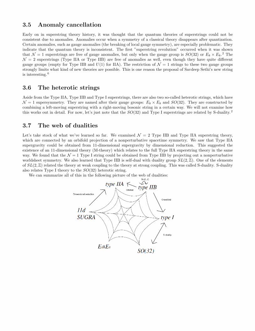
3.5 Anomaly cancellation
Early on in superstring theory history, it was thought that the quantum theories of superstrings could not beconsistent due to anomalies. Anomalies occur when a symmetry of a classical theory disappears after quantization.Certain anomalies, such as gauge anomalies (the breaking of local gauge symmetry), are especially problematic. Theyindicate that the quantum theory is inconsistent. The first ”superstring revolution” occurred when it was shownthat N = 1 superstrings are free of gauge anomalies, but only when the gauge group is SO(32) or E8 × E8.2 TheN = 2 superstrings (Type IIA or Type IIB) are free of anomalies as well, even though they have quite differentgauge groups (empty for Type IIB and U(1) for IIA). The restriction of N = 1 strings to these two gauge groupsstrongly limits what kind of new theories are possible. This is one reason the proposal of Savdeep Sethi’s new stringis interesting.6
3.6 The heterotic strings
Aside from the Type IIA, Type IIB and Type I superstrings, there are also two so-called heterotic strings, which haveN = 1 supersymmetry. They are named after their gauge groups: E8 × E8 and SO(32). They are constructed bycombining a left-moving superstring with a right-moving bosonic string in a certain way. We will not examine howthis works out in detail. For now, let’s just note that the SO(32) and Type I superstrings are related by S-duality.2
3.7 The web of dualities
Let’s take stock of what we’ve learned so far. We examined N = 2 Type IIB and Type IIA superstring theory,which are connected by an orbifold projection of a nonperturbative spacetime symmetry. We saw that Type IIAsupergravity could be obtained from 11-dimensional supergravity by dimensional reduction. This suggested theexistence of an 11-dimensional theory (M-theory) which relates to the full Type IIA superstring theory in the sameway. We found that the N = 1 Type I string could be obtained from Type IIB by projecting out a nonperturbativeworldsheet symmetry. We also learned that Type IIB is self-dual with duality group SL(2,Z). One of the elementsof SL(2,Z) related the theory at weak coupling to the theory at strong coupling. This was called S-duality. S-dualityalso relates Type I theory to the SO(32) heterotic string.
We can summarize all of this in the following picture of the web of dualities:

Chapter 4
Compactification
In the previous chapters we built the bosonic and supersymmetric string theories. We found that the bosonic stringlives in D = 26 and the superstring in D = 10. In order to make this consistent with reality, either all but 4 of thesedimensions have to be compactified. Compactification changes the predictions of the theories considerably. In thischapter we will discuss simple circular and toroidal compactifications, which entail that either one or two spatialcoordinates satisfy
Xµ ∼ Xµ + 2πR (4.1)
where R is the radius of the compactified dimension. The symbol ∼ indicates that the two points are identified.Compactifications were first introduced in Kaluza-Klein theory, which was an attempt to unify general relativitywith electrodynamics in 5-dimensional spacetime. The most simple effect of compactification we want to discuss isthe emergence of so-called Kaluza-Klein towers. These are towers of massive states coming from a field which isnormally massless. We will examine Kaluza-Klein towers in the context of 11-dimensional supergravity at the endof this chapter. Our first topic will be T-duality, which is a duality between a theory compactified on R and anothertheory compactified on α′
R . Objects called D-branes are required to appear in any theory with T-duality. D-branesare hyperplanes on which open strings may end. Just as a point particle acquires electric charge when it couples tothe one-form Maxwell gauge field, a string acquires charge when it couples to a two-form Kalb-Ramond gauge field.In general, a p-brane may couple electrically to a (p + 1)-form gauge field. This fact will be crucial in our analysisof orientifold planes in Chapter 5. This chapter contains information from Becker Becker Schwarz2, Zwiebach1, andDabholkar4.
4.1 T-duality and D-branes in the bosonic theory
4.1.1 Closed strings
We will start our exploration of these new concepts in the most simple way possible, focusing on closed bosonicstrings. A closed bosonic string compactified on a circle satisfies the following boundary conditions:
X25(σ + π, τ) = X25(σ, τ) + 2πRW (4.2)
where the index 25 denotes the single compactified dimension, R is the radius of the compactification, and W is aninteger known as the string’s winding number. The winding number indicates how many times the closed string iswrapped around the circle. We may indicate the geometry of the spacetime under consideration by (R24,1 × S1),where S1 stands for the circularly compactified dimension and R24,1 indicate the 24 noncompact spatial dimensionsand the time dimension. The new boundary conditions change the mode expansions for the X25 coordinates:
X25(σ, τ) = x25 + 2α′p25τ + 2RWσ + oscillators (4.3)
We can rewrite the third term slightly using:
w ≡ mR
α′(4.4)
We then obtain:X25(σ, τ) = x25 + 2α′p25τ + 2α′wσ + oscillators (4.5)
This seems to suggest that the winding modes and the momentum are on equal footing. Let’s explore this idea. Wecan split the expansion of X25 into left- and right-movers:
X2R5 =
1
2(x25 − x25) + (α′
K
R−WR)(τ − σ) + oscillators (4.6)
32

X2L5 =
1
2(x25 + x25) + (α′
K
R−WR)(τ + σ) + oscillators (4.7)
We can incorporate the first factors in the second term into the zero modes α250 and α25
0 :
√2α′α25
0 = α′K
R−WR (4.8)
√2α′α25
0 = α′K
R+WR (4.9)
In terms of these zero modes, find:
p25 =1√2α′
(α250 + α25
0 ) (4.10)
w =1√2α′
(−α250 + α25
0 ) (4.11)
which confirms our suspicion that w is a form of momentum. Because the x25 dimension is compactified, the valuesof p become quantized, just like the momentum states of a particle in a box:
p25 =K
R, K ∈ Z (4.12)
We see that we have a momentum inversely proportional to R and a momentum proportional to R. We could makethe guess that transforming R → α′/R and exchanging W ↔ N leaves the momentum spectrum invariant. Let’squantize the string and see if this suspicion is confirmed. The mass squared of the string is given by:
M2 = −24∑µ=0
pµpµ (4.13)
which receives no contributions from the momentum in the compactified dimension. The physical state conditions(L0 − 1) |phys〉 = 0 and (L0 − 1) |phys〉 = 0 appear essentially unchanged. They receive contributions from theoscillators of the compactified dimension as well. The mass-shell condition now becomes:
α′M2 = α′[(K
R)2 + (
WR
α′)2
]+ 2NL + 2NR − 4 (4.14)
subject to the level-matching conditionNR −NL = WK (4.15)
We see that the mass spectrum is invariant under the transformation R→ α′/R and the interchange W ↔ K. Thisis called T-duality. It is actually a symmetry of the full interacting theory of the bosonic string. In a slightly modifiedform, it relates several superstring theories to each other as well. Because T-duality maps a closed string theory toanother closed string theory, the closed string is self-dual. After compactification, the massless 26-dimensional tensorstates of the closed string in R25,1 rearrange themselves into 25-dimensional tensors. Among these are two one-formMaxwell gauge fields, a Kalb-Ramond field and a graviton. This is analogous to the situation in Kaluza-Klein theory,where compactification of a fifth dimension rearranges the five-dimensional metric gµν into a four-dimensional gmn,a vector gm5 (which is a Maxwell field), and a four-dimensional dilaton1.
We can express the transformations of T-duality in a different way:
XR → −XR, and XL → XL (4.16)
along with R→ α′/R. This is how T-duality will act on open strings as well (open strings can always be continuouslycontracted to a point, so they have no notion of winding number). We will examine open bosonic strings in a moment.First, we want to comment on why we think T-duality is an exact symmetry of bosonic string theory rather thanmerely a coincidental overlapping of spectra. The T-duality transformation introduces the dual coordinate X:
X = XL +XR → X = XL −XR (4.17)
We can define a momentum conjugate to the dual coordinate:
Pτ =1
2πα′(XL − XR) (4.18)
And we can postulate the following commutation relation:
[X(τ, σ),Pτ (τ, σ′)] = iδ(σ − σ′) (4.19)
which leads to the commutation relations:[x0, w] = i (4.20)
[x0, p] = [x0, αn] = [x0, αn] = 0, n 6= 0 (4.21)
[x0, x0] = 0 (4.22)
We want to find a mapping from the operators of the theory at radius R to the operators of the theory at radius α′/R.This mapping must respect all commutation relations and map one Hamiltonian into the other. This is satisfied bythe following mapping: (
x0 → x0
x0 → x0
),
(p→ ww → p
),
(αn → −αnαn → αn
)(4.23)
This constitutes a proof that the two theories are equivalent, at least before interactions are included. T-duality isactually an exact symmetry of the full interacting quantum theory1, but we will not attempt to prove this.
4.1.2 Open strings
The action of T-duality on open strings is the mapping of X onto its dual coordinate X, along with, of course,the inversion of the compactification radius R → α′/R. There is no interpretation in terms of winding numbershere, since Neumann open strings are topologically equivalent to a point. The expansion of a coordinate satisfyingNeumann boundary conditions is:
X(τ, σ) = x+ pτ + i∑n 6=0
1
nαne
−inτ cos(nσ) (4.24)
(with `s = 1). Splitting this into the left- and right-movers:
XR(τ − σ) =x− x
2+
1
2p(τ − σ) +
i
2
∑n 6=0
1
nαne
−in(τ−σ) (4.25)
XL(τ + σ) =x+ x
2+
1
2p(τ + σ) +
i
2
∑n 6=0
1
nαne
−inτ+σ (4.26)
Performing the T-duality transformation yields:
X(τ, σ) = x+ pσ +∑n 6=0
1
nαne
−inτsin(nσ) (4.27)
This is just the expansion of a coordinate satisfying Dirichlet boundary conditions! Specifically, the boundaryconditions become:
X(τ, 0) = x, and X(τ, π) = x+πK
R= x+ 2πKR (4.28)
The mode expansion for the dual string carries no momentum, but there now appears a winding number in theboundary conditions. The Dirichlet string is not topologically equivalent to a point, since the end points of the stringare fixed.
Dirichlet boundary conditions are problematic in two ways: Firstly, they break Poincare invariance. Secondly,the string momentum is not conserved. There needs to be a physical object to which the string ends are attachedin order to account for the momentum non-conservation. These objects are p-dimensional hyperplanes called Dp-branes, short for Dirichlet branes. We can simultaneously compactify and T-dualize other directions as well. Thecorresponding coordinates interchange Neumann and Dirichlet boundary conditions.

4.1.3 D-branes and gauge fields
Let’s consider the quantization of a string attached to a Dp-brane. The mode expansion for Dirichlet coordinatesconsidered above leads to the usual commutation relations for the oscillators. The mass shell condition becomes:
M2 =1
α′(−1 +
∞∑n=1
p∑i=2
nai†n ain) +
∞∑m=1
d∑a=p+1
maa†maam (4.29)
where p indicates the transverse coordinates which still satisfy Neumann boundary conditions. The second termsums over the Dirichlet coordinates. Note that we are working in light-cone gauge and that we have not assumed anycompactification. The ground state is now labeled by the momentum in the transverse Neumann directions (denoted~p), and the light-cone momentum p+. There is no total momentum in the Dirichlet directions. To summarize, theground state is labeled: ∣∣p+, ~p
⟩(4.30)
We build the Fock space by acting with oscillators normal to the brane or oscillators tangent to the brane. Thevarious fields may be assigned a Schrodinger wavefunction Ψi1,...,ip,a1,...,aq (τ, p
+, ~p). This indicates that the fieldslive on the Dp-brane world volume. The wavefunction has no dependence on momentum in directions normal tothe brane. The wavefunction may therefore be Fourier transformed from momentum space into the Dp-brane worldvolume1. This is the most natural interpretation, but of course the argument presented here does not constitute aproof.
We can see from the mass formula that the first excited states are massless. We can act with an oscillator tangentto the brane to obtain:
ai†1∣∣p+, ~p
⟩(4.31)
This is an SO((p + 1) − 2) massless vector boson. It constitutes a U(1) gauge field on the world volume of the
D-brane. Acting with the normal oscillators aa†1 yields a massless scalar for each Dirichlet direction. These statesrepresent displacements of the D-brane.
Let’s consider the case where we have N parallel Dp-branes. Each end of the open string may end on any oneof the D-branes, so the string obtains an additional N2 degrees of freedom. These degrees of freedom are sometimescalled Chan-Paton charges. They were introduced into string theory before the discovery of D-branes, as an algebraictool without a clear physical interpretation. We may include the Chan-Paton degrees of freedom with the indices[ij] in the ground states: ∣∣p+, ~p; [ij]
⟩(4.32)
Let’s focus on the case N = 2. For strings starting on one D-brane and ending on the other, the mass shell conditionbecomes:
M2 =1
α′(N − 1) + (
xa2 − xa12πα′
)2 (4.33)
where xai denote the positions of the D-branes. Let’s take a look at the first excited states. Acting with oscillatorsnormal to the brane, we get:
aa†1∣∣p+, ~p; [12]
⟩(4.34)
at first glance, these appear to be (d− p) massive scalar fields. For the tangent oscillators, we get:
ai†i∣∣p+, ~p; [12]
⟩(4.35)
these are (p− 1) massive states. In order to fit these into an SO(p) representation, as is required for vector bosonsby Wigner’s classification, we require an extra degree of freedom. This extra state can come from the scalar fields.A certain linear combination of scalar states becomes part of the vector, in what has been called a ”stringy Higgsmechanism”. When the separation between the D-branes is zero, we get the same particle content as in the casewhere the string starts and ends on the same D-brane. We therefore find N2 = 4 massless U(1) gauge fields. Theseactually interact with each other to form a U(2) massless gauge field. This is a general result: N coincident D-branescarry a U(N) massless gauge field on their world volume! If only N0 ≤ N of the D-branes coincide, we obtain aU(N0)× U(1)N−N0 gauge symmetry.2 These facts will be crucial when we consider orientifolds.
4.1.4 Wilson lines
In a compactified space, a potential with a vanishing field strength can have physical effects. These effects arecharacterized by a so-called Wilson line, which is a matrix U that breaks a U(N) gauge symmetry to its subgroup ofelements commuting with U . We will have to understand Wilson lines to know how T-duality works on configurationsof non-coincident D-branes.

Let’s first review what exactly we mean by a U(N) gauge symmetry. The easiest way to do this is to examine thegauge transformation of Maxwell’s equations, which have U(1) gauge symmetry. Consider the classical Hamiltonianfor a charged particle with mass m and charge q:
H =1
2m(~p− q ~A)2 + qΦ (4.36)
The Schrodinger equation becomes:
i∂ψ
∂t=
1
2m(∇i− q ~A)2ψ + qΦψ (4.37)
The Schrodinger equation is invariant under the following simultaneous transformations:
~A→ ~A′ = ~A+∇χ (4.38)
Φ→ Φ′ = Φ− ∂χ
∂t(4.39)
Φ→ Φ′ = eiqχΨ (4.40)
where χ(x) is a function of spacetime. Let’s denote the phase factor with U(x):
U(x) ≡ eiqχ(x) (4.41)
Now, remember that Maxwell gauge transformations are often expressed in the following way:
Aµ → A′µ = Aµ + ∂µχ (4.42)
where we interpret χ(x) as the gauge parameter. We will have to shift our viewpoint on this in order to work withgauge fields on compactified spaces. More fundamentally, it is U(x) that should be considered the gauge parameter.We can rewrite the gauge transformation as:
Aµ → A′µ = Aµ −i
q(∂µU)U−1 (4.43)
It is easy to see that U(x) is an element of U(1). In general, U(N) is the group of N-by-N unitary matrices, so anelement u of U(1) simply satisfies u∗u = 1. The argument is completed by noting that Maxwell gauge transformationsperformed in sequence satisfy the rules of group multiplication. In other words:
ψ(x)→ U2(x)ψ(x)→ U1(x)(U2(x)ψ(x)) = (U1U2)(x)ψ(x) (4.44)
Let’s return to the subject of Wilson lines. Consider a space Rn × S1 where the x dimension has been compactifiedinto a circle. A vector potential Ax = c where c is constant now satisfies all the field equations. A field with such avector potential has vanishing field strength, but may still have physical effects. A gauge transformation of Ax takesthe form:
Ax → Ax +∂χ
∂x(4.45)
Under the assumption that chi(x) is the gauge parameter, it would be natural to require:
χ(x+ 2πR)?= χ(x) (4.46)
We can now define the holonomy or Wilson line of the gauge field:
W ≡ exp(iw) = exp(iq
∮dxAx) (4.47)
The gauge transformation acts upon w as:
w → w′ = w + q(χ(x0 + 2πR)− χ(x0) (4.48)
where the integral has been taken around the circle once starting from an arbitrary point x0. If (4.46) is correct,then w does not change under the gauge transformation. If, however, we interpret U(x) as the gauge parameter,then it is U(x) that should be periodic on the circle:
U(x+ 2πR) = U(x) (4.49)
This implies that w′ = w + 2πm, with m ∈ Z, under gauge transformations. In other words, we should make theidentification:
w ∼ w + 2πm, m ∈ Z (4.50)
The natural interpretation is that w is really an angle of some kind. To emphasize this, let’s rewrite:
θ ≡ w = q
∮dxAx (4.51)
There are many choices of χ that are not single-valued on the circle, but do lead to a single-valued U(x). Thesimplest one is the following:
qχ = (2φm)x
2πR=mx
R, m ∈ Z (4.52)
A gauge transformation changes this field by mR . So we can make the identification:
qAx ∼ qAx +m
R(4.53)
When Ax is constant, we can write:
qAx =θ
2πR(4.54)
The presence of the Wilson line has significant physical effects. In particular, the energy levels of a charged particleare shifted according to:
En =1
2m
(n
R− θ
2πR
)2
(4.55)
as may be checked by solving the Schrodinger equation.Now let’s apply these ideas to D-branes. T-duality will provide a very simple physical interpretation to the angle
variable that specifies the Wilson line, relating it to the locations of D-branes along compactified circles.Consider a Dp-brane that wraps around the circular dimension x. After T-dualizing x, it is transformed into
a D(p − 1)-brane located at some point on the dual circle. We can see this from the fact that T-duality turnsNeumann boundary conditions into Dirichlet boundary conditions. Now let’s say the Dp-brane carried a gauge fieldthat satisified:
q
∮Axdx = θ (4.56)
It turns out that θ specifies the position of the D(p − 1)-brane along the dual circle! We can see this by addinganother Dp-brane to the configuration. Let’s say the Dp-branes now have gauge fields such that the angular variablesbecome θ1 and θ2. The momentum in the circular direction of a string stretched between the two D-branes is shiftedaccording to:
n
R→ n
R− θ2
2πR+
θ1
2πR(4.57)
with n ∈ Z because the momentum is quantized. This shift occurs due to the coupling of the string endpoints to theMaxwell field on the Dp-brane world volume. The mass-squared formula becomes1:
M2 =
(2πn− (θ2 − θ1)
2πR
)2
+1
α′(N − 1), n ∈ Z (4.58)
This in fact precisely coincides with the mass-squared formula for a string stretched between two D(p − 1)-branesin the T-dual description, as may be seen by comparing with (4.33). We have seen that the relative positions ofD-branes determine the structure of the gauge fields that live on their world volume. For example, N coincidentD-branes produce a U(N) gauge field, whereas only a U(N0)×U(1)N−N0 gauge symmetry is produced when N0 ≤ ND-branes are coincident. Wilson lines do in fact break gauge symmetry in the same way. For a general U(N) gaugefield, we can define the holonomy matrix, or Wilson line:
U ≡ expi
∫ 2πR
0
Adx (4.59)
where A is a hermitian matrix specifying the gauge potential, which may be transformed into diagonal form by aconstant gauge transformation:
A = − 1
2πRdiag(θ1, θ2, ...θN ) (4.60)
In the presence of this Wilson line, the U(N) gauge symmetry is broken to the subgroup of its elements that commutewith U .2 When all the eigenvalues of U are distinct, the symmetry is broken to U(1)N . Just like before, the θnvariables specify the positions of D(p− 1)-branes in the T-dual world.
We will encounter Wilson lines again when we discuss Type I’ superstring theory in the next chapter.

4.1.5 String charge
Our last topic before we move on to the superstring theory will be string charge. Just like a point particle may coupleelectrically to the Maxwell field and acquire a charge 1, a string may couple ”electrically” to the Kalb-Ramond field.To see how this works out, let’s look at the point particle action in the presence of a Maxwell field:
S = −m∫ds+ e
∫Aµ(x)dxµ − 1
4κ20
∫dDxFµνF
µν (4.61)
where κ20 is a constant with dimension MD−4, which is necessary in order to make the units work out. The second
term takes this form because the world-line is parametrized with a single variable τ , which defines a tangent vectordxµ/dτ that forms a Lorentz scalar when multiplied by the gauge field Aµ. Strings can couple to Kalb-Ramond fieldsin an analogous way. This time we have two tangent vectors ∂Xµ
∂τ and ∂Xν
∂σ , which may form a Lorentz scalar whenmultiplied by Bµν :
−∫dτdσ
∂Xµ
∂τ
∂Xν
∂σBµν(X(τ, σ)) (4.62)
This term in the action leads to a conserved vector charge that is tangent to the string, pointing in the direction ofincreasing σ.1
The previous discussion suggests that Dp-branes may also couple electrically to some tensor field. In the bosonictheory, this doesn’t work out for p > 1, because there is no three-form (or higher) field in the massless spectrum. Aswe already know, the superstrings do contain massless higher-form fields, which means the D-branes may acquire theirown ”electric” charge. This implies that D-branes can be stable in superstring theories, an issue that is more subtlein the bosonic theory due to the existence of tachyons. In the next section, we will generalize this discussion usingthe language of differential forms. The existence of D-brane charge will be crucial in our discussion of orientifolds.
4.2 T-duality and D-branes in superstring theory
We will now extend the previous considerations into superstring theory. When we add D-branes, open superstringsbecome a possibility. We mentioned in Chapter 2 that only N = 1 supersymmetry is consistent with open stringboundary conditions. Adding D-branes to Type II theory breaks at least half of the supersymmetries, along with theSO(1, 9) Lorentz symmetry, which is reduced to SO(1, p)×SO(9− p). The world volume of a single D-brane carriesa U(1) gauge field coming from the NS sector states bµ−1/2 |NS〉, where the index µ indicates the directions tangent
to the D-brane. This can be seen from quantizing the superstring under the appropriate boundary conditions. Itworks out exactly the same way as in the bosonic theory. A number N of coincident D-branes carry N interactinggauge fields which together form a U(N) gauge symmetry.
In Type II theory, D-branes can be stable. This is possible due to the presence of massless higher-form gaugefields to which the D-branes may couple elecrically (or, as we will see, magnetically).
4.2.1 D-brane charges
To see this, we need to revisit our previous discussion of string charge, this time using the language of differentialforms. In general, an n-form gauge field in the is given by:
An =1
n!Aµ1µ2...µndxµ1 ∧ dxµ2 ∧ ... ∧ dxµn (4.63)
The field strength is given by Fn+1 = dAn. This field strength has a gauge invariance δAn = dΣn−1 where Σn−1 isan (n - 1)-form. This follows from the fact that the square of an exterior derivative equals zero.
Let’s take a look at what Maxwell theory looks like expressed in differential forms. The free field equationsbecome:
dF = 0 (4.64)
d ? F = 0 (4.65)
where ?F represents the Hodge dual of F . The hodge dual of an n form in D dimensions is a (D− n)-form.2 Whenwe incorporate sources, the field equations become:
dF = ?Jm (4.66)
1We have already seen that string endpoints do in fact couple to Maxwell fields. However, the two endpoints carry opposite charge,so a string as a whole is neutral with respect to a Maxwell field

d ? F = ?Je (4.67)
where Je and Jm are one-forms proportional to the current density Jµ = (ρ,~j). These equations presume magneticmonopoles exist, even though they have not been discovered yet. In D = 4, we can calculate electric and magneticcharges in the following way:
e =
∫S2
?F (4.68)
g =
∫S2
F (4.69)
where e is the electric charge and g is the magnetic charge. S2 indicates that the integral is to be carried out over atwo-sphere surrounding the sources. Dirac discovered that electric and magnetic charge have to be connected by aquantization condition:
e · g ∈ 2πZ (4.70)
We can generalize the above discussion to higher dimensions to investigate D-brane charges. Remember thatpoint particles may couple electrically to Maxwell fields because of the presence of the following term in the action:
Sint = e
∫Aµdx
µ = e
∫dτAµ
dxµ
dτ(4.71)
That this leads to an electric charge e may be checked by taking a variation of Aµ, which leads to a continuityequation. The result is consistent with the integration of the field strength hodge dual over the two-sphere. In thegeneral case, the integration must be carried out over a (D− 2)-sphere, because of hodge dual of the field strength isitself a (D− 2)-form. The magnetic charge is calculated by the integration over the field strength, which in the caseof the Maxwell field is a two-form. In D-dimensions, a two-sphere S2 can surround a (D − 4)-dimensional object.For example, R9,1 the D6-branes carry magnetic charge with respect to the Maxwell field.
Let’s generalize further to incorporate higher-form fields. The electric coupling of an n-form field now occurs tothe world volume of an (n− 1)-brane. This is reflected in the following term in the action:
Sint = µp
∫Ap+1 (4.72)
where µp represents the p-brane charge. This integral can be rewritten:∫Ap+1 =
1
(p+ 1)!
∫Aµ1...µp+1
∂xµ1
∂σ0...∂xµp+1
∂σPdp+1σ (4.73)
That this leads to an electric charge µp can be verified by taking a variation to obtain a continuity equation. Theresult is consistent with the integration µp =
∫?Fp+2, which must now be carried out over a (D − p − 2) sphere.
Likewise, the n-form gauge field may couple magnetically to the (D − p − 4)-brane. The higher-form gauge fieldcharges have to satisfy a Dirac quantization condition as well. In ten dimensions, this becomes2:
µpµ6−p ∈ 2πZ (4.74)
4.2.2 Stability of D-branes
Let’s take a look at which D-branes, specifically, couple to which fields in the Type II massless spectra. As we’vediscussed before, a charged D-brane must be stable. In the Type IIA massless spectrum, we find the one-form A andthe three-form C3. These couple electically to D0-branes (which are point particles), and D2-branes, respectively.They couple magnetically to D6- and D4-branes. Altogether, this implies the stability of the Dp-branes with p =0, 2, 4, 6. This regularity suggests that D8-branes might be stable as well. A D8-brane would couple electrically toa nine-form gauge field. Such a field is nondynamical, because its field equation dF10 = 0 is automatically satisfieddue to the anti-symmetry of wedge products. Similarly, in Type IIB theory, we find that Dp-branes with odd p areguaranteed to be stable, although the analysis is rather more subtle in this case.2
The presence of stable D-branes reduces the supersymmetry to N = 1. For this reason, they are sometimesreferred to as half-BPS D-branes. The requirement of supersymmetry decouples the tachyon from the open stringspectrum. D-branes which do not have the right dimensionality to couple to a gauge field are not protected by aconserved charge and are therefore unstable. They break the full supersymmetry of the theory. This leaves openstrings attached to them free to carry a tachyon. An unstable D-brane can decay into closed-string radiation.
The inclusion of D-branes in Type II theory is actually necessary in order to keep the SL(2,Z) symmetry of TypeIIB.4 As we mentioned in the last chapter, nonperturbative dualities can be tested by investigating the spectrum
of BPS states. It can be shown that a string wound around a compactified direction is charged with respect to B2.Such a string is in a BPS state if it carries no momentum in the compactified direction. Under the element S ofSL(2,Z), the fields B2 and B′2 are transformed into each other, so in order for SL(2,Z) to hold, we need to findstates which are charged with respect to B′2. There are no such string states in the BPS spectrum due to a generalrule that perturbative states couple to the field strength of R-R fields and not to the potential. However, the B′2may also couple to D1-branes. If we include these into the theory, the SL(2,Z) symmetry is saved. The D1-brane issometimes referred to as the D-string.
4.2.3 Type II T-duality
T-duality mapped the theory of closed bosonic strings on R to the same theory on α′/R. We therefore said thatclosed bosonic string theory is self-dual under T-duality. The closed strings of Type II superstring theory, however,are not self-dual. T-duality actually maps a IIA string on R to a IIB string on α′/R. We will examine how thisworks out in this subsection.
Let’s take type II theory with one direction, X9, say, compactified on a circle of radius R. The action of T-dualityon the bosonic coordinates is exactly the same as before:
X9L → X9
L, and X9R → −X9
R (4.75)
In the RNS formalism, the same thing happens to the fermion ψ9:
ψ9L → ψ9
L and ψ9R → −ψ9
R (4.76)
This flips the chirality of the right-moving R-sector fermion. To see this, note that the transformation flips the signof the zero modes:
d90 → −d9
0 (4.77)
In the previous chapter we saw that the R-sector zero modes furnish a representation of the Dirac algebra, whichmay be expressed as:
Γµ =√
2dµ0 (4.78)
So the transformation takes Γ9 into −Γ9, which also flips the sign of the chirality operator Γ11. The differencebetween Type IIB and Type IIA theory was in the relative chirality of the left- and right-moving R sector fermions.We therefore see that T-duality maps IIA into IIB and vice versa. This fact will be of use to us when we examinethe M-theory description of Savdeep Sethi’s new string.
Just like in the bosonic theory, the transformations of T-duality interchange Neumann and Dirichlet boundaryconditions of open strings. This implies that T-duality transforms Dp-branes into D(p− 1)-branes. This means thatthe stable half-BPS D-branes of Type IIB get transformed into the stable half-BPS D-branes of Type IIA (and viceversa), which is what we would like to see.
In the GS formalism in light-cone gauge, the T-duality transformations for Type IIB take the following form:
Sa1 → ΓΓ9Sa (4.79)
Sa2 → Sa2 (4.80)
where Γ = Γ1Γ2...Γ8. This flips the chirality of the right-moving fermions. We get a left-moving conjugate spinor 8cand a right-moving spinor 8s, so T-duality maps IIB into IIA as expected.2
Lastly, let’s see how T-duality transforms the perturbative symmetries of Type IIB theory. We obtain thefollowing4:
Ω in IIB → I9Ω in IIA (4.81)
where I9 is given by:I9 : (X9
L, X9R)→ (−X9
L,−X9R) (4.82)
The action of I9 on the fermions is to flip the chirality of both of them. Ω by itself is of course not a symmetry ofType IIA theory, because it takes a theory with a left-moving spinor and right-moving conjugate spinor into a theorywith right-moving spinor and a left-moving conjugate spinor. I9 flips them back and we obtain a proper symmetryof Type IIA.
4.3 Kaluza-Klein towers and 11-dimensional supergravity
When we compactify a D-dimensional theory, a field which is ordinarily massless may appear to be massive in thedimensionally reduced theory. For example, let’s take a massless scalar φ in a D-dimensional theory. When wecompactify down to (D − 1) dimensions, the field may be Fourier expanded on the circular coordinate:
φ(~x, 0) =
∞∑n=−∞
φ(n)(~x)einθ/R (4.83)
where θ represents the circular coordinate, R is the radius of compactification, and ~x indicate the D− 1 noncompactdimensions. The field satisifies the D-dimensional Klein-Gordon equation on the full spacetime:
∂µ∂µφ = 0 (4.84)
More explicitly:(∂A∂A + ∂θ∂θ)φ(~x, θ) = 0 (4.85)
where the index A indicates the noncompact dimensions. Carrying out the derivatives with respect to θ and takingthe perspective of an observer in the lower-dimensional spacetime, the equation becomes:
(∂µ∂µ −N2
R)φ(~x), N ∈ Z (4.86)
which is just the Klein-Gordon equation for a massive scalar. We therefore see that a whole tower of massive statesemerges from the compactification. This is called a Kaluza-Klein tower. We will apply the previous analysis tothe dimensional reduction of 11-dimensional supergravity. The field under consideration will be the full masslesssupergraviton. We will find that there is a duality between M-theory compactified on a torus (S1 × S1) and TypeIIB superstring theory compactified on a circle S1.
4.3.1 A note on BPS states
Before we can proceed, we want to clarify some of our discussion about BPS states. These are states that are partof a so-called shortened supersymmetry multiplet. Their mass is tied to a conserved charge of a massless gaugefield. More explicitly, in supersymmetry theories (not specific to string theory) there is a so-called central-chargematrix, whose elements ±Zi (with |Z1| ≥ |Z2| ≥ ... ≥ 0) are electric and magnetic charges belonging to the masslessgauge fields of the theory. Crucially, these charges commute with all the generators of the supersymmetry algebra.These generators realize the supersymmetry transformations given in the previous chapter, and as such they squareto spacetime translations. The matrix (
M ZZ† M
)(4.87)
is required by the supersymmetry algebra to be positive semidefinite. This implies that the eigenvalues of this matrixM ± |Zi| are nonnegative. This implies that the mass of the states is bounded below2:
M ≥ |Z1| (4.88)
All of this is still rather abstract at this point. The only way to clarify the discussion is to delve deeper into themathematics of supersymmetry theories, which we do not have time for. The important part is the following: thestates which have M = |Z1| are the BPS states. They are protected by supersymmetry from quantum corrections. Inother words, we can reliably extrapolate their weak-coupling mass formulas to strong coupling. This is what makesthem so useful for analyzing proposed dualities. If we can establish that a duality holds among the BPS states, itprovides evidence that the duality holds in the full theory, including at strong coupling.
4.3.2 M-theory - Type II duality
We’ve seen that 11-dimensional supergravity compactified on a circle gives Type IIA supergravity, which suggestedthat the same link exists between M-theory and the full Type IIA superstring theory. We’ve also seen that TypeIIA compactified on a circle R is equivalent under T-duality to Type IIB compactified on the dual circle α′/R. Thisseems to suggest that there exists a duality between M-theory compactified on a torus and Type IIB on a circle. Wewill now try to verify this.
As we noted earlier in this chapter, the SL(2,Z) symmetry may transform the fundamental string of Type IIBtheory (the F-string, which couples electrically to B2) into the D-string (which couples to B′2), or vice versa. The
transformation is more general than that, and we obtain a whole tower of (p, q) strings, where p indicates their chargewith respect to B2 and q indicates their charge with respect to B′2. The (p, q) strings are all supersymmetric, whichuniquely determines their tensions. The result is2:
T(p,q) = |p− qτb|TF = TF
√(p− q θ0
2π)2 +
q2
g2s
(4.89)
where τb is equal to the vacuum expectation value of the axion-dilaton field τ :
τb =< τ >=θ0
2π+
i
gs(4.90)
In general, a string’s tension is related to `s by:
T =1
2π`2s(4.91)
We have rewritten the axion C0 into an angular variable θ0 to emphasize its periodicity. Remember that the SL(2,Z)acts upon τ as:
τ → aτ + b
cτ + d, ad− bc = 1 (4.92)
which implies that C0 ∼ C0 + 1. This fact will be crucial to us later on, when we introduce Savdeep Sethi’s newsuperstring. As can be seen from the above formula, SL(2,Z) takes a theory at weak coupling to a theory atstrong coupling, so at most one of the (p, q) strings may be weakly coupled at the same time. Let’s write down theweak-coupling mass spectrum of Type IIB on a circle:
M2B = (
K
RB)2 + (2πRBWT(p,q))
2 + 4πT(p,q)(NL +NR) (4.93)
subject to the level-matching condition:NR −NL = KW (4.94)
We want to consider the spectrum of all the (p, q) strings at once and compare it to the Kaluza-Klein spectrumof 11-dimensional supergravity on a torus. However, the mass formula is meaningless at strong coupling due toquantum corrections, and at most one of the (p, q) strings is weakly coupled. The solution is to focus on just theBPS states. Their mass formulas are protected by supersymmetry and don’t receive quantum corrections. The BPSstates are those with NL = 0 or NR = 0. We can map the three integers W ,p, and q into two integers n1 and n2 inthe following way:
(n1, n2) = (Wp,Wq) (4.95)
where W is the greatest common divisor of n1 and n2. We can therefore specify all the BPS using K, n1, n2, andthe left-moving oscillator structure satisfying NL = |WK|. We can rewrite the second term in the mass formula as:
(2πRBWT(p,q))2 = (|n1 − n2τB |TF )2 (4.96)
Now let’s look at the M-theory Kaluza-Klein spectrum that results from the torus compactification. A torus may bespecified by two complex periods w1 and w2, which define the identifications
z ∼ z + w1, z ∼ z + w2 (4.97)
This defines a parallelogram on the complex plane, whose opposite edges are identified. The real and imaginary axesrepresent the two directions which will become the torus after compactification. We obtain the same parallelogramwhen we switch to the alternative periods w′1 and w′2:
w′1 = aw1 + bw2, w′2 = cw1 + dw2 (4.98)
with a, b, c, d ∈ Z and ad− bc = 1. In other words, the constants fit into a 2-by-2 matrix with determinant 1. We seethat the alternative torus periods fit into a group isomorphic to SL(2,Z). This is called the modular group of thetorus.
Let’s take a torus with periods w1 = 2πR11 and w2 = 2πR11τM , where τM is called the complex structure6.Under the torus identifications specified by these periods, we see that a single-valued wave function takes the form:
ψn1,n2 ∼ exp
[i
R11(n2x−
n2ReτM − n1
ImτMy)
](4.99)

In the same way we obtained the Kaluza-Klein tower for the massless scalar, the tower can now be obtained bytaking the derivatives in the compactified directions. The result is:
M2KK =
1
R211
[n2
2 +(n2ReτM − n1)2
(ImτM )2
]=|n1 − n2τM |2
(R11ImτM )2(4.100)
If we make the identification τM = τB , this is identical to the winding-mode term in the Type IIA mass formula, upto a normalization constant. The discrepancy in the normalization is due to the fact that these spectra are measuredin different metrics. This result confirms our suspicion that there exists a duality between M-theory on a torus(S1×S1)×R8,1 and Type IIB on (S1)×R8,1. It also implies that the SL(2,Z) symmetry of compactified Type IIBhas an elegant M-theory interpretation as the modular group of a toroidal compactification2.
4.4 The web of dualities: part II
Let’s summarize what we’ve learned about the web of dualities in this chapter. We now know that Type IIA andType IIB compactified on a circle are equivalent to each other under T-duality. We’ve also seen that there is a dualitybetween Type IIB on a circle and M-theory on a torus. It turns out that T-duality links the two heterotic stringsSO(32) and E8 × E8 as well (although we haven’t discussed this). To summarize:
The link coming from the center of this web represents a connection to M-theory.

Chapter 5
Orbifolds and Orientifolds
A number of times throughout the previous chapter, we’ve mentioned orbifold and orientifold projections. Theseprojections truncate a theory’s spectrum down to the states which are invariant under a certain symmetry. By doingso, we can often obtain the spectrum of a different consistent string theory. For example, we’ve suggested that Type Isuperstring theory may be obtained from Type IIB by keeping only the states which are invariant under world-sheetparity. This is not the whole story. For orbifolds, we need to add a sector of strings which satisfy boundary conditionsthat are twisted by an element of the orbifold group. For orientifolds, we need to deal with orientifold planes. Anorientifold plane is the set of points that are invariant under the subgroup of spacetime symmetries in the orientifoldgroup. Like D-branes, they can couple to gauge fields to acquire a charge. This charge must be cancelled by addingthe right number of D-branes carrying opposite charge. Just like Type I, Savdeep Sethi’s superstring is obtainedfrom Type IIB by an orientifold projection. We will see how this works out in Chapter 6.
5.1 General features of orbifolds
As a warmup to the subject of orientifolds, we first discuss orbifolds, which are a bit simpler. In mathematics,an orbifold is obtained from a smooth manifold with discrete isometry group G by identifying all points which aretransformed into each other by the action of an element of G. For example, we can obtain the orbifold S1/Z2 byidentifying the points x ∼ −x on a circle S1. The result is a line interval.2 We will not go any further into thegeometrical interpretation of orbifolds. For our purposes, an orbifold A′ is a theory which is obtained from a theoryA with discrete spacetime symmetry group G by projecting onto states which are invariant under G. Symbolically:
A′ = A/G (5.1)
In closed string theory, we need to add a so-called twisted sector. In the twisted sector, we find strings which areclosed up to an element α of the orbifold group G:
Φ(σ + 2π, τ) = αΦ(σ, τ) (5.2)
We must perform the projection onto G-invariant states in both the twisted and the untwisted sector4.
5.2 Type IIA as an orbifold
Let’s look at an example of an orbifold projection. As we discussed in Chapter 3, Type IIA superstring theorymay be obtained from Type IIB by projecting onto states invariant under the perturbative symmetry (−1)FL . Thisoperator clearly squares to 1, so the orbifold group will be isomorphic to Z2.
In the untwisted sector, the projection removes all R-NS and R-R states, which have odd left-moving fermionnumbers. The NS-NS and NS-R states all survive. In the language of group theory, we now obtain a masslessspectrum given by:
8v ⊕ (8v ⊕ 8c) (5.3)
In the twisted sector, the boundary conditions (in the GS formalism) become the following:
S1a(σ + 2π) = (−1)FLS1a(σ) = −S1a(σ) (5.4)
S2a(σ + 2π) = S2a(σ) (5.5)
44

The situation is unchanged for the right-movers. We obtain a ground state which transforms as 8v⊕8s. For the left-movers, the ground state actually becomes tachyonic due to the twisted boundary conditions. This isn’t a problem,because the ground state is projected out by the orbifold projection. The first left-moving excited state is given by:
Sa−1/2 |0〉 (5.6)
where the operator now carries a half-integer index due to the anti-symmetric boundary conditions. These states aremassless. They transform as:
8s⊗ (8v ⊕ 8c) (5.7)
Altogether, we obtain the following massless spectrum4:
(8v ⊕ 8s)⊕ (8v ⊕ 8c) (5.8)
which is just the Type IIA massless spectrum derived in Chapter 3.
5.3 General features of orientifolds
The difference between orientifolds and orbifold is that an orientifold group can contain world sheet orientationreversal Ω as well as spacetime symmetries. We can write this as:
G = G1 ∪ ΩG2 (5.9)
where G1 and G2 are spacetime symmetry groups. When G2 is non-empty, Ω becomes a local gauge symmetry, soafter the orientifold projection the theory only includes unoriented surfaces.
The set of points in spacetime which are left invariant under G2 form the orientifold plane2. Like a Dp-brane, ap-dimensional orientifold plane (an Op-plane) may couple to an R-R (p + 1)-form. This means that the orientifoldplane may be charged with respect to those fields. If it is charged, then it acts as a source term for the field equationsof the (p+ 1)-form Ap+1:
dHp+2 = ?J7−p (5.10)
d ? Hp+2 = ?Jp+1 (5.11)
where Hp+2 is the field strength of Ap+1 and Jn are the source terms. Consistency now requires that:∫Σk
?J10−k = 0 (5.12)
for all closed surfaces Σk. In a compact space, this is analogous to the fact that electric field lines coming from acharge must end on an opposite charge.4 The only way to cancel the contribution of the Op-plane charge to theabove integral is to add the appropriate number of Dp-branes carrying opposite charge.
5.4 Type I as an orientifold
Let’s see how the Type I superstring emerges from an orientifold projection of Type IIB theory. The relevantsymmetry in this case is world-sheet parity:
Ω : σ → −σ (5.13)
The orientifold group is now isomorphic to Z2, because we are not using any spacetime symmetries. This amountsto choosing the trivial group for G1 and G2. We’ve already examined the action of Ω upon the particle content ofthe Type IIB massless spectrum. In the NS-NS sector we keep the dilaton and the graviton. From the NS-R andR-NS sectors, we keep only the symmetric combination of gravitino fields (Ψµ
1 + Ψµ2 ) and one of the dilatinos. In
the R-R sector we keep only the two-form C2 and discard C0 and D4. We can now see this by counting degrees offreedom. The Type I theory is required to be supersymmetric, so we need to have an equal number of fermionic andbosonic degrees of freedom. The gravitino and dilatino, which are fermions, have 56 + 8 = 64 combined degrees offreedom. This is equal to the number of combined degrees of freedom of the graviton, dilaton, and the two-form C2,so we see that the above choice is correct. This is the content of the untwisted sector.
Because G2 is the trivial group (consisting of only the identity element) in this case, the entire spacetime isinvariant under its action. The orientifold plane becomes a 9-plane. It can couple to a 10-form R-R sector field(these do not appear after quantizing the spectrum because they are nondynamical). It can be shown that theorientifold plane carries -32 units of charge with respect to this field. We can cancel this by adding 32 D9-branes,
each of which has unit charge. These 32 D9-branes carry a U(32) massless gauge field on their world volume. Aftercarrying out the orientifold projection, only an SO(32) gauge symmetry remains. This is just what is necessary inorder to make gauge anomalies disappear!4
Because the only massless R-R field in the Type I spectrum is C2, the only stable Dp-branes (apart from theD9-branes) are the D1-brane (which couples to C2 electrically) and the D5-brane (which couples magnetically). TheType I fundamental string itself does not couple to any field (the B2 Kalb-Ramond field is discarded by the orientifoldprojection), so it isn’t stable. Fundamental Type I strings are only long-lived at weak coupling.2
5.4.1 Type I’
We know that Type IIA on R8,1 × S1 is T-dual to Type IIB on R8,1 × S1, where S1 indicates the dual circle. Thissuggests that taking an orientifold of Type IIA will yield a theory that is T-dual to Type I on R8,1×S1. This T-dualcounterpart of Type I is known as Type I’ or Type IA superstring theory.
Let’s take a look at the T-dual description of Type I. The T-duality transformation in Type II theory may beexpressed as:
X9R → −X9
R, and ψ9R → −ψ9
R (5.14)
X9 = X9L +X9
R → X9 = X9L −X9
R (5.15)
where X9 lies along the circle S1. In the Type I theory, world-sheet parity Ω is gauged. Ω exchanges left- andright-movers, so after the T-duality transformation it corresponds to
X9 → −X9 (5.16)
We have previously denoted this coordinate inversion as I9. The gauging of Ω actually requires us to identifyX9 ∼ −X9, which describes an orbifold of the dual circle. As discussed in Chapter 3, we can combine Ω and I9 into asymmetry of Type IIA. We can therefore form an orientifold group out of these two operations. T-duality now entailsthat the compactified Type IIB orientifold (R8,1×S1)/Ω is equivalent to the Type IIA orientifold (R8,1× S1)/Ω · I9.The set of points that are invariant under I9 form two 8-dimensional hyperplanes located at X9 = 0 and X9 = πR,where R is the radius of the dual circle. Each of these planes carries -8 units of R-R charge. This charge needs tobe cancelled by adding 16 D8-branes along the circle. In the rest of the thesis, we will place 8 D8-branes at each ofthe two orientifold planes. This configuration is dual to Type I with a Wilson line breaking the gauge symmetry toSO(16)× SO(16).5
5.5 Heterotic-Type I S-duality
The field contents of Type I and SO(32) heterotic supergravity are exactly the same. Moreover, their actions aremapped into each other by an inversion of the dilaton:
φ→ −φ (5.17)
combined with a Weyl rescaling of the metric gµν → e−φgµν . Since the string coupling is given by gs = e−φ,this suggests that the SO(32) and Type I superstrings are related by S-duality. This is verified by a number ofnonperturbative tests.2 The heterotic-Type I S-duality has a very nice interpretation as a classical symmetry ofM-theory compactified on a torus. This was discovered by Horava and Witten in 19955. Let’s briefly outline theirargument.
The low-energy limit of M-theory on the familiar Z2 orbifold R9,1×S1/Z2 is a ten-dimensional supergravity theorywith N = 1 chiral supersymmetry. There are three supergravities with this structure: Type I, E8 ×E8, and SO(32)heterotic. The low-energy limit of M-theory on the orbifold must converge to one of these nodes. By examiningthe strong coupling limit, the SO(32) and Type I supergravities may be ruled out. In the strong coupling limit,the compactification radius becomes very large. Far from the fixed hyperplanes of the orbifold, the strongly-coupledtheory is indistinguishable from strongly-coupled Type IIA, which is just M-theory on R9,1 × S1. We know that thestrongly-coupled limits of Type I and SO(32) heterotic are related to each other’s weakly-coupled limit by S-duality.This rules out the possibility that M-theory on the orbifold reduces to SO(32) heterotic or Type I. E8 ×E8 has (atthe time Witten and Horava published their article) previously unknown strong coupling behaviour, so it can’t beruled out. This suggests that M-theory on R9,1 × S1/Z2 is E8 × E8 superstring theory.
As discussed in the previous section, the T-dual of Type I superstring theory on R8,1 × S1 is related to the TypeIIA orientifold R8,1 × S1/Z2, which is called Type I’. Because Type IIA is just M-theory on R9,1 × S1, we hope thatM-theory on R8,1 × S1/Z2 × S1 is equivalent to Type I’ on a R8,1 × S1. On the other hand, we have argued thatM-theory on R8,1 × S1 × S1/Z2 is E8 × E8 on R8,1 × S1. From the M-theory perspective, it is quite transparent

that these two theories should be dual to each other. We don’t presently know what form this duality should takein the superstring theory. For starters, the two theories have completely different gauge groups. Witten and Horavaargue that the natural solution would be to turn on a Wilson line in the E8 × E8 theory, to break the gauge groupto SO(16) × SO(16).12 It is possible that the two theories are equivalent after turning on the Wilson line. Thisis not like any of the dualities we’ve seen before. We can relate it to a more familiar duality by T-dualizing boththeories. The Type I’ theory will turn into Type I on R8,1×S1. The E8×E8 theory will turn into SO(32) heterotic(with broken gauge symmetry SO(16)× SO(16) in each case). Now, we know that SO(32) heterotic and Type I areS-dual to each other. The suggestion is that the M-theory symmetry of exchanging the circles manifests itself as theS-duality in the superstring theory. A simple calculation (carried out in the paper by Horava and Witten) confirmsthis.
The exchange of S1 and S1/Z2 may actually be implemented by an element of SL(2,Z) acting upon the torus.Specifically, the element that takes
τM → −1
τ(5.18)
exchanges S1 and S1/Z2. It inverts the string coupling, and exchanges SO(32) heterotic string theory and Type I6.
5.6 The web of dualities: part III
Let’s update the web of dualities again. We have learned that Type IIA follows from Type IIB by a Z2 orbifold of(−1)FL , which we already mentioned in Chapter 2. Likewise, Type I superstring theory is obtained from Type IIBby an orientifold of world-sheet parity. The T-dual theory of Type I, called Type I’, is obtained by orientifoldingwith the combined operation of world-sheet parity and spacetime orientation reversal. We also know that TypeI’ on a circle is obtained from M-theory on R8,1 × S1 × S1/Z2. Similarly, E8 × E8 is obtained from M-theory onR8,1 × S1/Z2 × S1. A T-duality transformation on both of these yields SO(32) heterotic and Type I superstringtheory, which are related by S-duality. Let’s summarize with a picture:
1Remember that we are working with Type I’ with 8 D8-branes located at each orientifold plane. This is the T-dual of Type I with aWilson line breaking the gauge symmetry to SO(16)×SO(16). This has to be done because T-duality actually links E8×E8 with brokenSO(16) × SO(16) symmetry to the SO(32) string with broken SO(16) × SO(16) symmetry. The heterotic strings with full unbrokengauge symmetry are actually self-dual under T-duality.
2It should be clear that the difference implied by writing R8,1 × S1 × S1/Z2 instead of R8,1 × S1/Z2 × S1 lies in the ordering ofapplying the orbifold and the circular compactification.

Chapter 6
Savdeep Sethi’s Superstring
6.1 A different orientifold
We are finally ready to introduce Savdeep Sethi’s superstring. After all this introduction, it will seem like an almostdisappointingly simple proposal. Let’s reiterate some of our previous discussion. The SL(2,Z) symmetry of TypeIIB acts on the axion-dilaton field τ ≡ C0 + i
gs= C0 + ie−φ as:
τ → aτ + b
cτ + d(6.1)
The choice (a, b, c, d) = (1, 1, 0, 1) satisfies ad− bc = 1 and requires us to identify:
C0 ∼ C0 + 1 (6.2)
Type I superstring theory is obtained by taking an orientifold with world-sheet parity Ω of Type IIB. The axion C0
is odd under Ω:ΩC0 = −C0 (6.3)
so ordinarily the orientifold projection would require C0 = 0. However, C0 = − 12 is identified with C0 = + 1
2 underSL(2,Z). There is therefore a second possibility of orientifolding around C0 = 1
2 ! This is the new superstring.6
There are several things that can go wrong at this point. Firstly, the proposed theory might end up being equivalentto Type I superstring theory. Secondly, the theory might be inconsistent. The last possibility is that the theory isconsistent, but doesn’t fit into the web of M-theory backgrounds. An example of such a theory is massive Type IIAsupergravity. It will not be possible for us pick out one these possibilities with certainty. We will try to rule outthe first possibility, by comparing the BPS spectra of Type I and the new string from the perspective of M-theory.Secondly, we will take a look at the strong-coupling limit of the new superstring, which appears quite different fromType I’s strong-coupling limit (which is described by SO(32)’s weak-coupling limit).
6.2 M-theory BPS spectrum
Let’s look at the M-theory description of the Type I superstring. The simplest way to do this is to first compactifyon a circle and performing a T-duality transformation to Type I’. As we saw in the last chapter, this is describedby M-theory on R8,1 × S1 × S1/Z2. The orientifold uses the combined action of world-sheet and spacetime parity, Ωand I. We can describe the two circles by using angular coordinates (θ1, θ2). As we noted in Chapter 3, M-theoryhas a massless three-form A3. This field is odd with respect to world-sheet parity. The coordinate θ2 is of courseodd with respect to I. The orientifold produces two O8-planes corresponding to the set of points left invariant byits spacetime part. Their charge has to be cancelled by 16 D8-branes distributed across the circle.
Let’s reiterate our discussion about the Type IIB/M-theory duality. A torus is specified using two periods w1
and w2. We can normalize one of these to unity by rescaling the torus metric. We now have the periods w1 = 1 andw2 = τM . To obtain Type IIB theory, we have to identify τM with the axion-dilaton field expectation value τB . Wewill just call both of these τ from now on. Moreover, we define:
τ1 ≡ Reτ (6.4)
τ2 ≡ Imτ (6.5)
48

The torus identifications have become:z = θ1 + iθ2 ∼ z + (n+ mτ) (6.6)
with integer (n, m), and we are working with the torus metric:
ds2 =A
τ2dzdz (6.7)
where A is the area of the torus, which is given by:
RB =`3pA
(6.8)
where `p is the 11-dimensional Planck scale.We can express the Kaluza-Klein spectrum coming from the supergravity multiplet as follows:
M2(n,m) =
1
Aτ2[n2τ2
2 + (m− τ1n)2] (6.9)
which is just the same formula we obtained in Chapter 4, but expressed in a different way. Each of these modes, ofcourse, is BPS. From the Type IIB perspective, the interpretation of the (n,m) mode is an (n,m) string wrappedon a circle with radius RB . This is just what we saw in Chapter 4.
Let’s examine the action on the M-theory torus (with τ1 = C0 = 0) of the orientifold that produces Type I’superstring theory:
I : (θ1, θ2, A3)→ (θ1,−θ2,−A3) (6.10)
Only states which are invariant under this quotient action survive. This forces states with Kaluza-Klein momenta(0,m) to appear in combination with (0,−m). From the Type I perspective, this is just the statement that there areno stable fundamental string winding modes, due to the absence of an NS-NS two-form.
The question is now how the new string appears in M-theory. What really needs to be done is to study theperturbative orientifold with C0 = 1
2 and deduce its behaviour under T-duality. Unfortunately, we are unable todo this. The best we can do is guess that the quotient action should be unchanged. The T-duality between TypeI and Type I’ is straightforward, so it is unlikely to be affected by the expectation value of C0. This implies thatI takes θ2 → θ2, as before. The precise statement of the T-duality under consideration here is that Type I withbroken SO(16) × SO(16) gauge symmetry is dual to Type IIA on an orientifold with 8 D8-branes coincident witheach orientifold plane. Savdeep Sethi argues that the situation at the orientifold planes may be different for the newstrings. We have to keep this in mind in what follows.
The torus identifications (6.6) are invariant under the quotient action for both τ1 = 0 and τ1 = 12 . The natural
conclusion is that the second possibility corresponds to the new string. However, the quotient action on this newtorus produces only a single boundary for an orientifold plane to be located.At the boundary we find only a single setof SO(16) gauge bosons, whereas in the conventional Type I’ case there are two sets located at the two boundaries.The implications of this are unclear. It could mean that the quotient action we have guessed is wrong. According toSethi, it could mean that there is an alternate mechanism for anomaly cancelation.
The BPS spectrum changes considerably due to the introduction of C0 = 12 . The Kaluza-Klein state combinations
that can survive the quotient action are now given by:
|(n,m)〉 ± |(n, n−m)〉 (6.11)
We can see this from examining the requirement on real-valued wavefunctions (4.74). The quotient action acts asy → −y so a the second factor in the exponential is mapped according to:
n2ReτM − n1 =1
2n2 − n1 → −n2 + n1 (6.12)
whereas the first factor is unchanged. This may be implemented by the mapping (n1, n2) → (n1, n1 − n2). Thismapping squares to 1, or in other words: (n1, n1 − n2)→ (n1, n2), so we see that (6.11) is correct. This implies thatthe surviving states have momenta given by (2m,m). The spectrum is limited to:
M2(2m,m) =
4m2τ2A
(6.13)
All of these states have mass larger than the D-string (the (1, 0) string) wrapping modes in Type I.The spectrum we have obtained is quite different from the Type I’ case, but Savdeep Sethi argues that the
collection of stable excitations is the same. In particular, the new string has the same low-energy limit supergravitytheory as Type I, so its usefulness as a calculation tool is limited.
6.3 The strong coupling limit
Let’s take a look at the strong coupling limit of the new string theory. The strong coupling limit of regular Type Itheory is described by the SO(32) heterotic string, by way of S-duality. In the previous chapter, we saw how thisduality could be related to the classical symmetries of M-theory on a torus. In particular, the element of the modulargroup SL(2,Z) that takes
τ → −1
τ(6.14)
exchanges S1 and S1/Z2. From the 10-dimensional perspective, it inverts the string coupling and exchanges Type Istring theory with SO(32) heterotic string theory:
gsI → gshet =1
gsI(6.15)
When τ = 12 , things are quite different. The SL(2,Z) element that exchanges the circles no longer simply inverts
the string coupling. Let’s see if another element of the modular group can invert the string coupling. This is onlypossible with:
cτ1 + d = 0, τ2 →1
c2τ2(6.16)
An element of SL(2,Z) that implements this is given by:
TST 2S =
(1 −12 −1
)(6.17)
where the SL(2,Z) generators are as we saw them before in Chapter 3:
T =
(1 10 1
), S =
(0 −11 0
)(6.18)
As required, this leaves τ1 invariant and maps a small value of the coupling τ2 to a large value of τ2: τ2 → 14τ2
.The change of basis we’ve considered here is not a symmetry of the M-theory description due to the orbifold. It isa mapping between two possibly distinct theories, one with large τ2 and one with small τ2. The factor of 4 in theτ transformation fits nicely with the BPS spectrum. Savdeep Sethi argues that this suggests a light closed stringprovides the strong coupling limit description.

Conclusion
We have seen how the new superstring emerges from an orientifold of Type IIB theory. The new superstring is byconstruction very similar to the Type I superstring, so we looked for ways in which to distinguish the two from eachother. We found quite distinct Kaluza-Klein spectra, and the strong-coupling limit appeared to be different as well.Sethi actually presents another argument, from K-theory, that the theories are distinct, but we have not developedthe necessary background to discuss this. All in all, we have gathered some strong evidence that the new superstringis in fact distinct, but we haven’t proved this. There was, for instance, some uncertainty about whether we’d guessedthe correct quotient action to obtain the BPS spectrum. Moreover, when we outlined Sethi’s proposal, we mentionedthat three things could go wrong: the theory might be equivalent to Type I (which we’ve addressed), the theorymight be inconsistent, or the theory might not fit into the M-theory web (even though it is consistent). We havenot addressed the latter two points at all. Let’s still be cautiously optimist and update the web of dualities with anew spoke labeled with a question mark, representing our uncertainty as well as the fact that Sethi never proposesa name for the new string:
Acknowledgements
I would like to thank my supervisor Diederik Roest and Andrea Borghese for their guidance and for proposing thesubject.
51
Appendix A
Review of spinors
We review some facts about spinors, focusing on even dimensions d = 2 + 2k. This information is adapted fromGreen, Schwarz, Witten8 and Wipf7.
A.1 Gamma matrices in d dimensions
The Clifford algebra (or Dirac algebra) is the algebra generated by the elements Γ0, ...,Γd−1, satisfying the anticom-mutation relations:
ΓµΓν + ΓνΓµ ≡ Γµ,Γν = 2ηµν (A.1)
where ηµν is the Minkowski signature. We can give explicit representations of this algebra in terms of the Paulimatrices:
σ1 =
(0 11 0
), σ2 =
(0 −ii 0
), σ3 =
(1 00 −1
)(A.2)
Let’s construct the representation. For even (and n = 0) matrices Gamman we find:
Γ0 = σ1 ⊗ σ0 ⊗ σ0 ⊗ ... (A.3)
Γ2 = iσ3 ⊗ σ1 ⊗ σ0 ⊗ ... (A.4)
Γ4 = iσ3 ⊗ σ3 ⊗ σ1 ⊗ ... (A.5)
and for odd matrices we find:Γ1 = iΓ2 ⊗ Γ0 ⊗ Γ0 ⊗ ... (A.6)
Γ3 = iσ3 ⊗ σ2 ⊗ σ0 ⊗ ... (A.7)
For even dimensions, this representation is 2[d/2]-dimensional. It is unique up to a unitary transformation by U1:
Γµ → UΓµU−1 (A.8)
In even dimensions, the anti-symmetrized products of the gamma-matrices provide a complete set of 2[d/2] × 2[d/2]
matrices:Γµ1...µn = Γ[µ1Γµ2 ...Γµn] (A.9)
A.2 Spinors of SO(1, d− 1)
Define a set of raising and lowering operators as:
Γ0± =1
2(±Γ0 + Γ1) (A.10)
Γa± =1
2(Γ2a ± iΓ2a+1), a = 1, 2, ..., k (A.11)
These satisfy the following anticommutation relations:
Γa+,Γb− = δab (A.12)
1For odd dimensions, there is a second representation that is not unitary equivalent
52

Γa−,Γb− = Γa+,Γb+ = 0 (A.13)
Since (Γa±)2 = 0, there is a state ξ such that Γa−ξ = 0 for all a. Given such a state, we can construct 2k+1 statesby acting with Γa+ 0 or one times for all values of a. These 2k+1 states form a Dirac spinor |s〉:
|s〉 = |s0, s1, ..., sk〉 = (Γk+)sk+1/2 · ... · (Γ0+)s0+1/2ξ (A.14)
where sj = ± 12 for all j.
The Dirac spinor furnishes a representation of SO(1, d− 1). To see this, define the combinations:
Σµν ≡ 1
2iΓµν (A.15)
Sa ≡ iδa,0Σ2a,2a+1 = Γa+Γa− − 1
2(A.16)
The Dirac spinors furnish a representation of the SO(1, d− 1) Lorentz algebra, given by:
Sa |s〉 = sa |s〉 (A.17)
In even dimensions, a Dirac spinor is not, in general, irreducible. We can decompose it into two Weyl spinors ofopposite chirality. Let’s define the chirality matrix:
Γ = i−kΓ0Γ1...Γd−1 (A.18)
If the Dirac spinor has an even number of sa equal to 12 , the chirality is positive:
Γ |s〉 = 1, even number of sa =1
2(A.19)
If it has an odd number of sa, the chirality is negative:
Γ |s〉 = −1, odd number of sa =1
2(A.20)
A Dirac spinor of definite chirality is also called a Weyl spinor. In dimensions d satisfying d = 2mod8, a Majoranacondition can be applied at the same time. For our purposes, a Majorana spinor is a spinor with real components.
A.3 Spin transformations
Let’s write down the commutation relations of the Σ:
[Σµν ,Σρσ] = i(ηµρΣνσ + ηνσΣµρ − ηµσΣνρ − ηνρΣµσ) (A.21)
We see again that Σ furnish a representation of the Lorentz algebra. It is called the spin representation. Let’s labela family of transformations by S(s):
S(s) = eis2 (ω,Σ), (ω,Σ) = ωµνΣµν (A.22)
with initial value S(0) = 1. It can be shown that:
S−1(s)ΓρS(s) = (esω)ρσΓΣ (A.23)
With antisymmetry (ωµν), the matrix (eω)ρσ represents a Lorentz transformation. So we can rewrite:
S−1ΓρS = ΛρσΓσ (A.24)
From the Lorentz covariance of the Dirac equation, it can be shown that a Dirac spinor transforms as:
ψ(x)→ Sψ(Λ−1x) (A.25)
We say that the spinor transforms with the spin-transformation S. We can compare this to the Lorentz transforma-tions on vector fields Aµ(x) and scalar fields φ(x):
φ(x)→ φ(Λ−1x), Aµ(x)→ ΛµνAν(Λ−1x) (A.26)
A.4 Fierz identity
The matrix Γ0 = (Γ0)−1 conjugates the Γ and Σ matrices into their adjoints:
Γ0ΓµΓ0 = Γµ†, Γ0ΣµνΓ0 = Γ†µν (A.27)
This implies that Γ0 conjugates the adjoint of S into the inverse of S:
Γ0S†Γ0 = Γ0e−i2 (ω,Σ)†Γ0 = S−1 (A.28)
We now define conjugate spinors as:ψ ≡ ψ†Γ0 (A.29)
It transforms with the inverse spin rotation under Lorentz transformations:
ψ → (Sψ)†Γ0 = ψS−1 (A.30)
We can see that the following objects Aµ1...µn are antisymmetric tensors:
Aµ1...µn ≡ ψΓµ1...µnψ (A.31)
This follows from the transformation properties of ψ and ψ:
Aµ1...µn → ψS−1Γµ1...µnSψ (A.32)
Noting that S−1ΓρS = ΛρσΓσ, we can shuffle the S−1 to the right through all the terms in the antisymmetrizedproduct to find:
ψS−1Γµ1...µnψ = Λµ1ν1 ...Λ
µnνnA
ν1...νn (A.33)
which establishes that the objects Aµ1...µn are antisymmetric tensors.Any bilinear object ψχ may actually be decomposed in terms of such antisymmetric tensors. This is because the
gamma-matrices Γµ in d dimensions provide an orthonormal basis for the linear space Mat(∆,Z), which is the spaceof all ∆ = 2[d/2] matrices with complex components. This means that the matrix M given by M β
α = ψαχβ may be
decomposed according to:
ψχ = − 1
∆
∑n
1
n!(−1)n(n−1)/2Γµ1...µn(χΓµ1...µnψ) (A.34)
This is called the Fierz identity. We used it fact in Chapter 3 to decompose direct products such as 8c ⊗ 8s intoantisymmetric tensor irreps of SO(8), which was crucial in determining the field content of the Type II masslessspectrum.
Bibliography
[1] Barton Zwiebach, ”A first course in string theory”, Cambridge University Press, 2004
[2] Melanie Becker and Katrin Becker and John H. Schwarz, ”String theory and M-theory: A modern introduction”,Cambridge University Press, 2007
[3] David Tong,”Lectures on string theory”, Available at http://www.damtp.cam.ac.uk/user/tong/string.html
[4] Atish Dabholkar,”Lectures on Orientifolds and Duality”,arXiv:hep-th/9804208v1, 1998
[5] Petr Horava and Edward Witten,”Heterotic and Type I string Dynamics from Eleven Dimensions”,arXiv:hep-th/9510209v2, 1995
[6] Savdeep Sethi,”A New String in Ten Dimensions?”,arXiv:1304.1551v2 [hep-th], 2013
[7] Andreas Wipf,Lectures on supersymmetry, Available at www.tpi.uni-jena.de/qfphysics/homepage/wipf/lectures/susy/susy4.ps.gz
[8] Michael B. Green and John H. Schwarz and Edward Witten, ”Superstring Theory: Volume 1, Introduction”,Cambridge University Press, 1998
55


