1
The systematics of oxygen isotopes in
chironomids (Insecta: Diptera): a tool for
reconstructing past climate
Alexander Lombino
University College London
Faculty of Social and Historical Sciences
Department of Geography
Thesis submitted for the degree of Doctor of
Philosophy
September 2014
2
Table of Contents
Table of Contents ........................................................................................... 2
Table of Tables .............................................................................................. 5
Table of Figures ............................................................................................. 8
Declaration ................................................................................................... 17
Acknowledgements ...................................................................................... 18
Abstract ........................................................................................................ 19
Chapter 1 Background and context ......................................................... 21
1.1 Project rationale ............................................................................. 21
1.2 Stable isotope geochemistry: an introduction ................................ 24
1.3 Palaeoclimate application of oxygen isotopes in lacustrine
sediments ................................................................................................. 28
1.4 Chironomids in palaeoclimate reconstructions .............................. 38
1.5 Project aims ................................................................................... 46
Chapter 2 Analytical developments: the search for improved precision of
oxygen isotope determinations in oxygen-bearing organic compounds ....... 47
2.1 Introduction .................................................................................... 47
2.2 δ18O analysis of organic compounds: problems with pyrolysis in
molybdenum-lined reactors ...................................................................... 51
3
2.3 Oxygen isotope determinations of chironomid head capsules ....... 64
Chapter 3 Methodological development: the evaluation of optimal sample
size and the geochemical influence of chemical pre-treatments on
chironomid head capsules ........................................................................... 66
3.2 Sample size analysis ..................................................................... 68
3.3 An introduction to chitin ................................................................. 70
3.4 Preparation of chironomid remains for δ18O analysis .................... 76
3.5 Results and discussion .................................................................. 81
3.6 Standardisation of the preparation of chironomid head capsules for
δ18O analysis ............................................................................................ 88
Chapter 4 Towards a mechanistic understanding of the incorporation of
oxygen isotopes in chironomid head capsules: laboratory and field-based
calibration of δ18Ochironomid, δ18Olakewater and temperature. .............................. 90
4.1 Overview ........................................................................................ 90
4.2 An in vitro assessment of the influence of temperature on oxygen
isotope fractionation between chironomid head capsules and water ........ 92
4.3 An investigation of δ18Ochironomid in a near constant natural
environment ............................................................................................ 113
4.4 An investigation of δ18Ochironomid in a series of lakes from the
Attenborough Nature Reserve ................................................................ 127
4.5 Implications of contemporary calibration studies for palaeoclimate
reconstructions ....................................................................................... 151
4
Chapter 5 Lake water palaeothermometry; combined δ18O analyses of
authigenic carbonate and chironomid remains from a Late-glacial sediment
core, Hawes Water (UK). ........................................................................... 155
5.1 Introduction .................................................................................. 155
5.2 Hawes Water: background and context ....................................... 157
5.3 Materials and methods ................................................................ 160
5.4 Results and interpretation ............................................................ 161
5.5 Potential causes for unrealistic temperature estimate ................. 172
Chapter 6 Conclusion ............................................................................ 182
Bibliography ............................................................................................... 185
Appendices ................................................................................................ 206
5
Table of Tables
Table 2-1: Measured values and 1σ for the international reference materials
together with their published values. All values are presented in ‰ vs.
the V-SMOW scale. .............................................................................. 65
Table 3-1: Matrix of different pre-treatments tested in this investigation. ..... 80
Table 3-2: Average weight loss and δ18O data associated with each of the
tested pre- treatments (see appendix B-II for raw data). ....................... 82
Table 4-1: Mean δ18O, pH, dissolved oxygen concentration and electrical
conductivity in each of the rearing experiments. Temperature
measurements were not taken from replicate flasks due an insufficient
number of data loggers. An additional flask was reared at 15°C during a
preliminary study. .................................................................................. 96
Table 4-2: Chironomus riparius larvae development time (from eggs to 4th
instar stage) at different constant temperatures. ................................. 107
Table 4-3: Average δ18OH2O throughout the duration of each experiment and
δ18Ochironomid from each of the tested temperatures. ‘ denotes repeat
experiments conducted at a particular temperature. * denotes pilot study
included in the analyses. Note analyses were only performed on larvae
reared in one of the flasks at 5°C due to analytical difficulties at Durham
University. ........................................................................................... 108
Table 4-4: Mean, minimum and maximum values for monthly water chemistry
(May 2011-2013) and average monthly water temperature (December
2011- May 2013) from Greywell Pond. Data presented alongside
measurements made by Keatings et al. (2002). ................................. 117
6
Table 4-5: Correlation between δ18Ochironomid and monthly δ18Olakewater,
average monthly air temperature, average monthly water temperature,
pH, electrical conductivity, and dissolved oxygen concentration. ........ 123
Table 4-6: Average δ18O of plants collected within the same ecosystem from
Sensuła et al. (2006). Terrestrial plants are on average 4‰ heavier than
aquatic plants. ..................................................................................... 125
Table 4-7: Summary of physical lake characteristics (modified from Jones et
al., in prep). ......................................................................................... 127
Table 4-8: Mean, minimum and maximum water temperature from each lake
during the monitoring period. .............................................................. 132
Table 4-9: Mean conductivity, dissolved oxygen concentration and pH of lake
water at each site from June 2011-May 2013. .................................... 135
Table 4-10: Summary of mean δ18Olakewater from each of the sampled sites
between June 2011 and May 2013. .................................................... 137
Table 4-11: Summary of mean, minimum and maximum δ18Ochironomid
observed at each pond between July 2011- May 2013. ...................... 141
Table 4-12: Correlation between δ18Ochironomid and, monthly pH, monthly
electrical conductivity, and monthly dissolved oxygen concentration. . 146
Table 4-13: Statistical correlation between δ18Ochironomid and δ18Olakewater with
different lake water integration periods, along with associated standard
error of the estimate. It should be noted that data after November 2012
were excluded from the data set. The strongest statistical relationship is
observed when a 5-month integration is applied. ................................ 150
Table 4-14: Assessment of model performance [δ18Olakewater = (δ18Ochironomid -
20.11)/ 0.70] for reconstructing average δ18Olakewater values at
7
Attenborough lakes prior to the November 2012 flood, using average
δ18Ochironomid as an input. ..................................................................... 152
Table 5-1: Summary of average δ18Ochironomid in each of the identified sub-
divisions. ............................................................................................. 162
Table 5-2: δ18O characteristics of major negative isotope excursions. *
denotes poor sampling resolution restricting the interpretation of the
signal. ................................................................................................. 164
Table 5-3: Summary of chironomid-inferred δ18Olakewater estimates using the
experimental calibration relationship between δ18Ochironomid and
δ18Olakewater [δ18Olakewater = (δ18Ochironomid-20.11)/0.70]. ........................ 169
Table 5-4: Summary of summer lake water temperature and δ18Olakewater from
derived from the conjunctive use of δ18Obulk_carbonate and δ18Ochirononmid
after +0.88‰ correction has been applied to account for potential
isotope exchanges induced during chemical pre-treatment. ............... 171
Table 5-5: Summary of summer lake water temperature and δ18Olakewater
derived from the conjunctive use of δ18Obulk_carbonate and δ18Ochirononmid
measurements. ................................................................................... 175
Table 5-6: Comparison of δ18Ochironomid from chironomid samples that have
and have not been subjected to chemical pre-treatment. ................... 178
Table 5-7: Summary of δ18Olakewater and temperature estimates derived using
chironomid-carbonate palaeothermometer with a +2.5‰ offset applied
for diagenetic alteration....................................................................... 181
8
Table of Figures
Figure 1-1: Schematic diagram of oxygen isotope fractionation in the
hydrological cycle. Differences in the diffusivity of water molecules
containing 16O and 18O result in fractionations during the passage of
water through the hydrological cycle (Hoefs 2009). .............................. 30
Figure 1-2: Plot of δ18O vs δD depicting major controls on isotopic
composition of lake water. Deviations from the Global meteoric water
line (MWL) are reflective of local meteorological or hydrological factors
at a particular site. ................................................................................ 34
Figure 1-3: Controls on the oxygen isotope composition of inorganic
compounds (δ18Oinorganic) preserved in lacustrine sediments. In cases of
equilibrium, δ18Oinorganic is reflective of δ18Olakewater modified by
temperature-dependant fractionations and disequilibrium effects (Leng &
Marshall 2004). ..................................................................................... 36
Figure 1-4: Schematic representation of the chironomid life cycle from Ruiz et
al., (2006). ............................................................................................. 39
Figure 1-5: Schematic diagram of chironomid larvae (typically 2-30mm in
length) showing key morphological characteristics from Epler (2001). . 40
Figure 1-6: Calibration of δ18Ochironomid vs. inferred δ18Oprecipitation, where the
constant fractionation line (dashed line) displays a lower slope than the
regression line (solid line). Assuming constant fractionation between
chironomid head capsules and water, α = 1.028 (Wooller et al., 2004). 43
Figure 1-7: Stable oxygen isotope record of bulk carbonate (left curve) and
chironomids (right curve) from Late-glacial sediments Rotsee,
Switzerland. Grey areas indicate cold periods (from Verbruggen et al.,
2011). The chironomid remains were treated with 2M ammonium
chloride (NH4Cl) to eliminate carbonate contamination......................... 45
9
Figure 2-1: Schematic representation of a high temperature pyrolysis (HTP)
unit coupled to an IRMS (Gehre & Strauch 2003). ................................ 47
Figure 2-2: Schematic representation of a standard tube-in-tube pyrolysis
reactor adopted in high temperature pyrolysis (HTP) units. Image
modified from Kornexl et al. (1999). ...................................................... 49
Figure 2-3: (a) Construction of the Mo-lined reactor for the TC/EA system. (b)
Comparison between the temperature profiles and glassy carbon bed
thickness for the TC/EA and the Mo-lined reactor used by Stuart-
Williams et al. (2008). The vertical scales are offset so that the tops of
the glassy carbon beds are aligned. Zones of corrosion damage in
TC/EA reactor shown on the left (Lombino et al., 2012). ...................... 53
Figure 2-4: Variability of CO gas yield with carrier gas flow rate and inferred
residence time in contact with glassy carbon at temperatures in excess
of 1100°C. Histogram show grouped data from individual analyses;
square symbols show mean for each flow rate plotted against inferred
residence time (Lombino et al., 2012). .................................................. 54
Figure 2-5: A) Photograph of used Mo-liner.
(B) SEM image and EDX analysis of inner liner surface from Zone II,
showing silver globule (spectrum 1) adhering to mosaic-like patina of
Mo-oxides (spectra 2 and 3). (C) SEM image and EDX analyses of outer
liner surface from Zone III, showing areas of light-coloured Mo metal
(spectrum 1) and darker patina containing Al and Mo oxides and a
nitrogen-bearing phase (spectrum 3). (D) SEM image and EDX analyses
of the inner surface from Zone IV, showing cracked patina of Mo-oxide
(spectrum 1), plus 2 mm diameter blob of silver containing carbon and
oxygen (spectrum 2). (E) SEM image and EDX analyses of inner liner
surface from Zone V with ~0.1mm globules of silver containing carbon
(spectrum 2) on a patina of Mo-oxide. Spectrum 1 contains both
components (Lombino et al., 2012). ..................................................... 58
10
Figure 3-1: δ18O values of chironomid head capsules isolated from
commercially grown Chironomus riparius larvae (King British, UK)
plotted against sample weight (see appendix B-I for raw data). Error bars
represent 1σ (0.8 - 0.5) in each weight. Dashed line represents the
optimal sample weight required for reproducible analyses. .................. 69
Figure 3-2: Theoretical molecular structure of chitin (C8H13O5N) (Gröcke et
al., 2006). .............................................................................................. 70
Figure 3-3: Polymorphic forms of chitin found in nature (α-chitin, β-chitin and
γ-chitin). Adjacent chitin chains in the α-and β-forms are arranged in an
antiparallel and parallel manner respectively, while every third chain has
the opposite orientation to the two preceding chains in the γ-form
(Carlström 1957; Einbu 2007; Hogenkamp 2006; Merzendorfer 2006;
Merzendorfer & Zimoch 2003). ............................................................. 71
Figure 3-4: Cross-section of typical multi-layered insect cuticle (Barbakadze
et al., 2006). .......................................................................................... 72
Figure 3-5: Diagram of chitin rod set within a protein matrix in insect cuticle
(Nation 2008). ....................................................................................... 73
Figure 3-6: Chemical structure of chitin linked to proteins in insect cuticles
through catecholamines and histidine moieties (Verbruggen et al.,
2010a)................................................................................................... 73
Figure 3-7: Anticipated chemical pathway of chitin biosynthesis in insects
(Merzendorfer & Zimoch 2003). ............................................................ 75
Figure 3-8: Effects of different chemical pre-treatments on the δ18O of head
capsules of Chironomus riparius larvae. Values are plotted as deviations
from reference treatment (10% KOH, 1 hour, 70°C). Note that ASE+LD
treatment refers to a chemical pre-treatment commonly employed for the
purification of cellulose, involving accelerated solvent extraction (ASE)
11
and successive treatment with sodium chlorite and glacial acetic. Image
from Heiri et al. (2012) originally adapted from Verbruggen et al.
(2010a). ................................................................................................ 78
Figure 3-9: a) Average ∆18Ountreated-treated observed in chitin standard and b)
contemporary head capsules. Error bars represent 1σ across the
treatments tested in each purification stage. It should be noted that no
statistical analysis could be performed to assess the relationships
between the different treatments as the data was drawn from a non-
homogenous data set (i.e. each symbol represents an average from all
of the tested conditions). ....................................................................... 83
Figure 3-10: a) ∆18Ountreated-treated for each of the tested reaction conditions for
chitin standard and b) chironomid remains. White symbols represent 1
hour treatments; black symbols represent 24 hour treatments. Black
cross- 24 hour, 20°C; black star- 24 hour, 70°C; white cross- 1 hour,
20°C; white star- 1 hour, 70°C, square- 0.25M, 20°C; circle- 0.25M,
70°C; diamond- 1M, 20°C; triangle- 1M, 70°C. Each symbol represents
average value for treatment type where repeat measurements were
possible. Error bars represent 1σ of replicated analysis. ...................... 84
Figure 3-11: Plot of average Δ18Ountreated-treated for chitin standard (diamond)
and head capsule standard (square) subjected to the chosen
standardised chemical pre-treatment (sequential soaking in 2:1 DCM:
MeOH, 0.25M HCl, 0.25M NaOH solutions for 24 hours at 20°C). Error
bars represent 1σ of replicated analysis (n = 6 for both materials).
Dashed line represents average repeated control δ18O measurement. 88
Figure 4-1: Erlenmeyer flasks located inside an isothermal cabinet (NHM,
London)................................................................................................. 92
Figure 4-2: a-j evolution of water chemistry and stable isotope data
throughout the duration of each experiment. ‘ and “ denote replicate
cultures. .............................................................................................. 106
12
Figure 4-3: 1000.ln α18Ochironomid-H2O as a function of inverse temperature.
Temperature decreasing from left to right. Error bars represent 1σ. ... 109
Figure 4-4: Open squares represent mean δ18Ochironomid (whole larvae) vs.
δ18OH2O from Wang et al. (2009). Black diamonds represent average
δ18Ochironomid reared at different temperatures vs. δ18OH2O, from this
study. .................................................................................................. 111
Figure 4-5: Greywell Pond (latitude 51.25°N longitude – 0.96°W). Image
modified from Keatings et al. (2002). .................................................. 114
Figure 4-6: Mean minimum and maximum monthly temperature and total
monthly precipitation for Odiham (nearest station to Greywell) between
1981 and 2010 (Met Office). ............................................................... 115
Figure 4-7: Evolution of mean monthly pH, conductivity, dissolved oxygen
and temperature from Greywell Pond. Each of the variables remain
largely stable throughout the sample period supporting the findings of
Keatings et al. (2002). ......................................................................... 118
Figure 4-8: Relationship between δ18O and δD of pond water between May
2011- April 2013. Error bars represent internal precision (±0.1‰) of
δ18Olakewater determinations. Dashed line represents GMWL and solid line
represents the LMWL on to which the data from the site plots. .......... 119
Figure 4-9: The evolution of δ18Olakewater during spring (March, April, May),
summer (June, July, August), autumn (September, October, November)
and winter (December, January and February) throughout the monitoring
period. Error bars represent 1σ of seasonal variability observed
δ18Olakewater measurements. ................................................................. 120
Figure 4-10: a) Monthly and b) seasonal evolution of δ18Ochironomid and
δ18Olakewater over the monitoring period; spring (March, April, May),
summer (June, July, August), autumn (September, October, November)
13
and winter (December, January and February). The most striking feature
of the seasonal evolution of δ18Ochironomid signal is the negative isotope
shift (~ −1.6‰) observed between spring and summer. ..................... 122
Figure 4-11: Attenborough Nature Reserve (latitude 52.53°N longitude
−1.24°W), Nottingham, UK. The reserve is close to the confluence of the
River Trent and River Erewash. Marked on the map (black triangle) are
the approximate sampling locations in each of the monitored lakes (map
modified from Cross 2009). ................................................................. 128
Figure 4-12: a) Minimum and maximum monthly temperature and average
monthly precipitation for the East Midlands between 1981 and 2010 (Met
Office data). b) Minimum and maximum monthly temperature and total
monthly precipitation between July 2011 to May 2013 from University of
Nottingham Sutton Bonnington Campus, which is approximately ~11
miles south of the nature reserve (pers. comm. Matt Jones). ............. 130
Figure 4-13: Monthly average lake water temperature from each of the
monitored ponds over the sampling period. ........................................ 133
Figure 4-14: Average seasonal temperature profiles for each lake. A degree
of thermal stratification can be observed during the summer and autumn
months probably related to poor mixing and the cooling influence of
ground waters. .................................................................................... 134
Figure 4-15: Mean monthly lake water conductivity, dissolved oxygen
concentration and pH from each of the sampled lakes throughout the
duration of the study period. ............................................................... 136
Figure 4-16: Relationship between δ18Olakewater and δDlakewater from each lake
throughout the duration of the sampling period. The dashed line
represents the GMWL, while the solid line represents the LEL
determined from linear regression of all surface water data. The majority
14
of the samples plot below the GMWL, indicating a degree of evaporative
enrichment of the heavy isotopes in each lake. .................................. 138
Figure 4-17: a) Evolution of δ18Olakewater from each lake throughout the
duration of the monitoring. b) Average seasonal evolution of δ18Olakewater
from each lake throughout the duration of the monitoring; spring (March,
April, May), summer (June, July, August), autumn (September, October,
November) and winter (December, January and February). ............... 139
Figure 4-18: Evolution of δ18Ochironomid (solid line) and δ18Olakewater (dashed
line) in each of the lakes between June 2011- May 2013. Note the
dramatic decrease in δ18Olakewater in the hydrologically closed (Church
and Clifton) ponds after November 2012 is associated with flooding at
the reserve. ......................................................................................... 142
Figure 4-19: Relationship between the measured δ18Ochironomid and measured
δ18Olakewater from July 2011- May 2013. Dashed line represents linear
regression between δ18Ochironomid and δ18Olakewater. .............................. 143
Figure 4-20: δ18Ochironomid vs. δ18Olakewater from July 2011- November 2012.
Samples plotting on the lower left side of the figure are from
hydrologically open (Main and Beeston), while data plotting on the upper
right side are from hydrologically closed (Church and Clifton) lakes. .. 144
Figure 4-21: 1000lnα18Ochironomid-H2O as a function of inverse average monthly
water temperature in Kelvin. Temperature decreases from left to right.
............................................................................................................ 145
Figure 4-22: a) Mean seasonal changes in δ18Ochironomid (solid line) and
δ18Olakewater (dashed line) observed in the hydrologically open and, b)
closed ponds. No statistical significant seasonal differences were
observed between δ18Ochironomid (one-way ANOVA, p > 0.05). Observed
variability in δ18Ochironomid signatures is largely in anti-phase with changes
in δ18Olakewater. ..................................................................................... 148
15
Figure 4-23: Plot of δ18Ochironomid and δ18Olakewater constructed using data prior
to the flood event (data after November 2012 excluded) from
Attenborough and published field (Verbruggen et al., 2011) and
laboratory (Wang et al., 2009) calibration data sets. ........................... 151
Figure 4-24: Plot of 1000lnα18O chironomid-H2O as a function of inverse
temperature. It should be noted that data after November 2012 has been
excluded from the Attenborough data set. .......................................... 154
Figure 5-1: A map showing the location of Hawes Water (Jones et al., 2002).
............................................................................................................ 157
Figure 5-2: Summary diagram of multi-proxy data, including stable isotopic
composition of carbonates, lithology, pollen groups and inferred
catchment vegetation, and warm and cold chironomid abundances from
Hawes Water for the Late-glacial and early Holocene. Stable isotope
analyses were conducted on homogenised micrite samples.
Abbreviations: AP, arboreal pollen; NAP, non-arboreal pollen; LOI, loss
of ignition- used to determine organic matter content (%) of sediment
samples through the comparison of sample weights before and after
ignition (105°C for 24 hours). Diagram from Marshall et al. (2002). .... 159
Figure 5-3: Hawes Water δ18Ochironomid (black circle) and δ18Obulk_carbonate (grey
crosses; Thomas, unpublished) records. The amplitude of the two
records differ with δ18Ochironomid varying by 5.1‰, while the
δ18Obulk_carbonate record varies by 2.7‰ throughout the measured length of
the core. Both δ18O records are characterised by a series of negative
isotope excursions (labelled Event A-D) prior to the onset of the Younger
Dryas (HW3). Replicate measurements from individual samples were
used to estimate uncertainty in the δ18Ochironomid record (1σ = ±0.68‰).
Note that the two records are presented on separate scales due different
reference standards used during the analyses of the two materials. .. 163
16
Figure 5-4: Reconstructed summer lake water temperatures (solid line)
calculated using the calcite-water equilibrium equation [T°C = 13.8 −
4.58 (δ18Ocarbonate -δ18Olakewater) + 0.08 (δ18Ocarbonate -δ
18Olakewater)] (Leng &
Marshall 2004) and chironomid-inferred δ18Olakewater. Temperature
estimates are associated with errors of ~ ±7°C (dashed line) based on
the reproducibility of δ18Ochironomid measurements (±0.68‰). .............. 170
Figure 5-5: Correlation between a) untreated (square) and b) treated
(diamond) δ18Ochironomid vs. δ18Obulk_carbonate. The correlation between the
archives improves after chemical pre-treatment. ................................ 179
17
Declaration
I, Alexander Lombino, confirm the work presented in this thesis is my own.
Where information has been derived from other sources, I confirm that this
has been indicated in this thesis.
Alexander Lombino
September 2014
18
Acknowledgements
My wholehearted thanks goes out to a host of people who have supported
me throughout the last four years. In particular I would like to take the time to
thank my supervisory team at UCL1 and Natural History Museum2 (Viv
Jones1, Jonathan Holmes1, Tim Atkinson1 and Steve Brooks2) for all their
guidance and encouragement throughout the course of this project. I would
also like to thank the members of staff at Durham University’s Stable Isotope
Biogeochemistry Laboratory (SIBL) and the Lifer Stable Isotope Facility
(University of Liverpool) for supporting stable isotope analyses throughout
this project. Special thanks must also be extended to Suzanne McGowan
(University of Nottingham) for her wonderful company and invaluable help
during endless sampling visits to Attenborough Nature Reserve.
On a more personal note I would like to extend my unending gratitude to
Natasha, not only for the countless hours she spent proof reading various
iterations of my thesis but also for providing me with the motivation to
complete it. I am certain that without her support I never would have come
close to completing this most trying of challenges.
19
Abstract
Oxygen isotope ratios have become an indispensable tool in elucidating past
climates. In recent years the chitinous remains of chironomid larvae
(Insecta: Diptera: Chironomidae), which are abundant in most lacustrine
sediments, have received increasing attention as a proxy for reconstructing
the oxygen isotope composition of past lake waters (δ18Olakewater). The
interpretation of stratigraphic changes in the oxygen isotopic composition of
chironomid remains (δ18Ochironomid) is underpinned by the fundamental
assumption that δ18Ochironomid is primarily reflective of δ18Olakewater, which itself
is intimately associated with climate. In this investigation a series of
laboratory and field-based calibration studies were conducted, with the aim of
contributing to the development of δ18Ochironomid as a tool in palaeoclimate
reconstructions. All analyses were performed on purified chironomid remains
using a high temperature conversion elemental analyser (TC/EA) coupled,
via a ConFlo III open split interface unit, to a Delta V Advantage isotope ratio
mass spectrometer (IRMS). Compositional heterogeneity and exogenous
contamination are known to have a deleterious influence on δ18O
determinations from chitinous remains, including chironomids. In order to
produce meaningful δ18Ochironomid measurements, non-amino polysaccharide
impurities present in chironomid samples were eliminated through a series of
liquid solvent-based extractions (2:1 DCM: MeOH, 0.25M HCl, 0.25M NaOH)
performed at 20°C for 24 hours. The chosen reaction conditions were based
on the results of a systematic study evaluating the influence of chemical pre-
treatments on the δ18O of contemporary chironomid head capsules isolated
from commercially grown larvae. To date the absence of a standardised pre-
treatment procedure has hindered inter-laboratory comparisons, therefore it
is recommended that analysts employ a similar protocol in the future.
Laboratory and field-based calibration studies indicate that the interpretation
of δ18Ochironomid is not straightforward, with signals influenced to varying
degrees by δ18Olakewater, temperature and secondary factors (e.g. diet). The
findings of these calibration studies were used to construct a novel
chironomid-carbonate palaeothermometer, which was applied to δ18Ochironomid
and δ18Obulk_carbonate records obtained from a Late-glacial sediment sequence
20
(Hawes Water, UK). Although the general climate trends reported by this
approach are generally in good agreement with other palaeoclimate
reconstructions from the region, absolute temperature estimates were
unrealistically low (ranging between −9 and +11°C). Based on the limited
available data the spurious temperature estimates were attributed to
diagenetic alteration. The strong correlation observed between the two
independent δ18O records indicates that diagenetic alterations are likely to
have retained some of the original isotopic signature. Despite the efforts of
this investigation it is clear that this approach remains in its infancy, with
further extensive calibration studies necessary. However, the results
presented in this thesis demonstrate that in suitable limnological settings
δ18Ochironomid has great potential for elucidating past climates.
21
Chapter 1 Background and context
1.1 Project rationale
The earth’s climate is unequivocally changing. Instrumental and historical
records from across the globe reveal that average land and ocean surface
temperatures have increased by ~0.85°C between 1880 and 2012 (IPCC 5th
assessment report, 2013). The potential consequences of climate change
(e.g. more frequent extreme weather events, rising sea levels and migrating
ecosystems and resources) are likely to pose a serious threat to biodiversity
and have far-reaching socio-economic implications (IPCC 5th assessment
report, 2013). As a consequence, climate change has become one of the
most prominent scientific, economic and political issues facing modern
society. However, policy-making processes aimed at mitigating and adapting
to the challenges of climate change have been hampered by uncertainties
surrounding its likely rate and magnitude (Alley 2003). In order to gain a
better insight into the likely effects of future climate change a more
comprehensive understanding of long-term climate perturbations is
necessary (Overpeck 2007).
Instrumental and historical records lack sufficient temporal (<150 years) and
spatial resolution to provide an adequate perspective of past climatic
variations, where natural forcing (e.g. solar, volcanic and orbital) and
feedback mechanisms act on centennial to millennial time-scales. The
development of physical, biological and geochemical proxies capable of
providing climatic information over these time-scales is fundamental for
improving our understanding of the climate system, permitting the
development of more sophisticated global climate models (Fricke & O’Neil
1999; Hargreaves & Annan 2009; Jones et al., 2009). In recent decades,
facilitated by the advent and development of mass spectrometry techniques,
stable isotope geochemistry has revolutionised our understanding of past
environments (e.g. temperature, hydrological status, rainfall, salinity,
productivity and nutrient cycling). Traditionally stable isotope based studies
concerned with reconstructing past environments have been restricted to a
22
limited number of elements, including, hydrogen (1H, 2H), carbon (12C, 13C),
nitrogen (14N, 15N), oxygen (16O, 18O) and sulphur (32S, 34S). Recent attempts
to quantify palaeoclimates have focused on the interpretation of oxygen
isotope ratios (18O/16O) in a variety of different organic and inorganic
materials preserved in natural archives (e.g. ice cores (Jouzel et al., 1997),
speleothems (Fleitmann et al., 2004; Hopley et al., 2009), corals (Juillet-
Leclerc et al., 2009, tree rings (Loader et al., 2008; McCarroll & Loader
2004), peat bogs (Daley et al., 2010) marine (Waelbroeck et al., 2002;
Shackleton 1967) and lake sediments (Leng & Marshall 2004)). This
approach has become an indispensable tool in deciphering past
temperatures, since the seminal works of Urey (1947) and McCrea (1950)
first highlighted the potential of oxygen isotopes in ocean
palaeothermometry.
In the terrestrial realm, lake sediments are recognised as one of the most
valuable archives for assessing past climates. The physical and/or biological
responses of a lake system to climate perturbations are often preserved in
their sediments, which can be dated to a reasonable degree of accuracy
(Battarbee 2000; Birks et al., 2000; Fritz 1996; Lotter et al., 1997). Stuiver
(1970) was among the first to realise that certain materials in lacustrine
sediments had the potential to preserve information of the oxygen isotope
composition of the lake water (δ18Olakewater) at the time of formation. In
limnologically suitable locations δ18Olakewater is strongly correlated with the
oxygen isotopic composition of precipitation (δ18Oprecipitation), which itself is
intimately linked with climate (Dansgaard 1964). Historically, δ18Olakewater
records have been generated using a limited number of inorganic and
organic materials preserved in lacustrine sediments (e.g. endogenic mineral
precipitates, fossil floral and faunal remains) (Andersen et al., 2001; von
Grafenstein et al., 1996; 1999; 2013; Leng et al., 2006; Leng & Barker 2006;
Leng & Marshall 2004; Sauer et al., 2001). Despite being one of the most
abundant and resilient components found in lacustrine sediments, the
remains of aquatic invertebrates have received relatively little attention as a
tool for inferring past δ18Olakewater (e.g. Gröcke et al., 2006; Heiri et al., 2012;
23
Leng & Henderson 2013; Miller 1991; Motz 2000; Nielson & Bowen 2010;
Verbruggen et al., 2010a; 2010b; 2011; Wang et al., 2009; Wooller et al.,
2004; 2008). This thesis aims to contribute to the on going development of
the analysis of oxygen isotope ratios in chironomid (Insecta: Diptera:
Chironomidae) remains as a tool for reconstructing past climates in the
terrestrial realm. This approach has the potential to be combined with
complementary δ18O records to provide quantitative palaeotemperature
estimates.
24
1.2 Stable isotope geochemistry: an introduction
In order to provide an adequate context for this thesis a brief introduction to
stable isotopes will be provided in this section. For a more comprehensive
review of the applications of stable isotope geochemistry in palaeoclimate
reconstructions see Criss (1999), Koch (1998), Hoefs (2009) and Leng &
Marshall (2004).
1.2.1 Notation, abundance and distribution
All atoms are composed of a nucleus, made up of protons and neutrons,
surrounded by a cloud of electrons. Isotopes are defined as nuclides of an
element that chemically are virtually identical to one another (i.e. have the
same atomic number), but which display detectible disparities in their
physiochemical properties arising from differences in atomic mass (Criss
1999; Hoefs 2009). The total quantity of stable isotopes on earth is fixed, with
the majority of elements having at least two naturally occurring stable
isotopes. Lighter elements (e.g. hydrogen: 1H, 2H, 3H, carbon: 12C, 13C,
nitrogen: 14N, 15N and oxygen: 16O, 17O, 18O) have traditionally been the focus
of the majority of stable isotope analyses since the proportional differences in
mass between the isotopes of these elements is greatest, and therefore
easiest to detect (Criss 1999). However, technical innovations in mass
spectrometry have facilitated the analyses of isotopes from other elements
(e.g. calcium: 40Ca, 42Ca, 43Ca, 44Ca, 46Ca, silicon: 28Si, 29Si, 30Si and
sulphur: 32S, 33S, 34S, 36S).
Stable isotope measurements are commonly reported as a ratio between the
relative abundances of the different isotopes, defined by the following
expression:
𝐑 =𝐀𝐛𝐮𝐧𝐝𝐚𝐧𝐜𝐞 𝐨𝐟 𝐑𝐚𝐫𝐞 𝐈𝐬𝐨𝐭𝐨𝐩𝐞
𝐀𝐛𝐮𝐧𝐝𝐚𝐧𝐜𝐞 𝐨𝐟 𝐂𝐨𝐦𝐦𝐨𝐧 𝐈𝐬𝐨𝐭𝐨𝐩𝐞
Relative differences in isotopic ratios of compounds can be determined far
more precisely than absolute values. Therefore, according to convention
25
stable isotope ratios are commonly reported as relative differences between
samples and a known standard in terms of parts per thousand (‰), using the
delta notation (δ):
𝛅𝐒𝐚𝐦𝐩𝐥𝐞 = (𝐑𝐬𝐚𝐦𝐩𝐥𝐞 − 𝐑𝐒𝐭𝐚𝐧𝐝𝐚𝐫𝐝
𝐑𝐒𝐭𝐚𝐧𝐝𝐚𝐫𝐝) × 𝟏𝟎𝟎𝟎
Equation 1
where Rsample is the isotopic ratio of the sample and Rstandard is the isotopic
ratio of the standard. In samples with a positive δ value, the ratio between
‘heavy’ and ‘light’ isotopic forms is higher than in the standard; whereas the
opposite is true in samples with a negative δ value.
Isotope fractionations (partitioning of isotope species), occurring during
chemical, physical and/or biological processes, are responsible for creating
variability in the distribution of stable isotopes of a given element. The
dominant processes in the cycling of C, N, O, H and S within the biosphere
are associated with characteristic fractionations, making stable isotopes
useful environmental proxies (Criss 1999; Gat et al., 2000; Hoefs 2009). The
two most important phenomena responsible for creating isotopic
fractionations in nature are briefly summarised below:
a) Equilibrium isotope effects occur during the exchange of isotopes
among substances in bi-directional chemical reactions, where mass
is conserved (Koch 1998). Equilibrium fractionations are a function
of bond type and are strongly related to the laws of thermodynamics,
with greater fractionation observed at lower temperatures. As a
consequence heavy isotope species tend to accumulate in a
particular component of a system where they are bound most
strongly (Hayes 1983).
b) Kinetic isotope effects occur due to differences in the reaction
rates of isotopes and are normally associated with unidirectional and
incomplete reactions (e.g. evaporation and diffusion), where both
26
the bond strength and isotope velocity are important factors (Criss
1999; Hoefs 2009). Continual discrimination against heavier isotope
species during kinetic isotope effects, results in the enrichment of
the lighter isotopes in the product (Criss 1999; Hoefs 2009).
The fractionation of isotopes between two phases/substances (e.g. liquid
water and water vapour) can be defined by a fractionation factor:
𝛂𝐩−𝐬 = 𝐑𝐩
𝐑𝐒
Equation 2
where αp−s is the fractionation observed between the two
phases/substances, Rp is the ratio of heavy to light isotopes in the product
and, RS is the ratio of heavy to light isotopes in the substrate. Isotope effects
are generally small (α = ~1) for most reactions, thus authors often report the
difference in ‰ between two phases rather than the fractionation factor itself:
𝛆𝐁/𝐀 = (𝛂𝐁/𝐀 − 𝟏) × 𝟏𝟎𝟎𝟎
Equation 3
where ε is the result of the fractionation process, and is referred to as
enrichment. If ε > 0 then the heavy isotope is described as being depleted in
compound B with respect to A (Criss 1999; Hoefs 2009).
27
Isotope fractionations can be predicted by the laws of thermodynamics,
which describe that at a given energy state molecules with a higher mass will
have a lower diffusion velocity and collision frequency (the prerequisites for a
chemical reaction), compared to molecules with a lower mass:
𝐤𝐓 = 𝟏
𝟐𝐦𝐯𝟐
Equation 4
where k = Boltzmann constant, T = absolute temperature, m = molecular
mass, v = average molecular velocity. Moreover, molecules containing a
higher proportion of heavier isotopes will require more kinetic energy to
overcome the net attractive forces (binding energies) in order to change
state/phase, compared to molecules containing a higher proportion of lighter
isotopes (Gat et al., 2000; Hoefs 2009).
28
1.3 Palaeoclimate application of oxygen isotopes in lacustrine sediments
1.3.1 Oxygen isotope systematics
Oxygen is one of the most abundant elements on earth. It has three naturally
occurring stable isotopes; 16O (99.763% abundance), 17O (0.0375%
abundance) and 18O (0.1995% abundance) (Nier 1950). The ratio of 18O/16O
(relative amount), the two most common forms, varies spatially and
temporally in nature, related to changes in climate. Therefore, scientists can
infer past climates from stratigraphic changes in 18O/16O preserved in proxy
archives. Oxygen isotopes are particularly well suited as a tool for inferring
past climates for four key reasons:
I. Small differences in oxygen isotope ratios of a compound can be
measured precisely by an isotope ratio mass spectrometer (IRMS), as
a result of large differences between the abundances of the different
isotopic forms.
II. Oxygen typically forms compounds that are well preserved over
geological time scales.
III. The relationship between the fractionation of oxygen isotopes in
certain mineral precipitates (i.e. carbonates) and temperature can be
quantified experimentally and empirically.
IV. Oxygen isotope records are largely unaffected by lags associated with
changes in floral and faunal communities.
Two main internationally accepted scales have been developed for oxygen
isotope analysis: the Vienna Pee Dee Belemnite (V-PDB) and Vienna
Standard Mean Ocean Water (V-SMOW) scales. The use of the different
scales depends on the type of material being measured. Oxygen isotope
analyses of low temperature carbonates are reported relative to the V-PDB
scale; whereas most other oxygen isotope analyses (waters, organic matter,
silicates, phosphates, sulphates) are reported relative to the V-SMOW scale
(Hoefs 2009).
29
1.3.2 Natural variations of oxygen isotopes in the hydrological cycle
The stable isotopic composition of meteoric waters have long been
recognised as powerful palaeoclimate tracers. Water molecules (H2O) are
composed of two hydrogen atoms (1H and D (deuterium)) and one oxygen
(16O, 17O, 18O) atom. Out of the possible isotopic combinations creating water
molecules, only three are found in measurable amounts in nature; 1H216O
(atomic weight = 18), 1HD16O (atomic weight = 19), 1H218O (atomic weight =
20). In this section the spatial distribution of isotopes in precipitation and the
main hydrological processes determining the isotopic composition of
precipitation (rain, snow and hail) are briefly explored.
The International Atomic Energy Agency (IAEA), in collaboration with the
World Meteorological Organization (WMO), established the Global Network
of Isotopes in Precipitation (GNIP) in the early 1960’s. This network was
responsible for mapping the isotopic composition of monthly precipitation
across the globe. The database created by the network demonstrated that
the distribution of δ18O and δD in precipitation is characterised by a
systematic linear relationship, referred to as the global meteoric water line
(GMWL) (Craig 1961):
𝜹𝑫 = 𝟖 × 𝜹𝟏𝟖𝑶 + 𝟏𝟎
Equation 5
The slope (~8) of the GMWL reflects the temperature-dependant equilibrium
fractionation of heavy isotopes between water vapour and precipitation;
whereas the intercept (also referred to as the deuterium excess) reflects
kinetic isotope fractionations during evaporative processes and can be used
to infer water vapour source(s) (Dansgaard 1964; Leng et al., 2006).
An extended account of the variables controlling the oxygen isotopic
composition of precipitation (δ18Oprecipitation) is beyond the scope of this study
(see Clark & Fritz 1997 for review). In brief, δ18Oprecipitation can be considered
to be reflective of the water vapour source(s), modified by isotope
30
fractionations accompanying phase transitions (evaporation-condensation-
freezing) during the passage of water molecules through the hydrological
cycle (Darling et al., 2003; 2006; Gat 1996; Rozanski et al., 1993). During the
migration of an air mass from low latitudes, where the global evaporative flux
is concentrated, to higher latitudes, adiabatic cooling induces condensation
of water vapour to form clouds. In the clouds, water droplets coalesce with
one another before eventually falling to the surface of the earth as
precipitation. During the migration of an air mass rainout results in the
progressive depletion of heavy isotopes in the remaining vapour, following a
Rayleigh-type distillation model (Jouzel et al., 2000) (Figure 1-1).
Figure 1-1: Schematic diagram of oxygen isotope fractionation in the hydrological cycle. Differences in the diffusivity of water molecules containing
16O and
18O result in
fractionations during the passage of water through the hydrological cycle (Hoefs 2009).
In mid-high latitudes δ18Oprecipitation is highly correlated with mean annual air
temperature (MAT) (Dansgaard 1964). The global relationship between
δ18Oprecipitation and temperature (known as the ‘Dansgaard relationship’) is
~ +0.2 to +0.7‰°C−1 (Dansgaard 1964), with an average coefficient of
~ +0.6‰°C−1 (Rozanski et al., 1993).
Evaporation
Condensation
31
δ18Oprecipitation can also be influenced by a number of other mutually related
factors including:
Altitude effects- Increases in altitude induce adiabatic cooling by
advection, resulting in the progressive depletion of heavy isotopes in
an air mass. Vertical δ18Oprecipitation gradients vary between
−0.15 to −0.5‰/100m−1 (Poage & Chamberlain 2001).
Amount effects- This effect is commonly observed in tropical low
latitude locations (between 20°N and 20°S) where seasonal variations
in temperature are minimal and convection-driven rainfall events are
common (Dansgaard 1964; Rozanski et al., 1993). Preferential
depletion of heavy isotope species during a storm event can result in
enrichment of 16O. Consequently, there is a strong inverse correlation
between δ18Oprecipitation and the amount of precipitation (Dansgaard
1964; Rozanski et al., 1993).
Continentality- This effect results in the progressive depletion of
heavy isotope species during the migration of an air mass in-land
(Alley & Cuffey 2001). Continental effects depend on both topography
and climate. An isotope gradient of ~ −2.0‰/1000km−1 can be
observed in modern day precipitation across Europe (Rozanski et al.,
1993).
Seasonal effects- Mid-high latitudes are characterised by marked
seasonal variations in δ18Oprecipitaion, with values becoming more
negative in the winter compared to the summer (Rozanski et al.,
1993). The seasonal variability in δ18Oprecipitaion is driven by
temperature-dependant changes in; i) available atmospheric water
vapour, ii) the evapotranspiration flux, which amplifies seasonal
differences in the amount of water vapour in the atmosphere, and iii)
changes in the prevailing air mass source and circulation patterns
(Gat 1996; Rozanski et al., 1993).
32
The combined effects of these mutually related factors produce distinct
isotopic differences in meteoric waters across the globe (Darling et al., 2006).
The basic mechanisms responsible for controlling the isotopic composition of
precipitation are today relatively well defined (e.g. Dansgaard 1964; Darling
et al., 2006; Gat 1996; Rozanski et al., 1993).
33
1.3.3 Natural variations in δ18Olakewater
In comparison to the oceans, freshwater systems are far more sensitive to
changes in isotopic composition. In mid-high latitudes, δ18Olakewater at
hydrologically open sites (i.e. large, catchment area/surface area ratio (>20),
short residence time) is primarily reflective of precipitation received by the
lake, with values plotting on, or close to, the GMWL (Figure 1-2) (Alley &
Cuffey 2001; Clark & Fritz 1997; Henderson & Holmes 2009; Leng &
Marshall 2004; Sauer et al., 2001). In contrast, δ18Olakewater in hydrologically
closed sites (i.e. small catchment, no effective outflow, long residence times)
is primarily reflective of precipitation: evaporation, with values displaced from
the GMWL. Deviations from the GMWL occur as a result of local
meteorological or hydrological factors (Rozanski et al., 1993). The majority of
hydrologically closed lakes lose water via evaporation, which is influenced by
wind speed, temperature and humidity (Hostetler & Benson 1994). In such
circumstances, a local evaporative line (LEL) can be used to describe the co-
varying relationship between δ18O and δD in lake water (Figure 1-2). The
lower gradient of the LEL compared to GMWL arises due to differences in
the rate of fractionation of water molecules during kinetic (evaporative)
process (Araguás Araguás et al., 2000).
34
Figure 1-2: Plot of δ18
O vs δD depicting major controls on isotopic composition of lake water. Deviations from the Global meteoric water line (MWL) are reflective of local meteorological or hydrological factors at a particular site.
Lakes are complex dynamic systems that are connected to the hydrological
cycle through surface and sub-surface inflows/outflows and
precipitation/evaporation fluxes, with the response of a lake to environmental
change likely to vary (Talbot 1990). Consequently, δ18Olakewater is more
accurately described as reflecting the hydrological balance between the
inputs (e.g. precipitation, groundwater, and surface run-off) and outputs (e.g.
groundwater loss, evaporation and outflows), modified by a wide range of
interlinked local environmental parameters specific to the lake in question
(e.g. climate, atmospheric circulation patterns, hydrological conditions and
catchment characteristics) (Anderson et al., 2001; Buhay et al., 2012; Darling
et al., 2006; Leng & Marshall 2004).
δD
δ18O
Less arid
More arid
Local evaporation line
(LEL)
Global meteoric water
line (GMWL)
Initial water
35
1.3.4 Variations in oxygen isotopes in compounds preserved in lacustrine sediments
The isotopic composition of components preserved in lacustrine sediments
can provide a valuable insight into the prevailing environmental conditions
during their formation. Stratigraphic variability in δ18O records generated from
endogenic (e.g. calcite precipitated in the water column in response to
photosynthetic activity) and accretionary biogenic (e.g. skeletal structures of
ostracods and molluscs) carbonate precipitates have routinely been
employed in palaeoclimate reconstructions (Andersen et al., 2001; von
Grafenstein et al., 1996; 1999; 2013; Ito et al., 2003; Leng et al., 2006; Leng
& Marshall 2004). However, carbonate sequences in non-alkaline, dilute,
open lakes, which are common in high latitudes, are often incomplete or
difficult to interpret (Gröcke et al., 2006; Sauer et al., 2001; Wooller et al.,
2004). The high latitudes are widely believed to have played an important
role in driving past climate change (e.g. Shackleton 2000), consequently
palaeoclimate reconstructions from these regions are of great interest. More
recently alternative proxies have been explored in areas with a dearth of
preserved carbonate remains. For example, biogenic silica (e.g. diatoms) has
become an increasingly popular δ18Olakewater proxy (Lamb et al., 2005; 2007;
Leng et al., 2006; Leng & Barker 2006; Swann et al., 2006). However,
biogenic silica requires extensive purification prior to δ18O analysis since
analytical procedures (typically fluorination) liberate oxygen from all the
components present within a sample (Morley et al., 2005; Lamb et al., 2007).
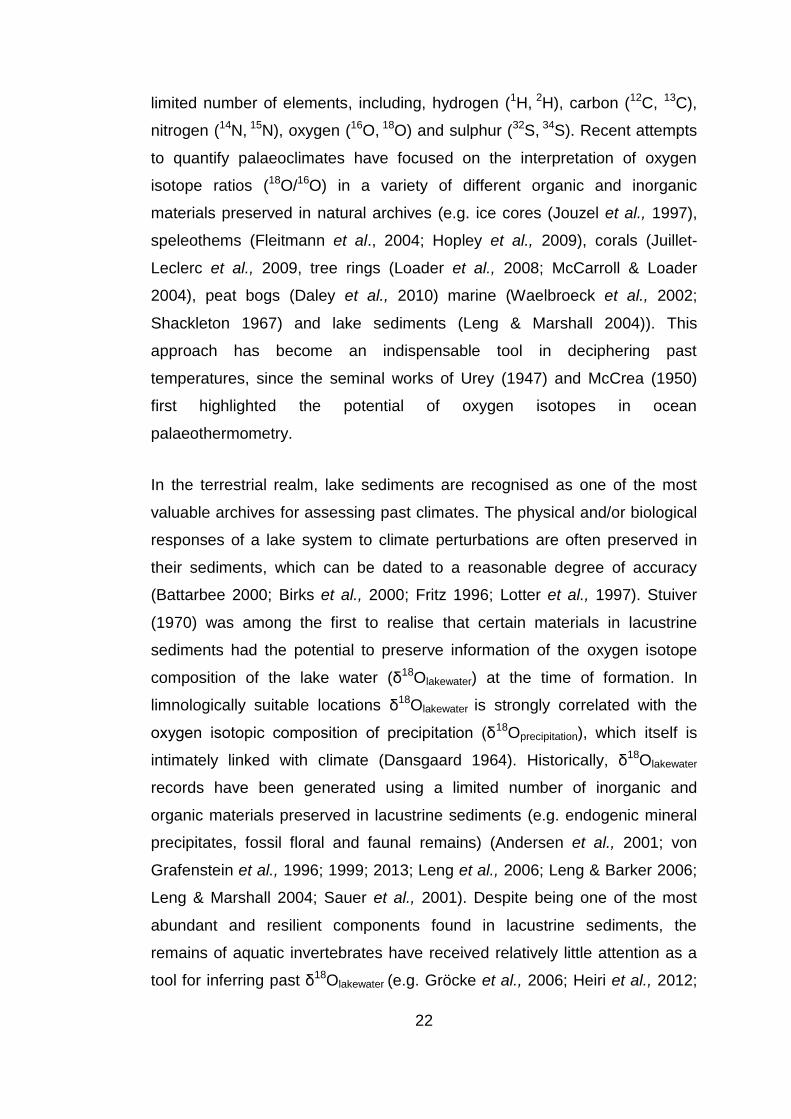
In cases of equilibrium precipitation, the oxygen isotope composition of
inorganic compounds (δ18Oinorganic) formed in a lake can be considered to
reflect δ18Olakewater modified by temperature-dependant isotope fractionations.
However, in practice the interpretation of δ18Oinorganic is complicated because
both δ18Olakewater and temperature are influenced by changes in climate (Leng
et al., 2006; Leng & Marshall 2004). Furthermore, disequilibrium effects may
cause disparities between the isotopic composition of the lake water and the
mineral precipitate (Figure 1-3) (see Leng et al., 2006; Leng & Marshall
2004).
36
Figure 1-3: Controls on the oxygen isotope composition of inorganic compounds (δ
18Oinorganic) preserved in lacustrine sediments. In cases of equilibrium, δ
18Oinorganic is
reflective of δ18
Olakewater modified by temperature-dependant fractionations and disequilibrium effects (Leng & Marshall 2004).
Organic compounds preserved in lacustrine sediments potentially offer a
more direct approach for inferring past δ18Olakewater, since they are anticipated
to be largely independent of kinetic (temperature related) and disequilibrium
effects (Leng et al., 2006). For example, δ18Oaquatic_cellulose records have been
used to infer past δ18Olakewater (e.g. Anderson et al., 2001; Edwards &
McAndrews 1989; Epstein et al., 1977; DeNiro & Epstein 1981; Sauer et al.,
2001; Wolfe et al., 2007). However, the reproducibility and reliability of
δ18Oaquatic_cellulose determinations can be compromised by the presence of
terrestrial cellulose, which is often enriched in 18O compared to aquatic
cellulose (Sauer et al., 2001). Supplementary elemental data can be used to
constrain the interpretation of cellulose sources, with low C/N ratios (<10)
interpreted to reflect predominantly aquatic derived organic matter (Wolfe et
al., 2001). However, Sauer et al. (2001) argued that elemental ratios are
insufficient criteria for interpreting the origin of cellulose.
Technical innovations in continuous flow stable isotope mass spectrometry
(e.g. Farquhar et al., 1997; Kornexl et al., 1999; Koziet 1997) have facilitated
the diversification and expansion of materials used for oxygen isotope
determinations. The chitinous remains of chironomid larvae (Insecta: Diptera:
δ18Oinorganic
37
Chironomidae) have recently received increasing attention as a δ18Olakewater
proxy (e.g. Heiri et al., 2012; Verbruggen et al., 2010; 2010b; 2011; Wang et
al., 2008; 2009; Wooller et al., 2004; 2008). This approach is underpinned by
the assumption that the oxygen isotope composition of chironomid remains
(δ18Ochironomid) is reflective of δ18Olakewater in which the larvae grew. Since
aquatic fauna primarily metabolise dissolved oxygen from their habitat water
and because isotopic exchange is thought to be negligible in these
exoskeletal fragments following biosynthesis, the remains of aquatic insects
are potentially capable of retaining information of their biochemical heritage
(Gröcke et al., 2006; Heiri et al., 2012; Miller 1991; Motz 2000; Nielson &
Bowen 2010; Schimmelmann 2010; Schimmelmann & DeNiro 1986;
Schimmelmann et al., 1986; Verbruggen et al., 2010a; 2010b; 2011 Wang et
al., 2009; Wooller et al., 2004; 2008). Furthermore, since chironomid remains
are easily identified under a light microscope the approach should be less
susceptible to contamination from semi-terrestrial/terrestrial taxa or
sedimentary components, which often have a deleterious influence on δ18O
determinations in other biomolecules. Consequently this approach is
potentially less technically challenging than oxygen isotope analysis in other
organic and inorganic compounds.
38
1.4 Chironomids in palaeoclimate reconstructions
This section will provide a brief introduction to chironomid biology and
ecology. This will be followed by a review of the development of oxygen
isotope analysis in chironomid remains. A comprehensive overview of the
application of stable isotopes (O, C, H and N) in chironomid remains can be
found in Heiri et al. (2012).
1.4.1 Biology and ecology
Chironomidae are a taxonomically diverse family of non-biting flies (Insecta:
Diptera) comprised of eleven subfamilies and estimated to contain ~15,000
species worldwide (Armitage et al., 1995). As larvae, chironomids are
ubiquitous in virtually all aquatic biomes, occupying an unparalleled number
of habitats (Brooks & Birks 2001; Brooks 2006; Ferrington 2008; Langdon et
al., 2004; Oliver 1971; Velle et al., 2005). The broad-scale distribution of
chironomids is restricted to a specific set of environmental conditions,
predominantly driven by temperature (Brooks 2000; Brooks et al., 2007;
Eggermont & Heiri 2012; Kurek 2008; Płóciennik et al., 2011; Self 2010;
Velle et al., 2005).
Chironomids are holometabolous (undergo metamorphism), developing from
an egg through four larval instar stages, the first three of which are restricted
to the aquatic realm, before emerging into the terrestrial realm as a winged
adult (Figure 1-4).
39
Figure 1-4: Schematic representation of the chironomid life cycle from Ruiz et al., (2006).
Each developmental stage of the chironomid life cycle will now be discussed
in more detail.
Egg stage- Eggs are laid (several hundred at a time) in a
hydrophilous gelatinous matrix directly into water or attached to a
suitable substrate. The gelatinous matrix offers protection and a
source of nourishment for the embryonic pro-larvae and the newly
hatched larvae (Oliver 1971).
Larval stage- This stage assumes a disproportionate importance in
the life cycle, relative to the other stages, encompassing four
progressively lengthening periods of growth, each defined by
exoskeletal ecdysis (periodic molting of the head capsule) (Walker
1987). The early instar stage is largely planktonic, permitting dispersal,
whereas the latter instars are generally sedentary.
Mature chironomid larvae can generally be described as having
elongate nine-segmented soft cylindrical bodies (2-30mm in length),
which bear a fully developed non-retractile, strongly sclerotized,
chitinous head capsule (Figure 1-5) (Brooks et al., 2007).
40
Figure 1-5: Schematic diagram of chironomid larvae (typically 2-30mm in length) showing key morphological characteristics from Epler (2001).
Larvae typically inhabit the uppermost sediments of both littoral and
profundal environments, within silken tubes constructed from
specialised organs (Brooks et al., 2007). Larvae may also be found
clinging on or burrowing into aquatic macrophytes, woody debris or
other invertebrates, as well as living freely within the water column
(Brooks et al., 2007; Bouchard & Ferrington 2008; Oliver 1971;
Płóciennik et al., 2011).
Pupal stage- This stage typically persists only a few hours or days
and involves the morphological rearrangement of larva in preparation
for adult emergence (Armitage et al., 1995; Oliver 1971). At maturity
pupa migrate to the water surface where the adult emerges into the
terrestrial realm, leaving the discarded pupal case on the surface of
the water (Bouchard & Ferrington 2008; Pinder 1986; Walker 1987).
Imago- The reproductive aspects of the life cycle are completed
during this stage (Oliver, 1971). Adult emergence within a population
is synchronised with changes in external stimuli (e.g. temperature and
photoperiod), which maximises copulation potential (Oliver 1971;
Pinder 1986). The adult stage persists anywhere between a few days
to a week (Oliver 1971; Pinder 1986).
41
The duration of the chironomid life cycle varies greatly among taxa, with
growth (i.e. the increase in larval body size) and development (i.e.
progression through the life cycle) predominately under the control of
temperature (Walker 1987). Laboratory rearing experiments have
demonstrated a strong positive correlation between chironomid development
and water temperature, up to a certain threshold (Ward & Cummins 1979).
Temperature may also have an indirect influence on chironomid growth and
development through the alteration of lake productivity, dissolved oxygen
concentration, thermal stratification, pH and salinity (Pinder 1986).
Chironomid larvae are generally found in lake sediments all year round. In
temperate climates chironomid adults typically emerge into the terrestrial
realm in spring or late summer, triggered by changes in water temperature
and light intensity (Johnson & Pejler 1987). The number of generations within
a population per year (voltinism) increases with MAT, with species from low
latitudes typically being multivoltine (multiple generations per year) whilst
those in temperate locations are most likely to be univoltine (single
generation per year) or bivoltine (two generation per year).
1.4.2 Chironomid-inferred temperature (CI-T) models
The chitinous head capsules of chironomid larvae, shed during ecdysis or
from deceased individuals, are often one of the most abundant macro-
invertebrate remains encountered in lacustrine sediments. These remains
are readily identifiable at least to a generic level, based on distinctive
morphological characteristics (Brooks et al., 2007). Since chironomids are
sensitive environmental indicators, fossil assemblages can be enumerated to
infer changes in past environmental conditions (e.g. Brooks & Birks 2001;
Brooks 2006; Langdon et al., 2004; Walker & Cwynar 2006).
Walker & Mathewes (1987) were among the first to suggest that mean July
air temperature was a dominant driver of the distribution of chironomid taxa.
This observation facilitated the development of chironomid-inferred
temperature (CI-T) models, to quantitatively infer past temperature from
42
stratigraphic changes in the taxonomic composition of chironomid
assemblages (e.g. Brooks & Birks 2001; Lotter et al., 1998; Walker et al.,
1991; Walker & Cwynar 2006; Walker & Mathewes 1987). CI-T models are
derived from regionally-calibrated training sets, which empirically link
contemporaneous taxonomic distributions and abundances to temperature
(Brooks & Birks 2001; Eggermont & Heiri 2012). CI-T models generally
produce estimates in accordance with other palaeoclimate reconstructions
(Brooks 2006; Eggermont & Heiri 2012; Heiri et al., 2007; Walker & Cwynar
2006) and instrumental records (Larocque & Hall 2003). However, disparities
have been observed due to difficulties in disentangling the response of
chironomid communities to changes in temperature (Bigler et al., 2002;
Brooks 2006; Brooks & Birks 2001; Eggermont & Heiri 2012; Velle et al.,
2010).
Although the broad-scale geographical distribution of chironomid taxa is
mainly driven by temperature, in-lake variables have also been observed to
influence chironomid distribution (Walker & Mathews 1989; Walker et al.,
1991). As a consequence chironomid assemblages can also be used to infer
past changes in pH (Henrikson et al., 1982), salinity (Eggermont et al., 2006),
water depth (Hofmann 1998; Korhola et al., 2000), hypolimnetic anoxia (Little
& Smol 2001; Quinlan et al., 1998) and trophic status associated with
changes in total phosphorous and chlorophyll-a (Brodersen & Lindegaard
1999; Brooks & Birks 2001; Lotter et al.,1998; Zhang et al., 2006).
43
1.4.3 Oxygen isotope analyses of chironomid head capsules: a tool in palaeoclimate reconstructions
In a pioneering study Wooller et al. (2004) demonstrated that the oxygen
isotope composition of chironomids (δ18Ochironomid), was highly correlated with
interpolated regional δ18Oprecipitation (r2= 0.96) from North American lakes
across a broad climatic range (Figure 1-6). However, this study was only
based on surface sediments collected from four lakes and no information
regarding δ18Olakewater was provided, making the assessment of oxygen
isotope fractionation between chironomid head capsules and lake water
(α18Ochironomid-lakewater) impossible. In a more extensive field-based study,
spanning 31 stratified lakes across Europe (41-69°N latitude), Verbruggen et
al. (2011) also observed robust linear relationships between δ18Ochironomid,
inferred δ18Oprecipitation (r2= 0.79) and δ18Olakewater (r
2 = 0.95).
Figure 1-6: Calibration of δ18
Ochironomid vs. inferred δ18
Oprecipitation, where the constant fractionation line (dashed line) displays a lower slope than the regression line (solid line). Assuming constant fractionation between chironomid head capsules and water, α = 1.028 (Wooller et al., 2004).
The authors of these studies speculated that; i) the remains of chironomid
larvae are in isotopic equilibrium with their habitat water and, ii) the imprinting
of the δ18Olakewater signal in chironomids is largely independent of temperature
dependant fractionations and vital effects. As a result they suggest
stratigraphic changes in δ18Ochironomid can be used to infer past δ18Olakewater
directly.
44
Wooller et al. (2004) were the first to infer past temperature changes from a
δ18Ochironomid record spanning the last 10,000 years. The results of this study
were largely in accordance with chironomid inferred summer water
temperature (SWT) and independent MAT records from the period (Wooller
et al., 2004). The same authors also produced another down-core record, in
which δ18Ochironomid variability was attributed to changes in the seasonality of
precipitation and the origin of air masses delivering precipitation to the study
area (Wooller et al., 2008).
Verbruggen et al. (2011) demonstrated that δ18Ochironomid successfully tracked
stratigraphic changes in δ18Obulk_carbonate from a Late-glacial sediment
sequence (Rotsee, Switzerland) (Figure 1-7). Therefore, δ18Ochironomid records
can compliment carbonate-derived δ18O records and provide an opportunity
to generate δ18O records from sites where carbonate sequences are absent
or incomplete. Furthermore, the coupling of organic and inorganic δ18O
archives from the same stratigraphic sequence offers a potentially powerful
quantitative approach for reconstructing past temperatures (e.g. Buhay et al.,
2012; Rozanski et al., 2010). This approach is underpinned by the
fundamental assumption that δ18Ochironomid is an uncorrupted proxy for
δ18Olakewater and that the two independent δ18O archives are formed
simultaneously from the same waters. Providing that δ18Olakewater can be
accurately inferred from δ18Ochironomid, calcification temperature can be
predicted based on the laws of thermodynamics.
45
Figure 1-7: Stable oxygen isotope record of bulk carbonate (left curve) and chironomids (right curve) from Late-glacial sediments Rotsee, Switzerland. Grey areas indicate cold periods (from Verbruggen et al., 2011). The chironomid remains were treated with 2M ammonium chloride (NH4Cl) to eliminate carbonate contamination.
Remaining challenges
In order for δ18Ochironomid to become a quantitative tool in the reconstruction of
past δ18Olakewater, and therefore past climates, the proxy needs to be
calibrated. Many aspects regarding the application and interpretation of this
proxy remain under developed. The most important remaining considerations
are: i) the development of standardised sample preparation and analytical
procedures, ii) rigorous calibration of the contemporary relationship between
δ18Ochironomid, δ18Olakewater and temperature to confirm the absence of
temperature dependant α18Ochironomid-H2O and iii) the development of
palaeotemperature estimates from δ18O measurements of co-existing
chironomid and carbonate samples. The absence of a standardised protocol
for the preparation of chironomid remains for δ18O analyses has restricted
the application of this approach. It is expected that once the methodology
has been developed and necessary calibration studies produced this
approach will increase in popularity (Heiri et al., 2012).
46
1.5 Project aims
This thesis aims to contribute to the on going development of δ18Ochironomid as
a tool for reconstructing past climates, with particular attention paid to:
a) The evaluation of molybdenum as an alternative to glassy-carbon
in high temperature pyrolysis reduction reactors during δ18O
analyses of organic compounds (Chapter 2).
b) Development of a standardised protocol for the preparation of
chironomid remains for δ18O analyses (Chapter 3).
c) Laboratory and field-based calibrations of the relationships
between δ18Ochironomid, δ18OH2O and temperature (Chapter 4).
d) The development of Late-glacial palaeotemperature
reconstruction based on stratigraphic changes in δ18Ochironomid
and δ18Obulk_carbonate (Chapter 5).
Specific objectives are developed in the individual chapters. The overall
findings and their implications are explored in the following chapters and
summarised in Chapter 6.
47
Chapter 2 Analytical developments: the search for improved precision of oxygen isotope determinations in oxygen-bearing organic compounds
2.1 Introduction
Effective and reliable continuous-flow oxygen isotope analyses from organic
compounds can be achieved through the coupling of a high temperature
pyrolysis unit (HTP) to a continuous flow isotope ratio mass spectrometer
(IRMS) (Figure 2-1).
Figure 2-1: Schematic representation of a high temperature pyrolysis (HTP) unit coupled to an IRMS (Gehre & Strauch 2003).
48
A prerequisite of HTP techniques is the quantitative thermal decomposition
(pyrolysis) of a sample into a single oxygen-bearing gas at temperatures in
excess of ~1200°C, with carbon monoxide (CO) being the thermodynamically
favoured product (Brand et al., 2009; Kornexl et al., 1999; Farquhar et al.,
1997; Gehre & Strauch 2003). Providing that the thermal decomposition of
the sample is quantitative, the CO gas produced can be considered to be
isotopically representative of the sample (Brenna et al., 1997). The thermal
decomposition of an organic compound can be described by the following
generalised formula:
O-Compound (solid) + C (solid) CO (gas) + Residues (solid, gas, liquid)
Following flash pyrolysis, the gaseous products (including H, N2 CO) are
swept through a isothermal gas chromatography column (5 Å molecular
sieve, 80-100 mesh), which separates the gases based on molecular mass
(Brand 1996; Koziet 1997; Werner & Brand 2001). A small proportion of the
gaseous transient is admitted to the IRMS, via an interface unit, where it is
ionized before being accelerated across an electrical potential gradient and
focused into a beam by a series of electrostatically charged lenses. The
positively charged ions present in the beam interact with a magnetic field in
the flight tube, with the flight path radii of individual atoms proportional to
their mass. Eventually these ions strike a series of collectors (Faraday Cups)
at the end of the flight tube, where individual ionic impacts are converted into
a voltage. The isotopic composition of the sample gas is determined by
monitoring the ion current intensities of relevant masses (i.e. m/z 28 and 30
for oxygen isotope determinations), with the relative differences between the
ion current ratios of the sample, reference material and calibrated reference
gases calculated on an internationally agreed scale (Gehre & Strauch 2003;
Hagopian & Jahren 2012; Werner & Brand 2001).
HTP systems typically utilise a tube-in-tube reduction reactor composed of a
glassy-carbon-lined alumina (Al2O3) column situated inside a vertical furnace,
held at temperatures in excess of 1200°C (Figure 2-2) (Accoe et al., 2008;
Gehre et al., 2004; Gehre & Strauch 2003; Koziet 1997; Werner 2003). The
49
reactor is partially filled with glassy carbon granules, which help prime
sample reduction, up to the hottest part of the reactor where a graphite
crucible is positioned (Boschetti & Iacumin 2005). The glassy carbon liner
provides an oxidation barrier between the gaseous pyrolytic products, the
granular glassy carbon bed and the Al2O3 tube, reducing the formation of
long-lived or permanent oxide complexes (Gygli 1993; Kornexl et al., 1999;
Werner & Brand 2001; Werner 2003).
Graphite Crucible
Figure 2-2: Schematic representation of a standard tube-in-tube pyrolysis reactor adopted in high temperature pyrolysis (HTP) units. Image modified from Kornexl et al. (1999).
Furnace
Glassy Carbon
Tube
Glassy Carbon
Granules
Alumina Tube
Silver Wool
Quartz Wool
Temperature
Sensor
50
However, glassy-carbon-lined HTP reduction reactors are commonly
associated with several problems: i) low/variable yields (i.e. non-quantitative
sample conversion into CO), ii) memory effects, iii) peak tailing as a result of
improper flushing of the gaseous pyrolytic products caused by the bypassing
of the carbon bed, and iv) high backgrounds arising from unwanted reactions
between the glassy carbon liner and the outer Al2O3 tube at elevated
temperatures (Lombino et al., 2012). These problems have a deleterious
influence on the analytical precision of δ18O determinations (Farquhar et al.,
1997; Kornexl et al., 1999; Lombino et al., 2012).
51
2.2 δ18O analysis of organic compounds: problems with pyrolysis in molybdenum-lined reactors1
In an attempt to improve the analytical precision associated with δ18Oorganic
measurements the performance of a molybdenum (Mo)-lined reduction
reactor was evaluated. In this section a modified version of a manuscript
published in the Journal Rapid Communications in Mass Spectrometry
(Lombino et al., 2012; see appendix A-I for full manuscript), evaluating the
performance of a Mo-lined reduction reactor during δ18Oorganic determinations,
will be presented. The manuscript was produced in collaboration with Prof.
Tim Atkinson (Department of Earth Sciences, University College London)
and Dr. Steve Firth (Department of Chemistry, University College London),
who both provided analytical support and guidance during the production of
this article. This investigation was undertaken at University College London’s
Bloomsbury Environment Isotope Facility (BEIF), using a high temperature
conversion elemental analyser (TC/EA), coupled via a ConFlo III open split
interface to a DeltaXP IRMS (all units from ThermoFisher Scientific, Bremen,
Germany).
2.2.1 Reactor configuration and testing
The tested reduction reactor was composed of an Al2O3 tube (internal
diameter 13mm; outer diameter 17mm; length 470mm) lined with 0.1mm
thick Mo-foil (99.95% purity) (supplied by SerCon, Crewe, UK). The reactor
was partially filled with a 60mm deep bed of coarse (3-4mm) glassy carbon
granules, supported within the hottest zone of the reactor by a folded Mo-
plug (Figure 2-3a).
The configuration of the Mo-reactor was constrained by the construction of
the TC/EA furnace, resulting in significant differences from the reactor
employed in Stuart-Williams et al. (2008). The most striking difference being
the broadness of the relative hot-zones, as shown in Figure 2-3b, and a
wider Al2O3 tube (i.d. 16mm). Based on the available information it was
1 Published as: Lombino et al., 2012
52
inferred that the glassy carbon bed in Stuart-Williams et al. (2008) was
approximately twice as deep as the one tested in this pilot (~110–120mm).
Stable isotope determinations were conducted on silver encased aliquots
(150μg ± 10μg) of two internationally distributed reference materials, IAEA
601 (δ18OV-SMOW: +23.3‰), IAEA 602 (δ18OV-SMOW: +71.4‰) (International
Atomic Energy Agency, Vienna, Austria) and a benzoic acid laboratory
standard (Benzoesäure; Hekatek HE 33822501). The majority of analyses
during performance testing were conducted at 1400°C, however furnace
temperatures were systematically varied (1350-1430°C) independently to He
carrier gas flow rate (60 to 90 mLmin−1) in search of improved precision.
53
Figure 2-3: (a) Construction of the Mo-lined reactor for the TC/EA system. (b) Comparison between the temperature profiles and glassy carbon bed thickness for the TC/EA and the Mo-lined reactor used by Stuart-Williams et al. (2008). The vertical scales are offset so that the tops of the glassy carbon beds are aligned. Zones of corrosion damage in TC/EA reactor shown on the left (Lombino et al., 2012).
54
2.2.2 Reactor performance
Stuart-Williams et al. (2008) reported that the typical analytical precision
associated with δ18Oorganic determinations using Mo-lined reactors was
<0.25‰ (1σ). However, the reproducibility of δ18O determinations in this
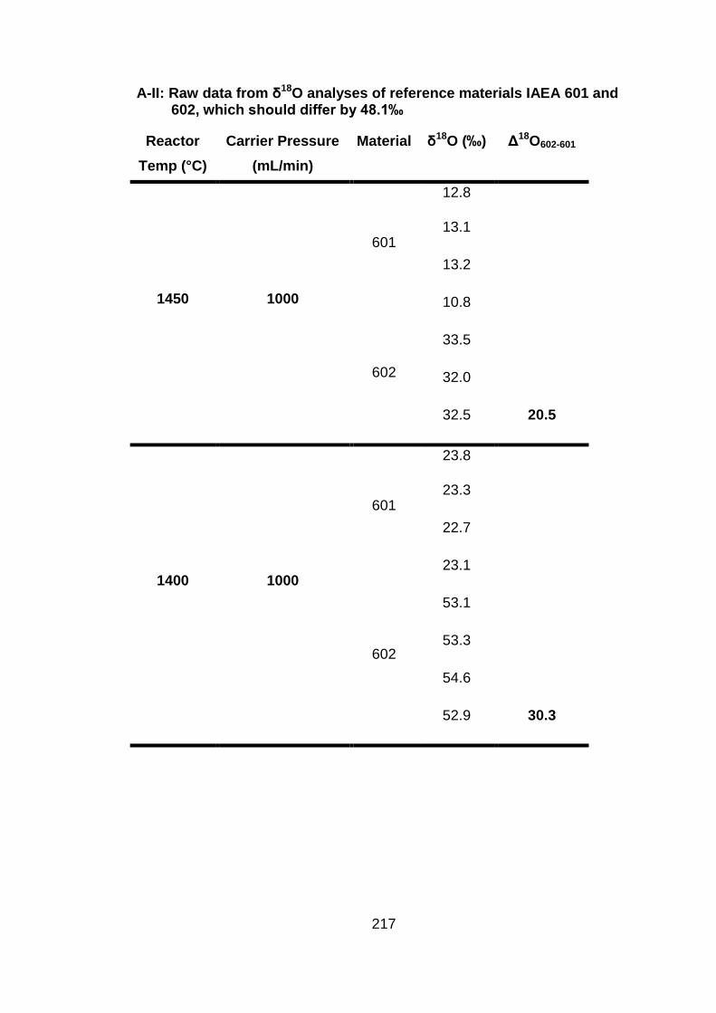
investigation was between 0.4-3‰ (1σ). Moreover, δ18O determinations
were associated with severe scale compression of up to 20‰ during
memory trials conducted at 1400°C, but under varying carrier gas flow
rates (60 to 90 mLmin−1) (see Appendix A-II). CO yield per unit weight of
carbon in benzoic acid was also observed to be variable under different
constant flow rate regimes (Figure 2-4).
Figure 2-4: Variability of CO gas yield with carrier gas flow rate and inferred residence time in contact with glassy carbon at temperatures in excess of 1100°C. Histogram show grouped data from individual analyses; square symbols show mean for each flow rate plotted against inferred residence time (Lombino et al., 2012).
60 ml/min
75 ml/min
90 ml/min
55
The apparent isotope fractionation in the modified reactor indicates that
quantitative reduction of sample O into CO was not achieved in the
tested system. Non-quantitative sample reduction can either be due to
incomplete pyrolysis or the partitioning of oxygen into phases other than
gaseous CO. Given the relative chemical simplicity of benzoic acid and
the high reactor temperatures, incomplete pyrolysis appears unlikely.
Sample reduction to CO2 could potentially account for the partitioning of
oxygen, however its absence from the gases emerging from the reactor
indicated that the partitioning was most likely to have been into a non-
gaseous phase. In order to investigate this hypothesis the elemental
composition of sections from two used Mo-lined reactors were analysed
by scanning electron microscopy energy-dispersive X-ray spectroscopy
(SEM-EDX) (Goldstein et al., 1992) and Raman spectroscopy (Gilson &
Hendra 1970).
2.2.3 Examination and analysis of used reactors
Two used reactors were gently broken open using a hammer. The Mo-
liners had become brittle and were severely corroded and pitted,
particularly in the hottest part of the furnace. Based on visual
examination both liners displayed similar characteristic zonation. The
elemental compositions of each of these zones are described below
(Figure 2-5a)
Zone I- spanned the upper 130mm of the Mo-liner. Temperatures
in this part of the reactor ranged from 450-1150°C (Figure 2-3b).
The Mo in the zone had a violet/brown lustre, consistent with
MoO2 (Cotton & Wilkinson 1966; Heslop & Jones 1976; Partington
1958; Sidwick 1950) (Figure 2-5a). No SEM-EDAX or Ramen
spectroscopy data is available from this section.
Zone II- spanned approximately 40mm. The zone was
characterised by a bronze/gold patina (Figure 2-5a), which gave
way to a band of bright metal. The metal band corresponds to the
region just above the carbon bed. EDX spectra from the inner
56
surface of the Mo-liner indicates the presence of elemental Mo (30
atom%) and O (69 atom%), similar proportional contributions plus
trace amounts of Al characterise the outer surface of the Mo-liner
as well.
Globular residues found adhering to the inner surface of the Mo-
liner in the lower section of this zone were composed of Ag
(90 atom%) and elemental C (10 atom%) (Figure 2-5b), these
must have originated from the splashing of molten silver during
pyrolysis.
Zone III- spanned approximately 25mm and corresponds with the
upper part of the carbon bed where temperatures were >1350°C
(Figure 2-3b). The Mo-liner in this zone showed extensive pitting
and dulling with surface encrustations both on inner and outer
surfaces (Figure 2-5a). Encrustations found on the inner surface of
the Mo-liner were mainly comprised of elemental Mo (85 atom%)
and O (15 atom%). EDX spectra of encrustations found on the
outer surface of the Mo-liner indicate the presence of elemental O
(58 atom%), Al (29 atom%), N (10 atom%) and Mo (2 atom%)
(Figure 2-5c).
The inner surface of the Al2O3 tube was stained black in this zone
and extended into Zone IV, above and below this deposit the
Al2O3 retained its original white colour. Raman spectroscopy
showed the presence of graphitic carbon within these black
deposits.
Zone IV- spans the lower 35mm of the carbon bed, where
temperatures exceed 1100°C (Figure 2-3b). The inner surface of
the Mo-liner was dulled and covered by metallic globules (Figure
2-5a), up to several mm in diameter, composed of Ag (51 atom%)
along with substantial proportions of elemental C (32 atom%), and
O (15 atom%) (Figure 2-5d).
57
Zone V- spans the cooler (400 – 1100°C) region below the Mo-
plug (Figure 2-3b). Both inner and outer Mo-liner surfaces carried
a patina of Mo-oxides (Mo: 41 atom%, O: ~ 52 atom%) on which
fine closely spaced hemispherical globules composed of Ag (77
atom%) and elemental C (19 atom%) were deposited (Figure
2-5e). Increased fining and density of the globules could be
observed with increasing distance.
58
Figure 2-5: A) Photograph of used Mo-liner. (B) SEM image and EDX analysis of inner liner surface from Zone II, showing silver globule (spectrum 1) adhering to mosaic-like patina of Mo-oxides (spectra 2 and 3). (C) SEM image and EDX analyses of outer liner surface from Zone III, showing areas of light-coloured Mo metal (spectrum 1) and darker patina containing Al and Mo oxides and a nitrogen-bearing phase (spectrum 3). (D) SEM image and EDX analyses of the inner surface from Zone IV, showing cracked patina of Mo-oxide (spectrum 1), plus 2 mm diameter blob of silver containing carbon and oxygen (spectrum 2). (E) SEM image and EDX analyses of inner liner surface from Zone V with ~0.1mm globules of silver containing carbon (spectrum 2) on a patina of Mo-oxide. Spectrum 1 contains both components (Lombino et al., 2012).
59
2.2.4 Discussion
Mo-oxide patinas were ubiquitous throughout the length of the tested Mo-
lined reactors. There are three potential sources of oxygen within the
reactor: a) diffusion of atmospheric oxygen through the Al2O3 tube at
elevated temperatures, b) self-diffusion of oxygen from the Al2O3 or direct
interactions between the Al2O3 tube and Mo at elevated temperatures or,
c) oxygen-bearing gaseous products of pyrolysis. Extensive patination
and corrosion observed on the inner surface of the Mo-liners is
suggestive that the genesis of the oxygen, within our system, is likely to
have originated from within the reactor. The other two potential sources
of oxygen (a and b) are likely to have also contributed to the formation of
Mo-oxides and corrosion of the Mo-liner, to some degree. For example,
the presence of nitrogen on the outer surface of the Mo-liner in Zone III
(Figure 2-5c) is suggestive of the diffusion of air through the Al2O3 tube.
The oxygen bearing products produced during the pyrolysis of benzoic
acid could include CO, CO2 and H2O, however the latter two will be
reduced to CO in the presence of excess carbon at elevated
temperatures. Consequentially, CO and H2 are the principal gases
expected inside the Mo-liner, along with the He carrier gas. Mo metal is
known to react with gaseous CO to produce Mo-oxides and carbon
(Reaction I below) (Sidwick 1950). The principal oxides of Mo are MoO2
and MoO3. The melting points (MP) and boiling points (BP) of these
oxides are far lower than the expected maximum temperatures in the
heart of the reactor (MoO2 MP 782°C, BP 1257°C; MoO3 MP 795°C, BP
1155°C; see Cotton & Wilkinson 1966; Heslop & Jones 1976; Partington
1958; Sidgwick 1950), consequently these oxides could theoretically
exist in their vaporised form within the hot zone of the reactor,
condensing to form patinas in the cooler parts. The consumption of
oxygen during the formation of MoO can potentially explain the observed
variability in CO yields per unit weight of carbon (Figure 2-4) and will
directly contribute to isotopic fractionation of the remaining CO. This
fractionation is unlikely to have been the sole cause of the scale
60
compression observed in our system, as this would require the degree of
fractionation to vary systematically with sample δ18O. An alternative
scenario could be isotopic exchange between gaseous CO and Mo-oxide
reservoirs that have accumulated over time in the reactor. The other
principal gas present in the reactor is H2, which is known to react with
MoO2 at temperatures in excess of 500°C to form Mo-metal and water
(Cotton & Wilkinson 1966; Holleman & Wiberg 2001) (Reaction II). At
temperatures in excess of 1000°C the water produced during pyrolysis
will be partially reduced on glassy carbon, re-forming as H2 and CO
(Reaction III). Thus Mo and C in the reactor will take part in a circular
series of reactions with the gases present:
I. (m x n)CO + nMo → nMoOm + (m x n)C (Sidwick 1950)
II. pMoOm + (m x p)H2 → pMo + (m x p)H2O
III. (m x p)H2O + (m x p)C → (m x p)H2 + (m x p)CO.
Reaction I will sequester a portion of the oxygen in the original CO into
Mo-oxides. Reaction II followed by III will return some of this oxygen as
CO. This back conversion will only be complete if n=p in the above
scheme, and also that Reaction III runs to completion. If both criteria are
met, the Mo-liner will be corroded, but would not be associated with any
Mo-oxide patinas. The presence of MoO patinas throughout the length of
both studied Mo-liners strongly suggests that the return of gaseous CO is
incomplete in this case (p<n). In standard HTP reduction reactors (Figure
2-2), reaction III only runs to completion in temperatures in excess of
1350 – 1400°C (Gehre et al., 2004; Gehre & Strauch 2003), with
catalysis by Ni being required at lower temperatures. This suggests that
there is scope for additional isotopic fractionation of the final CO leaving
the reactor, through kinetic effects in both Reactions II and III. It is
61
speculated that the varying scale compressions observed in δ18O of the
final CO may be a function of differential fractionations between Reaction
I and Reactions II and III, as well as the degree of inequality p<n and
other possible factors. The latter include the possibility that Reactions II
and III take place over a range of temperatures as the gases stream
downwards from the hottest zone into cooler regions and Mo-oxides
condense from the vapour to the liquid and solid phases. Once the Mo-
liner has been pierced by corrosion due to Reaction I, as seems to have
occurred quite quickly in this pilot, some of the gases and vapours may
migrate down the annulus between the Mo-liner and the outer Al2O3 tube,
where there is no access to solid carbon apart from that produced by
Reaction I. The presence of graphitic carbon on the inner surface of the
Al2O3 tube in the hottest part of the reactor supports the occurrence of
this reaction. As a consequence of the migration of these gases into the
annulus the majority of water produced in Reaction II will not be
converted back in CO and H2. In the core of the reactor, where carbon is
abundant, Reaction III can be expected to run to completion in Zone III
where the local temperature is high enough, but may not do so in the
cooler lower part of the carbon bed (Zone IV), and cannot do so where
carbon is absent (Zone V). The yield of CO gas, its isotopic composition
and resultant scale compression, are likely to depend upon the interplay
of reaction rates, local temperatures, carrier gas flow rates and the
residence times of the gases in the parts of the reactor that are most
favourable for Reactions II and III. The condition of the reactor liner,
especially whether it is pierced by corrosion, and the amount of Mo-oxide
deposit that has built up over time are further factors. The Mo-oxide
deposit is a potential locus for Reaction II, so the fractionation it causes
in the final output of CO may depend on the whole history of reactor use
and the δ18O values of the samples that have been analysed previously,
as there will be a memory of these in the Mo-oxide δ18O.
If the scheme of reactions envisaged is correct, then successful, accurate
analysis of organic compounds using Mo-lined reduction reactors would
62
require conditions such that Reactions II and III can return all oxygen to
gaseous CO, so that Mo-oxides would not build up in the reactor. This is
most likely to be achieved if the sample gases have a long residence
time in contact with carbon in the hottest part of the reactor, optimising
recovery of oxygen to CO via Reaction III. Such conditions appear to
have been met in the HTP system utilised by Stuart-Williams et al.
(2008), who managed to achieve excellent precision without scale
compression using this approach. As can be seen from Figure 2-3b the
reactor used by Stuart-Williams et al. (2008) had a broader hot-zone and
larger diameter than the reactor tested in this pilot. Rough estimations,
based on figures provided by Stuart-Williams et al. (2008), suggests that
if volumetric gas flows were equal in the two systems, the gas residence
time in the hottest part of Stuart-Williams’ reactor was 2-3 times greater
than the configuration tested in this study. Therefore, it is hypothesised
that residence time of gas in contact with carbon at ~1400°C is critical to
the performance of the Mo-lined reduction reactors.
A possible line of development for HTP units, which have a narrow hot-
zone (Figure 2-3b), might be to inactivate the Mo surface of the liner. Mo
is known to form a variety of carbides by reaction with CO (Gillet et al.,
1976) and a coating of these might inhibit the corrosion reactions with the
metal. Borda (1985) describes the use of Mo-carbide-coated carbon as a
catalyst for the conversion of oxygen in organic compounds into CO at
1080°C. Inactivation might also slow down corrosion of the outside
surface of the Mo-liner by oxygen diffusion through the alumina tube or
by direct reaction with the Al2O3. Direct measurement of air diffusion
through the alumina tubes under operating temperatures would also help
to establish the relative importance of these sources of oxygen in causing
the corrosion observed in this study.
63
2.2.5 Conclusion
No previously published studies have investigated the chemical
composition of HTP reactors after use. Mo-liners are relatively
inexpensive and easy to fabricate but they are apparently unsuitable for
use in the TC/EA system in the configuration tested by this study. The
principal reason for this appears to be the production and build-up of Mo-
oxides as a patina or coating on the liner as a result of the reaction
between Mo-metal and CO gas, causing poor precision and variable CO
yields. To some extent the loss of CO is compensated for by reactions
between Mo-oxides and hydrogen gas derived from the sample,
producing water, followed by reduction of the water to CO and H2 by
reaction with glassy carbon. However, these restoring reactions probably
introduce further fractionation effects and may be responsible for scale
compression observed in testing. Despite all this, it is possible to obtain a
precision of <0.25‰ during δ18O analyses using Mo-liners, as
demonstrated by Stuart-Williams et al. (2008). From comparison of
reactor designs, it is concluded that the depth of the hot zone and the
time that the pyrolysis products spend within it are critical factors,
although diffusion of atmospheric oxygen through the walls of the
alumina tubes may also contribute. Analysts intending to develop a Mo-
lined HTP system should ensure that their furnace and reactor design
follow those of Stuart-Williams et al. (2008) and provide a residence time
at ~1400°C for the produced gases of at least 4 seconds. The
approximate residence times in the system tested in this pilot varied from
~1.3 to ~2 seconds, which was not sufficient to promote quantitative
conversion of oxygen from the sample into CO. Although Mo-lined
reactors have potential for δ18O determinations within some HTP
systems, it is clear that the chemistry of reactions is not straightforward.
64
2.3 Oxygen isotope determinations of chironomid head capsules
Following the negative experiences with Mo-lined reduction reactors and
time constraints, this line of method development was abandoned in
favour of standard HTP techniques. Although the search for improved
analytical precision ultimately proved fruitless, it did provide a valuable
opportunity to become intimately associated with analytical procedures.
All oxygen isotope analyses of chironomid remains were performed at
Durham University’s Stable Isotope Biogeochemistry Laboratory (SIBL),
using a TC/EA coupled to a Delta V Advantage IRMS, via a ConFlo III
open split interface (all units from ThermoFisher Scientific). The TC/EA
was equipped with a zero-blank auto-sampler (Costech International,
Milan, Italy) and an integrated GC column (5 Å molecular sieve), which
was held at 60°C to maximise chromatographic separation. All analyses
were performed without dilution, due to limited sample sizes.
2.3.1 Reproducibility and calibration
All results presented in this thesis are normalised to the V-SMOW scale
by calibration against three international reference materials IAEA 600,
601 and 602 (measured vs. expected r2 >0.99), which were monitored
regularly throughout each sample run. The isotopic values of the chosen
standards bracketed the expected sample range. For each standard,
average measured values and standard deviations are shown in Table
2-1.
65
Table 2-1: Measured values and 1σ for the international reference materials together with their published values. All values are presented in ‰ vs. the V-SMOW scale.
Published δ18O Measured δ18O n
IAEA 600 −3.5 −2.5 ±0.64 60
IAEA 601 +23.3 +25.8 ± 0.40 60
IAEA 602 +71.4 +71.8 ± 0.59 60
The precision of δ18O analyses in this investigation was between ±0.40-
0.64‰ (1σ), based on repeated analysis of reference materials. Unless
otherwise stated this range is used as an estimate of analytical
uncertainty throughout this thesis.
66
Chapter 3 Methodological development: the evaluation of optimal sample size and the geochemical influence of chemical pre-treatments on chironomid head capsules
The reproducibility and reliability of δ18O determinations from insect
cuticles can be compromised by compositional heterogeneity
(Schimmelmann 2010; Schimmelmann & DeNiro 1986) and exogenous
contamination (Verbruggen et al., 2010a). Since HTP techniques are
largely indiscriminate, resulting in the conversion of all oxygen bearing
organic compounds present within a sample into CO gas during
pyrolysis, sample heterogeneity can alter the original δ18O values
masking climate-driven changes (see Section 2.1) (Gehre & Strauch
2003; Verbruggen et al., 2010a; 2011). In order to produce meaningful
δ18O measurements, efforts should be made to limit the abundance of
non-amino-polysaccharide impurities present within a sample. Strategies
employed to reduce sample heterogeneity should maintain the isotopic
integrity of the original sample or introduce a systematic offset that can
be corrected for (Nielson & Bowen 2010; Schimmelmann 2010).
67
3.1.1 Chapter Aims and Objectives
This chapter aims to develop a standardised protocol for the preparation
of sub-fossil, fossil and contemporary chironomid remains for δ18O
analysis. This will be achieved by: -
Ascertaining optimal sample size required for reproducible
δ18Ochironomid analyses.
Systematically investigating the geochemical influences
associated with different reagent types, concentration, reaction
temperature and exposure duration.
68
3.2 Sample size analysis
Prior to evaluating the geochemical influences of chemical pre-
treatments on chironomid remains, the optimal sample size required for
reproducible δ18Ochironomid measurements needs to be established. The
amount of sample required for online δ18O analysis varies depending on
the measured substrate and instrument sensitivity (Hagopian & Jahren
2012; Heiri et al., 2012). The isolation of chironomid head capsules from
lacustrine sediments is often the most time consuming step in
chironomid-based studies, as a result the establishment of the optimal
weight required for reproducible δ18Ochironomid analyses was one of the
most important steps during the early stages of this project.
Sample size requirements were assessed through the repeated (x3)
analyses of chironomid head capsules across a range of different
weights (10-100µg) (Figure 3-1). For this purpose, chironomid head
capsules were manually isolated from commercially sourced whole
freeze-dried Chironomus riparius larvae (King British, UK). Based on
communication with the supplier it was assumed that these larvae were
subjected to similar conditions during growth. Digestive tracts and muscle
tissue were carefully detached from the head capsules using a scalpel, to
avoid contamination by organic material potentially present in the larval
gut. Samples ranging from 10-100µg (±2µg) were weighed out into silver
capsules (6 x 4mm, Elemental Microanalysis) and analysed.
69
Figure 3-1: δ18
O values of chironomid head capsules isolated from commercially grown Chironomus riparius larvae (King British, UK) plotted against sample weight (see appendix B-I for raw data). Error bars represent 1σ (0.8 - 0.5) in each weight. Dashed line represents the optimal sample weight required for reproducible analyses.
A minimum sample size of >20μg was required to produce reproducible
δ18Ochironomid measurements, based on analyses with no sample dilution
(Figure 3-1; see appendix B-I for raw data). However, given the scatter
observed in δ18Ochironomid across the different weights (1σ = 0.8-0.5‰) it
was decided that a minimum weight of 60 ±10μg would be used
throughout this investigation. Chironomid head capsules vary greatly in
size and weight depending on species and developmental stage making
the estimation of a minimum number of fossil head capsules necessary
for an individual measurement difficult (Heiri et al., 2012); based on
experiences throughout this investigation between 10-50 head capsules
are necessary to achieve the desired weight.
22
23
24
25
26
27
28
0 20 40 60 80 100
δ18O
(‰
V-S
MO
W)
Weight (μg)
70
3.3 An introduction to chitin
In order to provide adequate context for the remainder of this chapter a
brief introduction into chitin will now follow.
3.3.1 Chemical structure of chitin
Chitin is a linear amino-polysaccharide composed of N-acetyl-β-D-
glucosamine (2-acetamido-2-deoxy-β-D-glucose) monomers held
together by β- (14)-glycosidic linkages (Figure 3-2) (Acosta et al.,
1993; Abdullin et al., 2008; Das & Ganesh 2010; Majtán et al., 2007;
Percot et al., 2003a; 2003b). The idealised chemical structure of chitin is
rarely found in nature, with its stoichiometric formula variable between
two end-members; fully acetylated chitin (C8H13O5N) and the partially de-
acetylated derivative chitosan (C6H11O4N) (Gröcke et al., 2006).
Figure 3-2: Theoretical molecular structure of chitin (C8H13O5N) (Gröcke et al., 2006).
Chitin bears a strong chemical resemblance to cellulose, differing only in
the substitution of a hydroxyl group at the C-2 position with an acetamido
group (Acosta et al., 1993; Cohen 1987; 2001; Das & Ganesh 2010;
Dutta et al., 2002; 2004; Einbu 2007; Gröcke et al., 2006; Hogenkamp
2006; Kurita 2006; Merzendorfer & Zimoch 2003; Ravi-Kumar 1999;
Schimmelmann 2010; Zhang et al., 2000).
71
Chitin exhibits a highly ordered, crystalline structure and can be found in
nature in three polymorphic forms (α-chitin, β-chitin and γ-chitin; see
Figure 3-3). Each of these polymorphs have unique physical properties
owing to differences in the degree of hydration, crystal cell size, number
of chitin chains per unit cell and structural arrangement of chitin chains
(Acosta et al., 1993; Einbu 2007; Kramer & Koga 1986; Nation 2008).
Figure 3-3: Polymorphic forms of chitin found in nature (α-chitin, β-chitin and γ-chitin). Adjacent chitin chains in the α-and β-forms are arranged in an antiparallel and parallel manner respectively, while every third chain has the opposite orientation to the two preceding chains in the γ-form (Carlström 1957; Einbu 2007; Hogenkamp 2006; Merzendorfer 2006; Merzendorfer & Zimoch 2003).
The antiparallel arrangement of chitin molecules in the α-form permits
tight packaging of chitin chains to form microfibrils (Merzendorfer &
Zimoch 2003; Nation 2008). α-chitin is commonly found in structures
where extreme mechanical strength and stability is required (e.g.
exoskeletons) (Einbu 2007; Rinaudo 2006). In contrast chitin chains in β
and γ-forms are less tightly packed and subsequently contain fewer intra-
and inter-chain hydrogen bonds (Merzendorfer & Zimoch 2003). The
reduced packing tightness and increased degree of hydration in these
polymorphs improves the flexibility of the chitinous structure (e.g. in
insect cocoons) (Einbu 2007; Hogenkamp 2006; Merzendorfer & Zimoch
2003; Rinaudo 2006).
72
3.3.2 Chitin in nature
Chitin is one of the most abundant amino-polysaccharides in the
biosphere and forms an essential extracellular structural component in a
wide variety of invertebrate groups (e.g. Arachnida, Arthropoda,
Brachiopoda, Mollusca) (Andersen 1979; Aranaz et al., 2009; Cohen
1987; 2001; Hogenkamp 2006; Majtán et al., 2007; Merzendorfer 2006;
Merzendorfer & Zimoch 2003; Miller 1991). Chitin is particularly
conspicuous in insect cuticles, where it accounts for ~10-50% of the
overall biomass (Acosta et al., 1993; Andersen 1979; Kurita 2006; Majtán
et al., 2007; Zhang et al., 2000). Insect cuticles are complex composite
structures, composed of three main layers (Figure 3-4) (Andersen 1979;
Barbakadze et al., 2006; Nation 2008; Neville 1975):
Figure 3-4: Cross-section of typical multi-layered insect cuticle (Barbakadze et al., 2006).
Epidermal cells- These cells are responsible for the secretion of
chitin, protein and some lipids under hormonal control during cuticle
synthesis (Nation 2008).
Procuticle (divided into the exocuticle and endocuticle)- This
layer is composed of successive lamella (or sheets) of chitin
microfibrils/rods embedded within a largely proteinaceous matrix, in a
similar arrangement to steel re-enforced concrete (Figure 3-5) (Einbu
2007; Nation 2008).
Epicuticle- The impermeable non-chitnous outmost layer of an insect
cuticle.
73
Figure 3-5: Diagram of chitin rod set within a protein matrix in insect cuticle (Nation 2008).
The structural rigidity of insect cuticles is enhanced through cross-linking
(sclerotization) of protein and chitin moieties, via extensive covalent
bonding between the amine and carbonyl groups of adjacent chitin
chains, as well as cross-linking with phenol and quinone compounds
(e.g. catecholamines and histidine moieties) (Figure 3-6) (Einbu 2007;
Hopkins & Kramer 1992; Merzendorfer & Zimoch 2003; Nation 2008).
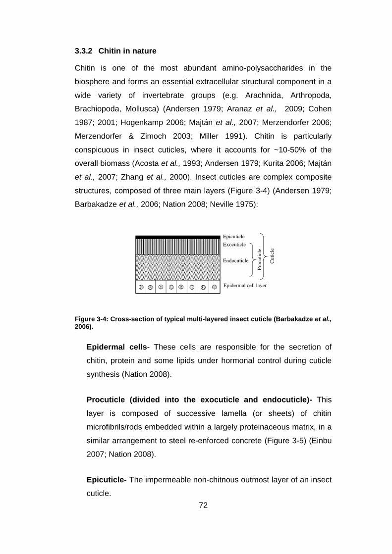
The chemical composition and degree of sclerotization of insect cuticles
varies greatly among different species and even within different
developmental stages (Nation 2008). For an extensive review of
sclerotization in insects see Hopkins and Kramer (1992).
Figure 3-6: Chemical structure of chitin linked to proteins in insect cuticles through catecholamines and histidine moieties (Verbruggen et al., 2010a).
74
3.3.3 Chitin biosynthesis in insects
Insect cuticles have a limited capacity to keep pace with growth,
consequently insects must periodically shed their cuticles (ecdysis)
(Merzendorfer & Zimoch 2003; Nation 2008). Although chitin is one of the
most abundant biopolymers on the planet the biosynthesis of chitin
remains poorly defined (Merzendorfer 2006). Chitin biosynthesis appears
to follow an orderly sequence of multifaceted, interconnected,
intracellular and extracellular reactions (Figure 3-7) (Cohen 1987; 2001).
The process is initiated by the cytoplasmic biotransformation of simple
metabolites (e.g. glucose, fructose, glucosamine, trehalose) into the
substrate uridine diphospho-N-acetyl-glucosamine (UDP-GlcNAc), which
is used in the polymerisation of N-acetyl-β-D-glucosamine monomers in a
reaction catalysed by the membrane-integral enzyme chitin synthase
(Andersen 1979; Cohen 1987; 2001; Merzendorfer & Zimoch 2003;
Merzendorfer 2006). Nascent chitin polymers (α, β or γ-chitin) are
extruded into the extracellular space where they spontaneously undergo
crystallisation, forming chitin microfibrils of varying length and diameter
(Andersen 1979; Cohen 1987; 2001; Merzendorfer & Zimoch 2003;
Nation 2008).
75
Figure 3-7: Anticipated chemical pathway of chitin biosynthesis in insects (Merzendorfer & Zimoch 2003).
76
3.4 Preparation of chironomid remains for δ18O analysis
The use of chitin monomer units, such as D-glucosamine hydrochloride
(GlcN.HCl), as a substrate for stable isotope analyses can potentially
circumvent the inherent issues associated with the analysis of insect
cuticles (Schimmelmann & DeNiro 1986; Schimmelmann et al., 1986). In
brief, the preparation of GlcN.HCl involves the hydrolysis of mineral and
proteinaceous moieties using HCl and NaOH, followed by ion-exchange
chromatography purification (Schimmelmann 2010). However, the
preparation of GlcN.HCl is labour-intensive and results in the addition of
one oxygen atom, originating from water, to each GlcN.HCl molecule
(Schimmelmann 2010). Furthermore, the preparation of GlcN.HCl is
associated with substantial sample weight loss (> 95%) precluding the
use of this substrate where samples are limited (Hodgins et al., 2001;
Motz 2000; Tripp et al., 2004).
Alternatively, since chitin is largely insoluble in most organic solvents,
non-amino-polysaccharide impurities present within a sample (both
compositional and exogenous) can be largely decomposed via a series
of liquid solvent-based extractions, yielding a residual chitin rich “isolate”
(Schimmelmann 2010). Although the purified residual will invariably
contain some covalently-bound impurities, it should represent a more
suitable substrate for stable isotope analysis compared to chitinous
biomass (Nielson & Bowen 2010; Schimmelmann 2010).
The purification of insect cuticles typically involves three main stages,
broadly categorised as:
Decolouration- The elimination of waxes, oils, pigments and
resins present within the epicuticle. This is typically achieved
using an organic solvent solution such as dichloromethane:
methanol (DCM: MeOH).
77
Demineralisation- The elimination of acid-soluble moieties
(e.g. catechols or carbonate in the case of crustaceans) present
within the cuticle (Zhang et al., 2000) and exogenous
contamination (e.g. endogenic carbonates). HCl is the preferred
reagent and is typically applied at a concentration of between
0.25 and 2M for 1-48 hours at temperatures varying from 0 to
100°C (Charoenvuttitham et al., 2006; Einbu 2007; Percot et
al., 2003a, 2003b; Zhang et al., 2000).
Deproteination - The elimination of base-soluble moieties (e.g.
proteins) present within the cuticle. NaOH is the preferred
reagent for deproteinisation and is applied at a concentration of
1M for 1-72 hours at temperatures ranging from 50-100°C
(Einbu 2007; Percot et al., 2003a, 2003b). Complete hydrolysis
can only be achieved through more aggressive treatments (e.g.
5% NaOH at 100°C) (Brine & Austin 1981; Kurita 2006; Nation
2008).
A similar multi-stage chemical pre-treatment was successfully adopted by
Nielson & Bowen (2010) to limit non-amino-polysaccharide impurities in
Artemia franciscana prior to δ18O analyses (see Nielson & Bowen 2010).
However, previous studies have demonstrated that great care is required
during the preparation of chironomid remains for δ18O analyses.
Verbruggen et al. (2010a) reported that alkaline- (10% KOH, 2 hours,
20°C; 28% KOH, 24 hours, 70°C) and acid-based (30% HCl, 1 hour, 40%
HF, 2 hours, 20°C) chemical pre-treatments induce significant alterations
in chironomid head capsule geochemistry and morphology (Figure 3-8).
Consequently the authors of this study recommended that chemical pre-
treatments should be avoided altogether during the preparation of
chironomid head capsules for δ18O analysis (Verbruggen et al., 2010a).
However, in a more recent publication the same authors recognised the
importance of eliminating exogenous contamination in order to produce
reliable δ18Ochironomid measurements (Verbruggen et al., 2011).
78
Figure 3-8: Effects of different chemical pre-treatments on the δ18
O of head capsules of Chironomus riparius larvae. Values are plotted as deviations from reference treatment (10% KOH, 1 hour, 70°C). Note that ASE+LD treatment refers to a chemical pre-treatment commonly employed for the purification of cellulose, involving accelerated solvent extraction (ASE) and successive treatment with sodium chlorite and glacial acetic. Image from Heiri et al. (2012) originally adapted from Verbruggen et al. (2010a).
3.4.1 Materials and methods
In this investigation the geochemical influence associated with reagents
used during decolouration (DCM: MeOH), demineralisation (HCl) and
deproteination (NaOH) were evaluated using an isotopically well-
characterised, purified shrimp chitin standard (δ18O = +27.9 ±0.3‰;
Sigma-Aldrich, C9752, St. Louis, MO, USA) and a chironomid standard,
consisting of head capsules isolated from commercially sourced freeze-
dried larvae grown under the same conditions (see Section 3.2). The
efficiency of each purification stage is known to be a function of reaction
conditions (Abdullin et al., 2008; Charoenvuttitham et al., 2006; Percot et
al., 2003a, 2003b), therefore reagent concentration (0.25M and 1M),
reaction duration (1 and 24 hours) and temperature (20°C and 70°C)
were varied systematically in order to optimise reaction conditions (Table
3-1). Sub-samples were exposed to MiliQ water (δ18O V-SMOW = −6.9‰) to
represent chemically untreated samples for comparison.
79
Sample aliquots (1000-2000μg) were exposed to the relevant chemical
solutions (1ml) in sealed 1.5ml plastic Eppendorf tubes, which were left in
either a water bath set at 20°C or in an oven set at 70°C, for 1 or 24
hours. Following chemical exposure for the desired period, samples were
centrifuged, at 12000 r.p.m for 10 minutes, and the reagent solution
pipetted off. The samples were then repeatedly (x3) rinsed with MiliQ
water, before being freeze-dried for 5 days. Residual material from each
experiment was re-weighed, to calculate the weight loss associated with
each treatment. The pre-treated samples then underwent δ18O analysis
at SIBL, Durham University, using standard HTP techniques (see Section
2.1), to establish the isotopic differences between untreated and treated
samples (Δ18Ountreated-treated). It should be noted that no attempts were
made to determine the effectiveness of each treatment at removing
different moieties present in the cuticle. The experiment was not
replicated due to time constraints, however replicate δ18O analyses were
performed for each of the tested conditions where sufficient material was
available.
80
Table 3-1: Matrix of different pre-treatments tested in this investigation.
Treatment
Concentration Temperature
(°C)
(°
Duration
(hours)
2:1 0.25M 1M 20 70 1 24
DCM: MeOH X X X X X X
X X X
x x X
HCl N/A
X X X X X X
X X X
X X X
X X X
X X X
X X X
X X X
NaOH N/A
X X X X X X
X X X
X X X
X X X
X X X
X X X
X X X
DCM: MeOH +
HCl + NaOH
X X X X X X X X
X X X X
X X X X
X X X X
X X X X
X X X X
X X X X
Control N/A X X X X
X X
X X
81
3.5 Results and discussion
3.5.1 Sample weight loss
The average weight loss associated with each of the purification stages
is presented in Table 3-2 for both sample materials. It should be noted
that some of the weight loss observed in each experiment is likely to
have been attributed to sample loss during solution pipetting and
weighing. An average sample weight loss of ~40% was observed in
control treatments for both sample materials, which was used as an
estimate of error introduced during sample preparation. Assuming that
this error was systematic, several semi-quantitative conclusions can be
drawn from the average weight loss data.
The average weight loss associated with each purification stage is
virtually indistinguishable from the control treatment for purified chitin
standard (Table 3-2). In contrast, the average weight loss observed in
contemporary chironomid head capsules varied across the different
purification procedures. For example, exposure to DCM: MeOH
treatments resulted in an average weight loss of ~60%, while the NaOH
treatments were associated with an average weight loss of ~80% (Table
3-2). Based on these results it can be inferred that DCM: MeOH-soluble
moieties (e.g. lipids, waxes and/or pigments) and NaOH-soluble moieties
(e.g. proteins) form a significant component in contemporary chironomid
head capsules. These findings are consistent with Verbruggen et al.
(2010a), who reported near equal proportions of chitin and protein
derived moieties in sub-fossil chironomid head capsules. Average weight
loss associated with HCl-based treatments was virtually indistinguishable
from the control treatments, indicating that acid soluble moieties form a
relatively minor component in both materials.
82
Table 3-2: Average weight loss and δ18
O data associated with each of the tested pre- treatments (see appendix B-II for raw data).
Chitin Powder Chironomid Head Capsules
Treatment Average Weight
Loss (%) δ
18O 1σ
Average Δ
18Ountreated-
treated
Average Weight
Loss (%) δ
18O 1σ
Average Δ
18Ountreated-
treated
DCM:MeOH 42 +28.5 0.3 −0.6 58 +14.1 1.5 0.4
HCl 48 +28.9 0.1 −1.0 42 +15.4 1.1 −1.0
NaOH 38 +28.7 0.4 −0.8 83 +17.6 2.2 −3.2
DCM:MeOH + HCl + NaOH
50 +28.8 0.7 −0.9 86 +15.9 1.6 −1.5
Control 40 +27.9 0.3 46 +14.5 0.9
83
3.5.2 Chemical treatment impact on δ18O
The geochemical influence associated with each of the purification stages
tested in this investigation is presented in Figure 3-9 as an average deviation
of treated samples from untreated samples (∆18Ountreated-treated).
Figure 3-9: a) Average ∆18
Ountreated-treated observed in chitin standard and b) contemporary head capsules. Error bars represent 1σ across the treatments tested in each purification stage. It should be noted that no statistical analysis could be performed to assess the relationships between the different treatments as the data was drawn from a non-homogenous data set (i.e. each symbol represents an average from all of the tested conditions).
84
∆18Ountreated-treated for each individual tested reaction condition is presented in
Figure 3-10.
-9
-7
-5
-3
-1
1
3Δ
δ18O
un
treate
d-t
reate
d (‰
V-S
MO
W)
a)
-9
-7
-5
-3
-1
1
3
Δδ
18O
un
treate
d-t
reate
d (‰
V-S
MO
W)
b)
Figure 3-10: a) ∆18
Ountreated-treated for each of the tested reaction conditions for chitin standard and b) chironomid remains. White symbols represent 1 hour treatments; black symbols represent 24 hour treatments. Black cross- 24 hour, 20°C; black star- 24 hour, 70°C; white cross- 1 hour, 20°C; white star- 1 hour, 70°C, square- 0.25M, 20°C; circle- 0.25M, 70°C; diamond- 1M, 20°C; triangle- 1M, 70°C. Each symbol represents average value for treatment type where repeat measurements were possible. Error bars represent 1σ of replicated analysis.
DCM:MeOH HCl
NaOH
DCM;MeOH +
HCl+ NaOH
85
The following section describes the effects of each of the tested pre-
treatments on δ18O vales in both sample materials.
DCM: MeOH
The tested DCM: MeOH-based treatments were on average associated with
a ∆18Ountreated-treated of ~ −0.6‰ and ~ +0.4‰ for the chitin standard and
contemporary head capsules respectively (Table 3-2). The offsets observed
in both sample materials are largely indistinguishable from analytical error
(±0.30-0.45‰) and 1σ of δ18O measurements in the respective control
groups.
The tested DCM: MeOH treatments were observed to introduce variability in
δ18O determinations of contemporary head capsules (1σ = 1.5‰). The
average ∆18Ountreated-treated was +1.9 ±0.4‰ in contemporary head capsules
exposed to hot (70°C), prolonged (24 hours) DCM: MeOH treatment;
whereas the average ∆18Ountreated-treated was −1.5‰ in contemporary head
capsules exposed to cold (20°C), short (1 hour) treatments (Figure 3-10).
Considering the relatively high average sample weight loss (see Table 3-2), a
potential mechanism responsible for creating the observed isotopic variability
is the selective removal of 18O enriched solvent-soluble moieties.
HCl
The tested HCl-based treatments were associated with an average
∆18Ountreated-treated of ~ +1.0‰ in both sample materials, although analysis of
the chitin standard exposed to the most extreme reaction conditions (1M, 24
hours, 70°C) was not possible due to excessive sample loss. Extensive acid
hydrolysis at elevated temperatures is known to catalyse de-acetylation
(cleaving of the glycosidic bonds between chitin monomer units) producing
chitosan, which is soluble in acidic aqueous solutions (Acosta et al., 1993;
Aranaz et al., 2009; Das & Ganesh 2010; Einbu 2007; Hodgins et al., 2001;
Nielson & Bowen 2010; Schimmelmann 2010; Tripp et al., 2004; Verbruggen
et al., 2010a).
86
The similarity in the magnitude of the offsets observed in both sample
materials indicates that isotope exchange is likely to be the primary
mechanism for the observed variability in δ18O measurements, since acid
soluble moieties should not be present in the purified chitin standard. The
lowering of sample pH is known to promote isotope exchange between the
‘freely exchangeable’ oxygen atoms within the acetyl group and/or the
hydroxyl oxygen bound to the glucose ring in organic matter, with the OH’
group in the water used to dilute the acid (Hodgins et al., 2001; Nielson &
Bowen 2010; Schimmelmann 2010; Verbruggen et al., 2010a). The relative
proportion of freely exchangeable and non-exchangeable O-atoms will differ
among different types of organic molecules. Chemical attack by H+ will alter
the macromolecular structure of organic molecules releasing oxygen-bearing
fragments, increasing potential sites for isotope exchange. This process may
be selective to a degree and is apparently strongly correlated with reaction
conditions (Figure 3-10).
NaOH
The NaOH treatments tested in this investigation were associated with an
average ∆18Ountreated-treated of ~ −0.8‰ and ~ −3.2‰ for the chitin standard and
contemporary head capsules respectively (Table 3-2). Once again the offset
observed in the chitin standard is largely indistinguishable from analytical
error (±0.30-0.45‰) and 1σ of δ18O measurements in the control group. In
contrast the offset observed in contemporary head capsules is much larger.
The primary mechanism responsible for creating variability in δ18O
determinations of chironomid head capsules is likely to be the selective
removal of base soluble moieties (e.g. mainly proteins), which appear to be
isotopically lighter than the residual bulk material. Prolonged exposure to
concentrated NaOH treatment at elevated temperatures is associated with a
∆18Ountreated-treated of ~ −8.0‰. A similar magnitude of offset was observed in
Verbruggen et al. (2010a) in chironomid remains exposed to ‘harsh’ basic
treatments (e.g. 28% KOH for 24 hours at 100°C) (see Figure 3-8). However,
NaOH treatments are associated with high average sample weight loss of up
87
to ~ 90% in contemporary remains exposed to ‘harsh’ reaction conditions.
Therefore, a balance must be struck between the complete elimination of
base soluble moieties and the preservation of sufficient samples to perform
δ18O analyses.
DCM: MeOH+ HCl+ NaOH
Samples subjected to each of the purification stages were on average
associated with a ∆18Ountreated-treated of ~ −0.9‰ and ~ −1.5‰ for the chitin
standard and contemporary head capsules respectively. In contrast to the
chitin standard, the ∆18Ountreated-treated in contemporary head capsules is
greater than the analytical error (±0.30-0.45‰) and 1σ of δ18O
measurements in the control group (see Table 3-2). The magnitude of
∆18Ountreated-treated in contemporary head capsules is about half the sum of the
offsets observed in each individual treatment as outlined above.
88
3.6 Standardisation of the preparation of chironomid head capsules for δ18O analysis
The results presented in this investigation demonstrate that each of the
tested purification stages are sensitive to reaction conditions, with harsh (e.g.
1M, 24 hours, 70°C) conditions likely to provoke the removal of soluble
moieties, a degree of isotope exchange and/or chitin de-acetylation. Isotope
exchange will result in the overprinting of the original oxygen isotope ratios,
leading to spurious palaeoclimate interpretations. In order to limit these
detrimental effects reagent concentration (2:1 or 0.25M), exposure duration
(24 hours) and reaction temperature (20°C) were standardised. The
standardisation of reaction conditions significantly reduced δ18O variability
observed in the chitin standard (standardised 1σ = 0.4; unstandardised 1σ =
0.7) and the chironomid head capsules (standardised 1σ = 0.7;
unstandardised 1σ = 1.6). The average Δ18Ountreated-treated for the chitin
standard and contemporary head capsules exposed to the standardised pre-
treatment is presented in Figure 3-11.
Figure 3-11: Plot of average Δ18
Ountreated-treated for chitin standard (diamond) and head capsule standard (square) subjected to the chosen standardised chemical pre-treatment (sequential soaking in 2:1 DCM: MeOH, 0.25M HCl, 0.25M NaOH solutions for 24 hours at 20°C). Error bars represent 1σ of replicated analysis (n = 6 for both materials). Dashed line represents average repeated control δ
18O measurement.
-2.5
-2.0
-1.5
-1.0
-0.5
0.0
0.5
Δδ
18O
un
treate
d-t
reate
d (‰
V-S
MO
W)
Chitin Standard Contempoary HeadsContemporary Heads Contemporary Heads
89
The average Δ18Ountreated-treated in the chitin standard exposed to the
standardised pre-treatment was −0.9‰ (n=6), which encompasses both
analytical and preparatory uncertainties. Isotope exchange is likely to be the
primary mechanism responsible for creating this offset, given that extensive
de-acetylation is not evident and that the original material contains few
compositional impurities (pers.comm.Sigma-Aldrich; 20 August 2013).
Consequently, one may conclude that the standardised pre-treatment
procedure is associated with ~ −0.9‰ offset. The average Δ18Ountreated-treated
of contemporary head capsules exposed to the standardised pre-treatment
was −1.4‰ (n=6). Since ~ −0.9‰ of this offset is likely to have been due to
isotope exchange, the remaining ~ −0.6‰ offset can be considered to be
caused by the selective removal of impurities, most likely compositional in
the instance of contemporary remains tested in this investigation. δ18O
determinations of samples treated using a standardised multi-stage
procedure were statistically different from untreated samples in both tested
sample materials (p < 0.01). Consequently it may be necessary to apply a
+0.9‰ correction during δ18O analyses of samples treated using this
procedure.
The current absence of a standardised protocol for the preparation of
chironomid remains for δ18O analyses has restricted the application of
δ18Ochironomid in palaeoclimate reconstructions and hindered inter-laboratory
comparisons (Wang et al., 2008; Verbruggen et al., 2010a). It is hoped that
the procedure described in this chapter can form the basis for the
standardisation of preparatory procedures in future δ18Ochirononmid analysis.
However, additional systematic studies are required in order to fully assess
the effectiveness of the adopted procedure at limiting non-amino
polysaccharide impurities by comparing chemical composition of the
standard materials before and after treatment (e.g. pyrolysis-GC/MS
analysis), while studies are also required to assess the influence of different
types of exogenous contamination (e.g. carbonate and silicate) on
δ18Ochironomid determinations.
90
Chapter 4 Towards a mechanistic understanding of the incorporation of oxygen isotopes in chironomid head capsules: laboratory and field-based calibration of δ18Ochironomid, δ
18Olakewater and temperature.
4.1 Overview
In order for δ18Ochironomid to become a quantitative tool for reconstructing past
δ18Olakewater and, indirectly past climates, it is first necessary to refine our
understanding of the inherent fractionations associated with the incorporation
of environmental isotopic signatures into chironomid head capsules. Oxygen
isotope fractionations between chironomid head capsules and habitat water
(α18Ochironomid-H2O) are poorly defined. In their pioneering study, Wooller et al.
(2004) concluded that α18Ochironomid-H2O was constant and largely
indistinguishable from oxygen isotope fractionation in aquatic cellulose
(α18Oaquatic cellulose-H2O = 1.025-1.028) (e.g. Edwards & McAndrews 1989; Wolfe
et al., 2001). The apparent similarity between α18Ochironomid-H2O and α18Oaquatic
cellulose-H2O suggests that common biochemical reactions are likely to govern
fractionation in both organic compounds. Since α18Oaquatic cellulose-H2O is largely
independent of kinetic (temperature related) and disequilibrium effects, one
may assume that the same is true for chironomids, based on the findings
presented in Wooller et al. (2004). Although it should be noted that Wooller et
al. (2004) did not account for secondary effects associated with atmospheric
circulation patterns, hydrological conditions and catchment characteristics,
which can alter δ18Oprecipitation during transportation to the lake or while in the
lake (see Sections 1.3.2 and 1.3.3). Consequently their assessments require
experimental verification.
In this chapter the relationship between δ18Ochironomid, habitat water δ18O and
temperature was evaluated in a series of laboratory and field-based
calibration studies, with these results forming the foundations for the
interpretation of stratigraphic changes in δ18Ochironomid (Chapter 5).
91
4.1.1 Chapter aims and objectives
This chapter aims to improve the mechanistic understanding of the
incorporation of oxygen isotopes in chironomid head capsules and refine the
characterisation of the relationship between δ18Ochironomid, δ18Olakewater and
temperature in contemporary chironomid remains. This will be achieved by: -
Accurately measuring α18Ochironomid-H2O as a function of temperature in
a series of controlled laboratory experiments (Section 4.2).
Investigating the relationship between δ18Ochironomid and δ18Olakewater in
a spring-fed pond, known to be subjected to negligible temporal
variations in water chemistry and δ18Olakewater (Section 4.3).
Investigating δ18Ochironomid in a series of lakes that experience seasonal
variations in δ18Olakewater, water chemistry and temperature (Section
4.4).
The calibration of relationships between δ18Ochironomid, δ18Olakewater and
temperature in contemporary settings is fundamental to the development of
this approach as a tool in palaeoclimate reconstructions.
92
4.2 An in vitro assessment of the influence of temperature on oxygen isotope fractionation between chironomid head capsules and water
4.2.1 Rearing experiments
Laboratory studies are an excellent model for examining the influence of
different parameters on the stable isotopic composition of a compound
(Gannes et al., 1997). In this investigation, Chironomus riparius larvae were
reared from eggs (supplied by Huntington Life Sciences Ltd) in glass
Erlenmeyer flasks, containing 2 litres of bottled mineral water and 500g of
sand (combusted at 550°C for six hours to eliminate extraneous food
sources). The flasks were situated inside isothermal cabinets (Natural History
Museum, London) set at different constant temperatures (5, 10, 15, 20, 25°C)
(Figure 4-1). Replicate experiments at each of the test temperatures were
conducted concurrently in the same isothermal cabinet to minimise
temperature variations between replicate experiments.
Figure 4-1: Erlenmeyer flasks located inside an isothermal cabinet (NHM, London).
The flasks were kept in complete darkness to prohibit photosynthetic activity
and were loosely sealed with aluminium foil to limit evaporation. Each flask
was typically provided with 1.5ml suspension of finely ground Tetramin fish
food flakes, every other day. The food suspension was made weekly, by
blending 4g of fish food flakes with one litre of water. Rationing was adjusted
!
93
according to water quality and larval behaviour as the decomposition of
uneaten food can lead to increased microbial activity and reduced dissolved
oxygen concentration, which may hinder larval development. Since no
aeration could be provided to the flasks inside the isothermal cabinets, water
quality was maintained through regular partial water replacements. One litre
of water was siphoned off each flask weekly and replaced with stock mineral
water stored at the relevant temperature, to ensure satisfactory dissolved
oxygen concentration and maintain optimal environmental conditions for
growth and development.
Experiments were terminated once the majority of larvae had reached the
final instar stages, with experiment duration varying depending on larval
growth rates.
94
4.2.2 Sampling
Water samples- Water samples were taken regularly throughout the
experiments to track changes in δ18O. Samples were filtered using
disposable cellulose acetate filters (0.2μm pore size) and were stored at 4°C,
in 5ml screw top glass vials with no headspace.
Stable isotope analyses of water samples were undertaken at the 'Lifer'
stable isotope laboratory, Department of Earth, Ocean and Ecological
Sciences, University of Liverpool. Oxygen (18O/16O) and hydrogen (D/1H)
isotope ratios were determined simultaneously using a Picarro WS-CRDS
system, with the results presented in this thesis being the average of at least
8 sequential injections of 2μl of water. Results were normalised onto the V-
SMOW scale using internationally distributed standards. Internal precision
was < 0.08‰ for δ18O and < 0.4‰ for δD measurements.
Water Chemistry- Camlab Handylab 1 battery powered hand-held meters
attached to a data logger were used to measure electrical conductivity
(μScm−1), dissolved oxygen concentration (mgL−1) and pH of the growth
water in each experiment, at near weekly intervals. The meters were
calibrated before use in accordance with manufacturer’s procedures. It
should be noted that water chemistry measurements were performed prior to
the partial water replacements.
Tinytalk (TK-0040) data loggers were used to monitor water temperature at
hourly intervals in one of the flasks in each of the isothermal cabinets, due to
an insufficient number of loggers. However, it is assumed that temperature
variations between flasks in the same cabinet were negligible.
Chironomid Larvae- The contents of each flask were washed through a
1mm mesh sieve and chironomid larvae were isolated from the retained
residue, using fine tipped forceps. The larvae were frozen whole, with
freezing assumed to have no influence on δ18Ochironomid (Verbruggen et al.,
2010a).
95
Following defrosting, head capsules were manually isolated from larval
bodies under a stereo-microscope (x25 magnification) using a mounted
needle and fine tipped forceps. Care was taken to remove as much of the
digestive tract and muscle tissue as possible from the head capsules, which
then underwent chemical pretreatment following the procedures outlined in
Section 3.6, prior to δ18O analysis (Section 2.3).
96
4.2.3 Results and Discussion
Temperature, chemistry and δ18O of the growth water
The maintenance of constant conditions during this investigation proved
problematic, particularly at higher temperatures where the oxygen demands
of the chironomid larvae were increased due to enhanced metabolic activity.
A summary of mean water chemistry (pH, dissolved oxygen concentration
and electrical conductivity), temperature and δ18OH2O from each experiment
is provided in Table 4-1.
Table 4-1: Mean δ18
O, pH, dissolved oxygen concentration and electrical conductivity in each of the rearing experiments. Temperature measurements were not taken from replicate flasks due an insufficient number of data loggers. An additional flask was reared at 15°C during a preliminary study.
Temperature
(°C)
δ18OH2O
(‰ V-SMOW) pH
Dissolved
Oxygen
(mgL−1)
Electrical
Conductivity
(μScm−1)
5.6 ± 0.4 −7.4 ± 0.18 7.2 ± 0.2 7.3 ± 1.5 230 ± 12
−7.5 ± 0.12 7.3 ± 0.1 7.2 ± 1.4 237 ± 10
10.5 ± 0.4 −7.6 ±0.18 7.4 ± 0.2 7.1 ± 1.3 256 ± 18
−7.5 ±0.21 7.2 ± 0.2 7.2 ± 1.4 259 ± 25
15.2 ± 0.4 −7.3 ±0.07 7.4 ± 0.2 6.7 ± 1.9 247 ± 18
−7.4 ±0.11 7.3 ± 0.2 6.2 ± 2.3 259 ± 14
−7.5 ±0.15 7.3 ± 0.1 6.4 ± 1.9 259 ± 16
20.2 ± 0.3 −7.3 ±0.16 7.6 ± 0.1 6.8 ± 1.0 250 ± 7
−7.3 ±0.14 7.6 ± 0.0 6.8 ± 1.1 252 ± 8
24.9 ± 0.5 −7.3 ±0.25 7.5 ± 0.2 6.1 ± 1.8 292 ± 17
The evolution of water chemistry, temperature and δ18OH2O throughout the
duration of each experiment is presented in Figure 4-2.
99
-8.0
-7.8
-7.6
-7.4
-7.2
δ18O
H2O
(‰
V-S
MO
W)
9.5
10.0
10.5
11.0
11.5
Tem
pe
ratu
re (
°C)
200
210
220
230
240
250
260
270
280
290
300
Co
nd
uctv
itiy
(µ
Scm
-1)
0
1
2
3
4
5
6
7
8
9
10
Dis
so
lved
Oxyg
en
(m
gL
-1)
7.0
7.2
7.4
7.6
7.8
0 10 20 30 40 50 60 70 80 90 100 110
pH
Day
c)
10°C
106
Figure 4-2: a-j evolution of water chemistry and stable isotope data throughout the duration of each experiment. ‘ and “ denote replicate cultures.
j) 25°C
107
Since no significant mortality events were observed throughout the duration
of this investigation, conditions are assumed to have remained within the
ecological tolerances of the Chironomus riparius larvae; however it should be
noted that eggs failed to hatch in one of the cultures at 25°C. Water
temperature (1σ = ±0.3 - 0.5°C), pH (1σ = ±0.1 - 0.2), and δ18OH2O (1σ = ±0.1
- 0.3‰) remained essentially constant in each experiment, although limited
evaporative enrichment was apparent in nearly all of the flasks (Figure 4-2).
The observed variability in δ18OH2O (1σ ±0.1 - 0.3‰) in this investigation is
considerably lower than the variation reported in a similar controlled
laboratory study, in which δ18OH2O varied by 1.1 to 1.8‰ (1σ) in experiments
that ran for ~8 weeks (Wang et al., 2009). Dissolved oxygen concentration
fluctuated in each experiment, which is likely to have been associated with
changes in the metabolic processes (e.g. respiration) in the chironomid
larvae and the decomposition of uneaten food.
Experiment duration
Temperature has a profound influence on chironomid physiology, with the
duration of each experiment varying at different temperatures. Larval
development was slowest in experiments conducted at 5°C and fastest at
25°C. A summary of the time for Chironomus riparius larvae to reach the 4th
instar stage is provided in Table 4-2.
Table 4-2: Chironomus riparius larvae development time (from eggs to 4th
instar stage) at different constant temperatures.
Temperature (°C)
Larval Development Time (Days)
5 130
10 110
15 90
20 70
25 50
108
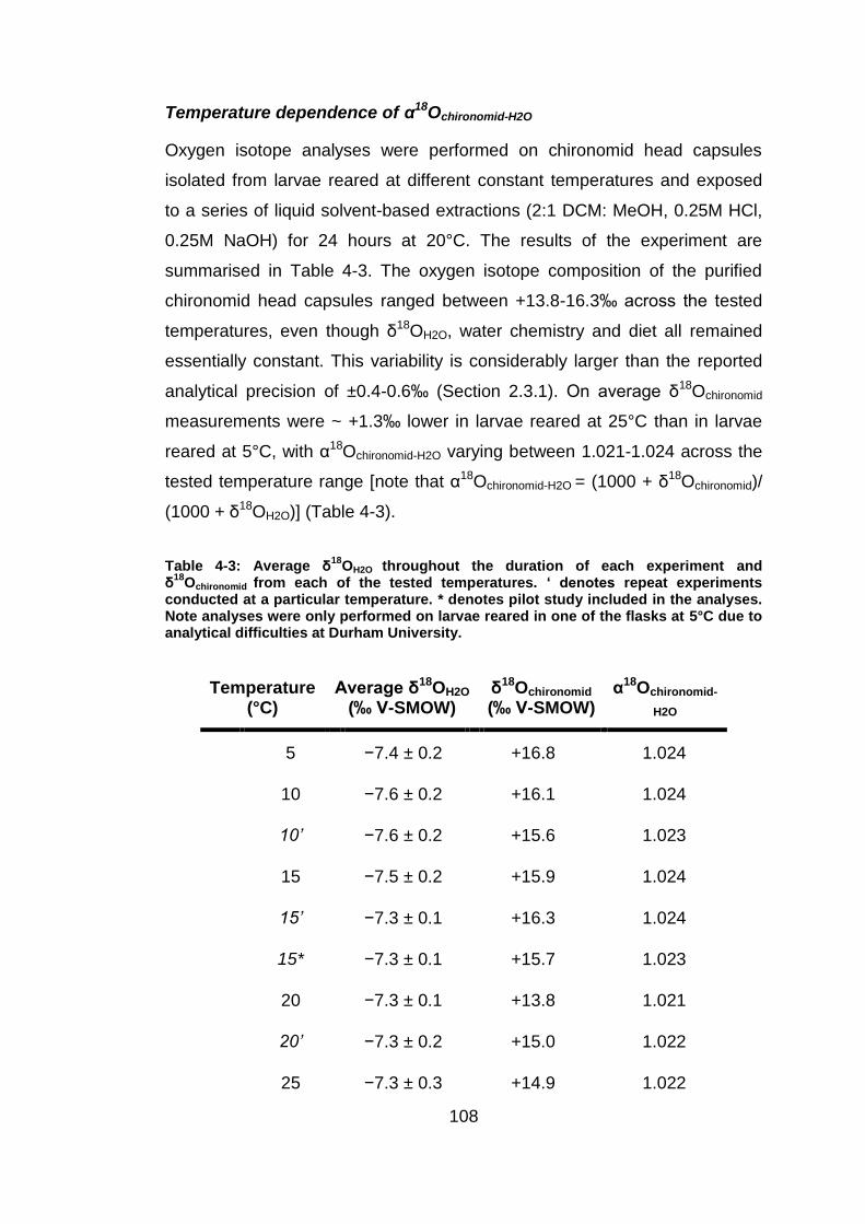
Temperature dependence of α18Ochironomid-H2O
Oxygen isotope analyses were performed on chironomid head capsules
isolated from larvae reared at different constant temperatures and exposed
to a series of liquid solvent-based extractions (2:1 DCM: MeOH, 0.25M HCl,
0.25M NaOH) for 24 hours at 20°C. The results of the experiment are
summarised in Table 4-3. The oxygen isotope composition of the purified
chironomid head capsules ranged between +13.8-16.3‰ across the tested
temperatures, even though δ18OH2O, water chemistry and diet all remained
essentially constant. This variability is considerably larger than the reported
analytical precision of ±0.4-0.6‰ (Section 2.3.1). On average δ18Ochironomid
measurements were ~ +1.3‰ lower in larvae reared at 25°C than in larvae
reared at 5°C, with α18Ochironomid-H2O varying between 1.021-1.024 across the
tested temperature range [note that α18Ochironomid-H2O = (1000 + δ18Ochironomid)/
(1000 + δ18OH2O)] (Table 4-3).
Table 4-3: Average δ18
OH2O throughout the duration of each experiment and δ
18Ochironomid from each of the tested temperatures. ‘ denotes repeat experiments
conducted at a particular temperature. * denotes pilot study included in the analyses. Note analyses were only performed on larvae reared in one of the flasks at 5°C due to analytical difficulties at Durham University.
Temperature (°C)
Average δ18OH2O
(‰ V-SMOW)
δ18Ochironomid
(‰ V-SMOW) α18Ochironomid-
H2O
5 −7.4 ± 0.2 +16.8 1.024
10 −7.6 ± 0.2 +16.1 1.024
10’ −7.6 ± 0.2 +15.6 1.023
15 −7.5 ± 0.2 +15.9 1.024
15’ −7.3 ± 0.1 +16.3 1.024
15* −7.3 ± 0.1 +15.7 1.023
20 −7.3 ± 0.1 +13.8 1.021
20’ −7.3 ± 0.2 +15.0 1.022
25 −7.3 ± 0.3 +14.9 1.022
109
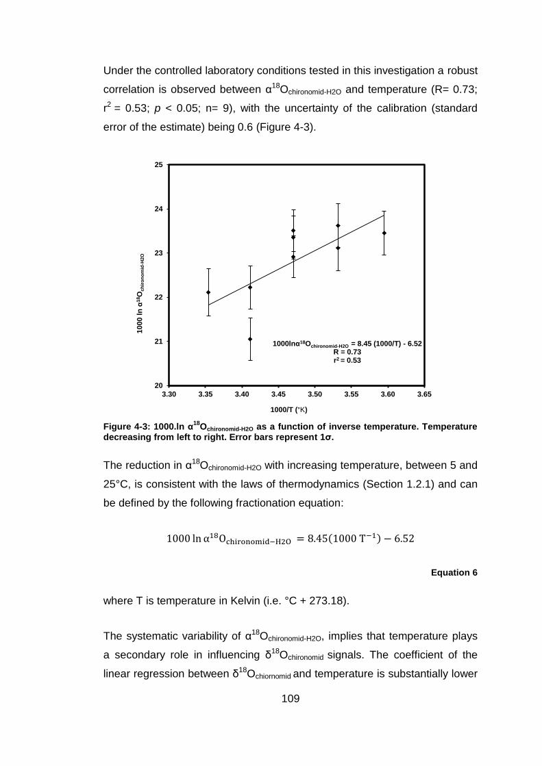
Under the controlled laboratory conditions tested in this investigation a robust
correlation is observed between α18Ochironomid-H2O and temperature (R= 0.73;
r2 = 0.53; p < 0.05; n= 9), with the uncertainty of the calibration (standard
error of the estimate) being 0.6 (Figure 4-3).
Figure 4-3: 1000.ln α18
Ochironomid-H2O as a function of inverse temperature. Temperature decreasing from left to right. Error bars represent 1σ.
The reduction in α18Ochironomid-H2O with increasing temperature, between 5 and
25°C, is consistent with the laws of thermodynamics (Section 1.2.1) and can
be defined by the following fractionation equation:
1000 ln α18Ochironomid−H2O = 8.45(1000 T−1) − 6.52
Equation 6
where T is temperature in Kelvin (i.e. °C + 273.18).
The systematic variability of α18Ochironomid-H2O, implies that temperature plays
a secondary role in influencing δ18Ochironomid signals. The coefficient of the
linear regression between δ18Ochiornomid and temperature is substantially lower
1000lnα18Ochironomid-H2O = 8.45 (1000/T) - 6.52 R = 0.73 r2 = 0.53
20
21
22
23
24
25
3.30 3.35 3.40 3.45 3.50 3.55 3.60 3.65
1000 l
n α
18O
ch
iro
no
mid
-H2O
1000/T (°K)
110
(~ −0.1‰/°C−1) than in mineral precipitates, where oxygen isotope
fractionation has been well defined experimentally and empirically in
carbonates (−0.24‰/°C−1; Kim & O’Neil 1997) and is less well-defined in
biogenic silica (~ −0.2 to −0.5‰/°C−1; Brandriss et al., 1998; Juillet-Leclerc &
Labeyrie 1987; Leng & Barker 2006).
All results plot within 1σ of analytical uncertainty, except for one of the
rearing experiments at 20°C. The reason for the disparity between the two
rearing experiments at this temperature is not known, but could be related to
additional dietary contributions from microorganisms originating from the
decomposition of excess food. The statistical strength of the relationship
between α18Ochironomid-H2O and temperature can be improved by removing this
apparent outlier (R = 0.81; r2 = 0.66; p < 0.05; n= 8). Furthermore, standard
error of the estimate is reduced to 0.4 while the gradient and intercept of the
linear regression is substantially changed so that:
1000 ln α18Ochironomid−H2O = 6.29 (1000 T−1) + 1.16
Equation 7
Given the relatively small size of the data set (n=9), it was decided that the
most pragmatic approach would be to retain this apparent outlier. Replicate
samples for each of the rearing experiments have been prepared, but at the
time of writing had not been analysed due to analytical difficulties at Durham
University. The results from the replicate analyses will help establish whether
the apparent outlier should be retained or excluded from the data set.
The consistency of the findings of this investigation was assessed in relation
to the results obtained by Wang et al. (2009) (Figure 4-4). In their study,
Chironomus dilutus larvae were reared under controlled laboratory conditions
(23°C with a constant diet) in waters with different 18O/16O ratios. The study
reported a strong correlation between δ18Ochironomid (whole larvae) and
δ18OH2O. The results presented in this section bisect the linear regression
observed between δ18Ochirononmid (whole larvae) and δ18OH2O in Wang et al.
111
(2009), with measurements from rearing experiments conducted at
temperatures above/close to 23°C plotting below the line, and measurements
from rearing experiments conducted at temperatures below 23°C plotting
above the line.
Figure 4-4: Open squares represent mean δ18
Ochironomid (whole larvae) vs. δ18
OH2O from Wang et al. (2009). Black diamonds represent average δ
18Ochironomid reared at different
temperatures vs. δ18
OH2O, from this study.
This section documents the first experimental calibration of the relationship
between α18Ochironomid-H2O and temperature (between 5 and 25°C).
Precipitation processes in inorganic systems (e.g. carbonate and silicate) are
known to be associated with temperature-dependant oxygen isotope
fractionations. However, temperature is largely anticipated to have a
negligible influence on oxygen isotope fractionation in organic matter (e.g.
DeNiro & Epstein 1981; Wolfe et al., 2001). The results from this
investigation indicate that temperature may influence α18Ochironomid-H2O in
larvae reared under controlled conditions. However, it should be noted that
the coefficient (~ −0.1‰/°C−1) of the observed relationship is significantly
smaller than the analytical error associated with the measurements. Since
This study δ18Ochironomid = 8.45 x δ18OH2O - 6.52
Wang et al. (2009) δ18Ochironomid = 0.72 x δ18OH2O + 20.24
5
10
15
20
25
30
-20 -15 -10 -5 0 5 10
δ18O
ch
iro
no
mid
(‰
V-S
MO
W)
δ18OH2O (‰ V-SMOW)
112
this data set is relatively small it is recommended that further laboratory- and
field-based calibration studies should be performed to validate these findings.
It is hoped that the results presented in this section will eventually form part
of a larger data set permitting the empirical characterisation of the
relationship between α18Ochironomid-H2O and temperature, which is essential to
the development of this approach as a tool for reconstructing past climates.
The implications of the findings in terms of palaeoclimate reconstructions are
discussed further in Section 4.5.
113
4.3 An investigation of δ18Ochironomid in a near constant natural environment
4.3.1 Site description
Greywell Moor Nature Reserve (latitude 51.25°N longitude – 0.96°W),
situated 70km west-southwest of London in the village of Greywell
(Hampshire, UK), is an area of managed heathland surrounded by arable
farmland (Figure 4-5). After an initial inspection of a series of groundwater
fed ponds within the reserve, a ~10m diameter, shallow (< 1m deep), roughly
circular pond (herein referred to as Greywell Pond) was chosen for
monitoring between May 2011-2013 since it contained the most abundant
chironomid community. The chosen pond has no discernible outflow, draining
through seepage into an adjacent marsh area before ultimately feeding the
River Whitewater (Keatings et al., 2002). A previous monitoring program by
Keatings et al. (2002) indicated that pond water δ18O, temperature and
chemistry remained essentially constant between December 1996 and March
1998 (see Table 4-4). Although laboratory studies are an excellent model for
examining the influence of different parameters on δ18Ochironomid they are
rarely able to fully simulate the complex biological requirements of an
organism, potentially hindering “normal” growth. Greywell pond provides an
ideal “natural culture” for assessing the relationship between δ18Ochironomid and
δ18Olakewater due to the stability of pond water δ18O, temperature and
chemistry at the site.
114
Figure 4-5: Greywell Pond (latitude 51.25°N longitude – 0.96°W). Image modified from Keatings et al. (2002).
Records of average monthly temperature and precipitation between 1981-
2010 were obtained from the Met office database for Odiham meteorological
station (latitude 51.24°N longitude – 0.94°W; 118m above mean sea level),
which is the closest meteorological station to the reserve located 1.8 miles
south-east of Greywell. Mean monthly air temperature varied seasonally, with
maximum values reported in July (21.9°C) and minimum values in February
(1.3°C) (Figure 4-6). Precipitation is generally evenly distributed throughout
the year, with the highest monthly average in October (87.2mm) and lowest
in June (48.5mm) (Figure 4-6).
115
Figure 4-6: Mean minimum and maximum monthly temperature and total monthly precipitation for Odiham (nearest station to Greywell) between 1981 and 2010 (Met Office).
0
5
10
15
20
25
0
10
20
30
40
50
60
70
80
90
100
Jan Feb Mar Apr May Jun Jul Aug Sep Oct Nov Dec
Tem
pe
ratu
re (°
C)
To
tal
Pre
cip
itati
on
(m
m)
Month
Total Precipitation Max Temperature Min Temperature
116
4.3.2 Sampling
Water samples- Water samples were collected at elbow depth from the
centre of the pond (deepest part) in polyethylene bottles at monthly intervals.
On return to the laboratory the water samples were filtered using disposable
cellulose acetate filters (0.2μm pore size) and stored at 4°C, in 5ml screw top
glass vials with no head space, prior to stable isotope analysis at the
University of Liverpool (see Section 4.2.2).
Water Chemistry- Camlab Handylab 1 battery powered hand-held meters
attached to a data logger were used to measure electrical conductivity
(μScm−1), dissolved oxygen concentration (mgL−1) and pH of the pond water.
The meters were calibrated before use in accordance with manufacturer’s
procedures. Repeated measurements (x3) were taken from three roughly
equidistant locations along a transect bisecting the pond, with average
values presented in this thesis.
Water temperature was measured hourly between December 2011 and May
2013, with a Tinytag Aquatic 2 (TG-4100) data logger (accuracy ±0.2°C for
measurements between 0°C and 70°C). The logger was first installed into the
pond in September 2011, however it failed to record any data until December
2011 due to a programming malfunction.
Chironomid Larvae- Chironomid larvae were isolated from surface
sediments washed through a metal sieve (mesh size 1mm) in situ, using fine-
tipped forceps. The larvae were retained in ambient lake water, before being
frozen whole on return to the laboratory. No attempts were made to
differentiate species or instar stage due to low sample abundance, although
the coarse sieve size is likely to have resulted in the preferential retention of
larger 3rd and 4th instars, since the smaller 1st and 2nd instars will have
passed through the mesh.
Following defrosting, head capsules were manually isolated from larval
bodies (Section 4.2.2) before undergoing chemical pretreatment (see Section
3.6 for purification procedure) and δ18O analysis (Section 2.3).
117
4.3.3 Results & discussion
Water chemistry
Mean, minimum and maximum values for water chemistry (May 2011-2013)
and temperature (December 2011-May 2013) are presented in Table 4-4,
alongside data collected by Keatings et al. (2002).
Table 4-4: Mean, minimum and maximum values for monthly water chemistry (May 2011-2013) and average monthly water temperature (December 2011- May 2013) from Greywell Pond. Data presented alongside measurements made by Keatings et al. (2002).
May 2011- 2013
(This study)
March 1997- Feb 1998
(Keatings et al., 2002)
Mean Min Max Mean Min Max
pH 7.0 6.7 7.3 6.87 6.75 6.97
Dissolved
Oxygen (mgL−1)
5.8 3.2 8.0 N/A N/A N/A
Conductivity
(μScm−1)
627 577 660 506 498 514
Temperature (°C) 10.4 10.0 10.6 11.0 10.2 12.3
Pond water chemistry and temperature remained essentially constant over
the duration of the study (Table 4-4 and Figure 4-7). In particular, average
monthly water temperature only exhibited small variations over the
monitoring period, ranging from 10 to 10.6°C. The results from this
investigation are consistent with the findings of Keatings et al. (2002) (Table
4-4), with discrepancies between the studies potentially arising due to
differences in equipment and methodologies adopted.
118
10.0
10.2
10.4
10.6
10.8
Tem
pe
ratu
re (
°C)
570
590
610
630
650
670
Co
nd
uc
tvit
iy (
μS
/cm
-1)
2
3
4
5
6
7
8
9
Dis
so
lved
Oxyg
en
(m
g/L
)
6.5
6.7
6.9
7.1
7.3
7.5
Apr-11 Jul-11 Sep-11 Nov-11 Feb-12 Apr-12 Jul-12 Sep-12 Dec-12 Feb-13 May-13
pH
Date (MM-YY)
Figure 4-7: Evolution of mean monthly pH, conductivity, dissolved oxygen and temperature from Greywell Pond. Each of the variables remain largely stable throughout the sample period supporting the findings of Keatings et al. (2002).
119
δ18Olakewater
Stable isotope analyses were performed on water samples collected from
Greywell Pond at roughly monthly intervals between May 2011 and April
2013, with values ranging between −7.2 to −6.9‰. Average δ18Olakewater
measurements (−7.1‰ ± 0.1) are largely indistinguishable from the values
reported in Keatings et al. (2002). The values are also consistent with non-
evaporated meteoric waters from this part of England (Darling et al., 1996),
with monthly δ18Olakewater plotting on or close to the GMWL (Figure 4-8). The
stability of δ18Olakewater is principally due to the short residence time of water
(~100 minutes) at Greywell Pond (Keatings et al., 2002).
Figure 4-8: Relationship between δ18
O and δD of pond water between May 2011- April 2013. Error bars represent internal precision (±0.1‰) of δ
18Olakewater determinations.
Dashed line represents GMWL and solid line represents the LMWL on to which the data from the site plots.
LMWL δD = 2.69 x δ18O - 26.94
GMWL δD = 8 x δ18O + 10
-48
-47
-46
-45
-44
-43
-7.8 -7.6 -7.4 -7.2 -7.0 -6.8 -6.6 -6.4 -6.2 -6.0
δD
lakew
ate
r (‰
V-S
MO
W)
δ18Olakewater (‰ V-SMOW)
120
Negligible seasonal variations in δ18Olakewater were observed at the site
throughout the sampling period (see Figure 4-9)
Figure 4-9: The evolution of δ18
Olakewater during spring (March, April, May), summer (June, July, August), autumn (September, October, November) and winter (December, January and February) throughout the monitoring period. Error bars represent 1σ of seasonal variability observed δ
18Olakewater measurements.
-7.20
-7.15
-7.10
-7.05
-7.00
-6.95
-6.90
-6.85
Spring Summer Autumn Winter
δ1 8
O l
akew
ate
r (‰
V-S
MO
W)
Season
121
δ18Ochironomid
Oxygen isotope analyses were performed on a total of nine purified
chironomid samples (see Section 3.6 for purification procedure) collected
from Greywell Pond between July 2011 and April 2013. Replicates for each
sample were prepared for analysis, however at the time of writing these had
not been analysed due to laboratory difficulties at Durham University. Since
replicate δ18Ochironomid analyses were not available, an estimate of analytical
uncertainty was based on repeated analyses of IAEA 601 (1σ = ± 0.40‰)
(see Section 2.3.1) as its accepted value is closest to the measured
δ18Ochironomid values.
The oxygen isotope composition of purified chironomid head capsules varied
throughout the duration of the monitoring period, ranging between
+16.1-18.2‰ (α18Ochironomid-lakewater = 1.023-1.025) (Figure 4-10a). The most
striking feature of the seasonal evolution of the δ18Ochironomid signal is the
negative isotope shift of ~ −1.6‰ between spring and summer (Figure
4-10b).
122
-9.0
-8.5
-8.0
-7.5
-7.0
-6.5
-6.0
-5.5
-5.0
16.0
16.5
17.0
17.5
18.0
18.5
19.0
Spring Summer Autumn Winter
δ18O
lakew
ate
r (‰
V-S
MO
W)
δ1
8 O c
hir
on
om
id (‰
V-S
MO
W)
Season
b)
-9.0
-8.5
-8.0
-7.5
-7.0
-6.5
-6.0
-5.5
-5.0
15.0
15.5
16.0
16.5
17.0
17.5
18.0
18.5
19.0
Apr-11 Nov-11 May-12 Dec-12
δ18O
lakew
ate
r (‰
V-S
MO
W)
δ18O
ch
iro
no
mid
(‰
V-S
MO
W)
Month -Year
Chironomid Lake Watera)
Figure 4-10: a) Monthly and b) seasonal evolution of δ18
Ochironomid and δ18
Olakewater over the monitoring period; spring (March, April, May), summer (June, July, August), autumn (September, October, November) and winter (December, January and February). The most striking feature of the seasonal evolution of δ
18Ochironomid signal is the negative isotope
shift (~ −1.6‰) observed between spring and summer.
123
No significant correlation was observed between δ18Ochironomid and
δ18Olakewater, average monthly air temperature, average monthly water
temperature, monthly pH, monthly electrical conductivity or monthly dissolved
oxygen concentration (Table 4-5).
Table 4-5: Correlation between δ18
Ochironomid and monthly δ18
Olakewater, average monthly air temperature, average monthly water temperature, pH, electrical conductivity, and dissolved oxygen concentration.
R r2 p n
δ18Olakewater −0.44 0.20 > 0.05 9
Air Temperature −0.59 0.34 > 0.05 9
Water Temperature −0.72 0.52 > 0.05 6
pH 0.05 0.00 > 0.05 9
Electrical
Conductivity 0.40 0.16 > 0.05 9
Dissolved Oxygen
Concentration 0.15 0.02 > 0.05 9
Wang et al. (2009) demonstrated that ~70% of oxygen atoms in chironomid
biomass (whole larvae) are derived from habitat water under controlled
laboratory conditions. The origin of the remaining ~30% is unclear, but is
likely to be mainly comprised of ingested food (Wang et al., 2009). Similarly,
Nielsen & Bowen (2010) reported that ~10-30% of oxygen in the chitinous
remains of Artemia franciscana is derived directly from diet. Since
δ18Olakewater, temperature and water chemistry at the site remained essentially
constant; the observed variability in δ18Ochironomid may reflect seasonal
changes in the isotopic composition of diet (δ18Odiet). Based on the
proportional contributions (~10-30%), changes in δ18Odiet in the order of
~4-16‰ would have been necessary to facilitate the observed seasonal
124
variability in δ18Ochironomid (Figure 4-10b). The influence of diet on δ18Ochironomid
cannot be quantitatively assessed in this investigation; however a conceptual
framework examining the feasibility of the required magnitude of change in
δ18Odiet will now be constructed.
Chironomid larvae are typically omnivores, deriving nourishment from a
combination of phytoplankton, zooplankton and sedimented detrital material
(including associated microorganisms) (Armitage et al., 1995; Epler 2001;
Oliver 1971; Walker 1987). The relative abundance of these components
varies seasonally in most lakes. Phytoplankton and zooplankton are likely to
make up a significant proportion of larval diets during the spring and summer
months. In contrast, during the autumn and winter, larval diets are anticipated
to be primarily composed of organic detritus and associated microorganisms.
Typically the organic detritus in most lakes is composed of particles that have
formed within the water column (Jones & Grey 2004) and therefore should be
isotopically reflective of lake water. However, at Greywell Pond terrestrial leaf
litter shed by deciduous trees (mainly Corylus) surrounding the pond is likely
to have formed a significant proportion of the available organic detritus.
The isotopic composition of terrestrial plants are typically 18O enriched in
comparison to aquatic plants, as a result of enhanced evapotranspiration
(kinetic isotope fractionation) (Sauer et al., 2001; Sensuła et al., 2006). The
magnitude of the typical offset between terrestrial and aquatic plants
described in Sensuła et al. (2006) is consistent with the δ18Odiet offset
necessary to facilitate the observed variability in δ18Ochironomid at Greywell
Pond (Table 4-6).
125
Table 4-6: Average δ18
O of plants collected within the same ecosystem from Sensuła et al. (2006). Terrestrial plants are on average 4‰ heavier than aquatic plants.
δ18O (‰ V-SMOW)
Terrestrial plants 28.98
Semi-submerged plants 26.81
Submerged plants 24.62
In temperate regions chironomid populations typically pass through two
generations per year (bivoltine), with the main emergences occurring in the
spring and late summer/early autumn (Tokeshi 1995). The development rate
of Chironomus riparius larvae under controlled laboratory conditions at 10°C,
the average monthly water temperature at Greywell Pond, was ~4 months
(see Table 4-2). If a similar development time is assumed for the chironomid
larvae at Greywell Pond, adults emerging in the late summer/ early autumn
are likely to have completed the majority of their life cycle during the spring/
early summer. In contrast, adults emerging in the spring will have completed
the majority of their life cycle during the previous autumn, overwintering as
3rd/4th instars.
Growth and development can be temporarily arrested or slowed during
unfavourable conditions, in a process known as diapause. This survival
strategy is commonly adopted in poikilotherms (an organisms who’s internal
body temperature varies) such as Chironomidae (Armitage et al., 1995;
Brooks et al., 1997; Hahn & Denlinger 2011). The initiation and termination of
diapause can be triggered by changes in a number of different environmental
stimuli (e.g. temperature, photoperiod, dissolved oxygen concentration, food
abundance and/or quality) (Armitage et al., 1995). Diapause offers a survival
advantage, permitting the synchronisation of life cycles with periods suitable
for growth, development and reproduction (Hahn & Denlinger 2011). Insects
generally adopt two main strategies in mitigating the energetic costs
associated with diapause: a) they accumulate micronutrient reserves (e.g.
126
carbohydrate, protein and lipid) prior to the onset of diapause and b) they
limit metabolic activity during diapause (Nation 2008; Pinder 1986). Feeding,
and even restricted growth, may still occur during diapause in some insects
along with the synthesis of amino acids required to support anabolic
activities, catabolic respiratory metabolism and postdiapause development
(Godlewski et al., 2001; Hahn & Derlinger 2011; Sonoda et al., 2007).
Following the termination of diapause, larval development re-commences
with the metabolism of the remaining polysaccharide reserves, e.g. trehalose
and glycogen, accumulated prior to and during diapause.
Given the envisaged seasonal change in δ18Odiet at Greywell Pond,
polysaccharides synthesised during the autumn and winter will differ
isotopically from those synthesised during the spring or summer. This may
potentially explain the observed variability in δ18Ochironomid signals. The
increase in average seasonal δ18Ochironomid from summer to winter (Figure
4-10b) may indicate a gradual proportional change in the relative contribution
of terrestrial and aquatic components in the chironomid larvae diet. The
hypothesis outlined above could not be experimentally verified in this
investigation. The implications of the findings in terms of palaeoclimate
reconstructions are discussed in greater detail in Section 4.5.
An alternative argument is that the observed variability in δ18Ochironomid may be
related to vital effects. Seasonal variability in δ13C and δ15N signals from
chironomid larvae has been attributed to vital effects in previous studies (e.g.
Grey et al., 2004). However, since chironomid species were not identified in
this investigation, this hypothesis could not be explored.
127
4.4 An investigation of δ18Ochironomid in a series of lakes from the Attenborough Nature Reserve
4.4.1 Site description
The Attenborough Nature Reserve (~170ha) (latitude 52.53°N longitude -
1.24°W) is located within the catchment of the River Trent, 7km southwest of
the city of Nottingham (East Midlands, UK) (Figure 4-11). The reserve, a
designated Site of Special Scientific Interest (SSSI), contains a series of
semi-connected, shallow (maximum depth 5.2m) former gravel pits that have
been allowed to fill naturally following the termination of gravel extraction
(Sayer & Roberts 2001). Drier areas of scrub and grassland as well as native
woodland separate the lakes. Four of the lakes within the reserve were
chosen for monthly monitoring between June 2011 and May 2013: Main
Pond (extracted 1939-1960), Church Pond (extracted 1962-1965), Clifton
Pond (extracted 1964-1968) and Beeston Pond (extracted 1941-1951). A
summary of the basic physical characteristics of each lake is provided in
Table 4-7.
Table 4-7: Summary of physical lake characteristics (modified from Jones et al., in prep).
Pond Area (ha) Max Depth (m) Inflow Outflow
Main 24 5.0 Yes Yes
Beeston 0.9 2.7 Yes Yes
Church 9.6 5.2 No No
Clifton 18.6 3.3 No No
128
Derbyshire
Leicestershire
Nottingha
mshire
Attenborough
Nature Reserve
Figure 4-11: Attenborough Nature Reserve (latitude 52.53°N longitude −1.24°W), Nottingham, UK. The reserve is close to the confluence of the River Trent and River Erewash. Marked on the map (black triangle) are the approximate sampling locations in each of the monitored lakes (map modified from Cross 2009).
129
Main and Beeston ponds are both hydrologically open systems, with surface
inflows and outflows. Main Pond can essentially be considered as a wide
section of river, with water from the River Erewash flowing through it before
entering the River Trent (Jones et al., in prep). In contrast Church and Clifton
ponds are both isolated from the main lake chain, as well as one another,
with no surface inflows or outflows. The lakes provide a perfect opportunity to
assess the relationship between δ18Ochironomid and δ18Olakewater in hydrologically
different natural settings subjected to essentially the same climatic,
geographical and geological conditions.
Meteorological data for the monitoring period was obtained from an
automated weather station at the University of Nottingham’s Sutton
Bonnington Campus (pers. comm. Matt Jones), which is approximately ~11
miles south of the nature reserve. Mean monthly air temperatures varied
seasonally, with maximum (16.8°C) and minimum (2.3°C) mean values
recorded in the summer and early spring respectively.
Monthly total rainfall ranged from 8 to 112mm over the sampling period. The
seasonal distribution of precipitation was fairly even, with the highest total
amount of precipitation observed during summer months (356mm), while the
lowest amount of precipitation was recorded during spring (291mm). Both
total monthly precipitation and mean monthly temperature compared well
with average meteorological data from the East Midlands (1981-2010)
(Figure 4-12).
130
-5
0
5
10
15
20
25
0
20
40
60
80
100
120
Jun-11 Sep-11 Dec-11 Mar-12 Jun-12 Sep-12 Dec-12 Mar-13
Tem
pe
ratu
re (°
C)
To
tal
Pre
cip
itati
on
(m
m)
Date (mm-yy)
0
5
10
15
20
25
0
10
20
30
40
50
60
70
80
90
Jan Feb Mar Apr May Jun Jul Aug Sep Oct Nov Dec
Tem
pe
ratu
re (°
C)
To
tal
Pre
cip
itati
on
(m
m)
Month
Total Precipitation Max Temperature
Min Temperature
Figure 4-12: a) Minimum and maximum monthly temperature and average monthly precipitation for the East Midlands between 1981 and 2010 (Met Office data). b) Minimum and maximum monthly temperature and total monthly precipitation between July 2011 to May 2013 from University of Nottingham Sutton Bonnington Campus, which is approximately ~11 miles south of the nature reserve (pers. comm. Matt Jones).
a)
b)
131
4.4.2 Sampling
Sampling at the Attenborough Nature Reserve was undertaken in
collaboration with Dr. Suzanne McGowan (University of Nottingham).
Samples were collected from a fixed point marked by an anchored buoy
(Figure 4-11), which was roughly located in the deepest part of each lake.
Water samples- see Section 4.3.2.
Water Chemistry- A YSI 600QS-O-M multi-probe attached to a 650MDS
data logger was used to measure vertical profiles for conductivity (mScc−1),
temperature (°C), dissolved oxygen concentration (mgL−1) and pH of the
water column at 50cm intervals. Average values for each of the measured
variables are presented in this thesis. The meter was calibrated before use in
accordance with manufacturer’s procedures
Chironomid Larvae- Sediment samples (two buckets full) were collected
using an Ekman grab from each pond. On return to the laboratory the
sediments were washed through a 1mm mesh and live chironomid larvae
were isolated using fine tipped forceps. The larvae were frozen whole. No
attempts were made to differentiate species or instar stage due to low
sample abundance, although the coarse sieve size is likely to have resulted
in the preferential retention of larger 3rd and 4th instars, since the smaller 1st
and 2nd instars will have passed through the mesh.
Following defrosting, head capsules were manually isolated from larval
bodies (Section 4.2.2) before undergoing chemical pretreatment (Section
3.6) and δ18O analysis (Section 2.3).
132
4.4.3 Results & Discussion
Water temperature
Minimum, maximum and mean monthly lake water temperatures from each
lake throughout the sampling period (May 2011- June 2013) are presented in
Table 4-8.
Table 4-8: Mean, minimum and maximum water temperature from each lake during the monitoring period.
Water Temperature (°C)
Pond Mean Minimum Maximum
Main 10.7 ± 5.9 3.5 20.5
Beeston 11.0 ± 6.0 3.2 20.5
Church 10.5 ± 6.1 2.7 21.8
Clifton 10.7 ± 6.2 3.0 21.0
The main features of water temperature are virtually identical in each of the
studied lakes, with maximum temperatures recorded during the summer
months and minimum values recorded in the winter (Figure 4-13).
133
Figure 4-13: Monthly average lake water temperature from each of the monitored ponds over the sampling period.
During the monitoring period water temperature was largely homogenous
throughout the water column (Figure 4-14). Some thermal stratification was
apparent in all of the lakes during the summer/autumn months probably as a
result of the difference in temperature between the colder ground water
inflow and the warmer water column.
!
y = 0.56x + 19.91
r2 = 0.42
R = 0.65
10
12
14
16
18
20
22
24
26
-10 -8 -6 -4 -2 0
δ1
8O
ch
iro
no
mid
(‰
V-S
MO
W)
δ18Olake water (‰ V-SMOW)
Main Pond Church Pond Clifton Pond Beeston Pond
134
Figure 4-14: Average seasonal temperature profiles for each lake. A degree of thermal stratification can be observed during the summer and autumn months probably related to poor mixing and the cooling influence of ground waters.
!
0.0
0.5
1.0
1.5
2.0
2.5
3.0
3.5
10.5 11.0 11.5 12.0 12.5 13.0 13.5
Wa
ter
De
pth
(m
)
Water Temperature (°C)
Beeston Pond Church Pond Clifton Pond Main Pond
WINTER SPRING
SUMMER AUTUMN
135
Water chemistry
Mean monthly conductivity, dissolved oxygen concentration and pH from
each lake throughout the sampling period (May 2011- June 2013) are
presented in Table 4-9. The measured parameters in each of the lakes are
largely comparable with each other and all showed seasonal variations. The
causes for the variations in conductivity, dissolved oxygen concentration and
pH are beyond the scope of this study but are likely to be related to changes
in local hydrological and/or biological conditions.
Table 4-9: Mean conductivity, dissolved oxygen concentration and pH of lake water at each site from June 2011-May 2013.
Pond Conductivity
(mScc−1)
Dissolved
Oxygen (mgL−1)
pH
Main 0.9 ± 0.2 13.1 ± 4.0 8.2 ± 0.6
Beeston 0.6 ± 0.1 12.1 ± 2.0 8.2 ± 0.5
Church 0.5 ± 0.1 12.6 ± 2.1 8.4 ± 0.7
Clifton 0.6 ± 0.0 12.2 ± 2.1 8.4 ± 0.3
Conductivity- Mean monthly conductivity ranged between 0.5 and
1.1 mScc−1 across the four lakes during the monitoring period, with the
highest value recorded in Main Pond in March 2012 and lowest value
recorded in Church Pond in November 2012.
Dissolved oxygen concentration- Mean monthly dissolved oxygen
concentration ranged between 5.4 and 19.8 mgL−1 across the four lakes
during the monitoring period, with the highest value recorded in Main Pond in
March 2012 and the lowest value recorded in Church Pond in September
2011.
136
pH- Mean monthly pH ranged between 7.7 and 10.0 across the four lakes
during the monitoring period, with the highest values recorded in Main Pond
in July 2011 and lowest values recorded in Main Pond in September 2011.
A summary of mean lake water conductivity, dissolved oxygen concentration
and pH from each of the lakes over the duration of the monitoring period is
presented in Figure 4-15.
0.2
0.4
0.6
0.8
1.0
1.2
1.4
Co
nd
uctv
itiy
(m
Scc
-1)
0
5
10
15
20
25
Dis
so
lved
Oxyg
en
(m
gL
-1)
7
8
9
10
11
Apr-11 Jul-11 Nov-11 Feb-12 May-12 Aug-12 Dec-12 Mar-13 Jun-13
pH
Month-Year
Figure 4-15: Mean monthly lake water conductivity, dissolved oxygen concentration and pH from each of the sampled lakes throughout the duration of the study period.
!
y = 0.56x + 19.91
r2 = 0.42
R = 0.65
10
12
14
16
18
20
22
24
26
-10 -8 -6 -4 -2 0
δ1
8O
ch
iro
no
mid
(‰
V-S
MO
W)
δ18Olake water (‰ V-SMOW)
Main Pond Church Pond Clifton Pond Beeston Pond
137
δ18Olakewater
Stable isotope analyses were performed on surface water samples from
each of the lakes on monthly intervals throughout the monitoring period
(Table 4-10). Lake water samples collected over the study period yielded
δ18O values ranging from −6.4‰ to +0.1‰, with mean δ18Olakewater
measurements being ~ 4‰ higher in the hydrologically closed lakes (Church
and Clifton) than in the open lakes (Main and Beeson) (Table 4-10).
Table 4-10: Summary of mean δ18
Olakewater from each of the sampled sites between June 2011 and May 2013.
δ18Olakewater (‰ V-SMOW)
Pond Mean Minimum Maximum
Main −6.8 ± 1.3 − 9.0 −4.7
Beeston −6.2 ± 1.5 − 8.9 −4.0
Church −2.5 ± 2.2 − 6.4 −0.1
Clifton −2.4 ± 2.3 −6.7 +0.1
Surface water samples from Main and Beeston ponds plot on, or close to the
GMWL, with values becoming more enriched in 18O during periods of greater
evaporative enrichment (i.e. during the summer) (Figure 4-16). In contrast,
δ18Olakewater from Church and Clifton ponds generally plot on a LEL,
suggesting evaporation had a stronger influence in these lakes probably due
to the longer residence times.
138
Figure 4-16: Relationship between δ18
Olakewater and δDlakewater from each lake throughout the duration of the sampling period. The dashed line represents the GMWL, while the solid line represents the LEL determined from linear regression of all surface water data. The majority of the samples plot below the GMWL, indicating a degree of evaporative enrichment of the heavy isotopes in each lake.
No correlation was observed between monthly δ18Olakewater and average
monthly δ18Oprecipitation over the sampling period from Keyworth
(Nottinghamshire, UK), the closest available record to the Attenborough
Nature Reserve (record provided by British Geological Society pers. comm.
Melanie Leng) (R= 0.14; r2 = 0.02; p > 0.05; n = 33) prior to the flood event at
the site. The offsets between δ18Olakewater and δ18Oprecipitation are likely to have
arisen as a consequence of local hydrological conditions at each of the lakes.
The seasonal evolution of δ18Olakewater (Figure 4-17b) is most likely to reflect
the preferential partitioning of water molecules containing light isotopes of
hydrogen and oxygen into the vapour phase during evaporation, with the
highest values observed in each lake during the summer/early autumn. The
influence of the evaporative enrichment is greatest in the closed lakes, with
monthly δ18Olakewater measurements ~ 2.6‰ higher in the summer compared
to the winter months; whereas average enrichment of only ~ 1.4‰ is
observed between winter and summer δ18Olakewater measurements in the open
lakes (Main and Beeston).
LEL δD = 5.65 x δ18O - 9.49
r² = 0.99
GMWL δD = 8 x δ18O + 10
-70
-60
-50
-40
-30
-20
-10
0
-10 -8 -6 -4 -2 0
δD
lakew
ate
r (‰
V-S
MO
W)
δ18Olakewater (‰ V-SMOW)
Main Pond Church Pond Clifton Pond Beeston Pond
139
Figure 4-17: a) Evolution of δ18
Olakewater from each lake throughout the duration of the monitoring. b) Average seasonal evolution of δ
18Olakewater from each lake throughout
the duration of the monitoring; spring (March, April, May), summer (June, July, August), autumn (September, October, November) and winter (December, January and February).
-10
-9
-8
-7
-6
-5
-4
-3
-2
-1
0
1
Feb-11 Jun-11 Sep-11 Dec-11 Apr-12 Jul-12 Oct-12 Jan-13 May-13 Aug-13
δ18O
lakew
ate
r (‰
V-S
MO
W)
Date (mm-yy)
!
-9
-7
-5
-3
-1
Spring Summer Autumn Winter
δ18O
%lake%water%(‰
%V0SMOW)%!
Season
Main Beeston Church Clifton
-9
-7
-5
-3
-1
Spring Summer Autumn Winter
δ18O
lakew
ate
r (‰
V-S
MO
W)
Season
a)
b)
140
During periods of high water levels, Church and Clifton ponds are liable to
become connected to the main lake chain through a series of overflow pipes
and weirs. The substantial negative shift in δ18Olakewater values observed in all
of the sites in the winter of 2012 was associated with a flood event. This flood
event was caused by a combination of prolonged intensive precipitation (see
Figure 4-12a) and poor maintenance of the system of weirs throughout the
lake chain (i.e. weirs became blocked with debris). Interestingly, the isotopic
composition of the lake water in the closed lakes (Church and Clifton) failed
to fully recover to pre-flood values before the end of the monitoring period, 7
months after the initial flood.
141
δ18Ochironomid
Oxygen isotope analyses were performed on purified chironomid head
capsules (see Section 3.6 for purification procedure) isolated from larvae on
near bi-monthly intervals from each of the studied lakes. Replicates for each
sample were prepared for analysis, however at the time of writing these had
not been analysed due to laboratory difficulties at Durham University. Since
replicate δ18Ochironomid analyses were not available, an estimate of analytical
uncertainty was based on repeated analyses of IAEA 601 (1σ = ± 0.40‰)
(see Section 2.3.1) as its accepted value is closest to the measured
δ18Ochironomid values.
Spatial and temporal variations were observed in δ18Ochironomid measurements
throughout the duration of the monitoring period, with values ranging
between 13.1 and 20.8‰ (α18Ochironomid-H2O = 1.018-1.027) (Table 4-11). The
~ 4‰ disparity between δ18Ochironomid from hydrologically open (Main and
Beeston) and closed (Church and Clifton) lakes (Table 4-11) is consistent
with the offsets observed between δ18Olakewater (Table 4-10).
Table 4-11: Summary of mean, minimum and maximum δ18
Ochironomid observed at each pond between July 2011- May 2013.
δ18Ochironomid (‰ V-SMOW)
Pond Hydrological
Status
Mean Minimum Maximum
Main Open
+14.9 ± 0.9 +13.6 +16.5
Beeston +15.0 ± 1.0 +13.1 +16.2
Church Closed
+19.0 ±1.1 +16.9 +20.4
Clifton +19.3 ±1.3 +17.2 +20.8
The evolution of δ18Ochironomid and δ18Olakewater throughout the monitoring
period is presented in Figure 4-18.
142
Figure 4-18: Evolution of δ18
Ochironomid (solid line) and δ18
Olakewater (dashed line) in each of the lakes between June 2011- May 2013. Note the dramatic decrease in δ
18Olakewater
in the hydrologically closed (Church and Clifton) ponds after November 2012 is associated with flooding at the reserve.
143
A moderate linear relationship was observed between δ18Ochironomid and
δ18Olakewater across the lakes monitored in this study (R= 0.65; r2 = 0.42; p <
0.05; n = 53) (Figure 4-19).
Figure 4-19: Relationship between the measured δ18
Ochironomid and measured δ
18Olakewater from July 2011- May 2013. Dashed line represents linear regression
between δ18
Ochironomid and δ18
Olakewater.
The significance of the correlation between δ18Ochironomid and δ18Olakewater can
be improved by removing data following the flood event (R= 0.85; r2 = 0.73; p
< 0.05; n = 33) (Figure 4-20). The reassessment of the data excluding
measurements after November 2012 reduces the uncertainty of the
calibration between δ18Ochironomid and δ18Olakewater from ±1.8 to ±1.2.
δ18Ochironomid = 0.56 x δ18Olake water + 19.91 R = 0.65 r2 = 0.42
10
12
14
16
18
20
22
24
-10 -8 -6 -4 -2 0
δ18O
ch
iro
no
mid
(‰
V-S
MO
W)
δ18Olakewater (‰ V-SMOW)
Main Pond Church Pond Clifton Pond Beeston Pond
144
Figure 4-20: δ18
Ochironomid vs. δ18
Olakewater from July 2011- November 2012. Samples plotting on the lower left side of the figure are from hydrologically open (Main and Beeston), while data plotting on the upper right side are from hydrologically closed (Church and Clifton) lakes.
The coefficient of determination between δ18Ochironomid and δ18Olakewater in the
reanalysed data (Figure 4-20) is still <1 (r2 = 0.73), implying that other factors
may have influenced δ18Ochironomid. The cause(s) of the lower than anticipated
coefficient of determination must invoke either variable α18Ochironomid-H2O or
partial equilibration of oxygen atoms incorporated within chironomid head
capsules with a source other than lake water. Some of the potential causes
of the lower than anticipated coefficient of determination will now be briefly
discussed.
δ18Ochironomid = 0.76 x δ18Olake water + 20.06 R = 0.85 r² = 0.73
10
12
14
16
18
20
22
24
-10 -8 -6 -4 -2 0
δ18O
ch
iro
no
mid
(‰
V-S
MO
W)
δ18Olakewater (‰ V-SMOW)
Main Pond Church Pond Clifton Pond Beeston Pond
145
Temperature-dependant α18Ochironomid-H2O
The results presented in Section 4.2 (see Figure 4-3) indicate that
α18Ochironomid-H2O varies systematically with temperature. A linear relationship
is also apparent in the samples collected from Attenborough prior to the
November 2012 flooding (R = 0.55; r2 = 0.31; p < 0.05; n = 33) (Figure 4-21).
Figure 4-21: 1000lnα18
Ochironomid-H2O as a function of inverse average monthly water temperature in Kelvin. Temperature decreases from left to right.
The temperature dependence of α18Ochironomid-H2O between ~3 and 22°C
(temperature range observed in the sampled lakes) can be expressed by the
following equation:
1000ln α18Ochironomid-H2O = 10.52 (1000T−1) – 16.21
Equation 8
The coefficient of the relationship between δ18Ochironomid and temperature is
largely indistinguishable in the laboratory (Section 4.2) and field-based
studies (~ −0.1‰/°C−1 in both studies). Unsurprisingly the uncertainty of the
1000lnα18Ochironomid-H2O = 10.52 x (1000/T) - 16.21 R = 0.55 r² = 0.31
16
17
18
19
20
21
22
23
24
25
3.35 3.40 3.45 3.50 3.55 3.60 3.65
1000. L
n(α
ch
iro
no
mid
-H2O)
1000/T (K)
Main Pond Beeston Pond Church Pond Clifton Pond
146
calibration is considerably smaller in the controlled laboratory study (±0.63) in
comparison to the field data (±1.14). This is most likely to be a reflection of
the influence of environmental variability in the field-based calibration
studies. It should be noted that offsets are also observed between laboratory
and experimentally derived fractionation equations in the carbonate system
(Lécuyer et al., 2013).
Diet
Based on the results presented in Section 4.3 it may be speculated that the
metabolism of oxygen atoms directly from dietary sources may have
contributed to the lower than anticipated correlation coefficient between
δ18Ochironomid and δ18Olakewater. However, this could not be assessed in this
investigation.
Water chemistry
No correlation was observed between δ18Ochironomid and any of the measured
in-lake parameters (e.g. dissolved oxygen concentration, pH and electrical
conductivity) (Table 4-12).
Table 4-12: Correlation between δ18
Ochironomid and, monthly pH, monthly electrical conductivity, and monthly dissolved oxygen concentration.
Main and Beeston (Open) Church and Clifton (Closed)
R r2
n p-value R r2 n p-value
pH −0.38 0.15 16 >0.05 −0.39 0.15 17 >0.05
Electrical
Conductivity −0.04 0.00 16 >0.05 0.07 0.00 17 >0.05
Dissolved
Oxygen −0.52 0.27 16 >0.05 0.22 0.05 17 >0.05
147
δ18Olakewater seasonality
Seasonal changes in chironomid metabolism coupled with seasonality in
δ18Olakewater, δ18Odiet and in-lake variables (e.g. photoperiod, water
temperature, pH, productivity) provide strong evidence to suggest that
δ18Ochironomid may reflect seasonal signals. However, the results from this
study indicate that although mean δ18Ochironomid values varied seasonally in
each lake, with minimum values generally observed in the late summer,
these differences were not statistically significant (one-way ANOVA,
p > 0.05).
148
-9
-8
-7
-6
-5
-4
13
14
15
16
δ18O
lakew
ate
r (‰
V-S
MO
W)
δ18O
ch
iro
no
mid
(‰ V
-SM
OW
)
Main Beeston
-5
-4
-3
-2
-1
0
17
18
19
20
21
Spring Summer Autumn Winter
δ18O
lakew
ate
r(‰
V-S
MO
W)
δ18O
ch
iro
no
mid
(‰ V
-SM
OW
)
Season
Church Clifton
a)
b)
Figure 4-22: a) Mean seasonal changes in δ18
Ochironomid (solid line) and δ18
Olakewater (dashed line) observed in the hydrologically open and, b) closed ponds. No statistical significant seasonal differences were observed between δ
18Ochironomid (one-way
ANOVA, p > 0.05). Observed variability in δ18
Ochironomid signatures is largely in anti-phase with changes in δ
18Olakewater.
149
Integration of environmental isotopic signature
High-resolution contemporary calibration studies of this nature generally
assume that the isotopic composition of a measured compound is reflective
of conditions at the time of sampling. In reality isotopic turnover in biologically
inert structures, such as chironomid head capsules, is likely to lack sufficient
temporal resolution to respond instantaneously to changing environmental
conditions. Larval development can only proceed following periodic ecdysis,
with the formation of a new cuticle involving the partial re-digestion of the old
cuticle, as well as the assimilation of new material (van Hardenbroek et al.,
2010; Iovino 1975; Nation 2008). In other insects excessive cuticular
sclerotisation in the latter instar stages restricts digestion to structural weak
points, facilitating moulting (Nation 2008). Therefore, it can be reasonably
assumed that restricted head capsule digestion will occur during 3rd/4th instar
stages. Since the biosynthesis of chironomid head capsules is not uniform
over the year (Heiri et al., 2012), one may anticipate that δ18Ochironmid
represents an integrated signal throughout larval development, weighted
towards periods of more intense growth (i.e. spring/summer), rather than a
discrete set of environmental conditions.
The reassessment of the relationship between δ18Ochironomid and δ18Olakewater
integrated over varying months suggests that isotopic turnover in chironomid
head capsules is ~ 5 months (Table 4-13), which is consistent with
development rates reported in Section 4.2.3. Delayed isotopic turnover may
have contributed to the lower than expected correlation coefficient observed
in this investigation and potentially explain the relatively muted response in
δ18Ochironomid to the flood event (Figure 4-18).
150
Table 4-13: Statistical correlation between δ18
Ochironomid and δ18
Olakewater with different lake water integration periods, along with associated standard error of the estimate. It should be noted that data after November 2012 were excluded from the data set. The strongest statistical relationship is observed when a 5-month integration is applied.
Number of Months
Integrated
R r2 p n Standard error
of the estimate
1 0.85 0.73 < 0.05 33 1.21
2 0.87 0.75 < 0.05 32 1.14
3 0.89 0.79 < 0.05 30 1.05
4 0.90 0.81 < 0.05 30 0.99
5 0.91 0.82 < 0.05 30 0.97
6 0.90 0.82 < 0.05 27 0.97
It appears likely that δ18Ochironomid signatures reflect an integrated
environmental signal over the duration of the chironomid life cycle. Further
extensive field-based calibration studies assessing seasonal variability in
δ18Ochironomid in a wide range of lakes are necessary to validate this
hypothesis.
The implications of the findings in terms of palaeoclimate reconstructions are
discussed in greater detail in Section 4.5.
151
4.5 Implications of contemporary calibration studies for palaeoclimate reconstructions
The results presented in this chapter lend support to the hypothesis that
contemporary δ18Ochirononmid signals are strongly reflective of habitat water in
which the larvae grew. The compilation of complementary calibration data
sets demonstrates the existence of a strong linear correlation between
δ18Ochironomid and δ18Olakewater (R= 0.95; r2 = 0.90; p < 0.05; n = 58) (Figure
4-23).
Figure 4-23: Plot of δ18
Ochironomid and δ18
Olakewater constructed using data prior to the flood event (data after November 2012 excluded) from Attenborough and published field (Verbruggen et al., 2011) and laboratory (Wang et al., 2009) calibration data sets.
δ18Ochironomid = 0.70 x δ18Olake water + 20.11
R = 0.95 r² = 0.90
5
10
15
20
25
30
-20 -15 -10 -5 0 5 10
δ18O
ch
iro
no
mid
(‰
V-S
MO
W)
δ18Olakewater (‰ V-SMOW)
Verbruggen et al (2011) Wang et al (2009) AttenboroughVerbruggen et al. (2011) Wang et al. (2009)
152
The strength of the linear relationship implies that stratigraphic changes in
δ18Ochironomid can be used to directly infer past δ18Olakewater, using the following
equation:
δ18Olakewater =(δ18Ochironomid − 20.11)
0.70
Equation 9
It should be noted however that no chemical pre-treatments were applied in
the studies conducted by Wang et al. (2009) or Verburggen et al. (2011), with
analyses performed on whole chironomid larvae and head capsules isolated
from surface sediments respectively. Given the influence of the chemical pre-
treatments employed in this investigation (see Chapter 3), direct comparison
of the different data sets is potentially problematic.
The predictive power of this model was evaluated by using Equation 9 to
estimate average δ18Olakewater prior to the November 2012 flood event from
each of the monitored lakes using average δ18Ochironomid as an input (Table
4-14).
Table 4-14: Assessment of model performance [δ18
Olakewater = (δ18
Ochironomid -20.11)/ 0.70] for reconstructing average δ
18Olakewater values at Attenborough lakes prior to the
November 2012 flood, using average δ18
Ochironomid as an input.
Pond Average
δ18Ochironomid
Average
δ18Olakewater
Modelled
δ18Olakewater
Δ18Oactual-
model
Main +15.1 −6.2 −7.2 +0.98
Beeston +15.3 −5.5 −6.8 +1.32
Church +19.1 −1.4 −1.5 +0.11
Clifton +19.3 −1.1 −1.2 +0.04
153
Although the performance of the model is encouraging, with an average
Δ18Oactual-model of ~ +0.6‰, it is clear from the results presented in Chapter 4
that the interpretation of δ18Ochironomid signals is not as straightforward as
originally anticipated.
In contrast to inorganic compounds, temperature-dependant fractionations
are expected to be largely absent/negligible during the formation of
chironomid head capsules (e.g. Verbruggen et al., 2010b; 2011; Wang et al.,
2009; Wooller et al., 2004; 2008). The results from laboratory (Section 4.2)
and field (Section 4.4) based calibration studies are the first clear
demonstrations that δ18Ochironomid signals are not immune to the complexities
surrounding temperature-dependant α18Ochironomid-H2O. Both laboratory and
field-based studies observed a systematic linear relationship between
α18Ochironomid-H2O and temperature; however the linear regressions of the two
studies differed greatly from one another (unpaired t-test; p < 0.05). The
discrepancies between the two studies may be related to the influence of
interlinked environmental processes operating in the field-based study.
Considering the discrepancies in the relationship between α18Ochironomid-H2O
and temperature observed in the calibration studies the two data sets were
combined to produce a chironomid-water oxygen isotope fractionation
equation (Figure 4-24):
1000ln α18Ochironomid-H2O = 6.30 (1000T−1) – 0.85
Equation 10
Equation 10 can be used to quantify α18Ochironomid-H2O as a function of
temperature and will be utilised in the following chapter. It should be
considered that the coefficient of the relationship between δ18Ochironomid and
temperature (~ −0.1‰/°C−1) observed in the calibration studies presented in
this chapter is considerably smaller than the reported analytical uncertainties
(Section 2.3). However, the results clearly indicate a statistically significant
relationship between α18Ochironomid-H2O and temperature.
154
Figure 4-24: Plot of 1000lnα18
O chironomid-H2O as a function of inverse temperature. It should be noted that data after November 2012 has been excluded from the Attenborough data set.
The metabolism of oxygen atoms with different dietary isotopic signatures
during chitin biosynthesis may also potentially complicate the interpretation of
δ18Ochironomid signals (Section 4.3). However, in most cases it may be argued
that δ18Olakewater and δ18Odiet will be strongly correlated since the majority of
the dietary components will have formed within the water column
(Verbruggen et al., 2011). Future studies should focus on the analyses of
larval gut content to establish the influence of δ18Odiet on the δ18Ochironomid
signal. It also appears likely that δ18Ochironomid of an assemblage will reflect an
integrated environmental isotopic signature weighted towards periods of
most intensive growth.
The results presented in this chapter provide the foundation for translating
stratigraphic changes in δ18Ochirononmid into estimates of past δ18Olakewater,
which will be explored in Chapter 5. However, inherent uncertainties
surrounding the confounding influences on δ18Ochironomid signals restrict the
predictive power of Equation 9; therefore chironomid-inferred δ18Olakewater can
only really be considered as a first order estimate.
1000lnα18Ochironomid-H2O = 6.30 (1000/T) - 0.85 R² = 0.09
15
16
17
18
19
20
21
22
23
24
25
3.30 3.35 3.40 3.45 3.50 3.55 3.60 3.65
1000ln
α18
Och
iro
no
mid
-H2O
1000/T (°K)
Main Pond Church Pond Clifton Pond
Beeston Pond Cultures
155
Chapter 5 Lake water palaeothermometry; combined δ18O analyses of authigenic carbonate and chironomid remains from a Late-glacial sediment core, Hawes Water (UK).
5.1 Introduction
The development of quantitative palaeotemperature proxies is essential for
improving our understanding of the likely impacts of future climate change.
This chapter focuses on the evaluation of a novel approach for reconstructing
palaeotemperatures, by measuring δ18O of co-occurring chironomid head
capsules and bulk carbonate from a Late-glacial sediment sequence
retrieved from Hawes Water (UK). The climate of the Late-glacial period is of
considerable interest to climate modellers, since it represents one of the
most recent periods of natural, high amplitude, climate change; characterised
by prolonged cold periods (stadials) interspersed by warmer episodes
(interstadials) (Lang et al., 2010). However, terrestrial based palaeoclimate
reconstructions from this period are scarce in the UK and are mostly transfer
function based (e.g. Atkinson et al., 1987; Bedford et al., 2004; Brooks et al.,
2012; Brooks & Birks 2000; Brooks & Langdon 2014). Hawes Water has
been the focus of several comprehensive multi-proxy studies, which have
demonstrated that the sediment sequence at the site contains a remarkably
coherent record of climate change (for review see Bedford et al., 2004, Jones
et al., 2002, Marshall et al., 2002). Moreover, sediments from the site have
been shown to contain abundant chironomid remains (e.g. Bedford et al.,
2004) making Hawes Water an ideal testing ground for the development of
the chironomid-carbonate palaeothermometer.
156
5.1.1 Chapter aims and objectives
This chapter aims to contribute to the development of the chironomid-
carbonate palaeothermometer. This will be achieved by: -
Producing a high-resolution δ18Ochironomid record from Hawes Water.
Comparing stratigraphic changes in δ18Ochironomid with an existing high-
resolution δ18Obulk_carbonate (Thomas, unpublished) record from the
same sediment core.
Estimating past lake water temperature from stratigraphic changes in
δ18Ochironomid and δ18Obulk_carbonate.
157
5.2 Hawes Water: background and context
5.2.1 Setting
Hawes Water is a small (8ha, max depth ~ 12m, ~ 10m above sea level),
oligotrophic, hard-water lake ~ 40km north of Lancaster (northwest England)
(54°10’58”N, 2°48’10”W; Figure 5-1) (Bedford et al., 2004; Jones et al.,
2011). The lake, along with its smaller sister basin (Little Hawes Water), is
situated within a shallow depression in a Carboniferous limestone catchment
characterised by low limestone hills (Jones et al., 2002).
Figure 5-1: A map showing the location of Hawes Water (Jones et al., 2002).
The lake is predominantly groundwater fed but it also receives inputs from
precipitation and from its sister basin, via a small stream (Jones et al., 2002).
Seepage and stream-flow onto the adjacent Hawes Water Moss are the
primary outflows of the lake (Bedford et al., 2004; Jones et al., 2002; 2011;
Lang et al., 2010 Marshall et al., 2002). The contemporary δ18Olakewater
(−6.4‰ to −5.5‰) at the site broadly reflects local precipitation, owing to
short residence times and a positive precipitation:evaporation balance
(Marshall et al., 2002). Furthermore, the site is subject to minimal seasonal
evaporative enrichment (~ 0.7‰) between surface and bottom waters during
summer months (Marshall et al., 2002).
158
The contemporary lake is surrounded by a terrestrialised marl bench
containing sediments up to 12m thick; with each meter corresponding to
roughly 1000 years worth of accumulation based on published sedimentation
rates (Marshall et al., 2002). The presence of this terrestrialised marl bench
demonstrates that lake levels were once higher than they are today. The
sediment sequence at Hawes Water is uninterrupted from the start of the
Late-glacial period through to the Holocene (Bedford et al., 2004; Jones et
al., 2002; Lang et al., 2010; Oldfield 1960). The composite stratigraphy of the
sediments from Hawes Water were first described by Oldfield (1960) and are
characterised by a clay section overlain by micrites (limestone formed of
calcareous particles), deposited during the Late-glacial interstadial, followed
by another clay unit corresponding to the deposition during the Younger
Dryas (Marshall et al., 2002). This composite stratigraphy conforms well to
the classic tripartite stratigraphic model of Late-glacial sites across North-
west Europe (e.g. Lowe & Walker 1997). A detailed interpretation of pollen,
chironomid and lithological data have been provided in Jones et al. (2002),
while Marshall et al. (2002) discussed the stable isotope records from Hawes
Water (Figure 5-2).
159
Figure 5-2: Summary diagram of multi-proxy data, including stable isotopic composition of carbonates, lithology, pollen groups and inferred catchment vegetation, and warm and cold chironomid abundances from Hawes Water for the Late-glacial and early Holocene. Stable isotope analyses were conducted on homogenised micrite samples. Abbreviations: AP, arboreal pollen; NAP, non-arboreal pollen; LOI, loss of ignition- used to determine organic matter content (%) of sediment samples through the comparison of sample weights before and after ignition (105°C for 24 hours). Diagram from Marshall et al. (2002).
Chironomid
160
5.3 Materials and methods
5.3.1 Sediment core
Colleagues from the University of Exeter collected three parallel sediment
cores from the northern margin of the lake (054°11.032’ N, 002°48.119’W,
elevation 7m), using a large-diameter Russian corer. The cores were sub-
divided into 1cm segments and freeze dried. A limited amount of sediment
(10-20g) from selected intervals, spanning the glacial-interstadial transition
(HW1), Late-glacial interstadial (HW2) and the Younger Dryas stadial (HW3),
were made available for analyses in this investigation. A reliable
chronological framework for the site has proved elusive to date (Jones et al.,
2002). Efforts have been hampered by a dearth of suitable materials and the
plateau effect associated with 14C AMS dating (Ammann & Lotter 1989; Lowe
1991). In the absence of a reliable chronology, the results of this
investigation will be presented within the zonal stratigraphic framework,
outlined in Marshall et al. (2002) (see Figure 5-2), based on the correlation of
δ18Obulk_carbonate records from the two cores.
The freeze-dried sediment samples (10-20g) were washed through 210 and
90μm mesh sieves with deionised water. The retained residue was briefly
(~10 seconds) sonicated, to reduce particles adhering to the surface of the
head capsules, before being re-sieved. Aliquots of the sieve residue were
transferred into a grooved perspex-sorting tray (Bogorov sorter with grooves
5mm deep, 5mm wide), and chironomid larval head capsules were picked
under a binocular microscope (x25). No attempts were made to identify the
chironomid species represented in each sub-sample, due to limited sediment
availability. Isolated head capsules were stored at 4°C in glass vials
containing MilliQ water. The isolated heads were re-examined, providing an
opportunity to remove any obvious contamination or miss-identified material,
prior to chemical pre-treatment with 2:1 DCM: MeOH. 0.25M HCl, 0.25M
NaOH for 24 hours at 20°C (see Section 3.6) and stable isotope analysis
(see Section 2.2).
161
5.4 Results and interpretation
5.4.1 Stratigraphic changes in δ18Ochironomid
Oxygen isotope analyses were performed on purified (treated with 2:1 DCM:
MeOH, 0.25M HCl, 0.25M NaOH solutions for 24 hours at 20°C) chironomid
head capsules isolated from selected sediment horizons. The stratigraphic
resolution of the record varied due to sample availability; however where
possible analyses were performed every 2cm. No δ18Ochironomid analyses
could be performed between 312-320cm due to low head capsule
abundance and poor yield following chemical pre-treatment. All samples
were measured in replicates (x3) and converted onto the V-SMOW scale.
The reproducibility of replicate δ18Ochironomid measurements was
±0.7‰ (1σ). δ18Ochironomid values ranged between +11.6-16.7‰ (mean =
+14.1‰; n = 42), with the highest values recorded during Late-glacial
interstadial (HW2) and the lowest during the Younger Dryas (HW3) (see
Table 5-1 and Figure 5-3). The poor reproducibility of replicate δ18Ochironomid
measurements is most likely to be reflective of inter-individual variations,
since each analysis was performed on ~ 5-20 individual head capsules
equating to a weight of 60 ±10µg. However, it should also be reiterated that
the analytical precision based on repeated analyses of IAEA 600, 601 and
602 references materials was between ±0.4-0.6‰ (1σ).
162
Table 5-1: Summary of average δ18
Ochironomid in each of the identified sub-divisions.
Depth (cm)
δ18Ochironomid (‰ V-SMOW)
Min Max Average
e
Glacial-interstadial
transition (HW1)
357-368
+12.7
+15.8
+13.8
Late-glacial
interstadial (HW2)
306-356
+13.6
+16.7
+15.1
Younger Dryas (HW3)
268-305
+11.6
+14.6
+12.8
The δ18Ochironomid record is presented alongside a high-resolution (1cm)
δ18Obulk_carbonate record (analytical precision = > 0.1‰) (Thomas, unpublished)
produced from the same sediment sequence, in Figure 5-3. The δ18O records
from the independent archives are strikingly similar to one another (R = 0.84,
r2 = 0.70, P < 0.05, n = 44), but the δ18Ochironomid record is on average ~ 19‰
higher compared to the δ18Obulk_carbonate record. The δ18O records indicate
climate instability, with lower values associated with demonstrably colder
climatic conditions.
163
260
270
280
290
300
310
320
330
340
350
360
370
10 11 12 13 14 15 16 17 18
Dep
th (
cm
)
δ18Ochironomid (‰ V-SMOW)
-7 -6 -5 -4 -3
δ18Obulk_carbonate (‰ V-PDB)
Event A
Event B
Event C
Event D
Glacial-interstadial transition (HW1)
Younger Dryas (HW3)
Late-glacial interstadial (HW2)
!
260
270
280
290
300
310
320
330
340
350
360
370
10 11 12 13 14 15 16 17 18
De
pth
(c
m)
δ18Ochironomid (‰ V-SMOW)
1σ = 0.68
for chironomids
Figure 5-3: Hawes Water δ18
Ochironomid (black circle) and δ18
Obulk_carbonate (grey crosses; Thomas, unpublished) records. The amplitude of the two records differ with δ
18Ochironomid varying by 5.1‰, while the δ
18Obulk_carbonate record varies by 2.7‰
throughout the measured length of the core. Both δ18
O records are characterised by a series of negative isotope excursions (labelled Event A-D) prior to the onset of the Younger Dryas (HW3). Replicate measurements from individual samples were used to estimate uncertainty in the δ
18Ochironomid record (1σ = ±0.68‰). Note that the two records
are presented on separate scales due different reference standards used during the analyses of the two materials.
164
The δ18Ochironomid and δ18Obulk_carbonate records are both characterised by a
series of negative isotope excursions (labelled Event A-D in Figure 5-3) prior
to the onset of the Younger Dryas (HW3). The negative isotope excursions
reflect significant, short-lived deteriorations in climatic conditions and are
correlated with changes in other independent climate proxy records reported
across the UK (e.g. Brooks & Birks 2000; Mayle et al., 1997; Walker et al.,
1993; Walker 1982), Europe (e.g. Eicher & Sigenthaler 1976; von
Grafenstein et al., 1999; Lotter et al., 1992) and in ice core records from
Greenland (e.g. Johnsen et al., 1992). The characteristics of these negative
isotope excursions are summarised in Table 5-2.
Table 5-2: δ18
O characteristics of major negative isotope excursions. * denotes poor sampling resolution restricting the interpretation of the signal.
δ18Ochironomid (V-SMOW) δ18Obulk_carbonate (V-PBD)
Event λ (cm) -ve +ve Shift λ (cm) -ve +ve Shift
A 362-366 1.2 1.1 −0.1 361-367 0.4 1.1 +0.7
B 344-354 1.0 1.5 +0.5 342-353 1.8 1.9 +0.1
C 332-338 1.8 2.6 +0.8 332-338 0.8 1.1 +0.3
D* 320-326 2.1 0.8 −1.3 314-330 1.0 0.7 −0.3
165
The evolution of δ18Ochironomid throughout the Late-glacial period will now be
discussed in greater detail within the zonal stratigraphic framework outlined
in Marshall et al. (2002).
357-368 cm: Glacial-interstadial transition (HW1)- In this section
δ18Ochironomid values ranged between +12.7 and +15.8‰, fluctuating
around a mean of +13.8‰. Increases in δ18Ochironomid are coherent with
climate amelioration as indicated by increases in the abundance of
thermophilic chironomid taxa (e.g. Chironomus, Dicrotendipes,
Psectrocladius) (Bedford et al., 2004) and non-arboreal pollen (Jones
et al., 2002) (see Figure 5-2).
306-356cm: Late-glacial interstadial (HW2)- Broadly speaking the
δ18Ochironomid signature displays a bipartite structure, with values
gradually increasing from the base of the zone to a peak of +16.7‰ at
332cm, before steadily declining prior to the onset of the Younger
Dryas (HW3). Increases in δ18Ochironomid are again coherent with
changes in chironomid taxa (Bedford et al., 2004) and plant
communities (Jones et al., 2002) (see Figure 5-2).
The δ18Ochironomid signal is punctuated by three negative isotope
excursions (Event B-D). The first of the oscillations (Event B) is
associated with a ~ 1.0‰ decline in δ18Ochironomid values, whereas the
oscillations in the latter part of the zone are associated with a decline
of ~ 1.8‰ (Event C) and ~ 2.1‰ (Event D).
268-305cm: Younger Dryas stadial (HW3)- Mean δ18Ochironomid
values for this period are on average ~ 2.5‰ lower than during the
Late-glacial interstadial, with values ranging between +11.6 and
+14.6‰. The onset of the zone is marked by a rapid decline in
δ18Ochironomid, after which values increase slightly before stabilising at
~ +12.5‰ and rising again prior to the onset of the Holocene.
166
Decreases in δ18Ochironomid are associated with a rise in cold water
adapted chironomid species (e.g. Sergentia, Paracladius and
Heterotrissocladius) (Bedford et al., 2004) and the expansion of
grassland and herb communities (Jones et al., 2002) (see Figure 5-2).
The variability observed in the independent δ18O archives is largely coherent,
although small discrepancies in the magnitude and timing occur in some
parts of the core. For example, the response in the δ18Ochironomid following
‘Event A’ lags a few centimetres behind the δ18Obulk_carbonate record; whereas
the onset of Younger Dryas (HW3) occurs first in the δ18Ochironomid record. The
general coherence of the δ18O records indicates a strong similarity in the
mechanisms involved in the incorporation of δ18O signals in both archives. In
contrast to Verbruggen et al. (2011) (Section 1.4.3) the amplitude of
variability observed in this study is greatest in the δ18Ochironomid record, which
is reflected in the gradient of the relationship between the independent δ18O
archives [δ18Ochironomid = 1.5 x δ18Obulk_carbonate + 21.7]. An exception to this
general trend is ‘Event B’, which is less pronounced in the δ18Ochironomid
record. This discrepancy is likely to be an artefact of sample resolution, with
other stratigraphic records failing to report ‘Event B’ due to poor sampling
resolution.
167
5.4.2 Quantitative palaeoclimate reconstructions from stratigraphic changes in δ18Obulk_carbonate and δ18Ochironomid
In his seminal work, Urey (1947) observed that the fractionation of oxygen
isotopes between calcite of marine organisms and ocean water (α18Ocalcite-
H2O) was sensitive to temperature. In cases of equilibrium, the measured
fractionation between the two phases can be used to estimate temperature at
the time of calcification based on the thermodynamics of the mineral that is
being precipitated (Epstein et al., 1953; McCrea 1950; Urey 1947). Increases
in temperature are associated with a decrease in the fractionation between
the water and the measured compound. In contrast to chironomids, α18Ocalcite-
H2O has been well constrained experimentally and empirically (e.g. McCrea
1950; Epstein et al., 1953; Kim & O’Neil 1997). Based on these findings
Craig (1965) developed the first palaeotemperature equation [T (°C) = 16.0 –
4.14 (δ18Ocarbaonte - δ18Owater) + 0.13 (δ18Ocarbonate - δ
18Owater)2]. Today, one of
the most commonly used palaeotemperature equations is that of Kim and
O’Neil (1997), which was re-expressed in a more convenient form by Leng
and Marshall (2004):
𝐓 = 𝟏𝟑. 𝟖 − 𝟒. 𝟓𝟖(𝛅𝟏𝟖𝐎𝐜𝐚𝐫𝐛𝐨𝐧𝐚𝐭𝐞 − 𝛅𝟏𝟖𝐎𝐇𝟐𝐎)𝟐 + 𝟎. 𝟎𝟖(𝛅𝟏𝟖𝐎𝐜𝐚𝐫𝐛𝐨𝐧𝐚𝐭𝐞 − 𝛅𝟏𝟖𝐎𝐇𝟐𝐎)
Equation 11
where: T refers to water temperature (°C), δ18Ocalcite is the oxygen isotope
composition of the CO2 produced by the reaction between the sample calcite
with phosphoric acid compared to the V-PDB standard, δ18Owater is the
oxygen isotope composition of the water from which the calcite is precipitated
from compared to the V-SMOW standard. It should be noted that
temperature estimates made using Equation 11 are lower than those
calculated using the traditional Craig (1965) palaeotemperature equation or
its derivatives (Leng & Marshall 2004).
This approach was first quantitatively applied to estimate past ocean
temperatures from foraminifera in deep-sea cores (Emiliani 1954, 1966), and
has since been applied in numerous terrestrial and marine-based
investigations. However, a fundamental problem of oxygen isotope
168
palaeothermometry in lacustrine settings is that both δ18Ocarbonate and
δ18Olakewater are required in order to resolve a value for temperature (Hodell
et al., 2012). In most lacustrine-based studies a value for δ18Olakewater is often
assumed from contemporary calibration studies. However, the assumption
that hydrological conditions have remained constant over the time period
studied in this investigation is unlikely to be valid (Marshall et al., 2002).
Based on the results presented in Chapter 4 stratigraphic changes in
δ18Ochironomid can be used to directly infer past δ18Olakewater, using Equation 9
(see Section 4.5):
𝛅𝟏𝟖𝐎𝐥𝐚𝐤𝐞𝐰𝐚𝐭𝐞𝐫 =(𝛅𝟏𝟖𝐎𝐜𝐡𝐢𝐫𝐨𝐧𝐨𝐦𝐢𝐝 − 𝟐𝟎. 𝟏𝟏)
𝟎. 𝟕𝟎
Equation 9
Chironomid-inferred δ18Olakewater estimates for Hawes Water using this
approach range between −12.1‰ and −4.9‰ (Table 5.3), bracketing
contemporary δ18Olakewater values (−6.4‰ to −5.5‰).
169
Table 5-3: Summary of chironomid-inferred δ18
Olakewater estimates using the experimental calibration relationship between δ
18Ochironomid and δ
18Olakewater [δ
18Olakewater
= (δ18
Ochironomid-20.11)/0.70].
Reconstructed δ18Olakewater (V-SMOW)
Depth (cm) Min Max Average
Glacial-interstadial
transition (HW1)
357-368 −10.5 −6.1 −8.4
Late-glacial
interstadial (HW2)
306-356 −9.3 −4.9 −7.2
Younger Dryas (HW3) 268-305 −12.1 −7.9 −10.5
Assuming equilibrium carbonate precipitation, chironomid-inferred
δ18Olakewater estimates were used in conjunction with co-existing
δ18Obulk_carbonate measurements to estimate calcification temperatures using a
palaeotemperature equation ( Equation 11), with the resulting values ranging
between −9°C and +11°C (~ ±7°C error based on the reproducibility of
δ18Ochironomid measurements (±0.68‰)) (Figure 5-4). The uncertainty of the
temperature estimates (±7°C) is disconcerting, particularly when considering
that chironomid-inferred mean July air temperatures were shown to vary by
~6°C throughout the whole Late-glacial period from the same site (Bedford et
al., 2004).
170
260
270
280
290
300
310
320
330
340
350
360
370
-15 -10 -5 0 5 10 15 20
Dep
th (
cm
)
Temperature (°C)
Event A
Event C
Event D
Younger Dryas (HW3)
Late-glacial interstadial (HW2)
Glacial-interstadial transition (HW1)
Event B
Figure 5-4: Reconstructed summer lake water temperatures (solid line) calculated using the calcite-water equilibrium equation [T°C = 13.8 − 4.58 (δ
18Ocarbonate -δ
18Olakewater)
+ 0.08 (δ18
Ocarbonate -δ18
Olakewater)] (Leng & Marshall 2004) and chironomid-inferred δ
18Olakewater. Temperature estimates are associated with errors of ~ ±7°C (dashed line)
based on the reproducibility of δ18
Ochironomid measurements (±0.68‰).
171
Correction for potential isotope exchange induced by the chemical pre-
treatments adopted in this investigation (2:1 DCM: MeOH, 0.25M HCl, 0.25M
NaOH for 24 hours at 20°C) fails to completely eliminate the unrealistic
temperature estimates below zero, although values are moved in a positive
direction (Table 5-4).
Table 5-4: Summary of summer lake water temperature and δ18
Olakewater from derived from the conjunctive use of δ
18Obulk_carbonate and δ
18Ochirononmid after +0.88‰ correction
has been applied to account for potential isotope exchanges induced during chemical pre-treatment.
δ18Olakewater (‰ V-SMOW) Temperature (°C)
Min Max Average Min Max Average
Glacial-interstadial
transition (HW1)
−9.3 −4.9 −7.5 −1.9 +11.9 +3.4
Late-glacial
interstadial (HW2)
−8.1 −3.6 −5.9 +2.6 15.8 8.3
Younger Dryas
(HW3)
−10.9 −6.7 −9.2 −4.6 +8.3 +0.2
Although absolute temperature estimates using this approach are largely
unrealistic the relative temperature changes obtained are comparable with
other studies. For example, the average temperature drop between the Late-
glacial interstadial (HW2) and the Younger Drays (HW3) reported in this
investigation is ~8°C; in comparison Marshall et al. (2002) reported a ~7-8°C
drop in average summer temperatures during the same period based on the
δ18Obulk_carbonate, whereas Bedford et al. (2004) reported a ~6°C drop during
the same period based on C-IT estimates from Hawes Water.
172
5.5 Potential causes for unrealistic temperature estimate
The chironomid-carbonate palaeothermometer tested in this investigation
relies on several fundamental assumptions: i) δ18Ochironomid is a reliable
δ18Olakewater proxy, ii) the independent δ18O archives must have formed
simultaneously from waters with a common δ18Olakewater and temperature, iii)
both archives should be free from contamination and, iv) not be subjected to
any post-depositional alterations. The largely unrealistic temperature
estimates obtained using this approach implies that one, or more, of these
assumptions have been violated in some respect. Each of the assumptions
will now be looked at in more detail.
The results presented in Chapter 4 demonstrate that although a strong linear
correlation does exist between δ18Ochironomid and δ18Olakewater, confounding
factors can complicate the interpretation of δ18Ochironomid signals. The inherent
uncertainties surrounding the calibration of the relationship between
δ18Ochironomid and δ18Olakewater are likely to have a deleterious influence on
chironomid-inferred δ18Olakewater estimates, and therefore ultimately
temperature reconstructions. Laboratory- (Section 4.2) and field- (Section
4.4) based studies identified that temperature has a confounding influence on
δ18Ochironomid signals. Although this relationship is poorly characterised the
results presented in Chapter 4 were used to define a chironomid-water
oxygen isotope fractionation equation, which can be used to quantify
α18Ochironomid-H2O as a function of temperature (see Section 4.5):
1000ln α18Ochironomid-H2O = 6.30 (1000T−1) – 0.85
Equation 10
The chironomid-water oxygen isotope fractionation equation (Equation 10)
can be used in conjunction with the carbonate-water oxygen isotope
fractionation equation [1000lnα18Ocalcite-H2O = 18.03 (1000 T−1) – 32.42] (Kim
& O’Neil 1997) to simultaneously infer changes in temperature and
δ18Olakewater from paired δ18Ochironomid and δ18Obulk_carbonate measurements, using
the following methodology:
173
For carbonate
𝟏𝟎𝟎𝟎𝐥𝐧𝛂𝟏𝟖𝐎𝐜𝐚𝐫𝐛−𝐇𝟐𝐎 = 𝒂𝒄𝒂𝒓𝒃 + 𝒃𝒄𝒂𝒓𝒃 ∙ 𝟏
𝑻
Equation 12
For chironomids
𝟏𝟎𝟎𝟎𝐥𝐧𝛂𝟏𝟖𝐎𝐜𝐡𝐢𝐫𝐨𝐧−𝐇𝟐𝐎 = 𝒂𝒄𝒉𝒊𝒓𝒐𝒏 + 𝒃𝒄𝒉𝒊𝒓𝒐𝒏 ∙ 𝟏
𝑻
Equation 13
Note that:
𝛂𝟏𝟖𝐎𝐜𝐚𝐫𝐛−𝐇𝟐𝐎 =𝟏𝟎𝟎𝟎 + 𝛅𝟏𝟖𝐎𝐜𝐚𝐫𝐛
𝟏𝟎𝟎𝟎 + 𝛅𝟏𝟖𝐎𝐇𝟐𝐎 𝐚𝐧𝐝 𝛂𝟏𝟖𝐎𝐜𝐡𝐢𝐫𝐨𝐧−𝐇𝟐𝐎 =
𝟏𝟎𝟎𝟎 + 𝛅𝟏𝟖𝐎𝐜𝐡𝐢𝐫𝐨𝐧
𝟏𝟎𝟎𝟎 + 𝛅𝟏𝟖𝐎𝐇𝟐𝐎
Therefore
𝛂𝟏𝟖𝐎𝐜𝐚𝐫𝐛−𝐜𝐡𝐢𝐫𝐨𝐧 =𝟏𝟎𝟎𝟎 + 𝛅𝟏𝟖𝐎𝐜𝐚𝐫𝐛
𝟏𝟎𝟎𝟎 + 𝛅𝟏𝟖𝐎𝐜𝐡𝐢𝐫𝐨𝐧 =
𝛂𝟏𝟖𝐎𝐜𝐚𝐫𝐛−𝐇𝟐𝐎
𝛂𝟏𝟖𝐎𝐜𝐡𝐢𝐫𝐨𝐧−𝐇𝟐𝐎
Equation 14
and
𝐥𝐧𝛂𝟏𝟖𝐎𝐜𝐚𝐫𝐛−𝐜𝐡𝐢𝐫𝐨𝐧 = 𝐥𝐧𝛂𝟏𝟖𝐎𝐜𝐚𝐫𝐛−𝐇𝟐𝟎−𝐥𝐧𝛂𝟏𝟖𝐎𝐜𝐡𝐢𝐫𝐨𝐧−𝐇𝟐𝟎
Equation 15
Substituting Equation 12 and Equation 13 into Equation 14 and Equation 15
174
𝟏𝟎𝟎𝟎 𝐥𝐧 {𝟏𝟎𝟎𝟎 + 𝛅𝟏𝟖𝐎𝐜𝐚𝐫𝐛
𝟏𝟎𝟎𝟎 + 𝛅𝟏𝟖𝐎𝐜𝐡𝐢𝐫𝐨𝐧} = (𝐚𝐜𝐚𝐫𝐛 − 𝐚𝐜𝐡𝐢𝐫𝐨𝐧) + (𝐛𝐜𝐚𝐫𝐛 − 𝐛𝐜𝐡𝐢𝐫𝐨𝐧) ∙
𝟏
𝐓
Equation 16
δ18Ochirononmid and δ18Obulk_carbonate are the measured values for each sample,
acarb and bcarb are constant values published in Kim and O’Neil (1997), while
achiron and bchiron are derived from Equation 10. Substitution of the appropriate
values into Equation 16 allows the calculation of 1/T in K, which can then be
used in either Equation 12 or Equation 13 to calculate a value for
α18Ochiron-H2O or α18Ocarb-H2O, and thus permit the calculation of δ18Olakewater.
However, even when accounting for the influence of temperature, the
chironomid-carbonate palaeothermometer still produces results that are
largely below zero (~ −10°C and ~ +11°C) (Table 5-5). This implies that; i)
the characterisation of the relationship between α18Ochironomid-H2O and
temperature is not valid in this circumstance, ii) one or more of the
fundamental assumptions (see above) have been violated during the
adoption of this approach or iii) variables that influence α18Ochironomid-H2O have
been overlooked. For example inaccurate determination of growth water
temperature and/or δ18O of environmental water can lead to imprecise
fractionation equations.
175
Table 5-5: Summary of summer lake water temperature and δ18
Olakewater derived from the conjunctive use of δ
18Obulk_carbonate and δ
18Ochirononmid measurements.
δ18Olakewater (‰ V-SMOW) Temperature (°C)
Min Max Average Min Max Average
Glacial-interstadial
transition (HW1)
−10.2 −5.9 −18.4 −7.6 +6.9 −1.4
Late-glacial
interstadial (HW2)
−8.9 −4.7 −7.0 −3.7 +11.1 +2.8
Younger Dryas
(HW3)
−11.5 −7.4 −9.9 −9.6 +4.4 −4.7
Disparities in the temporal resolution of the two independent δ18O archives
may have contributed to the deleterious palaeotemperature reconstructions
obtained using this approach. For example, the analysed 1cm bulk carbonate
segments may represent several years worth of accumulation whereas the
chironomid head capsules isolated from the same layer may only represent a
few months/years worth of accumulation. Furthermore, disparities in the
timing of calcification and chironomid development could potentially account
for the unrealistic temperature estimates obtained using the chironomid-
carbonate palaeothermometer. An existing contemporary monitoring program
reported that authigenic carbonates are precipitated close to conventional
carbonate isotopic equilibrium at Hawes Water, in response to increased
photosynthetic activity during the summer months (June – August) (Marshall
et al., 2002). Subsequently δ18Obulk_carbonate is likely to reflect summer lake
water conditions. In contrast, δ18Ochironomid is likely to reflect an integrated
environmental signal throughout the life of the larvae, weighted towards
periods of more intense growth (Section 4.4.3). However, the strong
correlation between the two records (Figure 5-3) implies that the independent
archives are likely to have recorded the same environmental signal, although
176
the higher variability observed in the δ18Ochironomid record may reflect the
incorporation of different seasonal signals within the δ18Ochironomid signature
and/or differences in the temporal resolution of the two archives. This
discrepancy may also reflect genuine differences in the sensitivity of the
independent δ18O archives. Such an observation should be treated with a
degree of caution since comparisons are being drawn from records with
different sampling resolutions and analytical precisions. In order to fully
evaluate potential differences in the sensitivity of the two proxies, the
resolution of the δ18Ochironomid record needs to be improved, particularly during
periods of demonstrably colder conditions. However, such periods are
associated with low head capsule abundances and therefore would require
extensive sediment processing to obtain sufficient samples (> 50μg) for δ18O
analyses.
Due to insufficient quantities of individual carbonate micro and macrofossils
colleagues from the University of Exeter performed δ18O analyses on bulk
sediments, which are likely to have contained both authigenic and biogenic
carbonates (including marl, molluscs, ostracods as well as detrital
carbonates). If possible δ18O analyses should not be performed on bulk
sediments since individual carbonate components are associated with unique
mineral-water isotope fractionation effects (von Grafenstein et al., 1999; Leng
& Marshall 2004). Marshall et al. (2002) have indicated that the Late-glacial
carbonate sequence at Hawes Waters is likely to be predominantly
composed of authigenic carbonates. However, varying contributions from
different carbonate components throughout the length of the Hawes Water
core may have contributed to the unrealistic palaeotemperature
reconstructions obtained in this investigation.
177
It is assumed that the sequential treatment of chironomid samples with DCM:
MeOH (2:1), HCl (0.25M), NaOH (0.25M) for 24 hours at 20°C, yielded
samples of a sufficient purity so that contamination did not have a detrimental
influence on δ18O analysis. The effectiveness of the chemical pre-treatments
could not be confirmed since no assessment of the level of contamination
was made prior to or after chemical pre-treatment. However, the chemical
pre-treatments adopted in this investigation were associated with average
∆18Ountreated-treated of −3.3‰ (n= 28; 1σ = 1.4) (Table 5-6), with the statistical
correlation between δ18Obulk_carbonate and δ18Ochironomid increasing slightly
following chemical pre-treatment (Figure 5-5).
178
Table 5-6: Comparison of δ18
Ochironomid from chironomid samples that have and have not been subjected to chemical pre-treatment.
δ18Ochironomid (‰ V-SMOW)
Depth (cm) Treated Untreated Δ18OUntreated-treated
268 13.9 19.7 5.8
270 12.9 18.8 5.9
286 12.5 14.3 1.7
296 11.6 13.3 1.7
297 12.4 14.9 2.5
298 11.9 14.9 3.0
300 12.7 17.1 4.4
302 14.6 18.5 3.9
304 14.3 20.7 6.4
306 14.3 16.8 2.5
308 15.2 17.6 2.4
310 14.6 17.5 2.9
312 14.6 18.7 4.1
326 15.6 19.3 3.7
330 15.4 18.3 2.9
332 16.7 19.4 2.7
334 14.5 19.3 4.8
336 14.1 18.0 3.9
338 15.9 19.8 3.9
342 15.8 19.2 3.4
348 14.8 17.3 2.8
354 15.5 18.3 2.9
356 14.4 18.4 4.0
358 15.8 20.1 4.3
360 13.6 16.8 3.2
362 13.8 14.3 0.5
364 12.7 15.2 2.5
366 13.9 14.7 0.8
Average 3.3
1σ 1.4
179
Figure 5-5: Correlation between a) untreated (square) and b) treated (diamond) δ
18Ochironomid vs. δ
18Obulk_carbonate. The correlation between the archives improves after
chemical pre-treatment.
The chemical composition of chitin is thought to remain largely unchanged
for tens of thousands of years under favourable depositional environments
(e.g. high sedimentation rates and anoxia) (Stankiewicz et al., 1997a;
1997b). Verbruggen et al. (2010a) reported the presence of chitin-derived
moieties in Late-glacial chironomid remains. In contrast, preliminarily
chromatographic screening of chironomid remains in this investigation, using
pyrolysis gas chromatography mass spectrometry (Py-GC-MS) techniques,
suggests that chitin-derived complexes were largely absent in the limited
180
number of samples tested (pers. comm. Reichart, Utrecht University). The
chironomid remains analysed were largely composed of protein-derived
compounds along with a series of alkene/alkanes. The macromolecular
structure of the tested chironomid remains from Hawes Water are
characteristic of the formation of aliphatic (geo)polymers during diagenesis,
via the polymerisation of liberated lipid molecules (Baas et al., 1995; Briggs
1999; Cody et al., 2011; Gupta et al., 2009; Stankiewicz et al., 2000). The
alphatic component of fossil arthropods is bound to the degraded chitin-
protein residue through ester linkage to form the geopolymer (Cody et al.,
2011). The conditions governing the kinetics of this transformation are largely
unknown, therefore the influence of the formation of geopolymers on the
δ18Ochironomid signature at Hawes Water is difficult to ascertain. However,
clearly diagenetic alterations have the potential to reset, or at least alter, the
original δ18Ochironomid signature. Additionally, chitin-protein complexes within
chitinous biomass are known to undergo various condensation reactions post
mortem, resulting in the formation of numerous compounds that may or may
not be indigenous to the original insect remains (Tripp et al., 2004). Based on
the observation made in this investigation it is recommended that the integrity
of the chironomid remains should be assessed through chromatographic
separation prior to δ18O analyses.
Since the formation of geopolymers involves the diagenesis of oxygen-
bearing compounds present in the original material, a large proportion of
oxygen atoms may be derived from the original head capsules. Given the
similarity between the δ18Ochironomid and the δ18Obulk_carbonate records, one may
argue that any diagenetic alterations that took place at Hawes Water must
have produced a systematic offset (i.e. shifted δ18Ochironomid by more or less a
fixed value). For example, an average shift of ~ +2.5‰ is necessary to
largely eliminate unrealistic temperature estimates below 0°C. However, it
should be noted that this offset produces some unrealistically high
temperature estimates indicating that the diagenetic processes may not have
been systematic (Table 5-7).
181
Table 5-7: Summary of δ18
Olakewater and temperature estimates derived using chironomid-carbonate palaeothermometer with a +2.5‰ offset applied for diagenetic alteration.
δ18Olakewater (‰ V-SMOW) Temperature (°C)
Zone Min Max Average Min Max Average
Glacial-interstadial
transition (HW1)
−7.0 −2.6 −5.2 +6.8 +20.6 +12.6
Late-glacial
interstadial (HW2)
−5.8 −1.3 −3.6 +11.4 +24.5 +17.0
Younger Dryas
(HW3)
−8.5 −4.4 −6.9 +4.2 +17.1 +8.9
Ultimately the true cause(s) of the unrealistic temperature estimates returned
by the chironomid-carbonate palaeothermometer is difficult to establish.
However, the available preliminary results tentatively indicate that both
confounding influences on δ18Ochironomid and diagenetic alteration of the
chironomid remains are the principal mechanisms responsible for the
unrealistic temperature reconstructions obtained using the chironomid-
carbonate approach.
182
Chapter 6 Conclusion
The remains of chironomid larvae are often one of the most abundant
biogenic components preserved in lacustrine sediments and have recently
received increasing attention as a tool for inferring past δ18Olakewater, and
indirectly past climate. The main aims of this research (as described in
Section 1.5) were focused on the development of δ18Ochironomid as a tool for
inferring past climates. The early chapters of this thesis concentrated on the
development of analytical and preparatory procedures in the analyses of
δ18Ochironomid, whereas the latter chapters focused on the interpretation of
δ18Ochironomid signals in contemporary and stratigraphic settings.
The absence of a standardised procedure for the preparation of chironomid
remains for δ18O analysis has prevented inter-laboratory comparisons,
hampering the development of the δ18Ochironomid approach. Non-amino
polysaccharide impurities (both compositional and exogenous) present within
chitinous biomass have a deleterious influence on δ18O determinations.
Therefore, in order to produce meaningful δ18Ochironomid measurements efforts
should be made to limit impurities. Based on the results of a systematic
investigation presented in Chapter 3, it is recommend that chironomid
samples are sequentially soaked in DCM: MeOH (2:1), HCl (0.25M), NaOH
(0.25M) solutions for 24 hours at 20°C, prior to δ18O analysis. It is hoped that
this procedure can form the basis for the standardisation of preparatory
procedures in future δ18Ochirononmid analysis.
Organic compounds preserved in lacustrine sediments are anticipated to be
largely independent of kinetic (temperature related) and disequilibrium
effects. However, the interpretation of δ18Ochirononmid is not as straightforward
as one may expect. Laboratory- (Section 4.2) and field- (Section 4.4) based
calibration studies presented in this thesis indicate that δ18Ochironomid signals
are not immune to the complexities surrounding temperature-dependant
α18Ochironomid-H2O. The metabolism of oxygen atoms with dietary isotopic
signatures during chitin biosynthesis was also shown to potentially
complicate the interpretation of δ18Ochironomid signals (Section 4.3), although in
183
most circumstances δ18O of dietary components formed within a lake will be
reflective of δ18Olakewater. Furthermore, it should be acknowledged that vital
effects might also influence δ18Ochironomid signals. The possibility that distinct
chironomid species fractionate oxygen differently to one another due to
autoecological preferences is potentially problematic to the wider adoption of
this approach, since changing abundances may preclude the analyses of a
single species throughout a sediment core. The autoecological preferences
of different communities may potentially be reflected in δ18Ochirononmid signals.
The findings of the contemporary calibration studies, presented in Chapter 4,
provided the foundations for the interpretation of stratigraphic changes in
δ18Ochirononmid from a Late-glacial sediment sequence (Hawes Water,
England) (Chapter 5). The δ18Ochirononmid record produced from this site was
strikingly similar to an existing high-resolution δ18Obulk_carbonate record,
indicating that the two independent proxies recorded the same broad
environmental signal. In addition, the results of the contemporary calibration
studies were used to develop a chironomid-carbonate palaeothermometer.
Although the general climate trends reported by this approach are largely in
good agreement with other palaeoclimate reconstructions from the region,
absolute temperature estimates were unrealistically low (ranging between
−9°C and +11°C). However, relative temperature changes reported
throughout the length of the core were comparable to palaeotemperature
estimates from other proxy records at Hawes Water. The spurious absolute
palaeotemperature estimates obtained in this investigation indicate that the
fundamental assumption that δ18Ochirononmid represents an uncorrupted
δ18Olakewater proxy is not valid in all instances. Based on the limited available
data the spurious temperature estimates were attributed to diagenetic
alterations of the original δ18Ochironomid signature.
The results presented in this thesis demonstrate that in carefully selected
locations (e.g. free from excessive diagenetic alterations) δ18Ochironomid can
potentially become a powerful addition to the analytical arsenal available for
inferring terrestrial palaeoclimates. In particular, this approach can become
184
an important tool in elucidating past climates in environments that have
sparse or inherently difficult to interpret proxy records. However, the
successful application of this approach relies on understanding the inherent
α18Ochironomid-H2O associated with the incorporation of environmental signals
into chironomid larval head capsules.
One of the most important aspects of this approach that needs to be resolved
is the large error associated with δ18Ochironomid measurements. These errors
are propagated through the palaeotemperature reconstructions resulting in
large uncertainties in temperature estimates. Furthermore, future studies
should focus on the experimental verification of the empirical relationships
between δ18Ochironomid, δ18Olakewater, local environment (e.g. temperature, diet,
water chemistry) and autoecological constraints. In the absence of such
studies this approach can only be considered as a qualitative or at best semi-
quantitative tool for reconstructing past climates. However, it is hoped that
the findings presented in this thesis will contribute to the development of a
theoretical framework within which stratigraphic changes in δ18Ochironomid
signals can be interpreted.
185
Bibliography
Abdullin, V.F., Artemenko, S.E., Ovchinnikova, G.P. & Arzamastev, O.S.
2008. Extraction processes in extraction of the biopolymer chitin from
crab shells. Fibre Chemistry, 40: 513–516.
Accoe, F., Berglund, M., Geypens, B. & Taylor, P. 2008. Methods to reduce
interference effects in thermal conversion elemental analyzer/continuous
flow isotope ratio mass spectrometry δ18O measurements of nitrogen-
containing compounds. Rapid Communications in Mass Spectrometry,
22: 2280–2286.
Acosta, N., Jiménez, C., Boraut, V. & Heras, A. 1993. Extraction and
characterization of chitin from crustaceans. Biomass and Bioenergy,
5: 145–153.
Alley, R. B. & Cuffey, K.M. 2001. Oxygen and hydrogen isotopic ratios of
water in precipitation: beyond paleothermometry. Reviews Mineralogy
and Geochemistry, 43: 527-553.
Alley, R.B., Marotzke, J., Nordhaus, W.D., Overpeck, J.T., Peteet, D.M.,
Pielke, R.A., Pierrehumbert, R.T., Rhines, P.B., Stokcer, T.F., Talley,
L.D. & Wallace, J.M. 2003. Abrupt climate change. Science, 299: 2005-
2010.
Ammann, B. & Lotter, A.F. 1989. Late-glacial radiocarbon stratigraphy and
palynostratigraphy on the Swiss plateau. Bores, 18: 109-126.
Andersen, S.O. 1979. Biochemistry of insect cuticle. Annual Review of
Entomology, 24: 29–59.
Anderson, L., Abbott, M.B. & Finney, B.P. 2001. Holocene Climate Inferred
from oxygen isotope ratios in lake sediments, Central Brooks Range,
Alaska. Quaternary Research, 55: 313–321.
Araguás Araguás, L., Froehlich, K. & Rozanski, K. 2000. Deuterium and
oxygen‐ 18 isotope composition of precipitation and atmospheric
moisture. Hydrological Processes, 14: 1341–1355.
Aranaz, I., Mengíbar, M., Harris, H., Paños, I., Miralles, B., Acosta, N., Galed,
G. & Heras, Á. 2009. Functional characterization of chitin and chitosan.
Current Chemical Biology, 3: 203–230.
186
Armitage, P.D., Cranston, P.S., & Pinder, L.C.V (Eds). 1995. The
Chironomidae. The biology and ecology of non-biting midges. Chapman
and Hall, London, 572 p.
Atkinson, T.C., Briffa, K.R. & Coope, G.R. 1987. Seasonal temperatures in
Britain during the past 22,000 years, reconstructed using beetle remains.
Nature, 325: 587–592.
Baas, M., Briggs , D.E.G., van Heemst, J.D.H., Kear, A.J. & de Leeuw,
J.W.1995. Selective preservation of chitin during the decay of shrimp.
Geochimica et Cosmochimica Acta, 59: 945–951.
Barbakadze, N., Enders, S., Gorb, S. & Arzt, E. 2006. Local mechanical
properties of the head articulation cuticle in the beetle Pachnoda
marginata (Coleoptera, Scarabaeidae). Journal of Experimental Biology,
209: 722–730.
Battarbee, R. W. 2000. Palaeolimnological approaches to climate change,
with special regard to the biological record. Quaternary Science Reviews
19: 107-124
Bedford, A. Jones, R., Langm B., Brooks, S. & Marshall, J.D. 2004. A Late-
glacial chironomid record from Hawes Water, northwest England. Journal
of Quaternary Science, 19: 281–290.
Bigler, C., Larocque, I., Peglar, S.M., Birks, H.J.B. & Hall, R.I. 2002.
Quantitative multiproxy assessment of long-term patterns of Holocene
environmental change from a small lake near Abisko, northern Sweden.
The Holocene, 12: 481–496.
Birks, H.H., Battarbee, R.W. & Birks, H.J.B. 2000. The development of the
aquatic ecosystem at Kråkenes Lake, western Norway, during the Late-
glacial and early Holocene-a synthesis. Journal of Paleolimnology, 23:
91–114.
Borda, P. 1985. Application of a new catalyst based on molybdenum for
direct determination of oxygen by pyrolytic gas chromatography.
Microchemical Journal, 31: 183-191.
Boschetti, T. & Iacumin, P. 2005. Continuous‐ flow δ18O measurements: new
approach to standardization, high‐ temperature thermodynamic and
sulfate analysis. Rapid Communications in Mass Spectrometry, 19:
3007–3014.
187
Bouchard, R.W., Jr. & Ferrington, L.C. 2008. Identification Guide and Key to
Chironomid Pupal Exuviae in Mongolian Lakes. Chironomid Research
Group, 72. p.
Brand, W.A. 1996. High precision isotope ratio monitoring techniques in
mass spectrometry. Journal of Mass Spectrometry, 31: 225–235.
Brand, W.A., Coplen, T.B., Aerts-Bijma, A.T., Böhlke, J.K., Gehre, M.,
Geilmann, H., Gröning, M., Jansen, H.G., Meijer, H.A.J., Mroczkowski,
S.J., Qi, H., Soergel, K., Stuart-Williams, Weise, S.M. & Werner, R.A.
2009. Comprehensive inter-laboratory calibration of reference materials
for δ18O versus VSMOW using various on-line high-temperature
conversion techniques. Rapid Communications in Mass Spectrometry,
23: 999–1019.
Brandriss, M.E. O'Neil, J.R., Edlund, M.B. & Stoermer, E.F. 1998. Oxygen
isotope fractionation between diatomaceous silica and water. Geochimica
et Cosmochimica Acta, 62: 1119–1125.
Brenna, J.T., Corso, T.N., Tobias, H.J. & Caimi, R.J. 1997. High‐ precision
continuous‐ flow isotope ratio mass spectrometry. Mass spectrometry
reviews, 16: 227–258.
Brine, C.J. & Austin, P.R. 1981. Chitin variability with species and method of
preparation. Comparative Biochemistry and Physiology, 69: 283–286.
Brodersen, K.P. & Lindegaard, C. 1999. Classification and Trophic
Reconstruction. Freshwater Biology, 42: 143–157.
Brooks, S.J., Mayle, F.E. & Lowe, J. 1997. Chironomid-based Late-glacial
climatic reconstruction for southeast Scotland. Journal of Quaternary
Science, 12: 161-167.
Brooks, S.J., 2000. Late-glacial fossil midge stratigraphies (Insecta: Diptera:
Chironomidae) from the Swiss Alps. Palaeogeography,
Palaeoclimatology, Palaeoecology, 159: 261–279.
Brooks, S.J. & Birks, H.J.B. 2000. Chironomid‐ inferred Late‐ glacial air
temperatures at Whitrig Bog, Southeast Scotland. Journal of Quaternary
Science, 15: 759–764.
Brooks, S.J. & Birks, H.J.B. 2001. Chironomid-inferred air temperatures from
Late-glacial and Holocene sites in north-west Europe: progress and
problems. Quaternary Science Reviews, 20: 1723–1741.
188
Brooks, S.J. 2006. Fossil midges (Diptera: Chironomidae) as palaeoclimatic
indicators for the Eurasian region. Quaternary Science Reviews,
25: 1894–1910.
Brooks S.J., Langdon P.G. & Heiri O. 2007. The identification and use of
palaearctic chironomidae larvae in palaeoecology. Quaternary Research
Association Technical Guide No. 10. London, 276 p.
Brooks, S.J. Axford, Y., Heiri, O., Langdon, P.G. & Larocque-Tobler, I. 2012.
Chironomids can be reliable proxies for Holocene temperatures. A
comment on Velle et al. (2010). The Holocene, 22: 1495–1500.
Brooks, S.J. & Langdon, P.G. 2014. Summer temperature gradients in
northwest Europe during the Late-glacial to early Holocene transition
(15–8 ka BP) inferred from chironomid assemblages. Quaternary
International, 341: 80-90.
Buhay, W.M., Wolfe, B.B. & Schwalb, A. 2012. Lakewater paleothermometry
from Deep Lake, Minnesota during the deglacial-Holocene transition from
combined & δ18O analyses of authigenic carbonate and aquatic cellulose.
Quaternary International, 260: 76–82.
Carlström, D. 1957. The crystal structure of α-chitin (poly-N-acetyl-D-
glucosamine). The Journal of Biophysical and Biochemical Cytology, 3:
669–683.
Charoenvuttitham, P., Shi, J. & Mittal, G.S. 2006. Chitin extraction from black
tiger shrimp (Penaeus monodon) waste using organic acids. Separation
Science and Technology, 41: 1135–1153.
Clark, I.D. & Fritz, P. 1997. Environmental isotopes in hydrogeology, Lewis
Publishers, Boca Raton, 328 p.
Cody, G.D., Gupta, N.S., Briggs, D.E.G., Kilcoyne, A.L.D., Summons, R.E.,
Kenig, F., Plotnick, R.E. & Scott, A.C. 2011. Molecular signature of chitin-
protein complex in Paleozoic arthropods. Geology, 39: 255-258.
Cohen, E. 1987. Chitin biochemistry: synthesis and inhibition. Annual Review
of Entomology, 32: 71–93.
Cohen, E. 2001. Chitin synthesis and inhibition: a revisit. Pest Management
Science, 57: 946–950.
Cotton, F.A. & Wilkinson, G. 1966. Advanced inorganic chemistry: a
comprehensive text, (2nd edn.). Wiley-Interscience Publication, 1376 p.
189
Craig, H. 1961. Isotopic variations in meteoric waters. Science, 133: 1702–
1703.
Cranston, P.S. 1985. Eretmoptera murphyi Schaeffer (Diptera:
Chironomidae) an apparently parthenogenetic Antarctic midge. British
Antarctic Survey Bulletin, 66: 35–45.
Criss, R.E., 1999. Principles of Stable Isotope Distribution. Oxford University
Press, New York. 264 p.
Cross, I. D. 2009. The effects of nutrients and hydrology on shallow lake
plankton at Attenborough nature reserve, Nottinghamshire. PhD
dissertation, University of Nottingham, Nottingham, England, 424 p.
Dansgaard, W. 1964. Stable isotopes in precipitation. Tellus, 16: 436–468.
Daley, T.J., Barber, K.E., Street-Perrott, F.A., Loader, N.J., Marshall, J.D,
Crowley, S.F. & Fisher, E.H. 2010. Holocene claimte variability revealed
by oxygen isotope analysis of Sphagnum cellulose from Walton Moss,
northern England. Quaternary Science Reviews, 29: 1590–1601.
Darling W. G., Talbot J. C. and Brownless M. A. (1996) The stable isotopic
content of rainfall and groundwater in the British Isles. In: Isotopes in
Water Resources Management 1, International Atomic Energy
Proceedings Series (Vienna): 434–437.
Darling, W.G. & Talbot, J.C. 2003. The O and H stable isotope composition
of freshwaters in the British Isles. 1. Rainfall. Hydrology and Earth
System Sciences Discussions, 7: 163–181.
Darling G.W., Bath A.H., Gibson J.J., Rozanski K., 2006. Isotopes in Water.
In: Isotopes in Palaeoenvironmental Research, Leng, M.J. (Ed.),
Springer, Dordrecht: pp. 1-66.
Das, S. & Ganesh, E.A. 2010. Extraction of chitin from trash crabs
(Podophthalmus vigil) by an eccentric method. Current Research Journal
of Biological Sciences, 2: 72–75.
DeNiro, M.J. & Epstein, S. 1981. Isotopic composition of cellulose from
aquatic organisms. Geochimica et Cosmochimica Acta, 45: 1885–1894.
Dutta, P.K., Ravikumar, M.N.V. & Dutta, J. 2002. Chitin and chitosan for
versatile applications. Journal of Macromolecular Science, Part C:
Polymer Reviews, 42: 307–354.
190
Dutta, P.K., Dutta, J. & Tripathi, V.S. 2004. Chitin and chitosan: Chemistry,
properties and applications. Journal of Scientific and industrial research,
63: 20–31.
Edwards T. W. & McAndrews J. H. 1989. Paleohydrology of a Canadian
Shield lake inferred from 18O in sediment cellulose. Canadian Journal of
Earth Sciences, 26: 1850-1859.
Eggermont, H., Heiri, O. & Verschuren, D. 2006. Subfossil Chironomidae
(Insecta: Diptera) as quantitative indicators for past salinity variation in
African lakes. Quaternary Science Reviews. 25: 1966–1994.
Eggermont, H. & Heiri, O. 2012. The chironomid‐ temperature relationship:
expression in nature and palaeoenvironmental implications. Biological
Reviews. 87: 430-456.
Eicher, U. & Sigenthaler, U. 1976. Palynological and oxygen isotope
investigations on late-Glacial sediment cores from Swiss lakes. Boreas,
5: 109-117.
Einbu, A., 2007. Characterisation of chitin and a study of its acid-catalysed
hydrolysis. PhD dissertation, Norwegian University of Science and
Technology, Trondheim, Norway.
Emiliani, C. 1954. Temperature of Pacific bottom waters and polar superficial
waters during the Tertiary. Science, 119: 853–855
Emiliani, C. 1966. Isotopic paleotemperatures. Science, 154: 851–857.
Epler, J.H., 2001. Identification manual for the larval Chironomidae (Diptera)
of North and South Carolina: a guide to the taxonomy of the midges of
the southeastern United States, including Florida. St. Johns River Water
Management District.
Epstein, S. Buchsbaum, R., Lowenstam, H.A. & Urey, H.C. 1953. Revised
carbaonte-water isotopic temperature scale. Geological Society of
America Bulletin, 64: 1315-1326.
Epstein, S., Thompson, P. & Yapp, C.J. 1977. Oxygen and hydrogen isotopic
ratios in plant cellulose. Science, 198: 1209–1215.
Farquhar, G.D., Henry, B.K. & Styles, J.M. 1997. A rapid on-line technique
for determination of oxygen isotope composition of nitrogen-containing
organic matter and water. Rapid Communications in Mass Spectrometry,
11: 1554–1560.
191
Ferrington, L.C. 2008. Global diversity of non-biting midges (Chironomidae;
Insecta-Diptera) in freshwater. Hydrobiologia, 595: 447–455.
Fleitmann, D., Burns, S.J., Neff, U., Mudelsee, M., Mangini, A. & Matter, A.
2004. Palaeoclimatic interpretation of high-resolution oxygen isotope
profiles derived from annually laminated speleothems from Southern
Oman. Quaternary Science Reviews, 23: 935–945.
Fricke, H.C & O’Neil, J.R. 1999. The correlation between 18O/16O ratios of
meteoric water and surface water temperature: its use in investigating
terrestrial climate change over geologic time. Earth Planet Science
Letters. 170: 181-196.
Fritz, S.C. 1996. Paleolimnological records of climatic change in North
America. Limnology and Oceanography, 41: 882–889.
Gannes, L.Z., O’Brien, D.M. & Del Rio, C.M. 1997. Stable isotopes in animal
ecology: assumptions, caveats, and a call for more laboratory
experiments. Ecology, 78: 1271–1276.
Gat, J.R. 1996. Oxygen and hydrogen isotopes in the hydrologic cycle.
Annual Review of Earth and Planetary Sciences, 24: 225–262.
Gat, J.R. 2000. Atmospheric water balance—the isotopic perspective.
Hydrological Processes, 14: 1357–1369.
Gehre, M. & Strauch, G. 2003. High-temperature elemental analysis and
pyrolysis techniques for stable isotope analysis. Rapid Communications
in Mass Spectrometry, 17: 1497–1503.
Gehre, M. Geilmann, H. Richter, J., Werner, R.A. & Brand, W.A. 2004.
Continuous flow 2H/1H and18O/16O analysis of water samples with dual
inlet precision. Rapid Communications in Mass Spectrometry, 18: 2650–
2660.
Gillet, E., Chiaren, J.C. & Gillet, M. 1976. Decomposition thermique du
monoxide de carbon sur une surface de molybdene: Foramtion de
couches superficielles de caron et de carbure. Surface Science, 55: 126-
140.
Gilson, T.R., & Hendra, P.J. 1970. Laser Raman Spectroscopy. Wiley-
Interscience, 266 pp.
192
Godlewski, J., Kludkiewicz, B., Grzelak, K. & Cymborowski, B. 2001.
Expression of larval hemolymph proteins (Lhp) genes and protein
synthesis in the fat body of greater wax moth (Galleria mellonella) larvae
during diapause. Journal of Insect Physiology, 47: 759–66
Goldstein, J., Newbury, D.E., Joy, D.C., Lyman, C.E., Echlin, P., Lifshin, E.,
Sawyer, L. & Michael. J. 1992. Scanning electron microscopy and x-ray
microanalysis: a text for biologists, materias scientists, and geologists
(2nd edn.). Springer, New York, 840 pp.
von Grafenstein, U., Erlenkeuser, H., Müller, H., Trimborn, J. & Alefs, P.
1996. A 200 year mid-European air temperature record preserved in lake
sediments: an extension of the δ18Oprecipitation - air temperature relation into
the past. Geochimica et Cosmochimica Acta, 60: 4025-4036.
von Grafenstein, U., Erlernkeuser, H. & Trimborn, P. 1999. Oxygen and
carbon isotopes in modern fresh-water ostracod valves: assessing vital
offsets and autecological effects of interest for palaeoclimate studies.
Palaeogeography, Palaeoclimatology, Palaeoecology, 148: 133–152.
von Grafenstein, U., Belmecheri, S., Eicher, U., van Raden, U.J.,
Erlenkeuser, H., Andersen, N. & Ammann, B. 2013. The oxygen and
carbon isotopic signatures of biogenic carbonates in Gerzensee,
Switzerland, during the rapid warming around 14, 685 years BP and the
following interstadial. Palaeogeography, Palaeoclimatology,
Palaeoecology, 391: 25–32.
Grey, J., Kelly, A., Ward, S., Sommerweek, N. & Jones, R.I. 2004. Seasonal
changes in the stable isotope values of lake‐ dwelling chironomid larvae
in relation to feeding and life cycle variability. Freshwater Biology, 49:
681–689.
Gröcke, D.R. Schimmelmann, A., Elias, S. & Miller, R.F. 2006. Stable
hydrogen-isotope ratios in beetle chitin: preliminary European data and
re-interpretation of North American data. Quaternary Science Reviews,
25: 1850–1864.
Gupta, N.S., Cody, G.D., Tetlie, O.E., Briggs, D.E.G., & Summons, R.E.
2009. Rapid incorporation of lipids into macromolecules during
experimental decay of invertebrates: Initiation of geopolymer formation.
Organic Geochemistry, 40: 589–594.
Gygli, A. 1993. Microdetermination of oxygen in organic compounds using a
glassy carbon pyrolysis tube and nondispersive infrared detection.
Microchimica Acta, 111: 37–43.
193
Hagopian, W.M. & Jahren, A.H. 2012. Elimination of nitrogen interference
during online oxygen isotope analysis of nitrogen-doped organics using
the “NiCat” nickel reduction system. Rapid Communications in Mass
Spectrometry, 26: 1776–1782.
Hahn, D.A. & Denlinger, D.L. 2011. Energetics of Insect Diapause. Annual
Review of Entomology, 56: 103–121.
van Hardenbroek, M. Heiri, O., Grey, J., Bodelier, P.L.E., Verbruggen, F. &
Lotter. 2010. Fossil chironomid δ13C as a proxy for past methanogenic
contribution to benthic food webs in lakes? Journal of Paleolimnology, 43:
235-245.
Hargreaves, J.C. & Annan, J.D. 2009. On the importance of paleoclimate
modelling for improving predictions of future climate change. Climate of
the Past, 5: 803–814.
Hayes, J.M. 1983. Practice and principles of isotopic measurements in
organic geochemistry. In: Organic geochemistry of contemporaneous and
ancient sediments, Great Lakees Section, Meinschein, W.G. (Ed.),
Society of economic palaeontologists and mineralogists, Bloomington,
143 p.
Heiri, O., Cremer, H., Engels, S., Hoek, W.Z., Peeters, W. & Lotter, A.F.
2007. Lateglacial summer temperatures in the Northwest European
lowlands: a chironomid record from Hijkermeer, the Netherlands.
Quaternary Science Reviews, 26: 2420–2437.
Heiri, O., Schilder, J. & van Hardenbroek, M. 2012. Stable isotopic analysis
of fossil chironomids as an approach to environmental reconstruction:
state of development and future challenges. Fauna Norvegica, 31: 7-18.
Henderson, A.C.G. & Holmes, J.A. 2009. Palaeolimnological evidence for
environmental change over the past millennium from Lake Qinghai
sediments: a review and future research prospective. Quaternary
International, 194: 134-147.
Henrikson, L., Olafsson, J.B. & Oskarsson, H.G. 1982. The impact of
acidification on Chironomidae (Diptera) as indicated by subfossil
stratification. Hydrobiologia. 86: 223–229.
Heslop, R.B. & Jones, K.1976. Inorganic chemistry: A guide to advanced
Study (2nd Ed.). Elsevier, Amsterdam, 838 p.
194
Hodell, D.A., Turchyn, A.V., Wiseman, C.J., Escoba, J., Curtis, J.H., Brenner,
M., Gilli, A., Mueller, A.D., Anselmetti, F., Ariztegui, D. & Brown, E.T.
2012. Late Glacial temperature and precipitation changes in the lowland
Neotropics by tandem measurement of water. Geochimica et
Cosmochimica Acta, 77: 352–368.
Hodgins, G., Thorpe, J.L. & Hedges, R.E.M. 2001. Protocol development for
purification and characterization of sub-fossil insect chitin for stable
isotopic analysis and radiocarbon dating. Radiocarbon, 43:199–208.
Hoefs, J. 2009. Stable isotope geochemistry (6th Ed.). Springer, 288 p.
Hofmann, W. 1998. Cladocerans and chironomids as indicators of lake level
changes in north temperate lakes. Journal of Paleolimnology, 19: 55–62.
Hogenkamp, D.G. 2006. Chitin metabolism in insects: chitin synthases and
beta-N-acetylglucosaminidases. PhD dissertation. Kansas State
University. Manhattan, Kansas, USA, 126 p.
Holleman, A.F. & Wiberg, E. 2001. Inorganic chemistry, academic press,
New York, 1924 p.
Hopkins, T.L. & Kramer, K.J. 1992. Insect cuticle sclerotization. Annual
Review of Entomology, 37: 273–302.
Hopley, P.J., Marshall, J.D. & Latham, A.G. 2009. Speleothem preservation
and diagenesis in South African hominin sites implications for
paleoenvironments and geochronology. Geoarchaeology, 24: 519–547.
Hostetler, S.W. & Benson, L.V. 1994. Behavior of the stable isotopes of
oxygen and hydrogen in the Truckee River-Pyramid Lake surface-water
system, Part 2: A predictive model of δ18O and δ2H in Pyramid Lake.
Limnology and Oceanography, 39: 356-364.
Iovino, A. J. 1975. Extant chironomid larval populations and the
representativeness and nature of their remains in lake sediments. PhD
dissertation. Indiana University, Bloomington Indiana, USA, 60 p.
IPCC 2013. 5th Assessment report. Stocker, T.F., Qin, D., Plattner, G-K.,
Tignar, M.M.B., Allen ,S.K., Bosching, J., Nauels, A., Xia, Y., Bex, V. &
Midgley, P.M (eds). Contribution of working group 1 to the fifth
assessment report of the intergovernmental panel on claimte change.
Cambridge University Press, UK and New York.
Ito, E., De Deckker, P. & Eggins, S.M. 2003. Ostracodes and their shell
chemistry: implications for paleohydrologic and paleoclimatologic
195
applications. Paleontological Society Papers, 9:119-152
Johnson R.K. & Pejler, B. 1987. Life histories and coexistence of the two
profundal Chironomus species in Lake Erken, Sweden. Entomologica
scandinavica Supplements, 29: 233–238.
Johnsen, S.J., Clausen, H.B., Dansgaard, W., Fuhrer, K., Gundestrup, N.,
Hammer, C.U., Iversen, P., Jouzel, J., Stauffer, B. & Steffensen, J.P.
1992. Irregular glacial interstadials recorded in new Greenland ice core.
Nature, 359: 311-313.
Jones, P.D., Briffa, K.R., Osborn, T.J., Lough, J.M., van Ommen, T.D.,
Vintherm B.M., Luterbacher, J., Wahl, E.R., Zwiers, F.W., Mann, M.E.,
Schmidt, G.A., Ammann, C.M., Buckely, B.M., Cobb, K.M., Esper, J.,
Goosse, H., Graham, N., Jansen, E., Kiefer, T., Kull, C., Küttel, M.,
Mosley-Thompson, E., Overpeck, J.T., Riedwyl, N., Schulz, M., Tudhope,
A.W., Villalba, R., Wanner, H., Wolff, E. & Xoplaki, E. 2009. High-
resolution palaeoclimatology of the last millennium: a review of current
status and future prospects. The Holocene, 19: 3–49.
Jones, R.I. & Grey, J. 2004. Stable isotope analysis of chironomid larvae
from some Finnish forest lakes indicates dietary contribution from
biogenic methane. Boreal Environment Research, 9: 17–24.
Jones, R.T., Marshall, J.D., Crowley, S.F., Bedford A., Richardson, N.,
Bloemendal, J. & Oldfield. 2002. A high resolution, multiproxy Late-glacial
record of climate change and intrasystem responses in northwest
England. Journal of Quaternary Science, 17: 329–340.
Jones, R.T., Marshall, J.D., Fisher, E., Hatton, J., Patrick, C., Anderson, K.,
Lang, B., Bedford, A. & Oldfield, F. 2011. Controls on lake level in the
early to mid Holocene, Hawes Water, Lancashire, UK. The Holocene, 21:
1061–1072.
Jones, M.D., Cuthbert, M., Leng, M.J., McGowan, S., Mariethoz, G.,
Arrowsmith, C., Solane, H., Humphrey, K. & Cross, I. in prep. Data based
models of lake δ18O variability.
Jouzel, J., Alley, R.B., Cuffey, K.M., Dansgaard, W., Grootes, P., Hoffmann,
G., Johnsen. S.J., Koster, R.D., Peel. D., Shuman, C.A., Stievenard, M.,
Stuiver, M. & White, J. 1997. Validity of the temperature reconstruction
from water isotopes in ice cores. Journal of Geophysical Research:
Oceans, 102: 26471–26487.
Jouzel, J., Hoffmann, G., Kosterm R.D. & Masson, V. 2000. Water isotopes
196
in precipitation: data/model comparison for present-day and past
climates. Quaternary Science Reviews, 19: 363–379.
Juillet-Leclerc A. & Labeyrie L. 1987. Temperature dependence of the
oxygen isotopic fractionation between diatom silica and water. Earth
Planetary Science Letter, 84: 69–74.
Juillet-Leclerc, A., Reynaud, S., Rollion-Bard, C., Cuif, J.P., Dauphin, Y.,
Blamart, Ferrier-Pagès. & Allemand, D. 2009. Oxygen isotopic signature
of the skeletal microstructures in cultured corals: Identification of vital
effects. Geochimica et Cosmochimica Acta, 73: 5320–5332.
Keatings, K.W. & Holmes, J.A. 2002. Carbon and oxygen isotope
fractionation in non-marine ostracods: results from a “natural culture”
environment. Geochimica et Cosmochimica Acta, 66: 1701–1711.
Kim, S.T. & O'Neil, J.R. 1997. Equilibrium and nonequilibrium oxygen isotope
effects in synthetic carbonates. Geochimica et Cosmochimica Acta, 61:
3461–3475.
Koch, P.L. 1998. Isotopic reconstruction of past continental environments.
Annual Review of Earth and Planetary Sciences, 26: 573–613.
Korhola, A., Olander, H. & Blom, T. 2000. Cladoceran and chironomid
assemblages as qualitative indicators of water depth in subarctic
Fennoscandian lakes. Journal of Paleolimnology, 24: 43–54.
Kornexl, B.E., Gehre, M., Höfling, R. & Werner, R.A. 1999. On-line δ18O
measurement of organic and inorganic substances. Rapid
Communications in Mass Spectrometry, 13: 1685–1693.
Koziet, J. 1997. Isotope ratio mass spectrometric method for the on-line
determination of oxygen-18 in organic matter. Journal of Mass
Spectrometry, 32: 103–108.
Kramer, K.J. & Koga, D. 1986. Insect chitin: physical state, synthesis,
degradation and metabolic regulation. Insect biochemistry, 16: 851–877.
Kurek, J. 2008. Past climate and environmental change in eastern Beringia
inferred from chironomids. PhD dissertation. The University of New
Brunswick, Fredericton, Canada, 180 p.
Kurita, K. 2006. Chitin and Chitosan: Functional Biopolymers from Marine
Crustaceans. Marine Biotechnology, 8: 203–226.
Lamb, A.L., Leng, M.J., Sloane, H.J. & Telford, R.J. 2005. A comparison of
197
the palaeoclimate signals from diatom oxygen isotope ratios and
carbonate oxygen isotope ratios from a low latitude crater lake.
Palaeogeography, Palaeoclimatology, Palaeoecology, 223: 290-302.
Lamb, A.L., Brewer, T.S., Leng, M.J., Sloane, H.J. & Lamb, H.F. 2007. A
geochemical method for removing the effect of tephra on lake diatom
oxygen isotope records. Journal of Paleolimnology, 37: 499-516.
Lang, B., Bedford, A., Brooks, S.J., Jones, R.J., Richardson, N., Birks, H.J. &
Marshall, J.D. 2010. Early-Holocene temperature variability inferred from
chironomid assemblages at Hawes Water, northwest England. The
Holocene, 20: 943–954.
Langdon, P.G., Barber, K.E. & Lomas-Clarke, S.H. 2004. Reconstructing
climate and environmental change in northern England through
chironomid and pollen analyses: evidence from Talkin Tarn, Cumbria.
Journal of Paleolimnology, 32: 197–213.
Larocque, I. & Hall, R.I. 2003. Chironomids as quantitative indicators of mean
July air temperature: validation by comparison with century-long
meteorological records from northern Sweden. Journal of
Paleolimnology, 29: 475–493.
Leng, M.J. & Henderson, A.C. G. 2013. Recent advances in isotopes as
palaeolimnological proxies. Journal of Paleolimnology, 49: 481–496.
Leng, M.J., Lamb, A., Heaton, T.E., Marshall, J.D., Wolfe, B.B., Jones, M.D.,
Holmes, J.A. & Arrowsmith, C. 2006. Isotopes in lake sediments. In:
Isotopes in Palaeoenvironmental Research, Leng, M.J. (Ed.), Springer,
Dordrecht: 147-184 p.
Leng, M.J. & Barker, P.A. 2006. A review of the oxygen isotope composition
of lacustrine diatom silica for palaeoclimate reconstruction. Earth-Science
Reviews, 75: 5–27.
Leng, M.J. & Marshall, J.D. 2004. Palaeoclimate interpretation of stable
isotope data from lake sediment archives. Quaternary Science Reviews,
23: 811–831.
Lécuyer, C., Amiot, R., Touzeau, A. & Trotter, J. 2013. Calibration of the
phosphate δ18O thermometer with carbonate- water oxygen isotope
fractionation equations. Chemical Geology, 347: 217–226.
Little, J.L. & Smol, J.P. 2001. A chironomid‐ based model for inferring late‐
summer hypolimnetic oxygen in southeastern Ontario lakes. Journal of
Paleolimnology, 26: 259–270.
198
Loader, N.J., Santillo, P.M., Woodman-Ralph, J.P., Rolfe, J.E., Hall, M.A.,
Gagen, M., Robertson, I., Wilson, R., Froyd, F. & McCarroll,D. 2008.
Multiple stable isotopes from oak trees in southwestern Scotland and the
potential for stable isotope dendroclimatology in maritime climatic
regions. Chemical Geology, 252: 62–71.
Lombino, A., Atkinson, T. & Firth, S. 2012. δ18O analysis of organic
compounds: problems with pyrolysis in molybdenum‐ lined reactors.
Rapid Communications in Mass Spectrometry, 26: 2407–2412.
Lotter, A.F., Eicher, U., Siegenthalar, U. & Birks, H.J.B. 1992. Late-glacial
climatic oscillations as recorded in Swiss lake sediemnts. Journal of
Quaternary Science, 7: 187-204.
Lotter, A.F., Birks, H.J.B., Hofmann, W. & Marchetto, W. 1997. Modern
diatom, cladocera, chironomid, and chrysophyte cyst assemblages as
quantitative indicators for the reconstruction of past environmental
conditions in the Alps. I. Climate. Journal of Paleolimnology, 18: 395–
420.
Lotter, A.F., Lotter, AF; Birks, HJB; Hofmann, W, & Marchetto, A. 1998.
Modern diatom, cladocera, chironomid, and chrysophyte cyst
assemblages as quantitative indicators for the reconstruction of past
environmental conditions in the Alps. II. Nutrients. Journal of
Paleolimnology, 19: 443–463.
Lowe, J.J. 1991. Stratigraphic resolution and radiocarbon dating of
Devensian lateglacial sediments. Quaternary Proceedings, 1: 19-26.
Lowe, J.J. & Walker, M.J.C. 1997. Reconstructing Quaternary Environments.
(2nd ed). Longman, London, 446 p.
Majtán, J. et al. Bíliková, K., Markovič, O., Gróf, J., Kogan, G. & Šimúth, J.
2007. Isolation and characterization of chitin from bumblebee (Bombus
terrestris). International Journal of Biological Macromolecules, 40: 237–
241.
Marshall, J.D. Jones, R.T., Crowley, S.F., Oldfield, F., Nash, S. Bedford, A.
2002. A high resolution late-glacial isotopic record from Hawes Water,
northwest England: Climatic oscillations: Calibration and comparison of
palaeotemperature proxies. Palaeogeography, Palaeoclimatology,
Palaeoecology, 185: 25–40.
Mayle. F. E., Lowe, J. J. & Sheldrick, C. 1997: The Devensian Lateglacial
palaeoenvironmental record from Whitrig Bog, SE Scotland. 1.
199
Lithostratigraphy and palacobotany. Boreas, 26: 279 295.
McCarroll, D., & Loader, N.J. 2004. Stable isotopes in tree rings. Quaternary
Science Reviews, 23: 771–801.
McCrea, J.M. 1950. On the isotopic chemistry of carbonates and a
paleotemperature scale. The Journal of Chemical Physics, 18: 849-857.
Merzendorfer, H. & Zimoch, L. 2003. Chitin metabolism in insects: structure,
function and regulation of chitin synthases and chitinases. Journal of
Experimental Biology, 206: 4393–4412.
Merzendorfer, H. 2006. Insect chitin synthases: a review. Journal of
Comparative Physiology Biology, 176: 1–15.
Miller, R.F. 1991. Chitin paleoecology. Biochemical Systematics and
Ecology, 19: 401–411.
Morley, D.W., Leng, M.J., Mackay, A.W. & Solane, H.J. 2005, Late glacial
and Holocene environmental change in the Lake Baikal region
documented by oxygen isotopes from diatom silica, Global and Planetary
Change, 46: 221-233.
Motz, J.E. 2000. Oxygen and hydrogen isotopes in fossil insect chitin as
paleoenvironmental indicators. PhD dissertation, University of Waterloo,
Ontario, Canda, 152 p.
Nation, J.L. 2008. Insect physiology and biochemistry (2nd ed). CRC Press.
560 p.
Nemtsev, S.V. Zueva, O.Y., Khismatullin, M.R., Albulov, A.I. & Varlamov,
V.P. 2004. Isolation of chitin and chitosan from honeybees. Applied
Biochemistry and Microbiology, 40: 39–43.
Neville, A.C. 1975. Biology of the Arthropod Cuticle. Springer, 448 p.
Nielson, K.E. & Bowen, G.J. 2010. Hydrogen and oxygen in brine shrimp
chitin reflect environmental water and dietary isotopic composition.
Geochimica et Cosmochimica Acta, 74: 1812–1822.
Nier, A.O. 1950. A re-determination of the relative abundances of the
isotopes of carbon, nitrogen, oxygen, argon, and potassium. Physical
Review, 77: 789-793.
Oldfield, F. 1960. Studies in the post-glacial history of British vegetation:
lowland Lonsdale. New Phytologist. 59: 192-217.
200
Oliver, D.R. 1971. Life history of the Chironomidae. Annual Review of
Entomology, 16: 211–230.
Overpeck J.T. 2007. Paleoclimate perspectives on climate change., The
science of climate change: A Royal Society showcase of the IPCC 4th
Assessment Working Group 1 report. The Royal Society, London.
Partington, J. R. 1958. General and Inorganic Chemistry (3rd edn.).
Macmillan and Co, 927 p.
Percot, A., Viton, C. & Domard, A. 2003a. Characterization of Shrimp Shell
Deproteinization. Biomacromolecules, 4: 1380–1385.
Percot, A., Viton, C. & Domard, A. 2003b. Optimization of Chitin Extraction
from Shrimp Shells. Biomacromolecules, 4: 12–18.
Pinder, L. 1986. Biology of freshwater Chironomidae. Annual Review of
Entomology, 31: 1–23.
Płóciennik, M. Self, A., H.J.B. Birks. & Brooks, S.J. 2011. Chironomidae
(Insecta: Diptera) succession in Żabieniec bog and its palaeo-lake
(central Poland) through the Late Weichselian and Holocene.
Palaeogeography, Palaeoclimatology, Palaeoecology, 307: 150–167.
Poage, M.A. & Chamberlain, C.P. 2001. Empirical relationships between
elevation and the stable isotope composition of precipitation and surface
waters: Considerations for studies of paleoelevation change. American
Journal of Science, 301: 1–15.
Quinlan, R., Smol, J.P. & Hall, R.I. 1998. Quantitative inferences of past
hypolimnetic anoxia in south-central Ontario lakes using fossil midges
(Diptera: Chironomidae). Canadian Journal of Fisheries and Aquatic
Sciences, 55: 587–596.
Ravi-Kumar, M.N. 1999. Chitin and chitosan fibres: a review. Bulletin of
Materials Science, 22: 905–915.
Rinaudo, M. 2006. Chitin and chitosan: Properties and applications. Progress
in Polymer Science, 31: 603–632.
Rozanski, K., Araguás-Araguás, L. & Gonfiantini, R. 1993. Isotopic patterns
in modern global precipitation. Geophysical Monograph Series, 78: 1–36.
Rozanski, K., Klisch, M., Wachiew, P., Gorczyca, Z., Goslar, T., Edwards,
T.W.D. & Shemesh A. 2010. Oxygen-isotope geothermometers in
lacustrine sediments: New insights through combined δ18O analyses of
201
aquatic cellulose, authigenic calcite and biogenic silica in Lake Gościąż,
central Poland. Geochimica et Cosmochimica Acta, 74: 2957–2969.
Ruiz, Z., Brown, A.G. & Langdon, P.G., 2006. The potential of chironomid
(Insecta: Diptera) larvae in archaeological investigations of floodplain and
lake settlements. Journal of Archaeological Science, 33: 14–33.
Sauer, P.E., Miller, G.H. & Overpeck, J.T. 2001. Oxygen isotope ratios of
organic matter in arctic lakes as a paleoclimate proxy: field and
laboratory investigations. Journal of Paleolimnology, 25: 43–64.
Sayer, C.D. & Roberts, N. 2001. Establishing realistic restoration targets for
nutrient-enriched shallow lakes: linking diatom ecology and
palaeoecology at the Attenborough Ponds, UK. Hydrobiologia, 448: 117–
142.
Schimmelmann, A. 2010. Carbon, nitrogen and oxygen stable isotope Ratios
in chitin. In: Chitin formation and diagenesis, topics in geobiology. Gupta,
N.S (Ed.), Springer, Dordrecht, Netherlands: 81–103.
Schimmelmann, A. & DeNiro, M.J. 1986. Stable isotopic studies on chitin. III.
The D/H and 18O/ 16O ratios in arthropod chitin. Geochimica et
Cosmochimica Acta, 50: 1485–1496.
Schimmelmann, A., DeNiro, M.J., Poulicek, M., Voss-Foucart, M.F., Goffinet.
& Jeuniaux, C. 1986. Stable isotopic composition of chitin from
arthropods recovered in archaeological contexts as palaeoenvironmental
indicators. Journal of Archaeological Science, 13: 553–566.
Self, A.E., 2010. The relationship between chironomids and climate in high
latitude Eurasian lakes: implications for reconstructing Late Quaternary
climate variability from subfossil chironomid assemblages in lake
sediments from northern Russia. PhD dissertation, University College
London, England, 454 p.
Sensuła, B. Böttger, T., Pazdur, A., Piotrowska, N. & Wagner, R. 2006.
Carbon and oxygen isotope composition of organic matter and
carbonates in recent lacustrine sediments. Geochronometria, 25: 77.94.
Shackleton, N. J. 1967. Oxygen isotope analyses and Pleistocene
temperatures re-assessed. Nature, 215: 15–17.
Shackleton N. J. 2000. The 100,000-year ice-age cycle identified and found
to lag temperature, carbon dioxide and orbital eccentricity. Science, 289:
1897–902.
202
Sidgwick, N.V. 1950. The Chemical Elements and their Compounds (Vol. II)
Clarendon Press, 1730 p.
Sonoda S, Fukumoto K, Izumi Y, Ashfaq M, Yoshida H. & Tsumuki H. 2007.
Expression profile of arylphorin gene during diapause and cold
acclimation in the rice stem borer, Chilo suppressalis Walker
(Lepidoptera: Crambidae). Applied Entomology Zoology, 42: 35–40.
Stankiewicz, B.A. Briggsm D.E.G., Evershed, R.P., Flannery, M.B. & Wuttke,
M. 1997a. Preservation of chitin in 25-million-year-old fossils. Science,
276: 1541–1543.
Stankiewicz, B.A, Briggs, D.E.G., Evershed, R.P. & Duncan, I.J. 1997b.
Chemical preservation of insect cuticle from the Pleistocene asphalt
deposits of California, USA. Geochimica et Cosmochimica Acta, 61:
2247–2252.
Stankiewicz, B.A. Briggs, D.E.G., Michels, R., Collinson, M.E., Flannery,
M.B. & Evershed, R.P. 2000. Alternative origin of aliphatic polymer in
kerogen. Geology, 28: 559-562.
Stuiver, M. 1970. Oxygen and carbon isotope ratios of freshwater carbonates
as climatic indicators. Journal of Geophysical Research, 75: 5247-5257.
Stuart-Williams, H., Wong, C.S., Farquhar, G.D., Keitel, C. & Clayton, S.
2008. An innovative molybdenum column liner for oxygen and hydrogen
stable isotope analysis by pyrolysis. Rapid Communications in Mass
Spectrometry, 22: 1117–1126.
Swann, G.E.A., Maslin, M.A., Leng, M.J., Sloane, H.J. & Haug, G.H. 2006.
Diatom δ18O evidence for the development of the modern halocline
system in the subarctic northwest Pacific at the onset of major Northern
Hemisphere glaciation. Paleoceanography, 21: 1-12.
Tokeshi, M., 1995. Life cycles and population dynamics. In: The
Chironomidae: Biology and Ecology of Non-biting Midges, Armitage P.
D., P. S. Cranston & L. V. C. Pinder (Eds), Chapman & Hall: 225–268.
Talbot, M. R. 1990. A review of the paleohydrological interpretation of carbon
and oxygen isotopic ratios in primary lacustrine carbonates. Chemical
Geology, 80: 261– 279.
Tripp, J.A., Higham, T. & Hedges, R. 2004. A pretreatment procedure for the
AMS radiocarbon dating of sub-fossil insect remains. Radiocarbon, 46:
147–154.
203
Urey, H.C. 1947. The thermodynamic properties of isotopic substances.
Journal of the Chemical Society, 0: 562–581.
Velle, G., Brooks, S.J., Birks, H.J.B. & Willassen, E. 2005. Chironomids as a
tool for inferring Holocene climate: an assessment based on six sites in
southern Scandinavia. Quaternary Science Reviews, 24: 1429–1462.
Velle, G., Brodersen, K.P., Birks, H.J.B & Willassen, E. 2010. Midges as
quantitative temperature indicator species: Lessons for palaeoecology.
The Holocene, 20: 989–1002.
Verbruggen, F., Heiri, O., Richart G.J., de Leeuw, J.W., Nierop, K.G.J. &
Loter, A.F. 2010a. Effects of chemical pretreatments on δ18O
measurements, chemical composition, and morphology of chironomid
head capsules. Journal of Paleolimnology, 43: 857–872.
Verbruggen, F., Heiri, O., Richart G.J. & Lotter, A.F. 2010b. Chironomid δ18O
as a proxy for past lake water δ18O: a Lateglacial record from Rotsee
(Switzerland). Quaternary Science Reviews, 29: 2271–2279.
Verbruggen, F., Heiri, O., Richart G.J., Blaga, C. & Lotter, A.F. 2011. Stable
oxygen isotopes in chironomid and cladoceran remains as indicators for
lake water δ18O. Limnology and Oceanography, 56: 2071–2079.
Waelbroeck, C., Labeyrie, L., Michel, E., Duplessy, J.C., McManus, J.F.,
Lambeck, K., Balbon, E. & Labracherie, M. 2002. Sea-level and deep
water temperature changes derived from benthic foraminifera isotopic
records. Quaternary Science Reviews, 21: 295–305.
Walker, M.J.C. 1982. The Late-glacial and early Flandrian deposit at Traeth
Mawr, Brecon Beacons, South Wales. New Phytologist, 90: 177-194.
Walker, I.R. 1987. Chironomidae (Diptera) in paleoecology. Quaternary
Science Reviews, 6: 29–40.
Walker, I.R. & Mathewes. R.W. 1987. Chironomidae (Diptera) and postglacial
climate at Marion Lake, British Columbia, Canada. Quaternary Research,
27: 89–102.
Walker, I.R., Mott, R.J. & Smol, J.P., 1991. Allerod-younger dryas lake
temperatures from midge fossils in atlantic Canada. Science, 253: 1010-
1012.
Walker, M.J.C., Coope, G.R., Lowe, J.J. 1993. The Devensian (Weichsellian)
Late-glacial palaeoenvironmental record from Gransmoor, East
Yorkshire, England. Quaternary Science Reviews, 12: 659-680.
204
Walker, I.R. & Cwynar, L.C. 2006. Midges and palaeotemperature
reconstruction-the North American experience. Quaternary Science
Reviews, 25: 1911–1925.
Wang, Y.V. Francis, D., O'Brien, D.M. & Wooller, M.J. 2008. A protocol for
preparing subfossil chironomid head capsules (Diptera: Chironomidae)
for stable isotope analysis in paleoclimate reconstruction and
consideration of contamination sources. Journal of Palaeolimnology, 40:
771-781.
Wang, Y.V. O'Brien, D.M., Jenson, J., Francis, D. & Wooller, M.J. 2009. The
influence of diet and water on the stable oxygen and hydrogen isotope
composition of Chironomidae (Diptera) with paleoecological implications.
Oecologia, 160: 225–233.
Ward, C. M. & Cummins, K. W. 1979. Effect of food quality on growth of a
stream detritivore, Paratendipes albimanus (Meigen) (Diptera:
Chironomidae). Ecology, 60: 57-64
Werner, R. 2003. The Online 18O/ 16O Analysis: Development and
application. Isotopes in Environmental and Health Studies, 39: 85–104.
Werner, R.A. & Brand, W.A. 2001. Referencing strategies and techniques in
stable isotope ratio analysis. Rapid Communications in Mass
Spectrometry, 15: 501–519.
Wolfe, B.B., Edwards, T.W. & Elgood, R. 2001. Carbon and oxygen isotope
analysis of lake sediment cellulose: methods and applications. In:
Tracking environmental change using lake sediments (Vol. 1), Last, W,M.
& Smol, J.P (Eds), Kluwer Academnic Publishers, Dordrecht: 373–400.
Wolfe, B.B., Falcone, M.D., Clogg-Wright, K.P., Mongeon, C.L., Yi, Y., Brock,
E., Amour, N.A.S., Mark, W.A. & Edwards, T. W.D. 2007. Progress in
isotope paleohydrology using lake sediment cellulose. Journal of
Paleolimnology, 37: 221–231.
Wooller, M., Wang, Y. & Axford, Y. 2008. A multiple stable isotope record of
Late Quaternary limnological changes and chironomid paleoecology from
northeastern Iceland. Journal of Paleolimnology, 40: 63–77.
Wooller, M.J., Francis, D., Fogel, M.L., Miller, G.H., Walker, I.R. & Wolfe,
A.P. 2004. Quantitative paleotemperature estimates from δ18O of
chironomid head capsules preserved in arctic lake sediments. Journal of
Paleolimnology, 31: 267–274.
Zhang, M., Haga, A., Sekiguchi, H. & Hirano, S. 2000. Structure of insect
205
chitin isolated from beetle larva cuticle and silkworm (Bombyx mori) pupa
exuvia. International Journal of Biological Macromolecules, 27: 99–105.
Zhang, E., Bedford, A., Jones, R., Shen, J., Wang, S. & Tang, H. 2006. A
subfossil chironomid-total phosphorus inference model for lakes in the
middle and lower reaches of the Yangtze River. Chinese Science
Bulletin, 51: 2125–2132.
206
Appendices
A-I: δ18O Analysis of Organic Compounds: Problems with Pyrolysis in Molybdenum-lined Reactors
Introduction- δ18O determinations on organic compounds are typically made
using high temperature pyrolysis systems (HTP) 1-7. Classical HTP reactors
consist of a bed of glassy carbon granules inside a glassy carbon tube that
lines an outer alumina (Al2O3) tube1-6. A recent paper by Stuart-Williams et
al.8 evaluated an HTP reactor that employed molybdenum (Mo) foil as a
barrier liner instead of a glassy carbon tube. The Mo-lined reactor gave a
precision <0.25‰ (1σ) during δ18O analysis of solid organic compounds and
waters8. Mo is an attractive alternative as it conforms well to the interior of
the outer column, is resistant to high temperatures and is relatively cheap8.
However, when we adopted a Mo-lined Al2O3 reactor in a standard TC/EA
(High Temperature Conversion Elemental Analyser) and ConFlo III (both
Thermo Scientific, Germany) system for δ18O analysis of benzoic acid, we
encountered unexpectedly poor precision, variable CO yields, and severe
scale compression during analysis of reference materials IAEA-601 and -602
(www.Nucleus.iaea.org/rpst/RefrenceMaterials/Stable_Isotopes/index). The
TC/EA EA was fitted with a zero-blank auto sampler (Costech International,
Italy) and was coupled to a Thermo Delta+XP isotope ratio mass
spectrometer. This poor performance suggests that quantitative sample
conversion to CO gas was not achieved in our system. Non-quantitative
reduction will cause isotopic fractionation and can either be due to
incomplete pyrolysis, which is unlikely in this case, or partitioning of oxygen
into phases other than gaseous CO. The absence of CO2 from the gases
emerging from our reactor implied that the partitioning was likely to have
been into non-gaseous phases. In order to investigate this hypothesis we
conducted scanning electron microscope- energy dispersive X-ray
spectroscopy (SEM-EDX)9 and Raman spectroscopy10 on two used Mo-lined
reactors. In this letter we illustrate the results and discuss their implications.
207
Reactor Configuration- The TC/EA reactor consisted of a Al2O3 tube (i.d. 13
mm; o.d. 17 mm; length 470mm) that was lined with high purity (99.95%)
0.1mm thick Mo-foil (supplied by SerCon, UK. www.sercongroup.com)
(Fig.1a). A 60 mm deep bed of glassy carbon granules (3-4 mm) was
supported in the hottest part of the reactor by a plug of folded Mo-foil
(Fig.1a).
The tube diameter and glassy carbon bed thickness were both constrained
by the construction of the TC/EA furnace, so there were important
differences from the reactor employed by Stuart-Williams et al.8. Their
furnace had a deeper hot-zone, as shown in Fig. 1b, and a wider Al2O3 tube
(i.d. 16mm). Based on Stuart-Williams et al.8 we infer that their glassy carbon
bed was approximately twice as deep as ours (~110 -120mm).
Testing and Reactor Performance- Aliquots of 150ug ±10μg oven-dried
benzoic acid, folded into Ag foil capsules, were dropped sequentially from the
fully purged auto-sampler directly onto the carbon bed where they underwent
flash pyrolysis. The gaseous products were entrained by a carrier gas
(99.999% He) and separated by passage through the TC/EA’s standard GC
column (5 Å molecular sieve, 80 -100 mesh at 60°C). The carrier and
sample gases were admitted to the mass spectrometer via the ConFlo III
open split, which provides a parallel gas stream to enable injections of a CO
reference gas. Most analyses were carried out at 1400°C although
temperatures were occasionally varied in the range 1350 – 1430°C to search
for conditions that would improve precision. Carrier gas flow rates were
varied systematically from 60 – 90 mL/minute.
During runs at various flow rates but at 1400°C the Mo-lined reactors suffered
from scale compressions of up to 20‰ relative to our reference gas, between
IAEA reference materials with δ18O values 48‰ apart on the SMOW scale.
Reproducibility of δ18O was poor (0.4 - 3‰ (1σ)). CO yields per unit weight of
benzoic acid varied considerably even at constant flow rate (Fig. 2). CO
yields were higher at lower flow rates because of longer residence times of
the gases within the carbon bed, at temperatures >1100°C (Fig. 2).
208
Examination and analysis of used reactor liners- Two reactors were
examined after 207 and 160 analyses and analysed for elemental
composition by SEM-EDX and Raman spectroscopy (Note that the atomic %
values given for C, N and O have relatively large uncertainties due to both
the lack of sensitivity of the EDX detectors to the x-ray emissions of light
elements and the absorption of oxygen onto the surface of the samples
before analysis). The outer alumina tubes were broken open by tapping with
a hammer. The Mo-liners had become brittle, and were severely corroded
and pitted in the hottest part of the furnace. Based on visual examination
both reactors could be divided into five zones (Fig. 3a):
Zone I spanned 130 mm from the top of the Mo-liner, with
temperatures ~450 to ~1150°C (Fig. 1b). The Mo-foil had a
violet/brown lustre, consistent with MoO11-14 (Fig. 3a).
Zone II is 40 mm long and characterised by bronze/gold patina (Fig.
3a), that gives way downwards to bright metal just above the top of
the carbon bed where temperatures were ~1400°C. EDX analysis of
the inner surface of the Mo-liner confirmed the presence of Mo and
oxygen (nominal proportions Mo: 30 atom%, O: ~69 atom%) (Fig. 3b).
EDX spectra from the outer surface indicated similar proportions of Mo
and oxygen as the inner surface, plus trace amounts of Al.
Zone III is 25mm long with temperatures >1350°C in the upper part of
the carbon bed (Fig. 1b). The Mo-liner shows extensive pitting and
dulling with surface encrustations both inside and out (Fig. 3a). The
outer encrustations contained O (nominally ~58 %), Al (29 %), N (10
%) and Mo (2 %) (Fig. 3c). The inner surface contained Mo (85 %)
and O (~15 %).
Zone IV spans the lower 35 mm of the carbon bed, with temperatures
>1100°C (Fig. 1b). The inner surface of the Mo-liner was dulled and
covered by globules of soft metal up to several mm in diameter (Fig.
3a). They consisted of silver with substantial proportions of carbon
and oxygen (Ag: 51%, C: 32 %, O: ~15 %) (Fig. 3d).
Zone V spans the cooler region below the Mo-plug with temperatures
~400 – 1100°C (Fig. 1b). Both inner and outer surfaces carried a
patina of Mo-oxides (Mo: 41%, O: ~52%) on which fine globules of
silver had been deposited (Fig. 3e).
209
A few silver globules occurred on the inner surface in Zone II and in the
lowest part of Zone I. As these were above the bed of glassy carbon
granules, they most likely represent splashes of molten silver thrown out by
the gases released during pyrolysis. In the lower part of Zone IV and through
most of Zone V both surfaces carried many closely spaced hemispherical
silver globules that were finer and more closely spaced downwards. Like the
large globules in the upper part of Zone IV, they contained both carbon (up to
30 %) and oxygen (up to 10 %).
In Zone III and the upper part of Zone IV the inner surface of the Al2O3 tube
was stained black. Raman spectroscopy showed the presence of graphite.
Above and below this graphitic deposit the Al2O3 retained its original white
colour.
Discussion- The severe pitting and corrosion of the original Mo metal in
Zones III and IV is associated with deposition of patinas of Mo-oxides on
almost the entire surface of the liner. There are three possible sources of
reactive oxygen in our system: (a) diffusion of atmospheric oxygen and
nitrogen through the hot Al2O3 wall of the reactor, (b) diffusion of oxygen
atoms from the heated Al2O3 itself, or more likely direct reaction of Al2O3 with
the Mo metal where the two came into contact (c) oxygen-bearing gases
released by pyrolysis of the samples. The first two sources might account for
Mo-oxides forming on the outer surface of the liner, but are less likely to be
responsible for the much more extensive patinas seen on the inside. The
detection of nitrogen in an EDX spectrum from the outer surface of Zone III
(Fig. 3c) is consistent with air having diffused through the Al2O3 column wall,
so atmospheric oxygen is likely to be a source of corrosion. However it is
unlikely to have been the principal source. The corrosion of the outside
surface of the Mo liner was comparatively slight whereas the inside surface
was deeply pitted and holed, with oxide deposits apparently lining the pits.
One would not expect this pattern if the principal source lay on the outside of
the liner.
The oxygen-bearing gases produced by pyrolysis of benzoic acid could
include CO, CO2, H2O but reaction with the carbon bed at 1400°C would
reduce CO2 and H2O to CO and H2, so these must be the principal gases
present inside the Mo-liner, apart from carrier He. Mo metal reacts with
gaseous CO to produce Mo-oxides and carbon14:
Mo + mCO MoOm + mC.
210
The presence of graphitic carbon on the inner surface of the Al2O3 column
strongly supports this reaction as being responsible for some, if not all, of the
corrosion of Mo and formation of oxides. The carbon deposit occurred where
CO could easily escape through holes, cracks and pitted regions of the Mo-
liner and attack the outer surface of the metal. The principal oxides of Mo
are MoO2 and MoO3. They have melting and boiling points far lower than the
1400°C in the hottest part of the reactor (MoO2 MP 782°C, BP 1257°C; MoO3
MP 795°C, BP 1155°C11-14) which would permit them to exist there as
vapour, condensing to form patinas and crystalline coatings in the cooler
parts.
The consumption of CO in the production of new Mo-oxides is a probable
explanation for the variability observed in yields of CO gas per unit weight of
benzoic acid (Fig. 2) and would directly cause isotopic fractionation of the
residual CO. To account for the scale compression between the reference
materials IAEA 601 and 602, such fractionation would have to vary
systematically with the δ18O of the sample, which seems unlikely in such a
high-temperature system, but cannot be ruled out. An alternative explanation
may lie in the fact that the build-up of Mo-oxides forms a reservoir of oxygen
with which gaseous CO could exchange both isotopically and through bulk
chemical reactions. Another product of pyrolysis is hydrogen, and above
500°C MoO2 reacts with H2 to form Mo metal and water11, 15. At temperatures
over 1000°C the water produced will be partially reduced on glassy carbon
and will re-form as H2 and CO. Thus Mo and C in the reactor will take part in
a circular series of reactions with the gases:
I. (m x n)CO + nMo → nMoOm + (m x n)C
II. pMoOm + (m x p)H2 → pMo + (m x p)H2O
III. (m x p)H2O + (m x p)C → (m x p)H2 + (m x p)CO.
Reaction I will sequester a portion of the oxygen in the original CO into Mo-
oxides. Reaction II followed by III will return some of this oxygen to gaseous
form as CO. This return will only be complete in the case that n=p in the
above scheme, and also that Reaction III runs to completion. If both were
so, the Mo-liner would show pitting and corrosion, but would lack any patina
of Mo-oxides. The fact that our Mo-liners were coated by Mo-oxides
indicates that in our case p<n, and the return of oxygen to gaseous CO is
211
incomplete. It is known from experimentation with analysis of water in
glassy-carbon lined reactors that Reaction III does not run to completion
unless temperatures exceed 1350 – 1400°C 2,5, catalysis by Ni being
required at lower temperatures. Thus there is scope for additional isotopic
fractionation of the final CO leaving the reactor, through kinetic effects in both
Reactions II and III. We speculate that the varying scale compressions
observed in δ18O of the final CO may be a function of differential
fractionations between Reaction I and Reactions II and III, as well as the
degree of inequality p<n and other possible factors. The latter include the
possibility that Reactions II and III take place over a range of temperatures
as the gases stream downwards from the hottest zone into cooler regions
and Mo-oxides condense from the vapour to the liquid and solid phases.
Once the Mo-liner has been pierced by corrosion due to Reaction I, as
seems to have occurred quite quickly in our reactors, some of the gases and
vapours may migrate down the annulus between the Mo-liner and the outer
Al2O3 tube, where there is no access to solid carbon apart from that
produced by Reaction I, which as noted above was confined to the hottest
region. Thus, Reaction III will not affect these gases to any significant extent,
and the water that results from Reaction II will mostly remain unconverted
back to CO and H2. In the core of reactor, where carbon is abundant,
Reaction III can be expected to run to completion in Zone III where the local
temperature is high enough, but may not do so in the cooler lower part of the
carbon bed (Zone IV), and cannot do so where carbon is absent (Zone V).
The yield of CO gas, its isotopic composition and resultant scale
compression, are likely to depend upon the interplay of reaction rates, local
temperatures, carrier gas flow rates and the residence times of the gases in
the parts of the reactor that are most favourable for Reactions II and III. The
condition of the reactor liner, especially whether it is pierced by corrosion,
and the amount of Mo-oxide deposit that has built up over time are further
factors. The Mo-oxide deposit is a potential locus for Reaction II, so the
fractionation it causes in the final output of CO may depend on the whole
history of reactor use and the δ18O values of the samples that have been
analysed previously, as there will be a memory of these in the Mo-oxide
δ18O.
If the scheme of reactions envisaged is correct, then successful, accurate
analysis of benzoic acid and other compounds would require conditions such
that Reactions II and III can return all oxygen to gaseous form as CO, so that
Mo-oxides would not build up in the reactor. This is most likely to be
achieved if the sample gases have a long residence time in contact with
carbon in the hottest part of the reactor, optimising recovery of oxygen to CO
via Reaction III. As Stuart-Williams et al.8 were able to achieve good
precision without scale compression (see Table 3 of Brand et al.16), these
212
conditions probably were met in their reactor which had a longer hot zone
(Fig.1b) and larger diameter than ours. Rough estimation suggests that if
volumetric gas flows were equal in the two systems, the gas residence time
in the hottest part of Stuart-Williams’ reactor would be 2-3 times greater than
in our TC/EA. We strongly suspect, therefore, that it is the residence time of
gas in contact with carbon at ~1400°C that is critical.
A possible line of development for reactors such as the TC/EA, which has a
narrow hot-zone (Fig. 1B), might be to inactivate the Mo surface of the liner.
Mo is known to form a variety of carbides by reaction with CO17 and a coating
of these may inhibit the corrosion reactions with the metal. Border18
describes the use of Mo-Carbide coated carbon as a catalyst for the
conversion of oxygen in organic compounds into CO at 1080°C. Inactivation
might also slow down corrosion of the outside surface of the Mo-liner by
oxygen diffusion through the alumina tube or by direct reaction with the
Al2O3. Direct measurement of air diffusion through the alumina tubes under
operating temperatures would help to establish the relative importance of
these sources of oxygen in causing the corrosion we have observed, but so
far we have not attempted this.
Conclusion- To our knowledge no previously published studies have
investigated the chemical composition of HTP reactors after use.
Molybdenum liners are inexpensive and easy to fabricate but they are
unsuitable for the popular Thermo TC/EA. The principal reason for this
appears to be production and build up of Mo-oxides as a patina or coating on
the liner as a result of the reaction between Mo metal and CO gas, causing
poor precision and variable CO-yields. To some extent the loss of CO is
compensated by reactions between Mo-oxides and hydrogen gas derived
from the sample, producing water, followed by reduction of the water to CO
and H2 by reaction with glassy carbon. However, these restoring reactions
probably introduce further fractionation effects and may be responsible for
scale compression. Despite all this, it is possible to obtain a precision of
0.25‰ from Mo-liners, as demonstrated by Stuart-Williams et al.8. From
comparison of reactor designs, we conclude that the depth of the hottest
zone and the time that the pyrolysis products spend within it are critical
factors, although differences in diffusion of atmospheric oxygen through the
walls of the alumina tubes may also have played a part. Analysts intending
to develop a Mo-lined HTP system should ensure that their furnace and
reactor designs follow those of Stuart-Williams et al.8 and provide a residence
time at ~1400°C for the produced gases of at least 4 seconds. The
approximate residence times in our TC/EA system varied from ~1.3 to ~2
seconds which was not sufficient to promote 100% net conversion of oxygen
from the sample into CO. Although molybdenum lined reactors have
213
potential for δ18O determinations within some HTP systems, it is clear from
our experience that the chemistry of reactions is not straightforward and that
Mo-liners seem unsuitable for use within TC/EA units in the configuration
tested by this study.
217
A-II: Raw data from δ18O analyses of reference materials IAEA 601 and 602, which should differ by 48.1‰
Reactor
Temp (°C)
Carrier Pressure
(mL/min)
Material δ18O (‰) Δ18O602-601
1450 1000
601
12.8
13.1
13.2
10.8
602
33.5
32.0
32.5 20.5
1400 1000
601
23.8
23.3
22.7
23.1
602
53.1
53.3
54.6
52.9 30.3
218
1400 800
601
-23.0
-24.9
-21.5
-21.8
602
0.4
4.1
-1.7
4.4 24.5
1350 1000
601
23.9
22.8
23.2
22.7
602
62.7
62.1
61.8
62.0 39.0
219
B-I: Sample size analyses
δ18Ocorrected
Weight (μg) 1 2 3 x̅ 1σ
10 (±2) 23.1 24.6 23.7 23.8 0.8
20 (±2) 25.3 26.2 26.6 26.0 0.7
30 (±2) 25.6 26.6 26.9 26.4 0.7
40 (±2) 27.3 26.7 26.0 26.7 0.7
50 (±2) 25.8 26.4 26.9 26.4 0.6
60 (±2) 26.1 27.1 26.6 26.6 0.5
70 (±2) 27.0 26.5 26.1 26.5 0.5
80 (±2) 26.6 26.1 27.0 26.6 0.5
90 (±2) 26.8 26.3 25.9 26.3 0.5
100 (±2) 26.3 25.8 26.7 26.3 0.5
220
B-II: Table 3.2 raw data
Chitin
Standard ID Weight loss δ18Ocorr (V-SMOW ‰)
Treatment Concentration Temperature
(°
Duration Start (μg) End (μg) % Loss 1 2 3
2:1 0.25
M
1M 20°C 70°C 1 hr 24 hr
DCM:
MeOH
X X X 2058 1346 35 28.2 X X X 2042 1328 35 28.7 29.0
X X X 2035 1255 39 28.3
x x X 1995 807 60 28.6
HCl N/A
X X X 2033
1127 45 28.9 X X X 2077 1204
42
29.1
X X X 2094 872 58 28.8
X X X 1977 1588 20 28.9
X X X 1933 1458 25 28.4 29.2
X X X 1987 1198 40 28.9
X X X 1950 904 54 28.2 29.4
X X X 2022 0
100
NaOH N/A
X X X 2071 1716 17 29.1 28.9 X X X 1969 1577 20 28.6
X X X 2069 1489 28 29.2 28.9
X X X 1939 1391 28 28.8
X X X 2077 1319 36 28.5 27.4
X X X 2016 1132 44 29.0
X X X 2019 1596 21 28.2
221
X X X 2031
1470 28 28.6 29.5
DCM:
MeOH +
HCl +
NaOH
X X X X 2081 954 54 28.0 X X X X 2032 829 59 28.9
X X X X 2067 1382 33 28.7
X X X X 2017 1295 36 28.5
X X X X 1977 883 55 29.5 30.0
X X X X 1962 1052 48 29.3 30.0
X X X X 2011 432 79 29.0
X X X X 1960 1221 38 27.7
Control N/A X X 1951 1265 35 28.1
27.8
27.3 X X 2021 1343 34 27.8 28.0
X X 2044 1102 46 28.2 27.3
X X 2049 1082 47 27.8 28.6 28.4
222
Head
Capsules ID Weight loss δ18Ocorr (V-SMOW ‰)
Treatment Concentration Temperature
(°
Duration Start (μg) End (μg) % Loss 1 2 3
2:1 0.25
M
1M 20°C 70°C 1 hr 24 hr
DCM:
MeOH
X X X 1020 420 59 15.9 X X X 1005 430 57 13.6 13.0
X X X 1021 417 59 15.2 14.2
x x X 1011 421 58 12.3 12.8
HCl N/A
X X X 1998 1230 38 13.2 13.4 15.1 X X X 2014 1384
31
15.1 15.5 15.3
X X X 2045 1398 32 14.8
X X X 1934 1343 31 16.2 14.3 15.7
X X X 2010 1271 37 15.0
X X X 2030 1029 49 15.3
X X X 1974 1008 49 16.0
X X X 1973 560
72 17.8
NaOH N/A
X X X 1949 586 70 16.0 15.6 X X X 1938 308 84 18.1
X X X 1990 313 84 17.1
X X X 1003 85 92 17.1 16.2
X X X 1004 52 95 16.0
X X X 1003 61 94 19.0
X X X 1015 24 98 16.0
223
X X X 1001
492 51 22.4
DCM:
MeOH +
HCl +
NaOH
X X X X 1014 243 76 15.9 14.9 X X X X 1006 110 89 16.3 16.5
X X X X 1015 240 76 15.9
16.2
X X X X 1027 55 95 16.1 18.6
X X X X 1047 270 74 14.6
X X X X 1003 57 94 17.7
X X X X 1035 109 89 17.7 16.6
X X X X 1010 53 95 12.9
Control N/A X X 1037 457 56 14.1
27.8
12.9 13.4 X X 1061 653 38 15.6
X X 1062 554 48 14.7 14.0 15.0
X X 1035 617 40 14.2 14.5 14.0
224
C-I: Monthly δ18Olakewater from Attenborough Nature Reserve between June 2011-May 2013
Monthly δ18Olakewater measurements from each of the sampled ponds at the
Attenborough Nature Reserve between June 2011-May 2013, average data
is presented in Table 4-10.
δ18Olakewater (V-SMOW ‰)
Month-Year Main Beeston Church Clifton
June 2011 −5.45 −0.86
July 2011 −5.24 −4.79 −0.72 −0.33
August 2011 −5.16 −4.89 −0.38 −0.13
September 2011 −5.00 −4.43 −0.27 0.05
October 2011 −4.65 −4.04 −0.09 −0.26
November 2011 −4.97 −4.37 −0.36 −0.24
December 2011 −6.28 −4.87 −1.05 −0.77
January 2012 −5.70 −5.34 −2.25 −1.30
February 2012 −7.03 −5.96 −2.25 −1.54
March 2012 −6.79 −6.85 −2.25 −1.58
April 2012 −7.83 −6.14 −2.01 −1.73
May 2012 −6.96 −6.69 −2.12 −2.03
June 2012 −7.15 −5.99 −1.58 −1.38
July 2012 −6.71 −6.13 −1.85 −1.73
August 2012 −6.33 −5.68 −1.67 −1.33
September 2012 −6.46 −5.30 −1.15 −1.35
October 2012 −7.34 −5.72 −1.37 −1.70
November 2012 −7.18 −6.29 −1.61 −2.11
225
December 2012 −8.22 −7.99 −4.79 −4.70
January 2013 −8.12 −8.56 −6.39 −6.68
February 2013 −9.03 −8.88 −6.27 −6.60
March 2013 −8.45 −8.40 −6.11 −6.50
April 2013 −8.82 −8.48 −6.18 −6.59
May 2013 −7.89 −7.74 −5.45 −5.87
226
C-II: Monthly δ18Ochironomid from Attenborough Nature Reserve between June 2011-May 2013
Monthly δ18Ochironomid measurements from each of the sampled ponds at the
Attenborough Nature Reserve between June 2011-May 2013, average data
is presented in Table 4-11.
δ18Ochironomid (V-SMOW ‰)
Month-Year Main Beeston Church Clifton
July 2011 14.15 20.04 18.17
October 2011 15.36 15.48 20.78
December 2011 15.17 20.34 20.36
February 2012 16.34 16.16 19.12 17.87
April 2012 14.49 15.95 19.53 20.38
June 2012 14.97 14.77 18.67 18.94
August 2012 14.21 13.88 18.16 17.19
October 2012 14.37 14.91 16.94 20.36
November 2012 16.45 16.22 19.89 19.57
December 2012 14.11 15.80 17.63 18.57
January 2013 14.08 13.13 20.39 20.51
February 2013 15.64 15.51 19.71 19.98
April 2013 16.09 14.94 18.86 20.44
May 2013 13.55 13.70 17.69 17.26