The Tip of the Iceberg: Modeling Trade Costs and Implications for Intra-Industry Reallocation Alfonso Irarrazabal y , Andreas Moxnes z , and Luca David Opromolla x Job Market Paper January 2010 Abstract When trade costs are of the iceberg type (Samuelson 1952) and markups are independent of trade costs, relative prices across markets are distorted, but rela- tive prices within markets are not. When trade costs depart from the analytically convenient iceberg type, distortion will also occur within markets. In this paper we build a heterogeneous rm model of trade that allows for both iceberg and per-unit costs. An important theoretical nding is that these within-market dis- tortions create an additional channel of gains from trade through within-industry reallocation. We t the model to rm-level export data, by product and destina- tion, using a novel minimum distance estimator and nd that average per-unit costs, expressed relative to the consumer price, are 35 45%, depending on the elasticity of substitution. The pure iceberg model is therefore rejected. Finally, we calibrate the model and quantify the costs of protectionism. Simulations in- dicate that the welfare costs are roughly 50% higher when tari/s are per-unit compared to when they are iceberg. Acknowledgements : We would like to thank Gregory Corcos, Samuel Kortum, Ralph Ossa and Karen Helene Ulltveit-Moe for their helpful suggestions. We thank Statistics Norway for data preparation and clarications. The analysis, opinions and ndings represent the views of the authors, they are not necessarily those of Banco de Portugal. y University of Oslo, Department of Economics, [email protected]. z University of Oslo, Department of Economics, [email protected]. x Banco de Portugal, Research Department and Research Unit on Complexity and Eco- nomics (UECE) of ISEG-Technical University of Lisbon, [email protected]. 1
Transcript
The Tip of the Iceberg: Modeling Trade Costs and
Implications for Intra-Industry Reallocation�
Alfonso Irarrazabaly, Andreas Moxnesz, and Luca David Opromollax
Job Market Paper
January 2010
Abstract
When trade costs are of the iceberg type (Samuelson 1952) and markups are
independent of trade costs, relative prices across markets are distorted, but rela-
tive prices within markets are not. When trade costs depart from the analytically
convenient iceberg type, distortion will also occur within markets. In this paper
we build a heterogeneous �rm model of trade that allows for both iceberg and
per-unit costs. An important theoretical �nding is that these within-market dis-
tortions create an additional channel of gains from trade through within-industry
reallocation. We �t the model to �rm-level export data, by product and destina-
tion, using a novel minimum distance estimator and �nd that average per-unit
costs, expressed relative to the consumer price, are 35� 45%, depending on the
elasticity of substitution. The pure iceberg model is therefore rejected. Finally,
we calibrate the model and quantify the costs of protectionism. Simulations in-
dicate that the welfare costs are roughly 50% higher when tari¤s are per-unit
compared to when they are iceberg.
�Acknowledgements : We would like to thank Gregory Corcos, Samuel Kortum, Ralph Ossa
and Karen Helene Ulltveit-Moe for their helpful suggestions. We thank Statistics Norway for data
preparation and clari�cations. The analysis, opinions and �ndings represent the views of the authors,
they are not necessarily those of Banco de Portugal.yUniversity of Oslo, Department of Economics, [email protected] of Oslo, Department of Economics, [email protected] de Portugal, Research Department and Research Unit on Complexity and Eco-
nomics (UECE) of ISEG-Technical University of Lisbon, [email protected].
The costs of international trade are the costs associated with the exchange of goods
and services across borders.1 Trade costs impede international economic integration
and may also explain a great number of empirical puzzles in international macro-
economics (Obstfeld and Rogo¤ 2001). Since Samuelson (1952), economists usually
model variable trade costs as an ad valorem tax equivalent (iceberg costs), implying
that pricier goods are also costlier to trade. Trade costs distort the relative price of
domestic to foreign goods and therefore distort the worldwide allocation of production
and consumption. Gains from trade typically occur because freer trade allows prices
across markets to converge.
In this paper we take a di¤erent approach. We depart from Samuelson�s framework
and model trade costs as consisting of both an ad valorem part and a per-unit part.
Even though more expensive varieties of a given product might be costlier to ship,
shipping costs are presumably not proportional to product price. For example, a
$200 pair of shoes will typically face much lower ad valorem costs than a $20 pair
of shoes.2 A signi�cant share of tari¤s is also per-unit: According to WTO�s tari¤
database, the great majority of member governments (96 out of the 131 included in
1 In this paper trade costs are broadly de�ned to include �...all costs incurred in getting a good to a
�nal user other than the production cost of the good itself. Among others this includes transportation
costs (both freight costs and time costs), policy barriers (tari¤s and non-tari¤ barriers), information
costs, contract enforcement costs, costs associated with the use of di¤erent currencies, legal and
regulatory costs, and local distribution costs (wholesale and retail)� (Anderson and van Wincoop,
2004).2According to UPS rates at the time of writing, a fee of $125 is charged for shipping a one kilo
package from Oslo to New York (UPS Standard). They charge an additional 1% of the declared value
for full insurance. Given that each pair of shoes weighs 0:2 kg, the ad-valorem shipping costs are in
this case 126 and 13:5 percent for the $20 and $200 pair of shoes respectively.
2
the database) apply non ad-valorem duties. Among these, Switzerland is the country
with the highest percentage of non ad-valorem tari¤ lines: 83 percent in 2008. The
percentage of non ad-valorem active tari¤ lines in the European Union, the U.S. and
Norway is 10.1, 13.2, and 55, respectively, in 2008.3
This modeling choice has important consequences when �rms are heterogeneous,
either in terms of e¢ ciency or quality, as in Melitz (2003), Chaney (2008) or Eaton
et al. (2008). When trade costs are incurred per-unit, trade costs not only distort
relative prices across markets but also relative prices within markets.4 Hence, we
identify an additional channel of gains from trade through within-industry intensive
margin reallocation. The intuition is that more e¢ cient �rms, obtaining lower unit
costs, will be hit harder by (per-unit) trade costs than less e¢ cient �rms, since trade
costs will account for a larger share of their �nal consumer price.5 As a consequence,
per-unit costs tend to wash out the relationship between �rm productivity (or quality)
and prices. On the other hand, when trade costs are of the iceberg type exclusively,
relative prices within markets are independent of trade costs.
The �rst contribution of this paper is therefore to present a stylized theory of
international trade with heterogeneous �rms that encompasses both iceberg costs
and per-unit costs. In the special case where iceberg is the only type of trade cost,
our model collapses to the model of Chaney (2008). The second contribution is to
structurally �t the model to Norwegian �rm-product-destination level export data,
using a novel minimum distance estimator. We show that the theoretical implication
that relative prices (and therefore quantities) are distorted within markets allows us to
retrieve the level of per-unit trade costs (measured as an ad valorem tax equivalent).
3Data come from the WTO Integrated Database (IDB) (see http://tari¤data.wto.org). This source
reports information, supplied annualy by member governments, on tari¤s applied normally under the
non-discrimination principle of most-favoured nation (MFN). The share of so-called NAVs (non-ad
valorem duties) is calculated as the number of NAVs relative to the total number of active tari¤ lines.4Relative prices within markets are independent of iceberg costs when per-unit costs are zero and
markups do not depend on an interaction between �rm characteristics and iceberg costs.5Say that the prices of two varieties are 1 and 10 and that per unit costs are 2. The relative
domestic price is 10, while the relative export price is 4.
3
The third contribution of the paper is to use these estimates and quantify the costs
of protectionism in our model compared to a model with iceberg costs exclusively.
Several strong results emerge from the analysis. First of all, per-unit costs are
pervasive. The grand mean of trade costs, expressed relative to the consumer price,
is 35 � 45%, depending on the elasticity of substitution. The pure iceberg model
is therefore rejected. Second, we show that the costs of protectionism (compared to
frictionless trade) are much higher in our model compared to the standard framework.
Speci�cally, calibrating the model with plausible parameter values yields roughly 50%
higher welfare costs compared to the iceberg model. The costs in terms of aggregate
TFP loss are about three times as high. Therefore, we conclude that the somewhat
technical issue of the form of trade costs is quantitatively important for our assessment
of the e¤ects of protectionism (and conversely trade liberalization). Furthermore, the
bene�t of the iceberg model, in terms of analytical tractability, is clearly not worth
the costs, in terms of severely biased welfare e¤ects.
More �exible modeling of trade costs is not new in international economics.
Alchian and Allen (1964) pointed out that per-unit costs imply that the relative
price of two qualities of some good will depend on the level of trade costs and that
relative demand for the high quality good increases with trade costs ("shipping the
good apples out"). More recently, Hummels and Skiba (2004) found strong empirical
support for the Alchian-Allen hypothesis. Speci�cally, the elasticity of freight rates
with respect to price was estimated well below the unitary elasticity implied by the
iceberg assumption. Also, their estimates implied that doubling freight costs increases
average f.o.b. export prices by 80 � 141 percent, consistent with high quality goods
being sold in markets with high freight costs. However, the authors could not identify
the magnitude of per-unit costs, as we do here. Also, our methodology identi�es all
kinds of trade costs, whereas their paper is concerned with shipping costs exclusively.
Furthermore Lugovskyy and Skiba (2009) introduce a generalized iceberg transporta-
tion cost into a representative �rm model with endogenous quality choice, showing
that in equilibrium the export share and the quality of exports decrease in the ex-
4
porter country size. However, the existing literature has not addressed the crucial
combination of per-unit costs and heterogeneous �rms, which are the two ingredients
that drive the results in our model. Also, although we acknowledge that the relation-
ship between trade costs and quality is an important one, in this paper we bypass
this question and instead focus on what we think is the core issue: That trade costs
alter within-market relative demand.6 Whether the level of relative demand is due
to quality, productivity or taste di¤erences is of less importance. Bypassing quality
is also convenient in estimation, since quality is unobserved in the data.
Our work also connects to the papers that quantify trade costs. Anderson and
van Wincoop (2004) provides an overview of the literature, and recent contributions
are Anderson and van Wincoop (2003), Eaton and Kortum (2002), Head and Ries
(2001), Hummels (2007) and Jacks, Meissner and Novy (2008). This strand of the
literature either compiles direct measures of trade costs from various data sources,
or infers a theory-consistent index of trade costs by �tting models to cross-country
trade data. Our approach of using within-market dispersion in exports is conceptually
di¤erent and provides an alternative approach to inferring trade barriers from data.
Furthermore, whereas the traditional approach can only identify iceberg trade costs
relative to some benchmark, usually domestic trade costs, our method identi�es the
absolute level of (per-unit) trade costs (although conditional on a value of the elasticity
of substitution).
Furthermore, this paper relates to the extensive literature on gains from trade.
Most recently, Arkolakis, Costinot and Rodríguez-Clare (2009) show that gains from
trade can be expressed by a simple formula that is valid across a wide range of
trade models. Speci�cally, the total size of the gains from trade is pinned down by
the expenditure share on domestic goods and the import elasticity with respect to
trade costs. Gains from trade due to the intensive margin channel of reallocation
6 In the Alchian-Allen framework demand for a high quality relative to low quality good is increas-
ing in trade costs. In our model demand for a high price relative to low price good is increasing in
trade costs.
5
are however not discussed in their paper. A set of other papers such as Broda and
Weinstein (2006), Hummels and Klenow (2005), Kehoe and Ruhl (2003), Klenow and
Rodríguez-Clare (1997) and Romer (1994) emphasize welfare gains due to increased
imported variety. Although variety gains are present in our model as well, we focus our
discussion on the gains from trade due to relative price movements among incumbents.
Finally, our work relates to a recent paper by Berman, Martin and Mayer (2009).
They also introduce a model with heterogeneous �rms and per-unit costs, but in
their model the per-unit component is interpreted as local distribution costs that are
independent of �rm productivity. Their research question is very di¤erent, however,
as their paper analyzes the reaction of exporters to exchange rate changes. They
show that, in response to currency depreciation, high productivity �rms optimally
raise their markup rather than the volume, while low productivity �rms choose the
opposite strategy.
The rest of the paper is organized as follows. Section 2 presents the theory, while
Section 3 provides a snapshot of the data as well as lays out the econometric strategy.
Section 4 evaluates the welfare e¤ects in our model, while Section 5 concludes.
2 Theory
In this section we present a stylized theory of international trade that encompasses
both iceberg costs and per-unit costs. This simple modi�cation has important conse-
quences when �rms are heterogeneous, either in terms of e¢ ciency or quality. When
trade costs are incurred per-unit, they not only distort relative prices across markets
but also relative prices within markets. We show that these distortions create an ad-
ditional channel of gains from trade via within-industry intensive margin reallocation.
In the special case where iceberg is the only type of variable trade cost, our model
collapses to Chaney (2008).
6
2.1 The Basic Environment
We consider a world economy comprising N potentially asymmetric countries; one
factor of production, labor; and multiple �nal goods sectors indexed by k = 1; :::;K.
Each country n is populated by a measure Ln of workers. Each sector k consists of a
continuum of di¤erentiated goods.7
Preferences across varieties within a sector k have the standard CES form with
an elasticity of substitution � > 1.8 Each variety enters the utility function symmet-
rically. These preferences generate, in country n, for every variety within a sector k,
a demand function xkin =�pkin��� �
P kn���1
�kYn, where pkin is the consumer price of a
variety produced in country i, P kn is the consumption-based price index in sector k,
Yn is total expenditure and �k is the share of expenditure in sector k. We assume
that workers are immobile across countries, but mobile across sectors, �rms produce
one variety of a particular product and technology is such that all cost functions are
linear in output. Finally, market structure is monopolistic competition.
2.2 Variable Trade Costs
Unlike much of the previous trade literature9 (e.g. Melitz, 2003, Chaney, 2008, Eaton
et al., 2008), the economic environment also consists of a transport sector, whose
services are used as an intermediate input in �nal goods production, in order to
transfer the goods from a �rm�s plant to the consumer�s hands. Transport services
are freely traded and produced under constant returns to scale with one unit of labor
producing wn units of the service in country n. The sector is perfectly competitive,
and the price is normalized to one so that if country n produces this service, the wage
in the country is wn. We only consider equilibria where every country produces some
7 In the econometric section, a sector k is interpreted as a product group according to the har-
monized system nomenclature, at the 8 digit level (HS8). A di¤erentiated good within a sector k is
interpreted as a �rm observation within a HS8 code.8Following Chaney (2008), preferences across sectors are Cobb-Douglas.9Hummels and Skiba (2004) and Lugovskyy and Skiba (2009) introduce more general trade costs
functions.
7
of the transport services.
We assume that demand for the shipping service is proportional to the quantity
produced (not proportional to value). Depending on shipping destination and product
characteristics, tkin units of labor are necessary for transferring one unit of the good
from the �rm�s plant to its �nal destination.
Additionally, the economic environment consists of a standard iceberg cost �kin,
so that �kin units of the �nal good must be shipped in order for one unit to arrive.
The presence of iceberg costs ensures that any correlation between product value and
shipping costs is captured by the model.
2.3 Prices and Quantities
A �rm owns a technology associated with productivity z. A �rm in country i, operat-
ing in sector k, can access market n only after paying a sector- and destination-speci�c
�xed cost fkin, in units of the numéraire. Pro�ts are then10
xkin (z)hpkin (z)� wi
��kin=z + t
kin
�i� fkin:
Given market structure and preferences, a �rm with e¢ ciency z maximizes pro�ts
by setting its consumer price as a constant markup over total marginal production
cost,11
pkin(z) =�
� � 1wi��kinz+ tkin
�: (1)
Relative prices within markets are now distorted as long as tkin > 0. Speci�cally,
the relative price of two varieties with e¢ ciencies z1 and z2 within a sector k is
10As a convention, we assume that per unit costs are paid on the "melted" output.11The corresponding producer price is ~pkin(z) =
�pkin � witkin
�=�kin =
�= (� � 1)�1 + ztkin=
���kin
��wi=z. Note that the markup over production costs is no longer
constant. All else equal, a more e¢ cient �rm will charge a higher markup, since the perceived
elasticity of demand that a �rm faces is lower. In other words, the markup is higher for more e¢ cient
�rms since, due to the presence of per-unit trade costs, a larger share of the consumer price does not
depend on the producer price. This mechanism is explored theoretically and empirically in Berman
et al. (2009).
8
pkin(z1)=pkin(z2) =
��kin=z1 + t
kin
�=��kin=z2 + t
kin
�. In general, both iceberg and per-
unit costs will a¤ect within-market relative prices. Relative prices are una¤ected by
trade frictions only in the special case with tkin = 0.
As in many of the previous trade models, the quantity sold by a �rm is linear (in
logs) in the price charged to the consumer. Speci�cally, using (1), the quantity sold
by a �rm with e¢ ciency z is
xkin(z) =
��
� � 1wi��� ��kin
z+ tkin
��� �P kn
���1�kYn;
However, while in previous models the sensitivity of quantity sold (and value of sales)
to iceberg trade cost only depended on the elasticity of substitution �, in our model
the e¤ect is more complex. The elasticity of the quantity sold to each type of variable
trade cost also depends on the per-unit trade cost, on the iceberg trade cost and on
the e¢ ciency of the �rm itself. The elasticity of the quantity sold by a �rm with
e¢ ciency z with respect to per-unit and ad valorem trade cost is,12
"tkin= ��
��kinztkin
+ 1
��1< 0 and
"�kin�1= ��
�tkinz
�kin+ 1
��1�kin � 1�kin
< 0:
The following proposition summarizes a series of important properties of the model.
Proposition 1 When per-unit trade costs are positive,
� j"tkin j is increasing in z while j"�kin�1j is decreasing in z and j"tkin j > j"�kin�1j if z >��kin � 1
�=tkin;
� j"tkin j is increasing in tkin=��kin � 1
�while j"�kin�1j is decreasing in t
kin=��kin � 1
�;
� both j"tkin j and j"�kin�1j have an upper bound equal to �:
Proof. See Appendix.12The following elasticities are computed without accounting for changes in the price index.
9
The �rst statement in Proposition 1 emphasizes an asymmetry that a¤ects most
of the results in this paper. The �rst part of the statement says that: i) quantity sold
is more sensitive to a change in the per-unit trade cost the higher is the e¢ ciency of
the �rm while ii) quantity sold is less sensitive to a change in the ad valorem trade
cost the higher is the e¢ ciency of the �rm. The second part of the �rst statement says
that the e¤ect of a reduction in per-unit trade costs is greater (in terms of quantity
sold) than the e¤ect of a reduction in ad valorem trade costs if per-unit costs are
greater than iceberg costs (��kin � 1
�=z is the iceberg cost converted to labor units
for a �rm with e¢ ciency z).13 The second statement says that, for a given �rm, the
sensitivity of quantity sold with respect to per-unit trade costs is higher if the per-unit
trade cost is initially high relative to the ad valorem trade cost. The opposite is true
for changes in the ad valorem trade cost. The third statement says that the limit
sensitivity of quantity sold to per-unit and ad valorem trade cost is the same and it
equals the sensitivity (to ad valorem trade costs) in a model without per-unit trade
cost.
Figure (1) shows the qualitative relations between the elasticities, �rm�s e¢ ciency
and the variable trade costs. The �gure also makes it clear why we expect intensive
margin reallocation to occur in the model: The upward sloping curve of "tkin means
that a reduction in tkin will bene�t the high e¢ ciency �rms disproportionately more
than the low productivity �rms, in terms of increased sales. This occurs because
lower tkin has a stronger impact on consumer price for high e¢ ciency �rms than low
e¢ ciency �rms, as the share of trade costs in the consumer price is greater for the
more e¢ cient �rms. As a consequence, factors of production are reallocated from low
to high e¢ ciency �rms.
13 In this respect, our model enriches the predictions about sorting of �rms that characterize the
heterogeneous trade literature. Less e¢ cient �rms are more sensitive to ad-valorem trade costs while
more e¢ cient �rms are more sensitive to per unit costs.
10
2.4 Entry and Cuto¤s
We assume that the total mass of potential entrants in country i is proportional to
wiLi so that larger and wealthier countries have more entrants. This assumption,
as in Chaney (2008), greatly simpli�es the analysis and it is similar to Eaton and
Kortum (2002) where the set of goods is exogenously given. Without a free entry
condition, �rms generate net pro�ts that have to be redistributed. We assume that
each consumer owns wi shares of a totally diversi�ed global fund and that pro�ts are
redistributed to them in units of the numéraire good. The total income Yi spent by
workers in country i is the sum of their labor income wiLi and of the dividends they
get from their portfolio wiLi�, where � is the dividend per share of the global mutual
fund.
Firms will only enter market n if they can earn positive pro�ts there. Some
low-productive �rms may not generate su¢ cient revenue to cover their �xed costs.
We de�ne the productivity threshold �zkin from �kin(�zkin) = 0 as the lowest possible
productivity level consistent with non-negative pro�ts in export markets,
�zkin =
"�k1
�fkinYn
�1=(1��)P knwi�kin
� tkin�kin
#�1; (2)
with �k1 a constant.14
2.5 Welfare and Trade Costs
Following Chaney (2008) and others, we assume that productivity shocks are drawn
from a Pareto distribution with shape parameter and support [1;+1). The price
index for sector k in country n is then�P kn
�1��=Xi
Z 1
�zkin
wiLi
��
� � 1wi��kinz+ tkin
��1��
z +1dz.
In the appendix we prove the uniqueness of the price index. In the last two sections
in the appendix we also work out the general equilibrium and show how we solve the
model numerically.
14Speci�cally, �k1 = (�=�k)1=(1��) (� � 1) =�.
11
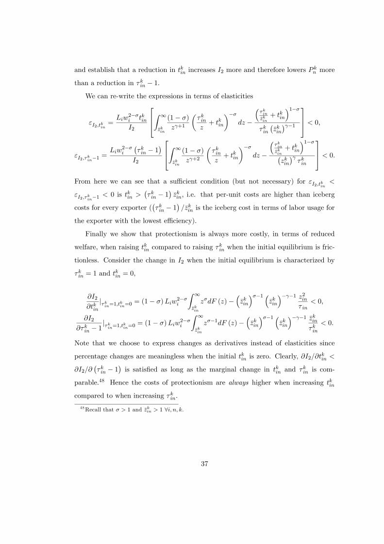
It is not possible to �nd a closed-form solution for the price index when tkin > 0.
However it is possible to study under which conditions the price index reacts more to
a change in per-unit trade costs than to a change in ad valorem trade costs. When
per-unit trade costs are initially high relative to ad valorem trade costs, the elasticity
of the price index with respect to a change in per-unit trade costs is higher than
with respect to a change in ad valorem trade costs. In the appendix we prove that
a su¢ cient (but not necessary) condition is tkin >��kin � 1
�=�zkin. The interpretation
of this condition is very intuitive: welfare is more sensitive to per-unit costs than
to ad valorem costs when per-unit costs are initially higher than ad valorem costs
(both expressed in terms of labor) for the least e¢ cient exporter. In the appendix we
also prove that the price index is always more sensitive to changes in per-unit costs
compared to changes in iceberg costs when the initial equilibrium is frictionless. We
summarize these �nding in the following two propositions:
Proposition 2 Consider an initial equilibrium with tkin > 0 and �kin > 1;8i; n; i 6= n.
The costs of trade protectionism in market n are higher, in terms of reduced welfare,
when raising tkin by 1 percent compared to when raising �kin by 1 percent, if t
kin >�
�kin � 1�=�zkin (su¢ cient condition).
Proof. See Appendix.
Proposition 3 Consider an initial frictionless equilibrium with tkin = 0 and �kin =
1;8i; n. The costs of trade protectionism in market n are always higher, in terms of
reduced welfare, when raising tkin compared to when raising �kin by a marginal amount.
Proof. See Appendix.
2.6 The Export Volume Distribution
In this section we examine some properties of the distribution of exports in a model
with per-unit costs. We will make extensive use of these properties later on when we
estimate trade costs. We �rst derive the theoretical export volume distribution for
every destination n and product k. Source country subscripts are dropped because
12
Norway is always the source in the data. Given that productivity among potential
entrants is distributed Pareto, the productivity distribution among exporters of prod-
uct k to destination n is also Pareto with CDF F�zj�zkn
�= 1�
�z=�zkn
�� . The Pareto
shape coe¢ cient is assumed to be equal across products and destinations. Then
the export volume CDF, conditional on z > �zkn, is15
Q�xj�zkn
�= Pr
hX < xjZ > �zkn
i= 1�
hAknx
�1=� �Bkni ; (3)
where Akn and Bkn are two clusters of parameters,
Akn =� � 1�
�zkn
�P kn
�(��1)=��1=�k
Y1=�n
�knw;
Bkn =tkn
�kn=zkn
:
2.6.1 Properties of the distribution
As with the scale parameter for the Pareto distribution, Akn will a¤ect the location of
the distribution. For example, an increase in market size Yn will shift the probability
density function to the right, so that it becomes more likely to sell bigger quantities.
Since Bkn = tkn=��kn=z
kn
�, Bkn simply measures per-unit trade costs (t
kn) relative to
the unit costs of the least e¢ cient �rm, inclusive ad-valorem costs (�kn=zkn). When
tkn = 0 =) Bkn = 0, the distribution is identical to Pareto with shape parameter
=�. This is similar to Chaney (2008) where the sales distribution preserves the shape
of the underlying e¢ ciency distribution and the sales distribution is identical across
markets. When tkn > 0, Bkn will a¤ect the dispersion of quantity sold. This can be
seen by �nding the inverse CDF:
xkn (�) = Q�1(�) =
"(1� �)1= +Bkn
Akn
#��:
15The CDF is well-behaved when�1+Bk
n
Akn
���� xkminn < 0 and xkmaxn �
�Bkn
Akn
���< 0 where xkminn
is the minimum export volume and xkmaxn is maximum export volume.
13
Dispersion, as measured by the ratio between the �th2 and �th1 percentiles (0 < �1 <
�2 < 1) is then
D��2; �1;B
kn; ; �
�� xkn (�2)
xkn (�1)=
"(1� �1)1= +Bkn(1� �2)1= +Bkn
#�: (4)
When tkn = 0, this ratio is constant across destinations. When tkn > 0, the ratio
declines as Bkn goes up. That is, export volume becomes less dispersed with higher
per-unit costs, controlling for the cuto¤ �zkn and �kn. The intuition is that higher per-
unit costs will hit the high productivity/low cost �rms harder than �rms with low
productivity/high cost, since more trade costs will force the high productivity �rms to
increase their price by more than the low productivity �rms, in percentage terms. This
will translate into a larger reduction in quantity sold for the high productivity �rms
relative to the low productivity �rms, so that dispersion will decrease. The following
proposition summarizes our �ndings:
Proposition 4 When per-unit costs are positive (tkin > 0), dispersion, as measured
by the ratio between the �th2 and �th1 percentiles, is decreasing in tkin and increasing in
�kin. Moreover, when per-unit costs are zero (tkin = 0), then dispersion is invariant to
a change in variable trade costs �kin.
Proof. See appendix.
In the appendix we prove this proposition allowing for trade costs to alter the
entry hurdles and the price index. The properties of the export volume distribution
also survive, under some assumptions, in a framework where �rms are heterogeneous
both in terms of unit costs and quality.16In the appendix we also investigate whether
departures from the CES framework can generate similar predictions as a model with
per-unit costs. We show that for a popular class of linear demand systems (and
16More speci�cally, the result that dispersion decreases with per unit costs carries through if high
price varieties sell less in terms of quantity than low price varieties. This occurs if unit costs are
negatively correlated with quality or if they are positively correlated up to a limit. Derivations are
available upon request. Johnson (2009) proposes a model where �rms are heterogeneous both in
terms of unit costs and quality.
14
with zero per-unit costs), dispersion in exports will increase in ad-valorem costs - the
opposite of the case with per-unit costs.
3 Estimating the model
In this section we structurally estimate the magnitude of per-unit trade costs. We saw
in the theory section that dispersion in export volume falls when per-unit trade costs
increase. When per-unit trade costs are zero, dispersion in export volume is una¤ected
by (ad valorem) trade costs. This is the identifying assumption that allows us to
recover estimates of trade costs consistent with our model.17 The econometric strategy
consists of using a minimum distance estimator that matches empirical dispersion in
export volume (per product-destination) to simulated dispersion in export volume.18
Our approach of estimating trade costs from an economic model is very di¤erent
from the previous literature.19 First, most studies model trade costs as ad valorem
exclusively, omitting the presence of per-unit costs. A notable exception is Hummels
and Skiba (2004), who distinguish between both and �nd evidence for the presence of
per-unit shipping costs.20 Compared to our work, they study freight costs exclusively,
whereas we consider all types of international trade costs. Second, our methodology
utilizes within-country dispersion in export volume to achieve identi�cation of trade
the traditional approach can only identify trade costs relative to some benchmark,
usually domestic trade costs, our method identi�es the absolute level of trade costs
(although conditional on a value of the elasticity of substitution).
17 In the data section below, we provide evidence that is consistent with the identifying assumption.18We choose to use data for export volume (quantities) instead of export sales for the following
reasons. First, a closed-form solution for the sales distribution does not exist. Second, using quantities
instead of sales avoids measurement error due to imperfect imputation of transport/insurance costs.
Third, we avoid transfer pricing issues when trade is intra-�rm (Bernard, Jensen and Schott 2006).19Anderson and van Wincoop (2004) provide a comprehensive summary of the literature.20They �nd an elasticity of freight rates with respect to price around 0:6, well below the unitary
elasticity implied by the iceberg assumption on shipping costs.
15
3.1 Data
The data consist of an exhaustive panel of Norwegian non-oil exports in the period
1996-2004.21 We observe export quantity and export value.22 Every export obser-
vation is associated with a �rm, destination and product id. The product ids are
based on the HS 8-digit nomenclature, and there are 5391 active HS8 products in the
data. 203 unique destinations are recorded in the dataset. Since identi�cation in the
empirical model is solely based on cross-sectional variation, we choose to work on the
2004 cross-section, the most recent available to us.
In 2004, 17; 480 �rms were exporting and total export value amounted to NOK 232
billion (� USD 34:4 billion), or 48 percent of aggregate manufacturing revenue. On
average, each �rm exported 5:6 products to 3:4 destinations for NOK 13:3 million (�
USD 2:0 million). On average, there are 3:0 �rms per product-destination (standard
deviation 7:8). As we will see, we will utilize the distribution of export quantity across
�rms within a product-destination in the econometric model. We therefore choose to
restrict the sample to product-destinations where more than 40 �rms are present.23
In the robustness section, we evaluate the e¤ect of this restriction by estimating the
model on di¤erent sets of destination-product pairs. In what follows, extreme values
of quantity sold, de�ned as values below the 1st percentile or above the 99th percentile
for every product-destination, are eliminated from the dataset. All in all, this brings
down the total number of products to 121 and the number of destinations to 21.24
Before presenting the formal econometric model, we show some descriptives that
suggest how dispersion is related to trade costs. In Figure 2, we �rst calculated
21Firm-product-year observations are recorded in the data as long as export value is NOK 1000 (�
USD 148) or higher.22The unit of measurement is kilos for 67:8% of the products, 27:5% are measured in quantities,
while 4:7% are measured in other units (m3, carat, etc.). The choice of unit depends on the product
characteristics.23Also, the likelihood function is relatively CPU intensive, and this restriction saves us a signi�cant
amount of processing time.24Exports to all possible combinations of these products and destinations amount to 26:2% of total
export value.
16
the ratio between the 90th and 10th percentile of export quantity for each product-
destination. Second, we averaged the ratios across products for every destination,
using export value for each product as weights.25 Third, we plotted the mean ratio
against distance, in logs. The relationship is clearly negative, indicating that trade
costs tend to narrow the dispersion in export quantity. Regressions that include the
usual gravity-type right hand side variables and product �xed e¤ects will give the
same result.26 The relationship is also robust to other measures of dispersion, such
as the Theil index or the coe¢ cient of variation.
The theoretical prediction of a negative correlation between per-unit trade costs
and export dispersion relies on the assertion that �rms in the top of the export
distribution charge lower prices than �rms in the bottom of the distribution. This
is something we can easily check in the data, as prices can be approximated by
unit values. In the data, we �nd that the average correlation between unit value
and (quantity) market share is �:32 (the average over all product-destinations). 84
percent of the correlations are negative.
3.2 Estimation
We use a minimum distance estimator that matches empirical dispersion in export
volume (per product-destination) to simulated dispersion in export volume. Speci�-
cally, denote the empirical ratio between the �th2 and �th1 percentiles for product k in
destination n as eDkn (�2; �1) and stack a set of (�2; �1) ratios in theM�1 column vec-
tor eDkn. Denote its simulated counterpart D
��2; �1;B
kn; ; �
�, as de�ned in equation
(4), and stack a set of (�2; �1) ratios in the M �1 column vector D�Bkn; ; �
�. De�ne
the criterion function as the squared di¤erence between lnD�Bkn; ; �
�and ln eDk
n:
d () =NXn
Xk2n
hlnD
�Bkn; ; �
�� ln eDk
n
i0 hlnD
�Bkn; ; �
�� ln eDk
n
i;
25 In order to show the pattern for as many destinations as possible, we have based these calculations
on the unrestricted sample, i.e. using all product-destinations with more than one �rm present.26Speci�cally, we regress the 90/10 percentile ratio on a product �xed e¤ect, distance, population
and real GDP per capita (all in logs), as well as contiguity.
17
where is the vector of coe¢ cients to be estimated, N is the total number of des-
tinations and n is the set of products sold in market n. We minimize d () with
respect to and denote b the equally weighted minimum distance estimator.27
We model Bkn as the product of sector and destination �xed e¤ects,
Bkn = �kbn;
and normalize �1 = 1.28 This decomposition enables us to identify the share of trade
costs that is due to product characteristics and the share that is due to market charac-
teristics. Also, note that even though �k is estimated relative to some normalization,
the estimates of the B�s are invariant to the choice of normalization. Finally, we
condition the criterion function on a guess of � (see next section). The coe¢ cient
vector then consists of = (�k; bn; ), in total K +N parameters.
We choose the following percentile ratio moments: (.95,.05), (.90,.10), (.75,.25),
Hence, we have M = 12 moments per product-destination.29
As the covariance matrix of the vector of empirical percentile ratios (ln ePkn) isunknown, the standard error of the estimator is not available using standard formu-
las. Instead, we employ a nonparametric bootstrap (empirical distribution function
bootstrap). Speci�cally, we sample with replacement within each product-destination
pair, obtaining the same number of observations as in the original sample. After per-
27Theory suggests that for overidenti�ed models it is best to use optimal GMM. In implementation,
however, the optimal GMM estimator may su¤er from �nit-sample bias (Altonji and Segal 1996).
Furthermore, it is di¢ cult to calculate the optimal weighting matrix in our context, as it would
necessitate evaluating the variance of the percentile ratios for every product-destination (see e.g.
Cameron and Trivedi section 6.7).28The normalization is similar to the one adopted in the estimation of two-way �xed e¤ects in the
employer-employee literature (see Abowd, Creecy and Kramarz 2002). We also need to ensure that
all products and destinations belong to the same mobility group. The intuition is that if a given
product is only sold in a destination where no other products are sold, then one cannot separate the
product from the destination e¤ect.29We experimented with other combinations of moments as well and the results remained largely
unchanged.
18
forming 500 bootstrap replications, we form the standard errors by calculating the
standard deviation for each coe¢ cient in .
3.3 Identi�cation
In Figure 3 we plot the inverse of the theoretical export volume CDF (1 � CDF ),
on log scales. 1 � CDF is on the horizontal axis, while quantity exported is on the
vertical axis. The solid line represents the case when Bkn = tkn=��kn=z
kn
�= 0. The
gradient is then equal to ��= . The dotted line represents the case when per-unit
costs are positive. As Bkn increases, 1 � CDF becomes more and more concave.
The set of percentile ratio moments enables us to trace out the curvature of the
CDF, which will pin down Bkn.30 The Pareto shape parameter is identi�ed by the
gradient of the CDF. Since is independent of product-destination (in the baseline
speci�cation), is identi�ed by the slope of the CDF that is common to all markets,
whereas Bkn is identi�ed by the curvature that is product-destination speci�c.31 The
economic interpretation is that the higher the per-unit costs (embedded in Bkn), the
less dispersion in export volume (captured by more concavity in 1� CDF ). As it is
usual in trade models, the elasticity of substitution � is not identi�ed. The criterion
function d () is therefore conditional on a guess of �. In the results section we report
estimates based on di¤erent values of �.
As already noted, Bkn = tkn=��kn=z
kn
�simply measures per-unit trade costs (tkn)
relative to the unit costs of the least e¢ cient �rm, inclusive ad-valorem costs (�kn=zkn).
A more common measure of trade costs is trade costs relative to price. First, using
the �rst order condition from the �rm�s maximization problem, we can re-express
30Note that with only one moment, Bkn and are not separately identi�ed, as one percentile ratio
will only give information about the slope of the CDF. Also note that a linear CDF (in logs) will
result in an estimate of zero per-unit trade costs.31A model with product-speci�c �s is also identi�ed. We estimate a model with heterogeneity in
and � in the robustness section.
19
�rm-level consumer prices can as
pkn(ez) = �wtkn� � 1
�1ezBkn + 1
�; (5)
where ez is productivity measured relative to the cuto¤ (z = ez�zkn).32 Second, considerthe average price of product k in destination n:
�pkn =
Z 1
1pkn (ez) dF �ezj�zkn = 1� :
Third, inserting equation (5) and solving for wtkn=�pkn yields:
wtkn�pkn
=
��
� � 1
Z 1
1
�1ezBkn + 1
�dF�ezj�zkn = 1���1 :
The ratio wtkn=�pkn measures (per-unit) trade costs relative to the average consumer
price. Given our estimate of Bkn and , the expression on the right hand side can be
computed. Note that integrating over productivities allows us to express trade costs
only as a function of Bkn, and �: This is due to the fact that a Pareto density is
parameterized only by the cuto¤ (�zkn) and the shape parameter ( ). Our estimates
of Bkn and are therefore su¢ cient to get a meaningful measure of per-unit trade
costs.33
3.4 Results
Table 1 summarizes the results.34 We apply the methodology described in the previous
section in order to back out a simple measure of per-unit costs from the model.
Estimated per-unit trade costs wtkn=�pkn, measured relative to the consumer price,
averaged over products and destinations, are 0:36 (s.e. 0:01), conditional on � = 6,
32Note that ~z is distributed like a Pareto with scale parameter 1.33 In the appendix, we consider an extension of our model, that departs from the standard CES
framework, where �rms have to sustain marketing costs in order to promote their products and reach
consumers, following Arkolakis (2008). It turns out that, in the extended model, as long as the market
penetration e¤ect is not too strong compared to the per-unit trade cost e¤ect, we can interpret our
results as a lower bound on the true magnitude of the ad-valorem equivalent of per-unit trade costs.34The estimates of �k and bn are available upon request.
20
which we use as our baseline case.35 Estimated trade costs drop to 0:35 for � = 4 and
rise to 0:45 for � = 8. These estimates are similar to the existing literature, where
international trade barriers are typically estimated in the range of 40�80 percent for
a 5� 10 elasticity estimate (Anderson and van Wincoop 2004).36
Furthermore, 99 and 95 percent of the �k and bn coe¢ cients respectively (the
product and destination �xed e¤ects embedded in Bkn) are signi�cantly di¤erent from
zero at the 0:05 level. Since Bkn is bigger than zero only when per-unit costs tkn > 0,
our �ndings suggest that the standard model with only iceberg costs is rejected.37
The estimate of , the Pareto coe¢ cient, is 1:31 (s.e. 0:03) in the baseline case.
Figure 4 shows wtkn=�pkn for every destination, averaged over products, on the ver-
tical axis and distance (in logs) on the horizontal axis (conditional on � = 6). Trade
costs are clearly increasing in distance. This mirrors the pattern we saw in Figure 2,
that dispersion is decreasing in distance. Note that our two-way �xed e¤ects approach
enables us to construct wtkn=�pkn even for product-destination pairs that are not present
in the data. This implies that there is no selection bias in Figure 4, since all products
are included in every destination. The robust relationship between distance and trade
costs also emerges when regressing trade costs on a product �xed e¤ect and a set of
gravity variables (distance, contiguity, GDP and GDP per capita, all in logs).38 The
distance coe¢ cient is then 0:07 (s.e. 0:001), meaning that doubling distance yields a
7% increase in trade costs.35� is estimated to 3:79 in Bernard, Eaton, Jensen and Kortum (2004). In summarizing the
literature, Anderson and van Wincoop (2004) conclude that � is likely to be in the range of �ve to
ten.36Previous estimates of international trade barriers are not directly comparable to our estimate of
wtkn=pkn, however, as previous studies de�ne trade barriers as the ratio of total (ad valorem) trade
barriers relative to domestic trade barriers � in=� ii.37We also test the hypothesis that all tkn = 0 formally. Let n be is the number of observations,
res
the vector of restricted coe¢ cients (all Bkn = 0) and unres the vector of unrestricted coe¢ cients.
Then the likelihood ratio statistic 2n [d (res;�)� d (unres;�)], is �2 (r) distributed under the null,
where r is the K + P � 1 restrictions. The null is rejected at any conventional p-values.38The full set of results is available upon request.
21
Figure 5 shows dispersion in trade costs from Norway to the U.S. across prod-
ucts (conditional on � = 6). This �gure essentially exploits the variability retrieved
from the �k variables. As expected, per-unit trade costs are heterogeneous, with val-
ues ranging from roughly 10 to 70 percent of the product value.39 Figure 6 shows
the relationship between estimated trade costs and actual average weight/unit and
weight/value in logs.40 Since weight/unit and weight/value should be positively cor-
related with actual trade costs, we expect to see a positive relationship between these
measures and estimated trade costs. Indeed, the �gures indicate an upward slop-
ing relationship. The correlation between weight/unit (weight/value) and trade costs
wtk=�pk (averaged over destinations) is 0:55 (0:38).
It is also of interest to study the importance of product and destination charac-
teristics on trade costs. Since the expression for wtkn=�pkn is a monotonically increasing
function of Bkn, a straightforward indicator of the importance of product and des-
tination characteristics is the dispersion in �k and bn respectively. In the baseline
case, the 90-10 percentile ratio of �k and bn is 5:40 and 1:63 respectively, suggesting
that product characteristics are 3� 4 times as important for trade costs compared to
destination characteristics.
Furthermore, the decomposition of product and destination e¤ects allows us to
study whether costly destinations are associated with products with lower transport
costs. Or in other words, that the product mix in a given destination is a selected
sample in�uenced by the costs of shipping to that market. A simple indicator is
the correlation between the destination �xed e¤ect bn and the product �xed e¤ect,
averaged over the products actually exported there. Formally, we correlate bn with
(1=Kn)Pk2n �k, where Kn is the number of products exported to destination n and
39Note that densities for other markets are simply shifted left or right compared to the density for
the U.S. This is by construction, since it is only the destination �xed e¤ect bn that is di¤erent in the
construction of the density for alternative markets.40Since only a subset of products has quantities measured in units, the number of products in
the graph is lower than what is used in the estimation. Average weight/unit and weight/value are
obtained by taking the unweighted average of these ratios (in logs) over �rms and destinations.
22
n is the set of products exported to n. The results indicate that there is not much
support for the hypothesis. The correlation is slightly positive but not signi�cantly
di¤erent from zero.
We also investigate whether the unweighted average of trade costs is di¤erent from
the weighted average.41 When using export values per product-destination as weights,
the weighted average of trade costs is 0:27. This suggests that product-destinations
associated with high costs have below average exports.
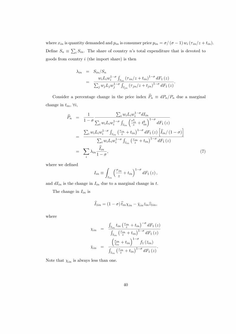
Finally, Figure 7 shows actual and simulated percentile ratios (95/05, 90/10, 75/25
and 60/40) (again conditional on � = 6), for all product-destination pairs. Most
observations lie close to the 45 degree line, although the �t of the model is declining
closer to the median. Overall, this leads us to conclude that the model is able to �t
the data quite well.
3.5 Robustness
A concern in the econometric model is our reliance on the Pareto distribution. Even
though the Pareto is known to approximate the US �rm size distribution quite well
(e.g. Luttmer 2007), one could argue that dispersion is decreasing with trade costs
due to extensive margin e¤ects. As is well known, the fractal nature of the Pareto
distribution implies that the 90/10 ratio is independent of truncation, implying the
entry hurdle does not a¤ect dispersion (when t = 0). However, under other distrib-
utions this is no longer the case. For example, with the lognormal distribution and
t = 0, dispersion will decrease with higher entry hurdles simply because the density is
truncated from below, not due to intensive margin reallocation. One way of control-
ling for this, is to examine dispersion for a subsample of �rms that exports a product
to many destinations, so that extensive margin e¤ects no longer operate. Speci�cally,
we take the 3 most popular destinations, Sweden, Denmark and Germany, and extract
the �rm-product pairs that are present in all three markets. This ensures that, for a
41We mainly focus on the unweighted average because otherwise we would have a selection problem
when comparing trade costs across destinations.
23
given product, the same set of �rms are present in all locations. We then estimate
the function pkn = �k+�1dn+�2yn+"kn, where pkn is the 90/10 percentile ratio, �k
is a product �xed e¤ect, dn is distance and yn is GDP (all in logs). Results are shown
in Table 2. Column (1) shows the coe¢ cients when the number of �rms present in a
given product-destination is 2 or more, while columns (2) and (3) show the coe¢ cients
when the threshold is 5 and 10 respectively. Even though we lose many observations
in this exercise, the results are reassuring. Dispersion is decreasing with distance even
among this balanced group of �rm-products. The distance coe¢ cient is signi�cant in
cases (1) and (2), but not in (3), where the number of products is reduced to 13.
Next we present some re-estimations of the model that address several issues. The
results are summarized in Table 3. First, a concern is that although the model pre-
sented in the theory section is about single-product �rms, our econometric approach
treats a multi-product �rm as several �rms producing di¤erent goods. We check the
importance of this approach by re-estimating the model on single-product �rms only.
Speci�cally, whenever multiple products are exported within a given �rm-destination
pair, this �rm-destination is deleted from the dataset. Naturally, this truncates the
data quite substantially, and we are left with only 8 destinations and 6 products (when
the product-destination cuto¤ is set to 40 �rms, as before). Nevertheless, the results
are reassuring. As shown in Table 3, column (R1), the grand mean of per-unit trade
costs is in this case 0:51 (conditional on � = 6).
Second, we investigate whether the choice of truncating the dataset to only product-
destinations with more than 40 �rms a¤ects the results. We choose product-destinations
with between 30 and 40 �rms present and re-estimate the model, resulting in 16 des-
tinations and 149 products. Again, the estimate of trade costs does not change much.
The grand mean is now 0:42, as shown in column (R2). Third, we investigate whether
the choice of units a¤ects the results. The high share of products that are measured
in kilos might bias the results if weight per-unit is varying across both destinations
and �rms. For example, if high productivity �rms are able to reduce unit weight in
remote markets, while low productivity �rms are not, then dispersion will decrease.
24
We address this issue by selecting the subsample of products that are measured in
units, not kilos. This truncates the dataset to 40 products and 6 markets. Again,
the results do not change much, as shown in column (R3) in the table. Fourth, we
re-estimate the model on the 2003 cross-section instead of the 2004 cross-section. The
results in column (R4) show that the grand mean of trade costs is identical to the
baseline result. Fifth, we estimate the model on a dataset of Portuguese exporters.
The data has the same structure as the Norwegian one. The results in column (R5)
show that mean per-unit trade costs for Portugal is 0:34, very close to the Norwegian
estimates (for � = 6).
We also check the sensitivity of the results to heterogeneity in the elasticity of
substitution � and the Pareto coe¢ cient . First, we take estimates of the � from
Broda and Weinstein (2006), and take the unweighted average of their HS 10 digit
estimates for every 4 digit product.42 Second, we allow for product-speci�c �s, so
that the theoretical percentile ratios become D��2; �1;B
kn; k; �k
�and the coe¢ cient
vector to be estimated becomes = (�k; bn; k), in total 2K+N�1 coe¢ cients. The
results are reported in column (R6). Again, per-unit costs are large and signi�cant,
although the point estimate falls somewhat compared to the baseline case.
Eaton, Kortum and Kramarz (2009) argue that sales and entry shocks are needed
in order to explain the entry and sales patterns of French exporters. Our model,
on the other hand has only variability along the productivity dimension. Although
additional error components would certainly increase the �t of the model, we decided
to choose a somewhat simpler setup in this paper.43 First, the de�ning feature of
the data we have attempted to explain is the varying dispersion in exports across
destinations. A model with entry and sales shocks but without per-unit costs cannot
explain this, unless one assumes that the variances and/or covariances of the shocks
are correlated with distance. Second, our econometric model is expressed in closed-
42We average up to the 4 digit level because i) only the �rst 6 digits are internationally comparable
and (ii) not all products are jointly present in the Norwegian and U.S. data.43 In a previous paper (Irarrazabal et al 2009) we estimated demand and �xed cost shocks in a
model with heterogeneous �rms, exports and horizontal FDI.
25
form, even though analytical expressions for many key relationships do not exist. This
helps to keep the run-time of the estimation program down to an acceptable level.44
4 Simulation: The costs of protectionism
In this section we explore how protectionism, or conversely trade liberalization, will
a¤ect welfare and aggregate TFP in the model. As we have seen previously, raising
per-unit costs will hit the most productive �rms harder than less productive �rms,
and this will have adverse e¤ects on the aggregate economy. The question here is how
strong this e¤ect is quantitatively. We solve three equilibria: (A) Frictionless trade,
where both � = 1 and t = 0, (B) Government must raise tari¤ revenue relative to total
import value (G=I)� through iceberg trade costs � > 1, and (C) Government must
raise (G=I)� through per-unit costs. To simplify the analysis, we focus on symmetric
two-country equilibria.45 We also remove some heterogeneity by focusing on a single
sector. Then, tkin = t and �kin = � for every k; i; n.
First, we need to decide on the target tari¤ revenue we want to obtain. We saw
in the previous section that the grand mean trade costs were 0:36 (conditional on
� = 6). Here we hypothesize that the government raises tari¤ revenues corresponding
to this level of trade costs, i.e. that tari¤ revenue relative to total c.i.f. imports is
(G=I)� = 0:36.
Second, we need to �nd the value of �� (in case B) and t� (in case C) that achieves
the target tari¤ revenue (G=I)�. In case (B), the answer is simply �� = 1:36.46 In case
(C) the problem is less trivial. Now tari¤ revenue per import observation is tx (z).
44Run-time on a dual Intel Xeon L5520 is approximately 350 seconds.45This implies that import tari¤s are retaliated: The foreign country also imposes tari¤s on home
country exports.46Tari¤ revenue in absolute terms is G =
P(� � 1) px = (� � 1) I, where the summation is over
every import observation, x is the quantity imported (the quantity that arrives) and p is the consumer
price (c.i.f). We assume that the government can convert the melted iceberg into cash by selling it
for the market price p.
26
Total tari¤ revenue is:
GC = wL
Zz(t)
tx (t; z) dF (z) : (6)
The problem then boils down to �nding the t� that yields�GC=I
��= 0:36. The
simulation consists of the following steps:
� First choose an initial value for t0 (close to 0), holding � = 1. Solve the equi-
librium and calculate tari¤ revenue (G=I)C0 according to (6).
� If���(G=I)� � (G=I)C0��� is su¢ ciently small, the tari¤ rate t� ((G=I)�) that gen-
erates tari¤ revenue (G=I)� is found. Otherwise, choose a slightly higher t1 and
repeat the previous step.
After obtaining t� we compute the equilibrium in case C and compare welfare in
all three cases, as measured by the inverse of the price index, and aggregate TFP,
de�ned as average productivity z, weighted by employment for each �rm.47
The other parameter values are summarized in Table 5 and are chosen as follows.
In our �rst set of simulations, we set � = 6 (elasticity of substitution), although we
check the results for other values of � as well (see the second and third parameter
sets in the table). The market size Y is normalized to 1e+ 5. Entry costs are chosen
so that all potential entrants enter the domestic market in equilibrium B, which is
equivalent to normalizing the home entry hurdle to 1 (for simplicity entry costs are
assumed to be the same in the domestic and the foreign market). Finally, the number
of potential entrants, which equals the number of random productivity draws, is set
so that the accuracy of the numerical approximation of the equilibrium is reasonably
high (1e+ 5).
There remains a numerical problem. The estimates of (the Pareto shape pa-
rameter) we found earlier were between 1:0 and 1:5, depending on the choice of �.
However, as is standard in a Chaney (2008) model, the price index is only de�ned
47Note that this is di¤erent from measured TFP, where calculations are typically based on sales,
instead of output (quantity).
27
when > ��1 (in our case this condition must hold when t = 0, i.e. in the frictionless
equilibrium). Therefore, we choose to simulate the model using the lowest possible
that gives us a well-de�ned equilibrium, = � � :99. We check the sensitivity of the
choice of as well (see the third parameter set in the table).
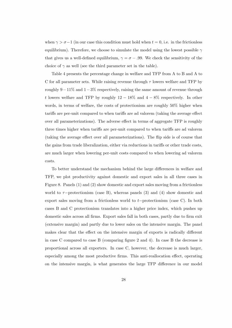
Table 4 presents the percentage change in welfare and TFP from A to B and A to
C for all parameter sets. While raising revenue through � lowers welfare and TFP by
roughly 9�11% and 1�3% respectively, raising the same amount of revenue through
t lowers welfare and TFP by roughly 12 � 18% and 4 � 8% respectively. In other
words, in terms of welfare, the costs of protectionism are roughly 50% higher when
tari¤s are per-unit compared to when tari¤s are ad valorem (taking the average e¤ect
over all parameterizations). The adverse e¤ect in terms of aggregate TFP is roughly
three times higher when tari¤s are per-unit compared to when tari¤s are ad valorem
(taking the average e¤ect over all parameterizations). The �ip side is of course that
the gains from trade liberalization, either via reductions in tari¤s or other trade costs,
are much larger when lowering per-unit costs compared to when lowering ad valorem
costs.
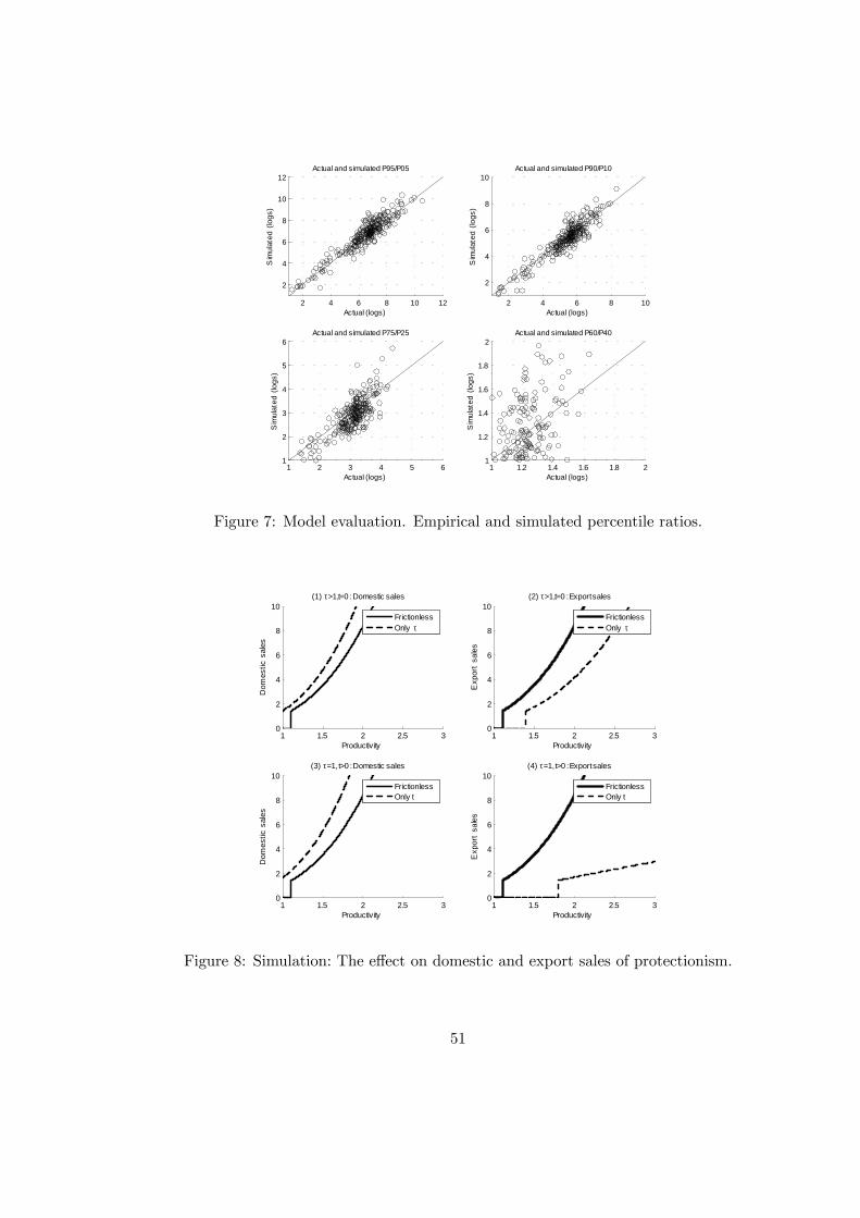
To better understand the mechanism behind the large di¤erences in welfare and
TFP, we plot productivity against domestic and export sales in all three cases in
Figure 8. Panels (1) and (2) show domestic and export sales moving from a frictionless
world to ��protectionism (case B), whereas panels (3) and (4) show domestic and
export sales moving from a frictionless world to t�protectionism (case C). In both
cases B and C protectionism translates into a higher price index, which pushes up
domestic sales across all �rms. Export sales fall in both cases, partly due to �rm exit
(extensive margin) and partly due to lower sales on the intensive margin. The panel
makes clear that the e¤ect on the intensive margin of exports is radically di¤erent
in case C compared to case B (comparing �gure 2 and 4). In case B the decrease is
proportional across all exporters. In case C, however, the decrease is much larger,
especially among the most productive �rms. This anti-reallocation e¤ect, operating
on the intensive margin, is what generates the large TFP di¤erence in our model
28
compared to the standard ad valorem case.
5 Conclusions
In this paper we have �rst explored theoretically the implications of introducing more
�exible trade costs in an otherwise standard Melitz (2003) heterogeneous �rm model
of international trade. An important �nding is that we identify an additional channel
of gains from trade through intensive margin reallocation compared to the standard
model. The mechanism behind the result is that the more productive �rms are hit
harder by trade costs compared to the less productive �rms when trade costs are
independent of e¢ ciency (and price). It is thus the marriage of per-unit costs and
heterogeneity in e¢ ciency that drives the theoretical results in this paper.
We tie the stylized model to a rich �rm-level dataset of exports, by product and
destination. By using the identifying assumption from theory that within product-
destination dispersion in export quantity will fall when (per-unit) trade costs are high,
we are able to back out a structural estimate of trade costs. Our empirical results
indicate that per-unit costs are not just a theoretical possibility: They are pervasive in
the data, and the grand mean of trade costs, expressed relative to the consumer price,
is between 35% and 45%, depending on the elasticity of substitution. We therefore
conclude that pure iceberg is rejected at the product level, and that empirical work
at this level of disaggregation must account for both the tip of the iceberg, as well as
the part of trade costs that are largely hidden under the surface: per-unit costs.
A broader implication of our work is related to the skill premium. To the extent
that more productive �rms demand more high-skill labor (e.g. as in Verhoogen 2008),
lowering trade barriers will increase aggregate demand for high skill labor through the
intensive margin reallocation channel emphasized in this paper. As a consequence,
our model makes clear an additional link between trade (the decline in international
transportation costs) and the skill premium.
Finally, we explore the welfare implications of protectionism by calibrating the
29
model with plausible parameter values. First, we ask what are the costs, in terms of
welfare and aggregate TFP, by moving from a frictionless economy to an equilibrium
with only iceberg tari¤s. Second, we calculate the same costs when moving from a
frictionless world to an equilibrium with only per-unit tari¤s. It turns out that the
intensive margin channel of reallocation induced by per-unit costs is not just a tech-
nical matter. The welfare costs are 50% higher when protecting with per-unit tari¤s
compared to protecting with iceberg tari¤s. The costs in terms of aggregate TFP loss
are about three times as high. All in all, this suggests that existing estimates of the
potential for gains from trade may be too low, and furthermore that the potential for
productivity growth induced by trade liberalization may be considerably larger than
previously thought. A fairly robust policy implication of our work is therefore that, if
governments are determined to raise revenue through import duties, they should im-
pose ad valorem duties rather than per-unit duties, due to the additional distortions
associated with per-unit duties.
30
References
[1] John M. Abowd & Robert H. Creecy & Francis Kramarz. 2002. "Computing
Person and Firm E¤ects Using Linked Longitudinal Employer-Employee Data,"
Working paper
[2] Alchian, Armen A., and William R. Allen. 1964. University Economics. Belmont,
Calif.: Wadsworth
[3] Altonji and Segal. 1996. "Small-Sample Bias in GMM Estimation of Covariance
Structures," Journal of Business & Economic Statistics, Vol. 14, No. 3, pp. 353-
366
[4] Anderson, James E., van Wincoop, Eric. 2003. "Gravity with Gravitas: A Solu-
tion to the Border Puzzle," American Economic Review, Volume 93, Issue 1, pp.
170-192
[5] Anderson, James E., van Wincoop, Eric. 2004. "Trade Costs," Journal of Eco-
nomic Literature, Volume 42, Number 3, 1 September 2004 , pp. 691-751(61)
[6] Arkolakis, K., (2008) "Market Penetration Costs and the New Consumers Margin
in International Trade", mimeo Yale University.
[7] Arkolakis, K., Costinot, A. and A. Rodríguez-Clare. 2009. "New Theories, Same
Old Gains?," Working paper
[8] Berman, N., Martin, P. and T. Mayer. 2009 "How Do Di¤erent Exporters React
to Exchange Rate Changes? Theory, Empirics and Aggregate Implications."
Manuscript.
[9] Bernard, A., Jensen, B. and P. Schott. 2006. "Transfer Pricing by US-Based
Multinational Firms." NBER Working Paper 12493
[10] C. Broda and D. Weinstein. 2006. "Globalization and the Gains from Variety,"
Quarterly Journal of Economics, Volume 121, Issue 2
31
[11] Cameron A.C. and P. K. Trivedi. 2005. Microeconometrics: Methods and Appli-
cations. Cambridge University Press.
[12] Christian Broda & David Weinstein, 2006."Globalization and the gains from