The Transportation FutureProject: Planning for Technology Change

David Levinson, Principal InvestigatorDepartment of Civil, Environmental and Geo- Engineering

University of Minnesota

January 2016

Research ProjectFinal Report 2016-02

s

To request this document in an alternative format call 651-366-4718 or 1-800-657-3774 (Greater Minnesota) or email your request to ADArequest.dot@state.mn.us. Please request at least one week in advance.

Technical Report Documentation Page 1. Report No. 2. 3. Recipients Accession No. MN/RC 2016-02 4. Title and Subtitle 5. Report Date

The Transportation Futures Project: Planning for Technology Change

January 2016 6.

7. Author(s) 8. Performing Organization Report No. David Levinson, Adam Boies, Jason Cao, Yingling Fan 9. Performing Organization Name and Address 10. Project/Task/Work Unit No. University of Minnesota Dept. of Civil, Environmental, and Geo- Engineering 500 Pillsbury Drive S.E. Minneapolis, MN 55455

University of Minnesota Humphrey School of Public Affairs 301 19th Avenue S Minneapolis, MN 55455

CTS #2016002 11. Contract (C) or Grant (G) No.

(c) 99008 (wo) 192

12. Sponsoring Organization Name and Address 13. Type of Report and Period Covered Minnesota Department of Transportation Research Services & Library 395 John Ireland Boulevard, MS 330 St. Paul, Minnesota 55155-1899

Final Report 14. Sponsoring Agency Code

15. Supplementary Notes http://www.lrrb.org/pdf/201602.pdf 16. Abstract (Limit: 250 words)

After a long period of system deployment of the auto-highway system, and several decades of maturity of that system, the surface transportation sector is facing a large number of technological shifts that could change whether and how people travel. While nascent, their prospects are potentially significant. This research proposed to explore these technologies - ascertain their potential market, consider their interactions, understand what that might do to travel demands, and address how planning and forecasting should respond. This research developed a series of white papers: high-level policy briefs based on our analysis of each technology, its direction, and its implications for Minnesota. This work extends and complements the MnDOT 50 year vision expressed in Minnesota GO. It also builds on the ideas developed in the NCHRP 750 project: Strategic Issues Facing Transportation. The timeframe on these technologies varies, and the authors looked at deployment paths over time rather than simple snapshots in time.

17. Document Analysis/Descriptors 18. Availability Statement forecasting, technological forecasting, travel demand, technological innovations, planning

No restrictions. Document available from: National Technical Information Services, Alexandria, Virginia 22312

19. Security Class (this report) 20. Security Class (this page) 21. No. of Pages 22. Price Unclassified Unclassified 141

The Transportation Futures Project: Planning for Technology Change

Final Report

Prepared by: David Levinson

Adam Boies Department of Civil, Environmental and Geo- Engineering

University of Minnesota

Jason Cao

Yingling Fan Humphrey School of Public Affairs

University of Minnesota

January 2016

Published by: Minnesota Department of Transportation

Research Services & Library 395 John Ireland Boulevard, MS 330

St. Paul, Minnesota 55155-1899

This report represents the results of research conducted by the authors and does not necessarily represent the views or policies of the Minnesota Department of Transportation or the University of Minnesota. This report does not contain a standard or specified technique.

The authors, the Minnesota Department of Transportation and the University of Minnesota do not endorse products or manufacturers. Trade or manufacturers’ names appear herein solely because they are considered essential to this report.

Table of Contents

Chaper 1: Autonomous Vehicles ........................................................................................................ 1

1.1 Connected vs. Autonomous Vehicles .................................................................................. 5

1.2 Timeline ............................................................................................................................... 6

1.3 Environments ....................................................................................................................... 7

1.4 Consequences ....................................................................................................................... 8

1.5 The Future of Travel Demand and Where We Live: The Out Scenario ............................ 12

1.6 Discussion .......................................................................................................................... 13

1.7 Consequences ..................................................................................................................... 14

Chaper 2: Mobile Telecommunications and Activity In-Motion ..................................................... 16

2.1 Introduction ........................................................................................................................ 16

2.2 Existing Empirical Evidence .............................................................................................. 16

2.3 Identification of New Activities in-Motion Using ATUS Data ......................................... 19

2.4 Impacts of the New Technologies ...................................................................................... 21

Chaper 3: Information and Communication Technologies .............................................................. 24

3.1 Introduction ........................................................................................................................ 24

3.2 Telecommuting .................................................................................................................. 24

3.2.1 The impacts of telecommuting on transportation ....................................................... 24

3.2.2 Trend analysis ............................................................................................................. 25

3.2.3 Perspective .................................................................................................................. 28

3.3 E-shopping ......................................................................................................................... 29

3.3.1 The impacts of e-shopping on transportation ............................................................. 29

3.3.2 Trend analysis ............................................................................................................. 31

3.3.3 Perspectives ................................................................................................................ 32

3.4 Other Tele-activities and Travel ........................................................................................ 32

3.5 Summary of ICT and travel ............................................................................................... 33

Chaper 4: Mobility-as-a-Service ...................................................................................................... 36

4.1 Sharing Cars ....................................................................................................................... 36

4.2 Sharing Rides ..................................................................................................................... 39

4.3 Sharing Bikes ..................................................................................................................... 41

4.4 The Future of Sharing: Cloud Commuting ........................................................................ 44

4.5 The Future of Travel Demand and Where We Live: The Up Scenario ............................. 47

4.6 Discussion .......................................................................................................................... 48

Chaper 5: Quantified Self and Quantified Networks........................................................................ 50

5.1 Introduction ........................................................................................................................ 50

5.2 Smartphone-Based Mobility Sensing and Quantification Apps ........................................ 50

5.3 Quantified Self and the Potential of Travel Behavior Intervention ................................... 53

5.4 Discussion on Quantified Self and Quantified Networks .................................................. 54

Chaper 6: Electrification and Alternative Fuels ............................................................................... 56

6.1 Introduction ........................................................................................................................ 56

6.2 Alternative Fuel Vehicle Trends ........................................................................................ 57

6.3 Drop-in Biofuels ................................................................................................................ 57

6.4 Electric Vehicles ................................................................................................................ 61

6.4.1 Powering Electric Vehicles ........................................................................................ 63

6.4.2 Electric Vehicle Penetration ....................................................................................... 64

6.4.3 Dynamic Wireless Power Transfer ............................................................................. 65

6.5 Natural Gas ........................................................................................................................ 67

6.6 Other Fuel Alternatives ...................................................................................................... 68

6.7 Fuel Tax Revenue .............................................................................................................. 68

6.8 Vehicle Mass ...................................................................................................................... 69

6.9 Conclusion and Discussion ................................................................................................ 71

Chaper 7: Road Pricing ..................................................................................................................... 73

7.1 Introduction ........................................................................................................................ 73

7.2 Toll Roads .......................................................................................................................... 75

7.3 Toll Areas........................................................................................................................... 78

7.4 Toll Lanes .......................................................................................................................... 78

7.5 Truck-only Toll Lanes ....................................................................................................... 80

7.6 Mileage Charges ................................................................................................................ 81

Chaper 8: New Logistics .................................................................................................................. 86

8.1 Introduction ........................................................................................................................ 86

8.2 Logistics Organization ....................................................................................................... 88

8.2.1 Supply Chain Network Pooling .................................................................................. 89

8.2.2 Physical Internet ......................................................................................................... 89

8.3 Business Delivery .............................................................................................................. 91

8.3.1 Business-to-business ................................................................................................... 91

8.3.2 Same Day Delivery ..................................................................................................... 92

8.4 Home Delivery ................................................................................................................... 92

8.4.1 Same Day Delivery ..................................................................................................... 92

8.5 Atoms into Bits .................................................................................................................. 97

8.5.1 Consolidated Home Delivery ................................................................................... 100

8.6 S-Curves ........................................................................................................................... 100

References ...................................................................................................................................... 105

Appendix A: Logistic Growth Curve Analysis

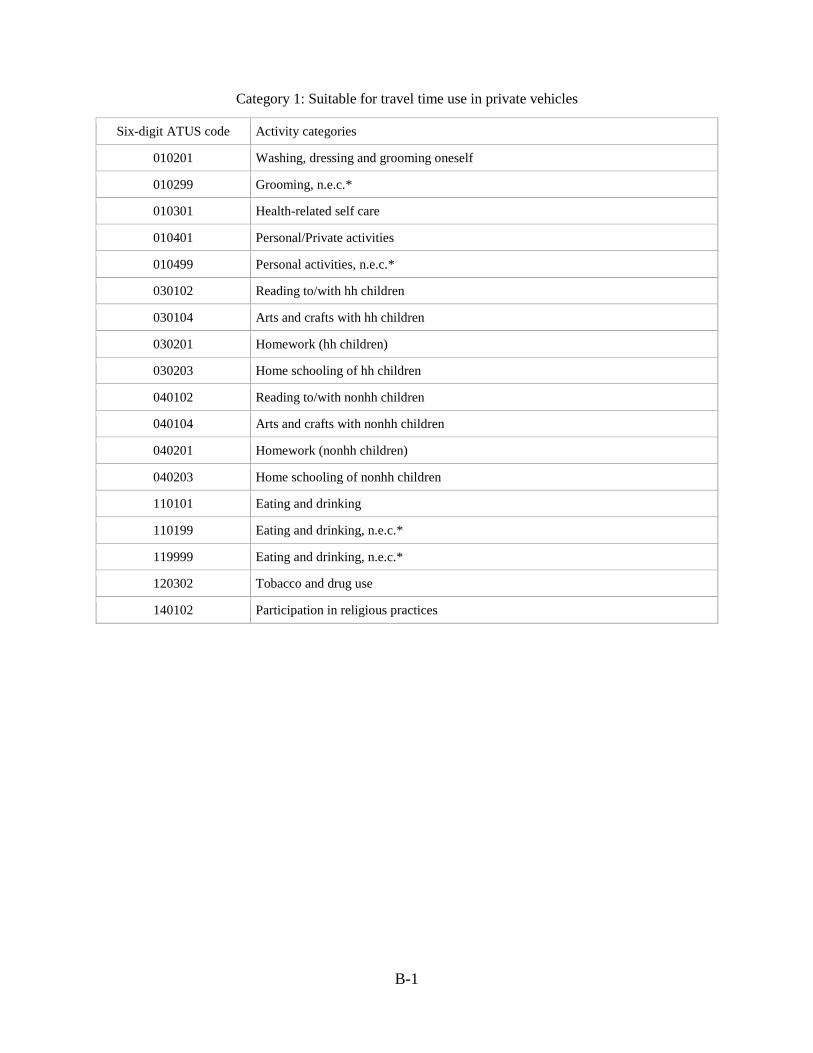
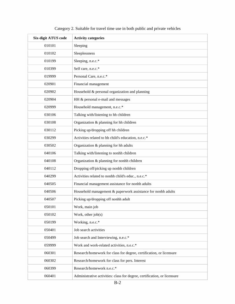
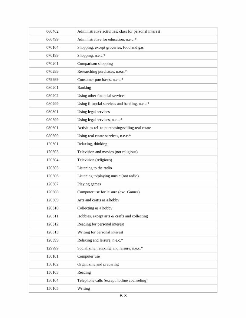
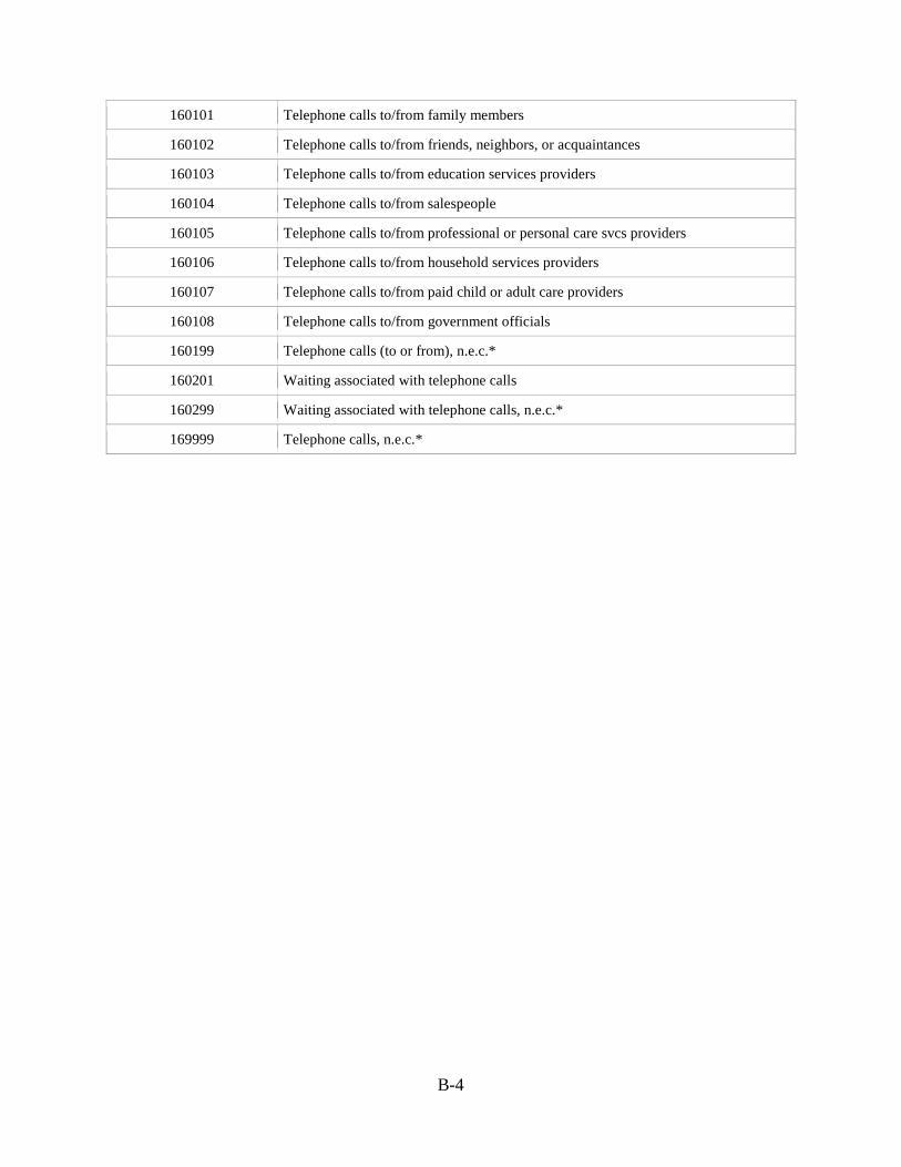
Appendix B: ATUS activity codes categorized by suitability for travel time use in the era of self-driving cars and better mobile technologies

Appendix C: Logistic Growth Curve Analysis

Appendix D: Logistic Growth Curve Analysis

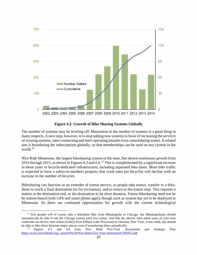
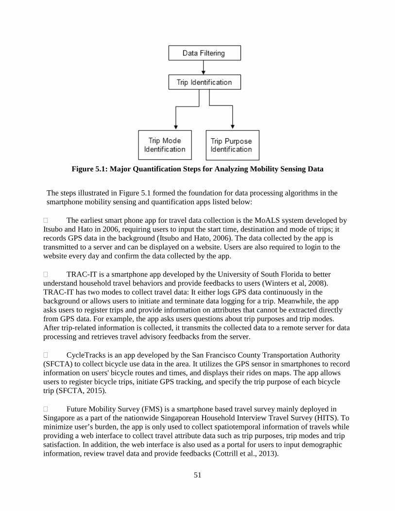
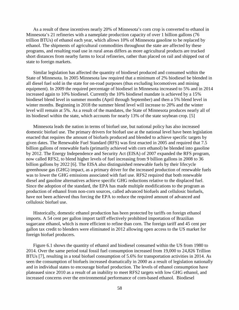
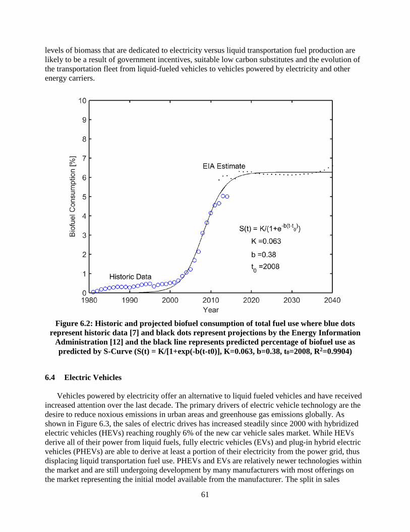
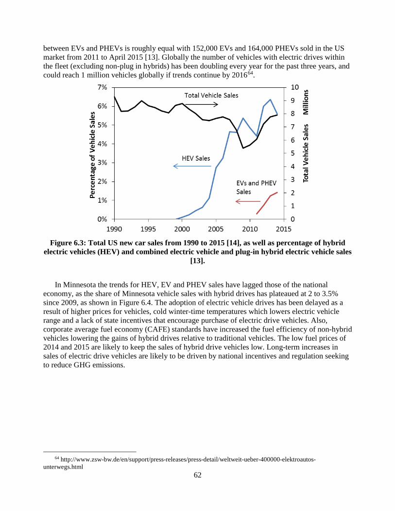
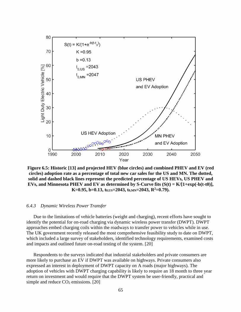
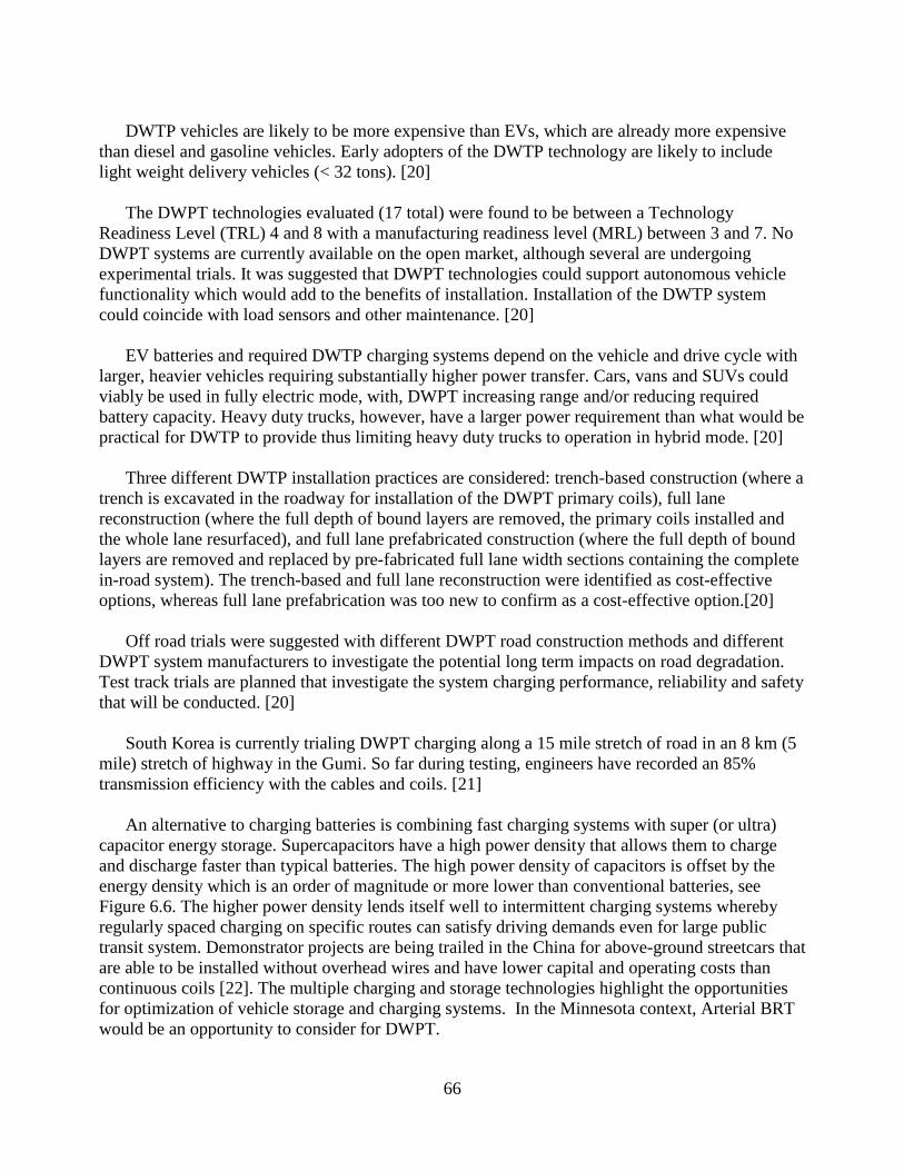
List of Figures Figure 1.1: Tesla Model S with Autopilot (a) Exterior (b) Interior. ................................................... 3 Figure 1.2: Cumulative miles traveled by Google Autonomous Vehicles .......................................... 4 Figure 1.3: US New Car Market by NHTSA Automation Level (author estimates) ......................... 6 Figure 1.4: US Vehicle Fleet by NHTSA Automation Level............................................................. 6 Figure 2.1: Activities most frequency studied as activities during travel ........................................ 18 Figure 2.2: Potential Drivers of Transit Ridership by Age (Figure downloaded from Transit Center, 2014) ................................................................................................................................................. 19 Figure 2.3: Average daily time spent on the identified new activities based upon 2011-2014 ATUS. .......................................................................................................................................................... 21 Figure 2.4: Picture (left) showing a prototype self-driving car and picture (right) showing Toyota Swagger Wagon Supreme as an example of demand for more activity options in private cars. ..... 22 Figure 2.5: Illustrative frequency distribution of “utility” of travel time by mode (adapted based upon Lyons and Urry, 2005)............................................................................................................. 22 Figure 2.6: A two-step hypothesis on the implications of mobile technology for spatial behavior. Step 1: circular trips replace hub-and-spoke trips to and from a point of gravity; Step 2: the number of trips increases (and/or chosen destinations for existing trips change) due to increased efficiency and information. (Figure downloaded from Dal Fiore et al, 2014) .................................................. 23 Figure 3.1: The Share of Work-at-Home Workers in Workforce .................................................... 27 Figure 3.2: The Share of E-commerce in Total Retail Sales ............................................................ 31 Figure 4.1: North American Carsharing Growth .............................................................................. 38 Figure 4.2: Growth of Bike Sharing Systems Globally .................................................................... 43 Figure 4.3: NiceRide’s Service Area continues to grow (source NiceRide MN, 2015) ................... 44 Figure 4.4: NiceRide’s Annual Revenue continues to grow (source NiceRide MN, 2015) ............. 45 Figure 5.1: Major Quantification Steps for Analyzing Mobility Sensing Data................................ 51 Figure 6.1: U.S. ethanol (top) and biodiesel (bottom) consumption from 1995 to 2014 (solid lines) [7] and proposed and revised biofuel production mandated by the Renewable Fuel Standard 2nd Implementation [10] and revised by the EPA in 2014 [11]. ............................................................. 60 Figure 6.2: Historic and projected biofuel consumption of total fuel use where blue dots represent historic data [7] and black dots represent projections by the Energy Information Administration [12] and the black line represents predicted percentage of biofuel use as predicted by S-Curve (S(t) = K/[1+exp(-b(t-t0)], K=0.063, b=0.38, t0=2008, R2=0.9904) ......................................................... 61 Figure 6.3: Total US new car sales from 1990 to 2015 [14], as well as percentage of hybrid electric vehicles (HEV) and combined electric vehicle and plug-in hybrid electric vehicle sales [13]. ....... 62 Figure 6.4: New car sales and percentage of vehicles with electric drives (HEVs, PHEVs and EVs) in Minnesota from 2008 to 2014 [15]. .............................................................................................. 63 Figure 6.5: Historic [13] and projected HEV (blue circles) and combined PHEV and EV (red circles) adoption rate as a percentage of total new car sales for the US and MN. The dotted, solid and dashed black lines represent the predicted percentage of US HEVs, US PHEV and EVs, and Minnesota PHEV and EV as determined by S-Curve fits (S(t) = K/[1+exp(-b(t-t0)], K=0.95, b=0.13, t0,US=2043, t0,MN=2043, R2=0.79). ....................................................................................... 65 Figure 6.6: Energy and power density of energy storage technologies that can be supplied to vehicles. [23] .................................................................................................................................... 67 Figure 6.7: Natural gas portion of heavy duty fuel use projection from 2012 to 2040 [28]. ........... 68 Figure 6.8: Change in adjusted fuel economy, weight and horsepower from model year 1975 to 2014. [35].......................................................................................................................................... 70

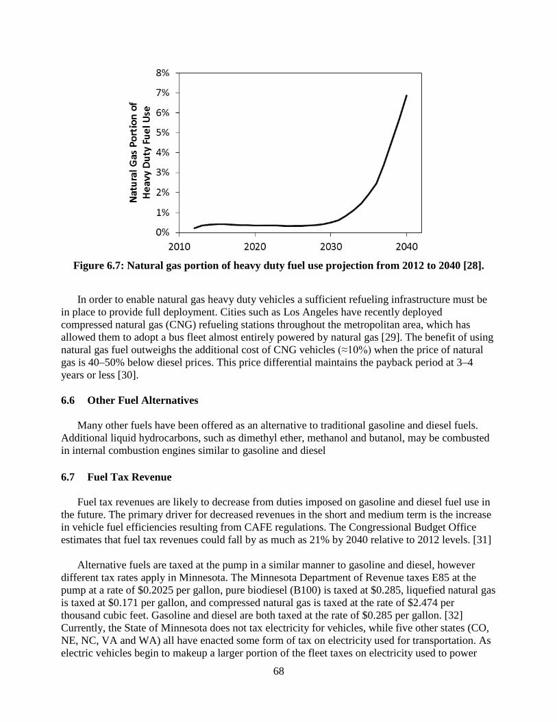
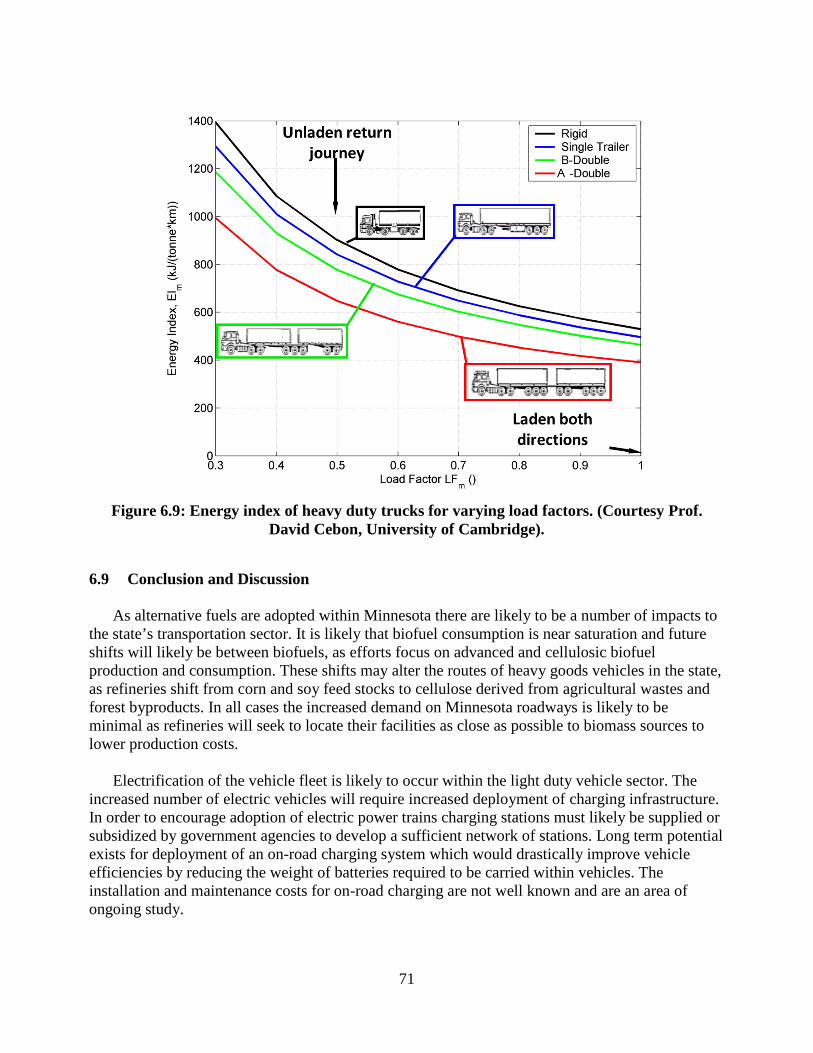
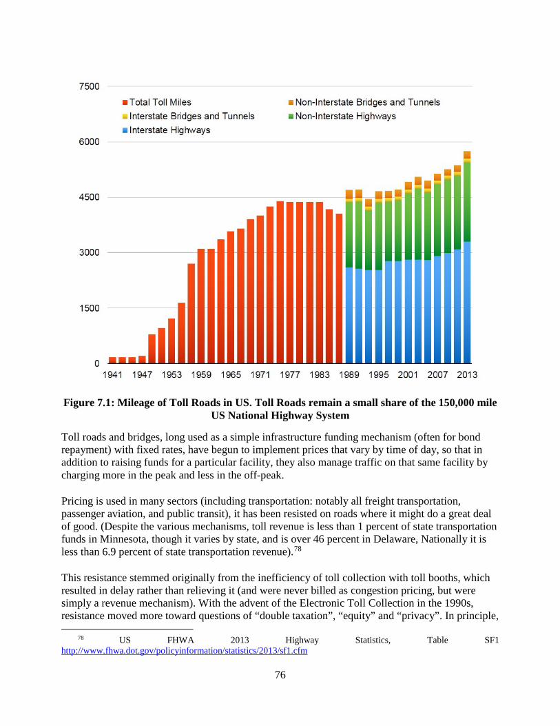
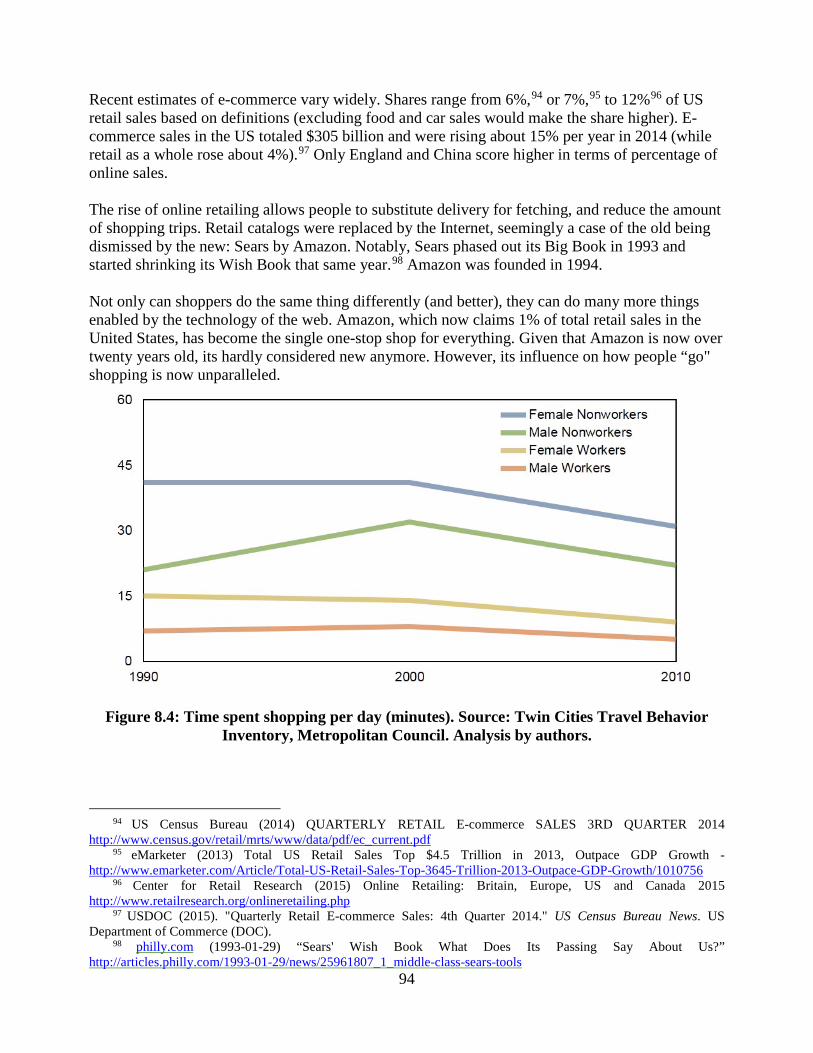
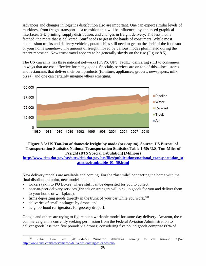
Figure 6.9: Energy index of heavy duty trucks for varying load factors. (Courtesy Prof. David Cebon, University of Cambridge). ................................................................................................... 71 Figure 7.1: Mileage of Toll Roads in US. Toll Roads remain a small share of the 150,000 mile US National Highway System ................................................................................................................ 76 Figure 7.2: Lane Miles of High Occupancy/Toll Lanes in United States ........................................ 80 Figure 8.1: Seasonally-adjusted truck tonnage on US road network from 2000 to 2015. [3] .......... 87 Figure 8.2: MN motor fuel tax revenue for 1980 to 2014. ............................................................... 88 Figure 8.3: Same-day delivery merchandise value and shipping fees generated in the United States from 2013 to 2018 (in billion US dollars) [15] ................................................................................ 93 Figure 8.4: Time spent shopping per day (minutes). Source: Twin Cities Travel Behavior Inventory, Metropolitan Council. Analysis by authors. ................................................................... 94 Figure 8.5: US Ton-km of domestic freight by mode (per capita). Source: US Bureau of Transportation Statistics National Transportation Statistics Table 1-50: U.S. Ton-Miles of Freight (BTS Special Tabulation) (Millions) ................................................................................................ 96 Figure 8.6: US home entertainment revenue (2013 $B). Source: Wall Street Journal and Digital Entertainment Group Fritz, Ben (2014) Sales of Digital Movies Surge. Wall Street Journal. 2014-01-07 http://www.wsj.com/news/articles/SB10001424052702304887104579306440621142958 . 98 Figure 8.7: US freight deliveries where the blue dots represent historic data and black line represents predicted future freight deliveries by S-Curve (S(t) = K/[1+exp(-b(t-t0)], K=8×106, b=0.035, t0=1980). Source: Data in this table are improved estimates based on the Freight Analysis Framework (FAF). Technical Summary of Updated Methodology is available at http://www.rita.dot.gov/bts/sites/rita.dot.gov.bts/files/FreightTonMilesMethodology.pdf ........... 101 Figure 8.8: European adoption of supply chain networking as a percentage of freight movements where pooling could fill loads that are not already at maximum mass or volume capacity. The blue dots represent expert responses to surveys and black line represents predicted percentage of synchronized consolidation as predicted by S-Curve (S(t) = K/[1+exp(-b(t-t0)], K=0.5, b=0.7739, t0=2017, R2=0.8462). ...................................................................................................................... 102 Figure 8.9: Adoption of urban consolidation where the blue dots represent expert responses to surveys and black line represents predicted percentage of synchronized consolidation as predicted by S-Curve (S(t) = K/[1+exp(-b(t-t0)], K=0.5, b=0.7739, t0=2017, R2=0.8462). .......................... 103

List of Tables Table 2.1: Summary of activities undertaken during travel in existing studies ............................... 17 Table 6.1: Ethanol and biodiesel yield per acre from selected crops. [9] ......................................... 59

Executive Summary The next two decades will see more change in the transportation sector than have been seen in 100 years. The introduction of autonomous vehicles, from a few cars initially, to all new cars, to eventually all cars will radically change how transportation is used. The concomitant electrification of vehicles will provide further opportunities to better optimize the use of transportation systems. Finally, continuing advances in information and mobile communications technology will up-end the way people think about transportation systems. This report explores in eight chapters the changes that are coming. Fully autonomous test vehicles from automakers and new entrants like Google have traveled in general traffic over 1 million miles collectively. Semi-autonomous vehicles are already here. Tesla auto-pilot (available in about 100,000 cars), for instance, can both keep lanes and follow the car in front, in addition to automatically changing lanes with direction from the driver. Tesla cars drive over 1 million miles per day nationally, though the amount of that in semi-autonomous mode is proprietary. The transition from human driven vehicles to fully autonomous vehicles is tricky. Some automakers believe that incremental transition is viable. Others note the danger of semi-autonomous vehicles that require periodic human intervention, and argue instead for step-jump to fully autonomous vehicles. The impacts described below are associated with fully autonomous vehicles (no driver control). We anticipate the following timeline for the deployment of fully autonomous vehicles (chapter 1):

• 2020 market availability, • 2030 regulatory requirement for all new cars, • 2040 prohibition of non-autonomous vehicles from public roads at most times.

The consequences of fully autonomous vehicles are numerous. Some of the more important ones are listed below and discussed more fully in the report.

• Increased safety overall as driverless cars don’t get tired and have better sensors and algorithms than humans. If driverless cars are not significantly safer, they will not be permitted. Total fatalities may drop over 90% with driverless vehicles as human error is eliminated. No system can be perfectly safe, but it will be significantly safer. Road designs and sight-lines will be far less relevant than design criteria as a result.

• An explosion of vehicle forms, including new, narrow, single-passenger vehicles, which will be safer than motorcycles given their automated drivers and new structural designs enabled by electrification. People will feel more comfortable in small vehicles mixed with large vehicles if all are automated.

• Increased capacity from existing pavements as cars can follow with a shorter headway and can occupy narrower lanes. This implies far more capacity in existing lanes, and less need to expand roads.

• Higher speeds on limited access roadways, as driver comfort with car-following and speed is no longer determinative of the maximum speed of travel.

• Lower speeds on local streets as automated vehicles better obey traffic laws and slow down to avoid collisions with other road users like pedestrians and bicyclists.

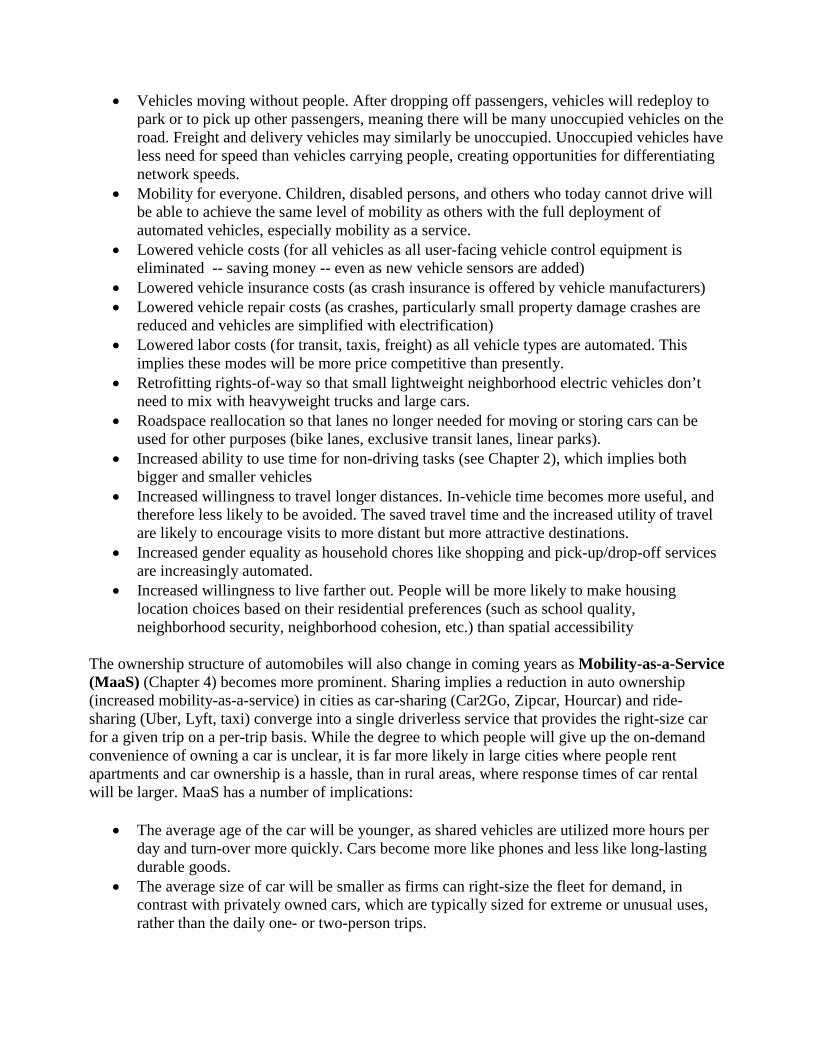
• Vehicles moving without people. After dropping off passengers, vehicles will redeploy to park or to pick up other passengers, meaning there will be many unoccupied vehicles on the road. Freight and delivery vehicles may similarly be unoccupied. Unoccupied vehicles have less need for speed than vehicles carrying people, creating opportunities for differentiating network speeds.

• Mobility for everyone. Children, disabled persons, and others who today cannot drive will be able to achieve the same level of mobility as others with the full deployment of automated vehicles, especially mobility as a service.

• Lowered vehicle costs (for all vehicles as all user-facing vehicle control equipment is eliminated -- saving money -- even as new vehicle sensors are added)

• Lowered vehicle insurance costs (as crash insurance is offered by vehicle manufacturers) • Lowered vehicle repair costs (as crashes, particularly small property damage crashes are

reduced and vehicles are simplified with electrification) • Lowered labor costs (for transit, taxis, freight) as all vehicle types are automated. This

implies these modes will be more price competitive than presently. • Retrofitting rights-of-way so that small lightweight neighborhood electric vehicles don’t

need to mix with heavyweight trucks and large cars. • Roadspace reallocation so that lanes no longer needed for moving or storing cars can be

used for other purposes (bike lanes, exclusive transit lanes, linear parks). • Increased ability to use time for non-driving tasks (see Chapter 2), which implies both

bigger and smaller vehicles • Increased willingness to travel longer distances. In-vehicle time becomes more useful, and

therefore less likely to be avoided. The saved travel time and the increased utility of travel are likely to encourage visits to more distant but more attractive destinations.

• Increased gender equality as household chores like shopping and pick-up/drop-off services are increasingly automated.

• Increased willingness to live farther out. People will be more likely to make housing location choices based on their residential preferences (such as school quality, neighborhood security, neighborhood cohesion, etc.) than spatial accessibility

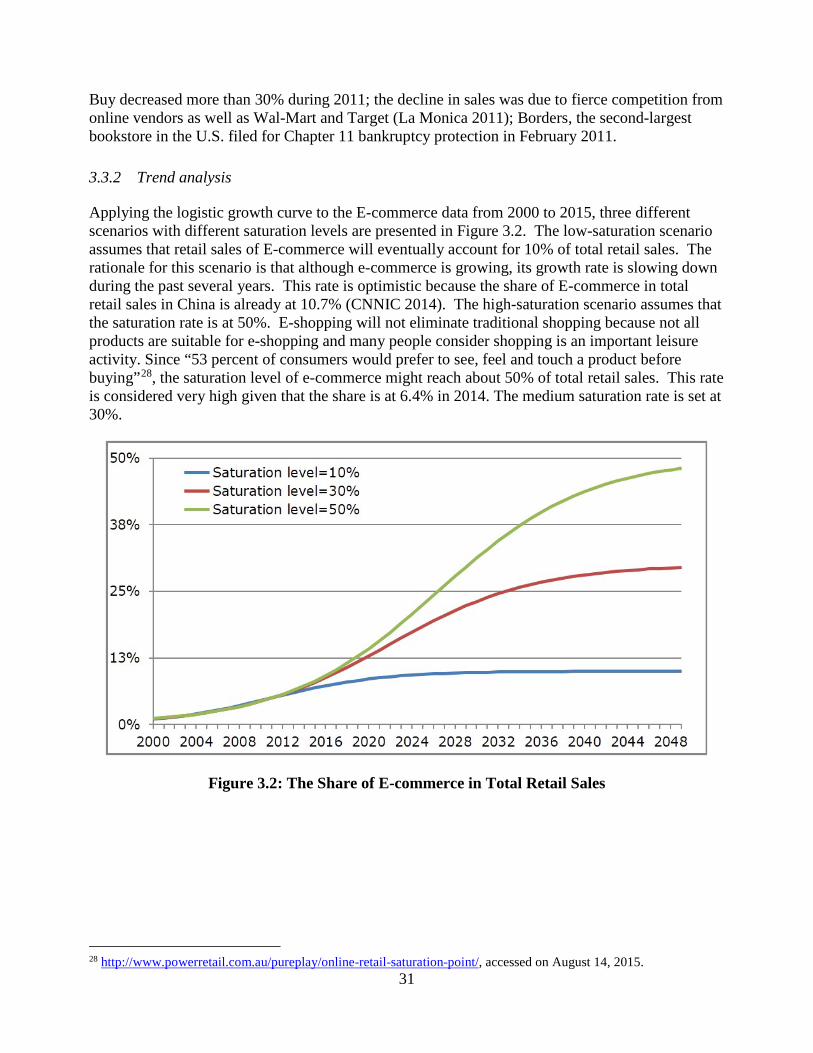
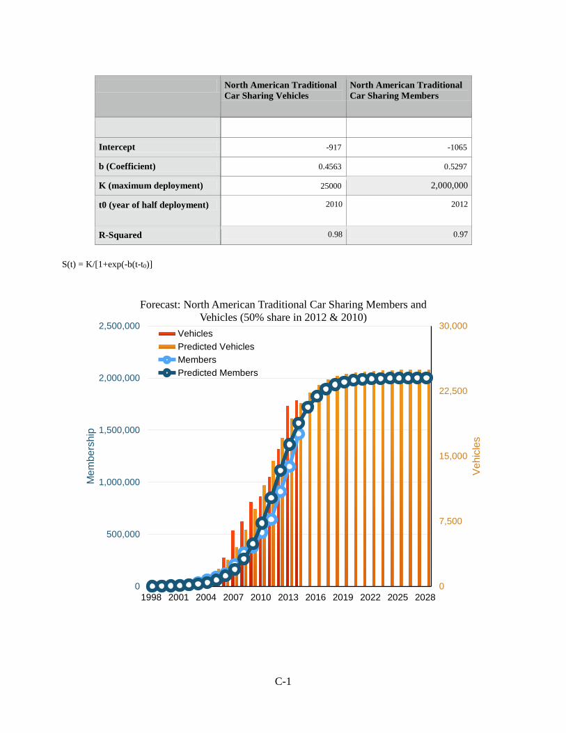
The ownership structure of automobiles will also change in coming years as Mobility-as-a-Service (MaaS) (Chapter 4) becomes more prominent. Sharing implies a reduction in auto ownership (increased mobility-as-a-service) in cities as car-sharing (Car2Go, Zipcar, Hourcar) and ride-sharing (Uber, Lyft, taxi) converge into a single driverless service that provides the right-size car for a given trip on a per-trip basis. While the degree to which people will give up the on-demand convenience of owning a car is unclear, it is far more likely in large cities where people rent apartments and car ownership is a hassle, than in rural areas, where response times of car rental will be larger. MaaS has a number of implications:

• The average age of the car will be younger, as shared vehicles are utilized more hours per day and turn-over more quickly. Cars become more like phones and less like long-lasting durable goods.

• The average size of car will be smaller as firms can right-size the fleet for demand, in contrast with privately owned cars, which are typically sized for extreme or unusual uses, rather than the daily one- or two-person trips.

• MaaS customers will travel less frequently than those who own cars, as they will pay out-of-pocket for capital costs each trip, while those who own cars forget about the sunk cost of ownership, which is paid for independent of the number of trips made.

• Streets will need to be redesigned to favor loading and unloading passengers, rather than on-street parking.

• Sharing implies an increased willingness to live in cities, which will be cleaner, safer, and more accessible with electric, automated, and shared vehicles respectively.

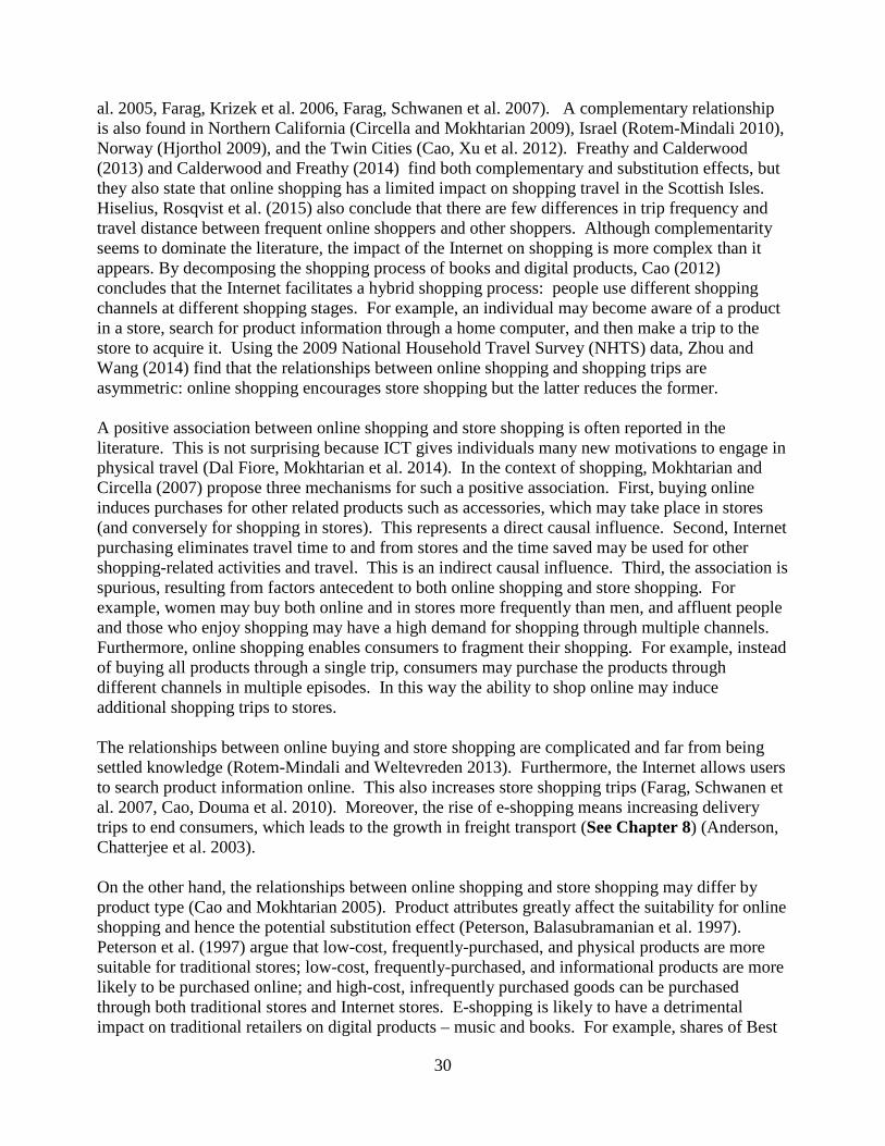
Information and communications technologies (Chapter 3) are changing travel demand patterns. Work at home, now at 4.4 percent, is rising, and while unlikely to replace all or even most work outside the home in the next two to three decades (when still fewer than 10 percent of workers are likely to work at home), it can certainly substitute in significant ways for many information economy jobs, and for the information-rich components of traditional jobs. Part-time telecommuting can reduce peak travel, both by shifting the time-of-day when commutes occur and avoiding it on select days altogether. Online shopping continues to grow, and is now about 8% of retail sales, and it could continue to rise to upward of 50% of retail activity, leading to a substitution of delivery for many more shopping tasks. The rise of virtual connectivity has occurred at the same time that the amount of in-person interaction has fallen in the past decade. Yet, information and communication technologies (ICT) not only reduce travel and but also induce new travel. For telecommuting, the key findings include the following:

• Telecommuting reduces commute travel during both peak and non-peak hours; • Telecommuting enables commuters to move farther away from their employment location

and become even more auto-dependent; • Telecommuting increases non-work travel, which takes place mostly close to home; • Telecommuting reduces vehicle miles traveled (VMT) slightly, but it helps mitigate the

growth of congestion on freeways; For e-shopping, the literature shows that

• Online searching is positively associated with store shopping and people who buy online also buy in person more;

• Studies are mixed on whether e-shopping reduces travel to stores and other leisure activities in the short term;

• E-shopping for now digital products (books, records, videos) has already changed retail patterns and shopping travel behavior;

• Online buying increases delivery traffic and freight transportation; • Existing studies are based on the small share of e-shopping in retail industries. If its share

is large enough to change the distribution of commercial land uses in the region, e-shopping will have a profound effect on shopping-related travel.

ICT are often promoted as a virtue alternative to physical travel, but transportation planners should be realistic about the relationships between ICT and travel: Although the short-term effect of ICT on travel may be substitution, in the long term, travel demand has historically grown as ICT demand increases. New sensors (Chapter 5) attached to the vehicle, person, and roadway will create increasing streams of information about real-time conditions on all transportation systems. This should have numerous applications, for instance, enabling transportation agencies to improve traffic signal

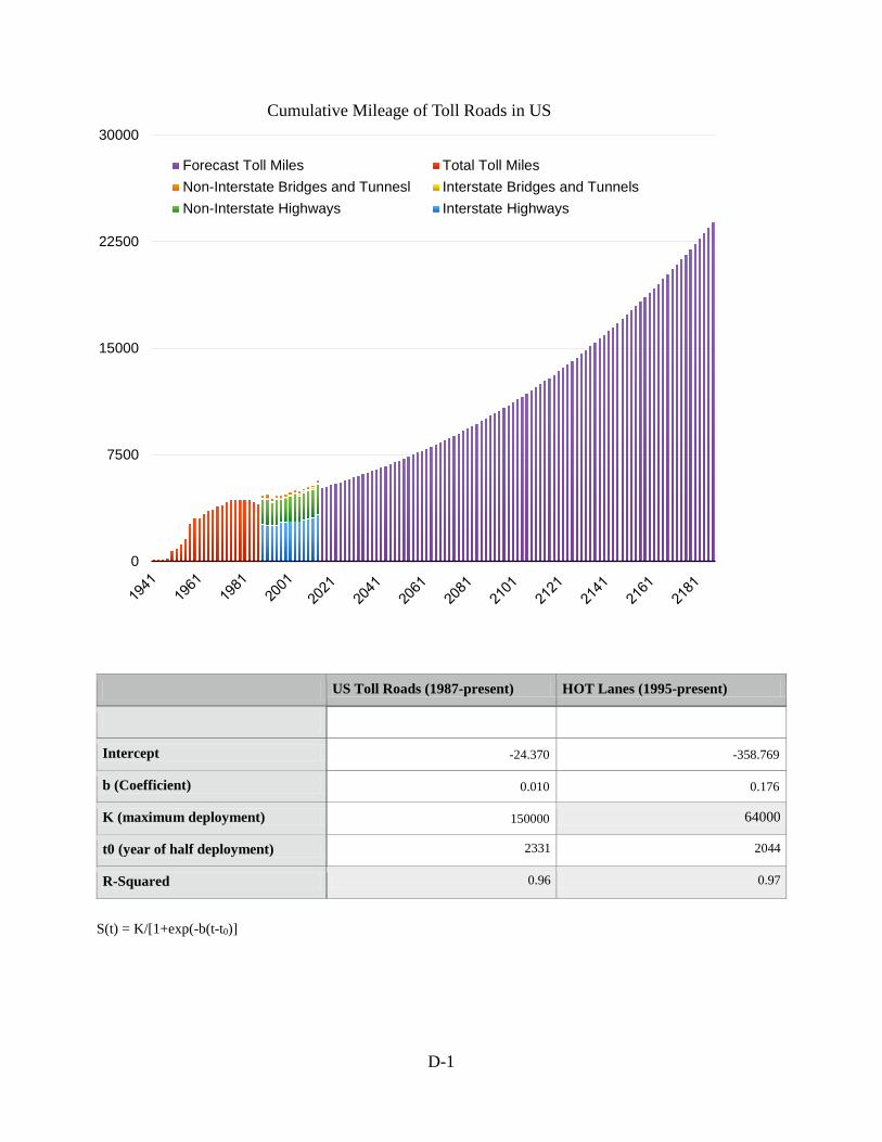
timing, and better matching of supply to demand. Connected vehicles are coming independent of automated vehicles. Whether the infrastructure providers add intelligence to their road and signal systems (for instance, telling vehicles when the light is about to change) is an open question. The potential transition away from gasoline is another important change confronting the transportation sector (Energy -Chapter 6). The timeline for electrification is similar but slower than that for automation. Though automated vehicles need not be electric, and electric vehicles need not be automated, we expect these systems to track and both see increasing deployment. If current trends hold, electric vehicles (EVs) may make up 68% of new car sales by 2050. This number is highly dependent on gasoline prices and environmental regulations. Minnesota will likely lag the US as the cold weather is less conducive to EVs than the US as a whole. Electricity generation costs are dropping, as are battery storage costs. There are new opportunities for in-roadway electric charging (dynamic wireless power transfer), probably beginning with buses at bus stops, that should be explored by transportation agencies. The advantage of such charging systems are a reduction in on-board battery storage weight required, which greatly improves vehicle efficiency (since energy is not consumed moving around stored energy). Gasoline remains the fuel to beat, and if gasoline costs remain low, electric vehicle deployment will be slower. Other fuels like methanol have an opportunity to become more significant, especially for truck fleets, for which electrification is much less efficient. Urban fleets with a lot of stop-start activity may see hybrid electric vehicles. We anticipate a reduction in energy consumption overall per distance traveled with reductions in vehicle weight for passenger cars and more efficient use of trucks (which are likely to get heavier, as they carry larger loads). Biofuel use for surface transportation is likely to plateau near existing use levels; however, it may increasingly be used in the electricity sector (and thus indirectly for an increasingly electrified transportation sector). Importantly, a reduction in gasoline consumption has large implications for transport financing. The lack of user fees for electric vehicles is a growing inequity that creates opportunities to move toward road pricing, as discussed below Pricing (Chapter 7) transportation proportionate to use has been a holy grail for transportation economists for decades. Pricing can be used to reduce or eliminate congestion by managing demand so that it does not exceed available supply. However, to date, it has been technologically and politically difficult to implement such a system. The advent of electronic toll collection (ETC) in the 1990s has resulted in a small resurgence in the number of toll roads, but there is no evidence that individual toll roads will expand to be a significant share of all roads anytime soon. Cities like Singapore, London, and Stockholm have established congestion charging zones. However, urban congestion charges have yet to be deployed in any large US city, and are unlikely to come to Minnesota before playing on the more congested New York, Los Angeles, San Francisco, and Chicago stages.

High occupancy toll lanes, such as the MnPASS lanes in Minnesota, are being deployed at a more rapid rate. The additional merit of these lanes is the opportunity to have this converted to serve automated-only traffic much sooner than all roads can be, providing a much higher throughput than general purpose lanes. This could occur as soon as 2025, and provide a decade of additional road capacity before human-driven cars are driven-off the freeway for the last time. Notably, EVs do not pay gas tax. (And hybrid electric vehicles pay much less per mile in gas tax than traditional internal combustion engine vehicles). As EVs gain market share, if the user-pays principle is to be maintained and reinforced, a new financing system needs to be found for these vehicles. This provides an opportunity to implement mileage charges with off-peak discounts, helping spread the peak and better-use road capacity. Phasing in road pricing one electric vehicle at a time seems the most promising strategy to deploy pricing on roads without the risks of a new large-scale system deployment. Logistics (Chapter 8) identifies a number of potential changes affecting the freight sector and how goods are delivered. Automation will affect deliveries as it has changed passenger transportation. A variety of automated delivery systems are likely to trialed in the coming decade, as distributors and retailers aim to connect directly to customers. On the logistics side, there are a number of changes enabled by information technologies. Supply chain network pooling and the physical Internet for long-distance shipments may become increasingly common as a means of getting better capacity utilization out of vehicles and drivers or vehicle controllers. Similarly efficiencies can be garnered through consolidated home delivery. All of these mean that fewer, but heavier trucks will be using Minnesota roads. Same day delivery in business-to-business, and more significantly, in business-to-consumer sectors is also likely to become more common, reducing shopping trips, and making online purchasing even more spontaneous, but in the net not affecting road usage much in terms of amount, but perhaps more in terms of additional traffic in evening and weekend periods. The overall conclusions are complex, but they suggest significant changes in the transportation sector over the coming few decades. Business-as-usual practices will need to change consistent with changing technologies and their effect on both supply and demand.

1

Chapter 1: Autonomous Vehicles

In March 2004, DARPA1 hosted the first Grand Challenge on vehicle automation. Set in the Mojave Desert (crossing the Nevada - California border), with $1 million going to the winner, the objective was for driverless cars to complete a 150 mile (240 km) route. Carnegie Mellon University's robot vehicle finished first, by completing almost 5 percent of the route, but was not awarded the prize. A second Grand Challenge was held in October 2005. Five vehicles completed the course, and Stanford

2University's team won with a time of just under 7 hours. In little over 18 months, vehicle automation technology rapidly improved. Two years later, in November 2007, DARPA established the Urban Challenge on a closed course at George Air Force Base. The 60 mile (96 km) route resembled an urban obstacle course. Carnegie Mellon took first, completing the run in just over 4 hours. Stanford secured second at just under four and a half hours. Unlike the Grand Challenges, cars had to have more sophisticated and intelligent sensors. Though road quality was better (paved rather than off-road), the challenge was far more challenging. A more important outcome (perhaps) is that Google hired many of the leaders of the Stanford and Carnegie Mellon teams,3 including Sebastian Thrun of Stanford and Chris Urmson of CMU, for their own internal secret project, which they announced in 2010. Google Cars had at that time driven 1,000 miles (1,600 km) without human intervention and 140,000 miles with limited control around the San Francisco Bay Area, see Figure 1.2.4 Google cars have now had more than a dozen crashes, and at least one of which resulted in injury. Google's official position is that none of the safety events were caused by Google’s vehicles or vehicle technology. There is some concern that automated vehicles have different driving styles than following human drivers may be used to, causing potential conflicts. To date, Google's cars are very map-dependent, running where the roads have been mapped out in detail, so that they can compare what they see with what they expect to see.5 That strategy has strengths and weaknesses. The strength is a reduction in computation costs and better understanding

1 DARPA stands for Defense Advanced Research Projects Agency; it is a unit of the Department of Defense, as

driverless cars have obvious military application. 2 Carnegie Mellon teams took second and third place. The Gray Insurance Company from New Orleans and Oshkosh

Trucks also completed the course. 3 Markoff, John (2010) Google Cars Drive Themselves, in Traffic. New York Times

http://www.nytimes.com/2010/10/10/science/10google.html?_r=2&src=sch&pagewanted=all Erico Guizzo (2011-10-18) How Google's Self-Driving Car Works IEEE Spectrum

http://spectrum.ieee.org/automaton/robotics/artificial-intelligence/how-google-self-driving-car-works 4 Source: Data on Google Cars from

140,000 - http://googleblog.blogspot.com/2010/10/what-were-driving-at.html 300,000 http://googleblog.blogspot.com/2012/08/the-self-driving-car-logs-more-miles-on.html 500,000 http://www.businessinsider.com/google-self-driving-car-problems-2013-3?op=1 700,000 http://googleblog.blogspot.co.uk/2014/04/the-latest-chapter-for-self-driving-car.html Nearly a million http://googleblog.blogspot.com/2015/05/self-driving-vehicle-prototypes-on-road.html

5 Alexis Madrigal @ The Atlantic: How Google Builds Its Maps—and What It Means for the Future of Everything – Technology : http://www.theatlantic.com/technology/print/2012/09/how-google-builds-its-maps-and-what-it-means-for-the-future-of-everything/261913/

2

and anticipation of the environment. Weaknesses include that (1) not everywhere is necessarily mapped, (there may be “Google deserts”, for instances some places are private property, and (2) the world changes, the map cannot be updated instantaneously. The first Google style AV to pass the unmapped or incorrectly mapped area will update the map as it passes, but it will of course need the capability of traveling with unmapped, incompletely mapped, or incorrectly mapped instances. And if it can do that autonomously, does it really need the map to proceed? It cannot do that autonomously, there remain issues with autonomous to human control interfaces.

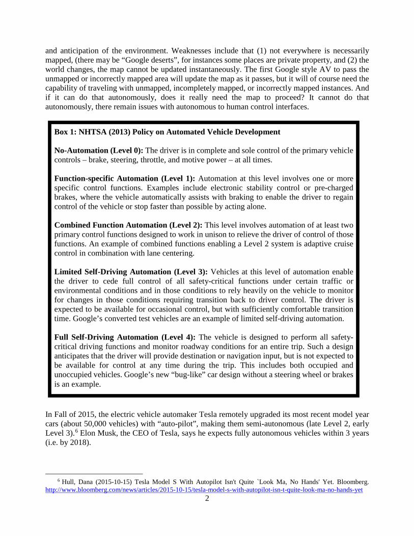
Box 1: NHTSA (2013) Policy on Automated Vehicle Development

No-Automation (Level 0): The driver is in complete and sole control of the primary vehicle controls – brake, steering, throttle, and motive power – at all times.

Function-specific Automation (Level 1): Automation at this level involves one or more specific control functions. Examples include electronic stability control or pre-charged brakes, where the vehicle automatically assists with braking to enable the driver to regain control of the vehicle or stop faster than possible by acting alone.

Combined Function Automation (Level 2): This level involves automation of at least two primary control functions designed to work in unison to relieve the driver of control of those functions. An example of combined functions enabling a Level 2 system is adaptive cruise control in combination with lane centering.

Limited Self-Driving Automation (Level 3): Vehicles at this level of automation enable the driver to cede full control of all safety-critical functions under certain traffic or environmental conditions and in those conditions to rely heavily on the vehicle to monitor for changes in those conditions requiring transition back to driver control. The driver is expected to be available for occasional control, but with sufficiently comfortable transition time. Google’s converted test vehicles are an example of limited self-driving automation.

Full Self-Driving Automation (Level 4): The vehicle is designed to perform all safety-critical driving functions and monitor roadway conditions for an entire trip. Such a design anticipates that the driver will provide destination or navigation input, but is not expected to be available for control at any time during the trip. This includes both occupied and unoccupied vehicles. Google’s new “bug-like” car design without a steering wheel or brakes is an example.

In Fall of 2015, the electric vehicle automaker Tesla remotely upgraded its most recent model year cars (about 50,000 vehicles) with “auto-pilot”, making them semi-autonomous (late Level 2, early Level 3).6 Elon Musk, the CEO of Tesla, says he expects fully autonomous vehicles within 3 years (i.e. by 2018).

6 Hull, Dana (2015-10-15) Tesla Model S With Autopilot Isn't Quite `Look Ma, No Hands' Yet. Bloomberg. http://www.bloomberg.com/news/articles/2015-10-15/tesla-model-s-with-autopilot-isn-t-quite-look-ma-no-hands-yet

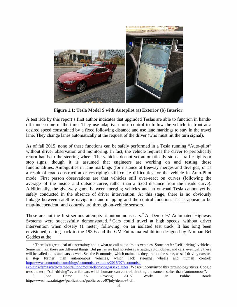
Figure 1.1: Tesla Model S with Autopilot (a) Exterior (b) Interior.

A test ride by this report’s first author indicates that upgraded Teslas are able to function in hands-off mode some of the time. They use adaptive cruise control to follow the vehicle in front at a desired speed constrained by a fixed following distance and use lane markings to stay in the travel lane. They change lanes automatically at the request of the driver (who must hit the turn signal).

As of fall 2015, none of these functions can be safely performed in a Tesla running “Auto-pilot” without driver observation and monitoring. In fact, the vehicle requires the driver to periodically return hands to the steering wheel. The vehicles do not yet automatically stop at traffic lights or stop signs, though it is assumed that engineers are working on and testing those functionalities. Ambiguities in lane markings (for instance at freeway merges and diverges, or as a result of road construction or restriping) still create difficulties for the vehicle in Auto-Pilot mode. First person observations are that vehicles still over-react on curves (following the average of the inside and outside curve, rather than a fixed distance from the inside curve). Additionally, the give-way game between merging vehicles and an on-road Tesla cannot yet be safely conducted in the absence of driver intervention. At this stage, there is no obviously linkage between satellite navigation and mapping and the control function. Teslas appear to be map-independent, and controls are through on-vehicle sensors.

These are not the first serious attempts at autonomous cars.7 At Demo '97 Automated Highway Systems were successfully demonstrated. 8 Cars could travel at high speeds, without driver intervention when closely (1 meter) following, on an isolated test track. It has long been envisioned, dating back to the 1930s and the GM Futurama exhibition designed by Norman Bel Geddes at the

7 There is a great deal of uncertainty about what to call autonomous vehicles. Some prefer “self-driving” vehicles. Some maintain these are different things. But just as we had horseless carriages, automobiles, and cars, eventually these will be called autos and cars as well. See the Economist, which maintains they are not the same, as self-driving cars are a step further than autonomous vehicles, which lack steering wheels and human control: http://www.economist.com/blogs/economist-explains/2015/07/economist-explains?fsrc=scn/tw/te/ee/st/autonomousselfdrivingcarsexplainer . We are unconvinced this terminology sticks. Google uses the term ”self-driving” even for cars which humans can control, thinking the name is softer than “autonomous”.

8 See Demo '97 Proving AHS Works in Public Roads http://www.fhwa.dot.gov/publications/publicroads/97july/demo97.cfm

3

4

1939 New York World’s Fair.

0

Cumulative miles traveled by Google Autonomous Vehicles

200,000

400,000

600,000

800,000

1,000,000

1,200,000

2010-10 2012-08 2013-03 2014-04 2015-05

Mile

s

Figure 1.2: Cumulative miles traveled by Google Autonomous Vehicles

While a technological success, the Automated Highway Systems programs were a political failure, and the program was cancelled. The reason for this is clear in retrospect: there was no deployment path. No one would build limited-access roads for a very few specialized cars. No one would buy cars that could be fully used only on selected lanes. Autonomous vehicles running in mixed traffic solve this chicken and egg problem, since they will be useful without special infrastructure, at the cost of much higher complexity. However, after a critical mass of autonomous vehicles hits the road, and once all the bugs are worked out, there will be potential gains (closer following, narrower lanes) for them to travel in autonomous-only lanes rather than mixed traffic. Existing managed lanes can be dedicated to AVs. Even general purpose lanes can be designated and redesigned to AV-only traffic in order to increase total system throughput. We may get special AV lanes on highways as an interim step before all lanes on all highways are for AVs only, and before non-AV cars are prohibited. New players like Google, Tesla, Uber, Apple and others are making serious investments in taking the driver out-of-the-loop for vehicle control. Further, after six decades of technological dormancy, the traditional automakers are responding to the DARPA Urban Challenge. For instance, Delphi, an auto parts manufacturer spun-off from General Motors, drove an automated Audi 3,500 miles (5,600 km) cross-country in March of 2015, with hands-off control 99 percent of the time.9 In fact, Delphi’s forerunner (GM Subsidiary) Delco sponsored a similar trip in 1995 by Carnegie Mellon scientists, where the computer navigated 98.7% of the time.10

9 Delphi completes first coast-to-coast automated drive http://www.kurzweilai.net/delphi-completes-first-coast-to-coast-automated-drive

10 Spice, Byron (2015-07-16) “Look, Ma, No Hands: CMU Vehicle Steered Itself Across The Country 20 Years Ago” https://www.cs.cmu.edu/news/look-ma-no-hands-cmu-vehicle-steered-itself-across-country-20-years-ago and Business Week (1995-08-13) “Look Ma, No Hands” http://www.bloomberg.com/bw/stories/1995-08-13/look-ma-no-hands

5

Advance still requires clarity about what 'automation' really means. As shown in Box 1, the National Highway Traffic Safety Administration (NHTSA) has a series of levels describing degree of autonomy (from Level 0 - "no autonomy" to Level 4 "full self-driving automation"). More early versions of autonomous cars are anticipated to be sold on the market for the 2017 Model Year (for instance Cadillacs with “SuperCruise”, which like Tesla vehicles with “Auto-pilot” may be described as somewhere between Level 2 "combined function automation" and Level 3 "limited self-driving automation"). Many of the necessary features like lane-keeping, adaptive cruise control, and automated braking technologies are already standard on high-end cars, as is automated parking assistance. None of the automakers advises hands-off driving at this point. Google itself 11 is aiming for Level 4, and believes that incremental changes like Level 3 are dangerous as once drivers cease paying attention it will be hard for them to reassert attention in a timely manner. In other words Google favors a large phase shift to AV for new vehicles. In contrast, traditional automakers are instead rolling out particular packages and features that still require the driver to attend to the driving task. The market and regulators will determine which of these two technological deployment paths actually occurs. The in-vehicle transition from autonomous mode to make the driver assume control is likely to be dangerous (though on the net, less dangerous than letting humans drive in the first place, otherwise the technology would not be permitted). 1.1 Connected vs. Autonomous Vehicles Some discussions conflate autonomous vehicle technology with "connected vehicle" technology. These are distinct, however, as the later allows individual vehicles to communicate with other nearby vehicles (vehicle to vehicle or V2V) and connected infrastructure (V2I) with Mobile Ad Hoc Networks. If widely deployed, this not only improves safety for those in the vehicle, it improves the safety and environment for pedestrians, bicyclists, and other drivers. Connected vehicles should enable vehicles to anticipate better and negotiate with each other for use of a particular bit of road space at a discrete point in time. Both autonomous and connected vehicles are coming. It is important to recognize that cars may be autonomous but not connected or connected but not autonomous, or both (or as today, neither). Connected vehicles and infrastructure in particular may be more vulnerable to hacking, though autonomous vehicles will likely have live connections to their manufacturer as well. The effects of autonomous vehicles are much more profound than connected vehicles, as connected vehicles are only especially useful in the presence of other connected vehicles, while autonomous vehicles are valuable through the transition period when most vehicles are not up-to-date.

11 Authors conversations with Google employees.

0

25

50

75

100

125

2015 2020 2025 2030 2035 2040

US New Car Market by NHTSA Automation Level (author estimates)

New Cars with Level 4New Cars with Level 3New Cars with Level 2New Cars with Level 1New Cars with Level 0

Figure 1.3: US New Car Market by NHTSA Automation Level (author estimates)

0

25

50

75

100

2015 2020 2025 2030 2035 2040

US Vehicle Fleet by NHTSA Automation Level

Fleet with Level 4Fleet with Level 3Fleet with Level 2Fleet with Level 1Fleet with Level 0

Figure 1.4: US Vehicle Fleet by NHTSA Automation Level

1.2 Timeline Cumulatively, the distances driven driverlessly are rising every year. This will take some time to perfect, but one day, in the near future, you may wake up, give a voice command to a car, and never again touch a steering wheel, gears, accelerator, or brakes (which won't be there)— as will everyone else. You will step into your car, tell it where to go, and not think about traffic. The window in front

6

7

of you will be a heads up display giving you information and entertainment, while allowing you to see the road coming up. To give a rough timeline, we anticipate Level 3 ("limited self-driving automation") autonomous vehicles will be on the market by 2020. We predict Level 4 will be available in 2025 and required in new US cars by 2030, and required for all cars by 2040. In other words, human drivers will eventually be prohibited on public roads. Consumer acceptance remains an unknown, and depends on the quality of the product being offered.

Automated vehicles are probably already legal in most US states (New York requires hands on the wheel),12 so the burden of proof is on those who want to slow them down. Several states, Nevada, Florida, California, Michigan, Virginia, and the District of Columbia, have passed special enabling legislation enabling testing of fully autonomous vehicles on public roads.

1.3 Environments The Cadillac SuperCruise entry into the "semi-autonomous" vehicle market implies the first market for autonomous vehicles would be the relatively controlled environment of the freeway.13 However, entry into the relatively controlled environment of low-speed places makes sense as well. These are two different types of vehicles (high speed freeway vs. low speed neighborhood), and though they may converge, there is no guarantee they will, and perhaps today's converged multi-purpose vehicle will instead diverge. There has long been discussion of Neighborhood Electric Vehicles, ranging from golf carts to something larger, which are in use in some communities, particularly southwestern US retirement complexes. In Sun City, Arizona, for instance, people use the golf cart not just for golfing, but for going to the clubhouse or local stores (usually as the household's second or third car, but occasionally as the primary vehicle). They can do this because local streets are controlled by low speed limits, and there are special paths where golf carts are permitted and other vehicles aren’t. Campuses, retirement communities, neighborhoods in some master planned communities, and true parkways are almost ideal for these types of “driverless carts”14 because these places don't have heavy traffic and discourage high speeds.

12 See Smith, B. W. (2012). Managing Autonomous Transportation Demand. Santa Clara Law Review, 52(4).

Weiner and Smith summarize the outstanding questions that legal regimes will need to better address to cope with driverless cars. Gabriel Weiner and Bryant Walker Smith, Automated Driving: Legislative and Regulatory Action, cyberlaw.stanford.edu/wiki/index.php/Automated_Driving:_Legislative_and_Regulatory_Action http://www.wired.com/2012/02/autonomous-vehicle-legality/

13 Nunez, Alex (2014-09-07) Cadillac will intro Super Cruise in 2017 flagship, V2V in CTS. Road and Track http://www.roadandtrack.com/new-cars/future-cars/news/a8626/cadillac-announces-super-cruise-and-v2v-tech-integration-for-2017-model-year/

14 We heard the term attributed to Bryant Walker Smith

8

1.4 Consequences Autonomous vehicles portend a series of consequences affecting both the transport sector and society, such as status. We highlight some below. Safety. Autonomous vehicles, powered by sensors, software, cartography, and computers can build a real-time model of the dynamic world around them and react appropriately. Unlike human drivers, they seldom get distracted or tired, have almost instantaneous perception-reaction times, and know exactly how hard to brake or when to swerve.

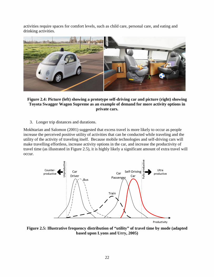
Cars would be much safer if only humans were not behind the wheel. It is possible to plausibly imagine a reduction from tens of thousands to hundreds of deaths per year in the US, upon full deployment. Vehicle Form. Autonomous vehicles promise a Cambrian explosion of new vehicle forms. Evidence for this is already emerging. Google has proposed and built prototypes of a new, light, low speed neighborhood vehicle designed for slow speed (25 mph or 40 km/h) on campuses. The UK has four pilot programs starting. Singapore is testing similar vehicles. This has important implications. For example, cars can be better designed for specific purposes, since, if they are rented on-demand or shared, they don't need to be everything to their owner. Narrow and specialized cars are more feasible in a world of autonomous vehicles. The fleet will have greater variety, with the right size vehicle assigned to a particular job. Today there is a car-size arms race, people buy larger cars, which are perceived to be safer for the occupant even if more hazardous for those around them, and taller cars, which allow the driver to see in front of the car immediately in front of them. Both of these advantages are largely obviated with autonomous vehicles. The car-size arms race ends. The low mass of neighborhood and single-passenger vehicles will save energy and reduce pavement wear, but also cause less damage when it (inadvertently) hits something or someone. Combining the low mass with the lower likelihood of a crash at low speed will magnify its safety advantage for non-occupants in this environment, compared with faster, heavier vehicles, which privilege the safety of the vehicle occupants. These savings will be passed on to consumers. Insurance companies will recognize the lower risks and lower rates. This will help drive adoption of autonomous vehicles. Alternatively, the auto-companies themselves may choose to accept liability for autonomous vehicles in autonomous mode, as some are already proposing. Capacity. Because they are safer, autonomous vehicles can follow other each other at a significantly reduced distance. Because they are safer and more precise and more predictable, autonomous vehicles can stay within

9

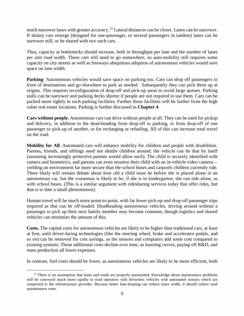
much narrower lanes with greater accuracy.15 Lateral distances can be closer. Lanes can be narrower. If skinny cars emerge (designed for one-passenger, or several passengers in tandem) lanes can be narrower still, or be shared with two such cars. Thus, capacity at bottlenecks should increase, both in throughput per lane and the number of lanes per unit road width. These cars still need to go somewhere, so auto-mobility still requires some capacity on city streets as well as freeways ubiquitous adoption of autonomous vehicles would save space on lane width. Parking: Autonomous vehicles would save space on parking too. Cars can drop off passengers in front of destinations and go elsewhere to park as needed. Subsequently they can pick them up at origins. This requires reconfiguration of drop-off and pick-up areas to avoid large queues. Parking stalls can be narrower and parking decks shorter if people are not required to use them. Cars can be packed more tightly in such parking facilities. Further those facilities will be farther from the high value real estate locations. Parking is further discussed in Chapter 4. Cars without people. Autonomous cars can drive without people at all. They can be used for pickup and delivery, in addition to the dead-heading from drop-off to parking, or from drop-off of one passenger to pick-up of another, or for recharging or refueling. All of this can increase total travel on the road. Mobility for All. Automated cars will enhance mobility for children and people with disabilities. Parents, friends, and siblings need not shuttle children around; the vehicle can do that by itself (assuming increasingly protective parents would allow such). The child is securely identified with camera and biometrics, and parents can even monitor their child with an in-vehicle video camera—yielding an environment far more secure than the school buses and carpools children currently ride. There likely will remain debate about how old a child must be before she is placed alone in an autonomous car, but the consensus is likely to be, if she is in kindergarten, she can ride alone, as with school buses. (This is a similar argument with ridesharing services today that offer rides, but that is to date a small phenomenon). Human travel will be much more point-to-point, with far fewer pick-up and drop-off passenger trips required as that can be off-loaded. Deadheading autonomous vehicles, driving around without a passenger to pick up their next family member may become common, though logistics and shared vehicles can minimize the amount of this. Costs. The capital costs for autonomous vehicles are likely to be higher than traditional cars, at least at first, until driver-facing technologies (like the steering wheel, brake and accelerator pedals, and so on) can be removed for cost savings, as the sensors and computers add some cost compared to existing systems. Those additional costs decline over time, as learning curves, paying off R&D, and mass production all lower expenses. In contrast, fuel costs should be lower, as autonomous vehicles are likely to be more efficient, both

15 There is an assumption that lanes and roads are properly maintained. Knowledge about maintenance problems

will be conveyed much more rapidly to road operators with driverless vehicles with automated sensors which are connected to the infrastructure provider. Because better lane-keeping can reduce lanes width, it should reduce total maintenance costs.

10

due to less congestion and more optimized driving styles ranging from smoother acceleration to various hypermiling techniques like drafting to reduce drag. Labor is a significant share of costs in transport, for vehicles such as taxis, buses, and trucks, which today require a driver. With automation that labor cost vanishes. We imagine a transitional phase where remote control drivers in a traffic center simultaneously monitor and manage multiple vehicles for situations when autonomous vehicles are not fully trusted. We expect those operators to be bored. This lower cost benefits taxis, buses, and trucks which had held higher labor costs relative to their competitors. There are additional labor costs associated with driving a private vehicle which don’t show up in the economic statistics, but can be quite expensive, particularly for high wage workers. This cost, too, will be reduced. Delivery services with online purchasing will become even more cost-competitive compared to traditional retail. Transit will either be more cost effective than it is now, or be able to offer lower fares, or some combination of the two. Right-of-Way Retrofit. To accommodate specialized low speed neighborhood or campus vehicles, most non-ideal places will require retrofits so that places can be connected with routes of low-speed. Retrofitting cities for transport has a long history as cities and transport technologies co-evolve. Cities, which had originally emerged with human and animal powered transport, were retrofitted first for streetcars, and then for the automobile, and in some larger cities for subways. We have also redesigned our taller buildings for escalators and elevators. Some places where retrofits might be required and feasible include cities laid out and built before the automobile. Much of the street grid can be retrofitted ("calmed") to disallow high-speed traffic, in much the same way bicycle boulevards are established. Similarly, retrofits are technically feasible anywhere there is space to install a slow network in parallel with the existing fast network, for instance, with barrier separated lanes on wider suburban roads. Vehicle diversity applies not only to a larger variety of motorized vehicles of various sizes, but also to a greater variety of transport using the existing streets, which today are highly segregated with cars (both moving and parked) dominating the street and pedestrians the sidewalk. Slow speed, light weight vehicles make shared spaces, which don't differentiate between the road and the sidewalk much more palatable. Roadspace Reallocation. It follows that if transport systems require reduced lane width and have adequate capacity, transport agencies can reduce paved area and still see higher throughput. Today, most roadspace is not used most of the time, but road agencies cannot just roll it up when it is not being used. However, on freeways the space can be deployed more dynamically to increase either safety (by increasing spacing) or capacity (by reducing spacing), simultaneously adjusting speed and spacing accordingly. Dynamically reversible lanes are possible once humans are out of the loop. On local streets, roadspace no longer required for motor vehicle movement can be reallocated to other uses (pedestrians, bicyclists, transit, parks and so on). But for purposes of reliability and safety, bikes, bus-rapid transit, and the newly emerging micro-transit modes benefit from priority lanes.

11

Nomadism. For a select few, driverless vehicles may bring back the recreational vehicle, as some choose the fully nomadic lifestyle, spending much if not most of their lives in motion, especially if energy costs are low. Driving style. A fundamental shift will occur once people no longer drive themselves. The preference that is felt for fast acceleration will diminish, permitting much more efficient engines (gasoline or otherwise). Ownership. Ownership of autonomous vehicles is a looming question. While most roads are public; most cars are private and individually owned. Most transit also is public, though services are sometimes performed under contract by private firms. Some private roads are emerging, but these roads are impossible without public approval and assistance. New technologies provide an opportunity to revisit old arrangements. New forms of ownership and payment will inevitably be a dynamic evolution. Customers would need to pay for services of any type (either as a subscription or a per-use basis). Advertising could offset—though not entirely cover—some costs. It is conceivable that stores might subsidize transport, as might employers, as benefits for the customers or staff (as they do today with parking). As discussed in the chapter on SHARING, Transport Network Companies such as Lyft and Uber compete with taxis. But with their added labor, such services are too expensive for most people for frequent mobility. Alternative ownership currently exists to some extent with the current carsharing companies (Car2go, Zipcar, etc.) which compete with rental cars. But again the cost is too high for most people to use on a daily basis for a primary mode of transportation, and unless they live in a place with many other users, the distance to the vehicle may be high. However, with autonomous vehicles, the cost of the driver can be skipped, the car can come to the traveler. In contrast, autonomous vehicles total costs will be significantly lower, making it feasible that larger numbers of people replace their personal car (which is parked 23 out of 24 hours) with one that comes on-demand. Status: Just as owning a car was once a class signifier in the US, and remains so elsewhere in the world, and as owning a particular model of car (like a Prius or a BMW) persists as a signifier, we can expect that during the transition period owning an autonomous car will be a class-signifier. It indicates at once that you are wealthy enough to own a new car, and technologically sophisticated enough to trust your life to it. While eventually we expect this to be uniform, early adopters will have very different economic and social characteristics from the population at large. During the long transition, those who cannot afford such cars may come to be vilified as the cause of crashes.

12

1.5 The Future of Travel Demand and Where We Live: The Out Scenario Autonomous vehicles will be faster. It will not escape the astute reader that, as the economists say “all else equal” faster vehicles increase demand. Will autonomous vehicles reverse the trends or plateauing or dropping per capita vehicle travel that we have seen for the past decade with existing technology? Will people make more trips? Will people make longer trips? Will people relocate? Each advance in mobility (the ability to go faster, either due to new technologies or more connected networks) has heretofore increased the size of metropolitan areas. People can reach more things in less time. Subways drove the expansion of London, while streetcars did the same for many American cities.16 Historically the time saved from mobility gains was used mostly in additional distance between home and workplace, maintaining a stable commuting (home to work) time. Recent evidence of average reduction in overall travel distances and time spent traveling presented is not as much about a reduction in trip distances between home and work (which if anything are still rising in the US) but a reduction in the number of work and other trips being made across the whole population. In short: speed decentralizes.17 Autonomous vehicles will likely be faster, particularly on freeways, especially after widespread deployment when all vehicles are autonomous. This will occur either once human cars are prohibited from freeways, or once a network of separate lanes are designated for autonomous cars. Coupling with just the faster speed, the fully autonomous vehicle lowers the cognitive burden on the former driver/now passenger. Modes with lower cognitive burden tend to have longer trip durations. Time is important, of course. What you can do with that time (the quality of the experience) also matters (See Chapter 2). If you can work while traveling, the value of saving time is less than if you must focus on the driving task. This may also explain the premium people are willing to pay for high-quality transit and intercity rail service.18 If the time or money cost of traveling per trip declines, the long-held theory of induced demand predicts, all else equal: more trips, longer trips, and peakier trips (more trips in the peak period). Privately owned autonomous vehicles lower the cost of travel per trip. Out: More vehicle travel with increased exurbanization. Fast, driverless cars that allow their passenger to do other things than steer and brake and find parking impose fewer requirements on the traveler than actively driving the same distance. Decreases in the cost of traveling (i.e., availability of multitasking) makes travel easier. Easier travel means increases in accessibility and subsequently increases in the spread of development and a greater separation between home and work, (pejoratively, sprawl), just as commuter trains today enable exurban living or living in a different

16 See Levinson, D. (2008). Density and dispersion: the co-development of land use and rail in London. Journal of

Economic Geography, 8(1), 55-77 and Xie, F., & Levinson, D. (2009). How streetcars shaped suburbanization: a Granger causality analysis of land use and transit in the Twin Cities. Journal of Economic Geography, lbp031.

17 In addition to speed anything that lowers the generalized cost of travel decentralizes. 18 Pursuit of high-specification ride-quality raises interesting issues about acceleration and motion sickness (which

is worse for passengers than drivers as passengers cannot anticipate as well as drivers). See Scott Le Vine, Alireza Zolfaghari and John Polak (2015), “Autonomous Cars: The Tension Between Occupant-Experience And Intersection Capacity,” Transportation Research Part C: Emerging Technologies

13

city.19 This reinforces the disconnected, dendritic suburban street grid and makes transit service that much more difficult (as if low density suburbs weren’t hard enough). People will live farther “Out”. It has been estimated that a 1 percent increase in accessibility leads to a 0.6 percent increase in travel.20 Couple this increase with the new mode of cars deadheading without people, and perhaps the doubling of capacities and speeds leads to a doubling of total travel, assuming nothing else changes. (Compare with the scenario presented in Chapter 4: Mobility-as-a-Service). Thus as the cost of travel decreases, people will be more willing to live in cities far from where they work. It is not uncommon for the Dutch to live on opposite sides of the country from where they work, relying on the train network. The Northeast Corridor of the US has people living in one city and commuting to another (for instance from Washington to Baltimore, Philadelphia to New York). At speeds of 100 miles per hour (160 km/h), the commuting range expands widely. It is entirely likely that such new e-propelled forms of transport, along with solar power, will greenwash a new generation of dispersed development, which may in fact net to a much smaller environmental footprint than today, if not a smaller footprint than future cities. The interplay of autonomous vehicles and pricing is especially important. While autonomous vehicle capacity eventually doubles or quadruples, per capita demand will rise as well if traditional patterns of induced demand hold, and people continue to work, shop, and play at today’s rates. It is quite possible that sharing (described in Chapter 4) remains a niche while most people choose to own their own cars — the “Out” scenario dominates. Thus exurbanization and cars driving around without people make extensive use of the newly available capacity. To fully mitigate these congestion effects, pricing is required.

1.6 Discussion Traffic congestion as a problem has the potential to diminish significantly if the capacity gains outweigh the increased demand they generate. People won't be driving themselves, but passenger-less cars will be moving all over the place. For personal travel, the question remains: rent or own? Will people with regular everyday trips find it cheaper to rent than own? The cost of ownership may turn out to be cheaper than the cost of rental in the cloud commuting model in many if not most US markets (outside central cities). Personally owned cars are not dead-heading everywhere for passengers, lowering energy and operational costs and wear and tear. Owners have more motivation to care for their own car (in subtle, non-detectable ways) than for a rental, so the car may last longer. Cloud commuting will permit much higher fleet turnover, and thus increase advanced technology penetration.

19 For more on this reasoning, see Chapter 11 in Levinson, D. and Krizek, K (2008) Planning for Place and Plexus: Metropolitan Land Use and Transport. Routledge.

20 Weis’ estimates give a demand elasticity of 0.6 to accessibility (Hansen style/log sum term) Weis, C. (2012) Activity oriented modelling of short- and long-term dynamics of travel behaviour, PhD Dissertation,

IVT, ETH Zürich, Zürich. Or a shorter version Weis, C. and K.W. Axhausen (2012) Assessing changes in travel behaviour induced by modified travel times: A

stated adaptation survey and modelling approach, disP, 48 (3) 40-53.

14

Continuing automation of vehicle technologies will lead to widespread deployment of driverless cars in mixed or eventually fully automated roadways. Eventually humans driving on public roads will be banned or greatly restricted. This has numerous implications. Chapter 4 considers the ownership model, and it is on ownership which turns the question of the travel demand and land use effects of Autonomous vehicles. Chapter 8 looks at issues of urban and long-haul freight transportation and automation, as well as local delivery. Other implications described in this chapter include those on for travel demand; safety; capacity; mobility for children, elderly, and disabled; transit; parking; and land use, population distribution and development. The authors anticipate that autonomous vehicles will go from their current status of 0% market share to an end state of 100% of all new car sales (i.e. autonomous capability will be a requirement of new car purchases). Further, older human-driven vehicles will be phased out except for special purposes (car shows, races, parades). A rough guide to the anticipated timeline is that NHTSA Level 4 cars (fully self-driving without human interaction) will enter the market between the 2020 and 2025 model years, and be required in all new cars by 2030, and by 2040 human-driven cars will be generally prohibited. Self-driving cars in specific contexts (e.g. freeways or isolated campuses) are expected enter the market before 2020. Current near-self-driving cars such as SuperCruise and the Tesla Model S are approximately NHTSA 2.5. While the end of state of autonomous vehicles presents a variety of benefits for travelers and transportation agencies alike, the adoption rate is unknown. It is far from clear the pace of change of autonomous vehicles. 1.7 Consequences

1. An increase in safety. This will reduce the number and severity of crashes. Follow-on

effects include a reduction in non-recurring congestion, and ultimately less resources spent on emergency response.

2. An increase in capacity as cars will be able to follow at closer headways. 3. An increase in capacity due to better lane-keeping. This will enable narrower lanes. 4. More opportunities for Mobility-as-a-Service [MAAS], and a potential change in

ownership structure. 5. A reduction in the effort (both physical and cognitive) associated with driving, which

should increase people’s willingness to travel for longer periods of time. 6. An increase in the speed of travel, which should increase people’s willingness to travel

longer distances. 7. An increase in mobility for those who now cannot drive (children, the disabled). This will

also increase the total amount of travel 8. A reduction in the space required for parking near the travelers destinations as cars can go

and park themselves. Further with Mobility-as-a-Service, cars may remain in use longer, and thus spend less time parked.

9. An increased ability to route vehicles in a system optimal way, as the computers doing routing can choose alternative algorithms.

10. Lowered labor costs for transit, trucks, and other service vehicles (e.g. snow plows). 11. Easier recharging for electric vehicles.

15

In the long run, this mostly suggests that less road capacity will be required per person. While longer trips, more trips, and increased mobility for the transportation disadvantaged (assuming vehicle ownership remains high, as opposed to a cloud commuting model) may offset some of the capacity gains, the capacity gains are likely to be large in the end. Other societal changes also generally point in that direction.

16

Chapter 2: Mobile Telecommunications and Activity In-Motion

2.1 Introduction The rise of mobile technologies have led to their increased use and increases in multitasking behavior while in-motion (enabled by technologies such as 4G, and in the future 5G and 6G phones and in-vehicle Wi-Fi). This research considers interactions including evidence from time use while traveling (reading, listening to music, work). Autonomous vehicles (see Chapter 1) will likely make this phenomenon more widespread. Better future telecommunication technology will also enable higher-bandwidth activities. Theory predicts that increasing use of telecommunications in motion makes travel time more useful, and this increases the willingness to travel. Note that telecommunications in general may enable less passenger travel with activities such as teleworking and e-shopping. This report focuses on telecommunications in motion and the impact of telecommunications on activities-in-motion. With more willingness to travel, people will presumably spend more time in motion. What types of activities can be carried out during travel in self-driving vehicles with better mobile technologies? How these activities differ from traditional activities that are conducted during travel on public transit vehicles? Will the self-driving and mobile technologies change spatial patterns of origins and destinations? Will trip chaining behavior become more popular? Will the behavior changes enabled by the self-driving and mobile technologies differ by gender, age, and socio-economic status (SES)? If so, how? And, what would be the societal impacts of these behavioral changes? These are the questions explored in this report. This chapter summarizes existing empirical evidence in the literature on activities in-motion. Then, the 2011-2014 American Time Use Survey data are used to explore new activities during travel, possibly enabled by self-driving and better mobile technologies. It then discusses how the technologies may influence car preferences, perceived utility of travel, spatial configurations of travel, including patterns of origins and destinations as well as trip chaining. How the effects may differ by personal socio-demographics and the societal implications of the effects are also discussed. 2.2 Existing Empirical Evidence Existing studies on mobile telecommunications and activity in-motion have focused on travel time use by rail and bus passengers. Recent research has shown that roughly 55% of rail passengers and 40% of bus passengers engage in technology, and that 30-40% of rail passengers work on board compared to roughly 10% report no use of travel time. Table 2.1 summarizes major time use activities reported as undertaken during travel in existing studies. Most studies listed in Table 2.1 are about time use during public transit trips. Only Malokin et al. (2015) and Mokhtarian et al. (2014) used samples of commuters including both transit commuters and commuters by other modes. Consequently, Malokin et al. (2015) included activities that are often considered as not suitable during transit trips, e.g., grooming and exercising.

17

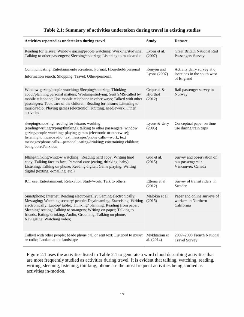
Table 2.1: Summary of activities undertaken during travel in existing studies

Activities reported as undertaken during travel Study Dataset

Reading for leisure; Window gazing/people watching; Working/studying; Talking to other passengers; Sleeping/snoozing; Listening to music/radio

Lyons et al. (2007)

Great Britain National Rail Passengers Survey

Communicating; Entertainment/recreation; Formal; Household/personal

Information search; Shopping; Travel; Other/personal. Kenyon and Lyons (2007)

Activity dairy survey at 6 locations in the south west of England

Window-gazing/people watching; Sleeping/snoozing; Thinking about/planning personal matters; Working/studying; Sent SMS/called by mobile telephone; Use mobile telephone in other ways; Talked with other passengers; Took care of the children; Reading for leisure; Listening to music/radio; Playing games (electronic); Knitting, needlework; Other activities

Gripsrud & Hjorthol (2012)

Rail passenger survey in Norway

sleeping/snoozing; reading for leisure; working (reading/writing/typing/thinking); talking to other passengers; window gazing/people watching; playing games (electronic or otherwise); listening to music/radio; text messages/phone calls—work; text messages/phone calls—personal; eating/drinking; entertaining children; being bored/anxious

Lyons & Urry (2005)

Conceptual paper on time use during train trips

Idling/thinking/window watching; Reading hard copy; Writing hard copy; Talking face to face; Personal care (eating, drinking, baby); Listening; Talking on phone; Reading digital; Game playing; Writing digital (texting, e-mailing, etc.)

Guo et al. (2015)

Survey and observation of bus passengers in Vancouver, Canada

ICT use; Entertainment; Relaxation Study/work; Talk to others Ettema et al. (2012)

Survey of transit riders in Sweden

Smartphone; Internet; Reading electronically; Gaming electronically; Messaging; Watching scenery/ people; Daydreaming; Exercising; Writing electronically; Laptop/ tablet; Thinking/ planning; Reading from paper; Sleeping/ resting; Talking to strangers; Writing on paper; Talking to friends; Eating/ drinking; Audio; Grooming; Talking on phone; Navigating; Watching video;

Malokin et al. (2015)

Paper and online surveys of workers in Northern California

Talked with other people; Made phone call or sent text; Listened to music or radio; Looked at the landscape

Mokhtarian et al. (2014)

2007–2008 French National Travel Survey

Figure 2.1 uses the activities listed in Table 2.1 to generate a word cloud describing activities that are most frequently studied as activities during travel. It is evident that talking, watching, reading, writing, sleeping, listening, thinking, phone are the most frequent activities being studied as activities in-motion.

18

Graph created by: Yingling Fan, U. of Minnesota

Data source: Activities mentioned in existing studies on travel time use.

THE USE OF TRAVEL TIME: MOST FREQUENTLY MENTIONED ACTIVITIES IN

Figure 2.1: Activities most frequency studied as activities during travel

Besides understanding how travel time is used, existing studies on the subjects have suggested the following: � Activities conducted during travel differ significantly by journey purpose and direction of

travel. Commuters are more likely to be engaged in work-related activities during work-related trips than leisure-related trips, and during morning commute trip than return-home trips.

� Activities differ significantly by gender, age, and class. Compared to men, women are more likely to spend travel time talking to other passengers and less likely to work or study. Older passengers are less likely to use smart devices during trips. Higher income commuters are more likely to use travel time to work and study.

� Activities differ by trip duration and items individuals have at hand. People are much more likely to do window gazing and people watching in trips of less than 15 min duration than in longer trips.

� Activities differ by environmental factors during the trip. Noise level significantly reduces the use of smart devices such as smartphones and iPads. Seating significantly increases the use of smart devices. Jerkiness reduces the likelihood of multitasking on bus.

Surveys on how air passengers value onboard Wi-Fi also provide insights into understanding the impact of telecommunications in motion. The 2014 Wireless Connectivity Survey includes more

19

than 1,000 adult flyers in the United States. The survey found that having access to onboard Wi-Fi not only affecting passengers’ flying experience, but also affecting passengers’ fight selections. In-flight Wi-Fi was found to influence flight selection for 66% of travelers, and 22% of the respondents said they have paid more for their ticket in order to fly on a Wi-Fi equipped aircraft. These survey results indicate that telecommunications in motion could have a significant impact on transportation mode choice, which is consistent with recent studies that suggest broadband access on public transportation systems increases ridership and encourages people to shift from cars to public transit modes (Frei and Mahmassani, 2011; Dong et al., 2015). Yet, it is important not to overstate the impacts of telecommunications on mode choice. Regardless of the age of the respondent, the two most important factors for choosing a public transit mode are total travel time (walking/cycling/driving + waiting + riding + walking/cycling/driving) and service reliability (Transit Center, 2014). As shown in Figure 2.2 below, access to Wi-Fi is a less important mode choice factor.

Figure 2.2: Potential Drivers of Transit Ridership by Age (Figure downloaded from Transit

Center, 2014)

2.3 Identification of New Activities in-Motion Using ATUS Data Analysis in this section uses publicly available data from the 2011-2014 American Time Use Survey (ATUS). ATUS involves computer-assisted telephone interviewing in which survey respondents are interviewed on the next day of a pre-selected day about how they spent their time from 4 AM on the pre-selected day to 4 AM of the interview day (days are selected to ensure

20

proportional distribution across the days of the week and even distyear) (Basner, et al., 2007). Each activity described by the respondscheme, going from a top-level category of activities, to subcategoactivities that describe very specific actions. To provide a specific “traveling” category includes a second-tier four-digit category of “and helping household members” under which “

ribution across the weeks of the ent is coded using a three-tiered ries, and then to third-tier example, the top-level two-digit traveling related to caring for

travel related to caring for and helping household children” is a third-tier activity with a six-digit activity code. ATUS data has a total of 465 six-digit activity codes, of which 6 indicate missing data status and 459 indicate activity information. Kenyon and Lyons’ (2007) had suggested that three attributes of activities may be important to the extent to which activity in-motion is both possible and desirable, including the degree of locational dependence, the degree of continuity of engagement, and the degree of active attention. Based upon their framework, the following two sets of activity attributes are important in identifying possible activities in-motion during the era of self-driving and better mobile technologies; � The degree of locational dependence (e.g., park use) and the necessity of importable

equipment (e.g., billiards) � The degree of engagement continuity and desired comfort level (e.g., uninterrupted

sleeping)

The degree of active attention will eventually be no longer important for enabling activity in-motion because, with fully self-driving cars, travelers are able to pay full attention to and be fully engaged in other activities. It is worth noting that, because most existing research have been about activities during bus/rail trips in public vehicles, the number of possible activities in-motion is likely to increase significantly after self-driving cars. Appendix A identifies possible activities that could be done in private vehicles. These activities have rarely being studied in the travel time use literature. They are: � A limited set of personal care activity including dressing & grooming, health-related self-

care, personal/private activities; � A limited set of child care activities including reading to/with children, home schooling,

and arts and crafts with children; � Eating and drinking; � Tobacco and drug use; and � Participation in religious practices.

Using the 2011-2014 ATUS data, Figure 2.3 presents the average daily time spent on the above activities by U.S. population aged 15 or older. On average, the U.S. population spent 118 minutes (roughly two hours) on these identified activity types. Note that child care and personal care activities included in Figure 2.3 are a limited set of these activities. Many child care and personal activities are location dependent and/or require importable equipment that cannot be conducted in travelling cars.

21

Child care Personal care

New activities becoming possible after self-driving cars (minutes)

0.36722.5532 3.155

46.0118

0.00

17.50

35.00

52.50

70.00

Eating and drinking Tobacco and druguse

Participation inreligious practices

66.6522

Figure 2.3: Average daily time spent on the identified new activities based upon 2011-2014

ATUS.

2.4 Impacts of the New Technologies

1. Unclear implications on mode choice.

Evidence has shown that use of information and telecommunication devices allows transit riders to stay connected, improves transit experience, potentially increase transit mode choice and ridership. Yet, there is also evidence that information and telecommunication technologies (ICTs) are the least important mode choice factor among people older than 30. Whether increasing available ICTs on public transit vehicles can shift people from driving to taking public transit is dependent upon the general performance of transit services such as service frequency, coverage, and reliability.

2. Bigger and smaller cars.

Most existing prototype self-driving cars appear to be small (see Figure 2.4 below). This is largely due to the early state of the technologies and the recognition that most travel is functional, for short distance trips, and involves one or two people. Further electric vehicles are presently constrained by batteries, and so there is a desire to limit vehicle weight to enable EVs. Once the technologies are mature, there could be large market demand for more space to increase activity options in the cars, particularly for longer distance (intercity) trips. As shown in Figure 2.3, most of the new

22

activities require spaces for comfort levels, such as child care, personal care, and eating and drinking activities.

Figure 2.4: Picture (left) showing a prototype self-driving car and picture (right) showing Toyota Swagger Wagon Supreme as an example of demand for more activity options in

private cars.

3. Longer trip distances and durations.

Mokhtarian and Salomon (2001) suggested that excess travel is more likely to occur as people increase the perceived positive utility of activities that can be conducted while traveling and the utility of the activity of traveling itself. Because mobile technologies and self-driving cars will make travelling effortless, increase activity options in the car, and increase the productivity of travel time (as illustrated in Figure 2.5), it is highly likely a significant amount of extra travel will occur.

Figure 2.5: Illustrative frequency distribution of “utility” of travel time by mode (adapted based upon Lyons and Urry, 2005)

23

4. Larger spatial footprints with more trip chaining behaviors

Mobile technologies offer more opportunities to replace hub-and-spoke trips toward a central point of gravity, with circular trips chained together (Dal Fiore et al, 2014). The saved travel time and the increased utility of travel are likely to encourage visits to more distant but more attractive destinations (Dal Fiore et al, 2014).

Figure 2.6: A two-step hypothesis on the implications of mobile technology for spatial

behavior. Step 1: circular trips replace hub-and-spoke trips to and from a point of gravity; Step 2: the number of trips increases (and/or chosen destinations for existing trips change)

due to increased efficiency and information. (Figure downloaded from Dal Fiore et al, 2014)

5. Behavioral impacts of technologies are likely to differ by gender, age, and SES.

Complex interaction effects are likely to occur when it comes to how the technologies may affect trip distance, duration, activity space, trip chaining, and car preferences across population groups. For example, women have traditionally commuted shorter distances but travel more for household support than men, which had led to limited economic opportunities for women. Self-driving cars may enable women travel farther for jobs because an increased number of personal care and child care activities can be done in self-driving cars. Mobile technology and self-driving cars may also enable women to travel less for errands because more errands can be done online and self-driving cars encourage trip chaining activity.

6. Societal implications

Mobile technology and self-driving cars are likely to have fundamental societal impacts such as transforming urban form and improving transportation equity. For example, although technologies may encourage extra travel for people with resources, they could also eliminate the needs for travel and the needs for auto ownership among people with lower incomes (see Chapter 4). Contingent on continued private vehicle ownership, people will be more likely to make housing location choices based on their residential preferences (such as school quality, neighborhood security, neighborhood cohesion etc.) than based upon spatial accessibility. As people who own autonomous vehicles are more willing to travel farther for more attractive destinations, fewer but larger business centers are expected.

24

Chapter 3: Information and Communication Technologies

3.1 Introduction It is well perceived that information and communication technologies (ICT) have had pervasive impacts on modern society - they are changing how and where we work, shop, and in other ways live our lives. ICT, particularly the Internet and mobile service, make virtual activities a viable alternative to traditional physical activities. The growing penetration of ICT has important implications on transportation system. Unsurprisingly, transportation policy-makers and planners expect tele-activities to replace some activities that require travel between places and hence alleviate transportation and related problems that many large metropolitan areas are confronting. However, research conducted during past decades indicates that the impact of ICT on activity participation and travel is more complex than it appears at first glance. This report summarizes the effect of telecommuting and teleshopping on individuals’ travel behavior based on the literature, and discusses their potential impact on transportation system by 2040. It then summarizes the effects of other tele-activities on travel. The final section offers an overall summary and reviews reasons why ICT are unable, by themselves, to solve transportation problems, but do bring about new challenges to our transportation systems. 3.2 Telecommuting Telecommuting has grown considerably during the past few decades. Employees who primarily work at home increased by 61% from 2005 to 2009 and in 2010 about 16 million employees worked at home at least once a month, an increase of 62% from 2005 (Lister and Harnish 2011). Telecommuting has particular appeal because of its potential to reduce commute travel and traffic congestion during peak hours, and energy consumption, and air pollution. 3.2.1 The impacts of telecommuting on transportation Conceptual and empirical studies in the field of ICT and transportation suggest that telecommuting may interact with travel behavior in four ways: substitution, complementarity, modification, and neutrality (Salomon 1986, Mokhtarian 1990). Substitution denotes that an individual works at home instead of making a physical trip to her workplace. Complementarity means that telecommuting generates new demands for other non-work trips. Modification denotes that telecommuting does not affect the total amount of commute travel but changes the characteristics of trips such as mode choice, timing, and chaining. Neutrality means that telecommuting has no impacts on travel behavior. Among the four ways, transportation planners are most interested in substitution. The relationships between telecommuting and travel behavior vary based on the measures of travel behavior. For example, an individual replaces a commute trip by working at home, but she makes a nonwork trip because of time savings from not making the commute trip. In this case, the former represents a substitution effect and the latter is a complementary effect. The net effect of telecommuting on total travel depends on the characteristics of the commute and nonwork trips. If the nonwork trip is longer than the commute trip, the net effect is complementarity. If the nonwork trip is shorter than the commute trip, the net effect is substitution. If the two trips have the same

25

length but take place at different times (such as peak vs. non-peak hours), the net effect can be classified as modification. Significant research has been conducted to understand the impact of ICT on where work is done and how this affects travel. Not surprisingly, previous studies offer mixed results. Pendyala et al. (1991) found that telecommuters not only reduced commute trips, but also chose non-work destinations close to their home. By contrast, Gould and Golob (1997) found that telecommuters generated new non-work trips, which offset the benefits of saved commute trips. Using the 1991 Caltrans Statewide Travel Survey, Mokhtarian and Henderson (1998) found that home-based workers and non-home-based workers made a similar number of trips: the savings from commute trips of home-based workers are almost completely offset by the increase in their non-work trips. Several studies have found that telecommuting is positively associated with commute distance (Mokhtarian, Handy et al. 1995, Zhu 2012). Because researchers are unsure about which comes first, telecommuting or residential location, the association may result from two potential causes: One mechanism is that individuals choose to telecommute because they want to reduce the cost associated with their long commute distance; and the rival mechanism is that individuals choose to live farther away from their workplaces because they are able to telecommute (Ory and Mokhtarian 2006). If the latter prevails, telecommuting may have an adverse effect on VMT. For example, telecommuters may choose to live in far-flung exurban or rural areas where they depend more on private vehicles for their daily life than living in urban areas. Using the 2001 and 2009 National Household Travel Survey (NHTS), Zhu (2012) explored the impacts of telecommuting on travel behavior. He used the use of the Internet as an instrument to predict the probability of telecommuting, and then used the predicted probability of telecommuting to explain travel behavior. He found that telecommuting has positive associations with the following behavioral variables: one-way commute distance, one-way commute duration, total work-trip distance, total work-trip duration, total work-trip frequency, total non-work-trip distance, total non-work-trip duration, and total non-work-trip frequency. Overall, he concluded that telecommuting did not reduce but increase travel. By contrast, an aggregate time series analysis showed that telecommuting reduced vehicle miles travelled (VMT) by about 0.8% or less (Choo, Mokhtarian et al. 2005). After reviewing more than 30 empirical studies, Andreev et al. (2010) concluded that telecommuting tends to reduce various measures of travel in the short run, but its long-term impact is uncertain, partly because of induced travel demand and residential location choice impacted by the ability of telecommuting. 3.2.2 Trend analysis In the American Community Survey (ACS), respondents were asked to indicate “what was your primary means of transportation to work during the survey week?” The choice set includes: � Car, truck, or van - driving alone � Car, truck, or van - carpooled � Public transportation � Walked � Taxi, motorcycle, or bike

26

� Worked at home Work at home (WAH) is the third commonly chosen primary means of transportation, after driving alone and carpooling. In 2013, the share of workers who worked at home was about 25% more than that of workers who took public transportation21. Note that this underestimates the share of less used modes, for instance, for people who work-at-home twice a week and drive three times will be reported as driving by 100% of those respondents. Applying the logistic growth curve to the ACS WAH data from 2005 to 2013, three different scenarios with different saturation levels are presented in Figure 3.1. The low-saturation scenario assumes that WAH workers will eventually account for 10% of the total workforce in the US. The rationale for this scenario is that although WAH is generally growing, its growth is slow, on average at about 2.5% annually during the past decade. The share of WAH workers was at 4.4% in 2013 and it will take more than three decades to reach the saturation level if the growth rate remains stable. The high-saturation scenario assumes that the maximum level is at 40%. This is consistent with Handy and Mokhtarian (1996). Their assumption was drawn from Nilles’s assumption that “information workers” account for about 50% of the work force, and 80% of information workers have the potential to telecommute (Nilles 1988). Using California data, Handy and Mokhtarian also showed that the assumption is consistent with “the characteristics of the California work force and with studies of telecommuters” (p. 171). This saturation rate is also consistent with the estimates of Global Workplace Analytics22: 50% of jobs are compatible with telework and 79% of workers want to telecommute (50%*79%=40%). The medium saturation rate is set at 20%. As shown in Figure 3.1, the share of WAH workers will grow to 6.7% ~ 7.6% under the three scenarios by 2040. This represents an increase of 2.3 ~ 3.2 percentage points over the 2013 level. The growth is not substantial, but it is also non-trivial because the impact of travel reduction on congestion level is exponential.

21 http://www.newgeography.com/content/004933-working-home-in-most-places-big-alternative-cars, accessed on August 14, 2015 22 http://globalworkplaceanalytics.com/telecommuting-statistics, accessed on August 14, 2015.

27

0%

2%

5%

7%

9%

2001 2005 2009 2013 2017 2021 2025 2029 2033 2037

Saturation level=10%Saturation level=20%Saturation level=40%

Figure 3.1: The Share of Work-at-Home Workers in Workforce

It is worth noting that WAH workers in the Census or ACS include self-employed workers such as farm, domestic, and service workers. Their home-based work does not substitute for a commute so they are not telecommuters per se (Mokhtarian, Salomon et al. 2005). Therefore, we are likely to misestimate the number of telecommuters. In 2005, 3.62% of the work force worked at home. Excluding the self-employed workers, about 1.37% of workers considered their home primary workplace. That is, self-employed workers accounted for about 2.24%. In 2012, employee teleworkers totaled about 3.3 million23, accounting for 2.3% of the work force, whereas self-employed workers accounted for 2.03%. Further, the ACS does not consider occasional telecommuters, who do not choose home as their primary workplace. That is, the ACS undercounts the number of telecommuters. However, because there is no consensus on how to define telecommuting, reliable historical data on the number of telecommuters in the USA are not available (Mokhtarian, Salomon et al. 2005). WorldatWork Survey estimated that about 16 million workers telecommuted at least once a month in 2010 (Lister and Harnish 2011). This accounted for about 11% of the work force. This number is expected to grow. However, in terms of telecommuting frequency, the followers tend to telecommute less often than early adopters of telecommuting (Handy and Mokhtarian 1996). However, telecommuting frequency should be smaller than this rate because working at home includes work after regular hours and employees may work at home partly while working at regular workplace.

23 http://globalworkplaceanalytics.com/telecommuting-statistics, accessed on August 14, 2015.

The ACS does not capture those who work at other places such as client offices, telecenters, coffee shops, and vehicles (Lister and Harnish 2011). In the 1990s, neighborhood telecenters were promoted in California, under the sponsorship of the State of California Department of Transportation (Caltrans) with funding from the Federal Highway Administration (Varma, Ho et al. 1998). However, the pilot program was not promising and hence discontinued. There are also 53 million freelancers in the USA, who account for 34% of the work force24. Some of them work in coffee shops or libraries although the exact number is unknown. Many freelance as a second or third job. An employees’ decision to telecommute and hence the penetration of telecommuting is affected by employers’ attitudes toward teleworking. Although telecommuting has the potential to increase productivity and save office-related costs, managers worry about the lack of team-building, commitment, and control (Baruch 2000). In 2013, Hewlett-Packard required most of their employees to work at the office instead of from home in the name of building engagement, collaboration and innovation25. Yahoo and Best Buy also implemented similar polices to scale down or abandon their telecommuting programs26. 3.2.3 Perspective Based on the American Community Survey, an additional 3% of the work force may work at home by 2040. Although the literature offers mixed evidence on the impact of telecommuting on travel, it is expected to help reduce commute travel during peak hours. However, the ability to telecommute may motivate workers to relocate farther away from workplace in the long term. This will increase commute distance on non-telecommuting days and may result in increases in distance traveled by automobile. Travel time savings from telecommuting will bring about additional non-work travel, which offsets the benefits of telecommuting. Since non-work travel tends to occur closer to home than commute trips, telecommuting is expected to reduce VMT slightly (Choo, Mokhtarian et al. 2005). Because telecommuters’ activity space is closer to home than to work on telecommuting days (Saxena and Mokhtarian 1997), telecommuting will help ease traffic congestion on the freeways and around employment centers even if the number of trips (including both commute and non-work travel) is the same on telecommuting and non-telecommuting days. Although coffee shops have become a new workplace for many workers, they are not expected to materially influence vehicular travel, similar to neighborhood telecenters. In particular, workers at neighborhood telecenters tend to have a higher number of return home trips and other non-work trips on telecommuting days and they also tend to shift from other modes to driving alone (Balepur, Varma et al. 1998). The potential increases in engine cold starts will further reduce the environmental benefits of telecommuting. It is worth noting that ICT have made traditional “9-5” work schedule and fixed locations obsolete. People can work at home, at restaurants, while travelling and at any time when it is convenient. 24 https://www.freelancersunion.org/blog/dispatches/2014/09/04/53million/, accessed on August 14, 2015. 25 https://www.flexjobs.com/blog/post/hewlett-packard-bans-telecommuting-quite/, accessed on September 30, 2015. 26 http://www.theguardian.com/sustainable-business/working-from-home-yahoo-best-buy-hp-moves, accessed on September 30, 2015.

28

29

People can work remotely as well as at primary office in a day. Therefore, not all the implications of teleworking relate to transportation. 3.3 E-shopping “Shopping online is about to explode. Retailers of all types are expanding product offerings, adding in-store pickup, free shipping and experimenting with social media. It’s getting harder to tell pure play Internet retailers from the bricks and mortar shops with online portals, and all of them are reinventing how we’ll shop online in the future” (Heller 2011). In 2000, retail sales of E-commerce27 in the USA totaled about $27.5 billion, according to US Census E-commerce Report. In 2014, the sales have increased to $297.5 billion. The 10-fold growth of E-commerce signifies its pervasive impacts on retail industries as well as transportation. 3.3.1 The impacts of e-shopping on transportation Transportation planners are interested in the changes that e-shopping will bring to transportation system. In particular, planners tend to focus on the effects of e-shopping on individuals’ activity-travel patterns. The potential of online buying to substitute for traditional in-store shopping and reduce personal shopping travel has important implications for travel demand management and congestion mitigation. According to the 2001 National Household Transportation Survey (NHTS), on average shopping travel accounted for 14.4% of annual VMT per household and 21.1% of annual vehicle trips per household (Hu and Reuscher 2004). Therefore, the growth of online buying could have the potential to reduce traffic if it does replace physical shopping – substitution. On the other hand, if e-shopping induces new shopping trips, it is likely to generate more personal travel to existing transportation systems – complementarity. What does the literature say on the impact of e-shopping on traditional store shopping? Some descriptive studies offer mixed outcomes. Cairns et al. (2004) report that online shopping reduces at least one vehicular trip for 80% of 538 U.K. Internet users polled by British Telecom. However, Sim and Koi (2002) state that 88% of 175 Singapore online buyers do not observe any influence on their travel to stores. Corpuz and Peachman (2003) show that 14% of respondents in Sydney would have not made the purchase if online shopping were not available and 19% would have made a special trip to stores. That is, online shopping not only induces consumption but also replaces physical trips. Several multivariate analyses have been conducted to understand the relationships between online shopping and store shopping. Using the 2000 San Francisco Bay Area Travel Survey, Ferrell (2004, Ferrell 2005) employs two-step linear regression and structural equation models, respectively, to examine the impacts of teleshopping on shopping-related travel behavior. In the two studies, he finds substitution, complementarity, and neutrality depending on the dependent variables of interest. Farag and colleagues conducted a series of studies in the Netherlands and find that online shopping frequency is positively associated with store shopping frequency, even after controlling for shopping attitudes and/or demographics such as income (Farag, Schwanen et

27 US Census E-commerce Report defines E-commerce sales as “sales of goods and services where the buyer places an order, or the price and terms of the sale are negotiated, over an Internet, mobile device (M-commerce), extranet, Electronic Data Interchange (EDI) network, electronic mail, or other comparable online system” although offline payments are possible. https://www.census.gov/retail/index.html#ecommerce, accessed on August 14, 2015.

30

al. 2005, Farag, Krizek et al. 2006, Farag, Schwanen et al. 2007). A complementary relationship is also found in Northern California (Circella and Mokhtarian 2009), Israel (Rotem-Mindali 2010), Norway (Hjorthol 2009), and the Twin Cities (Cao, Xu et al. 2012). Freathy and Calderwood (2013) and Calderwood and Freathy (2014) find both complementary and substitution effects, but they also state that online shopping has a limited impact on shopping travel in the Scottish Isles. Hiselius, Rosqvist et al. (2015) also conclude that there are few differences in trip frequency and travel distance between frequent online shoppers and other shoppers. Although complementarity seems to dominate the literature, the impact of the Internet on shopping is more complex than it appears. By decomposing the shopping process of books and digital products, Cao (2012) concludes that the Internet facilitates a hybrid shopping process: people use different shopping channels at different shopping stages. For example, an individual may become aware of a product in a store, search for product information through a home computer, and then make a trip to the store to acquire it. Using the 2009 National Household Travel Survey (NHTS) data, Zhou and Wang (2014) find that the relationships between online shopping and shopping trips are asymmetric: online shopping encourages store shopping but the latter reduces the former. A positive association between online shopping and store shopping is often reported in the literature. This is not surprising because ICT gives individuals many new motivations to engage in physical travel (Dal Fiore, Mokhtarian et al. 2014). In the context of shopping, Mokhtarian and Circella (2007) propose three mechanisms for such a positive association. First, buying online induces purchases for other related products such as accessories, which may take place in stores (and conversely for shopping in stores). This represents a direct causal influence. Second, Internet purchasing eliminates travel time to and from stores and the time saved may be used for other shopping-related activities and travel. This is an indirect causal influence. Third, the association is spurious, resulting from factors antecedent to both online shopping and store shopping. For example, women may buy both online and in stores more frequently than men, and affluent people and those who enjoy shopping may have a high demand for shopping through multiple channels. Furthermore, online shopping enables consumers to fragment their shopping. For example, instead of buying all products through a single trip, consumers may purchase the products through different channels in multiple episodes. In this way the ability to shop online may induce additional shopping trips to stores. The relationships between online buying and store shopping are complicated and far from being settled knowledge (Rotem-Mindali and Weltevreden 2013). Furthermore, the Internet allows users to search product information online. This also increases store shopping trips (Farag, Schwanen et al. 2007, Cao, Douma et al. 2010). Moreover, the rise of e-shopping means increasing delivery trips to end consumers, which leads to the growth in freight transport (See Chapter 8) (Anderson, Chatterjee et al. 2003). On the other hand, the relationships between online shopping and store shopping may differ by product type (Cao and Mokhtarian 2005). Product attributes greatly affect the suitability for online shopping and hence the potential substitution effect (Peterson, Balasubramanian et al. 1997). Peterson et al. (1997) argue that low-cost, frequently-purchased, and physical products are more suitable for traditional stores; low-cost, frequently-purchased, and informational products are more likely to be purchased online; and high-cost, infrequently purchased goods can be purchased through both traditional stores and Internet stores. E-shopping is likely to have a detrimental impact on traditional retailers on digital products – music and books. For example, shares of Best

31

Buy decreased more than 30% during 2011; the decline in sales was due to fierce competition from online vendors as well as Wal-Mart and Target (La Monica 2011); Borders, the second-largest bookstore in the U.S. filed for Chapter 11 bankruptcy protection in February 2011.

3.3.2 Trend analysis Applying the logistic growth curve to the E-commerce data from 2000 to 2015, three different scenarios with different saturation levels are presented in Figure 3.2. The low-saturation scenario assumes that retail sales of E-commerce will eventually account for 10% of total retail sales. The rationale for this scenario is that although e-commerce is growing, its growth rate is slowing down during the past several years. This rate is optimistic because the share of E-commerce in total retail sales in China is already at 10.7% (CNNIC 2014). The high-saturation scenario assumes that the saturation rate is at 50%. E-shopping will not eliminate traditional shopping because not all products are suitable for e-shopping and many people consider shopping is an important leisure activity. Since “53 percent of consumers would prefer to see, feel and touch a product before buying”28, the saturation level of e-commerce might reach about 50% of total retail sales. This rate is considered very high given that the share is at 6.4% in 2014. The medium saturation rate is set at 30%.

0%

13%

25%

38%

50%

2000 2004 2008 2012 2016 2020 2024 2028 2032 2036 2040 2044 2048

Saturation level=10%Saturation level=30%Saturation level=50%

Figure 3.2: The Share of E-commerce in Total Retail Sales

28 http://www.powerretail.com.au/pureplay/online-retail-saturation-point/, accessed on August 14, 2015.

32

In the low-saturation scenario, the share of e-shopping will reach 90% of the saturation level (9%) in 2023. In the medium-saturation scenario, the share of e-shopping will reach 90% of the saturation level (27%) in 2037. In the high-saturation scenario, the share of e-shopping will reach 90% of the saturation level (45%) in 2042. This implies that the peak impact of e-shopping on traditional shopping is likely to occur within the time frame of the next long-range transportation plan. 3.3.3 Perspectives Though shopping travel has declined over the past decade (as discussed above and in Chapter 8), there is to date no persuasive causal evidence that online shopping is responsible, and the degree to which it has the potential to significantly reduce individuals’ shopping trips to stores in the future remains uncertain. Most studies concluded a complementarity effect of e-shopping on traditional store shopping (Andreev, Salomon et al. 2010). Although a few activity-based studies found that e-shopping tends to reduce shopping travel and other leisure activities (Ferrell 2004, Ferrell 2005, Ding and Lu 2015), activity diaries conducted for one day are not long enough to capture the whole process of e-shopping, which can take days or even weeks to complete because of its temporal fragmentation. Because almost all existing studies are based on relatively low shares (less than 10%) of e-commerce in total retail sales, it is less certain about the relationships between e-shopping and store shopping when the share grows much higher. However, since ICT tends to have a dominant complementary effect on transportation in the long run (Choo, Lee et al. 2007), it is not unreasonable to expect that the number of shopping trips will grow or at least stay the same, whereas the delivery trips and freight transport associated with e-shopping will definitely grow. If the saturation rate of e-commerce is at 30% or higher, the delivery traffic on local streets will increase substantially. The bypass of wholesalers and retailers in the network from manufacturers to consumers will significantly change the operation patterns of freight transportation (Anderson, Chatterjee et al. 2003). The impacts should be considered in the next regional transportation plans because e-shopping is expected to be close to saturation before or around 2040. 3.4 Other Tele-activities and Travel Andreev and colleagues (2010) reviewed about 100 studies on tele-activities. The vast majority of the studies are on telecommuting and teleshopping. Some studies focus on tele-banking, tele-leisure, and so on. Some studies found that ICT tend to increase travel for leisure activities (Andreev, Salomon et al. 2010). Limited evidence suggests that telebanking and telemedicine tend to replace physical travel to corresponding service locations (Andreev, Salomon et al. 2010). This may be because banking and seeing a doctor are more of mandatory activities. On the other hand, the time saved by telebanking and telemedicine may be used for other indoor and/or outdoor activities. Telemedicine is particularly intriguing because of its potential to reduce travel during inconvenient occasions such as midnight, weekend, and while working. On the other hand, telemedicine will not make traditional office visits obsolete. Telemedicine is more suitable to minor health problems

33

and is an alternative to some urgent care and primary care visits. It is particularly viable for specialty service in rural areas where medical service is inadequate. It was projected that global telemedicine market will be double from 2014 to 202029. The penetration of telemedicine has many barriers from the perspectives of doctors, patients, and insurance industries30. Further, it greatly depends on government regulations and laws; it is limited or even prohibited in many states31. Further, online schooling/training/conferencing has become more and more popular. However, studies on the relationships between these virtue activities and travel are scarce. There is no rigorous inference regarding their impacts on travel. For example, teleconferencing enables people to “meet” without travel. On the other hand, it increases people’s social network and also increase motivations to meet other people in person (Button and Maggi 1995). The net effect is unclear. Social travel has declined in the past decade, however. Bandwidth can be a barrier for some tele-activities such as telemedicine and tele-learning, particularly in rural areas where broadband service remains limited. The inevitable improvement in service quality will encourage those in remote areas to engage in virtue activities. This will improve their access to jobs and services and reduce their long-distance travel. 3.5 Summary of ICT and travel Since the introduction of ICT, researchers have examined their impact on transportation system. Early studies have extensively explored the relationships between telecommuting and travel and estimated the aggregate impact of telecommuting on transportation system. As e-shopping proliferated in the 2000s, geographers and transportation planners have investigated the influences of e-shopping on traditional store shopping and related travel behavior. Overall, the studies on telecommuting and e-shopping dominate the literature on the connections between ICT and travel; a few studies started to explore online banking, telemedicine, and virtual leisure activities. The literature on telecommuting and e-shopping offers mixed evidence on the impacts of ICT on travel. For telecommuting, the key findings include the following: � Telecommuting reduces commute travel during peak hours as well as non-peak hours; � Telecommuting enables commuters to move farther away from their employment location

and become auto-dependent; � Telecommuting increases non-work travel, which takes place mostly close to home; � Telecommuting reduces VMT slightly but it helps mitigate the growth of congestion on

freeways; � Telecommuting is likely to influence the travel of other household members but concrete

evidence is limited; � Working at informal sites such as coffee shops will not materially reduce VMT.

29 http://www.reportlinker.com/p02153675-summary/Global-Telemedicine-Market-Outlook-to.html, accessed on October 19, 2015. 30 https://hbr.org/2015/10/telemedicine-is-vital-to-reforming-health-care-delivery, accessed on October 19, 2015. 31 http://www.forbes.com/sites/billfrist/2015/03/12/telemedicine-is-a-game-changer-for-patients-the-system/, accessed on October 19, 2015.

34

For e-shopping, the literature shows that � Online searching is positively associated with store shopping (people who buy online also

buy in person more); � Studies are mixed on whether e-shopping reduces travel to stores and other leisure activities

in the short term; � E-shopping for now digital products (books, records, videos) has already changed retail

patterns and shopping travel behavior; � Online buying increases delivery traffic and freight transportation; � Existing studies are based on the small share of e-shopping in retail industries. If its share

is large enough to change the distribution of commercial land uses in the region, e-shopping will have a profound effect on shopping-related travel.

From the transportation perspective, a goal behind the drive to promote ICT is to reduce travel. Although ICT are often promoted as a virtual alternative to physical travel, transportation planners should be realistic about the relationships between ICT and travel: although the short term effect of ICT on travel may be substitution, in the long term, travel demand has historically grown as ICT demand increases (Choo, Lee et al. 2007, Choo and Mokhtarian 2007, Andreev, Salomon et al. 2010). The extent to which that relationship holds in the future is an open question, as ICT becomes higher and higher quality. Based on an extensive analysis of the literature, Mokhtarian (2009) offers twelve reasons for the paradoxical results:

1. “Not all activities have an ICT counterpart”. For example, activities such as gardening and repairing need workers to be at specific locations.

2. “Even when an ICT alternative exists in theory, it may not be practically feasible”. For example, technology may not be available at certain time or certain areas.

3. “Even when feasible, ICT is not always a desirable substitute”. For example, some people consider shopping an important leisure activity and they do not want to entirely eliminate it.

4. “Travel carries a positive utility”. Sometimes, people travel for its own sake, such as the Sunday drive, jogging, or just getting out of the house.

5. “Not all uses of ICT constitute a replacement of travel”. For example, if teleconferencing were not available, people may not hold a meeting at all. That is, technology induces demand.

6. “ICT saves time and/or money for other activities”. For example, if an individual saves travel time because of working at home, she may travel for other purposes within her travel time budget.

7. “ICT permits travel to be sold more cheaply”. For example, the Internet makes comparable shopping for air tickets easier and hence lowers the cost of travel for consumers.

8. “ICT increases the efficiency of the transportation system, making travel more attractive”. For example, the implementation of ramp metering improves traffic flow on the freeway and hence makes long-distance commuting more desirable than before.

9. “Personal ICT use can increase the productivity and/or enjoyment of travel time”. For example, watching iPad while travelling reduces the disutility of travel and hence the subjective value of travel time is not all wasteful (see Chapter 2).

35

10. “ICT directly stimulates additional travel”. For example, an instant message or use of mobile phone may motivate an individual to visit certain place and increase car use (Hjorthol 2008).

11. “ICT is an engine driving the increasing globalization of commerce”. The globalization of commerce promoted by ICT induces additional travel such as freight transport from overseas and business travel among different countries.

12. “ICT facilitates shifts to more decentralized and lower-density land use patterns”. For example, the ability to telecommute may enable individuals to move to a distant suburban neighborhood and suburbanites tend to travel more than urban residents. Therefore, ICT indirectly increases travel (albeit off-peak).

On the other hand, Mokhtarian offers four scenarios that ICT has the potential to reduce travel. ICT sometimes directly substitutes for travel. For example, telecommuting slightly reduce VMT (Choo, Mokhtarian et al. 2005). “ICT consumes time (and/or money) that might otherwise have been spent traveling”. For example, online shopping reduces out-of-home leisure activities (Ding and Lu 2015). “When travel becomes more costly, difficult, or dangerous, ICT substitution will increase”. For example, when there is a weather event, like a blizzard or hurricane, telecommuting becomes attractive. Finally, ICT makes car-sharing more convenient. Without mobile applications, the amount of shared ride will reduce significantly. Overall, although the promotion of ICT aims to reduce travel, it simultaneously induces new travel. The net effect of further proliferation of these technologies remains ambiguous.

36

Chapter 4: Mobility-as-a-Service For physical (rather than virtual) objects, one person's use prevents someone else's use. Many physical objects are not fully utilized by their owners. Cars, for instance, typically remain unused 22 or 23 out of 24 hours in the day. The basic idea of collaborative consumption is that things can be shared rather than individually owned (e.g., one rents hotel rooms and cars rather than buying condos and vehicles when on travel; it is now common to rent music, videos, and books), increasing economic efficiency. Previously cars, taxis, and hotel rooms were rented from companies which could achieve large economies of scale, but in a way that was inconvenient for customers. Now it is possible to rent couches and cars and rides from individuals with excess capacity at the push of a button through an app. The degree to which economies of scale trump the network effects of distributed suppliers awaits to be seen. We roll out three dimensions of sharing—cars, rides, bikes—that have emerging implications for transport. 4.1 Sharing Cars "Carsharing" is a marketing term for modern car rental services. People are "sharing" the car just as they share a hotel room — by paying a third party and using it at separate times.32 In most US carsharing services, the ownership is by a private for-profit company (a few are non-profits); the service is not owned by its members. They employ mobile information technologies to avoid the repetitive contract negotiations that were once common when one wanted to rent a multi-thousand dollar vehicle from a multi-national corporation. There are notable differences between traditional and modern car rental. First, the car is reserved via a website (or more recently, a smart-phone app) and unlocked via a special member card or the phone itself, no real-time intervening labor is required between you and the car. Second, the newest of these services allows you to pick up and drop off your car at any legal on-street parking space, no longer only at special stations or locations (this model is used by Car2Go in Minneapolis and Saint Paul).33 Third, the rentals can be by the number of minutes, rather than days, so cars may be less expensive to rent for a short trip. In the US the first break-out company in this sector was Zipcar,34 which adopted at the station-based model widely used in Europe35, requiring cars to be returned to their rental station. The problems with station-based carsharing vs. the Car2Go models are several. First the stations may be inconvenient. Second the user has to know exactly how long is the trip, since overage charges are significant (some $50). From the station-based carsharing company’s perspective, with such a thin

32 Carsharing is by-and-large in the US context not even analogous to a time-share, where different people do share ownership of a property, but get to use it at different times.

33 This varies by city, so in Minneapolis and St. Paul, cars are parked on-street at any legal space (metered or otherwise), in other cities like Boston, restriction affect this.

34 Zipcar was originally founded by Robin Chase and Antje Danielson in 2000; Danielson was forced out in 2001, Chase in 2003.

35 For more on carsharing: http://www.shareable.net/blog/should-products-be-designed-for-sharing http://www.bizjournals.com/boston/blog/startups/2013/01/zipcar-acquisition-avis-carsharing.html?page=all

http://www.theverge.com/2014/4/1/5553910/driven-how-zipcars-founders-built-and-lost-a-car-sharing-empire

37

fleet of vehicles, the overage charge is essential to guarantee the car will be available for the next renter, but to avoid being late, the renter had to reserve the car for a longer time period than actual used. Third, the technology is a bit wonky, leading to risk of having no car available at all. Zipcar went public in 2011 with 8,000 cars, 500,000 members and $186 million in revenue. Never profitable, it was acquired by Avis in 2013 at about one-third its 2011 market capitalization. Car2Go (and others) all strive for various improvements on the same theme, most notably the ability to park anywhere rather than at a station.36 New economic models include RelayRides, which allow individuals to rent their own car, and is perhaps best suited to airports where cars are otherwise parked for a long time. Like most automakers, BMW is entering the carsharing market with DriveNow. Ian Robertson with the company says “As a mobility provider, the BMW Group is not simply an automobile manufacturer”.37 BMW also combines carsharing with leases, so for instance, you can lease a small EV during the week and get access to a larger vehicle on the weekend. The importance of carsharing is not as a replacement for rental cars, which are still standard in their traditional market of airports and auto replacement during servicing — though that may change as well. Carsharing also is not cost-effective as a replacement for daily commuting trips. However if you walk, bike, or take transit to work, it might be good to replace owning a car, or second car, for the occasional (say weekly) trips that are too far to practically walk or bike, and too inconvenient to use a transit system that serves downtown well and little else. In crowded urban areas where paying for parking at your home is a real financial burden, carsharing is more promising than most of America where parking is practically free.

36 Car2Go, a newer service, works better for users. Some 535 cars are deployed throughout Minneapolis and St.

Paul, so a user can reserve a car (no more than 30 minutes in advance) within walking distance. The app will show directions to the car. Once you enter the car, find the key, turn the ignition, fill out a brief survey on car quality, and off you go. Unlike Zipcar, Car2Go bills by the minute. When you are done, you check out from the car. Car2Go uses Smart Fortwo vehicles, which are the smallest and least expensive commercially available road-worthy vehicles in the US. The Smart Fortwo, despite being a unit of Daimler, best known for the Mercedes Benz, is not a luxury vehicle.

37 Vijayenthiran, Viknesh (2011-03-24) “BMW Is No Longer Just An Automaker, It’s A Mobility Provider.” Motor Authority http://www.motorauthority.com/news/1057282_bmw-is-no-longer-just-an-automaker-its-a-mobility-provider

38

Figure 4.1: North American Carsharing Growth

The car-shedding question remains: How many households will surrender a second (or first) car for the occasional trip?38 Is the market thick enough that the likelihood of finding a car nearby is high enough that it is reliable enough to use? With Car2Go there is no guarantee there will be a car within walking distance. While the service tries to rebalance their fleet if it gets out of whack (for instance, all the cars are in St. Paul and all the demand is in Minneapolis), this is not free for them, nor does

38 There are several studies on car-shedding due to carsharing. It is too early to form a conclusion, as early adopters may behave differently than later adopters. Stasko, T. H., Buck, A. B., & Gao, H. O. (2013). Carsharing in a university setting: Impacts on vehicle ownership, parking demand, and mobility in Ithaca, NY. Transport Policy, 30, 262-268. Ter Schure, J., Napolitan, F., & Hutchinson, R. (2012). Cumulative impacts of carsharing and unbundled parking on vehicle ownership and mode choice. Transportation Research Record: Journal of the Transportation Research Board, (2319), 96-104. Shaheen, S. A., & Cohen, A. P. (2013). Carsharing and personal vehicle services: worldwide market developments and emerging trends. International Journal of Sustainable Transportation, 7(1), 5-34.

39

it occur instantaneously. This is where other services (taxi, transport network companies, transit) come in as backups. This is also where autonomous vehicles can be important. Nevertheless, people don't want to think about every transaction, and if they are charged per use, obviously would use less, and will be less happy, and more determined to get a car of their own to avoid transaction costs. Cars have costs of their own, but they are less frequent and less obvious. If the charges are invisible though, people may not think about them. Just as information technology went from terminals and mainframes to personal computers, and internet cafes to internet at home, transport technology went from trains and transit to private transport once we could afford it. The cost savings will have to be considerable for most people to want to go back. But habits are easier to form in the young. An urban college student who joins Car2Go may keep it after they graduate if they remain city-bound. The best market for Car2Go may be the urban hipster: with enough money to afford, enough transit to get to work and back with minimum hassle, enough childlessness to have a simple schedule, enough desire to signal greenness to avoid owning a car, but enough sense and desire for dates in the country or trips to Ikea to recognize the occasional need. Figure 8.1 shows trends on carsharing in North America. It is not clear where market saturation is, and whether the dip in 2015 is just a data issue or indicative that perhaps ridesharing is stealing some carsharing thunder. Notably carsharing company Shift shuttered in Las Vegas in mid-2015.39 4.2 Sharing Rides Just as carsharing refers to modern car rental services, "ridesharing" is a marketing term for modern taxi services, and providers like to think of themselves as “transportation network companies.”40 You might have thought ridesharing was the same as car-pooling. And it is, if you think of modern "ridesharing" drivers as your friends giving you a lift (or in the name of one company a Lyft), not for money, but for a voluntary ‘donation’. Whether this attempt to skirt the rules and regulations of taxis succeeds is a battle to be fought out in thousands of local markets globally. In markets where an agreement has been reached, the ‘donation’ results in an actual charge and the process—enabled

39 Totten, Kristy (2015-07-01) “The Quiet Exit of Downtown Car-Sharing Venture Shift.” Las Vegas Weekly.

http://lasvegasweekly.com/as-we-see-it/2015/jul/01/shift-downtown-car-sharing-venture-exits-zach-ware/#.VaCICA7q0Qc.twitter

40 Some have tried to change the language, since ridesharing implies carpooling, preferring to call them “ride-hailing” or “ride-sourcing” services, we think the misleading term “ridesharing” is here to stay.

40

by smartphones—is taking off.41 The car you get with Lyft (or UberX) is the driver's personal car, not a fleet vehicle. Lyft is in many ways simply an app with a back-end (rather, "cloud-based") dispatch service. They claim to be a "transport network company whose mobile-phone application facilitates peer-to-peer ridesharing by enabling passengers who need a ride to request one from drivers who have a car." They insist the drivers are independent (as are the riders). The difference between this and a taxi dispatcher is thin. An internet definition of a taxi is "a car licensed to transport passengers in return for payment of a fare, usually fitted with a taximeter." So for taxicabs, the arrangement between the rider and the passenger is mediated by the government (which licenses the vehicles). Are Lyft drivers licensed to transport passengers for payment? This is a major point of contention. They are licensed drivers, and any licensed driver (above a certain age and level of experience) is eligible to carry passengers. The cars are private cars (at least sometimes) though that is little different than how taxis operate in other parts of the world. Many Singaporean taxi drivers will take fares when going between where they are going anyway, but otherwise treat the taxis as a personal vehicle. Lyft now offers jitney (shared taxi, dollar van, informal transport) type services, dubbed Lyft Line in selected markets. (Uber has the similar UberPool) These serve either one pickup going to multiple destinations, or multiple pickups going to one destination, or multiple origins to multiple destinations, and compete with both taxi and public transit. (Though it would not be exactly fixed routes, one could imagine regular runs with a known coterie of passengers). This is at a lower rate. While these services are at the time of this writing only in San Francisco and New York, Lyft now claims that Lyft Line comprises 50% of Lyft's rides in San Francisco and 30% in New York.42 (Not all of Lyft Line customers wind up in a shared ride, they just indicate a willingness to share in exchange for a lower fare, and get the lower fare regardless of whether another passenger can be found). The ease of making ride requests and payments is what drives many customers to choose Uber or Lyft over traditional taxis.

41 How does Lyft (or any other Transportation Network Company) work? From the perspective of the user (1 and 2

are one-time) the following is the sequence: 1. Download the App. 2. Enter the required info 3. Open the App and summon a Ride. 4. Get in the Lyft vehicle when it arrives (the driver will usually call to confirm pickup location/time), it has a small mustache in the window. 5. Tell the Driver the Destination — You can enter this in the app as well, though it doesn't affect who picks you up (yet) apparently. This is an opportunity for efficiency, as drivers, for instance, may be happy to go towards their home near the end of a shift, but not away. On the other hand, that might lead to too few drivers "bidding" on prospective customers. 6. Ride 7. Get out of the Car. 8. Check App to rate the driver. Payment is automatic unless you want to change your payment.

42 Bregman, Susan (2015-04-23) Uber and Lyft claim carpooling success. TheTransitWire.com. http://www.thetransitwire.com/2015/04/23/uber-lyft-claim-carpooling-success/

41

Differentiating status and class is another important element. Users are hip enough and wealthy enough to use the new technology and not have to sit where others from other classes have sat before. As these services become widespread, humans will undoubtedly develop new forms of elitism. Venture capitalists believe these will be very successful companies. Uber has been valued at over $50 Billion. There are however many competitors (including of course Lyft, as well as BlaBlaCar, Didi Kuaidi,43 Gett, Curb, Hailo, Blacklane, Sidecar, Zimride, iHail, and Flywheel, among others) and the stickiness of riders and drivers to any particular company is weak and their limited advantages to larger services over smaller ones.44 The competition from the new entrants has driven taxi companies to step up their game, a number of the services listed are better interfaces to traditional taxi. Drivers are already simultaneously on multiple networks, so the expected pickup time doesn’t vary much from one app to another. Waze, a subsidiary of Google, is testing a true peer-to-peer, real-time, no payment ride-sharing service. Shuddle, KangaDo, and HopSkipDrive are trying to be the “Uber for kids”.45 SheTaxis aims to be an “Uber for Women.”46 4.3 Sharing Bikes A recent popular internet meme47 noted that in Europe, bicycles were outselling cars.48 The National Bicycle Dealers Association (NBDA) reports49 annual bike sales on the order of 18.7 million for 2012. In contrast, US car sales are on the order of 8 million, along with another 8 million light trucks. So where are all these bikes, why are they not seen more on roads everyday? Many of the bikes sold annually are for children (5.7 million of the 18.7 million are below 20 inches wheel (50 cm)), but even so, 13 million are 20 inch and above wheel size, and 13 million is still much bigger than 8 million cars (and near 16 million light vehicles, note also that many light vehicles are not for personal use). Even just inspecting specialty bike shops, which sell at the higher end, that's nearly 3.1 million bikes per year, which while less than cars, is still a pretty big number. Yet, the volume of trips by bike and certainly miles by bike are much lower than by car and are not poised to overtake in the US. We don't even see 3.1 million bike commutes daily in the US (The American Community Survey reports (undoubtedly an under-report, 50 but still a small share) 865,000), so these are more likely for recreational than utilitarian purposes.

43 DeAmicis, Carmel (2015-07-18) How Didi Kuaidi Plans to Destroy Uber in China. Re/Code.

http://recode.net/2015/07/18/how-didi-kuaidi-plans-to-destroy-uber-in-china/ 44 A longer discussion of our skepticism is here: Levinson (2014-12-01)

“It is a Small Market After All” Transportationist blog. http://transportationist.org/2014/12/01/its-a-small-market-after-all-es-gibt-einen-kleinen-markt-uber-alles/

45 French, Sally (2015-07-01) “An 8-year-old’s take on ‘Uber for kids’” MarketWatch https://secure.marketwatch.com/story/an-8-year-olds-take-on-uber-for-kids-2015-07-01

46 Hatmaker, Taylor (2014-09-08) “Taxi service by women for women launching in New York.” The Daily Dot. http://www.dailydot.com/business/sherides-shetaxis-uber-women-nyc/

47 Apparently Based on this NPR story (2013-10-24) In Most Every European Country Bikes are Outselling Cars http://www.npr.org/blogs/parallels/2013/10/24/240493422/in-most-every-european-country-bikes-are-outselling-cars

48 We use the term “bike” to mean the traditional human-powered “bicycle”, unless otherwise noted as in e-bike or motor-bike.

49 National Bike Dealers Association (2012) Industry Overview http://nbda.com/articles/industry-overview-2012-pg34.htm

50 Schoner, Jessica, Greg Lindsey, David Levinson (2015) Travel Behavior Over Time: Task 7 report. University of Minnesota Center for Transportation Studies report. Minneapolis, MN

42

Another reason for this statistic is that bikes don't last as long as cars.51 So lack of bikes does not seem to be a problem, but bikes where you want them may be. If I didn't take my bike to work, I can't use my bike for a lunchtime ride at work. If I am a tourist, I probably didn't bring a bike with me. Wouldn't it be great to just get a bike when and where I want it, and abandon it there at the end of the trip. Well, it is not quite modern carsharing, but widely dispersed bike stations make this closer to possible. As shown in Figure 8.2, bike sharing systems have grown in many cities worldwide. Bikesharing, the modern version of bike rentals, (just as carsharing is the modern version of car rental) has both a membership and per-use model. A member signs up online, gets an electronic key in the mail, and can visit a bikeshare station in their system and simply insert a key in the slot next to the bike they want, and pull it out, and remove the bike. They then have, say, 60 minutes to use the bike before it needs to be returned to a station (any station, not just the one it was borrowed from). A one-time user has to insert a credit card. These measures ensure the bicycles are returned and not found in the bottom of a nearby river, the sad outcome of early free bikesharing schemes. The bikes, while functional, are unlikely to be a model a regular bicyclist would purchase. They are especially heavy, and only 3-speed, so the risk of theft is relatively low. Bikesharing is about transport as much as active recreation, and a way of connecting these two things.

51 The average US car on the road is 11.4 years; while no similar data exists for bicycles, it must be lower, especially

given the higher sales. At 18.7 million bikes per year there would be 1 bicycle for every person in the US after 16.7 years of sales, so the average age would be about 8.4 years if everyone had a bike and there were no losses, and surely that isn't true. This again is in large part due to the growing up of kids.

43

Figure 4.2: Growth of Bike Sharing Systems Globally

The number of systems may be leveling off. Maturation in the number of systems is a good thing in many respects. A next step, however, is to stop adding new systems in favor of increasing the services of existing systems, inter-connecting and inter-operating (maybe even consolidating some). A related aim is broadening the subscriptions globally, so that memberships can be used on any system in the world.52 Nice Ride Minnesota, the largest bikesharing system in the state, has shown continuous growth from 2010 through 2015, as shown in Figures 4.3 and 4.4.53 This is complemented by a significant increase in those years in bicycle-dedicated infrastructure, including separated bike-lanes. More bike traffic is expected to have a safety-in-numbers property that crash rates per bicyclist will decline with an increase in the number of bicycles. Bikesharing can function as an extender of transit service, as people take transit, transfer to a bike-share to reach a final destination (or for recreation), and to return to the transit stop. This requires a station at the destination end, or the destination to be short duration. Future bikesharing need not be be station-based (with GPS and smart-phone apps), though such as system has yet to be deployed in Minnesota. So there are continued opportunities for growth with the current technological

52 Few people will of course take a bikeshare bike from Minneapolis to Chicago, but Minneapolitans should automatically be able to use the Chicago system (and vice versa). And like the electric inter-urban users of yore (one could take an electric inter-urban (trolley) from Elkhart Lake Wisconsin to Oneonta, New York, it was said), one should be able to bike share between major places, even if transferring bikes periodically.

53 Figures 4.3 and 4.4 from Nice Ride Five-Year Assessment and Strategic Plan https://www.niceridemn.org/_asset/dvhz30/Nice-Ride-Five-Year-Assessment-060415.pdf

44

arrangements.

Figure 4.3: NiceRide’s Service Area continues to grow (source NiceRide MN, 2015)

4.4 The Future of Sharing: Cloud Commuting For communities where densities are relatively low, incomes high, and thus taxis scarce, the most reliable strategy for timely point-to-point transport is for people to maintain personal transport close at hand. Cars and bikes, which they own, are parked at their homes, workplaces, or other destinations. But with more widespread use of information technologies, ownership and possession are no longer necessary prerequisites for on-demand mobility. Widely called the "sharing economy" or "collaborative consumption", its manifestations in transport: "carsharing" and "ridesharing" are viable if not widespread. Couple these technologies with autonomous vehicles discussed Chapter 1, and one arrives at "cloud commuting" — the convergence of ridesharing, carsharing, and autonomous vehicles.54

54 This idea is also discussed in Enoch, Marcus (2015) How a rapid modal convergence into a universal automated

taxi service could be the future for local passenger transport. Technology Analysis & Strategic Management http://dx.doi.org/10.1080/09537325.2015.1024646

45

Figure 4.4: NiceRide’s Annual Revenue continues to grow (source NiceRide MN, 2015)

More formally, this range of options can be termed Mobility-as-a-Service (MaaS). While nascent today, clearly big players are placing big bets that this will be a big change in how people travel. It is this which explains Uber’s high market valuation. A vehicle from a giant pool of autonomous cars operated by organizations based "in the cloud" would be dispatched to a customer on-demand and in short order, and then would deliver the customer to her destination (be it work or otherwise) before moving on to the next customer. Even more efficiently, it might pick-up or drop-off some additional passengers along the way and may offer customer specific features.55 56 We quickly run down implications as MaaS emerges. Smaller, more modern fleet. The customer benefits by not tying up her capital in vehicles, nor

55 Vehicles may likely have customer's preferences pre-loaded (seat position, computing interface, audio environment, video entertainment, computer desktop).

56 Adam Jonas, Director and Leader of Global Auto Research Team at Morgan Stanley, has a relatively simple idea that he claims will consume his remaining career. He offers two intersecting axes to, in part, foretell the future of the auto industry. One axis traverses between 'human driver' and 'autonomous'; the other indicates if the assets (the car) is owned or shared. He believes we are moving from the lower left (human driven, privately owned) to the upper right (autonomous and shared). Chart from Verhage, Julie (2015) Auto Analyst: The Remainder of My Career Will Be Focused on This One Chart. Bloomberg News. http://www.bloomberg.com/news/articles/2015-04-07/auto-analyst-the-remainder-of-my-career-will-be-focused-on-this-one-chart

46

having to worry about maintaining or fueling vehicles. The fleet is used more efficiently, each vehicle would operate at least 2 times (and as much as 10 times) more distance per year than current vehicles, so the fleet would turnover faster and stay more modern. Fewer vehicles overall would be needed at a given time. It is likely customers would need to pay for this service either as a subscription or a per-use basis. Advertising might offset some costs, but probably not cover them. However retail stores (if they survive) might subsidize transport, as might employers, as benefits for customers or staff. Coverage, logistics. Like traditional fixed-route transit, MaaS will function better in urban areas than rural areas. Response time will be shorter (potentially faster than getting a parked car); size and variety of the vehicle pool will be greater; parking in high value areas becomes less troublesome. MaaS will also fit better for nonwork rather than work trips, as the regularity of work increases the value of either vehicle ownership or regularly using micro- or macro-transit versus renting by the trip. Autonomy solves the localness problem facing existing carsharing services, since the cars come to you. Like current bike sharing systems, there would need to be load balancing features, so the cars were pre-dispatched to areas of anticipated demand, and maybe coordinated carpooling at peak times. Costs. Automation also structurally transforms the labor costs of ridesharing services.57 It allows a variety of vehicles to serve customers, rather than a single, literally least common denominator model. An interesting aspect of this from the perspective of travel demand is that with MaaS, people will probably pay by the trip, either directly, or through choosing the right plan of service roughly proportional to use. While the average cost of car ownership, now a quite significant share of household expenses, goes to zero for those who join this system, the out-of-pocket marginal cost per trip rises quite significantly. The implication is fewer trips for people give up on vehicle ownership. People paying by the minute or the mile will want to reduce trip distances. Electrification. Autonomous and shared vehicles will interact with electrification discussed in Chapter 6. A rental service of self-driving autonomous vehicles, that are ordered on-demand may provide you a fully charged electric vehicle for your trip. Much like the Pony Express, which swapped horses rather than requiring riders to wait for their own horse to rest, the service may provide a replacement vehicle mid-trip rather than requiring you to wait around to charge your vehicle.58 There is no requirement that cloud-based, self-driving vehicles be electric, but as cars get smarter they should be able to charge themselves, alleviating some of the concerns associated with EVs. Street Design. Streets designs will need to accommodate pick-up and drop-off as a major feature, so curb space will need to be re-arranged so people know where to meet their car (and vice versa),

57 Automation also structurally transforms transit, making it potentially massively more abundant. Automation is

accompanied by unemployment and social dislocation in the sectors it affects (in this case transportation), with associated spillovers, as workers need to find new skills and jobs in new sectors. Given this is not an overnight change, but occurs over decades, it will appear important but not urgent, and much of the labor force reduction will occur through attrition and lack of new hiring.

58 Assuming range issues have not been resolved.

47

so they don’t get into the wrong white Prius. While we lose the need for parking, we might think of channelizing roads more like airports or multi-way boulevards than the monolithic pavement they are today. 4.5 The Future of Travel Demand and Where We Live: The Up Scenario In Chapter 1 on Autonomous Vehicles, we described the “Out Scenario”. Privately held autonomous vehicles which are faster and reduce the cognitive burden on drivers will increase suburbanization. In contrast, MaaS eliminates the fixed cost of transportation, and exchanges it for a higher per cost trip. Logically, if the time or money cost per trip rises, there should be fewer and shorter trips, or reduced demand. The share of ownership versus MaaS is thus an important predictor of travel demand in the coming years. Up: Less vehicle ownership with increased use of MaaS in cities, raising the value of cities. Driverless cars which can be summoned on demand allow people to avoid vehicle ownership altogether. This will reduce vehicle travel, as people will pay more to rent by the minute than they do when they own. Since total expenditures on transport are saved, additional funds are available to pay for rent in cities, and more trips are by walk, bike, and transit. People who seek the set of urban amenities (entertainment, restaurants, a larger dating pool) will find these amenities increasing in response to the population. The greater value in cities with the new more convenient technology leads to more and taller development. (Hence the use of the word “Up”.) A direct knock-on effect of the “Up” Scenario is that it will transform the need for parking. It will also means vehicular dead-heading (cars driving without any occupants to their next call), a phenomenon we now have with transit and rail, though even those vehicles usually have drivers. At the more local, urban level, the Mobility-as-a-Service model implies spaces now devoted to cars can be repurposed—everything from street space to buildings. Garages turn to accessory dwelling units. Gas stations and parking lots to anything with a "higher and better use". Autonomous vehicles can drop off their passenger at the front door, and then park themselves in far less space than drivers currently require (or move on to their next passenger), and that space need not be so close to the most valuable urban areas. On-street parking is not needed at all, one more aspect of roadspace reconfiguration. As David King says “Redeveloping surface parking may be the single biggest challenge facing US cities, but is also a rare opportunity for cities and many suburbs to rebuild themselves fairly easily and quickly.”

48

4.6 Discussion While we might think of “Up” and “Out” (described in Chapter 1) as contrasting scenarios, they are not exclusive. More people living in the suburbs or exurbs does not mean fewer people live in cities, so long as there are more people overall. We expect more growth will be either central or exurban, and less in existing low-density suburbs which cannot effective offer MaaS nor fully exploit the wide open spaces of the exurbs. The model of vehicle ownership is being challenged with alternative ways of providing transportation services enabled by mobile telecommunications. Broadly these Mobility-as-a-service (MaaS) technologies can up-end the current model of transportation ownership. Enabled by technologies such as social networks with known identities, real-time ride matching, excess seat capacity in passenger vehicle fleet, to be successful requires critical mass. The full extent of the markets for these services is not yet clear. There are implications for transit, which might perceive MaaS as poaching of customers. We posit that paying for trips by marginal rather than average cost will reduce number of trips and the availability of such services will reduce number owned vehicles. Social relationships will also change with these new technologies. “Sharing” models include: Car Sharing/Rental (e.g. Car2Go, ZipCar, HourCar, Enterprise Car Sharing), Peer-to-Peer Car Sharing (e.g. Relay Rides), and Bike Sharing/Rental (e.g. NiceRide). “Ridesharing” Transportation Network Companies include services like Lyft and UberX, but are also associated with the changing nature of taxi services. Fully dynamic ridesharing (peer-to-peer transportation) is the modern phone-driven analog of hitchhiking. Sharing—be it cars, bikes, boats or information—has strong network effects driven by convenience (a characteristic the time-starved seem particularly mindful of). But, macro versus micro transit discussions in the following chapter bring up matters of economies of scale versus economies of scope. There’s a role for both. For example, one is more likely to use carsharing if more neighbors use it, since that makes it more likely there will be a car in front of one's house, workplace, or wherever, when it is desired. Reducing vehicle access time from 10 minutes to 5 minutes, or 5 minutes to 2 minutes is significant, especially when most trips are only 20 minutes long. As with any social network, it is not clear in advance which if any will take off. As with many networks, there needs to be a large up-front capital investment. But unlike transit systems, carsharing is dealing mostly with mobile capital. If the program doesn't work in place A, cars can be redeployed to place B, or at worst, sold in a used car lot. Further the programs are privately funded, which is more suited to innovation and adaptation, and accepting of failure, than publicly funded transit agencies. The Car2Go model has not yet put in enough capital, nor has enough demand, so there is a car

49

waiting on every block. To do so is no small step, and may require automation.59 The economics and environmental benefits 60 of renting rather than owning are clear, but the sociology and the the role of regulation61 remain unclear. People willingly use hotel rooms, or bikes, or library books that have been used by others before, but not, typically, cars. How do cars get transformed from an owned good to a rented service? In part this is generational. If you have never owned a car, new habits can be formed. But that type of change is very slow, perhaps as slow as generational shift. Early adopters and the carless may be quick to join. Some/many/most Americans use their cars often enough, in places remote enough, or customize their cars sufficiently that MaaS will not be advantageous in most circumstances. The question is: What is the winning fraction? We are hesitant to give an answer. Loosely, environments which are currently dominated by multi-family living (apartments) are more likely to be places where Mobility-as-a-Service succeeds. Densities are higher, enabling various types of shared services to have shorter response times, and making land values higher so car storage is more expensive. Nationally 35% of the US population are renters and 14% are apartment dwellers. In Minnesota only 11% of the population are apartment dwellers.62 To be clear today, not all apartment dwellers are transit riders or walk to work (about 20% do), and not all single-family dwellers use the automobile to get to work (though 96% do). Any change from a vehicle ownership-dominated to a MaaS regime will take decades, and likely be slower than the introduction of automation in the first place.

59 There are many blocks in Minneapolis (1100 miles of street), so moving from some 500 cars in Minneapolis and

St. Paul to some 5000-10000 (as a rough approximation of where it needs to be so a member doesn't have to walk more than a block to find one) is a 10 or 20-fold expansion. While reviews are favorable, finding one of today's 300 cars (assuming the other 200 are in St. Paul) in a city of 58 square miles means about 5 cars per square mile. As of this writing, there are 6 cars within a 10 minute walking distance (an area of about 50 very non-square blocks), and 1 within a five minute walk of the author’s house. On 1100 miles of street, this is not going to be a dominant mode without significant expansion. But 5000 cars is less than the several hundred thousand registered in Minneapolis, and could replace many of them. Some of this information is gleaned from the Car2Go website https://www.car2go.com/en/minneapolis/ April 3, 2015.

60 As quoted in Thomas Friedmans' column: "just think how much better all this is for the environment — for people to be renting their spare bedrooms rather than building another Holiday Inn and another and another. ... The sharing economy — watch this space. This is powerful." See: http://www.nytimes.com/2013/07/21/opinion/sunday/friedman-welcome-to-the-sharing-economy.html?pagewanted=2&_r=0

61 Forecasts of the shared economy and local regulation, see: Rauch, Daniel E. and Schleicher, David (2015) Like Uber, But for Local Governmental Policy: The Future of Local Regulation of the "Sharing Economy" (January 14, 2015). George Mason Law & Economics Research Paper No. 15-01. Available at SSRN: http://ssrn.com/abstract=2549919

62 National Multi-family Housing Coalition (2015-09) https://www.nmhc.org/Content.aspx?id=4708#Characteristics_of_Apts from 2014 American Community Survey

50

Chapter 5: Quantified Self and Quantified Networks

5.1 Introduction There are now sensors measuring, tracking, and reporting travelers’ location, pollution, noise, travel cost [e.g. in-vehicle taxi meters], health, calories, and so on. As people are more interested in self-tracking their daily behaviors (i.e., the increasingly popular Quantified Self movement), transportation agencies have a new wealth of data that can monitor the movement of people and vehicles across networks. These will enable advanced traffic, air quality, and new security monitoring systems, among other uses. How can agencies exploit these data? How will the “quantified self” and “quantified networks” interact? To explore answers to these questions, I first review existing smartphone-based mobility sensing and quantification apps. Much of the Quantified Self Movement is associated with the advance of the smartphone technology. Innovative mobility apps have the power to transform the relationship between transportation networks and travelers. The Future of Transportation series produced by CityLab (formerly The Atlantic Cities) has concluded that the smart phone is the most important transportation innovation of the decade. There has been an explosion of mobility apps and interfaces (e.g., RideScout, Google Maps, OMG Transit, Waze, and Uber) that help people to make more informed mode and route decisions. These apps offer functionalities ranging from trip planning and navigation, to locating an approaching bus or for-hire vehicle. Of these apps, this report focuses on apps that are specifically designed for travel data collection (i.e., sensing and quantification). Besides reviewing existing smartphone-based mobility sensing and quantification apps, this report discusses the potential application of these apps in travel behavior intervention and mobility management, followed by discussing potential areas for future research when it comes to possible integrations between Quantified Self and Quantified Networks technologies.

5.2 Smartphone-Based Mobility Sensing and Quantification Apps Deriving travel information from mobility sensing data (especially location sensing data) involves significant processing due to the large amounts of data produced by GPS units/loggers or smartphones over time. Based on the current literature (Flamm & Kaufmann, 2007; Gong et al., 2014; Schuessler & Axhausen, 2009; Tsui & Shalaby, 2006; Wan & Lin, 2013), Figure 5.1 overviews the steps when using GPS sensing data (either smartphone-based or non-smartphone based) to identify and quantify travel characteristics. In general, the selection of data filtration techniques depends greatly on the detail of the analysis to be conducted and the quality of GPS data being used. Speed, distance, and time were the most commonly used data filters. For activity/ trip identification, the use of speed, time, and spatial density were amongst the most common methods used. While studies used different methods for mode detection, only Zheng et al. (2008) compared the detection capabilities of different models and concluded that decision tree models outperformed others. Trip purpose detection was found to rely heavily on the availability of accurate geographic information (land use or points of interest data), the quality of which varies from place to place.

51

Figure 5.1: Major Quantification Steps for Analyzing Mobility Sensing Data

The steps illustrated in Figure 5.1 formed the foundation for data processing algorithms in the smartphone mobility sensing and quantification apps listed below:

� The earliest smart phone app for travel data collection is the MoALS system developed by Itsubo and Hato in 2006, requiring users to input the start time, destination and mode of trips; it records GPS data in the background (Itsubo and Hato, 2006). The data collected by the app is transmitted to a server and can be displayed on a website. Users are also required to login to the website every day and confirm the data collected by the app.

� TRAC-IT is a smartphone app developed by the University of South Florida to better understand household travel behaviors and provide feedbacks to users (Winters et al, 2008). TRAC-IT has two modes to collect travel data: It either logs GPS data continuously in the background or allows users to initiate and terminate data logging for a trip. Meanwhile, the app asks users to register trips and provide information on attributes that cannot be extracted directly from GPS data. For example, the app asks users questions about trip purposes and trip modes. After trip-related information is collected, it transmits the collected data to a remote server for data processing and retrieves travel advisory feedbacks from the server.

� CycleTracks is an app developed by the San Francisco County Transportation Authority (SFCTA) to collect bicycle use data in the area. It utilizes the GPS sensor in smartphones to record information on users' bicycle routes and times, and displays their rides on maps. The app allows users to register bicycle trips, initiate GPS tracking, and specify the trip purpose of each bicycle trip (SFCTA, 2015).

� Future Mobility Survey (FMS) is a smartphone based travel survey mainly deployed in Singapore as a part of the nationwide Singaporean Household Interview Travel Survey (HITS). To minimize user’s burden, the app is only used to collect spatiotemporal information of travels while providing a web interface to collect travel attribute data such as trip purposes, trip modes and trip satisfaction. In addition, the web interface is also used as a portal for users to input demographic information, review travel data and provide feedbacks (Cottrill et al., 2013).

52

� Moves is a commercial app developed by ProtoGeo to collect all-day non-motorized travel (including walking, running and cycling) data on smartphones. It logs GPS and accelerometer data continuously, and automatically identifies trips and non-motorized modes used in any of the trips. The app also allows users to tag activity locations using three location types (home, work, or school) or place names available from Foursquare API (https://developer.foursquare.com/). In addition, Moves has a pedometer function that counts the daily number of steps that users take and calculates daily calories burned (ProtoGeo, 2013).

� ATLAS, standing for “Advanced Travel Logging Application for Smartphones”, is an application designed specifically for collecting travel data by the University of Queensland (Safi et al., 2013). Its goal is to provide a user-friendly and convenient interface for users to record travel data with minimum burden and maximum accuracy. The app provides functions to record location data from the GPS sensor and trip attribute data such as purposes and modes. It requires users to initiate and terminate the tracking of each trip. Besides, it also collects basic socio-demographic information such as age, gender and car ownership on the smartphone. In a later study, ATLAS was utilized in a Smartphone-based Individual Travel Survey System (SITSS), which was deployed as a part of the national household travel survey of New Zealand (Safi et al., 2015). In SITSS, it was developed to be a two-step data collection approach during which the app first logs GPS data continuously and then invites participants to record their travels at the end of each day. The app automatically detects movements longer than 400m and starts the travel recording; it stops recording automatically when the device becomes stationary for longer than 360 seconds.

� CONNECT is an apps developed by Ghent University to collect travel data. It provides functions for users to register trips, initiate GPS and accelerometer tracking, and specify trip characteristics. It also allows automatic triggering of specific surveys based upon user input. For example, questions related to bicycle trips pop up when users register such trips (Vlassenroot et al., 2014).

� Quantified Traveler (QT) developed by the University of California, Berkeley is aiming to record travel data and provide travel suggestions that aim to trigger more sustainable travel behaviors while satisfying travelers’ preferences (Jariyasunant, et al., 2015). The QT logs GPS and accelerometer data continuously in the background, transmits location and accelerometer data to a server in the cloud for post processing, and periodically requests the user to access feedbacks through a website that displays post-processing results from the server, including travel cost and calculated footprints resulted from a user’s travel: the calories burnt and CO2 spent traveling.

� SmarTrAC is an app developed by the University of Minnesota based on a previous app UbiActive (Fan et al., 2012). It logs GPS and accelerometer data in the background, and automatically identifies trips, as well as travel modes and trip purposes. The app provides users immediate read and write access to results from real-time detection of travel modes and activity types. The app also allows users to add additional details about their activities and trips, such as companion information and their emotional experience. SmarTrAC distinguishes itself from other apps in three aspects: first, real-time and highly-accurate detection of travel mode (an overall accuracy of 96% in classifying motorized vs. non-motorized trip segments and an overall accuracy of 86% in classifying travel modes across six mode options including car, bus, rail, wait, bike, and walk) and trip purposes (an accuracy larger than 95% in detecting trip purposes when trips taking place at previously identified location); second, on-the-fly visualization and annotation; and third,

53

continuous self-improvement of its detection modules (Fan et al., 2015).

5.3 Quantified Self and the Potential of Travel Behavior Intervention

Research has shown that generic mass media intervention can be used in raising the awareness of the health benefits associated with sustainable transportation (e.g., the U.S. Walk to School programs) and in increasing walking and biking mode share (Ward et al., 2007). However, critics question the effectiveness of generic information in bringing about sustained behavioral change. It is suggested that interventions that are closely tailored to individual needs may include less redundant information and are more likely to be read, saved, remembered, and discussed (Smeets et al., 2008). With increasingly quantified travel behavior, many of the travel quantification apps can be designed as smartphone-based behavior intervention tool for promoting travel mode shifts from driving to more sustainable modes. For example, building upon existing apps’ data collection capabilities, intervention-driven tools can be designed to provide customized messages and action plans to the user after detection of each driving trip. The tool can incorporate a combination of three strategies to promote mode shifts:

Awareness: Messages describing environmental impacts associated with each driving trip (e.g., carbon emissions) could be displayed to the user. Motivation: Messages describing personal benefits of a mode shift (e.g., cost savings and health benefits) could be displayed to the user to reinforce positive aspects of transit and non-motorized travel. Action: Implementable mode-shift plans could be provided to the user through the phone. For example, if the application detects a driving trip made from home to a grocery store, the tool could utilize maps of bike rental facilities and public transit services to provide information on how to travel to the destination by alternative transportation modes, including information on where and how to rent a bike or board a bus/train as well as information on the best walking/biking/transit routes.

There is no shortage of health-oriented apps (e.g., Moves and Apple HealthKit) that could promote travel-related physical activity, such as walking and biking. Yet, neither set of apps can effectively and systematically promote travel mode shifts from driving to more sustainable modes—they were simply not designed for that purpose. Nonetheless, the success of health-oriented apps provides important insights into the potential of travel quantification apps in behavior intervention. Several previous studies have evaluated the use of mobile phones to support healthcare and public health interventions (Kailas et al., 2010; Boulos et al., 2011; Dennison et al., 2013). There is consensus that smartphones have the following advantages for delivering of health-promoting behavioral interventions (Dennison et al., 2013):

� Portable devices offer the opportunity to bring behavioral interventions into important real life contexts where people make decisions about their health and encounter barriers to behavior change. � Smartphone apps may provide cheaper, more convenient, or less stigmatizing interventions that are unavailable elsewhere. � The connectedness of smartphones facilitates the sharing of behavioral and health data with health professionals or peers. � Smartphones enables continuous and automated tracking of health-related behaviors and

54

timely, tailored interventions for specific contexts.

These same advantages could apply to smartphone apps that aims to promote travel sustainability. The 2015 Urban Mobility Scorecard shows that urban areas of all sizes are experiencing increased congestions (Schrank et al., 2015). The Twin Cities region has worse congestion than ever before. As of 2014, the region’s congestion problem resulted in 99.7 million person-hours of annual travel delay and 38.5 million gallons of annual excess fuel consumption. The smartphone-based quantified-self technologies offer opportunities to develop efficient, low-cost, and innovative approaches to collecting detailed travel behavior data as well as promoting sustainable travel behavior.

5.4 Discussion on Quantified Self and Quantified Networks

Compared to mobility-related Quantified Self technologies, roadway-based vehicle detection and surveillance technologies are relatively mature technologies that have been used to support traffic management and traveler information services. The roadway based sensors have been used across transportation networks to provide enhanced speed monitoring, traffic counting, presence detection, headway measurement, vehicle classification, and weigh-in-motion data (i.e., to provide quantified network data). Mimbela and Klein (2007) categorized roadway-based sensors into two major groups:

� In-roadway sensors: Sensors are either embedded in the pavement/subgrade of a roadway or tapped/attached to the surface of the roadway. Examples include inductive loop detectors, weigh-in-motion sensors, magnetometers, pneumatic road tubes, etc.

� Over-roadway sensors: Sensors are mounted above the surface of the roadway either above the roadway itself or alongside the roadway (offset from the nearest traffic lane by some distance). Examples include video image processors, microwave radar sensors, ultrasonic sensors, acoustic sensors, iBeacons/Bluetooth transmitters, etc.

To date, roadway-based sensor technologies have only limited interactions with smartphone-based sensor technologies. Yet, the potential for the two types of technologies to interact is strong:

� Roadway sensors can provide time-dynamic data on transportation networks that can help to improve data processing modules to derive more accurate travel behavior information from smartphone sensor data. For example, when it comes to identifying activities vs. trips using smartphone sensor data, existing technology heavily depends on speed. As a result, trips in congested roadways or encountering an accident are likely to be identified as activities. Roadway sensors that can monitor traffic accidents and traffic congestion could be used to improve trip identification. In addition, new sensors that employ iBeacons/Bluetooth technology can provide more accurate location and proximity data than smartphone built-in location sensors. Such highly accurate location identification technology can help disadvantaged people such as the visually impaired to navigate transportation systems.

� Smartphone sensors can capture dimension of data that current roadway sensors have difficulties in capturing such as acceleration patterns. Combining smartphone sensor data and roadway sensor data will allow transportation agencies to better understand traffic patterns and generate better data to support traffic management.

55

The following issues merit discussion when it comes to possible integrations between quantified self and quantified networks technologies:

� Smartphone sensors are sensitive to environmental conditions such as heavy rain/snow, urban canyon, extreme hot or cold temperature, etc. Although in-roadway sensors have relatively consistent performance across environmental conditions, many of the over-roadway sensors are sensitive to various environmental conditions. How the smartphone sensors and roadway sensors can be integrated to provide robust data across extreme environmental conditions merits future research.

� Most of the roadway sensors focus on detecting motor vehicles. Although there has been substantial progress made in roadway sensing technologies for detecting pedestrian and bicycle traffic, such technologies are much less mature. Smartphone technologies are especially good at detecting non-motorized modes, yet relatively weak to distinguish between private car and public transit especially in urban traffic without using public transit infrastructure data. How the two sets of technologies be integrated to generate multi-modal data merits future research.

� One fundamental concern about smartphone apps for mobility data capture is the battery power consumption. Since the battery power depletes rapidly from frequent and continuous operation of multiple sensors, especially the GPS receiver, the inconvenience caused by frequent battery recharge often drives away users and offsets the potential benefits of using those apps. When properly integrated, roadway sensing technologies (e.g., transiting location/speed data to smartphones so that smartphones need not to use GPS receiver to capture location/speed data) may offer opportunities for smartphone apps to preserve battery power.

� The usage of some roadway sensors (especially in-roadway sensors) tend to be expensive as their installation and maintenance often require pavement cut and/or lane closure. With sufficient user base, smartphone data may have the potential to eliminate the needs for more expensive roadway sensors. Companies such as AirSage have explored ways to aggregate signaling data from cellular networks to provide real-time speed and travel times for major roads. How smartphone data may replace/substitute part of the roadway sensor data merits future research.

� Privacy will be a major concern for possible integration between Quantified Self and Quantified Networks technology since few people would want to be tracked in their daily life even in cases when the collected data is used for research. Who will own the data? Who can use the data? What type of smartphone and roadway data can be integrated for future analysis? Data security and privacy protection issues are critical issues meriting future research.

56

Chapter 6: Electrification and Alternative Fuels

6.1 Introduction

The current mix of fuels to power on-road vehicles is diversifying at an increasing rate. Desires to reduce greenhouse gas emissions, noxious emissions, fuel use, foreign oil consumption and cost of driving have led to a new era of power use for transportation. While gasoline remains the dominant fuel for light duty vehicles and diesel the dominant fuel for heavy duty vehicles in Minnesota and the US, an increasing percentage of vehicle power is being derived from “alternative” transportation fuels, such as biofuels, natural gas and electricity. The largest use of alternative fuels in the State of Minnesota is a result of legislative mandates that require fuel retailers to blend quantities of biofuels with traditional fossil-derived transportation fuels. The “drop-in” replacement fuels do not require a specialized fleet of vehicles to use these fuels and thus do not drastically affect the type of vehicles on the roadways. Other alternative fuels, such as electricity or natural gas, require specialized powertrains that differ from conventional gasoline and diesel-powered vehicles. This report refers to both drop-in replacement fuels and fuels requiring specific drive trains as alternative fuels.

Issues with alternative fuel use that are relevant for the Minnesota Department of Transportation include,

1. Loss of tax revenue for roads as result of switching to fuels that do not have highwaytax

2. Change of vehicle mass as a result of alternative vehicle power train3. Change in vehicle emissions and resulting air quality (mobile emissions sources vs.

point sources)4. Change in vehicle activity and ownership costs5. Refueling and charging infrastructure6. Travel times and robustness7. Increased difference in weight between heavy duty and light duty vehicles as a result of

power train and emphasis on fuel efficiency

Important drivers of the impacts of alternative fuel use are the degree to which alternative fuels are being adopted in on-road vehicles in the Minnesota transportation fleet, whereby the majority of fuel shifting has resulted from increased use of ethanol in light duty vehicles (displacing gasoline), increased use of biodiesel in heavy goods vehicles (displacing diesel), increased use of electricity as a primary power source, and increased use of natural gas (compressed and liquefied) as a fuel.

This report discusses the current and likely future trends of alternative fuel use in the State of Minnesota and the subsequent impact of alternative fuel use on issues relevant to the Minnesota Department of Transportation for each of the major alternative fuels being adopted within Minnesota.

57

6.2 Alternative Fuel Vehicle Trends

The adoption of alternative fuels differs greatly by the type and availability of alternative fuel. The following sections discuss trends of the major fuels that are achieving penetration in the Minnesota vehicle fleet.

6.3 Drop-in Biofuels

Drop-in replacement biofuels, such as ethanol and biodiesel have grown rapidly since their first adoption in the early 1990s. The national consumption of ethanol and biodiesel has undergone near exponential growth since the year 2000 as a result of a mix of mandated blend levels from states and federal government, as well as incentives.

The stated aims by the Minnesota Department of Agriculture for ethanol and biodiesel production and use within the State of Minnesota are to provide a new market for agricultural products, displace fossil fuels and help meet the US EPA standards for carbon monoxide within the Minneapolis-St. Paul metropolitan area. To achieve these aims, the State of Minnesota has adopted a series of legislative acts to encourage ethanol production and consumption beginning in 1980 with legislation that offered a 4 cent per gallon pump tax credit for 10% ethanol blends. By 1986, forty percent of the state’s gasoline was blended with 10% ethanol as concerns over other oxygenates (MTBE) increased. Further legislation reduced the pump tax credit to 2 cents and initiated a 20 cent per gallon incentive payment for ethanol produced in the state. In 1992, a minimum 2.7% oxygen content requirement was established for gasoline. It was made effective for the entire year (as opposed to just summer months when air quality is worse) in the Minneapolis St. Paul metropolitan area in 1995 and then statewide in 1997.

In 1994, the pump tax credit was phased out while oxygen requirements for fuel statewide were phased in. In 1995, a statutory goal to develop 220 million gallons of Minnesota ethanol production was established, which was further expanded to 240 million gallons in 1998. By 2000 all other oxygenates (MTBE) were effectively eliminated, leaving ethanol as the only oxygenate allowed in attempt to reduce groundwater contamination while controlling unburned hydrocarbon and carbon monoxide production. Producer payments were reduced to 13 cents per gallon for fiscal years 2004 through 2007. The ethanol production goal was to increase to 480 million gallons by 2008 and the 2.7% oxygenate requirement (equivalent to a 7.4% volume of ethanol) for gasoline was replaced by 10% ethanol requirement (3.65 % oxygenate).

In 2005, law required a 20% ethanol content or a maximum of what the EPA allowed (known as the blend wall) in all gasoline by 2013, which had been delayed to start by August 30, 2015 were the EPA to have approved higher blend levels (E15 or E20). The EPA did extend the blend level to E15 for 2001 and newer vehicles, but Minnesota has not mandated E15 statewide due to the restriction on older vehicles. There are currently 36 E15 retail locations in Minnesota in addition to the 263 station that sell E30 or E85 that are available exclusively for flex-fuel vehicles63. The pressure to increase the fraction of ethanol within gasoline has diminished as the US has increased domestic oil production, lessening the demand for foreign oil [1]. An ongoing debate continues as to whether ethanol blend levels should be raised, as concerns over the energy and environmental implications of corn-based ethanol production are being investigated [2-4].

63 http://mnfuels.com/e15locations2.cfm?show=ALL

58

As a result of these incentives nearly 20% of Minnesota’s corn crop is converted to ethanol in Minnesota’s 21 refineries with a nameplate production capacity of over 1 billion gallons (76 trillion BTUs) of ethanol each year, which allows 10% of Minnesota gasoline to be replaced by ethanol. The shipments of agricultural commodities throughout the state are affected by these programs, and resulting road use in rural areas differs as more agricultural products are trucked short distances from nearby farms to local refineries, rather than placed on rail and shipped out of state to foreign markets.

Similar legislation has affected the quantity of biodiesel produced and consumed within the

State of Minnesota. In 2005 Minnesota law required that a minimum of 2% biodiesel be blended in all diesel fuel sold in the state for on-road purposes (thus excluding locomotives and mining equipment). In 2009 the required percentage of biodiesel in Minnesota increased to 5% and in 2014 increased again to 10% biodiesel. Currently the 10% biodiesel mandate is achieved by a 15% biodiesel blend level in summer months (April through September) and then a 5% blend level in winter months. Beginning in 2018 the summer blend level will increase to 20% and the winter level will remain at 5%. As a result of the mandates, the State of Minnesota produces nearly all of its biodiesel within the state, which accounts for nearly 13% of the state soybean crop. [5]

Minnesota leads the nation in terms of biofuel use, but national policy has also increased

domestic biofuel use. The primary drivers for biofuel use at the national level have been legislation enacted that requires the amount of biofuels produced and blended to achieve specific targets by given dates. The Renewable Fuel Standard (RFS) was first enacted in 2005 and required that 7.5 billion gallons of renewable fuels (primarily achieved with corn ethanol) be blended into gasoline by 2012. The Energy Independence and Security Act (EISA) of 2007 expanded the RFS program, now called RFS2, to blend higher levels of fuel increasing from 9 billion gallons in 2008 to 36 billion gallons by 2022 [6]. The EISA also distinguished renewable fuels by their lifecycle greenhouse gas (GHG) impact, as a primary driver for the increased production of renewable fuels was to lower the GHG emissions associated with fuel use. RFS2 required that both renewable diesel and gasoline alternatives achieve specific GHG reductions relative to the displaced fuel. Since the adoption of the standard, the EPA has made multiple modifications to the program as production of ethanol from non-corn sources, called advanced biofuels and cellulosic biofuels, have not been achieved thus forcing the EPA to reduce the required amount of advanced and cellulosic biofuel use.

Historically, domestic ethanol production has been protected by tariffs on foreign ethanol

imports. A 54 cent per gallon import tariff effectively prohibited importation of Brazilian sugarcane ethanol, which is more efficient to refine than corn. The foreign tariff and 45 cent per gallon tax credit to blenders were eliminated in 2012 allowing open access to the US market for foreign biofuel producers.

Figure 6.1 shows the quantity of ethanol and biodiesel consumed within the US from 1980 to

2014. Over the same period total fossil fuel consumption increased from 19,000 to 24,826 Trillion BTUs [7], resulting in a total biofuel consumption of 5.6% for transportation activities in 2014. As seen the consumption of biofuels increased dramatically in 2000 as a result of legislation nationally and in individual states to encourage biofuel production. The levels of ethanol consumption have plateaued since 2010 as a result of an inability to meet RFS2 targets with low GHG ethanol, and increased concerns over the environmental performance of corn-based ethanol. Biodiesel

59

consumption has continued to increase since 2010 due to greater demand and less concern of environmental performance. The lifecycle GHG emissions associated from biodiesel are less than half (≈76% reduction) of those associated with diesel fuel use even when accounting for land use changes [8]. As a result the total biodiesel fuel content continues to increase but will likely plateau in the future due to cold weather blending limitations and lower yields of biodiesel per acre when compared to corn or cellulosic ethanol, see Table 6.1.

Table 6.1: Ethanol and biodiesel yield per acre from selected crops. [9]

60

Figure 6.1: U.S. ethanol (top) and biodiesel (bottom) consumption from 1995 to 2014 (solid lines) [7] and proposed and revised biofuel production mandated by the Renewable Fuel

Standard 2nd Implementation [10] and revised by the EPA in 2014 [11].

National levels of biofuel consumption are likely to plateau near the current levels of

consumption, as shown in Figure 6.2. The Energy Information Administration historic [7] and projected [12] levels of biofuel consumption within the transportation and liquid fuels sector indicate that the US is near the peak of biofuel consumption at 6.3% of total fuel use. The production of biofuels is projected to increase, but will remain stable relative to the consumption of total fuel use, e.g. both total fuel use and biofuel production will increase proportionally. Dynamics are likely to occur within the mix of biofuels produced and consumed. As technology develops and RFS2 mandates incentivize greater production of fuels from non-food sources, such as cellulose and crop residues, there may be larger sources of advanced and cellulosic fuels available. Long term pressures for reduced greenhouse gas emissions and sustainable agricultural practices may present a competition in supply of biomass products, as the electrical sector seeks to decarbonize coal-fired electric power production with increasing fraction of biomass co-firing. The relative

61

levels of biomass that are dedicated to electricity versus liquid transportation fuel production are likely to be a result of government incentives, suitable low carbon substitutes and the evolution of the transportation fleet from liquid-fueled vehicles to vehicles powered by electricity and other energy carriers.

Figure 6.2: Historic and projected biofuel consumption of total fuel use where blue dots

represent historic data [7] and black dots represent projections by the Energy Information Administration [12] and the black line represents predicted percentage of biofuel use as predicted by S-Curve (S(t) = K/[1+exp(-b(t-t0)], K=0.063, b=0.38, t0=2008, R2=0.9904)

6.4 Electric Vehicles

Vehicles powered by electricity offer an alternative to liquid fueled vehicles and have received

increased attention over the last decade. The primary drivers of electric vehicle technology are the desire to reduce noxious emissions in urban areas and greenhouse gas emissions globally. As shown in Figure 6.3, the sales of electric drives has increased steadily since 2000 with hybridized electric vehicles (HEVs) reaching roughly 6% of the new car vehicle sales market. While HEVs derive all of their power from liquid fuels, fully electric vehicles (EVs) and plug-in hybrid electric vehicles (PHEVs) are able to derive at least a portion of their electricity from the power grid, thus displacing liquid transportation fuel use. PHEVs and EVs are relatively newer technologies within the market and are still undergoing development by many manufacturers with most offerings on the market representing the initial model available from the manufacturer. The split in sales

62

between EVs and PHEVs is roughly equal with 152,000 EVs and 164,000 PHEVs sold in the US market from 2011 to April 2015 [13]. Globally the number of vehicles with electric drives within the fleet (excluding non-plug in hybrids) has been doubling every year for the past three years, and could reach 1 million vehicles globally if trends continue by 201664.

Figure 6.3: Total US new car sales from 1990 to 2015 [14], as well as percentage of hybrid

electric vehicles (HEV) and combined electric vehicle and plug-in hybrid electric vehicle sales [13].

In Minnesota the trends for HEV, EV and PHEV sales have lagged those of the national

economy, as the share of Minnesota vehicle sales with hybrid drives has plateaued at 2 to 3.5% since 2009, as shown in Figure 6.4. The adoption of electric vehicle drives has been delayed as a result of higher prices for vehicles, cold winter-time temperatures which lowers electric vehicle range and a lack of state incentives that encourage purchase of electric drive vehicles. Also, corporate average fuel economy (CAFE) standards have increased the fuel efficiency of non-hybrid vehicles lowering the gains of hybrid drives relative to traditional vehicles. The low fuel prices of 2014 and 2015 are likely to keep the sales of hybrid drive vehicles low. Long-term increases in sales of electric drive vehicles are likely to be driven by national incentives and regulation seeking to reduce GHG emissions.

64 http://www.zsw-bw.de/en/support/press-releases/press-detail/weltweit-ueber-400000-elektroautos-unterwegs.html

63

Figure 6.4: New car sales and percentage of vehicles with electric drives (HEVs, PHEVs and

EVs) in Minnesota from 2008 to 2014 [15].

6.4.1 Powering Electric Vehicles

The primary inhibitor to electric vehicle penetration is the size and cost of the battery required

to achieve a range that is acceptable to consumers. The industry remains divided on how to provide a vehicle with the typical 200 to 300 mile range that is expected by consumers, with nearly half of the manufacturers providing PHEVs which have a small battery capacity able to deliver a portion of the drive in all electric mode (typically, 20-50 miles) and others providing full EVs with larger battery packs able to deliver a total range of greater than 100 miles. As the electrical storage capacity of vehicles increases, the weight and cost of the vehicle rise proportionally. However, by converting to full EV rather than PHEV, the manufacturer is able to eliminate duplicate engine and motor systems lowering manufacturing costs.

The optimal size of full electric capacity was studied for PHEVs and EVs and it was found that

for the average US commuting distance a PHEV with an all-electric range of 20 miles optimizes vehicle cost, gasoline consumption and greenhouse gas emissions [16]. As prices fall and the weight of batteries decrease (energy densities rise), increased electrical capacity is optimal and more cost effective. A study of consumers’ willingness to pay for EV attributes found that consumers require pay back periods of 5 years to offset the initial EV cost premium. Battery prices of $300-350 per kWh are required to achieve a 5 year payback with the current $7,500 federal tax credit [17]. While $300 per kWh battery costs are below the current industry average, a recent study found that the that EV battery costs are declining by 14% annually, from above $1,000 per kWh nearly a decade ago to around $410 per kWh in 2014, and that the cost of battery packs used by market-leading EV manufacturers are even lower, at $300 per kWh [18].

As PHEVs and EVs become more prevalent, the number of charging stations must increase to

allow for reliable charging throughout the transportation network. Currently 10,409 public charging stations are available within the US (in comparison there are 121,000 gas stations) of which 192 are located in Minnesota [19]. For full coverage the State of Minnesota would need to

64

have charging stations roughly every 100 miles, along with at-home charging. While the Minneapolis-St. Paul metropolitan area has a high density of stations, outstate areas require higher density to allow full access to all state locations with EVs.

6.4.2 Electric Vehicle Penetration

The electric vehicle penetration rates for the light duty vehicle fleet were estimated by fitting S-

curves to the adoption rate of HEVs and combined PHEV and EVs in the US fleet. The historic HEV trends provided sufficient data to fit an S-curve to and it was assumed that EV and PHEV adoption would follow a similar adoption rate delay by 10 years. As shown in Figure 6.5, the adoption of HEVs in the US fleet is expected to grow until it reached 30% market share by 2035 and then decrease thereafter as PHEV and EVs begin to eclipse HEV sales in 2037. The growth of PHEV and EV sales nationally are expected to increase from their current levels in 2014 to achieve a 24% new car sales penetration in 2035 and 68% penetration in 2050. The penetration of PHEV and EV sales in the State of Minnesota is expected to lag the penetration rate of sales nationally by four years, as is the case for current HEV adoption in Minnesota relative to the US. Therefore, the penetration of PHEV and EVs for new cars sold in Minnesota is 16% in 2035 and 56% in 2050. The modeled rate of growth corresponds to a near 20% annual increase in PHEV and EV sales until 2030 before leveling off, which agrees with projections of EV sales by the International Energy Agency. [24]

The penetration of HEV, PHEV and EVs into the stock of all vehicles within the State of

Minnesota will lag the penetration of electric drive vehicles into new car sales. The average age of light duty vehicle in the US is 11.5 years old [25] and thus the time required for the total vehicle stock to reach the levels shown in Figure 6.5 will lag the makeup of new car sales by more than 10 years.

The adoption of electric drive technology within the heavy duty vehicle fleet will be

significantly more limited. Specialized routes that require stop and start vehicle operation, such as those traveled by buses and garbage trucks, are likely to adopt a degree of electric hybridization. A recent study of bus fleets has shown that hybrid-electric bus operation can reduce fuel consumption and help to achieve noxious and GHG emissions reductions within urban environments, but costs for hybrid conversion must be reduced for the emissions savings to be cost effective relative to traditional diesel technologies. [26]

65

Figure 6.5: Historic [13] and projected HEV (blue circles) and combined PHEV and EV (red circles) adoption rate as a percentage of total new car sales for the US and MN. The dotted, solid and dashed black lines represent the predicted percentage of US HEVs, US PHEV and EVs, and Minnesota PHEV and EV as determined by S-Curve fits (S(t) = K/[1+exp(-b(t-t0)],

K=0.95, b=0.13, t =2043, t =2043, R20,US 0,MN =0.79).

6.4.3 Dynamic Wireless Power Transfer

Due to the limitations of vehicle batteries (weight and charging), recent efforts have sought to

identify the potential for on-road charging via dynamic wireless power transfer (DWPT). DWPT approaches embed charging coils within the roadways to transfer power to vehicles while in use. The UK government recently released the most comprehensive feasibility study to date on DWPT, which included a large survey of stakeholders, identified technology requirements, examined costs and impacts and outlined future on-road testing of the system. [20]

Respondents to the surveys indicated that industrial stakeholders and private consumers are

more likely to purchase an EV if DWPT was available on highways. Private consumers also expressed an interest in deployment of DWPT capacity on A roads (major highways). The adoption of vehicles with DWPT charging capability is likely to require an 18 month to three year return on investment and would require that the DWPT system be user-friendly, practical and simple and reduce CO2 emissions. [20]

66

DWTP vehicles are likely to be more expensive than EVs, which are already more expensive

than diesel and gasoline vehicles. Early adopters of the DWTP technology are likely to include light weight delivery vehicles (< 32 tons). [20]

The DWPT technologies evaluated (17 total) were found to be between a Technology

Readiness Level (TRL) 4 and 8 with a manufacturing readiness level (MRL) between 3 and 7. No DWPT systems are currently available on the open market, although several are undergoing experimental trials. It was suggested that DWPT technologies could support autonomous vehicle functionality which would add to the benefits of installation. Installation of the DWTP system could coincide with load sensors and other maintenance. [20]

EV batteries and required DWTP charging systems depend on the vehicle and drive cycle with

larger, heavier vehicles requiring substantially higher power transfer. Cars, vans and SUVs could viably be used in fully electric mode, with, DWPT increasing range and/or reducing required battery capacity. Heavy duty trucks, however, have a larger power requirement than what would be practical for DWTP to provide thus limiting heavy duty trucks to operation in hybrid mode. [20]

Three different DWTP installation practices are considered: trench-based construction (where a

trench is excavated in the roadway for installation of the DWPT primary coils), full lane reconstruction (where the full depth of bound layers are removed, the primary coils installed and the whole lane resurfaced), and full lane prefabricated construction (where the full depth of bound layers are removed and replaced by pre-fabricated full lane width sections containing the complete in-road system). The trench-based and full lane reconstruction were identified as cost-effective options, whereas full lane prefabrication was too new to confirm as a cost-effective option.[20]

Off road trials were suggested with different DWPT road construction methods and different

DWPT system manufacturers to investigate the potential long term impacts on road degradation. Test track trials are planned that investigate the system charging performance, reliability and safety that will be conducted. [20]

South Korea is currently trialing DWPT charging along a 15 mile stretch of road in an 8 km (5

mile) stretch of highway in the Gumi. So far during testing, engineers have recorded an 85% transmission efficiency with the cables and coils. [21]

An alternative to charging batteries is combining fast charging systems with super (or ultra)

capacitor energy storage. Supercapacitors have a high power density that allows them to charge and discharge faster than typical batteries. The high power density of capacitors is offset by the energy density which is an order of magnitude or more lower than conventional batteries, see Figure 6.6. The higher power density lends itself well to intermittent charging systems whereby regularly spaced charging on specific routes can satisfy driving demands even for large public transit system. Demonstrator projects are being trailed in the China for above-ground streetcars that are able to be installed without overhead wires and have lower capital and operating costs than continuous coils [22]. The multiple charging and storage technologies highlight the opportunities for optimization of vehicle storage and charging systems. In the Minnesota context, Arterial BRT would be an opportunity to consider for DWPT.

67

Figure 6.6: Energy and power density of energy storage technologies that can be supplied to

vehicles. [23]

6.5 Natural Gas

While the light duty vehicle fleet is likely to increase the adoption of electric drivetrains, the

power requirements for heavy duty vehicles are prohibitive for current and foreseen battery technology. Therefore, fleet managers are seeking other power sources to enable lower operational cost, reduced noxious and lower GHG emissions. An emerging fuel alternative is natural gas which has become attractive in recent years as a result of the low price of natural gas relative to diesel fuel.

Natural gas offers several advantages to diesel fuel. It has lower CO2 emissions per unit energy

(50.3 gCO2/MJ) than diesel fuel (69.4 gCO2/MJ), produces less particulate matter and NOx emissions than diesel fuels, and has been 20-40% cheaper than diesel fuel on an equivalent energy basis since 2005 [27]. Conversely, natural gas has a lower energy density per unit volume (9.3 MJ/L) than diesel (35.8 MJ/L), typically has lower combustion efficiency, and when used in internal combustion engines can emit significant quantities of methane resulting in higher GHG emissions than diesel engines. [26]

Despite the disadvantages, the benefits of natural gas as a transportation fuel have resulted in

an increased adoption rate of the energy source for heavy duty vehicles. As shown in Figure 6.7, the EIA predicts that natural gas will be consumed at increasing rates for heavy duty vehicle use. By 2040 the percentage of natural gas use is expected to reach nearly 7% of total energy use for the heavy duty vehicle sector.

68

Figure 6.7: Natural gas portion of heavy duty fuel use projection from 2012 to 2040 [28].

In order to enable natural gas heavy duty vehicles a sufficient refueling infrastructure must be

in place to provide full deployment. Cities such as Los Angeles have recently deployed compressed natural gas (CNG) refueling stations throughout the metropolitan area, which has allowed them to adopt a bus fleet almost entirely powered by natural gas [29]. The benefit of using natural gas fuel outweighs the additional cost of CNG vehicles (≈10%) when the price of natural gas is 40–50% below diesel prices. This price differential maintains the payback period at 3–4 years or less [30]. 6.6 Other Fuel Alternatives

Many other fuels have been offered as an alternative to traditional gasoline and diesel fuels.

Additional liquid hydrocarbons, such as dimethyl ether, methanol and butanol, may be combusted in internal combustion engines similar to gasoline and diesel

6.7 Fuel Tax Revenue Fuel tax revenues are likely to decrease from duties imposed on gasoline and diesel fuel use in

the future. The primary driver for decreased revenues in the short and medium term is the increase in vehicle fuel efficiencies resulting from CAFE regulations. The Congressional Budget Office estimates that fuel tax revenues could fall by as much as 21% by 2040 relative to 2012 levels. [31]

Alternative fuels are taxed at the pump in a similar manner to gasoline and diesel, however

different tax rates apply in Minnesota. The Minnesota Department of Revenue taxes E85 at the pump at a rate of $0.2025 per gallon, pure biodiesel (B100) is taxed at $0.285, liquefied natural gas is taxed at $0.171 per gallon, and compressed natural gas is taxed at the rate of $2.474 per thousand cubic feet. Gasoline and diesel are both taxed at the rate of $0.285 per gallon. [32] Currently, the State of Minnesota does not tax electricity for vehicles, while five other states (CO, NE, NC, VA and WA) all have enacted some form of tax on electricity used for transportation. As electric vehicles begin to makeup a larger portion of the fleet taxes on electricity used to power

69

vehicles will likely be adopted within all states including Minnesota (See Chapter 7). Ironically, given Minnesota’s Motor Vehicle Sales Tax, current price differentials between electric and conventional vehicles lead to greater sales tax revenue that currently offset the fuel tax revenue losses from electric vehicle charging. The differential may decrease as battery and electric vehicle prices come down.

6.8 Vehicle Mass Alternative fuels offer the opportunity to alter the drivetrain and thus impact vehicle

characteristics such as acceleration and mass. Vehicle mass in turn impacts both the road network and fuel consumption of the transportation fleet. A focus on increasing fuel efficiency of the vehicle fleet will have the opposite effect on light duty and heavy duty vehicles, as the relationship between fuel consumption and mass encourages mass reduction in light duty vehicles and increased delivery weight of heavy goods vehicles.

Recent work by Martin [33] has demonstrated that the mass of vehicles has remained relatively

constant in recent years, but gains in fuel efficiency are possible as a result of vehicle mass reduction. For light duty vehicles a Ricardo analysis found a 0.5-1.5% improvement in fuel economy was shown possible for every 100 lb. (45 kg) decrease in vehicle weight for a range of vehicle classes and engines [34]. An analysis by Heywood et al. has predicted that it is possible for the light duty fleet to reduce vehicle mass by 20% for like vehicles [34]. While the reduction in vehicle weight is achievable within individual vehicles or vehicle segments, the total weight of the vehicle fleet is ultimately determined by consumer choice amongst vehicle segments, where trends have shown an increase in the purchase of larger vehicle classes. The available US light duty vehicle market has seen an increase in SUVs since their introduction in the 1980s, now representing 37% of all vehicles sold in 2015, which tend to be larger and heavier [35]. Consumer vehicle choice is influenced by a mix of vehicle attributes of which mass is influenced by preferences for increased acceleration and fuel efficiency. As shown in Figure 6.8, the mass of vehicles has remained nearly constant for the last decade while fuel economy has improved and acceleration has increased as a result of engine improvements.

Significant reductions in vehicle mass would be possible as a result of more dramatic shifts in

the vehicle ownership model. Vehicle sharing programs such as Car2Go increase the possibility of deploying large number of small vehicles within the transportation network that are specifically suited to transporting individuals, and thus, negate the need for larger vehicles that are often purchased in order to serve a variety of vehicle tasks (See Chapter 4). The changes in the ownership model are likely to coincide with other shifts in the light duty vehicle sector, such as adoption of autonomous vehicles (Chapter 1) and vehicle electrification. People may also be more willing to use light and narrow one-person autonomous vehicles that were considered safe and enclosed from the elements (unlike today’s motorcycles).

70

Figure 6.8: Change in adjusted fuel economy, weight and horsepower from model year 1975 to 2014. [35]

Within the heavy duty vehicle fleet, the drive for fuel efficiency encourages fleet owners to

carry larger loads which reduce the fuel consumption per ton-mile of delivered good. Heavy duty vehicles have significantly higher fuel consumption per ton-mile (or per tonne-km) when operated with partial loads. As shown in Figure 6.9, the energy index (kJ/tonne-km) is highest for small trucks with low load factors (the load factor is the fraction of load the vehicle is carrying relative to its full mass load capacity). There is a ≈45% energy index penalty for half loaded vehicles. The energy index reduces as the delivery vehicle size increases from Rigid to A-Double.

An analysis of worldwide truck fleets indicates that Australia's truck freight transport is the

least energy intensive, using about a quarter less energy per ton-mile than truck freight transport in the United States. This is in part a consequence of a high share of three-unit long haul trucks responsible for transporting a majority of freight through Australia’s interior. [36]

71

Figure 6.9: Energy index of heavy duty trucks for varying load factors. (Courtesy Prof.

David Cebon, University of Cambridge).

6.9 Conclusion and Discussion

As alternative fuels are adopted within Minnesota there are likely to be a number of impacts to

the state’s transportation sector. It is likely that biofuel consumption is near saturation and future shifts will likely be between biofuels, as efforts focus on advanced and cellulosic biofuel production and consumption. These shifts may alter the routes of heavy goods vehicles in the state, as refineries shift from corn and soy feed stocks to cellulose derived from agricultural wastes and forest byproducts. In all cases the increased demand on Minnesota roadways is likely to be minimal as refineries will seek to locate their facilities as close as possible to biomass sources to lower production costs.

Electrification of the vehicle fleet is likely to occur within the light duty vehicle sector. The

increased number of electric vehicles will require increased deployment of charging infrastructure. In order to encourage adoption of electric power trains charging stations must likely be supplied or subsidized by government agencies to develop a sufficient network of stations. Long term potential exists for deployment of an on-road charging system which would drastically improve vehicle efficiencies by reducing the weight of batteries required to be carried within vehicles. The installation and maintenance costs for on-road charging are not well known and are an area of ongoing study.

72

Natural gas vehicles are likely to become an increasing share of heavy duty vehicle fleet so long as the price of natural gas remains 40-50% lower than diesel fuel on an equivalent energy basis. A larger natural gas refueling infrastructure will need to be developed in order to serve an increased number of natural gas vehicles. It is likely that the refueling infrastructure will be developed by private organizations that manage fleets of vehicles with distinct end points. Larger deployment of natural gas vehicles would be enabled by state incentives for natural gas refueling infrastructure. Efforts must ensure that natural gas vehicles and refueling infrastructure do not emit significant quantities of methane, as the high global warming potential (34 times greater than CO2) can negate any GHG benefits relative to diesel fuel.

Fuel tax revenues are likely to decline in future years as a result of improved vehicle efficiency,

rather than a switch to different fuels. Despite the drive for fuel efficiency and incentivize electric vehicle use, a method for producing revenues from electrically-powered vehicles will need to implemented by the State of Minnesota to maintain a long-term funding mechanism for the transportation road network.

Finally emphasis on fuel efficiency in the light duty and heavy duty vehicle fleet is likely going

to drive the weight of the vehicle segments in opposite directions. Light duty vehicles are likely to get lighter, especially as different ownership models allow for dedicated light duty vehicle fleets that focus on fuel efficiency for personal mobility. Heavy-duty vehicle fleet operators are likely to lobby for increased vehicle weight limits on Minnesota roadways in order to reduce the energy intensity of goods deliveries. The growing disparity in weight between the two vehicle classes may necessitate increased safety measures to reduce the severity of crashes between the disparate vehicle classes.

73

Chapter 7: Road Pricing

7.1 Introduction Today, nationally user fees are not the primary source of roadway funds. This is especially true for local roads, as most localities fail to have a user fee the way states do, and instead rely primarily on property taxes (with some transfer of funds from the state, which may or may not be user-fee based). General revenue sources spread costs across non-users as well as users. They also send no signal about the appropriate amount of roads that should be built or how scarce road space should be allocated. Like everything this share is disputed and depends on accounting (For instance, are Motor Vehicle Sales Taxes a user fee? Not if there is a general sales tax and motor vehicles are exempted from it, yes if they are in addition to it. Are gasoline taxes a user fee? Yes, except if gasoline is exempted from standard sales taxes that applies to most goods, in which case there is a hidden cross-subsidy. These vary by state.)65

While the gas tax is better than the alternative of general revenue, or not paying for roads at all, it doesn't address some important problems. Today’s gas tax does not:

1. Account for cost inflation in the road sector.

2. Account for rising fuel efficiency.

3. Pay for the full cost of building and maintaining local roads.

4. Pay for air pollution.

5. Pay for the full cost of crashes, which are borne individually through worsened health and life outcomes, and socially through the health care system.

6. Raise revenue from vehicles that do not use gasoline for fuel.

7. Recover full costs of pavement damage from heavy vehicles.66

8. Address congestion, which requires time of day differentiation. Traffic congestion is a problem. It is not getting measurably worse over the past decade, but it is not getting obviously better. Even if traffic reduces in the aggregate, it won't disappear to zero in the next decade.

In principle, the first two points can be addressed with regular rate adjustments or indexing of the gas tax. In practice, indexing has not been popular in the US. Massachusetts voters recently

65 See Henchman, Joseph (2014) Gasoline Taxes and User Fees Pay for Only Half of State & Local Road Spending

http://taxfoundation.org/article/gasoline-taxes-and-user-fees-pay-only-half-state-local-road-spending and by the same author the previous year (excluding license fees) Gasoline Taxes and Tolls Pay for Only a Third of State & Local Road Spending http://taxfoundation.org/article/gasoline-taxes-and-tolls-pay-only-third-state-local-road-spending

66 March, J. W. (1998). Federal highway cost allocation study. Public Roads, 61(4).

74

overturned a legislative plan to implement gas tax indexing there,67 and Wisconsin repealed their indexing.68 The public is uncomfortable writing a blank check to government, even if the revenue is constitutionally dedicated to transportation in general or roads in particular. The Federal gas tax was last raised in 1993, and in Minnesota in 2008 (and before that 1998), so rate adjustments from legislative bodies are infrequent. Other states have raised gas taxes in recent years.69 The popularity of gas tax increases (and other sources of funding) among the citizenry varies across polls, and depends precisely on the way the question is framed.70

The third point can be addressed with a rate increase and adjustment to formulas. There is nothing in principle preventing a higher gas tax with funds returned to localities, in exchange for a reduction in local tax rates. That it has not happened is an indicator it faces political obstacles.

The fourth and fifth point can be addressed with a pollution or carbon tax71 and distance-based insurance (pay-at-the-pump)72 respectively, though the exact rates for these externalities will remain subject to controversy.

The sixth point cannot be addressed with a gas tax, and is a rising problem, but not yet at the point of crisis. This is discussed further below.

The seventh point could be addressed with a weight-distance tax, as in Oregon.73

The eighth point is the most salient immediate justification for moving away from a gas tax.

Congestion (queueing) occurs when demand exceeds supply for a period of time at a location. This results in delay (higher than free flow travel times) for travelers, which is an economic loss. It turns out that many transportation systems management strategies are effective at the edge of congestion. For instance ramp metering, the traffic light at the end of the freeway on-ramp that tells a driver whether she can enter, is most effective by keeping traffic just below the critical point at which congestion sets in. If traffic is far below that critical point, there is no danger of significantly

67 Williams, Michelle (2014) Automatic gas tax indexing repealed by Massachusetts voters by close margin

MassLive on November 05, 2014 at 12:15 AM http://www.masslive.com/politics/index.ssf/2014/11/massachusetts_question_one_gas_tax.html Accessed July 6, 2015

68 Opoien, Jessie (2015) Joint Finance rejects Democrats’ proposal to reinstate Wisconsin gas tax indexing. The Cap Times. July 3, 2015. http://host.madison.com/news/local/govt-and-politics/joint-finance-rejects-democrats-proposal-to-reinstate-wisconsin-gas-tax/article_e6ca5192-20e0-11e5-9d67-635a901f85f1.html Accessed July 6, 2015

69 Mitchell, Josh (2014-04-04) States Raise Gas Taxes to Pay for Infrastructure: As Congress Only Takes Short-Term Steps, Governors Seek More Funds for Roads. Wall Street Journal.

http://www.wsj.com/articles/SB10001424052702304886904579473631543152814 70 Zmud, J. (2008). The public supports pricing if… A synthesis of public opinion studies on tolling and road pricing.

International Bridge, Tunnel and Turnpike Association Tollways. Winter. Available at http://www. ibtta. org/files/PDFs/win08_Zmud. pdf

71 Parry, I. W., Walls, M., & Harrington, W. (2007). Automobile externalities and policies. Journal of economic literature, 373-399. http://www.jstor.org/stable/27646797?seq=1#page_scan_tab_contents

72 Khazzoom, J. Daniel (2000). "Pay-at-the-Pump Auto Insurance." Journal of Insurance Regulation 18.4: 448-496. http://www.rff.org/files/sharepoint/WorkImages/Download/RFF-DP-98-13-REV.pdf

73 Rufolo, A., Bronfman, L., & Kuhner, E. (2000). Effect of Oregon's axle-weight-distance tax incentive. Transportation Research Record: Journal of the Transportation Research Board, (1732), 63-69. http://trrjournalonline.trb.org/doi/abs/10.3141/1732-08

75

higher congestion in letting an additional vehicle on to the roadway. If traffic is well past that point, there is reduced value in not letting an additional vehicle on, traffic will be stop-and-go in any case, though logically congestion dissipates faster when fewer new vehicles are added to the road. It is near that critical point where it matters most.

It is often noted that if just 10 percent of cars were removed during rush hour, there would be little or no delay. This is true in a way. The problem would be the response of traffic. If there were no delay or other penalty, more cars would try to travel at that time, so getting rid of one slice of vehicles will induce another slice of vehicles to travel.74

Overall though, despite induced demand, in general higher prices deter demand,75 as marginal travelers shift routes, time of day, mode, destination, or forego the trip altogether to avoid the higher price. After paying for toll collection costs and the capital and operating costs of the toll facility in question, the revenue from a publicly owned toll facility can offset other transportation taxes, subsidize transportation investment, be returned to taxpayers, or be invested in something else. What is done with the money is primarily a political decision.

A transition from gas tax and other sources of revenues to a vehicle weight-distance tax with prices varying by time-of-day is a plausible path by which dynamic pricing can become mainstream. Such a system might be phased in.

Economists have long suggested using a price mechanism to allocate scarce road space. There are a variety of approaches in practice.76 Several of these are discussed in the sections below.

7.2 Toll Roads “Fuel taxes paid at the pump [are] relatively invisible to the public, simple to collect, difficult to evade, and collection and administration [are] inexpensive. In contrast, MBUF [is] not easy to understand (especially the complexities and distaste of collecting mileage and location information) and not as easy to collect.”77 Swenson et al. develop a scenario with toll roads as the path toward the same end state, positing 25,000 miles of toll roads in 2050 (compared with 6000 miles in 2015).

74 Parthasarathi, P., Levinson, D. M., & Karamalaputi, R. (2003). Induced demand: a microscopic perspective.

Urban Studies, 40(7), 1335-1351. http://usj.sagepub.com/content/40/7/1335.short 75 However, higher prices on MnPASS appear to attract travelers, who seem to use the prices as a signal of time

savings in the absence of other real-time traveler information. See Janson, M. and D. Levinson (2014) HOT or Not: Driver Elasticity to Price on the MnPASS HOT Lanes. Research in Transport Economics Volume 44 pp. 21-32

76 See: Lindsey, Robin (2006) Do Economists Reach A Conclusion on Road Pricing? The Intellectual History of an Idea. Econ Journal Watch 3(2) pp. 292-379

77Chris Swenson, David Ungemah and Hal Kassoff (2014) “The Roadway Usage Charge: A View from 2050.” Parsons Brinckerhoff.

76

0

1500

3000

4500

6000

7500

1941 1947 1953 1959 1965 1971 1977 1983 1989 1995 2001 2007 2013

Total Toll Miles Non-Interstate Bridges and TunnelsInterstate Bridges and Tunnels Non-Interstate HighwaysInterstate Highways

Figure 7.1: Mileage of Toll Roads in US. Toll Roads remain a small share of the 150,000 mile US National Highway System

Toll roads and bridges, long used as a simple infrastructure funding mechanism (often for bond repayment) with fixed rates, have begun to implement prices that vary by time of day, so that in addition to raising funds for a particular facility, they also manage traffic on that same facility by charging more in the peak and less in the off-peak.

Pricing is used in many sectors (including transportation: notably all freight transportation, passenger aviation, and public transit), it has been resisted on roads where it might do a great deal of good. (Despite the various mechanisms, toll revenue is less than 1 percent of state transportation funds in Minnesota, though it varies by state, and is over 46 percent in Delaware, Nationally it is less than 6.9 percent of state transportation revenue).78

This resistance stemmed originally from the inefficiency of toll collection with toll booths, which resulted in delay rather than relieving it (and were never billed as congestion pricing, but were simply a revenue mechanism). With the advent of the Electronic Toll Collection in the 1990s, resistance moved more toward questions of “double taxation”, “equity” and “privacy”. In principle,

78 US FHWA 2013 Highway Statistics, Table SF1 http://www.fhwa.dot.gov/policyinformation/statistics/2013/sf1.cfm

77

the question of double taxation is easily dealt with if other taxes are in fact reduced with the introduction of pricing. Some equity implications are summarized in Levinson (2010).79 Overall the equity issues depend on how the system is implemented. However in a world of GPS, cell phones, EZ-Pass,80 and the NSA, few believe that toll collectors with electronic toll collection systems will not be tracking the location of users, even with public sector protestations and the development of privacy-protecting technologies.

The adoption of Electronic Toll Collection to replace Manual Toll Collection is nearly complete. However the deployment of new toll roads is barely faster than the construction of roads overall.

Figure 1 shows the cumulative mileage of toll roads in the US.81 Based on a logistic curve extrapolated on current growth rates from 1987 forward, it would take until 2331 for half of the National Highway System (75,000 of 150,000 miles) to be tolled. Expectations of new toll road construction with both constrained resources and falling per capita demand, prospects for new toll roads are dim.

This is not to say there will never be a new toll road in Minnesota, but this is unlikely to be significant from a systems perspective. Several opportunities for new toll roads in the past two decades (US 212, Mn610, the St. Croix River Bridge) have been foregone in what were seemingly better circumstances than are expected for new rights-of-way in coming years.

Based on the observed growth of toll roads in the US, and the reluctance to convert existing roads to tolls, a major uptake of toll roads is unlikely. The only untolled roads that have been successfully tolled in the US are HOV lanes, which are on a different trajectory, and generally remain free for HOV users (as discussed below).82

79 Levinson, David (2010) Equity Effects of Road Pricing: A Review. Transport Reviews 30(1) 33-57.

http://nexus.umn.edu/Papers/TransportEquityReviewPaper.pdf 80 Hirose, Mariko (2015) “Newly Obtained Records Reveal Extensive Monitoring of E-ZPass Tags Throughout New

York.” https://www.aclu.org/blog/free-future/newly-obtained-records-reveal-extensive-monitoring-e-zpass-tags-throughout-new-york and Stanley, Jay (2015) “Christie Use of Tollbooth Data and Why Location Privacy Must Be Protected” https://www.aclu.org/blog/free-future/christie-use-tollbooth-data-and-why-location-privacy-must-be-protected 81 Data for Figure 1 comes from several sources: Miles of Toll Roads http://www.fhwa.dot.gov/policyinformation/tollpage/miletrends.cfm http://ntl.bts.gov/lib/5000/5700/5741/toll95.pdf Accessed July 6, 2015 Toll Facilities in the United States: February 1999 Publication No. FHWA-PL-99-011 Internet: http://www.fhwa.dot.gov/ohim (http://ntl.bts.gov/lib/21000/21900/21924/PB99148959.pdf) Accessed July 6, 2015 Toll Facilities in the United States: Toll Mileage Trends — 2003 to 2013 (Interstate and Non-Interstate Bridges, Tunnels, and Roads) Miles of Toll Bridges and Tunnels http://www.fhwa.dot.gov/policyinformation/tollpage/miletrends.cfm Accessed July 6, 2015 TOLL FACILITIES IN THE UNITED STATES Bridges - Roads - Tunnels - Ferries August 2009 Publication No: FHWA-PL-09-00021 Internet: http://www.fhwa.dot.gov/ohim/tollpage.htm found at http://www.bv.transports.gouv.qc.ca/per/0961949/05_2009.pdf Accessed July 6, 2015 1940-1990 Data from International Bridge Tunnel and Turnpike Association, Washington DC, reported in Gomez-Ibanez and Meyer Going Private p.169. Brookings Institution.

82 Note that HOV occupancy restrictions sometimes do change, for instance from HOV-2 to HOV-3.

78

NET: Conversion of existing untolled roads to tolls is also likely to be a non-starter both due to collection costs and the expected political pushback, particular if this is done selectively. Users of a road proposed for conversion will complain about why their road is converted to tolls while others aren’t.

7.3 Toll Areas Cordon or area-based pricing charges users crossing into or traveling within a particular congested area. Prices vary by time of day to a greater or lesser degree of refinement. This has been implemented in several cities, notably Singapore, Stockholm, Gothenburg, Milan, and London. It has been proposed in several US cities, including New York, San Francisco, and Washington DC, which all have natural features (major rivers) that serve as logical cordons. None of those proposals has yet made it off the drawing board.

NET: Prospects for a London-style congestion cordon in Minnesota (for instance in downtown Minneapolis) are unlikely. Many cities which have significantly more congestion have yet to go forward with such a strategy. These systems are expensive to implement on a per use basis, and while they are effective in discouraging through trips in cities, auto trips to cities can be more easily metered with parking charges (at least until autonomous vehicles become widespread, as discussed in Chapter 1).

7.4 Toll Lanes High Occupancy/Toll (HOT) lanes, including the local MnPASS system in Minnesota are separate lanes on an existing facility that have prices varying by time-of-day or dynamically (in real-time, based on actual traffic levels), while giving a discount (full or partial) to high-occupancy vehicles. These lanes were historically conversions of under-utilized HOV lanes, but many now are new construction.

The brightest spot in tolling today is the growth of HOT Lanes in the United States, as shown in Figure 7.2. From a slow start in the 1990s, growth has picked up in the past decade significantly, with a number of projects recently opened and many more underway. The graph shows projects that are open, under construction, or with contracts signed. The number of projects in planning stages are more still. While still a small share of the total highway mileage in the United States (there are 4 million miles of streets and roads in the US, the National Highway System has 150,000 miles, the Interstates are 46,000 miles of that), it is growing rapidly, and should eventually absorb the US HOV network and then some. Conversion of HOV lanes to HOT lanes itself is too small to make an important difference (this has already taken place in the Twin Cities region). Rather, if the system is to grow, sources of growth will need to come from new capacity.

Applying a best-fit logistic growth curve, at current rates of growth, HOT Lanes, projected at 722 lane miles nationally in 2020 based on current and let projects, could grow to 10,000 lane miles by 2035, 32,000 in 2044, and 50,000 miles by 2050, on pace to maximum of about 64,000 miles. In short, this rate of growth implies there will be HOT Lanes on every mile of urban and suburban freeway, and perhaps on selected arterials. Whether this is due to General Purpose lane conversion or new construction cannot be determined from such simple modeling, and inevitably will fit the context to some extent. To date it has been mostly new construction, but this change needs to be

79

seen in the context of vehicle automation and more efficient use of existing pavement roadspace. This suggests that as lanes are narrowed and new lanes created from existing lanes and under-utilized shoulders, some of those lanes will be Express or HOT lanes.

HOT lanes could be added to many regional highways as they are expanded or reconfigured with narrower lanes (See Chapter 1), the current pace of 1 freeway every 6 years in a metro area with so many freeways (2004: I-394, 2010: I-35W S of Minneapolis, 20156: I-35E N of St. Paul) suggests about 5 decades before the entire Metro area freeway network has express toll lanes available. And that does nothing for surface streets. Yet if the S-Curve is correct, we should expect that growth to accelerate past the current local rate.

Minnesota DOT has developed extensive plans for the deployment of an Express Lanes (HOT Lane) Network. Two sections are already open, and one is currently under construction, while others in various stages of planning.83 The value of HOT lanes can be combined with the opportunity to use these lanes for freeway-based Bus Rapid Transit (express buses) now, and as a separate restricted network for Automated Vehicles in the future.

While currently HOT lane (and toll systems in general) use different electronic toll collection systems, federal requirements are moving towards interoperability, so out-of-region travelers can use transponders to pay for toll route travel.

NET: HOT Lanes are likely, but not significant from a system revenue perspective. The MnPASS system currently serves fewer than 1 percent of Minnesotans daily. Deployment remains slow, only as freeways are rebuilt.

83 Cambridge Systematics (2010) MnPASS System Study Phase 2. Prepared for Minnesota Department of

Transportation. August 2010 http://www.dot.state.mn.us/rtmc/pdf/mnpass9-24.pdf

80

Figure 7.2: Lane Miles of High Occupancy/Toll Lanes in United States

7.5 Truck-only Toll Lanes Specialization is a natural response to maturity, as the main network is built out, refinements of supply to better fit markets can result overall gains.

Truck-only toll facilities have been suggested and studied in several states, including Ohio, Indiana, Illinois, and Missouri, for I-70 at the cost of $50 billion for 800 miles84, as well as Oregon, California, Florida, Texas, Georgia, and Virginia, but to-date none have been realized. The advantages of such systems are several. Separating cars and trucks, which have different operating characteristics, may achieve economies. Compared with cars, trucks require thicker pavements, longer headways, and less steep grades e.g. Interaction with Automated Vehicles could also be interesting, as truck convoys would be possible with 1 driver (in the lead truck, or remotely) running a convoy (See Chapters 1 and 8), though to date platooning is primarily about fuel savings rather than labor cost savings.

84 Larsen, David, (2010-10-29) Truck-only lanes along I-70 could fuel growth Dayton Daily News

http://www.daytondailynews.com/news/news/local/truck-only-lanes-along-i-70-could-fuel-growth/nNJLd/

0

200

400

600

800

1990 1995 2000 2005 2010 2015 2020 2025

81

Trucks also have a higher value of time than cars, as in addition to the labor costs of the truck driver, the cargo has value, and reliability is particular importance. That said, such facilities are costly, and new rights-of-way are particularly difficult to construct. So the number of trucks required to take advantage of such a system is large. In contrast car-only or truck-restricted facilities are quite common (see e.g. HOT lanes and many parkways). The best rights of way may already be served by railroads, and so long as there is excess capacity in the rail network, there may be little or no social welfare gains from constructing an additional transportation route in such a corridor. Conversion of little used rail corridors to truck routes may be of some usefulness in particular locations, as trucks have far more spatial flexibility about origins and destinations than trains, as well as lower logistics costs when they require fewer transfers of cargo. Conversion of under-utilized roads may also have some opportunities.

While the operational characteristics of trucks and cars vary, with automation, the degree to which this is a problem may decline, as computer algorithms can better negotiate when and where to interact with vehicle connectivity. These truck-only routes are most likely to opportunistic rather than systematic, finding under-utilized rights-of-way on road or in railroad corridors, or other under-utilized contiguous stretches, parallel to existing congested facilities, that can be easily and cost-effectively dedicated to truck traffic, with a minimum of disruption to existing land uses and activities.

Other alternatives include dedicating lanes on existing routes to freight traffic, but the extent to which this is traffic flow improving is site-specific and requires analysis and detailed demand estimates and traffic simulation. With automation coming, some of the advantages of separating cars and trucks diminish, as safety and speed will be greatly improved in any case. While the benefits decline, the costs decline as well. As the ability to increase lanes with automation increases, the possibility of truck-only lanes becomes more viable, even as the safety need reduces. Electronic toll collection interoperability can remove a barrier here as well.

NET: There are a few opportunities for truck-only tollways in Minnesota, but these are few and unlikely to be a significant trend. Truck lanes on automated highways, especially dynamically created lanes that can be turned on and off with demand, are more likely once automation hits a critical mass. This will not likely require new construction.

7.6 Mileage Charges Instead of using a gas tax, states could establish a much stronger user fee principle by charging each vehicle by miles traveled, by time-of-day, and by type (weight) of vehicle.

The most obvious opportunity to implement mileage charges is for vehicles that don’t currently use any or much gasoline (Electric Vehicles, Hybrid Electric Vehicles). (See Chapter 6). The advantage of this is that EVs (or users of certain alternative fuels) don’t pay gas tax, so charging a distance tax will be perceived as a fair user fee for roads.

Off-peak discounts would be the next logical step. This can be made opt-in for non-EVs. Depending on how these were implemented, it could be full dynamic pricing, or a simpler schedule of rates that change based on the hour or half-hour.

82

Geographic differentiation in prices is also a logical step, charging more in congested regions. This too can be made opt-in, with users who do not want to be monitored required to pay the highest charge, but users who opt-in with some form of spatial tracking will be allowed discounts for less expensive areas.

Implementing charges that vary by location does not require GPS, cell-phone tower triangulation can in principle be used. However it is highly likely GPS will in practice be used, as the locational accuracy is much greater. GPS receivers do not normally transmit information but GPS-equipped vehicles can log the vehicle location. Some additional communication technology, which might report a reduced form of information (e.g. total amount owed) would be used to complete the transaction. In addition, back office processing of this information is required, and a new billing infrastructure would be required

For instance, a pilot study in Oregon had a chip in the vehicle log distance traveled by geographic zone and time of day, without storing the precise location. The chip only reported the total charge owed, calculated by an onboard algorithm. So no detailed tracking information was shared. Simpler technologies such as a mileage based user fee would simply record the odometer reading, but this would not allow differentiation by time of day or location. For individuals concerned about privacy, they can pay peak prices all the time. Given patterns in other markets about consumer response to trading privacy for money, most people will probably choose to reveal information about time and location to save money (by getting off-peak rates).85

Similarly for fleet vehicles (trucks, taxis) this should be easier to implement, as there is centralized management. This also enables the implementation of a weight-distance tax for trucks. The trucking industry has in the past resisted such taxes.

The disadvantages of such a system are such that it has yet to be implemented. While not as complicated to deploy as toll booths everywhere, there are still significant costs. It is technically more complex than gas tax sources, requiring a new revenue-collection infrastructure to be installed.

Oregon as of this writing is seeking 5000 volunteers to participate in a test of its mileage-based user fees program (OReGO) at $0.015/mile ($0.024/km). People in the program will not have to use a GPS, but if they don’t they will have to pay for miles driven out of state. This fee is currently lower than the gas tax for vehicles which get less than 20 miles per gallon.

The OReGO system reportedly loses 40 cents of every dollar to toll collection.86 OReGO has also failed to reach voluntary sign-up targets (only 900 of 5000 desired).87 Typically toll collection

85 See: Zhang, L., McMullen, B., Valluri, D., and Nakahara, K. (2009). Vehicle mileage fee on income and spatial

equity. Transportation Research Record: Journal of the Transportation Research Board, 2115(-1):110–118. 86 Oregon launches program to tax drivers by the mile Kellan Howell - The Washington Times - Saturday, July 4,

2015 http://www.washingtontimes.com/news/2015/jul/4/oregon-launches-program-to-tax-drivers-by-the-mile/ Accessed July 6, 2015

87 Borrud, Hillary (2015-10-04) State seeks more drivers for mileage tax test. East Oregonian http://www.eastoregonian.com/eo/capital-bureau/20151004/state-seeks-more-drivers-for-mileage-tax-test

83

costs are high, especially at start-up, as fixed costs have yet to be spread over a wide base. London’s Congestion Charge had similar cost issues.88

Resistance to a big-bang type deployment can be expected to be very high, which is why other soft-launch strategies may be more successful. For instance, an anti-road pricing petition in the United Kingdom89 received over 2 million signatures even though such a system was not near rollout and was only being tested. The anti-tolling petition generated a great deal of populist support, indicating the political difficulty with this type of transition. Eight years later, the UK is no closer to deployment of road pricing outside of London’s Congestion Charging scheme (and even that was rolled back from its maximum extent). As evidence of the political if not technical difficulty, no other country has yet gone forward with such a large scale road pricing deployment, and one would expect other countries to lead the United States on this issue.

At this point issues of privacy and perception of privacy remain. The issue might disappear once travelers realize that with cameras and connected vehicles, they already lack privacy, so nothing additional will be lost with road pricing. Perception of double-taxation will also be hard to allay among the general public without sacrificing existing revenue sources during its implementation.

Dynamic pricing as an opt-in strategy for all vehicles, and required for non-gasoline vehicles is a viable deployment path. This is one area (in contrast with the other 7 working papers) which will need to be led by government, so long as government continues to own and operate the roads (which seems likely). By phasing it for selected vehicles, the system will have the opportunity to have the bugs worked out in a low visibility environment compared with a “big bang” style deployment everywhere, all-at-once.

The effects of mileage charges depend very much on the configuration of the system. This analysis assumes a mileage-based user fee to recover the fixed costs of transportation services and time-based user fee to pay for the additional capacity needed in peak times that is not required in the off-peak (a “marginal price congestion charge”).

The consequences of pricing depend on the total level of pricing. Assuming the “economically optimal” scenario, where user fees pay for the full social costs of travel by automobile this means that the per mile charge will be higher than today, as user fees would replace not only the state gas tax, but other sources of revenue at the federal, state, and local levels. In addition, user fees would account for externalities such as congestion, pollution, and crashes (potentially replacing current insurance mechanisms). While the exact amounts of these costs will always be disputed, these higher per mile costs will in the net reduce travel, all else equal (which as other reports in this series demonstrate, will not be the case).

Higher costs generally result in lower demand. Higher peak prices should move travel out of the peak. Higher overall prices will reduce the total number of trips. The amount depends, the short

88 Levinson, David and Andrew Odlyzko (2008) Too Expensive to Meter: The influence of transaction costs in transportation and communication. Philosophical Transactions of the Royal Society A: Mathematical Physical and Engineering Sciences 366(1872) pp 2033–2046

89 Woodward, Will, Patrick Wintour and Dan Milmo (2007) Downing Street to send Blair emails to 2 million road pricing protesters. http://www.theguardian.com/politics/2007/feb/14/transport.publicservices

84

run elasticity of travel demand with respect to price is on the order of -0.03 to -0.0890 (A 1% increase in price of fuel reduces demand by 0.03% to 0.08%), though these numbers seem to be lower than in the past. The long run elasticity is higher, on the order of -0.33.91

Using user fees rather than general revenue to support roads roughly doubles the out-of-pocket cost of travel by car. Full cost pricing should approximately double that again, for an overall four-fold increase in the direct user-paid costs of roads. (Other costs, such as taxes, health costs, insurance, and time lost due to congestion) would be lowered were this to occur. This moves the overall gas-tax equivalent from about $0.50 today (state plus federal) to about $2.00, or the price of gasoline from about $3.00/gallon to about $5.50. This is an 83% increase, which implies a long run reduction in per capita demand by about 25-30%. Clearly these percentages will differ depending on how they are assessed. Technologies such as electrification and automation will significantly reduce the pollution and the safety and congestion externalities respectively.

Nevertheless, this gives a sense of the magnitude of change. Even if only infrastructure and congestion costs are fully internalized (so per mile user charges merely double) there will be a reduction in demand by on the order of 10-15%.

Traditional travel demand theory predicts (and nothing suggests otherwise in this case) that any reduction in demand will be manifested in several ways.

• Dynamic Road Pricing should reduce the peak demand for roads, and increase demand in the off-peak as some travelers switch time of day. Total travel time on priced sections will reduce, enabling the traversal of longer distances in the same amount of time, so even if pricing is ubiquitous, we may see some longer trips as some people exchange money for time.

• Shortening trips as closer destinations are sought, especially for non-work travel.

• Relatedly, higher costs of travel will result in denser land development.

• Pricing should also increase demand for non-auto modes (walk, bike, transit) as well as carpooling.

• Pricing should reduce the number of trips made, both due to decisions not to engage in an activity as well as decisions to engage in the activity virtually. Thus we should see increased substitution of delivery for shopping and increased tele-commuting.

90 Jonathan E. Hughes, Christopher R. Knittel and Daniel Sperling. Evidence of a Shift in the Short-Run Price

Elasticity of Gasoline Demand The Energy Journal Vol. 29, No. 1 (2008), pp. 113-134

91 Goodwin, P. B. (1992). A review of new demand elasticities with special reference to short and long run effects of price changes. Journal of transport economics and policy, 155-169.

85

While more trips will be diverted, some very high value of time trips may be attracted to the priced but uncongested peak. Think particularly of freight, discussed in Chapter 8, which now may travel in the off-peak to avoid congestion, but could return to their preferred travel times in the absence of congestion. The trucking industry is also willing to delivery in off-hours, but shippers and receivers have presented resistance.

Implications for revenue depend on how it is implemented. However charging for marginal cost rather than the average cost of roads should result in more revenue than current approaches. Charging a profit maximizing toll (in a world, e.g., of private operators) would generate far more revenue than current approaches. In any case, pricing presents the opportunity to fully move roads off of general revenue and onto a user-based system, and to internalize congestion and potentially pollution externalities.

NET: The vehicle mileage charge is the seemingly inevitable end-state for pricing and the funding of roads. Widespread adoption of alternative fuel sources makes this necessary for efficient user-based funding above and beyond fuel tax. But in the absence of a sudden collapse of the feasibility of the gas tax for revenue, (which seems unlikely, despite periodic politically generated crises, average vehicle age is over 10 years, so even if all new cars were non-gasoline, it would be more than a decade before even half the fleet was replaced) this will be a slow transition. Instead, anticipate years (or decades) of trials, such as Oregon is currently undertaking, as well as requirements for non-gasoline powered cars, and eventually all new cars, before this becomes a requirement for retrofitting the existing fleet.

86

Chapter 8: New Logistics

8.1 Introduction

Nearly a third of the share of world transport energy is dedicated to the movement of freight

within and between countries by trucks, ships, and rail [1]. In the Midwest region of the United States trucking leads rail and water transport as the primary means of delivering goods to businesses and end-use customers. The growth in global trade, online retailing and business-to-business delivery is not only changing how goods are moved but also the type of goods moved and how far or frequently they are transported. These changes have important impacts on the road network and associated infrastructure used by industry, as well as the cost, and energy and carbon intensity of the trucking sector [2].

Minnesota has seen a 2.3% increase in heavy duty trucks over the last several years (2012 to

2013). Of the freight shipped within the US, the total domestic weight of shipments has increased by 4.15% over the last five years (Compound Annual Growth Rate, 0.82%) and is officially projected to increase by 45% by 2040 (CAGR, 1.34%) [3], though the basis for this accelerated rate of growth is something we question.

The seasonally-adjusted truck tonnage as tracked by the American Trucking Association and

collected by the US Department of Transportation [3], indicates that truck tonnage has been rising steadily since 2010 after a near 15% drop from 2008 to 2009 (see Figure 8.1). In 2015 nearly 70% of all the freight tonnage moved in the US goes on trucks, moving 9.2 billion tons of freight annually with 3 million heavy-duty Class 8 trucks. The Class 8 truck gross vehicle weight rating (GVWR) is a vehicle with a GWVR exceeding 33000 lb (14969 kg). These include most tractor trailer tractors, as well as single-unit dump trucks; such trucks typically have 3 or more axles. The transport of freight requires over 37 billion gallons (140 B liters) of diesel fuel, which creates revenue for transport infrastructure through diesel tax, but also leads to noxious pollutants and greenhouse gas emissions.

87

Figure 8.1: Seasonally-adjusted truck tonnage on US road network from 2000 to 2015. [3]

The delivery of goods throughout the economy relies on an intricate multi-modal network of

on-road trucking, rail, ships and airplane delivery. Industrial logistics operators, retail suppliers, and independent fleet managers with fleets as small as one vehicle still predominantly control the organization of freight deliveries. Despite the decentralized nature of freight movement, new methods of organization and proposed standardization are hoped to increase efficiency of freight movement and give rise to a new era of goods transport. Advances in logistics systems will be enabled by new technologies, approaches, and desire for increased efficiency.

Tax revenues within the state of MN are proportional the total sales volume of fuel for gasoline

and diesel. The MN sales tax for gasoline fuel is $0.285 per gallon ($0.075 per liter) and $0.285 per gallon for diesel fuel with an additional $0.019 per gallon UST/Inspection/Miscellaneous fee92. The MN fuel tax revenues are shown in Figure 8.2 for 1980 to 2014.

92 http://www.minnesotagasprices.com/tax_info.aspx

88

Figure 8.2: MN motor fuel tax revenue for 1980 to 201493.

8.2 Logistics Organization New information technology permits sharing of data between and across businesses thus driving efficiency increases and leading to vehicles that are operated nearer to full capacity (mass or volume limited). This may serve to reduce the distance travelled by heavy goods vehicles per unit of GDP. In turn improved logistics may reduce costs, thus enticing more demand for delivered goods and shifting the share of trips made by individual consumers versus delivery options. The net impact of new logistical practices on total vehicle activity is not well understood, though we expect a net reduction in distance traveled due to IT improvements even after accounting for the resulting induced demand. The elasticity of demand of freight with respect to cost savings is probably less than 1. Some of the potential drivers for changes in the freight industry as a result of logistics reorganization are given below.

Truck trips are getting shorter as a result of shippers and receivers building many more

distribution centers to speed up deliveries. Walmart alone has more than 100 distribution centers in the US, whereas they had 12 a decade ago. Additionally, a truck driver shortage crisis (a mismatch between the wages trucking firms are willing to pay and what potential drivers want) has caused trucking companies to do many more "drop-and-hook" operations -- which splits up longer trips into multiple shorter ones (this gets the drivers home more often and helps with retention). Very long trips (750 + miles) are moving to rail intermodalism which drops the average length of hauls for trips that stay on trucks.[4]

A significant challenge to all new freight business models is that the cost of conversion is high

and thus incumbents are less likely to adapt. This has led many to suggest that logistics innovation will come from outside traditional logistics suppliers and organizations, as innovative companies large and small seek to expand business through efficiency improvements.

93 http://www.taxpolicycenter.org/taxfacts/displayafact.cfm?Docid=401

89

8.2.1 Supply Chain Network Pooling The drive to reduce costs, increase efficiency and reduce emissions, has led to significant

research focused on the impact of supply chain network pooling. Traditional means of supply chain network pooling seeks to share individual logistic operations between collaborators in warehousing, inventory management and transportation. Consolidators and third party logistics providers like C.H. Robinson exist to wring efficiencies out of supply chains of multiple firms by brokering between shippers and carriers. In practice, for larger firms, sharing occurs at the individual organizational level. A result of network pooling is a reduction in the distance traveled on the overall transport system, but an increase in the weight of individual vehicles within the system.

Reduction of freight vehicle traffic is likely to occur in significant numbers should supply

chains be pooled at the strategic level. A recent study [5] explored the effect of pooling supply chain networks on reducing activity from transport with two possible modes, i.e. road and rail, in the context of a national distribution network of two retail chains. The study proposed pooling supply chains at the strategic level, an approach that demands further and long-term collaboration between the actors of supply chains. The results indicate that at the national level (France) network pooling can reduce vehicle activity by 14% when road-based networks are considered. Further (52%) reductions in vehicle activity and greenhouse gas emissions are seen when multi-modal truck and rail transport networks are combined and optimized.

Other advantages of pooling through horizontal collaboration include increased delivery

frequency of 2 to 5 times greater than traditional systems. Cost estimates from Canadian studies indicate that reductions of more than 15% can be had by pooling.

Challenges to horizontal pooling include a mismatch between delivery services and

infrastructure between organizations, limits in IT system interfaces and overly complex logistics network systems. Anti-trust issues make pooling challenging as information-sharing relating to pricing between competitors serves as a barrier to collaboration between companies within the same sectors. Recent work by Auburn University and the American Transportation Research Institute found that even platooning of freight had only limited interest. 8.2.2 Physical Internet

While supply chain network pooling occurs most often by means of collaboration at the

individual institutional level, significant transport network changes require homogenization of operations and shipping standards at a national or international level. A concept of homogenization in order to achieve efficiency gains within the shipping industry is the physical internet. The Physical Internet Initiative seeks to transform the manner in which goods are handled, stored, packaged and transported across the supply chain. Conceived in 2006, the Physical Internet is a recent push in logistics seeking to transport goods in a similar conceptual framework of the digital internet’s data transmission [6]. The digital internet connects networks of information in a transparent manner with a consistent protocol, allowing the transmission of formatted data packets in a standard way permitting information travel because the heterogeneous equipment all respects the TCP/IP protocol.

90

The physical internet seeks to create standards for packaging called “π containers” that enables a homogenization of freight technology to increase the efficiency of goods transport. With standardization in packaging, the physical internet seeks to transition from a system of individual logistics operations transporting goods to an anonymized network of package transportation. The transition from transporting goods to standardized packages is expected to allow for a change in the distribution network and a shift in the manner in which the transport network is used by heavy-duty vehicles. [6]

Advantages of the physical internet are expected to include increases in individual vehicle

efficiency, increased network robustness, specialization of the heavy duty vehicle fleet and more efficient warehousing and distribution center locations. Such changes would likely impact the use of the physical transport infrastructure by shifting traffic patterns, vehicle mass and quantity of service provided by lowering the cost of transportation.

In the Physical Internet, the goods delivery process would entail a network of distribution

centers through which goods are transported. Packages are delivered through the network at a series of transit hubs located every 250 miles. Drivers have specific routes with origins at hub locations where packages are picked up and transported to the next hub location, where packages are unloaded and then the vehicle is filled with a return load to the origin hub. The packages move from hub to hub (535,000 estimated to be required in the U.S.) in a similar manner to anonymized data packages moving through the digital internet. The π packages would conform to standards that allow for multi-modal transport (truck, rail, airplane and ship) and would move through the network of an open supply web by means of a series of privately-owned hubs and transporters working in concert to deliver goods. The system would resemble a hub and spoke network.

The increased efficiency of goods delivery throughout the physical internet is primarily a result

of reduced empty load transportation. Currently, trucks and containers are often half empty at departure, with a large portion of the “filled” volume comprising packaging [7]. Within the US trailers are only about 60% full when traveling loaded [8, 9]. In 2009, the US industry average was that 20% of all miles are driven with a completely empty trailer [6] with many more nearly empty. Current research is underway in determining what new load factors would be as a result of the physical internet, but it is envisioned that specialization of the fleet towards π containers would allow for higher load factors for inter-hub transfers and residential delivery.

The homogenization of the packaging industry may ultimately serve to homogenize the

vehicles delivering vehicles and allow for specialization of transport infrastructure to best serve a homogenized standard. Currently most cities are not designed and equipped for ease of freight transportation, handling, and storage. The lack of homogenized freight transport vehicles precludes optimization. The physical internet may allow for specialization of on-road heavy duty vehicles, automated warehouses and uniform package smart tagging that could impact transport networks.

The physical internet could lessen the strain on existing high use roadways. Currently there is

an extreme concentration of operations in a limited number of centralized production and distribution facilities, with travel along a narrow set of high-traffic routes. This leads to unreliable and vulnerable logistic networks and supply chains for many businesses, insecure in face of disruption and natural disasters, as well as non-responsive to shift in demand. The physical internet could enhance robustness by enabling multiple routes of package delivery throughout the network,

91

enhancing robustness and increasing responsiveness. However, if truck weights increase, pavement damage may follow, even with fewer trucks, as the relationship between truck weight and pavement damage is non-linear.

The physical internet is in early stages of development and requires significantly more research

and development before being deployed on a pilot scale, which is ongoing [6, 10].

8.3 Business Delivery 8.3.1 Business-to-business

There are a number of new business-to-business (B2B) systems that are enabled by the sharing

economy and new information technologies, allowing task-based work to be easily facilitated, higher delivery vehicle utilization, and outsourcing of chores. The logistics organizational structures discussed above will play some role in defining future B2B delivery, but significant advances are expected regardless of whether supply chain pooling or the physical internet advances.

E-commerce is a large driver of B2B transactions and will increasingly shape the pricing,

product availability and transport patterns. B2B electronic commerce accounts for the majority of e-commerce, where in 2008 almost 40% of manufacturing and 16.3% of wholesale trade were conducted by means of e-commerce. [11]

Some experts believe that legacy fleets and warehousing facilities will prevent the existing

transport and logistics leaders from changing from within. Thus disruption from non-traditional e-commerce leaders may drive changes to the transport and logistics patterns of B2B deliveries, as companies like Amazon, Apple, and Google focus efforts on business delivery. Despite the entrance of these new players, existing B2B operators may also serve as models for future systems. Other suppliers of industrial goods may seek to replicate Grainger’s long operation of same day delivery of parts and industrial supplies, since demands for reduced on-site warehousing and increased expectations for responsiveness from e-commerce transactions lead to further demand for such services.

Studies of deliveries to urban environments indicate that deliveries are occurring at shorter

intervals, as retailers reduce internal warehouse space. A recent series of surveys indicates that retail businesses could expect up to 10 core goods and 7.6 service visits per week and that vans are increasingly becoming a dominant mode of urban delivery [12]. While these trends are more pronounced in older cities with dense urban cores (Northeast and European Cities), the move by retailers such as Target to open more express stores within the Minneapolis-St. Paul region (two currently) may bring about increased delivery to denser urban areas [13].

Service vehicle activity is a significant contributor to urban freight movements and often

requires vehicles to be parked close to the premises being served. Centrally coordinating elements of service provision (e.g. for cleaning, equipment maintenance, recycling, and waste collection), or providing improved, more flexible parking provision for service vehicles could be as, or more, beneficial in reducing overall freight impacts than focusing on core goods deliveries. In the case of

92

the latter, ‘pay-as-you-leave’ car park charging systems could encourage short-stay service vehicles to park off-street. [12]

8.3.2 Same Day Delivery

Same day delivery in the business market has existed for some time. Retailers such as Grainger

have offered same day delivery for nearly 20 years, serving business with low to medium quantities of industrial parts. Delivery of large quantities of industrial goods by same-day delivery methods is unlikely as electronic inventory management systems and the presence of some in-house storage facilities likely offset the need for the added expense associated with same-day delivery of large shipments of goods.

For shipment of small quantities of goods there is an emerging set of decentralized delivery

services seeking to serve primarily urban areas where densities warrant deployment of services required to achieve same-day business deliveries. Last mile delivery services, such as GrandJunction.com and XPOLastMile are increasingly using a diversity of modes, including light truck, vans, cars and even bicycles. There are an increasing number of online logistics organizers such as Deliv.com and Kanga.com that allow crowd sourced deliveries to be made, although these options still remain expensive

Emerging technologies may also lessen the demand for same-day delivery. Options such as 3D

printing/additive manufacturing could allow for production of low quantities of parts that typically require same-day deliveries. While large production of parts is unlikely to be economically feasible by means of 3D printing in the next decade, the delivery of large orders is likely to be known in advanced not requiring same-day delivery. Furthermore tailored manufacturing capabilities can be located close to end users and inventories can be minimized.

8.4 Home Delivery 8.4.1 Same Day Delivery

Walmart, Amazon, and Google, among others, are piloting same-day delivery projects in select locations throughout the US that have sufficient density and demand to warrant deployment [14]. Despite the early interest, obstacles remain to wide-scale deployment in all areas. Expedited transport is costly, and last-mile capacity is likely to become even more constrained as e-commerce grows. Moving small volumes over short distances is costly and can induce high traffic volumes if done without consolidation.

Online shopping has increased the rate of same-day delivery of merchandise shipped directly to

consumers. Figure 8.3 represents the actual and projected revenue generated from same-day deliveries in the US from 2013 to 2018. In 2018, the shipping fees generated by same-day delivery is expected by one study [15] to reach $1.01 billion, which is a 100 times increase in shipping fees generated in 2013. With the increasing growth of online shopping in all areas of consumer goods, customers have come to expect the same advantages of shopping online as when shopping in-store, namely the convenience of directly receiving the goods. An October 2014 consumer survey shows that only 13 percent of digital buyers in the United States expect a same-day delivery option from their domestic online retailers. Overall, only three percent of US digital shoppers utilize it as their

93

most frequently used shipping method. Online grocery shopping and same-day delivery services go hand in hand but have not yet been received throughout the entire United States, but penetration rates of grocery home delivery in the EU is much higher. [15]

Figure 8.3: Same-day delivery merchandise value and shipping fees generated in the United

States from 2013 to 2018 (in billion US dollars) [15]

While same day delivery is clearly on the rise, not all companies are following the trend. EBay recently closed its same day delivery department called EBay Now saying that its customers did not value the faster delivery times that come with a higher cost for non-urgent items. Same day delivery is linked with consolidated delivery, as consolidated delivery is the only conceivable method to drastically reduce prices and number of trips by individual retailers. With the appropriate distribution system and sufficient demand, same-day delivery need not add to total freight travel. The goods were going to be distributed in any case, and if same-day shippers can be fully loaded, there is no additional infrastructure use. However, while markets are still thin, it is likely that same-day delivery implies more freight vehicle travel, as overall loadings will be lower. 8.4.1.1 Online Shopping The dot-com boom (from 1997 to 2001) was all about the widespread leveraging of new forms of technology. Companies like Kozmo and WebVan claimed same day if not same hour delivery, but were not then economically viable.

94

Recent estimates of e-commerce vary widely. Shares range from 6%,94 or 7%,95 to 12%96 of US retail sales based on definitions (excluding food and car sales would make the share higher). E-commerce sales in the US totaled $305 billion and were rising about 15% per year in 2014 (while retail as a whole rose about 4%).97 Only England and China score higher in terms of percentage of online sales. The rise of online retailing allows people to substitute delivery for fetching, and reduce the amount of shopping trips. Retail catalogs were replaced by the Internet, seemingly a case of the old being dismissed by the new: Sears by Amazon. Notably, Sears phased out its Big Book in 1993 and started shrinking its Wish Book that same year.98 Amazon was founded in 1994. Not only can shoppers do the same thing differently (and better), they can do many more things enabled by the technology of the web. Amazon, which now claims 1% of total retail sales in the United States, has become the single one-stop shop for everything. Given that Amazon is now over twenty years old, its hardly considered new anymore. However, its influence on how people “go" shopping is now unparalleled.

0

15

30

45

60

1990 2000 2010

Female NonworkersMale NonworkersFemale WorkersMale Workers

Figure 8.4: Time spent shopping per day (minutes). Source: Twin Cities Travel Behavior

Inventory, Metropolitan Council. Analysis by authors.

94 US Census Bureau (2014) QUARTERLY RETAIL E-commerce SALES 3RD QUARTER 2014

http://www.census.gov/retail/mrts/www/data/pdf/ec_current.pdf 95 eMarketer (2013) Total US Retail Sales Top $4.5 Trillion in 2013, Outpace GDP Growth -

http://www.emarketer.com/Article/Total-US-Retail-Sales-Top-3645-Trillion-2013-Outpace-GDP-Growth/1010756 96 Center for Retail Research (2015) Online Retailing: Britain, Europe, US and Canada 2015

http://www.retailresearch.org/onlineretailing.php 97 USDOC (2015). "Quarterly Retail E-commerce Sales: 4th Quarter 2014." US Census Bureau News. US

Department of Commerce (DOC). 98 philly.com (1993-01-29) “Sears' Wish Book What Does Its Passing Say About Us?”

http://articles.philly.com/1993-01-29/news/25961807_1_middle-class-sears-tools

95

Shopping trips are down by about one-third in a decade, they now comprise fewer than 9% of all trips, down from 12.5% in 2000.99 Time spent shopping per day is also down (Figure 8.4). Other evidence for this trend comes from the UK, where sales of vans used for home deliveries are at a record high.100 It has been common for some years now to acquire some goods from the digital shopping world. Amazon entered the market with books, and dethroned the big box book sellers like Crown, Borders, and Barnes & Noble (who had earlier acquired and then shut many mall-based neighborhood bookstores (Walden, B-Dalton), which had themselves pushed out many independent neighborhood bookstores). The reader now has access to far more content than just a decade ago. Books were relatively easy kindling for this revolution, the ISBN code had been around in some form since 1965. Anything that is standardized and commodified, and whose delivery is easily automated is prime ground for the new logistics. All of these deliveries reduce travel to the store, while increasing travel in the logistics supply chain, but generally reduce travel overall. How far will it go and how fast is informed by preferences for ensuring quality? Preferences for lifestyle (how much time, on average, will people want to spend inside versus outside the home), technology (how quickly can the product arrive), and countless other factors also shape choice of in-person shopping vs. delivery. On the other end of the spectrum are goods like fresh food that people like to inspect or touch before purchasing. In between these two extremes is what analysts term the 'digital battleground.' This domain includes home decor, office supplies clothing, footwear and all the rest (mattresses, eyeglasses, sweaters, souvenir items). Left to be determined by the market are thresholds for when particular goods transition to e-commerce for any given consumer. There remains a long-tail of desired, but still standard, goods that one cannot find at the corner store because it lacks the space to inventory everything. Many are easy to ship (and even easier to ship in electronic versions). Other goods—all commodified though not digitized—would be amenable to new distribution systems, which can all be ordered and delivered within 48 hours (if not sooner). Even custom goods get sold on places like Etsy. While used (and new) items both standard and non-standard are offered on Ebay. The future of shopping will fall along a continuum of commodified versus uncommodified products. Sometimes it is the overall experience of “shopping,” regardless of the product that people seek. Stores are revolutionizing the physical shopping experience — as an entertainment option of sorts. While online shopping will continue to grow, we doubt it will reach anywhere near 100% anytime soon (See Chapter 3). Where shopping is a chore, online shopping, and automated ordering, will replace it. When shopping is a pleasure, it won’t.

99 Shopping trips based on analysis of The Travel Behavior Inventory from the Twin Cities (Minneapolis and St.

Paul) in Minnesota (US), see: Brosnan, M and Levinson, D. (2014) Accessibility and the Allocation of Time: Changes in Travel Behavior 1990-2010 . Presented at the 2015 Transportation Research Board Conference, Washington DC

100 Johnston, Chis (2015) Online shopping 'boosts van sales'. BBC http://www.bbc.com/news/business-32279715 accessed April 18, 2015

96

Advances and changes in logistics distribution also are important. One can expect similar levels of murkiness from freight transport — a transition that will be influenced by enhanced graphical interfaces, 3-D printing, supply distribution, and changes in freight delivery. The less that is fetched, the more that is delivered. Stuff needs to get in the hands of consumers. While most people shun trucks and delivery vehicles, potato chips still need to get on the shelf of the food store or your home somehow. The amount of freight moved by various modes plummeted during the recent recession. Now truck travel appears to be generally slowly on the rise (Figure 8.5). The US currently has three national networks (USPS, UPS, FedEx) delivering stuff to consumers in ways that are cost effective for many goods. Specialty services are on top of this—local stores and restaurants that deliver their own products (furniture, appliances, grocers, newspapers, milk, pizza), and one can certainly imagine others emerging.

01980 1983 1986 1989 1992 1995 1998 2001 2004 2007 2010

Pipeline

Water

Railroad

Truck

Air12,500

25,000

37,500

50,000

Figure 8.5: US Ton-km of domestic freight by mode (per capita). Source: US Bureau of Transportation Statistics National Transportation Statistics Table 1-50: U.S. Ton-Miles of

Freight (BTS Special Tabulation) (Millions) http://www.rita.dot.gov/bts/sites/rita.dot.gov.bts/files/publications/national_transportation_st

atistics/html/table_01_50.html

New delivery models are available and coming. For the “last mile” connecting the home with the final distribution point, new models include: • lockers (akin to PO Boxes) where stuff can be deposited for you to collect, • peer-to-peer delivery services (friends or strangers will pick up goods for you and deliver them

to your home or workplace), • firms depositing goods directly in the trunk of your car while you work,101 • deliveries of small packages by drone, and • neighborhood refrigerators for grocery dropoff. Google and others are trying to figure out a workable model for same-day delivery. Amazon, the e-commerce giant is currently seeking permission from the Federal Aviation Administration to deliver goods less than five pounds via drones; considering five pound goods comprise 86% of

101 Rubin, Ben Fox (2015-04-22) “Amazon deliveries coming to car trunks”. C|Net

http://www.cnet.com/news/amazon-deliveries-coming-to-car-trunks/

97

their inventory, this in and of itself would be a game-changer for the delivery business. Even drones will create controversies. How high above a house can you prohibit unmanned aerial vehicles? How often will they be shot out of the sky? Today simple delivery— following the revolution in online ordering in the 1990s— is itself transforming. Customers in Manhattan can order a mattress this morning (via Casper), have it delivered this afternoon, and sleep on it this evening; if it fails to meet their standard, they can have it picked up tomorrow morning for a full refund. The same holds for eyeglasses (via Warby Parker) and clothing apparel. It used to be important to lie on the mattress, or actually see how new eyeglasses looked on our face and getting to the store to do so was an inconvenience. With Amazon's decision to rent a warehouse in Midtown Manhattan for the next 15 years,102 Manhattanites were introduced to guaranteed one-hour delivery which is doing away with such inconvenience. And now, via tiny plastic adhesives affixed to your dishwasher, coffee machine or refrigerator, you can order your favorite household products with the touch of a single, physical electronic button. Amazon places the order, sends an alert to your phone, and it arrives within 24 hours. AmazonFresh delivers groceries to your door same day or early morning. Amazon Prime Now offers delivery within an hour of selected goods in selected areas. Done. In the mid 2010s, food and grocery delivery has turned into a hot sector receiving huge investments from venture capital.103 As the Wall Street Journal says "There's an Uber for Everything: Apps do your chores: shopping, parking, cooking, cleaning, packing, shipping and more."104 The article cites startups (mostly Bay Area) with apps that dispatch someone for flower delivery (BloomThat), delivering anything in town (Postmates), package pickup (Shyp), healthy meals (Sprig, SpoonRocket, Munchery), less healthy meals (Push for Pizza), washing your clothes (Washio), washing your car (Cherry), parking your car valet-style (Luxe), packing your suitcase (Dufl), babysitting (UrbanSitter), dog sitting (Rover), medical house calls (Heal), self-medicating alcohol (Saucey), medicinal delivery (pot) (Eaze), and in-home massage (Zeel). We don't expect most of these (or their customers) will survive. 8.5 Atoms into Bits Thomas Edison first captured sounds as waveforms and recorded them as physical deviations (i.e., grooves) etched into a disc. The means of production, acquisition, and sound dissemination changed over the years. Record players are largely gone for modern forms of music playing, having been converted to data (via listening services like iTunes, Spotify, or Pandora); stereo speakers are one-tenth the size of those in the 1970s. Prior to the availability of 'the cloud,' bits somehow needed to be made available in different physical locations (not unlike records or tapes or CDs, but much more of it). Most commonly, this

102 Amazon setting up shop in Manhattan, see: http://blogs.wsj.com/digits/2014/11/20/amazon-to-lease-entire-manhattan-building-hinting-at-retail-ambitions/

103 Mignot, Martin (2015-07-11) “The Billion Dollar Food Delivery Wars” TechCrunch http://techcrunch.com/2015/07/11/the-billion-dollar-food-delivery-wars/

104 Fowler, Geoffrey (2015) "There's an Uber for Everything Now Apps do your chores: shopping, parking, cooking, cleaning, packing, shipping and more" Wall Street Journal 2015-05-05 http://www.wsj.com/articles/theres-an-uber-for-everything-now-1430845789

98

meant inserting a floppy disk (or connecting a hard drive) into one computer, transferring data, and then ejecting that disk and physically moving the information storage device to another computer. Big data producers (e.g., Google) continue to rely on Fed Ex105 to move large data more quickly than the internet can. That too will one-day end. Analogous processes have transformed video. The miniaturization of consumer goods has been ongoing for decades now (e.g., microwaves substituted for big ovens; portability also kicked in—master-blasters, boom boxes, Walkmans, etc.) Books—with the advent of online retailing (Amazon)—took a similar turn. Then, Amazon eventually took the next step and started to completely dematerialize books so that the entire product could be delivered over the Internet.

Figure 8.6: US home entertainment revenue (2013 $B). Source: Wall Street Journal and Digital Entertainment Group Fritz, Ben (2014) Sales of Digital Movies Surge. Wall Street

Journal. 2014-01-07 http://www.wsj.com/news/articles/SB10001424052702304887104579306440621142958

Delivery is easily automated for bit-based, standardized, commodified goods like books, music, video, and software; it is in the active process of being transformed from shop-based selling to screen-based, as shown in Figure 8.6. By 2013 the legal video market was split between declining physical and rising electronic delivery.106 The rise of online shopping for material goods detailed earlier is a prime culprit in traffic’s slow death. The dematerialization of information goods has also profoundly affected how the access to goods is conceived of and acquired. Some things that could only be satisfied by moving things can now be done by moving data.

105 Munroe, Randall https://what-if.xkcd.com/31/ 106 This does not even consider the unknown amount of illegal video traffic (such as BitTorrent), nor the fact that

some legal downloads (like Netflix) show many more hours of video per dollar spent than legal rentals. Eventually (and not too far away) about 100% of this genre of product will be acquired online.

0. 2. 4. 6. 8. 10.

Digital Purchases

Subscription Streaming

Video on-demand rental

Kiosk rental

DVD/Blu-ray sales

Rental from stores

Disc subscription rental

99

It is now easier to organize thinking about other forms of exchange. Think of the book, movie, meeting in person, people transmit moving pictures of themselves in the form of data over digital networks (e.g., Skyping with video calling, or broadcasting live with Meerkat or Periscope). While it is difficult to conceive of things moving over digital networks, the rise of 3D printing means data is being sent and instantly manufactured at physically remote locations. Alternative 3D printing scenarios are currently playing out that have different implications.107 But it is clear that most goods will be manufactured closer to their point of final consumption. Freight shipments will still occur, and the dry weight will be similar, in that the material used in the printing is still shipped as a raw commodity (though the water will be added later like in those freeze dried camping meals or Coca-Cola from a fountain). Overall volumes will be much smaller as water, air, and packaging will not need to be shipped for as long a distance. The nearest scenario centers on prototyping only. 3D printers already are used for this purpose, but who gets to prototype, or design, consumer products might be turned on its head as serious, enthusiastic consumers (prosumers) show manufacturers what they want, even if they don't have the materials to build a working version. A second scenario involves considerably advanced desktop printers in the home. People will design and share Intellectual Property (IP) — data files describing goods (e.g., cups, kitchenware, pens, guns.)108 There are already several repositories of files to download. Subject to reverse engineering, pirated files might become the norm (following the well-worn path of music and videos). To the extent that personal travel is occupied with acquiring small, printable objects, travel will decrease. A third scenario envisions a new industrial revolution focused on a new form of manufacturing. Smaller printing 'factories' will spring up across communities with the ability to make products. These may be private enterprises (new market opportunities will arise) or these resources may be provided in central locations. Libraries will continue to reinvent themselves away from the traditional reading-and-learning mission and transform into the digital age of providing a wider range of club goods that are under-provided to society thanks to transaction costs. Thus, libraries (along with community centers) might be the homes for community 3D printers. Mass customization will likely be a hallmark of these products but customized designs would shortly follow suit; altering designs will not require retooling, merely tweaking the code for the software. Large communities of "modders" are likely. In this model, there is still a role for traditional freight (matter along physical networks) but based on much shorter distances, the ‘last-mile' from the printer to the house. We have been shrinking consumer goods, and getting more output per unit of energy and matter, for a long time. Microwaves can substitute for ovens, the WalkMan, the iPod, and now just a

107 Thomas Birtchnell (2012, 11th of December), « 3D printing: towards a freightless future? », Mobile Lives Forum.

Connnexion on 16th of December 2014, URL: http://en.forumviesmobiles.org/video/2012/12/11/3d-printing-towards-freightless-future-510 http://en.forumviesmobiles.org/video/2012/12/11/3d-printing-towards-freightless-future-510

108 Andy Greenberg (2014-05-14) How 3D Printed Guns Evolved into Serious Weapons in Just One Year. Wired http://www.wired.com/2014/05/3-D-printed-guns/

100

software app substitute for the stereo and boom box. Dematerializing from things into data is perhaps the final stage of shrinkage.

8.5.1 Consolidated Home Delivery The vast majority of e-commerce deliveries are conducted by UPS, FedEx and the USPS. The scale and ability of these delivery services to provide consolidated home delivery of goods is difficult to challenge for low volume carriers [16]. Opportunities exist in fast delivery services that are able to consolidate multiple deliveries with low cost structures. As more brick and mortar retailers begin to offer home delivery enabled by ecommerce, there will be additional demand for low cost, last mile delivery companies to provide these service. Companies such as Zipments.com are offering consolidated delivery services for retailers. A recent study identified that most companies in this sector have fewer than 250 trucks and half operate in 3 states or less [17]. Peer-to-peer deliveries represent another form of consolidated home delivery option. While small startups are emerging in the US such as Roadie.com, EU companies have reached a higher maturity and are offering services within urban areas. Nimber is a Norwegian company with over 30,000 users and delivers 10,000 packages a year. The company recently expanded to the UK this year. Larger US companies such as Amazon are reported to be making forays into the peer-to-peer delivery market as well [18]. 8.6 S-Curves The US freight ton miles are projected to grow nearly into the future as is consistent with the last two decades worth of data from the Freight Analysis Framework. The projections indicate that freight ton miles will grow by ~6% over the 2020-2030, whereas the population is expected to grow by 7.4% over the same period [19]. Therefore, the US Freight Ton per capita is projected to decline over the period.

101

Figure 8.7: US freight deliveries where the blue dots represent historic data and black line

represents predicted future freight deliveries by S-Curve (S(t) = K/[1+exp(-b(t-t0)], K=8×106, b=0.035, t0=1980). Source: Data in this table are improved estimates based on the Freight Analysis Framework (FAF). Technical Summary of Updated Methodology is available at http://www.rita.dot.gov/bts/sites/rita.dot.gov.bts/files/FreightTonMilesMethodology.pdf

The adoption of supply chain network pooling has been investigated by a number of researchers in the EU and responses to surveys indicate that early adoption of supply chain networking (SCN) has begun. Based on survey results for the UK Committee for Climate Change on road freight transport the penetration rate of SCN logistics operations is expected to reach 10% in 2015 and ultimately mature to 50% of the total market possibility by 2025 (see Figure 8.8). Here the market possibility represents those instances where pooling could fill loads that are not already at maximum mass or volume capacity. A similar growth rate can be expected in the US although drivers for supply chain network might be different and limited by the anti-trust regulations as discussed previously. The EPA Smartway program incentivizes such networking and may be the primary facilitator of the adoption.

102

Figure 8.8: European adoption of supply chain networking as a percentage of freight

movements where pooling could fill loads that are not already at maximum mass or volume capacity. The blue dots represent expert responses to surveys and black line represents

predicted percentage of synchronized consolidation as predicted by S-Curve (S(t) = K/[1+exp(-b(t-t0)], K=0.5, b=0.7739, t0=2017, R2=0.8462).

The adoption of urban consolidation networks was also surveyed by the Committee for Climate Change on road freight transportation. The adoption of urban consolidation is expected to reach 6% by 2015 and will likely reach a 50% penetration rate in 2025 for EU logistics suppliers (see Figure 8.9). In the US where urban population density is 2.7 times lower than EU densities, the drive for urban consolidation centers is lower. Recognizing the delay in adoption of consolidation centers and lower drive for consolidation, we expect that consolidation centers in the US will likely be delayed by 5 years and reach a penetration of just below 20%.

103

Figure 8.9: Adoption of urban consolidation where the blue dots represent expert responses to surveys and black line represents predicted percentage of synchronized consolidation as

predicted by S-Curve (S(t) = K/[1+exp(-b(t-t0)], K=0.5, b=0.7739, t0=2017, R2=0.8462).

Methodology The cycle of technology includes a birthing phase, a growth-development phase, and a mature phase (and perhaps a declining phase). The stage of the life-cycle, it has been argued, determines the nature of transportation policy-making -- both the problems faced and the responses to these problems.

This report uses S-curves (status vs. time), to reflect the level of deployment or use of a mode or

technology. We Use the data to estimate a three-parameter logistic function:

where:

• S(t) is the status measure, (e.g. Passenger-km traveled)

104

• t is time (usually in years),

• t_0 is the inflection time (year in which 1/2 K is achieved),

• K is saturation status level,

• b is a coefficient.

105

References AFDC. 2015. “Hybrid and Plugin Hybrid Sales by Model.” http://www.afdc.energy.gov/data/. Accessed August 2015.

Anderson, W. P., L. Chatterjee, and T. R. Lakshmanan . 2003. "E-commerce, transportation, and economic geography." Growth and Change 34(4): 415-432.

Andreev, P., I. Salomon, and N. Pliskin. 2010. "Review: State of teleactivities." Transportation Research Part C: Emerging Technologies 18(1): 3-20.

Autodata Corporation. 2015. Car Sales in the United States 1951-2014. Accessed from: http://www.statista.com/statistics/199974/us-car-sales-since-1951/.

Balepur, P., K. Varma, and P. Mokhtarian. 1998. "Transportation impacts of center-based telecommuting: Interim findings from the Neighborhood Telecenters Project." Transportation 25(3): 287-306.

Bandivadekar, A., K. Bodek, L. Cheah, C. Evans, T. Groode, J. Heywood, E. Kasseris, M. Kromer, and M. Weiss. 2008. “On the Road in 2035: Reducing Transportation's Petroleum Consumption and GHG Emissions.” Laboratory for Energy and the Environment, report number LFEE 2008-05 RP. Cambridge: Massachusetts Institute of Technology.

Baruch, Y. 2000. "Teleworking: benefits and pitfalls as perceived by professionals and managers." New Technology, Work and Employment 15(1): 34-49.

Basner, M., K. M. Fomberstein, F. M. Razavi, S. Banks, J. H. William, R. R. Rosa, et al. 2007. “American Time Use Survey: Sleep time and its relationship to waking activities.” Sleep 30(9), 1085-1095.

Bensinger, G. 2015. “Amazon’s Next Delivery Drone: You.” The Wall Street Journal, June 16. Accessed at http://www.wsj.com/articles/amazon-seeks-help-with-deliveries-1434466857.

Boies, A.M., et al. 2011. « Implications of local lifecycle analyses and low carbon fuel standard design on gasohol transportation fuels.” Energy Policy 39: 7191-7201.

Boulos, M. N., Wheeler, S., Tavares, C., and Jones, R. 2011. “How smartphones are changing the face of mobile and participatory healthcare: an overview, with example from eCAALYX.” Biomedical Engineering Online 10(1): 24.

Brown, L.R. 2006. Beyond the Oil Peak. New York: W.W. Norton & Company.

Button, K. and R. Maggi. 1995. "Videoconferencing and its implications for transport: an Anglo‐Swiss perspective." Transport Reviews 15(1): 59-75.

Cairns, S., L. Sloman, C. Newson, J. Anable, A. Kirkbride, and P. Goodwin. 2004. “Smarter Choices – Changing the Way We Travel.” Report, United Kingdom Department of Transport.

106

Calderwood, E. and P. Freathy. 2014. "Consumer mobility in the Scottish isles: The impact of Internet adoption upon retail travel patterns." Transportation Research Part A: Policy and Practice 59: 192-203.

Cao, X. 2012. "The relationships between e-shopping and store shopping in the shopping process of search goods." Transportation Research Part A: Policy and Practice 46(7): 993-1002.

Cao, X., F. Douma, and F. Cleaveland. 2010. "The influence of E-shopping on Shopping Travel: Evidence from Twin Cities." Transportation Research Record: Journal of the Transportation Research Board 2157: 147-154.

Cao, X. and P. Mokhtarian . 2005. “The Intended and Actual Adoption of Online Purchasing: A Brief Review of Recent Literature.” Institute of Transportation Studies, University of California, Davis, report number UCD-ITS-RR-05-07.

Cao, X., Z. Xu, and F. Douma. 2012. "The interactions between e-shopping and traditional in-store shopping: an application of structural equations model." Transportation 39(5): 957-974.

Casadei, A. and R. Broda. 2007. “Impact of vehicle weight reduction on fuel economy for various vehicle architectures.”Report from The Aluminum Association. Accessed from: http://www.autoaluminum.org/downloads/AluminumNow/Ricardo%20Study_with%20cover.pdf.,

Cater, F. and A. Kuhn. 2015. “In D.C. And China, Two Approaches To A Streetcar Unconstrained By Wires.” National Public Radio. October 22. Accessed from: http://www.npr.org/2015/10/22/450583840/in-d-c-and-china-two-approaches-to-a-streetcar-unconstrained-by-wires.

Cherrett, T., et al. 2012. “Understanding urban freight activity–key issues for freight planning.” Journal of Transport Geography 24: 22-32.

Christopher Jr., C. 2011. ”The economic impact of e-commerce.” CSCMP's Supply Chain Quarterly. Accessed from: http://www.supplychainquarterly.com/columns/scq201102monetarymatters/.

Chong, U., et al. 2014. “Air Quality and Climate Impacts of Alternative Bus Technologies in Greater London.” Environmental Science & Technology 48(8): 4613-4622.

Choo, S., T. Lee, and P. Mokhtarian. 2007. "Do Transportation and Communications Tend to Be Substitutes, Complements, or Neither? U.S. Consumer Expenditures Perspective, 1984-2002." Transportation Research Record: Journal of the Transportation Research Board 2010: 121-132.

Choo, S., P. Mokhtarian, and I. Salomon. 2005. "Does telecommuting reduce vehicle-miles traveled? An aggregate time series analysis for the U.S." Transportation 32(1): 37-64.

Choo, S. and P. L. Mokhtarian. 2007. "Telecommunications and travel demand and supply: Aggregate structural equation models for the US." Transportation Research Part A: Policy and Practice 41(1): 4-18.

107

Circella, G. and P. L. Mokhtarian. 2009. “Complementarity or Substitution of Online and In-Store Shopping: Empirical Analysis from Northern California.” 89th Transportation Research Board Annual Meeting Compendium of Papers, paper number 10-0894.

China Internet Network Information Center. 2014. “Chinese Online Shopping Market Research Report.” Accessed from: http://www.iresearchchina.com/samplereports/5645.html.

U. S. Congress. Energy Independence and Security Act of 2007. Public law 110-140.

Corpuz, G. and J. Peachman . 2003. “Measuring the impacts of Internet usage on travel behaviour in the Sydney Household Travel Survey.” Abstract for 26th Australasian Transport Research Forum.

Cottrill, C., et al. 2013. “Future mobility survey: Experience in developing a smartphone-based travel survey in singapore.” Transportation Research Record: Journal of the Transportation Research Board 2354: 59-67.

Dal Fiore, F., P. L. Mokhtarian, I. Salomon, and M. E. Singer .2014. "’Nomads at last?’ A set of perspectives on how mobile technology may affect travel." Journal of Transport Geography 41: 97-106.

Dinan, T. and D. Austin. 2012. “How Proposed Fuel Economy Standards Would Affect the Highway Trust Fund.” Report from the Congressional Budget Office. Accessed f rom: https://www.cbo.gov/publication/43036.

Ding, Y. and H. Lu. 2015. "The interactions between online shopping and personal activity travel behavior: an analysis with a GPS-based activity travel diary." Transportation: 1-14.

Dong, Z., P. L. Mokhtarian, G. Circella, and J. R. Allison. 2015. “The estimation of changes in rail ridership through an onboard survey: did free Wi-Fi make a difference to Amtrak’s Capitol Corridor service?” Transportation 42(1): 123-142.

Durbin, D.-A. 2015. “Old and reliable: Average US vehicle is now 11.5 years old, according to new report.” Minneapolis Star Tribune, July 29. Accessed from: http://www.startribune.com/average-us-vehicle-age-hits-record-11-5-years/319332991/.

Energy Information Administration. 2015. "July 2015 Monthly Energy Review.” Accessed from: http://www.eia.gov/totalenergy/data/monthly/index.cfm.

Energy Information Administration. 2015. “Energy Use for Transportation.” Accessed from: http://www.eia.gov/Energyexplained/?page=us_energy_transportation.

eMarketer. 2014. “Same-day delivery merchandise value and shipping fees generated in the United States from 2013 to 2018 (in billion U.S. dollars).” Accessed from: http://www.statista.com/statistics/272496/us-same-day-delivery-order-value-shipping-fees/.

108

Environmental Protection Agency. 2010. Rule. “Renewable Fuel Standard Program (RFS2): Final Rule.” Federal Register 75 (March 10, 2010): 14669-14904. Accessed from: http://www.regulations.gov/#!documentDetail;D=EPA-HQ-OAR-2005-0161-2642.

Environmental Protection Agency. 2015. “Renewable Fuel Standard Program: Standards for 2014, 2015, and 2016 and Biomass-Based Diesel Volume for 2017.” Federal Register 80 (December 14, 2015): 77419-77518. Accessed from: http://www.regulations.gov/#!documentDetail;D=EPA-HQ-OAR-2015-0111-3535.

Environmental Protection Agency. 2014. Light-Duty Automotive Technology, Carbon Dioxide Emissions, and Fuel Economy Trends: 1975 – 2014. Report number EPA-420-R-14-023a. Accessed from: http://www.epa.gov/otaq/fetrends.htm.

Ettema, D., M, Friman, T, Gärling, L. E. Olsson, and S. Fujii. 2012. “How in-vehicle activities affect work commuters’ satisfaction with public transport.” Journal of Transport Geography 24:215-222.

Fan, Y., Q. Chen, C. Liao, and F. Douma. 2012. Smartphone-based travel experience sampling and behavior intervention among young adults. Report number CTS 12-11, Intelligent Transportation Systems Institute, Center for Transportation Studies, University of Minnesota. Accessed from http://www.cts.umn.edu/Publications/ResearchReports/reportdetail.html?id=2142.

Fan, Y., J. Wolfson, G. Adomavicius, K. V. Das, Y. Khandelwal, and J. Kang. 2015. “SmarTrAC: A Smartphone Solution for Context-Aware Travel and Activity Capturing.” Center for Transportation Studies, University of Minnesota. Accessed at the University of Minnesota Digital Conservancy: http://hdl.handle.net/11299/173005.

Farag, S., K. J. Krizek, and M. Dijst. 2006. "E-shopping and its relationship with in-store shopping: Empirical evidence from the Netherlands and the USA." Transport Reviews 26(1): 43-61.

Farag, S., T. Schwanen, and M. Dijst 2005. "Empirical Investigation of Online Searching and Buying and Their Relationship to Shopping Trips." Transportation Research Record: Journal of the Transportation Research Board 1926: 242-251.

Farag, S., T. Schwanen, M. Dijst, and J. Faber 2007. "Shopping online and/or in-store? A structural equation model of the relationships between e-shopping and in-store shopping." Transportation Research Part A-Policy and Practice 41(2): 125-141.

Fargione, J., et al. 2008. “Land Clearing and the Biofuel Carbon Debt.” Science 319(5867):1235-1238.

Ferrell, C. 2004. "Home-Based Teleshoppers and Shopping Travel: Do Teleshoppers Travel Less?" Transportation Research Record: Journal of the Transportation Research Board 1894: 241-248.

109

Ferrell, C. 2005. "Home-Based Teleshopping and Shopping Travel: Where Do People Find the Time?" Transportation Research Record: Journal of the Transportation Research Board 1926: 212-223.

Flamm, M. and V. Kaufmann. 2007. “Combining person based GPS tracking and prompted recall interviews for a comprehensive investigation of travel behaviour adaptation processes during life course transitions.” Paper presented at the 11th World Conference on Transportation Research, Berkeley, CA, June 24-28.

Freathy, P., and E. Calderwood. 2013. "The impact of Internet adoption upon the shopping behaviour of island residents." Journal of Retailing and Consumer Services 20(1): 111-119.

Frei, C., and H. S. Mahmassani. 2011. “Private time on public transit: dimensions of information and telecommunication use of Chicago transit riders.” 90th Transportation Research Board Annual Meeting Compendium of Papers, paper number 11-4244.

Gong, L., T. Morikawa, T. Yamamoto, and H. Sato. 2014. “Deriving Personal Trip Data from GPS Data: A Literature Review on the Existing Methodologies.” Procedia-Social and Behavioral Sciences 138:557-565.

Goodwill, D. 2014. “Some Major Trends Shaping the North American Freight Transportation Industry in 2015.” Dan Goodwill & Associates Blog, December 23. Accessed from: http://www.dantranscon.com/index.php/blog/entry/some-major-trends-shaping-the-north-american-freight-transportation-industry-in-2015.

Gould, J., and T. F. Golob. 1997. "Shopping without travel or travel without shopping? An investigation of electronic home shopping." Transport Reviews 17(4): 355-376.

Gripsrud, M., and R. Hjorthol. 2012. “Working on the train: from ‘dead time’ to productive and vital time.” Transportation 39(5): 941-956.

Guo, Z., A. Derian, and J. Zhao. 2015. “Smart Devices and Travel Time Use by Bus Passengers in Vancouver, Canada.” International Journal of Sustainable Transportation 9(5):335-347.

Handy, S., and P. Mokhtarian.1996. "Forecasting telecommuting." Transportation 23(2): 163-190.

Heller, L. 2011. "The Future of Online Shopping: 10 Trends to Watch." Accessed August14, 2015 from http://www.forbes.com/sites/lauraheller/2011/04/20/the-future-of-online-shopping-10-trends-to-watch.

Hill, J., et al. 2009. “Climate change and health costs of air emissions from biofuels and gasoline.” Proceedings of the National Academy of Sciences 106(6):2077-2082.

Hidrue, M.K., et al. 2011. “Willingness to pay for electric vehicles and their attributes”. Resource and Energy Economics 33(3):686-705.

110

Hiselius, L. W., L. S. Rosqvist, and E. Adell. 2015. "Travel Behaviour of Online Shoppers in Sweden." Transport and Telecommunication Journal 16(1): 21-30.

Hjorthol, R. J. 2008. "The Mobile Phone as a Tool in Family Life: Impact on Planning of Everyday Activities and Car Use." Transport Reviews 28(3): 303-320.

Hjorthol, R. J. 2009. "Information searching and buying on the Internet: travel-related activities?" Environment and Planning B: Planning and Design 36: 229-244.

Hu, P. S., and T. R. Reuscher . 2004. Summary of Travel Trends: 2001 National Household Travel Survey. Report from the Federal Highway Administration and the US DOT. Accessed from: http://nhts.ornl.gov/2001/pub/stt.pdf.

International Energy Agency. 2015. Global EV Outlook: Understanding the Electric Vehicle Landscape to 2020. Accessed from: https://www.iea.org/publications/globalevoutlook_2013.pdf.

Itsubo, S., and E. Hato. “A study of the effectiveness of a household travel survey using GPS-equipped cell phones and a WEB diary through a comparative study with a paper based travel survey.” 85th Transportation Research Board Annual Meeting Compendium of Papers, paper number 06-0701.

Jariyasunant, J., M. Abou-Zeid, A. Carrel, V. Ekambaram, D. Gaker, R. Sengupta, et al. 2014. “Quantified traveler: Travel feedback meets the cloud to change behavior.” Journal of Intelligent Transportation Systems (ahead-of-print):1-16.

Kailas, A., C. C. Chong, and F. Watanabe. 2010. “From mobile phones to personal wellness dashboards.” Pulse, IEEE 1(1):57-63.

Kamakaté, F., and L. Schipper. 2009. “Trends in truck freight energy use and carbon emissions in selected OECD countries from 1973 to 2005.” Energy Policy 7(10):3743-3751.

Kenyon, S., and G. Lyons. 2007. “Introducing multitasking to the study of travel and ICT: Examining its extent and assessing its potential importance.” Transportation Research Part A: Policy and Practice 41(2):161-175.

Kumar, K. 2015. “Target joins industry trend, will open more express stores this year.” Minneapolis Star Tribune, February 2. Accessed from: http://www.startribune.com/target-joins-industry-trend-will-open-more-express-stores-this-year/290528431/.

La Monica, P. R. 2011. “Best Buy doesn't live up to its name.” CNN Money. Accessed from: http://money.cnn.com/2011/03/28/technology/thebuzz/.

Levinson, M. 2006. The Box: How the Shipping Container Made the World Smaller and the World Economy Bigger. Princeton, NJ: Princeton University Press.

Lister, K., and T. Harnish. 2011. “The State of Telework in the U.S.” Telework Research Network.

111

Lloyd, C. 2013. “Korean mass transit moving towards wireless power.” Accessed from Slash Gear: http://www.slashgear.com/korean-mass-transit-moving-towards-wireless-power-18269747/.

Los Angeles County Metropolitan Transportation Authority. 2011. “Metro retires last diesel bus, becomes world’s first major transit agency to operate only clean fuel buses.” Accessed from: http://www.metro.net/news/simple_pr/metro-retires-last-diesel-bus/.

Lyons, G., and J. Urry. 2005. “Travel time use in the information age.” Transportation Research Part A: Policy and Practice 39(2):257-276.

Lyons, G., Jain, J., & Holley, D. (2007). “The use of travel time by rail passengers in Great Britain.” Transportation Research Part A: Policy and Practice, 41(1), 107-120.

Malokin, A., G. Circella, and P. L. Mokhtarian. 2015. “How do activities conducted while commuting influence mode choice? Testing public transportation advantage and autonomous vehicle scenarios. 94th Transportation Research Board Annual Meeting Compendium of Papers, paper number 15-1179.

Martin, N.P.D. 2015. Light Duty Vehicle Technologies and their Effects on UK Fuel Consumption. University of Cambridge.

Minnesota Automobile Dealers Association. 2015. Minnesota Dealer Outlook. Accessed from: http://www.mada.org/userfiles/fck/file/Magazines/2015_spring_web.pdf.

Minnesota Department of Agriculture. 2015. “About the Minnesota Ethanol Program.” Accessed from: http://www.mda.state.mn.us/renewable/ethanol/about.aspx.

Minnesota Department of Agriculture. 2015. “Minnesota Biodiesel.” Accessed from: http://www.mda.state.mn.us/renewable/biodiesel.aspx.

Minnesota Department of Revenue. 2015. “Fuel Excise Tax Rates and Fees.” Accessed from: http://www.revenue.state.mn.us/businesses/petroleum/Pages/Minnesota_Fuel_Excise_Rates_and_Fees.aspx.

Mimbela, L. Y., and L. A. Klein. 2007. “A summary of vehicle detection and surveillance technologies used in intelligent transportation systems.” Technical report funded by FHWA. Accessed from: https://www.fhwa.dot.gov/ohim/tvtw/vdstits.pdf.

Miret, S. 2013. “Storage Wars: Batteries vs. Supercapacitors.” The Berkeley Energy and Resources Collaborative Blog. Accessed from: http://berc.berkeley.edu/storage-wars-batteries-vs-supercapacitors/.

Mokhtarian, P. L., F. Papon, M. Goulard, and M. Diana. 2014. “What makes travel pleasant and/or tiring? An investigation based on the French National Travel Survey.” Transportation 42(6):1-26.

Mokhtarian, P. 2009. "If telecommunication is such a good substitute for travel, why does congestion continue to get worse?" Transportation Letters 1(1): 1-17.

112

Mokhtarian, P., I. Salomon, and S. Choo. 2005. "Measuring the Measurable: Why can't we Agree on the Number of Telecommuters in the U.S.?" Quality and Quantity 39(4): 423-452.

Mokhtarian, P. L. 1990. "A Typology of Relationships between Telecommunications and Transportation." Transportation Research Part a-Policy and Practice 24(3): 231-242.

Mokhtarian, P. L. and G. Circella. 2007. “The role of social factors in store and Internet purchase frequencies of clothing/shoes.” Presentation at the international workshop on Frontiers in Transportation: Social Interactions, Amsterdam, the Netherlands, October 14-16.

Mokhtarian, P. L., S. L. Handy, and I. Salomon. 1995. "Methodological issues in the estimation of the travel, energy, and air quality impacts of telecommuting." Transportation Research Part A: Policy and Practice 29(4): 283-302.

Mokhtarian, P. L., and D. K. Henderson. 1998. "Analyzing the travel behavior of home-based workers in the 1991 CALTRANS statewide travel survey." Journal of Transportation and Statistics 1(3): 25-41.

Montreuil, B. 2011. "Towards a Physical Internet: Meeting the Global Logistics Sustainability Grand Challenge.” Report published by CIRRELT (Interuniversity Research Center on Enterprise Networks, Logistics and Transportation). Accessed from: https://www.cirrelt.ca/DocumentsTravail/CIRRELT-2011-03.pdf.

Nilles, J. M. 1988. "Traffic reduction by telecommuting: A status review and selected bibliography." Transportation Research Part A: General 22(4): 301-317.

Nykvist, B., and M. Nilsson. 2015. "Rapidly falling costs of battery packs for electric vehicles.” Nature Climate Change 5(4):329-332.

Office of Integrated Analysis and Forecasting, Energy Information Administration. 2015. Annual Energy Outlook 2015: With Projections to 2040. Accessed from: http://www.eia.gov/forecasts/aeo/.

O'Reilly, J. 2014. “Same Day Delivery: The Amazing Race.” Inbound Logistics, February. Accessed from: http://www.inboundlogistics.com/cms/article/same-day-delivery-the-amazing-race/.

Ory, D. T., and P. L. Mokhtarian. 2006. "Which Came First, the Telecommuting or the Residential Relocation? An Empirical Analysis of Causality." Urban Geography 27(7):590-609.

Pan, S., E. Ballot, and F. Fontane. 2013. “The reduction of greenhouse gas emissions from freight transport by pooling supply chains.” International Journal of Production Economics 143(1):86-94.

Pendyala, R. M., K. G. Goulias, and R. Kitamura. 1991. "Impact of Telecommuting on Spatial and Temporal Patterns of Household Travel." Transportation 18(4):383-409.

113

Peterson, R., S. Balasubramanian and B. Bronnenberg. 1997. "Exploring the implications of the Internet for consumer marketing." Journal of the Academy of Marketing Science 25(4): 329-346.

Pradhan, A., et al. 2012. "Reassessment of life cycle greenhouse gas emissions for soybean biodiesel.” Transactions of the ASABE 55(6):2257-2264.

ProtoGeo. 2013. “Moves.” Smartphone application. Accessed from: https://www.moves-app.com/.

Rotem-Mindali, O. 2010. "E-tail versus retail: The effects on shopping related travel empirical evidence from Israel." Transport Policy 17(5):312-322.

Rotem-Mindali, O., and J. J. Weltevreden. 2013. "Transport effects of e-commerce: what can be learned after years of research?" Transportation 40(5):867-885.

Safi, H., M. Mesbah, and L. Ferreira. 2013. “ATLAS Project–Developing a mobile-based travel survey.” Paper presented at the Australian Transportation Research Forum, October 2-4.

Safi, H., et al. 2015. “Design and Implementation of a Smartphone-based System for Personal Travel Survey: Case Study from New Zealand.” 94th Transportation Research Board Annual Meeting Compendium of Papers, paper number 15-1462.

Salomon, I. 1986. "Telecommunications and Travel Relationships - A Review." Transportation Research Part A-Policy and Practice 20(3):223-238.

San Francisco County Transportation Authority. “CYCLETRACKS.” Smartphone application. Accessed from: http://www.sfcta.org/modeling-and-travel-forecasting/cycletracks-iphone-and-android.

Saxena, S., and P. L. Mokhtarian.1997. "The Impact of Telecommuting on the Activity Spaces of Participants." Geographical Analysis 29(2):124-144.

Schuessler, N., and K. W. Axhausen. 2009. “Processing raw data from global positioning systems without additional information.” Transportation Research Record: Journal of the Transportation Research Board 2105(1):28-36.

Schrank, D., B. Eisele, T. Lomax, and J. Bak. 2015. Urban Mobility Scorecard. Report from the Texas A&M Transportation Institute. Available from: http://d2dtl5nnlpfr0r.cloudfront.net/tti.tamu.edu/documents/mobility-scorecard-2015.pdf

Shiau, C.-S.N., et al. 2009. "Impact of battery weight and charging patterns on the economic and environmental benefits of plug-in hybrid vehicles.” Energy Policy 37(7):2653-2663.

Sim, L. L., and S. M. Koi. 2002. "Singapore's Internet shoppers and their impact on traditional shopping patterns." Journal of Retailing and Consumer Services 9(2):115-124.

Smeets, T., J. Brug, and H. de Vries. 2008. “Effects of tailoring health messages on physical activity.” Health Education Research 23(3):402-413.

114

Stigson, B. 2004. Mobility 2030: Meeting the Challenges to Sustainability. Geneva: World Business Council for Sustainable Development.

Team, T. 2014. “USPS' Rate Reductions May Pose A Threat To UPS And FedEx's Market Share.” Forbes, August 21. Accessed from: http://www.forbes.com/sites/greatspeculations/2014/08/21/usps-rate-reductions-may-pose-a-threat-to-ups-and-fedexs-market-share/.

Transit Center. 2014. Who’s On Board 2014: Mobility Attitude Survey. Accessed from: http://transitcenter.org/ourwork/mobility-attitudes-survey/.

Transport Research Laboratory. 2015. Feasibility study: Powering electric vehicles on England’s major roads. Birmingham: Highways England. Accessed from: http://www.highways.gov.uk/knowledge/publications/1902/.

Trebilcock, B. 2012. “Physical Internet Initiative: Pipedream or Possibility?” Modern Materials Handling 67(3):22.

Tsui, S. Y. A., and A. S. Shalaby. 2006. “Enhanced system for link and mode identification for personal travel surveys based on global positioning systems.” Transportation Research Record: Journal of the Transportation Research Board, 1972(1):38-45.

U.S. Department of Energy. 2015. Alternative Fueling Station Counts by State. Accessed from: http://www.afdc.energy.gov/fuels/stations_counts.html.

U.S. Department of Transportation. 2015. “Bureau of Transportation Statistics.” Accessed from: www.transtats.bts.gov.

U.S. Department of Energy. 2015. Clean Cities Alternative Fuel Price Report. Accessedf rom: http://www.afdc.energy.gov/uploads/publication/alternative_fuel_price_report_april_2015.pdf.

U.S. Department of Transportation. 2009. FAF2 Freight Traffic Analysis. Washington, D.C.: Federal Highway Administration.

U.S. Department of Transportation. 2009. Freight Facts and Figures. Washington, D.C.: Federal Highway Administration.

U.S. Census Bureau. 2014. National Population Projections: Summary Tables. Accessed from: http://www.census.gov/population/projections/data/national/2014/summarytables.html.

Varma, K. V., C.-I. Ho, D. M. Stanek, and P. L. Mokhtarian.1998. "Duration and frequency of telecenter use: once a telecommuter, always a telecommuter?" Transportation Research Part C: Emerging Technologies 6(1):47-68.

Vlassenroot, S., D. Gillis, R. Bellens, & S. Gautama. 2014. “The use of smartphone applications in the collection of travel behaviour data.” International Journal of Intelligent Transportation Systems Research 13(1):17-27.

115

Wan, N., and G. Lin. 2013. “Life-space characterization from cellular telephone collected GPS data.” Computers, Environment and Urban Systems 39:63-70.

Ward, D. S., L. Linnan, A. Vaughn, B. Neelon, S. L. Martin, and J.E. Fulton. 2007. “Characteristics associated with US Walk to School programs.” International journal of behavioral nutrition and physical activity 4(1):67.

Winters, P. L., S. J. Barbeau, and N. L. Georggi. 2008. “Smart phone application to influence travel behavior (trac-it phase 3).” National Center for Transit Research for Florida Department of Transportation, report number 549-35.

Yeh, S. 2007. “An empirical analysis on the adoption of alternative fuel vehicles: The case of natural gas vehicles.” Energy Policy 35(11):5865-5875.

Zheng, Y., L. Liu, L. Wang, and X. Xie. 2008. “Learning transportation mode from raw GPS data for geographic applications on the web.” Paper presented at the Proceedings of the 17th International Conference on World Wide Web, Beijing, China, April 21-25.

Zhou, Y., and X. Wang. 2014. "Explore the relationship between online shopping and shopping trips: An analysis with the 2009 NHTS data." Transportation Research Part A: Policy and Practice 70:1-9.

Zhu, P. 2012. "Are telecommuting and personal travel complements or substitutes?" The Annals of Regional Science 48(2):619-639.

Appendix A Logistic Growth Curve Analysis

A-1

Autonomous Vehicles (2000 - Present) Estimated

Intercept -1856

b (Coefficient) 0.9138

K (maximum deployment) 3,064,839,000,000

t0 (year of half deployment) 2032

R-Squared 0.93

S(t) = K/[1+exp(-b(t-t0)]

Appendix B ATUS activity codes categorized by suitability for travel time use in the era of

self-driving cars and better mobile technologies

B-1

Category 1: Suitable for travel time use in private vehicles

Six-digit ATUS code Activity categories

010201 Washing, dressing and grooming oneself

010299 Grooming, n.e.c.*

010301 Health-related self care

010401 Personal/Private activities

010499 Personal activities, n.e.c.*

030102 Reading to/with hh children

030104 Arts and crafts with hh children

030201 Homework (hh children)

030203 Home schooling of hh children

040102 Reading to/with nonhh children

040104 Arts and crafts with nonhh children

040201 Homework (nonhh children)

040203 Home schooling of nonhh children

110101 Eating and drinking

110199 Eating and drinking, n.e.c.*

119999 Eating and drinking, n.e.c.*

120302 Tobacco and drug use

140102 Participation in religious practices

B-2

Category 2. Suitable for travel time use in both public and private vehicles

Six-digit ATUS code Activity categories

010101 Sleeping

010102 Sleeplessness

010199 Sleeping, n.e.c.*

010399 Self care, n.e.c.*

019999 Personal Care, n.e.c.*

020901 Financial management

020902 Household & personal organization and planning

020904 HH & personal e-mail and messages

020999 Household management, n.e.c.*

030106 Talking with/listening to hh children

030108 Organization & planning for hh children

030112 Picking up/dropping off hh children

030299 Activities related to hh child's education, n.e.c.*

030502 Organization & planning for hh adults

040106 Talking with/listening to nonhh children

040108 Organization & planning for nonhh children

040112 Dropping off/picking up nonhh children

040299 Activities related to nonhh child's educ., n.e.c.*

040505 Financial management assistance for nonhh adults

040506 Household management & paperwork assistance for nonhh adults

040507 Picking up/dropping off nonhh adult

050101 Work, main job

050102 Work, other job(s)

050199 Working, n.e.c.*

050401 Job search activities

050499 Job search and Interviewing, n.e.c.*

059999 Work and work-related activities, n.e.c.*

060301 Research/homework for class for degree, certification, or licensure

060302 Research/homework for class for pers. Interest

060399 Research/homework n.e.c.*

060401 Administrative activities: class for degree, certification, or licensure

B-3

060402 Administrative activities: class for personal interest

060499 Administrative for education, n.e.c.*

070104 Shopping, except groceries, food and gas

070199 Shopping, n.e.c.*

070201 Comparison shopping

070299 Researching purchases, n.e.c.*

079999 Consumer purchases, n.e.c.*

080201 Banking

080202 Using other financial services

080299 Using financial services and banking, n.e.c.*

080301 Using legal services

080399 Using legal services, n.e.c.*

080601 Activities rel. to purchasing/selling real estate

080699 Using real estate services, n.e.c.*

120301 Relaxing, thinking

120303 Television and movies (not religious)

120304 Television (religious)

120305 Listening to the radio

120306 Listening to/playing music (not radio)

120307 Playing games

120308 Computer use for leisure (exc. Games)

120309 Arts and crafts as a hobby

120310 Collecting as a hobby

120311 Hobbies, except arts & crafts and collecting

120312 Reading for personal interest

120313 Writing for personal interest

120399 Relaxing and leisure, n.e.c.*

129999 Socializing, relaxing, and leisure, n.e.c.*

150101 Computer use

150102 Organizing and preparing

150103 Reading

150104 Telephone calls (except hotline counseling)

150105 Writing

B-4

160101 Telephone calls to/from family members

160102 Telephone calls to/from friends, neighbors, or acquaintances

160103 Telephone calls to/from education services providers

160104 Telephone calls to/from salespeople

160105 Telephone calls to/from professional or personal care svcs providers

160106 Telephone calls to/from household services providers

160107 Telephone calls to/from paid child or adult care providers

160108 Telephone calls to/from government officials

160199 Telephone calls (to or from), n.e.c.*

160201 Waiting associated with telephone calls

160299 Waiting associated with telephone calls, n.e.c.*

Telephone calls, n.e.c.* 169999

Appendix C

Logistic Growth Curve Analysis

C-1

North American Traditional North American Traditional Car Sharing Vehicles Car Sharing Members

Intercept -917 -1065

b (Coefficient) 0.4563 0.5297

K (maximum deployment) 25000 2,000,000

t0 (year of half deployment) 2010 2012

R-Squared 0.98 0.97

S(t) = K/[1+exp(-b(t-t0)]

00

7,500

15,000

22,500

30,000

1998 2001 2004 2007 2010 2013 2016 2019 2022 2025 2028

Vehi

cles

500,000

1,000,000

1,500,000

2,000,000

2,500,000

Mem

bers

hip

Forecast: North American Traditional Car Sharing Members and Vehicles (50% share in 2012 & 2010)

VehiclesPredicted VehiclesMembersPredicted Members

Appendix D Logistic Growth Curve Analysis

D-1

0

7500

15000

22500

30000Cumulative Mileage of Toll Roads in US

Forecast Toll Miles Total Toll MilesNon-Interstate Bridges and Tunnesl Interstate Bridges and TunnelsNon-Interstate Highways Interstate Highways

US Toll Roads (1987-present) HOT Lanes (1995-present)

Intercept -24.370 -358.769

b (Coefficient) 0.010 0.176

K (maximum deployment) 150000 64000

t0 (year of half deployment) 2331 2044

R-Squared 0.96 0.97

S(t) = K/[1+exp(-b(t-t0)]

D-2

0

12500

25000

37500

50000

62500

1981 1988 1995 2002 2009 2016 2023 2030 2037 2044 2051 2058

Forecast Mileage of HOT Lanes and Toll Lanes in United StatesToll Miles Forecast HOT Lanes Forecast

0

17500

35000

52500

70000

1990 2000 2010 2020 2030 2040 2050 2060 2070 2080 2090 2100

Cumulative Mileage of HOT Lanes in United StatesCumulative Length Forecast Cumulative Miles