The Two-Scale Approximation for

Nonlinear Wave-Wave Interactions

Don ResioERDC-CHL, USA

Will PerrieBIO, Canada

Why did we switch from 2nd Generation spectral modelsto 3rd Generation spectral models?

To allow detailed balance calculations of source termsin order to be able to treat complex situations.

The nonlinear interaction source term is critical to thisbalance.

If this term is incorrect, all the others must be tuned tocompensate. This is not physics --- this is tuning.

Objective of this paper

Examine the accuracy of the DIA and its relationship to the full integral.

Introduce a new approximation method for nonlinearinteraction source term with improved accuracy, whileretaining “similar” computational efficiency

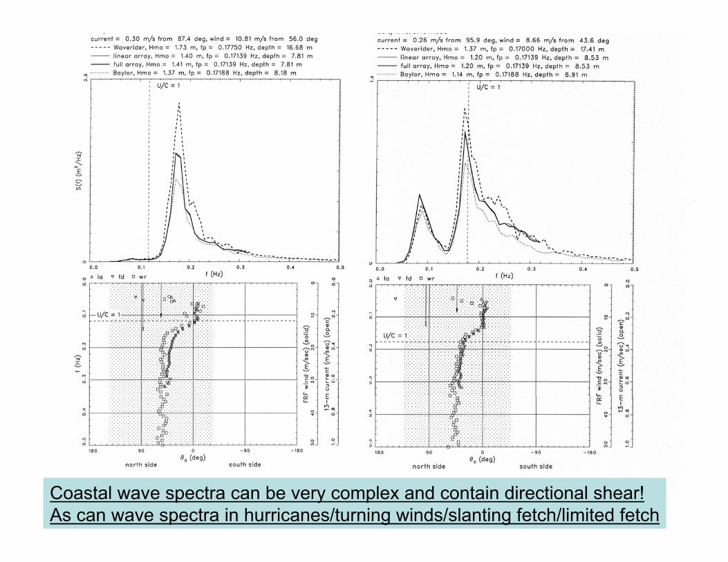
Coastal wave spectra are very complex!Coastal wave spectra can be very complex and contain directional shear!As can wave spectra in hurricanes/turning winds/slanting fetch/limited fetch

Even “simple” spectra can have relatively complex shapes!

AnalysesFrom LongAnd Resio2006 JGR

11 3 3

( ) ( , ) n k T k k dkt

∂=

∂ ∫∫

11 3 1 3 4 2 2 4 3 1 1 2 3 4( , ) [ ( ) ( )] ( , , , ) | |WT k k n n n n n n n n C k k k k ds

n−∂

= − + −∂∫

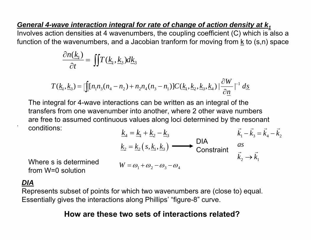
General 4-wave interaction integral for rate of change of action density at k1Involves action densities at 4 wavenumbers, the coupling coefficient (C) which is also afunction of the wavenumbers, and a Jacobian tranform for moving from k to (s,n) space

The integral for 4-wave interactions can be written as an integral of the transfers from one wavenumber into another, where 2 other wave numbersare free to assumed continuous values along loci determined by the resonantconditions:

Where s is determinedfrom W=0 solution

4 1 2 3k k k k= + −

( )2 2 1 3, ,k k s k k=

,

1 2 3 4W ω ω ω ω= + − −

DIARepresents subset of points for which two wavenumbers are (close to) equal. Essentially gives the interactions along Phillips’ “figure-8” curve.

How are these two sets of interactions related?

1 3 4 2

2 1

k k k kas

k k

− = −

→

r r r r

r rDIAConstraint

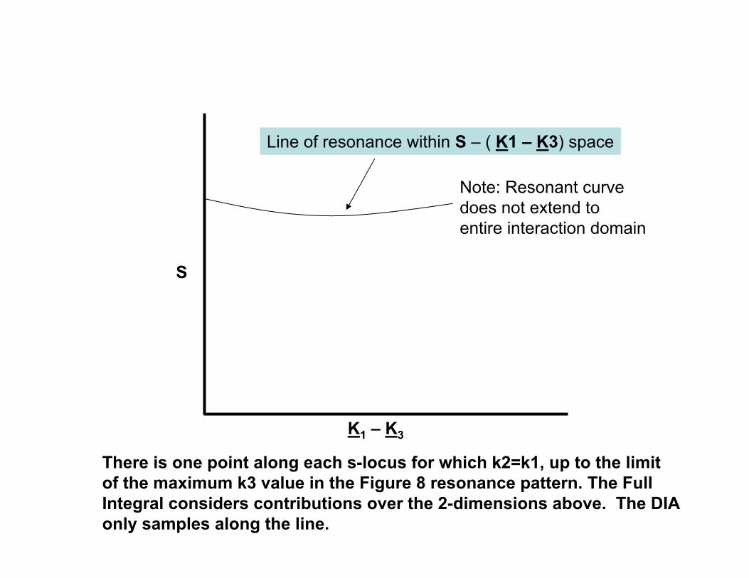
K1 – K3

S

Note: Resonant curvedoes not extend toentire interaction domain

Line of resonance within S – ( K1 – K3) space

There is one point along each s-locus for which k2=k1, up to the limitof the maximum k3 value in the Figure 8 resonance pattern. The FullIntegral considers contributions over the 2-dimensions above. The DIAonly samples along the line.

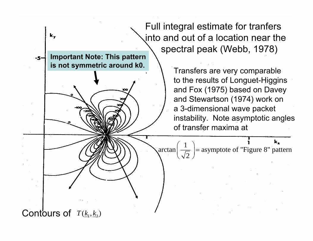
Full integral estimate for tranfersinto and out of a location near the

spectral peak (Webb, 1978)

. Transfers are very comparableto the results of Longuet-Higgins and Fox (1975) based on Daveyand Stewartson (1974) work ona 3-dimensional wave packetinstability. Note asymptotic anglesof transfer maxima at

1arctan asymptote of "Figure 8" pattern2

⎛ ⎞ =⎜ ⎟⎝ ⎠

1 3( , )T k kContours of

Important Note: This patternis not symmetric around k0.

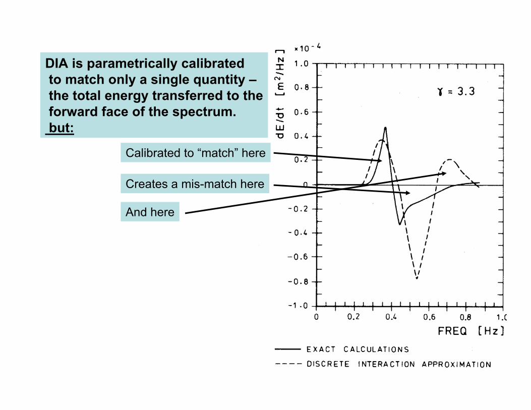
Calibrated to “match” here

Creates a mis-match here

And here

DIA is parametrically calibratedto match only a single quantity –the total energy transferred to theforward face of the spectrum.but:

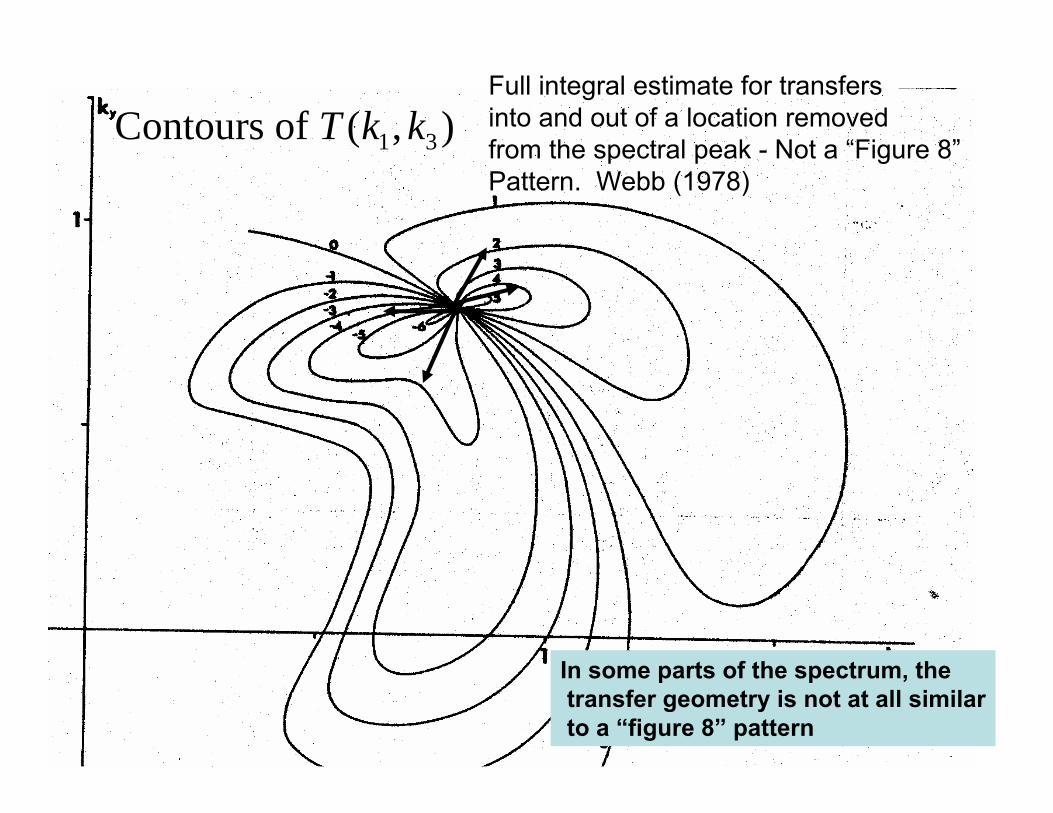
Full integral estimate for transfersinto and out of a location removedfrom the spectral peak - Not a “Figure 8”Pattern. Webb (1978)

1 3Contours of ( , )T k k

In some parts of the spectrum, thetransfer geometry is not at all similarto a “figure 8” pattern

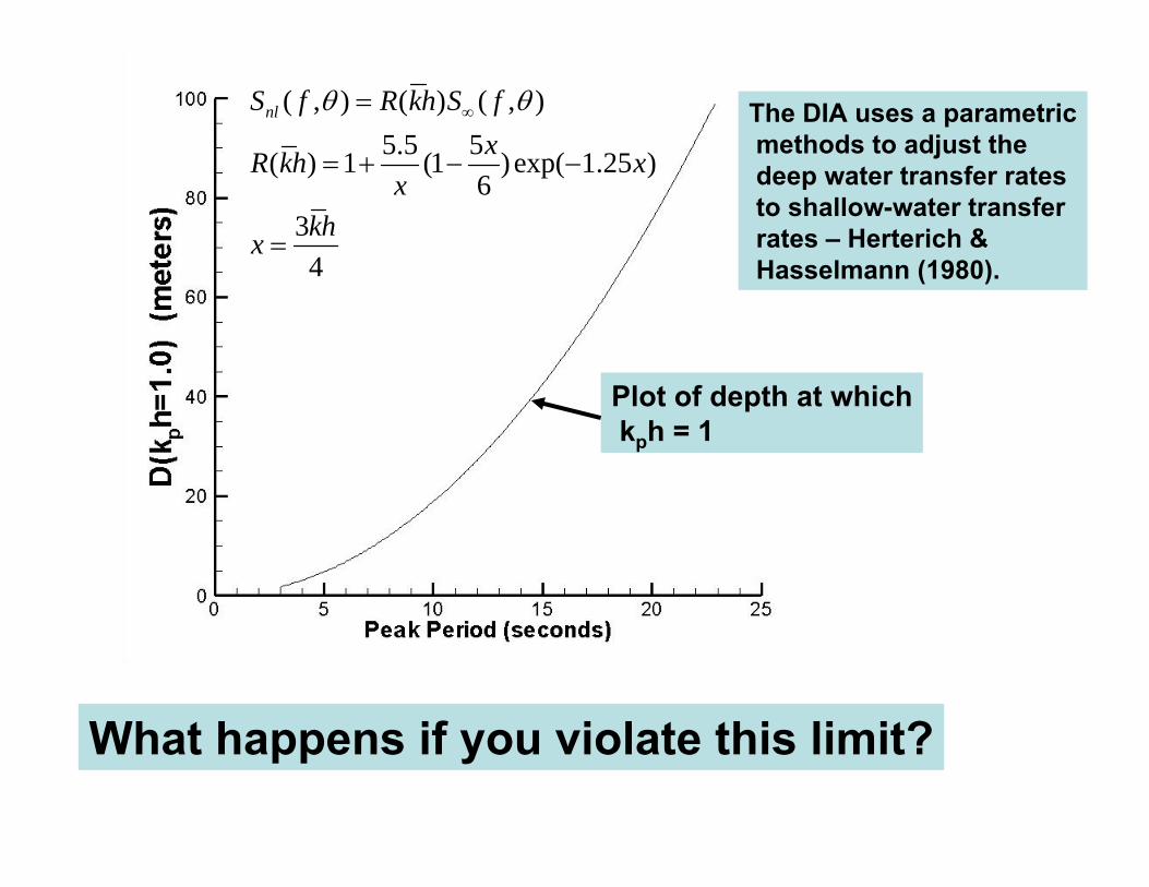
What happens if you violate this limit?

( , ) ( ) ( , )5.5 5( ) 1 (1 )exp( 1.25 )

634

nlS f R kh S fxR kh x

xkhx

θ θ∞=

= + − −

=

Plot of depth at whichkph = 1

The DIA uses a parametricmethods to adjust thedeep water transfer ratesto shallow-water transferrates – Herterich &Hasselmann (1980).

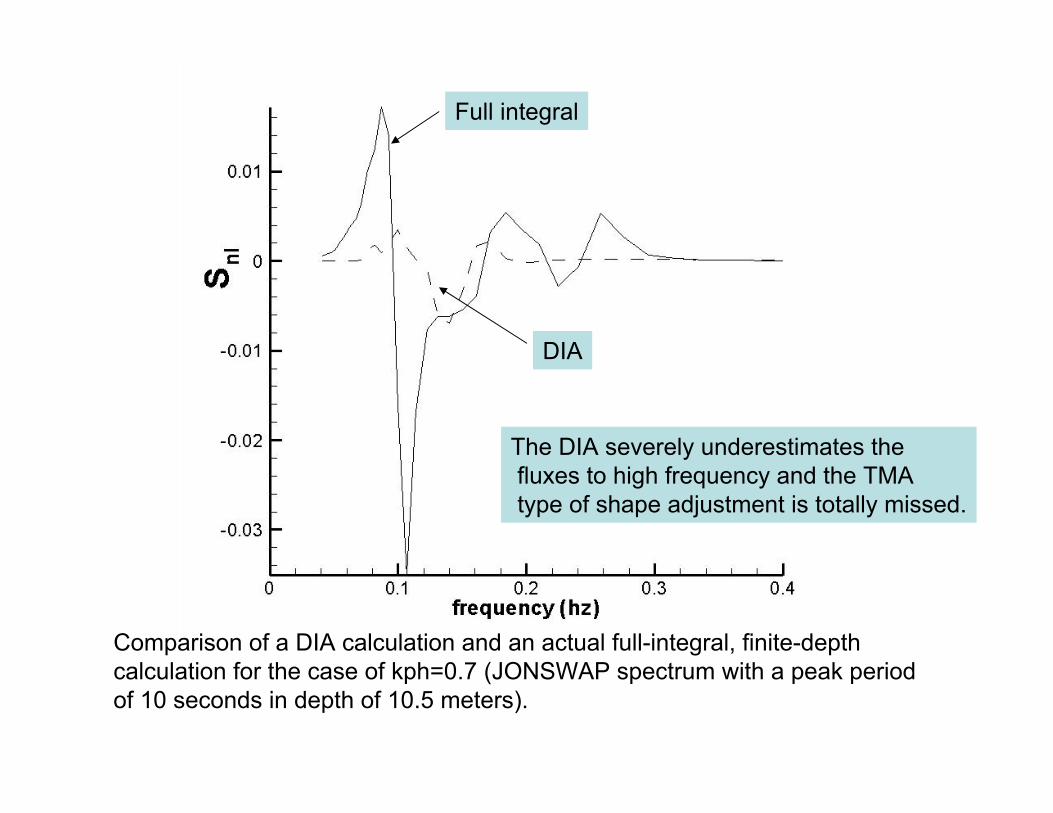
Comparison of a DIA calculation and an actual full-integral, finite-depthcalculation for the case of kph=0.7 (JONSWAP spectrum with a peak period of 10 seconds in depth of 10.5 meters).

Full integral

DIA

The DIA severely underestimates thefluxes to high frequency and the TMAtype of shape adjustment is totally missed.

Since the DIA only samples a slice fromthe complete integral, and is tuned tofit a specific spectrum, how well does itwork for a range of peakedness typicalof wave generation conditions?

Standard JONSWAPγ = 3.3

Standard JONSWAPγ = 1.0

Standard JONSWAPγ = 7.0

DIA performance for JONSWAPspectra with selected peakednessvalues. Solid line is full integral.Dashed line is DIA. This does notprovide a consistent amount of energyto forward face of spectrum.

DIA

Full Integral

The ratio of the maximum value within the positive lobe predicted by the DIA to the maximum value predicted by the full integral, as a function of JONSWAP spectral peakedness parameter, γ.

As the spectrum approaches full developmentthe DIA progressively overpredicts the amountof energy transferred to the forward face of thespectrum – requiring other terms in the detailedbalance to try to compensate for this transfer.

Same as previous figure, defining a ratio for the largest negativevalues within the negative lobe, as a function of JONSWAP spectral peakedness parameter, γ.

Problem with DIA – The basis is not the integral that we aretrying to estimate.

We need a new approximation that;

• conserves constants of motion (action, energy, momentum)• has its basis in the correct integral (important for complex cases)• retains the number of degrees of freedom in the modeled spectrum• is not limited to kph ≥ 1• is much more efficient than the full integral

31 3 4 2 2 4 3 1

1 3 4 2 2 4 3 1

1 3 4 2 2 4 3 1

1 3 4 2 2 4 3 1

1 3 4 2 2 4 3 1

ˆ ˆ ˆ ˆ ˆ ˆ ˆ ˆ( ) ( ) ( ) ( )

ˆ ˆ ˆ ˆ ( ) ( )ˆ ˆ ˆ ˆ ( ) ( )

ˆ ˆ ˆ ˆ ˆ ˆ ( ) ( )

N n n n n n n n nn n n n n n n nn n n n n n n nn n n n n n n nn n n n n n n n

= − + − +′ ′ ′ ′ ′ ′ ′ ′− + − +

′ ′ ′ ′− + − +′ ′ ′ ′− + − +′ ′− + − +

1 3 4 2 2 4 3 1

1 3 4 2 2 4 3 1

1 3 4 2 2 4 3 1

ˆ ˆ ˆ ˆ ˆ ˆ ( ) ( )ˆ ˆ ( ) ( )

ˆ ˆ ( ) ( )

n n n n n n n nn n n n n n n nn n n n n n n n

′ ′− + − +′ ′ ′ ′ ′ ′− + − +

′ ′ ′ ′ ′ ′− + −

ˆ

( , )nl

n n n

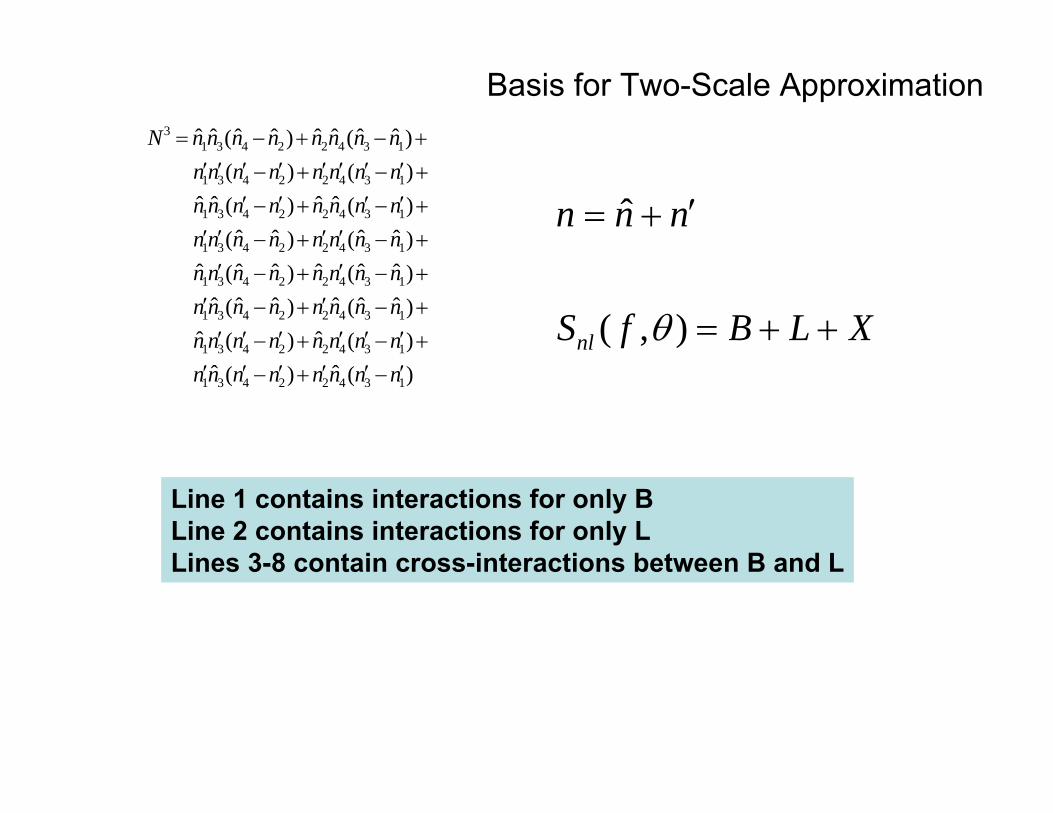
S f B L Xθ

′= +

= + +

Contains both L and X terms

Basis for Two-Scale Approximation

Line 1 contains interactions for only BLine 2 contains interactions for only LLines 3-8 contain cross-interactions between B and L

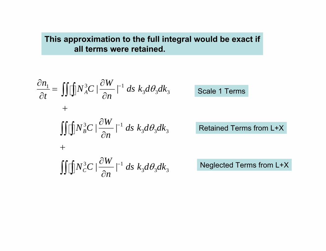
3 113 3 3

3 13 3 3

3 13 3 3

| |

| |

| |

A

B

C

n WN C ds k d dkt n

WN C ds k d dkn

WN C ds k d dkn

θ

θ

θ

−

−

−

∂ ∂=

∂ ∂+

∂∂

+∂∂

∫∫ ∫

∫∫ ∫

∫∫ ∫

Scale 1 Terms

Retained Terms from L+X

Neglected Terms from L+X

This approximation to the full integral would be exact ifall terms were retained.

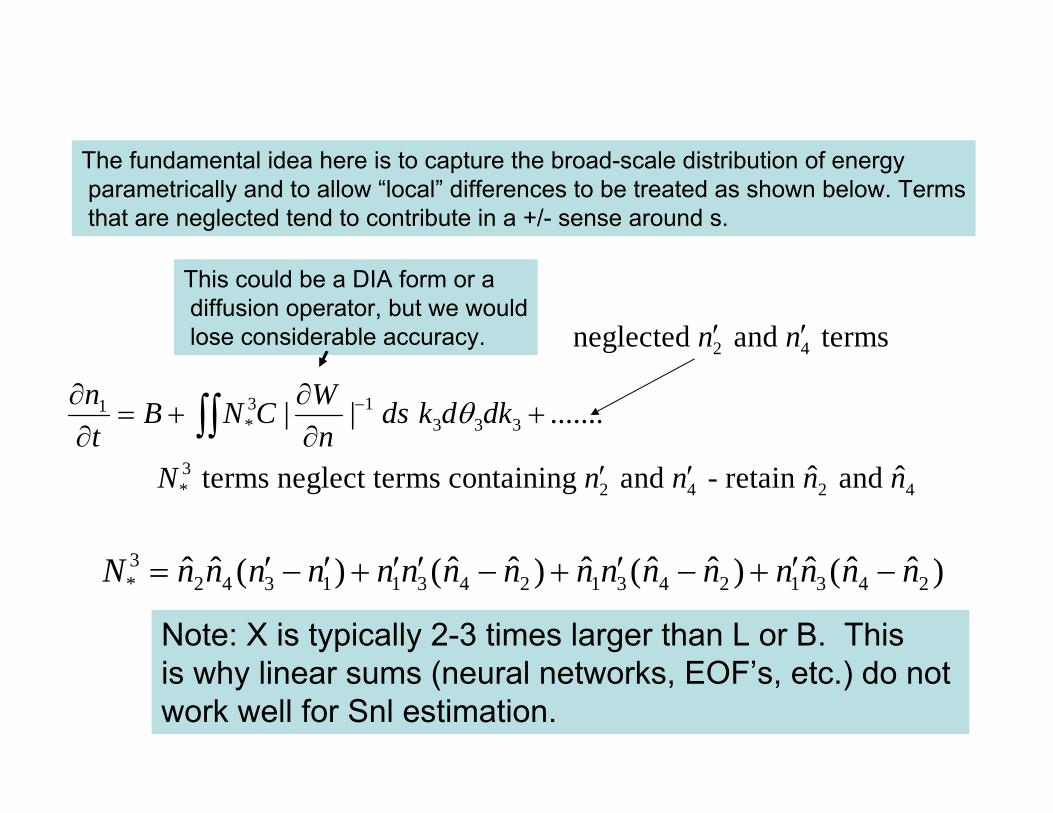
3 11* 3 3 3| | .......n WB N C ds k d dk

t nθ−∂ ∂

= + +∂ ∂∫∫

3* 2 4 2 4ˆ ˆ terms neglect terms containing and - retain and N n n n n′ ′

3* 2 4 3 1 1 3 4 2 1 3 4 2 1 3 4 2ˆ ˆ ˆ ˆ ˆ ˆ ˆ ˆ ˆ ˆ( ) ( ) ( ) ( )N n n n n n n n n n n n n n n n n′ ′ ′ ′ ′ ′= − + − + − + −

Note: X is typically 2-3 times larger than L or B. Thisis why linear sums (neural networks, EOF’s, etc.) do not work well for Snl estimation.

2 4neglected and termsn n′ ′

The fundamental idea here is to capture the broad-scale distribution of energy parametrically and to allow “local” differences to be treated as shown below. Termsthat are neglected tend to contribute in a +/- sense around s.

This could be a DIA form or adiffusion operator, but we wouldlose considerable accuracy.

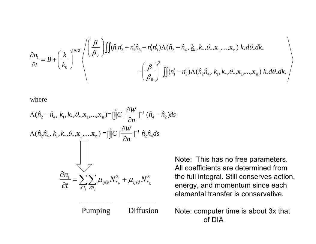
1 3 1 3 1 3 2 4 1 * * 1 n * * *19/ 201

20

1 3 2 4 1 * * 1 n * * *0

2 4 1

ˆ ˆ ˆ ˆ( ) ( , , , ,x ,...,x )

ˆ ˆ ( ) ( , , , ,x ,...,x )

where

ˆ ˆ( , ,

n n n n n n n n k k k d dkn kBt k

n n n n k k k d dk

n n k k

β θ θβ

β θ θβ

⎛ ⎞′ ′ ′ ′+ + Λ −⎜ ⎟

⎛ ⎞ ⎝ ⎠∂= + ⎜ ⎟∂ ⎛ ⎞⎝ ⎠

′ ′+ − Λ⎜ ⎟⎝ ⎠

Λ −

∫∫

∫∫

1* * 1 n 4 2

12 4 1 * * 1 n 2 4

ˆ ˆ, ,x ,...,x )= | | ( )

ˆ ˆ ˆ ˆ( , , , ,x ,...,x ) = | |

WC n n dsn

Wn n k k C n n dsn

θ

θ

−

−

∂−

∂∂

Λ∂

∫

∫

Note: These terms arepre-calculated. Thisremoves all calculationsfrom innermost loopin the integration.

3 31* *

________ _______ Pumping Diffusion

P D

i j

ijsp ijsdf

n N Nt δ δθ

µ µ∂= +

∂ ∑∑ r r All coefficients are determinedFrom pre-calculated integrals

Note: This has no free parameters.All coefficients are determined fromthe full integral. Still conserves action,energy, and momentum since eachelemental transfer is conservative.

Note: computer time is about 3x thatof DIA

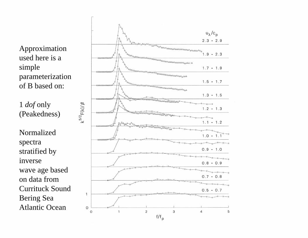
Approximation used here is a simple parameterization of B based on:

1 dof only(Peakedness)

Normalized spectrastratified by inversewave age basedon data from Currituck SoundBering SeaAtlantic Ocean

Note f-5 region in all spectral groups

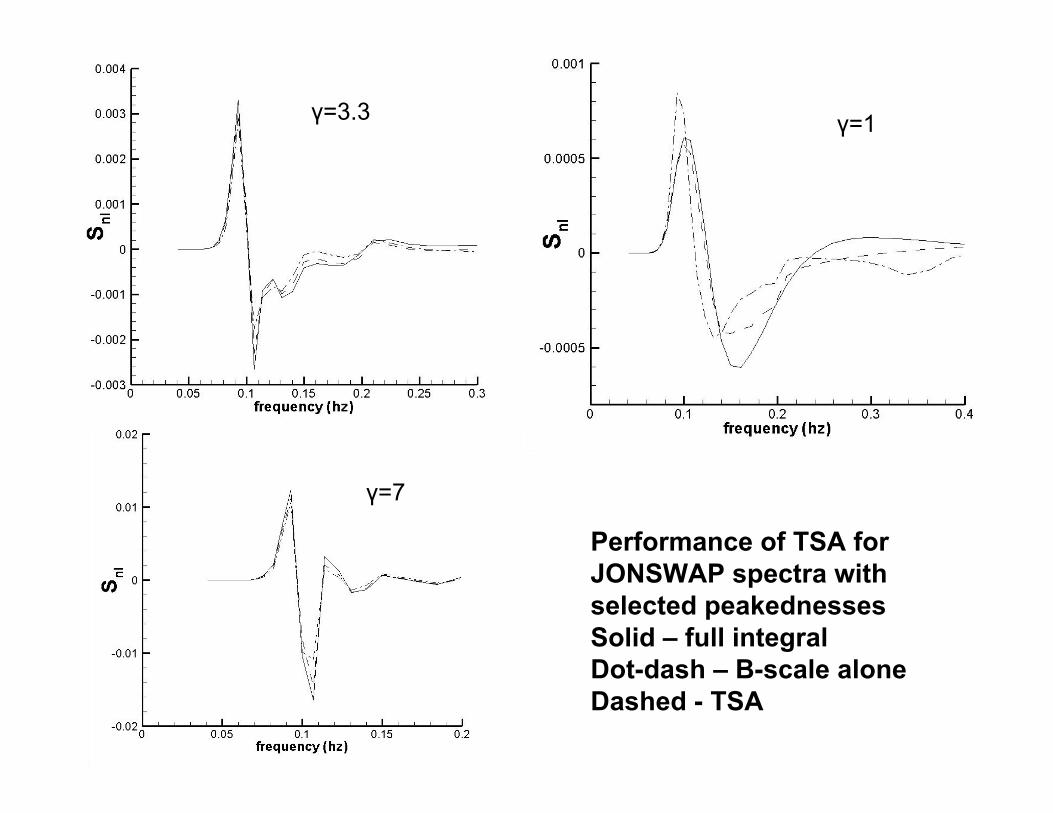
Performance of TSA forJONSWAP spectra with selected peakednessesSolid – full integralDot-dash – B-scale aloneDashed - TSA

γ=3.3 γ=1

γ=7

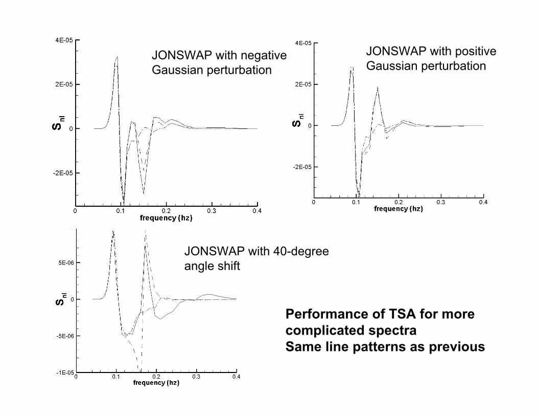
JONSWAP with negativeGaussian perturbation

JONSWAP with positiveGaussian perturbation

JONSWAP with negativeGaussian perturbation

JONSWAP with 40-degreeangle shift

Performance of TSA for morecomplicated spectraSame line patterns as previous

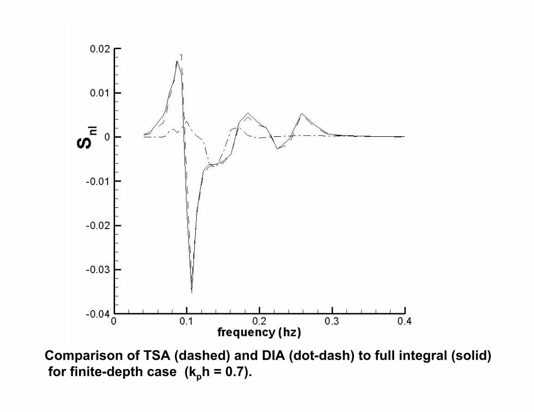
Comparison of TSA (dashed) and DIA (dot-dash) to full integral (solid)for finite-depth case (kph = 0.7).

Example of actual spectrum with crude parameterization.In this case, the spectral shape is highly variable in terms of itsangular distribution and the peak shape is not well approximated.

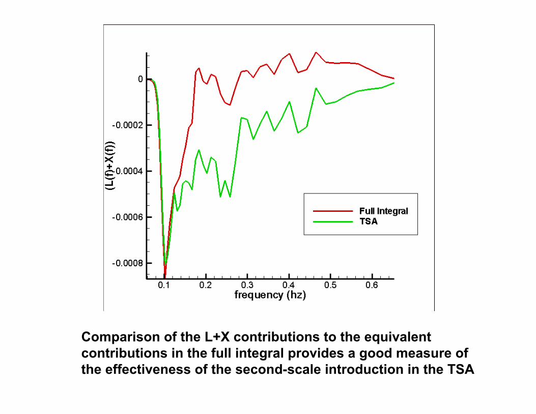
Comparison of the L+X contributions to the equivalent contributions in the full integral provides a good measure ofthe effectiveness of the second-scale introduction in the TSA

The TSA

• conserves constants of motion (action, energy, momentum)• has its basis in the correct integral (important for complex cases)• retains the number of degrees of freedom as the modeled spectrum• is not limited to kph ≥ 1

AND

• is much more efficient than the full integral

Number of mathematical operations is

about 3xDIA for 1 quadraplet (about 1.5 if two sets of q’s are used)BUT: DIA’s instability makes it unstable for moderate time steps!

about 1/250 of the time of the Full Integral

CONCLUSIONS

• DIA has extreme difficulty in reproducing Snl since it does not represent the full set of 4-wave interactions.

• Although DIA is calibrated to provide similar energy transfer to theLow-frequency region of the spectrum, the calibration is only locally valid (near γ=3.3).

• The parametric extension of the DIA to shallow water does notcapture essential elements of nonlinear energy fluxes and their effects on spectral shape in coastal waters

• The TSA appears to be a more accurate alternative to the DIA forboth deep water and shallow water cases

• The initial TSA can be extended to improve the B-scale treatment which should improve its accuracy for operational applications.