The Unequal Effects of Liberalization: Theory andEvidence from India∗

Philippe Aghion† Robin Burgess‡ Stephen Redding§

Fabrizio Zilibotti¶

October 3, 2003

Abstract

This paper exploits the 1991 Indian liberalization to illustrate how sucha reform may have unequal effects on industries and regions within a singlecountry. We begin by developing a Schumpeterian growth model to analyzethe effects on industrial performance of liberalization reforms aimed at increas-ing entry. The main predictions of the model are: (i) liberalization enhancesproductivity, investment, profits and output, in industries that are initiallyclose to the technological frontier, while it has the reverse effect in industrieswhich are initially far below the frontier; (ii) pro-worker labor regulations dis-courage productivity, investment, profits and output in all industries and thisnegative effect is magnified by liberalization. We test these predictions in a 3-digit industry panel data set for the sixteen main states of India over the period1980-1997. The empirical results confirm the main predictions of the model.We find that the 1991 liberalization in India had strong inequalizing effects,by fostering productivity and output growth in 3-digit industries that were ini-tially closer to the Indian productivity frontier and which were located in stateswith more pro-employer labor institutions. These findings emphasize that theinitial level of technology and institutional context mattered for whether andto what extent state-industries in India benefited from liberalization.

∗We are grateful to Timothy Besley, Elhanan Helpman and seminar participants at the CanadianInstitute for Advanced Research and UCL for useful comments and suggestions. Juan Pablo Rudand Kwong Tok Soo provided excellent research assistance. We thank the CEPR, Leverhulme Trustand STICERD, LSE for financial support.

†Harvard University and CEPR‡LSE, BREAD and CEPR§LSE and CEPR¶IIES and CEPR

1

1 Introduction

Globalization and its effects on economic development have been the subject of anintense and passionate debate over the last decade. The optimistic view argues thattrade liberalization, and the implied elimination of barriers to competition, is theright road for developing countries to promote growth and eradicate poverty (see, forexample, Dollar and Kray (2001, 2002), Frankel and Romer (1999), Sachs and Warner(1995) and World Bank (2001)). Skeptics object that there can be no such progresswithout an active role for domestic institutions and policies to correct market failures(Rodrik and Rodriguez (2000), Rodrik et al. (2002)), and argue that liberalizationmay even be detrimental to growth, by inhibiting infant industries and the localaccumulation of knowledge (Krugman (1981), Haussman and Rodrik (2002), Young(1991), Stiglitz (1995, 2002).This paper intends to contribute to this debate from both a theoretical and an

empirical standpoint, providing a unifying framework to discuss the effect of global-ization on growth and inequality. We analyze how trade liberalization interacts withpre-reform technological capability and domestic institutions in affecting industrialperformance. As a result the effect of the same macroeconomic reform can vary sub-stantially across regions and industries in the same country. Domestic institutionssuch as those governing labor relations will also affect the response of innovativeinvestments to trade liberalization.We formalize these ideas in a simple version of a Schumpeterian growth model

with entry threat that we use to guide our empirical research. We formulate and testtwo main implications of the theory.First, a liberalization reform introducing trade liberalization should give rise to

larger increases in productivity, investment, rents and output in state-industries thatare closer to the frontier. The growth-enhancing effect should be smaller, and possiblynegative, in firms and sectors that are farther from frontier. The reason is thatincumbent firms that are sufficiently close to the technological frontier can surviveor deter entry by innovating. An increased entry threat, thus, results in higherinnovation intensity aimed at escaping that threat. On the other hand, firms andsectors that are far below the frontier are in a weaker position to fight external entry.For these firms, an increase in the entry threat reduces the expected payoff frominnovating, since their expected life horizon has become shorter.Second, more pro-worker (pro-employer) labor market regulations reduce (in-

crease) productivity, investment, rents and output, and these effects are strengthenedpost-liberalization. More precisely, our theory predicts that the response of innova-tive investments to trade liberalization is dampened in states with more pro-workerlabor regulations. In other terms, the anti-innovative effect of pro-workers regulationsis less pronounced in less competitive environments. Thus, in relative terms, tradereforms hurt growth in regions with pro-labor regulations, while enhancing growth inregions with pro-employer regulations.

2

The empirical analysis focuses on the effects of a recent liberalization episodein India. India underwent a massive reform in 1991 which involved slashing tariffs,deregulating entry and opening up different industrial sectors to foreign direct in-vestment. This episode, which is described in more detail below, represents, for itssize and impact, an attractive experiment to assess the validity of the theory. Moreprecisely, we construct a three-dimensional panel for the period 1980 to 1997 using“Annual Survey of Industries” (ASI) data with variations over 3-digit industry, stateand time. The available data include productivity, investment, rents and output foreach industry-state-time observation.We use a measure of output per worker in the period just before liberalization

(relative to the most productive state-industry observation in the same year) as aproxy for the distance to frontier for a particular 3-digit state-industry. We theninteract this variable with a reform measure which is zero before 1991 and takes ona value of one thereafter to test whether the distance to frontier prior to reform in-fluences the post-reform performance. We first document the effects of the reform onlabor productivity, and then consider separately the effects on total factor produc-tivity, profitability, investment, employment and output. This provides a test of thefirst prediction of the theory, namely that firms closer to the frontier respond morepositively to the threat of entry introduced by liberalization.Second, we consider state-specific labor market regulations. To this aim, we use a

measure of the direction of labor regulation constructed by Besley and Burgess (2003),who coded state amendments to the Industrial Dispute Act of 1947 as pro-labor, neu-tral or pro-capital. We look first at whether the direction of labor regulation acrossthe 1980-1997 period affected industrial performance at the 3-digit state-industrylevel. The level of this variable in 1990, which captures the pre-reform relative bar-gaining powers of workers and employers, is then interacted with the reform dummyand used as an explanatory variable in regressions for profitability, investment, em-ployment and output. The estimated coefficient on this interaction term provides aninference on whether labor regulation in a state at the time of reform affected theperformance of 3-digit state-industries post-liberalization.The regression analysis vindicates the two key predictions of the theory. First,

state-industries that are closer to the technological frontier have indeed experiencedlarger increases real productivity, investment, rents and output in the post-reformperiod. Second, pro-worker labor regulations had a negative effect on the growth ofthe same variables, and this effect was magnified by liberalization. Both results holdtrue after controlling for 3-digit state-industry fixed effects, year dummies and 3-digitindustry time trends.Data on patents taken out by Indian manufacturing firms with the US Patent

Office shows that this form of innovative activity increases in after liberalization andthe increase is greater in state-industries which were closer to the Indian technologicalfrontier pre-reform. state-industries closer to the Indian technological frontier pre-reform. Though this is a somewhat restrictive measure of innovation we find similar

3

results for broader measures of investment which together suggest a non-negligible rolefor innovation. Using a panel of firms which exist in both 1994 and 1997 we also showthat the bulk of the productivity improvement that occurred in the post-liberalizationperiod can be accounted for by within firm productivity improvements with only smallamount coming from reallocation of labor from less to more productive firms. Thoughthis may in part reflect the specificities of the Indian institutional environment (e.g.limitations on closing firms and firing workers) it does suggest that the innovationresponse of incumbent firms to the entry threat posed by liberalization is a large partof the story.Our paper relates to different strands of literature. There is first a theoretical

literature on trade, productivity and growth. Of particular relevance for our empiricalanalysis in this paper, is the recent model by Melitz (2003). In Melitz (2003), tradeliberalization induces a process of reallocation of resources across heterogeneous firms.High productivity firms react to liberalization by incurring some additional fixedcosts to enter foreign markets as they find it optimal to expand their activity inequilibrium. Low productivity firms, in contrast, exit.1 On average, profits andproductivity increase, although there is no productivity change at the firms level.Thus a common feature between Melitz and our model, is that in both cases high-productivity firms stand better chance to resist the a more competitive environment,whereas low productivity firms more often succumb and exit, so that liberalizing entryshifts the firm distribution towards more productive firms. However, in addition tothis “reallocation” effect, in our model liberalization reforms also affect innovationincentives and productivity growth at the firm level. Our empirical analysis confirmsthat this is an important part of the story in India.The evidence gathered so far in the debate on globalization and development is

mainly at the country level and does not arrive at any clear consensus. A contributionof this paper is to look at how an important liberalization episode affected industrialperformance at the microeconomic level. It thus forms part of a literature which ismoving in this direction. Other empirical studies that document the effect of tradeliberalization on productivity growth at the firm or industry level, include Hanson(1997), Harrison (1994), Krishna and Mitra (1998), Levinsohn (1999), Pavcnik (2002),Trefler (2001) and Tybout et al. (1991). Our innovation is to look at the interplaybetween market reforms, institutions and technological development. As is confirmedin the data there is a strong link between liberalization, the technological choices offirms and growth which has recieved limited attention in the literature. A recentpaper by Aghion et al (2003) also pushes in this direction by looking at the effects ofentry on innovation and productivity growth in UK firm level data.On a more general level, our contribution relates to a recent stream of literature

on endogenous growth which emphasizes how policies may have different effects at

1Thus, while in Melitz’ model it is the opportunity to access foreign markets that induces high-productivity firms to invest in foreign market access, in our model firms respond to the threat ofoutside entry by investing resources to increase productivity and thereby escape the entry threat.

4

different stages of the process of technological convergence. This includes Acemoglu,Aghion and Zilibotti (2002) and Aghion et al (2001).2 It also relates to the recentliterature on institutions and development (e.g Acemoglu, Johnson and Robinson(2001, 2002a, 2002b), Banerjee-Duflo (2001), Besley and Burgess (2000, 2003), Halland Jones (1999), La Porta et al. (1998, 1999)).The paper is organized as follows. Section 2 provides background on the Indian

liberalization experiment and on patterns of industrial performance and institutionalchange. Section 3 outlines the theoretical framework and then derives our mainpredictions on how the effects of trade liberalization on performance should dependupon technological and institutional characteristics of industries and states. Section3 confronts these predictions with Annual Survey of Industries data from India andpresents our main empirical findings. Section 4 performs a few robustness tests andcontrasts the results with the predictions of the neo-classical trade model. Section 5concludes.

2 Background

1991 brought to a close a long era of socialist policies in India. Political analysissuggests that the size and scope of the liberalization reforms which ensued were largelyunexpected. Up to this point central government control over industrial developmentwas maintained through public ownership, licensing and other controls. And plannedindustrialization took place in highly protected environment which was maintained byhigh tariff, non-tariff barriers and controls on foreign investment. The New IndustrialPolicy, introduced in 1991 in the wake of a balance of shattered this old order. Tradeliberalization and deregulation were central elements.Using 6-digit industry data from the UN Trade Analysis and Information Systems

Data Base, we find that the average percentage point reduction in tariffs across the1990-1997 period was 51%, with 97% of products experiencing tariff reductions. Thisrepresented one of the most dramatic trade liberalizations ever attempted in a devel-oping country. As part of the liberalization process, the system of import licensingwas also radically reformed, with quantitative controls largely eliminated on importsof intermediate products leading to a rise in the ratio of imports to gross outputoccurring from 1991 onwards.The New Industrial Policy also opened a large number of industries for automatic

approval of foreign technology agreements and to foreign investment of up to 51%

2Aghion et al (2001) analyzes the interplay between innovation and product market competition,and shows that product market competition encourages innovations mostly in “neck-and-neck” sec-tors where most firms are already close to the technological frontier, whereas it discourages innova-tions in sectors where innovating firms are far below the frontier. Acemoglu et al (2002) emphasizesthe idea that different policies or institutions can be growth-enhancing depending upon a country’sor sector’s distance to the technological frontier. In contrast, this paper emphasize asymmetriceffects of trade liberalization across industries and regions in the same economy.

5

of equity. A Foreign Investment Promotion Board was also established to considerproposals of up to 100% equity. These policy reforms were followed by a dramaticrise in the number of approvals of foreign collaboration and actual foreign directinvestment flows showed a similar marked increase.Dramatic deregulation also ensued with the large-scale removal of industrial li-

censing. Under the Industries (Development and Regulation) Act of 1952, firms wererequired to apply for an industrial license from a Licensing Committee in order toset up a new production unit, expand capacity by more than 25% of existing levelsor manufacture a new product. These requirements were removed for the majorityof industrial sectors in 1991. Similarly, the New Industrial Policy saw a substantialreduction in the number of industrial categories reserved for the public sector from17 to 8 in 1991 and to 6 in 1993.Overall liberalization in 1991 has had a positive impact on registered manufac-

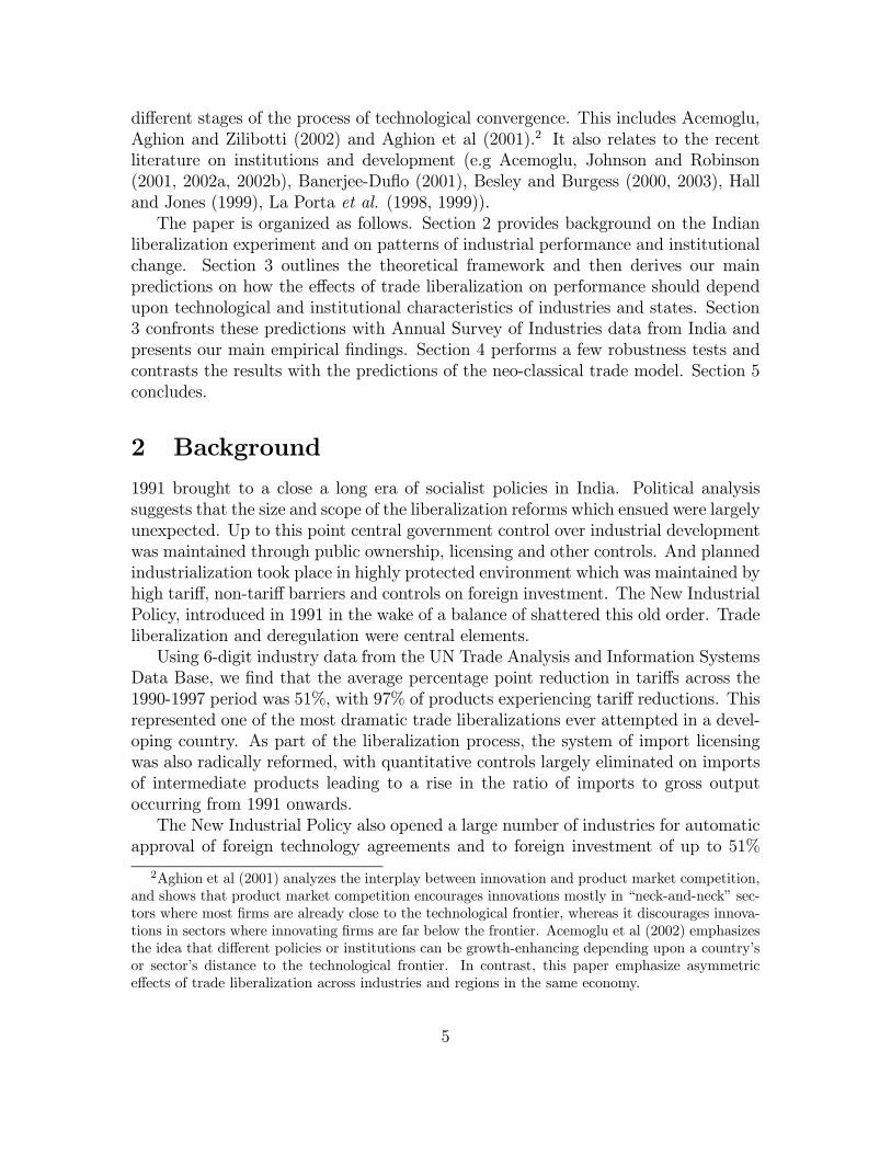
turing — whereas the growth rate of real per capita manufacturing was around 4% inthe 1960-1991 period this jumped to about 7% in the 1991-1997 period. This patterngives some support to those who see globalization as having a net positive impact oneconomic performance. Figure 1 graphs out per capita real registered manufacturingoutput in the sixteen main Indian states for the period 1980 to 1997. Our focus is onregistered manufacturing which covers firms with more than 10 employees with poweror more than 20 employees without. It is these firms that are covered in the AnnualSurvey of Industries and which have been subject to the labor and planning regula-tions. What is striking about Figure 1 is the fact that manufacturing performancevaries so strongly across states and that there is a clear divergence in performancepost-1991. This marked heterogeneity in responses to a common liberalization shockin the same country is something which we will explore in our theoretical framework.And it gives support to those who believe that globalization is not uniformly bene-ficial and that institutional and other conditions matter a lot for whether a firm orindustry will benefit. Understanding what institutional and policy choices are con-ducive to a country or region benefiting from liberalization is an open and importantquestion.Moreover if we dig further we find that productivity levels pre-reform in the same

3-digit industry varied strongly across Indian states. As a result, the same industriesin different states were at different distances to the Indian technological frontier. Wecan exploit this fact to examine whether distance to frontier pre-reform mattered forpost-liberalization performance. This has important implications for understandingthe impact that liberalization has on incentives for firms to adopt new technologyand make investments that increase productivity.Divergent manufacturing performances across Indian states in the post-91 period

is likely to have contributed to growing inequality. We examine this issue in Figure 2where we graph out the standard deviation of real manufacturing output per workerfor each year across the period 1980 to 1997. Whereas differences across states inoutput were falling in the 1980-1991 period this trend changed direction in this year

6

and we see growing inequality in productivity across after 1991. Liberalization doesindeed seem to have had unequal effects on industrial performance across the 1980-1997 period.We also exploit the fact that India is a federal democracy which implies that differ-

ent states have made different institutional and policy choices. Tax and expenditurepowers of central and state governments are listed in the Indian Constitution (theUnion and State Lists). A third list — the Concurrent List — covers areas where thecentral and state governments have joint jurisdiction. Industrial relations falls on thislist. States therefore have the power to amend central legislation in this area. We usethe coding by Besley and Burgess (2003) of all state level amendments to the Indus-trial Disputes Act of 1947 to capture industrial relations climate in a state. Besleyand Burgess (2003) read the text of each state level amendment (121 in all) and codedeach one as either being neutral (0), pro-worker (1) or pro-employer (-1).3 In years inwhich there were multiple amendments, an indicator of the overall direction of changewas used. So, for example, if there were four pro-worker amendments in a given stateand year, this was coded as plus one rather than plus four. Having obtained the netdirection of amendments in any given year, the scores were cumulated over time togive a quantitative picture of the evolving regulatory environment.Coding the measure this way gives us both cross-state and time series variation.4

The measure captures the extent to which can workers appropriate industrial rents.This may affect the incentives for incumbent firms to make innovative investments as aresponse to entry threats. From Besley and Burgess (2003) we know that the directionof labor regulation is a key determinant of registered manufacturing performance atthe state level for period 1958-1992. In this paper we want to exploit this measure toexamine whether the pre-reform industrial relations climate in a state affected post-reform performance at the 3-digit industry level. In particular, we want to examinewhether the response of innovative investment to trade liberalization is dampened instates with more pro-worker labor market institutions.The labor regulation measure is displayed in Figure 3. It is clear that the states

of India divide into “treatment” and “control” groups. The latter are states thatdo not experience any amendment activity in a pro-worker or pro-employer directionover the 1958-1997 period. There are six of these: Assam, Bihar, Haryana, Jammu &Kashmir, Punjab and Uttar Pradesh. Among those that have passed amendments, sixstates are classified as “pro-employer”: Andhra Pradesh, Karnataka, Kerala, MadhyaPradesh, Rajasthan and Tamil Nadu. Four are classified as “pro-worker”: Gujarat,Maharashtra, Orissa and West Bengal.Taken together, the stylized facts reviewed in this section confirm that, though

3Summaries of all amendments and their coding is available athttp://econ.lse.ac.uk/staff/rburgess/#wps.

4Using an institutional measure within a country also helps us to abstract from concerns withunobserved heterogeneity and omitted variables which afflict cross-country studies of institutionsand growth.

7

liberalization had an overall positive effect on industrial performance, its effects werehighly unequal across Indian states and industries. We now turn to building a the-oretical framework which allow us to look at the interactions between liberalization,the technological capability of firms and industries, institutional environment andindustrial performance.

3 Theoretical framework

In this section we develop a discrete-time Schumpeterian growth model with productentry. This allows us to capture how an economy-wide liberalization which lowersbarriers to entry can affect the investment decisions of firms and thereby their pro-ductivity and output. The focus of our analysis is on how initial technological devel-opment, which differs across industries, and local institutions (e.g local labor marketconditions), which differ across states, mediate this relationship between liberalizationand industrial performance. The main prediction of our model is that liberalization,modeled as an exogenous shock on the probability of product entry to capture theIndian liberalization experiment, affects output and productivity growth differently,both, across industries with different initial levels of technology and across stateswhere the allocation of productive surplus between employers and workers varies.Liberalization thus leads to a widening in the productivity and output distributionsas the performance of firms and industries closer to pre-reform technological frontierand located in states with pro-employer labor institutions improves whilst the per-formance of their counterparts far from the frontier and located in pro-worker statesdeclines.

3.1 The environment

Our description of the basic environment builds upon Acemoglu et al (2002), whichwe adapt to the case of an economy consisting of a set of “states” (or regions) whichdiffer in their factor endowments, distribution of productivities across firms and labormarket regulations.All agents live for one period. In each period t a final good (henceforth the

numeraire) is produced in each state by a competitive sector using a continuum oneof intermediate inputs, according to the technology:

ys,t =1

α[Z 1

0(As,t (ν))

1−αxs,t (ν)α dν].

xs,t (ν) is the quantity of intermediate input produced in sector ν, state s and datet, As,t (ν) is a productivity parameter that measures the quality of the intermediateinput ν in producing the final good, and α ∈ (0, 1). The final good can be used eitherfor consumption, or as an input in the process of production of intermediate goods,

8

or for investments in innovation. For simplicity, we drop the state index s when thisis not a source of confusion.In each intermediate sector ν only one firm (a monopolist) is active in each period.

Thus the variable ν refers both, to an intermediate sector (industry), and to theintermediate firm which is active in that sector. As any other agent in the economy,intermediate producers live for one period only and property rights over intermediatefirms are transmitted within dynasties. Intermediate firms use labor and capital (finalgood) as inputs, according to the following Cobb-Douglas technology:

xt(ν) = kβt (ν)l

1−βt (ν),

where kt(ν) and lt(ν) denote the amounts of labor and capital inputs to produce xt(ν)units of intermediate input.The monopoly power of intermediate producers is limited by the existence of a

competitive fringe of firms that can produce one unit of the same intermediate inputusing χ units of final good, with χ < 1

α. Given the potential competition from the

fringe, it is optimal for the intermediate good producer to charge the limit price

pt (ν) = χ (1)

for each unit of the intermediate good ν sold to the final good sector. In equilibrium,the competitive fringe will not be active.5

Since the final good sector is competitive, the equilibrium price of each interme-diate input, ν, must equal its marginal productivity in the final good sector, namely:

pt (ν) = (At (ν) /xt (ν))1−α. (2)

Equating (2) to (1) implies that, in equilibrium,

xt(ν) = At (ν)χ− 11−α .

We assume that each state authority imposes a minimum wage (wt), identicalacross firms. This assumption is meant to capture not so much wage rigidity butrather, and in a reduced form way, the effect of labor market regulations which affectthe relative bargaining power of employers and workers, and therefore workers’ abilityto extract the surplus generated by firms.6

5The existence of a competitive fringe that forces monopolist to charge a limit price is introducedfor tractability. If firms could charge the unconstrained monopoly price, the analysis would beconceptually similar, but more involved.

6An alternative approach would have been to explicitly model the bargaining process betweenfirms and workers, using a framework a la Stole-Zwiebel (1995) to formalize the bargaining gamebetween each firm and its multiple workers, but extending the analysis to an economy with het-erogeneous firms. Characterizing the general equilibrium outcome (with unemployment) in such anenvironment, introduces a number of complications which are largely orthogonal to the effects weare pointing out in this paper.

9

The minimum wage is assumed to be binding, i.e., to be higher than the market-clearing wage. This implies that, in all states, there is excess supply of labor at thegoing wage. Workers who cannot find employment in the manufacturing sector areeither unemployed or employed in a residual informal sector.In equilibrium, profits in each intermediate firm, ν, are then simply equal to:

πt (ν) = maxk(ν),l(ν)

χkt (ν)β lt (ν)1−β − kt (ν)− wtlt (ν)

s.t : kt (ν)β lt (ν)

1−β ≥ xt(ν) = At (ν)χ− 11−α .

Straightforward maximization yields:

lt(ν) = At (ν)χ− 11−α

Ãβ

1− βwt

!−β; (3)

kt(ν) = At (ν)χ− 11−α

Ãβ

1− βwt

!1−β, (4)

and, therefore:πt(ν) = At (ν) δ (wt) , (5)

where

δ (wt) ≡ χ−1

1−α³χ− w1−βt β−β(1− β)−(1−β)

´and, hence, profits are decreasing functions of the state-specific wage, wt, and of theextent of potential competition (i.e., the inverse of χ).Substituting for xt(ν) in the production function for final output, we get:

yt =1

αχ−

α1−αAt,

where

At =Z 1

0At(ν)dν

is the average productivity in the state.Finally, higher wages imply that firms will choose more capital-intensive tech-

niques. More formally, let κt (ν) = kt(ν)/lt (ν) denote the capital-intensity of theproduction technique. Then, in equilibrium;

κt (ν) =β

1− βwt = κ (wt) . (6)

10

3.2 Technological states, innovation, and entry

3.2.1 Advanced and backward firms

In every period, and within each state, intermediate firms differ in terms of theircurrent distance to the “technological frontier”. We denote the productivity of thefrontier technology at the end of period t by At and assume that this frontier growsat the exogenous rate g7. More formally:

At = At−1 (1 + g) .

At the beginning of period t (or, identically, at the end of period t−1), the leadingfirm in the production of a particular intermediate input can be in two states:

• “advanced” firms have a productivity level At−1 (ν) = At−1, namely, are at thecurrent frontier.

• “backward” firms have a productivity level At−1 (ν) = At−2, namely, are onestep behind the frontier.

Before deciding about their production plans, firms can undertake innovative in-vestments to increase their productivity. Innovative investments have a stochasticreturn. In case of success, the incumbent firm can adopt the next most productivetechnology, that is can increase its productivity by a factor 1 + g and thus keep thepace with the advancement of the technological frontier. The cost of technology adop-tion is assumed to be quadratic in the probability of successful adoption and linearin the current level of technology:

ct (ν) =1

2z2tAt−1 (ν) ,

where z is the probability of success of the innovative investment. If the investmentis not successful (probability 1 − z), instead, the firm produces with a productivitylevel equal to its initial state.We make the following assumptions about firms’ dynamics.8 If an advanced firm

is successful at time t, it starts as an advanced firm at time t + 1. All other firmsstart as backward firms (note that this implies that firms with a realized productivityequal to At−2 at time t automatically upgrade their initial productivity due to animplicit spillover effect). However, with an exogenous probability h, a backwardfirm at the end of period t is replaced by a new firm starting as advanced at time

7In the empirical section the frontier technology refers to the Indian frontier, not the worldfrontier. Our choice there is mainly based on the fact that it is harder to find world (i.e essentiallyUS) equivalents for a number of goods manufactured in India.

8These assumptions are made for the sake of notational simplicity but they do not affect ouranalysis and results in any major way.

11

t + 1. Let at denote the proportion of “advanced” firms at t, and zA,t denote theinnovation intensity of an advanced firm at time t. Then the productivity distributionis characterized by the following dynamic equation:

at+1 = zA,tat + h (1− zA,tat) = (1− h) zA,tat + h,

so that the steady-state proportion of advanced firms is equal to

a∗ =h

1− zA (1− h) .

3.2.2 Entry

Intermediate firms are subject to competition from foreign producers. In particular,we assume that, in every period, a foreign producer can operate a product entry inthe local market for a particular intermediate good. Product entry means that theforeign producer succeeds in selling his product on the local market in the currentperiod, but that she does not permanently replace local producers and therefore shedoes not directly affect the distribution of productivities in the next periods. Thisassumption allows us to formalize the notion of “threat of entry” in the simplest way.9

Foreign firms observe the outcome of the innovative investment of the local firm,and face the following decision. They can either stay out of the market, or pay a smallfixed cost, ζ, and be granted permission to sell in the local market with probabilityµ.10 Foreign entrants at date t are assumed to operate with the end-of-period frontierproductivity, At.If the foreign firm manages to enter and competes with a local firm which has a

lower productivity, it steals all the market. If it competes with a local firms whichhas the same productivity, however, Bertrand competition drives the profits of boththe local and the foreign firm to zero. We assume the parameters to be such thatthe foreign firm will always find it profitable to try to enter if the local firm has aproductivity level lower than the frontier (more formally, we require ζ to be sufficiently

9A first interpretation of the product entry assumption is that entry threat is primarily affectedby the degree of openness to foreign trade; a second interpretation is that product differentiation anda better knowledge of local market conditions, allow local producers to remain in the market afterforeign entry occurs, so that one can analyze how an increase in entry threat affects the dynamicsof productivity within a balanced panel of domestic firms. One can show that the main predictionsof our theory survive if we replace the product entry assumption can be replaced by a straight entryassumption, although at the cost of complicating the model (see Aghion et al (2003)).10We can interpret µ as capturing the easiness for foreign firms and products to enter the Indian

market. A higher µ, therefore reflects any reduction in tariffs or regulations which facilitates foreignentry. In the appendix we develop an extension of this model where the probability of entry isendogeneized, and its equilibrium values for the different types of sectors, depend upon an additionalentry cost parameter. While the equilibrium probability of entry will typically differ across thedifferent types of sectors, a reduction in entry cost will still have the same qualitative effects oninnovation and productivity growth across industries and states, as an increase in µ.

12

small). However, the foreign firm will never enter in period t if the local firm hasachieved the frontier productivity level At.

11 Therefore, the end-of-period probabilityof entry in the market for input ν will be equal to:

• zero, if (i) the local firm ν was initially “advanced” and (ii) it has undertakena successful innovative investment;

• µ, otherwise.

3.2.3 Equilibrium innovation investments

We now consider the decisions of local producers, which initially lie at the currentfrontier (“advanced” producers) or one step behind the current frontier (“backward”producers). Once again, in this model, each intermediate producer corresponds toa different intermediate sector or industry, so the differences between advanced andbackward producers are meant to capture differences in the impact of entry acrossindustries at different initial levels of technological development.Recall that all agents live for one period only, therefore incumbent producers born

at date t maximize the expected profits accruing at the end of the same period t. Thisis a useful simplification that avoids to solve more complicated dynamic problems.Backward firms choose their investment so as to maximize expected profits, as

given by:

maxzδhz (1− µ) At−1 + (1− z) (1− µ) At−2

i− 12z2At−2,

whose solution yields:z = δ (1− µ) g = zB. (7)

Recall that backward firms can only make profits if there is no entry (probability1 − µ). The productivity is At−1 if the investment is successful (probability z) andAt−2 if the investment is not successful (probability 1− z).12Advanced firms choose their innovation investment in order to solve the following

program:

maxzδhzAt + (1− z) (1− µ) At−1

i− 12z2At−1

11The more general case where an incumbent at technological par with a potential entrant, retainsthe market with probability p ∈ (0, 1), is analyzed in Aghion et al (2003), who provide and thentest predictions on how the ability to fight entry, as measured by p, interacts with the entry threatmeasured by µ.12One could generalize the model to allow for the possibility that through aggressive innovative

investments backward firms can catch-up with the frontier. This would create scope for defensiveinnovation from backward firms when the probability of entry increases. As long as the probabilitythat backward firms can make large jumps is sufficiently low, this extension would not changequalitatively the comparative statics of the model.

13

whose solution yields:z = δ (g + µ) = zA. (8)

In this case, incumbent firms can prevent entry by successfully adopting the newleading-edge technology, which in turn occurs with probability z. In this case, thelocal firm ends up with productivity level At. The firm also retains the market if theR&D investment is not successful, but there is no entry either. This event occurswith probability (1− µ) (1− z). In this case the firm’s productivity at the end ofperiod t is At−1.

3.2.4 Comparative statics

We interpret an increase in the threat of product entry, µ, as a liberalization reform.Straightforward differentiation of equilibrium innovation intensities with respect toµ, yields:

∂zA∂µ

= δ > 0 (9)

∂zB∂µ

= −δg < 0. (10)

In other words, increasing the threat of product entry (e.g., through trade liberaliza-tion) encourages innovation in advanced firms and discourages it in backward firms.The intuition for these comparative statics is immediate. The higher the threat ofentry, the more instrumental innovations will be in helping incumbent firms alreadyclose to the technological frontier to retain the local market. However, firms thatare already far behind the frontier have no chance to win over a potential entrant.Thus, in that case, a higher threat of entry will only lower the expected net gain frominnovation, thereby reducing ex ante incentives to invest in innovation.Next, consider the effects of changes in labor market regulations on innovative

investments. We define regulations in state s to be more “pro-worker” if the minimumwage, w, is higher in that state. The obvious fact that the profit coefficient δ (w) =

χ−1

1−α (χ− w(ν)1−βΩ) is decreasing in w, immediately implies:∂zA∂w

= δ0(w) (g + µ) < 0

∂zB∂w

= δ0(w) (1− µ) g < 0.

Hence, pro-worker labor market regulations discourage innovation in all firms, butthey do so to a larger extent in advanced firms.Finally, we consider the cross effects of entry threat and labor market regulations

on innovation incentives. We immediately obtain:

14

∂2zA∂wδµ

= δ0(w) < 0

∂2zB∂wδµ

= −δ0(w)g > 0

An increase in labor market regulation reduces the positive impact of entry on in-novative investments in advanced firms. But it also reduces the negative impact ofentry on innovative investments in backward firms.In plain words, the response of innovative investments to trade liberalization will

be dampened in states with more pro-worker labor market institutions. In such states,advanced firms will increase less their innovative investments and backward firms willdecrease less their innovative investments compared with states where labor marketinstitutions are more favorable to employers.Another interesting comparative statics concerns profits. It is straightforward to

see that an entry-enhancing reform, i.e an increase in µ, decreases the expected profit(gross of the cost of innovative investments) of backward firms, for two reasons: first,it discourages investments in productivity improvements, and second, it increasestheir probability of “exit”. The effect on the expected profit of advanced firms isambiguous, although it is positive if δ is sufficiently large. However if we look insteadat the effect of liberalization on the average ex-post profit (again, gross of the costof innovative investments) of surviving firms, i.e., those which remain active in equi-librium, this has the same sign as the comparative statics on innovative investment.Namely, liberalization increases profits for surviving advanced firms and decreasesprofits for surviving backward firms.Finally, the model yields the prediction that capital-labor ratios should increase

more after reform in sectors closer to the frontier, and that they should increase withworkers’ bargaining power, i.e with w, in all sectors.

3.2.5 Predictions for state-industries

We have so far assumed, for simplicity, that there is only one active firm per industryin the whole economy. However, the empirical analysis will be carried out mostly atthe level of state-industries which contain many firms. But in fact the stylized modelpresented above can be reinterpreted as describing a single industry rather than theglobal economy. Each state-industry should then be viewed as an “island” populatedby a set of competitive final producers and a set of non-competitive differentiatedintermediate producers. The products of different industries are perfect substitutesin consumption, and the price of all final goods is set equal to unity. Thus, theequilibrium described in the above subsections, as well as its comparative statics, canbe regarded as the equilibrium of a state-industry. The average productivity of firmsin a particular state-industry (s, i) is Ai,s,t =

R 10 Ai,s,t(ν)dν.

15

Steady-state productivity differences across state-industries are assumed to bedriven both, by idiosyncratic state-industry effects affecting the exogenous probabilityof upgrading, h, and by differences in the state-specific parameter w (labor marketregulation). More formally,

a∗i,s =hi,s

1− zA,i.s (1− hi,s) ,

wherehi,s = h+ εi,s,

andzA,i.s = zA,s = δ(ws) (g + µ) .

This representation captures in a parsimonious way steady-state productivity differ-ences across state-industries: more advanced state-industries (conditional on labormarket regulations) are those with high hi,s’s.Now suppose that, initially, all state-industries are in a steady-state equilibrium.

Then a liberalization reform occurs, which increases the entry threat in all state-industries. Then, our analysis in the previous subsections implies that investmentsand TFP will be pushed up in more advanced state-industries, both in absolute termsand relative to backward industries. Moreover, pro-worker labor market institutionswill discourage innovative investments, especially in more advanced state-industries.The model also provides predictions on the steady-state effect of such reform on

industry productivity, rents and output. In fact, from Section 3.1.1 we know thatin equilibrium at any date t in each state-industry (s, i) , both monopoly rents andoutput are proportional to productivity, namely:

πi,s,t = Ai,s,tδ (ws,t)

and

yi,s,t =1

αχ−

α1−αAi,s,t.

Next, we know that productivity moves up one step, i.e by a factor (1+g), with prob-ability zA if the sector is advanced and with probability h if the sector is backward.Furthermore, we have just seen that the equilibrium innovation rate zA is increasingin µ (the escape-entry effect), whereas h is a constant. This implies that followingan increase in µ, the output and rents of advanced sectors will increase more oftenthose of backward sectors. But so will the proportion of advanced sectors. Indeed,let the pre-reform proportions of advanced firms in each state-industry, ai,s, be insteady-state before liberalization. Then,

∂2a∗i,s∂µ∂hi,s

=((1− hi,s) (1− δ (g + µ))− hi,s) δ

(1− δ (g + µ) (1− hi,s))3,

16

which in turn is always negative if hi,s < 1/2, in other words if backwardness ispersistent, a natural assumption to make. Thus liberalization has an unequalizinglong-run effect, as it increases productivity more in “advanced” industries than in“backward” industries and it also increases the overall market share of advancedindustries.Moreover

∂2a∗i,s∂µ∂w

=(1 + δ (g + µ) (1− hi,s)) (1− hi,s)hi,s

(1− δ (g + µ) (1− hi,s))3δ0 (w) < 0,

in other words pro-workers regulations decrease the positive effect of liberalization onlong-run productivity.The latter comparative static results show how liberalization changes the equilib-

rium distributions of productivities across different state-industries, each of which ischaracterized by given state-level labor institutions ws paired with a state-industryspecific upgrading probability hi,s.This in turn relates our analysis to that of Melitz(2003), which also analyzes how liberalization affects the distribution of productivitiesacross firms in the local economy. However, as already explained in the introduction,in Melitz’ model liberalization opens up export opportunities which local firms canexplore if they make the required investment, whereas in our model liberalizationthreatens the monopoly power of incumbent firms but these can escape that threatthrough innovating. Clearly, our model can be extended to allow advanced firms tosell in foreign markets. Suppose, for instance, that an advanced firm can sell abroadwith probability µF and that the reform increases this probability. This extendedmodel would deliver the same basic predictions as our benchmark model: advancedfirms would find innovative investments more attractive after reform, while the in-centive of backward firms would not change.

3.3 Main theoretical predictions

Let us conclude this section by summarizing our main findings:

1. Liberalization (as measured by an increase in the threat of entry) encouragesinnovation in industries that are close to the frontier and discourages innovationin industries that are far from it. Productivity, investment and output are higherin industries and firms that are initially more advanced.

2. Equilibrium rents are higher in industries which are closer to the frontier. More-over, they react more positively to liberalization.

3. Liberalization increases output more in an advanced industry than in a backwardindustry, and it also increases the market share of advanced industries.

4. Pro-worker labor market regulations discourage innovation and growth in allindustries, and the negative effect increases with liberalization.

17

4 Empirical Analysis

To test the main predictions of our theory we run panel regressions of the form:

yist = αis + βt + γit+ δ(xis)(dt) + ηrit + θ(rit)(dt) + uist (11)

where yist is a 3-digit state-industry manufacturing performance outcome expressedin logs. Specifically we look at productivity, investment, profits and output. xisis pre-reform distance to the Indian technological frontier defined as state-industrylabor productivity in 1990 divided by the highest state-industry labor productivityin 1990 within the 3-digit industry. This measure equals l for the frontier and isless than 1 for non-frontier state-industries. A higher xis therefore corresponds tobeing closer to the technological frontier. The source of the data is the AnnualSurvey of Industries which allows us to construct a representative and consistentpanel on registered manufacturing performance at the 3-digit industry level acrossthe 1980-1997 period. This is the most disaggregated level at which we can gatherdata on industrial performance in India for this period. We capture the liberalizationreform with a dummy dt which takes a value of 0 before 1991 and a value of 1 after.The coefficients on the interaction of pre-reform distance and the reform dummy forregressions where the outcome measures are productivity, investment, profits andoutput provides us with a direct test of the first three main theoretical predictions.To capture state level institutions we use a labor regulation measure rit which

codes amendments to the central 1947 Industrial Disputes Act as pro-worker, pro-employer or neutral and cumulates these over time to give a state level picture of statelevel changes in the industrial relations climate (see Figure 3). These labor regulationsare specific to firms in the organized or registered manufacturing sector which are thesame firms that are included in the Annual Survey of Industries. We are thus linkinga sector specific labor institution to economic performance measures for the samesector. The source of this data is Besley and Burgess (2003). The coefficient on thismeasure and on the interaction with the reform dummy provide us with a direct testof our fourth main theoretical prediction.We include 3-digit state-industry fixed effects (αis) in the regressions. This implies

that we are looking at the impact of pre-reform technological capability and laborinstitutions on changes in industrial performance within 3-digit industries. Inclusionof these fixed effects allows for unobserved heterogeneity in the determinants of eco-nomic performance that is specific to individual state-industry pairs and that maybe correlated with the right-hand side variables. The year fixed effects (βt) capturesstate invariant but year specific factors which might influence economic performancesuch as macroeconomic and climatic shocks. We also include industry time trendsγit where γi is a dummy variable which is equal to one for 3-digit industry i and t isa time trend The inclusion of 3-digit industry time trends in the regressions helps tocontrol for the possibility that industries experience different rates of technologicalchange. A standard concern with difference in difference estimation using panel data

18

is serial correlation. We therefore cluster our standard errors by state. This proce-dure gives us an estimator of the variance covariance matrix which is consistent inthe presence of any correlation pattern within states over time (Bertrand, Duflo andMullainathan, 2003).

4.1 Basic Results

Table 3 looks at measures of productivity and their link to pre-reform technologicalcapability and institutional conditions. As our main interest is in innovation andtechnological change we focus on total factor productivity.13 Column (1) shows that 3-digit state-industries closer to the most productive state-industry in India pre-reformexperienced faster total factor productivity growth following liberalization in 1991.This is a key result as it signals that pre-reform technological capability has a bearingon the productivity of industries post liberalization. A common liberalization reformis having heterogenous impacts on industries within the same 3-digit industrial sector.In column (2) we include an interaction an interaction between state dummies and thereform dummy. This helps to control for a host of unobserved state characteristicswhose effects on industrial performance may vary across the pre and post-reformperiods. Being closer to the frontier pre-reform continues to imply larger increases inproductivity post-reform.In column (3) we introduce our time varying measure of the direction of labor

market regulations in Indian state. As predicted by the theory we see that the rate oftechnological progress is slower in states moving a pro-worker direction. Greater rentextraction by workers blunts incentives to invest and innovate. This is evidence thatinstitutional environment in which firms are embedded affected productivity growthacross the 1980-1997 period. What is more striking is the evidence shown in column(4) that liberalization magnifies the negative impact of pro-worker regulations onproductivity. This is line with the theory which shows how greater rent extraction byworkers blunts the incentives of firms to make innovative investments in order to fightentry. State specific regulatory policies therefore have a central bearing on whetheror not industries in different parts of India benefit from liberalization.The baseline regressions in Table 1 are run on all 3-digit industries which remain

in the panel for at least ten years. In column (5) we restrict our sample to onlythose industries which exist in all eighteen years of our data. This is to guard againstthe worry that our results are being driven by entry and exit of industries over theperiod. Our key results remain robust to this procedure. These balanced panel resultsemphasize that pre-reform labor institutions and technological capability affect how agiven 3-digit industry performs post-liberalization. In our data we can break out thelabor force into production and non-production workers. In column (6) we controlfor variation in labor force quality in our measure of total factor productivity by

13The total factor productivity measure we construct allows for variations in factor intensity across3-digit industries (see Data Appendix).

19

using information on the wages and employment of production and non-productionworkers. Adjusting for skills in this way does not affect our results in any significantway. In column (7) we take an alternative simpler measure of productivity, outputper worker, and again find a similar pattern of results.In our theory productivity increases in firms closer to the frontier because they

make innovative investments as a means of countering the threat of entry. Table 2looks at this mechanism by examining investment behavior within 3-digit industries.Investment here refers to gross fixed capital formation in registered manufacturing alarge component of which is investment in plant and machinery. Column (1) confirmsthat industries closer to the frontier pre-reform exhibit an increase in investment post-reform. This result persists when we include state- reform dummies (column (2)),when we include labor regulation effects (columns (3) and (4)), when only includeindustries that exist in all eighteen years in the sample (column (5)) and when weuse fixed capital our left hand side variable (column (6)) . This is a central resultas it indicates that firms make greater investments in plant, machinery and otherforms of fixed capital post-reform when they are closer to the frontier pre-reform.These regressions thus help to establish a link between liberalization, which leadsto a reduction in barriers to entry, and the technology adoption choices of firms.Importantly we find evidence that incentives to engage in innovative investments aregreater for firms in industries closer to the Indian technological frontier. Throughthis mechanism liberalization has an unequalizing long-run effect where it increasesproductivity more in advanced industries than in backward industries.We find less robust evidence that the direction of labor regulation reduces invest-

ment across the 1980-1997 period. There is evidence, in column (4), that industrieslocated in states with more pro-worker industrial relations climates pre-reform ex-perienced less investment activity post liberalization. This is direct evidence thatthe type of institutions extant in a state affect the investment response of firms toliberalization. Pro-worker regulations decrease the positive effect of liberalization oninvestment. We also find the same effect when we look at fixed capital as a left handside variable (column (6)). Domestic reforms which improve the institutional envi-ronment in which manufacturing firms function stands out as one means of improvingthe extent to which industries in a given region benefit from liberalization.In column (7) we look at capital labor ratios in 3-digit industries. In the first row

we see that this ratio increases in industries closer to the frontier following liberal-ization as firms increase their investments in fixed capital as a means of escaping thethreat of entry. Becoming more capital intensive is thus one response to liberalization.Even more interesting is the fact having more pro-worker labor institutions in the pre-reform period leads firms to become more capital intensive post-liberalization. Whererent extraction by workers is greater firms respond to the liberalization threat by in-vesting more heavily in capital. This result makes us more confident that our laborregulation measure is capturing the bargaining power of workers versus employers.As a result of the innovative investments they make, we would expect profits

20

to be greater post liberalization in firms in advanced industries relative to those inbackward industries. Column (1) of Table 3 confirms that this is the case. It isthe lure of these greater profits that leads firms to invest in new procedures andtechnologies in advanced industries whereas exactly the reverse is true for firms inbackward industries which stand little chance of competing in the post-liberalizationenvironment. In column (2) we see that this result remains when we include state-reform dummies which capture unobserved state characteristics which make affectprofit differently pre- and post-reform. Column (3) shows that states which movedin a pro-worker direction in the 1980-1992 exhibited lower industry profits. Thismakes sense as returns on investments will be lower in industries located in thesestates. Moreover as columns (4) and (5) indicate the blunting effect of having a pro-worker institutional environment is greater post-liberalization. Liberalization thusboth creates the lure of greater profits but also magnifies the negative impact ofhaving anti-business institutional environments.A natural question to ask is how the size of different manufacturing sectors was

affected by liberalization. This if often what people have in mind when consider-ing the welfare implications of liberalization. In column (1) we confirm what wewould expect from the theory. Advanced industries experience greater output expan-sions following liberalization than do backward industries. Inclusion of state-reformdummies does not affect this result (column (2)). Column (3) shows that movingin a pro-worker direction is associated with lower output in registered manufactur-ing industries. This result thus lines up with the state-level findings of Besley andBurgess (2003) who show that states which amended the Industrial Disputes Act in apro-worker direction experienced lowered output, employment, investment and pro-ductivity in registered or formal manufacturing across the 1958-1992 period. Theyalso find that they find that regulating in a pro-worker direction was associated withincreases in urban poverty. This points to potential negative welfare implications ofhaving institutional environments which are not conducive to firms making innovativeinvestments. And as column (4) indicates the negative impacts of having pro-laborinstitutions pre-reform were amplified post-liberalization. Our key results remain in-tact when we restrict our sample to industries that exist in all eighteen years of ourdata period (column (5)). These results indicate that the technological capability ofindustries and the institutional environment in which they are positioned have fun-damental consequences for whether they expand or contract following a liberalizationshock.

4.2 Robustness

Using a 3-digit state-industry panel for the period 1980-1997 we have managed tovalidate the main predictions of our theory. Our 3-digit results are robust to a varietyof specifications and robustness checks. A further remaining concern is that, so far,we have used a somewhat encompassing measure of investment to capture innovation.

21

Here we instead focus a much more restrictive measure — patents taken out by Indianfirms with the US Patent Office across the 1980-1997 period. This is a measure ofresearch and development activity undertaken within Indian manufacturing firms.Using the NBER Patent Citation Data File we identified patents taken out by Indianmanufacturing firms. This allowed us to trace patenting activity across the pre-and post-liberalization periods. Figure 4 exhibits this information at the state levelacross the 1980-1997 period. The differences across states are striking with somestates like Andhra Pradesh, Karnataka and Maharashtra experiencing rapid increasesin patenting post-liberalization whilst others remain stagnant. The suggestion fromFigure 4 is that liberalization acted as spur for innovative activity within Indianmanufacturing industries.Our next step was to ask whether increases in patenting happened more in indus-

tries closer to the Indian technological frontier as would be predicted by our theory.We look at two measures. First the number of patents granted by the US PatentOffice in any given year between 1980 and 1997 and second the cumulative numberof patents granted since 1980. We thus have a flow and a stock measure of patentingactivity. We then matched the description of each patent with the Indian 2-digitclassification code for manufacturing industries. This allowed us to relate patentingactivity with pre-reform distance to frontier for 2-digit state-industries.14 Table 5asks whether patenting activity in 2-digit state-industries closer to the Indian fron-tier increased post-liberalization. The regressions include 2-digit state-state industryfixed effects and year dummies to control for fixed characteristics of state-industriesand common time trends. In column (1), for our cumulative patents measure, we seethat state-industries closer to the frontier did experience a larger increase in patent-ing. The same is true for our flow measure in column (2). As we see in columns(3) and (4) these results hold up when we include 2-digit industry time trends in theregressions. This is an important finding as it indicates that liberalization acted asa spur for innovative activity in industries closer to the frontier pre-reform. Thoughpatenting activity does not underpin all of the productivity increases experiencedby advanced state-industries post-liberalization these results do confirm that tech-nological innovation was part of the story. We therefore have evidence, both froma broad investment measure and a restrictive patenting measure, that liberalizationincentivised advanced firms to engage in innovative activities as a means of escapingthe threat of entry. This is directly in line with our theory and helps to draw a linkbetween liberalization, the technological choices of firms and economic performance.Another remaining concern has to do with composition and reallocation. We have

so far been running regressions at the 3-digit state-industry level. The fact that weour main results go through in regressions that include state-industry fixed effectsand which only include state-industries which exist in all eighteen years of our data

14This is defined in an analogous way to the 3-digit distance measure. We look at the ratio of laborproductivity in a 2-digit state-industry in 1990 relative to that in the most productive state-industryin that year.

22

set imply that we are not worried about compositional effects at the 3-digit level andabove. However, the productivity and other effects we observe could be driven in partby labor and firms crowding out of less productive and into more productive 3-digitsectors. That is though productivity in an individual firm may not have changed laborand firms may have crowded into sectors closer to the frontier (and exited sectors farfrom frontier) leading to an overall increase in productivity as measured at the 3-digitindustry level. Therefore below the 3-digit level composition and reallocation effectsremain a concern.To deal with this concern we shift our analysis to the firm level. We cannot trace

individual firms into the pre-reform period but we have managed to assemble a twowave firm panel between the Annual Surveys of Industries in 1994 and 1997. Thisallows us to identify 9792 factories which exist in both years. By looking at the samefactories in 1994 and 1997 we can be sure that the effects we observe are not drivenentry and exit of factories. This allows us to focus on the relative contributions of la-bor reallocation and within firm productivity improvements in explaining the overallchange in productivity. Between 1994 and 1997 labor productivity in this panel offirms increased by 31.82% (column (2)). In Table 6 we decompose this productivitychange into average within and between components. In columns (3) and (4) weobserve that the within contribution accounts for about 80% of the increase and thebetween component for about 20%. In other words though labor reallocation fromlow to high productivity factories is accounting for a small amount of the increasein overall productivity the dominant effect is coming via within factory productivityimprovements. This accords well with our theory and indicates that is it productiv-ity increases within incumbent firms that account for the bulk of the productivityimprovements witnessed after liberalization.In columns (5) and (6) we carry out an analogous decomposition within state-

3-digit industries (which corresponds to the level at which our main regressions arerun). The factory level data are aggregated to the level of the state-3-digit industry,and the decomposition is undertaken for each state-3-digit industry. We now findthat the within contribution is 90% and the between contribution 10%. At this levelof aggregation therefore reallocation of labor from backward to advanced firms onlyaccounts for a small part of the overall increase in productivity. The dominant route isvia productivity improvements within state-3-digit industries which by constructionconsist of the same set of firms in 1994 and 1997.Figure 5 makes a similar point graphically. Here for the set of factories which

exist in both 1994 and 1997 we estimate the change in factory employment sharesbetween 1994 and 1997. We then this map this measure with a pre-reform distanceto frontier measure for the state-industry to which the factory belongs. The distancemeasure is constructed so that 0 corresponds to factories from state-industries thatwere on the Indian technological frontier in 1990. We the graph the 1994-1997 changein factory employment share against this distance measure. If labor reallocation fromless to more productive factories was an important part of our story we would expect

23

factories closer to the frontier to be absorbing labor and factories far from frontierto be losing labor. In Figure 5 we would expect a downward sloping relationship.Instead we find a relationship which is essentially flat. There is no indication thatlabor absorption is more pronounced for factories which belong to state-industrysectors which were closer to the frontier in 1990.

5 Conclusion

The question of how liberalization affects innovation and growth is real and importantone. Whether industries and regions within a country benefit or are harmed by theincreased entry threat will have large consequences for both poverty and inequality.Given the stakes it is not surprising that there such is an intense debate over this issue.This paper contributes to this literature by allowing us to think about why and howa common liberalization shock may have unequal effects on different industries andregions within a single country. We began by developing a simple endogenous growthmodel to discuss the effects of increased product entry on growth and inequality. Wethen used this theory to guide our analysis of how growth and innovation in industriesand states in India were affected by the massive 1991 liberalization. 1991. To this endwe constructed a 3-digit industry panel data set for the sixteen main states of Indiaover the period 1980-1997. Our key findings from this analysis match up with the keypredictions from the model: (i) liberalization fosters innovation, profits and growth,in industries that are initially close to the technological frontier, while it reducesinnovation, profits and growth in industries which are initially far below the frontier;(ii) pro-worker labor regulations discourage innovation and growth in all industriesand this negative effect increases with liberalization. Our overall finding thereforeis that the 1991 liberalization in India had strong inequalizing effects, by fosteringproductivity growth and profits in 3-digit industries that were initially closer to theIndian productivity frontier and in states with more flexible labor market institutions.These findings emphasize that the initial level of technology and institutional contextmattered for whether and to what extent industries and states in India benefited fromliberalization.We believe that our findings bear interesting policy implications on how to con-

duct trade liberalization reforms. First, the institutional environment matters in theextent to which liberalization will be truly growth-enhancing. For instance, rigiditiesin the labor market may limit the positive impact of trade liberalization. Second,liberalization may have averse effects on industries and regions that are initially lessdeveloped. This may call for complementary measures to offset the negative distri-butional consequences of reforms, e.g., investment in infrastructure and support forknowledge acquisition in backward areas.

24

References

[1] Acemoglu, D, Aghion, P, and Zilibotti, F (2002) ‘Distance to Frontier, Selection,and Economic Growth’, NBER Working Paper, 9066.

[2] Acemoglu, D, Johnson, S, and Robinson, J (2001) ‘The Colonial Origins of Com-parative Development: An Empirical Investigation’, American Economic Review,91(5), 1369-1401.

[3] Acemoglu D, Johnson, S, and Robinson, J (2002a) ‘Reversal of Fortune: Geogra-phy and Institutions in the Making of the Modern World Income Distribution’,Quarterly Journal of Economics, 117(4), 1231-94.

[4] Acemoglu D, Johnson, S, and Robinson, J (2002b) ‘The Rise of Europe: AtlanticTrade, Institutional Change, and Economic Growth’, NBER Working Paper,9378.

[5] Aghion, P, Harris, C and J. Vickers (1997): ’Competition and Growth withStep-by-Step innovation: An Example’, European Economic Review, Papers andProceedings, pp 771-782.

[6] Aghion, P, Harris, C, Howitt, P and J. Vickers (2001) ’Competition, Imitationand Growth with Step-by-Step Innovation’, Review of Economic Studies, 68, pp467-492.

[7] Aghion, P, Blundell, R, Griffith, R, Howitt, R, and S, Brantl (2003), ’Innovateto Escape Entry: Theory and Evidence from UK Firm Data’, mimeo UCL-IFS.

[8] Bajpai, N and Sachs, J (1999) ‘The Progress of Policy Reform and Variations inPerformance at the Sub-National Level in India’, Harvard Institute for Interna-tional Development, Discussion Paper No. 730.

[9] Banerjee, A and Duflo, E (2002) ‘Do Firms Want to Borrow More? TestingCredit Constraints Using a Directed Lending Program’, MIT, mimeograph.

[10] Banerjee, A and Newman, A (2003) ‘Inequality, Growth and Trade Policy’, MIT,mimeograph.

[11] Bertrand, Marianne, Esther Duflo and Sendhil Mullanaithan (2003) “How MuchShould We Trust Differences-in-Differences Estimates?,” forthcoming in theQuarterly Journal of Economics CXIX, (2004)

[12] Besley, T and Burgess, R (2000) ‘Land Reform, Poverty Reduction, and Growth:Theory and Evidence from India’, Quarterly Journal of Economics, May, 389-430.

25

[13] Besley, T and Burgess, R (2003) ‘Can labor Market Regulation Hinder Eco-nomic Performance? Evidence from India’, forthcoming Quarterly Journal ofEconomics 119(2), February 2004.

[14] Bhagwati, Jagdish (1998) in Alhuwalia, Isher and Ian Little (eds) India’s Eco-nomic Reforms and Development: Essays for Manmohan Singh (Delhi: OxfordUniversity Press)

[15] Datt, G and Ravallion, M (2002) ‘Is India’s Economic Growth Leaving the PoorBehind?’, World Bank, mimeograph

[16] David Dollar and Aart Kray (2001) “Trade, Growth and Poverty”, paper pre-sented at the World Institite for Development Economic Research, Helsinki .

[17] David Dollar and Aart Kray (2002) “Growth is Good for the Poor”, Journal ofEconomic Growth, 7(3), 195-225

[18] Duflo, E, Mullainathan, S, and Bertrand, M (2002) ‘How Much Should we TrustDifference-in-Difference Estimates?’, MIT, mimeograph.

[19] Frankel, J and Romer, D (1999) ‘Does Trade Cause Growth?’, American Eco-nomic Review, 89(3), 379-99.

[20] Gancia, G (2002) ‘Globalisation and Divergence’, paper presented at the Econo-metric Society European Winter Meetings, November, mimeograph.

[21] Hall, Robert and Chad Jones (1999) ‘Why Do Some Countries Produce So MuchMore Output per Worker than Others?’ Quarterly Journal of Economics, Febru-ary, 83-116.

[22] Hanson, G (1997) ‘Increasing Returns, Trade, and the Regional Structure ofWages’, Economic Journal, 107, 113-33.

[23] Harrison, A (1994) ’Productivity, Imperfect Competition, and Trade Reform’,Journal of International Economics, 36, 53-73.

[24] Hausman, R and Rodrik, D ‘Economic Development as Self-Discovery’, NBERWorking Paper, 8952.

[25] Kambhampati, U, Krishna, P, and Mitra, D (1997) ‘The Effects of Trade PolicyReforms on Labour Markets: Evidence from India’, Journal of InternationalTrade and Economic Development, 6(2), 287-97

[26] Krishna, P and Mitra, D (1998) ‘Trade Liberalization, Market Discipline, andProductivity Growth: New Evidence from India’, Journal of Development Eco-nomics, 56, 447-62.

26

[27] Krugman, P. (1981) “Trade, Accumulation and Uneven Development”, Journalof Development Economics 8(2), 149-161.

[28] La Porta, R, Lopez-de-Silanes, F, Shleifer, A, and Vishny, R (1998) ‘Law andFinance’, Journal of Political Economy, CVI, 1113-55.

[29] La Porta, R, Lopez-de-Silanes, F, Shleifer, A, and Vishny, R (1999) ‘The Qualityof Government’, Journal of Law, Economics, and Organization, XV, 222-79.

[30] Levinsohn, J (1999) ‘Employment Responses to International Liberalization inChile’, Journal of International Economics, 47, 321-44.

[31] Moulton, B (1986) ‘Random Group Effects and the Precision of Regression Es-timates’, Journal of Econometrics, 32, 385-97.

[32] Pavcnik, N (2002) ‘Trade Liberalization, Exit, and Productivity Improvement:Evidence from Chilean Plants’, Review of Economic Studies, 69(1), 245-76.

[33] Rodriguez, F and Rodrik, D (2000) ‘Trade Policy and Economic Growth: ASkeptic’s Guide to the Cross-national Evidence’,Macroeconomics Annual, NBERand MIT Press.

[34] Rodrik, D, Subramanian, A, and Trebbi, F (2002) ‘Institutions Rule: The Pri-macy of Institutions over Geography and Integration in Economic Development’,NBER Working Paper, 9305.

[35] Sachs, J, Bajpai, N, and Ramiah, A (2002) ‘Understanding Regional EconomicGrowth in India’, Centre for International Development at Harvard University,Working Paper No. 88.

[36] Sachs, J and Warner, A (1995) ‘Economic Reform and the Process of GlobalIntegration’, Brookings Papers on Economic Activity, 0(1), 1-95.

[37] Schmalensee, R (1982), ’Product Differentiation Advantages of PioneeringBrands’, American Economic Review, 72, pp 349-365.

[38] Stiglitz, J (1995), Wither Socialism?, MIT Press, Cambridge, MA.

[39] Stiglitz, J (2002), Globalization and Its Discontents, WW Norton and Co.

[40] Trefler, D (2001) ‘The Long and Short of the Canada-U.S. Free Trade Agree-ment’, NBER Working Paper, 8293

[41] Trefler, D and Zhu, S (2001) ‘Ginis in General Equilibrium: Trade, Technologyand Southern Inequality’, NBER Working Paper, 8446

27

[42] Tybout, J, de Melo, J, and Corbo, V (1991) ‘The Effects of Trade Reforms onScale and Technical Efficiency: New Evidence from Chile’, Journal of Interna-tional Economics, 31(3-4), 231-50.

[43] World Bank [2001], Globalization, Growth and Poverty: Building an InclusiveWorld Economy (New York: Oxford University Press).

[44] Young, A (1991) ‘Learning by Doing and the Dynamic Effects of InternationalTrade’, Quarterly Journal of Economics, 106, 369-406.

28

A Theory Appendix: Endogeneizing entry

We shall denote by pA and pB the probabilities of entry in backward and advancedsectors respectively. Suppose that to get an entry opportunity entrants at time t needto pay an entry cost

Et = cAt,

where c is random and uniformly distributed between 0 and C.

1. Since an entrant in a backward sector is never challenged by the incumbent inthat sector, the probability of entry in a backward sector is simply equal tothe probability that the entrant’s profit δAt be greater than the entry cost Et,namely:

pB = pr(δAt > Et) (12)

=δ

C.

2. The expected profit of an entrant in an advanced sector is δAt(1− zA), wherezA denotes the probability that the incumbent firm in that sector innovates. InSection 3.2.3 we showed that this innovation probability itself depended uponthe probability of entry p1, with

zA = δ(pA + g).

ThusδAt(1− zA) = δAt(1− δ(pA + g)),

so that the probability pA must satisfy the fixed point equation:

pA = pr(δAt(1− zA) > Et)=

δ − δ2g − δ2pAC

,

or equivalently

pA =δ − δ2g

C + δ2. (13)

We are interested by the effects on innovation incentives and productivity growthof an increased entry threat, which here is captured by any change in variable(s) thatleads to higher values of pA and pB. A natural candidate in this respect is a reductionin the entry cost parameter C.

29

B Data Appendix

B.1 Data Sources and Definitions

The main source for the state-3-digit industries data is the Indian Annual Surveyof Industries during 1980-97. This reports information on production activity inregistered manufacturing at the level of 3-digit industries for the 16 Indian stateslisted in Table A1. A factory is part of registered manufacturing under sections 2m(i)and 2m(ii) of the Factory Act 1948 if it employs 10 or more workers with power or20 or more workers without power.The variables used are defined as follows:

Gross output: the ex-factory value of products and by-products manufactured dur-ing the accounting year. Also includes the receipt for non-industrial services renderedto others, the receipt for work done for others on materials supplied by them, valueof electricity sold and net balance of goods sold in the same condition as purchased.Employment: total employees, including workers as defined below; persons receivingwages and holding supervisory or managerial positions engaged in administrativeoffice; store keeping section and welfare section; sales department; those engaged inthe purchase of raw materials etc; those engaged in the production of fixed assets forthe factory; watch and ward staff.Profits: value-added minus rent paid, minus interest paid, minus labor compensa-tion, minus supplements to labor compensation (i.e. contribution to providend andother funds plus workmen and staff welfare expenses).Fixed Capital: represents the depreciated value of fixed assets owned by the factoryas on the closing day of the accounting year. Fixed assets are those which have anormal productive life of more than one year. Fixed capital covers all types of assets,new or used or own constructed, deployed for production, transportation, living orrecreational facilities, hospitals, schools, etc for factory personnel. It includes thefixed assets of the head office allocable to the factory and also the full value of assetstaken on hire-purchase basis (whether fully paid or not) excluding interest element.It excludes intangible assets and assets solely used for post manufacturing activitiessuch as sale, storage, distribution etc.Investment: gross fixed capital formation, defined as the excess of fixed capital atthe end of the accounting year over that at the beginning of the accounting year, plusdepreciation.Labor Productivity: gross output divided by employment.Pre-reform Distance to Frontier: defined as state-industry labor productivity in1990 divided by the highest state-industry labor productivity in 1990 within the 3-digit industry. This measure equals l for the frontier and is less than 1 for non-frontierstate-industries.Labor regulation: this variable comes from Besley-Burgess (2003) who code statespecific text amendments to the Industrial Disputes Act 1947 as reported in Malik

30

[1997]. Coding is done in the following way: a 1 denotes a change that is pro-workeror anti-employer, a 0 denotes a change that we judged not to affect the bargainingpower of either workers or employers and a −1 denotes a change which we regard tobe anti-worker or pro-employer. There were 113 state specific amendments coded inthis manner. Where there was more than one amendment in a year we collapsed thisinformation into a single directional measure. Thus reforms in the regulatory climateare restricted to taking a value of 1, 0,−1 in any given state and year. To use thesedata, we then construct cumulated variables which map the entire history of eachstate beginning from 1947 — the date of enactment of the Industrial Disputes Act.Patents: the flow of patents is the number of patents granted by the US patent officein any given year from the NBER Patent Citation Data File, http://www.nber.org/patents/.The cumulative number of patents cumulates these flows over time.The following variables are not used directly, but are employed in the construction

of Total Factor Productivity (TFP), defined below.Production employment: workers, defined to include all persons employed directlyor through any agency whether for wages or not and engaged in any manufacturingprocess or in cleaning any part of the machinery or premises used for manufacturingprocess or in any other kind of work incidental to or connected with the manufacturingprocess or the subject of the manufacturing process.Non-production employment: employment minus production employment.Labor compensation: total emoluments including wages paid to all employees,plus the imputed value of benefits in kind (i.e. the net cost to the employer on thosegoods and services provided to employees free of charge or at markedly reduced costwhich are clearly and primarily of benefit to the employees as consumers).Production employment compensation: wages, defined as all remuneration ca-pable of being expressed in monetary terms and also payable more or less regularly ineach pay period to workers (as defined above) as compensation for work done duringthe accounting year.Non-production employment compensation: labor compensation minus pro-duction employment compensation.Value-added: the increment to the value of goods and services that is contributedby the factory, obtained by deducting the value of total inputs and depreciation fromgross output.Total Factor Productivity (TFP): our baseline measure is defined as follows:

lnTFPsit = lnV Asit − αi lnLsit − (1− αi) lnKsit

where V A denotes real value-added, L denotes employment, K denotes real fixedcapital stock, and αi denotes the average share of labour compensation in value-added in a 3-digit industry across states and time.As a robustness test, we also consider a measure that controls for variation in

labor quality across states, industries and time using information contained in the

31

wages and employment of production and non-production workers:

lnTFPSsit = lnV Asit − αNi lnNsit − αPi lnPsit − (1− αNi − αPi ) lnKsit

where N denotes non-production employment, P denotes production employment,αNi denotes the average share of non-production employment compensation in value-added in a 3-digit industry across states and time, αPi denotes the average shareof production employment compensation in value-added in a 3-digit industry acrossstates and time.Price deflators are from the Indian Handbook of Industrial Statistics (various is-

sues), 1980-97. For fixed capital, we use the price deflator for Machinery and Trans-port Equipment.There is a change in industrial classification in 1987 and, in order to match the

1970 and 1987 National Industrial Classifications (NIC), we aggregate a small numberof 3-digit industries. We exclude miscellaneous manufacturing industries, as these arelikely to be heterogeneous across states. The industries ‘Minting of Currency Coins’and ‘Processing of Nuclear Fuels’ are also excluded, as outcomes in these industriesare likely to be determined by special considerations.Our baseline estimation sample for the state-3-digit industries data consists of

an unbalanced panel of 22,883 observations, where we condition on a minimum of10 time-series observations for each state-industry and on at least two states beingactive within an industry in any time period. We also consider a balanced panel of16,758 observations, where we condition on data existing for each state-industry forthe full 18 years and on at least two states being active within an industry in anytime period. In our baseline regression specifications, observations are weighted bytime-averaged employment in a state-industry.In the robustness section, we also exploit factory-level data on registered man-

ufacturing from the Annual Survey of Industries, which are available for the years1994 and 1997. Matching the two cross-sections and conditioning on data existingfor both years yields a sample of 9,792 factories in each year.

B.2 Within-Between Decompositions

Aggregating the factory data to the level of India as a whole, aggregate labour pro-ductivity is defined as:

Y

L=

Pz YzL

=Xz

LzL

YzLz

where z is an index of state-industries. Differencing this equation between 1994 and1997, one obtains:

497−94µY

L

¶=

Xz

"497−94

µLzL

¶×µYzLz

¶94

#| z

Between contribution

32

+Xz

·µLzL

¶94×497−94

µYzLz

¶¸| z

Within contribution

One can also undertake an analogous decomposition within state-3-digit indus-tries. The factory level data are aggregated to the level of the state-3-digit industry,and the decomposition is undertaken for each state-3-digit industry. In this seconddecomposition, we report the average between and within contributions across allstate-3-digit industries.

33

Table 1: Liberalization and Productivity in Indian Industries 1980-1997: Examining the Role of Technology and Institutions (1) (2) (3) (4) (5) (6) (7)

Log TFP

Log TFP

Log TFP

Log TFP

Log TFP

Log TFPS

Log Y/L

Pre-Reform Distance*Reform 0.181* 0.195*** 0.149** 0.157*** 0.187*** 0.157*** 0.229*** (0.100) (0.050) (0.073) (0.042)

(0.045) (0.041) (0.035)Labor Regulation

-0.093*** -0.066*** -0.066*** -0.066*** -0.055*(0.022) (0.017) (0.015) (0.017) (0.030)

Labor Regulation*Reform -0.035*** -0.031*** -0.035*** -0.010* (0.011) (0.012) (0.011) (0.005) State-industry fixed effects

YES YES YES YES YES YES YES

Year dummies YES YES YES YES YES YES YESIndustry-time trends YES YES YES YES YES YES YESState-reform dummies

NO YES NO NO NO NO NO

Balanced panel NO NO NO NO YES NO NOObservations 22883 22883 22883 22883 16758 22842 22883R-squared 0.68 0.68 0.68 0.69 0.70 0.71 0.94Notes: Robust standard errors in parentheses adjusted for clustering by state, * significant at 10%; ** significant at 5%; *** significant at 1%. Regressions are weighted using time-averaged state-industry employment shares. Sample is a three-dimensional panel of 3-digit industries from 16 Indian States during 1980-97. Log TFP is log total factor productivity. Log TFPS is log total factor productivity controlling for state-industry variation in labor quality. Log Y/L is log real gross output per worker. Pre-reform distance is pre-reform state-industry labor productivity relative to the state with the highest level of pre-reform labor productivity within the industry. Reform is a dummy which equals 0 for 1990 and earlier and equals 1 from 1991 onwards. State amendments to the Industrial Disputes Act are coded 1=pro-worker, 0=neutral, -1=pro-employer and then cumulated over the pre-reform period to generate the labor regulation measure. Column (2) includes interactions between the reform dummy and state dummies. Columns (1)-(4) and (6)-(7) are an unbalanced panel, conditioning on a minimum of 10 time-series observations for each state-industry and conditioning on at least two states being active within an industry in any time period. Column (5) is a balanced panel, conditioning on 18 time series observations for each state-industry. See the Data Appendix for details on the construction and sources of the variables.

Table 2: Liberalization and Investment in Indian Industries 1980-1997: Examining the Role of Technology and Institutions (1) (2) (3) (4) (5) (6) (7)

Log

investment Log

investment Log

investment Log

investment Log

investment Log fixed

capital Log K/L

Pre-Reform Distance*Reform 0.557*** 0.464*** 0.533*** 0.539*** 0.616*** 0.381*** 0.170** (0.170)

(0.160) (0.164) (0.168) (0.195) (0.104) (0.083)Labor Regulation -0.070 -0.052 -0.052 -0.014 0.021

(0.045) (0.042) (0.043) (0.028) (0.034)Labor Regulation*Reform

-0.023*** -0.014 -0.014* 0.038*** (0.008) (0.011) (0.008) (0.012)

State-industry fixed effects

YES YES YES YES YES YES YES Year dummies YES YES YES YES YES YES YESIndustry-time trends YES YES YES YES YES YES YESState-reform dummies

NO YES NO NO NO NO NO

Balanced panel NO NO NO NO YES NO NOObservations 21494 21494 21494 21494 15949 22883 22883R-squared 0.87 0.87 0.87 0.87 0.87 0.94 0.94Notes: Robust standard errors in parentheses adjusted for clustering by state, * significant at 10%; ** significant at 5%; *** significant at 1%. Regressions are weighted using time-averaged state-industry employment shares. Sample is a three-dimensional panel of 3-digit industries from 16 Indian States during 1980-97. Log investment is log real gross fixed capital formation in registered manufacturing in a state-industry. Reform equals 0 for 1990 and earlier and equals 1 from 1991 onwards. Pre-reform distance is pre-reform state-industry labor productivity relative to the state with the highest level of pre-reform labor productivity within the industry. Reform is a dummy which equals 0 for 1990 and earlier and equals 1 from 1991 onwards. State amendments to the Industrial Disputes Act are coded 1=pro-worker, 0=neutral, -1=pro-employer and then cumulated over the pre-reform period to generate the labor regulation measure. Column (2) includes interactions between the reform dummy and state dummies. Columns (1)-(4) and (6)-(7) are an unbalanced panel, conditioning on a minimum of 10 time-series observations for each state-industry and conditioning on at least two states being active within an industry in any time period. Column (5) is a balanced panel, conditioning on 18 time series observations for each state-industry. See the Data Appendix for details on the construction and sources of the variables.

Table 3: Liberalization and Profits in Indian Industries 1980-1997: Examining the Role of Technology and Institutions (1) (2) (3) (4) (5)

Log

profits Log

profits Log

profits Log

profits Log

profits Pre-Reform Distance*Reform 0.678*** 0.589*** 0.649*** 0.685*** 0.769*** (0.228)

(0.193)

(0.201) (0.201) (0.209)Labor Regulation

-0.262*** -0.236*** -0.263***(0.085) (0.090) (0.092)

Labor Regulation*Reform -0.043 -0.044* (0.032) (0.026) State-industry fixed effects

YES YES YES YES YES

Year dummies YES YES YES YES YESIndustry-time trends YES YES YES YES YESState-reform dummies NO YES NO NO NOBalanced panel NO NO NO NO YES Observations 16204 16204 16204 16204 12005R-squared 0.75 0.75 0.75 0.75 0.75Notes: Robust standard errors in parentheses adjusted for clustering by state, * significant at 10%; ** significant at 5%; *** significant at 1%. Regressions are weighted using time-averaged state-industry employment shares. Sample is a three-dimensional panel of 3-digit industries from 16 Indian States during 1980-97. Log profits is log real registered manufacturing profits in a state-industry. The smaller sample reflects missing or negative values for real profits. Reform equals 0 for 1990 and earlier and equals 1 from 1991 onwards. Pre-reform distance is pre-reform state-industry labor productivity relative to the state with the highest level of pre-reform labor productivity within the industry. Reform is a dummy which equals 0 for 1990 and earlier and equals 1 from 1991 onwards. State amendments to the Industrial Disputes Act are coded 1=pro-worker, 0=neutral, -1=pro-employer and then cumulated over the pre-reform period to generate the labor regulation measure. Column (2) includes interactions between the reform dummy and state dummies. Columns (1)-(4) are an unbalanced panel, conditioning on a minimum of 10 time-series observations for each state-industry and conditioning on at least two states being active within an industry in any time period. Column (5) is a balanced panel, conditioning on 18 time series observations for each state-industry. See the Data Appendix for details on the construction and sources of the variables.

Table 4: Liberalization and Output in Indian Industries 1980-1997: Examining the Role of Technology and Institutions (1) (2) (3) (4) (5)

Log

output Log

output Log

output Log

output Log

output Pre-Reform Distance*Reform 0.473*** 0.502*** 0.426*** 0.440*** 0.461*** (0.122)

(0.065)

(0.091) (0.059) (0.061)Labor Regulation

-0.137*** -0.090*** -0.090***(0.039) (0.034) (0.033)

Labor Regulation*Reform -0.061*** -0.057*** (0.015) (0.015) State-industry fixed effects

YES YES YES YES YES

Year dummies YES YES YES YES YESIndustry-time trends YES YES YES YES YESState-reform dummies NO YES NO NO NOBalanced panel NO NO NO NO YES Observations 22883 22883 22883 22883 16758R-squared 0.94 0.94 0.94 0.94 0.95Notes: Robust standard errors in parentheses adjusted for clustering by state, * significant at 10%; ** significant at 5%; *** significant at 1%. Regressions are weighted using time-averaged state-industry employment shares. Sample is a three-dimensional panel of 3-digit industries from 16 Indian States during 1980-97. Log output is log real registered manufacturing output in a state-industry. Reform equals 0 for 1990 and earlier and equals 1 from 1991 onwards. Pre-reform distance is pre-reform state-industry labor productivity relative to the state with the highest level of pre-reform labor productivity within the industry. Reform is a dummy which equals 0 for 1990 and earlier and equals 1 from 1991 onwards. State amendments to the Industrial Disputes Act are coded 1=pro-worker, 0=neutral, -1=pro-employer and then cumulated over the pre-reform period to generate the labor regulation measure. Column (2) includes interactions between the reform dummy and state dummies. Columns (1)-(4) are an unbalanced panel, conditioning on a minimum of 10 time-series observations for each state-industry and conditioning on at least two states being active within an industry in any time period. Column (5) is a balanced panel, conditioning on 18 time series observations for each state-industry. See the Data Appendix for details on the construction and sources of the variables.

Table 5: Liberalization and Patenting Activity in Indian Industries: 1980-1997 (1) (2) (3) (4)

Cumulative

Patents Flow of Patents

Cumulative Patents

Flow of Patents

Pre-Reform Distance*Reform 4.058*** 0.647*** 4.047*** 0.511** (1.215) (0.190) (1.294) (0.204) State-industry fixed effects YES YES YES YES Year dummies YES YES YES YES Industry-time trends NO NO YES YES R-squared

0.58 0.56 0.63 0.58

Observations 1655 1655 1655 1655Notes: Robust standard errors in parentheses, * significant at 10%; ** significant at 5%; *** significant at 1%. Sample is a three-dimensional panel of 2-digit industries from 16 Indian States during 1980-97. Cumulative Patents is the cumulative number of US patents granted in a state-2-digit industry since 1980. Flow of patents is the number of US patents granted in a state-2-digit-industry year. Reform equals 0 for 1990 and earlier and equals 1 from 1991 onwards. Pre-reform distance is pre-reform state-industry labor productivity relative to the state with the highest level of pre-reform labor productivity within the industry. See the Data Appendix for details on the construction and sources of the variables.

Table 6: Within Firm and Between Firm Contributions to Productivity Growth: Evidence from a 1994-1997 Firm Panel (1) (2) (3) (4) (5) (6)

Change Y/L 1994-97

% Growth Y/L 1994-97

Within Contribution

Between Contribution

Within Contribution

(within 3-digit)

Between Contribution

(within 3-digit) 76770.08 31.82% 79.58% 20.42% 89.69% 10.31%

Notes: Y/L denotes real gross output per worker. Decompositions based on 9792 surviving factories between 1994 and 1997. Column (1) reports the aggregate change in real gross output per worker for India as a whole (aggregating the factory level data). Column (2) reports the percentage rate of growth of aggregate real gross output per worker. Column (3) reports the contribution of productivity growth within surviving factories. Column (4) reports the contribution of changes in the employment shares of factories with different productivity levels. Employment shares are defined as the share of a factory in all India employment, so that the decomposition takes account of changes in factory employment shares across both states and industries. Column (5) reports the average contribution of productivity growth of surviving factories within 3-digit industries. Column (6) reports the average contribution of changes in the employment shares of factories with different productivity levels within state-3-digit industries. Since employment shares are defined as the share of a factory in state-3-digit industry employment, this decomposition focuses on compositional changes within state-3-digit industries.

reg.

man

. out

put p

er c

apita

Figure 1: Registered Manufacturing Output Per Capita: 1980-2000year

Andhra Pradesh

0

200

400

600

Assam Bihar Gujarat

Haryana

0

200

400

600

Jammu & Kashmir Karnataka Kerala

Madhya Pradesh

0

200

400

600

Maharashtra Orissa Punjab

Rajasthan

1980 1985 1990 199520000

200

400

600

Tamil Nadu

1980 1985 1990 19952000

Uttar Pradesh

1980 1985 1990 19952000

West Bengal

1980 1985 1990 19952000

St.

Dev

. ln

(Rea

l Y/L

)

Figure 2 : St. Dev. Registered Manufacturing ln (Real Y/L)Year

1980 1985 1990 1995

.2

.25

.3

.35

.4

dire

ctio

n of

labo

r reg

ulat

ion

Figure 3: Labor Regulation in India: 1958-2000year

Andhra Pradesh

-4

-2

0

2

4

Assam Bihar Gujarat

Haryana

-4

-2

0

2

4

Jammu & Kashmir Karnataka Kerala

Madhya Pradesh

-4

-2

0

2

4

Maharashtra Orissa Punjab

Rajasthan

1960 1970 1980 1990 2000-4

-2

0

2

4

Tamil Nadu

1960 1970 1980 1990 2000

Uttar Pradesh

1960 1970 1980 1990 2000

West Bengal

1960 1970 1980 1990 2000

Pat

ents

Gra

nted

Figure 4: Flow of Patents Granted by State and YearYear

Andra Pradesh : 1

0

10

20

30

Assam : 2 Bihar : 3 Gujarat : 4

Haryana : 5

0

10

20

30

Jammu & Kashmir : 7 Karnataka : 8 Kerala : 9

Madhya Pradesh : 10

0

10

20

30

Maharashtra : 11 Orissa : 14 Punjab : 15

Rajasthan : 16

1980 1985 1990 19950

10

20

30

Tamil Nadu : 18

1980 1985 1990 1995

Uttar Pradesh : 20

1980 1985 1990 1995

West Bengal : 21

1980 1985 1990 1995

-.20

.2.4

Cha

nge

Fact

ory

Em

p S

hare

94-

97 (%

poi

nt)

0 1 2 3 4Pre-reform ln(A(max)/A) for state-3d industry

Figure 5: Change in factory employment shares and state-3d-ind pre-reform distance