THE UNIVERSITY OF CALGARY Avalanche Prediction for Persistent Snow Slabs by James Bruce Jamieson A DISSERTATION SUBMITTED TO THE FACULTY OF GRADUATE STUDIES IN PARTIAL FULFILLMENT OF THE REQUIREMENTS FOR THE DEGREE OF DOCTOR OF PHILOSOPHY DEPARTMENT OF CIVIL ENGINEERING CALGARY, ALBERTA November, 1995 James Bruce Jamieson 1995
Transcript
THE UNIVERSITY OF CALGARY
Avalanche Prediction for Persistent Snow Slabs
by
James Bruce Jamieson
A DISSERTATION
SUBMITTED TO THE FACULTY OF GRADUATE STUDIES
IN PARTIAL FULFILLMENT OF THE REQUIREMENTS FOR THE
DEGREE OF DOCTOR OF PHILOSOPHY
DEPARTMENT OF CIVIL ENGINEERING
CALGARY, ALBERTA
November, 1995
James Bruce Jamieson 1995
ABSTRACT
Two field tests of snow slab stability, the shear frame test and the rutschblock test,
were studied at avalanche forecasting areas in British Columbia and Alberta during the
winters of 1992-93 to 1994-95. Field work focused on persistent weak snowpack layers
consisting of surface hoar or faceted crystals that are the failure planes for most fatal slab
avalanche accidents in Canada.
The shear frame test was refined through field and finite element studies. Effects of
different frame designs were identified. Shear strength measurements were shown to
decrease as the distance between the frame and the weak layer decreased. Field studies of
the effect of loading rate and shear frame area on shear strength confirmed previous
studies. Using different shear frame operators did not affect the resulting strength
measurements provided the operators maintained consistent technique. One particular
shape of fracture surface was associated with significantly higher strength measurements.
The strength measurements from the first two tests proved to be more variable than
measurements from subsequent tests on the same weak layer.
Shear frame stability indices for natural avalanches and for skier-triggered dry slab
avalanches were refined by incorporating an adjustment for normal load that depended on
microstructure of the weak layer. The stability index for skier triggering was further
refined by adjusting for the distance the skis penetrate the snow surface. Skier stability
indices based on shear frames tests at both avalanche slopes and safe study sites were
correlated with skier-triggered dry slab avalanches. When compared with other forecasting
variables, the skier-stability index based on study site tests ranked first or second in
predictive value.
Closely spaced rutschblocks on nine avalanche slopes were used to identify
snowpack and terrain factors that affect rutschblock results. The frequency of
skier-triggered avalanches for common rutschblock scores in the avalanche start zones
was determined and shown to be similar to a Swiss study in a different snowpack. For a
given rutschblock score, persistent slabs were triggered more frequently than
non-persistent slabs.
v
Limitations of shear frame stability indices and rutschblock tests related to slope
inclination and terrain were identified.
v
ACKNOWLEDGEMENTS
I am indebted to Colin Johnston for the advice and discussions that guided this
investigation and for reviewing the chapters of this dissertation thoroughly and quickly.
For financial support for the entire research project, I am grateful to Canada’s
Natural Sciences and Engineering Research Council, Mike Wiegele Helicopter Skiing
(MWHS), Canadian Mountain Holidays (CMH), and members of the BC Helicopter and
Snowcat Skiing Operators' Association.
For their commitment to the research project and willingness to sort out the
inevitable difficulties, my thanks to Mike Wiegele and Bob Sayer from Mike Wiegele
Helicopter Skiing, to Mark Kingsbury, Walter Bruns, Colani Bezzola, Rob Rohn and
Bruce Howatt from Canadian Mountain Holidays, to Clair Israelson, Tim Auger, Marc
Ledwidge, Gerry Israelson, Dave Skjönsberg, Bruce McMahon and Terry Willis from the
Canadian Parks Service, and to Jack Bennetto, John Tweedy, Peter Weir and Gordon
Bonwick from the BC Ministry of Transportation and Highways.
For their expertise and field work at various times during the recent winters, I am
grateful to Leanne Allison, Peter Ambler, Roger Atkins, Ken Black, James Blench, Jeff
Bodnarchuk, Alex Brunet, Andrew Bullock, Steve Chambers, Peter Clarkson, Sam
Colbeck, Aaron Cooperman, Alan Evenchick, Jamie Fennell, Sylvia Forest, Michelle
Gagnon, Will Geary, Jeff Goodrich, Sue Gould, Brian Gould, Jim Gudjonson, Todd Guyn,
Reg Hawryluk, Mike Henderson, Larry Hergot, Jim Haberl, Rob Hemming, Karsten
Heuers, Jill Hughes, Gerry Israelson, Dena Jansen, John Kelly, Troy Kirwan, Karl Klassen,
Marc Ledwidge, Garth Lemke, Janet Lohmann, Kevin Marr, Greg McAuley, Rod
McGowan, Tony Moore, Al McDonald, Bruce McMahon, Derek Peterson, Cathy Ross,
Ken Schroeder, Lisa Palmer, Simon Parboosingh, Lisa Richardson, Peter Schaerer, John
Schleiss, Mark Shubin, Bert Skrypnyk, Dave Smith, Alex Taylor, Ty Trand, Julie
Timmins, John Tweedy, Scott Ward, Rupert Wedgewood, George Weetman, Barry
Widas, Terry Willis, Adrian Wilson, Percy Woods, Chris Worobets, Kobi Wyss, and Linda
Zurkirchen. My apologies to anyone I may have omitted.
vii
My thanks for helpful discussions on field work, the mountain snowpack and
avalanches to Sam Colbeck, Bert Davis, Paul Föhn, Jill Hughes, Clair Israelson, Gerry
Israelson, Dave McClung, Ron Perla, Peter Schaerer, Chris Stethem, Martin Schneebeli,
Jürg Schweizer and the guides at Canadian Mountain Holidays and Mike Wiegele
Helicopter Skiing.
Jill Hughes helped compile the data. Peter Schaerer, Jürg Schweizer and Alaa Sherif
each paraphrased sections of papers from German. Bert Davis got me interested in
classification trees and provided useful advice on Chapter 9. Martin Schneebeli provided
helpful comments on Chapters 5 and 7. Julie Lockhart proofread the entire manuscript.
Thanks to Chris Stethem for the photo of Ron Perla at the cracked bed surface in
Chapter 8, and to Jill Hughes and Mark Shubin for the photos of snowpack tests in
Chapter 1.
During this project, I was encouraged by many people including Alan Dennis, Jim
Bay, Jack Bennetto, Colani Bezzola, Bob Day, Phil Hein, Clair Israelson, Brian Langan,
John Morrall, Chris Stethem, Adrian Wilson, Jackie Wilson, my family and especially Julie
Lockhart.
My thanks to all who contributed to, or supported, this endeavour.
9.4 Classification Trees for Daily Maximum Size of Natural Avalanches ofPersistent Slabs in the Cariboos and Monashees . . . . . . . . . . . . . . . . . . . . . . . . . . . 209. .
9.5 Contingency Table for Daily Maximum Size of Natural Avalanches ofPersistent Slabs in the Cariboo and Monashee Mountains . . . . . . . . . . . . . . . . . . 210. .
9.6 Spearman Rank Correlations Between Forecasting Variables and the DailyMaximum Size of a Skier-Triggered Persistent Slab . . . . . . . . . . . . . . . . . . . . . . . 212. .
9.7 Classification Trees for Daily Maximum Size of Skier-Triggered PersistentSlabs in the Cariboos and Monashees, 1992-93 to 1994-95. . . . . . . . . . . . . . . . 216. .
9.8 Contingency Table for Daily Maximum Size of Skier-Triggered PersistentSlabs in Cariboo and Monashee Mountains, 1992-93 to 1994-95. . . . . . . . . . . 217. .
9.9 Classification Trees Results for Daily Maximum Size of Skier-TriggeredPersistent Slabs in the Purcell Mountains, 1992-93 to 1994-95. . . . . . . . . . . . . 218. .
9.10 Contingency Table for Daily Maximum Size of Skier-Triggered PersistentSlab in Purcell Mountains, 1992-93 to 1994-95. . . . . . . . . . . . . . . . . . . . . . . . . . . . 220. .
A.1 Density of Layers Grouped by Hand Hardness and Microstructure . . . . . . . . 248. .
5.6 Distribution of σXZ for the standard frame placed in soft and hardsuperstrata. In both cases, the frame is 3 mm above the weak layer. . . . . . . 101. . .
List of Figures, continued
xv
5.7 Distribution of σXZ for 5-cross-member and standard frame. . . . . . . . . . . . . . . 102. . .
5.8 Distribution of σXZ in weak layer for standard and short frames placed3 mm above the weak layer. . . . . . . . . . . . . . . . . . . . . . . . . . . . . . . . . . . . . . . . . . . . . . 104. . .
5.9 Distribution of σXZ in weak layer for standard and short frames placed 1mm into the weak layer. . . . . . . . . . . . . . . . . . . . . . . . . . . . . . . . . . . . . . . . . . . . . . . . . 104. . .
6.1 Daniels strength for weak layers by microstructure and density. . . . . . . . . . . 110. . .
6.2 Normalized regression variance for Group I and II microstructures. . . . . . . 111. . .
6.3 Shear strengths from present study compared with those from Perla andothers (1982) for four common microstructures. . . . . . . . . . . . . . . . . . . . . . . . . . 113. . .
6.4 Shear strength by hand hardness for common microstructures. . . . . . . . . . . . 114. . .
6.5 Shear strength plotted against scaled hand hardness for decomposed andfragmented particles and for faceted grains. . . . . . . . . . . . . . . . . . . . . . . . . . . . . . . 116. . .
6.7 Relative frequency of microstructures for superstratum, weak layer andsubstratum of dry slab avalanches in Columbia Mountains, 1990-95. . . . . . 119. . .
6.8 Resistance for superstratum, weak layer and substratum of dry slabavalanches in Columbia Mountains, 1990-95. . . . . . . . . . . . . . . . . . . . . . . . . . . . . 121. . .
6.9 Values of SN for slopes that did and did not avalanche naturally. . . . . . . . . . 122. . .
6.13 Stability trend for a layer of surface hoar buried 29 December 1993 in theCariboo and Monashee Mountains near Blue River, BC. . . . . . . . . . . . . . . . . . 133. . .
6.14 Stability trend for a layer of surface hoar buried 5 February 1994 in theCariboo and Monashee Mountains near Blue River, BC. . . . . . . . . . . . . . . . . . 134. . .
6.15 Stability trend for a layer of surface hoar buried 7 January 1995 in theCariboo and Monashee Mountains near Blue River, BC. . . . . . . . . . . . . . . . . . 135. . .
6.28 Skier stability trend for surface hoar layer buried 10 February 1993 in theCariboos and Monashees near Blue River, BC. . . . . . . . . . . . . . . . . . . . . . . . . . . 153. . .
6.29 Skier stability trend for the surface hoar layer buried 29 December 1993in the Cariboo and Monashee Mountains near Blue River, BC. . . . . . . . . . . . 154. . .
6.30 Skier stability trend for the surface hoar layer buried 5 February 1994 inthe Cariboo and Monashee Mountains near Blue River, BC. . . . . . . . . . . . . . 155. . .
6.31 Skier stability trend for the surface hoar layer buried 7 January 1995 inthe Cariboo and Monashee Mountains near Blue River, BC. . . . . . . . . . . . . . 156. . .
7.1 Rutschblock scores from Mt. St. Anne in the Cariboo Mountains, eastaspect, 1900 m on 13 February 1991. . . . . . . . . . . . . . . . . . . . . . . . . . . . . . . . . . . . 160. . .
7.2 Rutschblock scores from a northwest facing slope in Miledge valley inCariboo Mountains on 6 March 1991. . . . . . . . . . . . . . . . . . . . . . . . . . . . . . . . . . . 161. . .
7.3 Rutschblock scores from Mt. St. Anne in the Cariboo Mountains, northaspect, 1900 m on 6 April 1991. . . . . . . . . . . . . . . . . . . . . . . . . . . . . . . . . . . . . . . . . 162. . .
7.4 Rutschblock scores from a northeast-facing slope in Miledge valley in theCariboo Mountains on 7 January 1992. . . . . . . . . . . . . . . . . . . . . . . . . . . . . . . . . . 163. . .
7.5 Rutschblock scores from a north-facing slope in Miledge valley in theCariboo Mountains on 19 January 1992. . . . . . . . . . . . . . . . . . . . . . . . . . . . . . . . . 164. . .
7.6 Rutschblock scores from a north-facing slope in Miledge valley in theCariboo Mountains on 3 February 1992. . . . . . . . . . . . . . . . . . . . . . . . . . . . . . . . . 165. . .
xvii
List of Figures, continued7.7 Rutschblock scores on Mt. St. Anne in the Cariboo Mountains, northeast
7.16 Relative frequency of one or more skier-triggered avalanches insurrounding terrain within one day of study-slope rutschblock results . . . . 182. . .
8.1 Cross-section of test site, crown fracture and bed surface at slabavalanche on Mt. Albreda in the Monashee Mountains . . . . . . . . . . . . . . . . . . 186. . .
8.3 Cross-sections of snowpack at trigger point, profile site on propagationpath and crown for a remotely triggered slab avalanche . . . . . . . . . . . . . . . . . . 188. . .
8.4 Cracks in bed surface at Whistler Mountain, February 1979. . . . . . . . . . . . . 193. . .
9.1 Box plots of the daily maximum size of natural avalanche involving apersistent slab against various forecasting variables . . . . . . . . . . . . . . . . . . . . . . 201. . .
9.3 Classification tree for the daily maximum size of natural avalanches ofpersistent slabs in the Purcell Mountains based on data from the wintersof 1992-93 to 1994-95. . . . . . . . . . . . . . . . . . . . . . . . . . . . . . . . . . . . . . . . . . . . . . . . . . 206. . .
9.4 Classification tree for the daily maximum size of natural avalanches ofpersistent slabs in the Cariboo and Monashee Mountains based on 150days from the winters of 1992-93 to 1994-95. . . . . . . . . . . . . . . . . . . . . . . . . . . 210. . .
xix
List of Figures, concluded9.5 Box plots of the daily maximum size of a skier-triggered persistent slab
against various forecasting variables showing median (small rectangle),lower and upper quartiles (box) and minima and maxima (whiskers). . . . . 213. . .
9.6 Classification tree for the daily maximum size of skier-triggeredpersistent slab in the Cariboo and Monashee Mountains based on datafrom the winters of 1992-93 to 1994-95. . . . . . . . . . . . . . . . . . . . . . . . . . . . . . . . . 215. . .
9.7 Classification tree for the daily maximum size of skier-triggered persistent slabs in the Purcell Mountains using meteorological forecastingvariables but excluding SK38. . . . . . . . . . . . . . . . . . . . . . . . . . . . . . . . . . . . . . . . . . . . . 218. . .
9.8 Classification tree for the daily maximum size of skier-triggered persistent slabs in the Purcell Mountains using meteorological forecastingvariables and including SK38. . . . . . . . . . . . . . . . . . . . . . . . . . . . . . . . . . . . . . . . . . . . . 219. . .
A.1 Density by hand hardness for six common classes of microstructure. . . . . . 249. . .
C.1 Example of field notes for profile, shear frame tests and rutschblock test. . 258. . .
xix
LIST OF SYMBOLS
αmaxangle between snow surface and peak shear stress due to skier, etc.
λ fractional settlement
φ normal load adjustment for shear strength
ρ average slab density
ρ0 estimated snow density at surface
ρ30 estimated snow density at 0.30 m below surface
ρicedensity of ice (917 kg/m3)
σ stress
σV vertical stress due to overburden
σXZ shear stress parallel to snow surface
∆σXZ shear stress parallel to snow surface due to artificial load such as a skier
∆σ'XZ shear stress parallel to snow surface due to a skier, adjusted for ski penetration
σZZ normal stress perpendicular to snow surface
Σ shear strength
Σ100 shear strength measured with a 0.01 m2 shear frame
Σ250 shear strength measured with a 0.025 m2 shear frame
Σφshear strength adjusted for normal load
Σ∞Daniels strength (shear strength of an arbitrarily large specimen)
Σ∞* Daniels strength estimated from rutschblock score
Ψ angle between snow surface and horizontal
A, a, B empirical constants
b shear frame width
d shear frame depth
df degrees of freedom
D difference in strength measurements
F F statistic
g acceleration due gravity (9.81 m/s2)
h slab thickness (measured vertically)
List of Symbols, continued
xxi
hSZ slab thickness in start zone
HN height of snowfall between consecutive morning weather observations
HNW water equivalent of height of precipitation (ran and snowfall) betweenconsecutive morning weather observations
HS height of snowpack (measured vertically)
HST height of storm snowfall (measured vertically)
HSTW water equivalent of height of presipitation during storm
L line load due to skier
MN1 size class of largest natural slab avalanche from previous day
MN2 sum of size classes of largest natural slab avalanche from previous two days
MS1 size class of largest skier-triggered slab avalanche from previous day
MS2 sum of size classes of largest skier-triggered slab avalanche from previous twodays
MxN size class of largest natural slab avalanche on forecast day
MxS size class of largest skier-triggered slab avalanche on forecast day
n, N number of data
p probability associated with a statistic, significance level
P precision expressed as a fraction of the mean
PB barometric pressure
PF foot penetration
PK average of ski penetration while standing and after two jumps on same spot,estiamte of maximum penetration of skis during skiing
r correlation coefficient
R Spearman rank correlation coefficient
R2 coefficient of determination
RH relative humidity
s standard deviation
se standard error (standard deviation of the mean)
S stability index for natural slab avalanches calculated for a specific start zone,includes frame size adjustment and normal load adjustment for granular snow
S35 stability index for natural slab avalanches calculated for 35° slopes, includesframe size adjustment and normal load adjustment for granular snow
S' stability index for slab avalanches triggered by a skier, etc., includes frame sizeadjustment and normal load adjustment for granular snow
List of Symbols, concluded
xxi
SN stability index for natural avalanches calculated for a specific start zone,includes frame size adjustment and normal load adjustment for granular snow
SN38 stability index for natural slab avalanches calculated for 38° slopes, includesframe size adjustment and microstructure-dependent effect of normal load onweak layer
SK stability index for skier-triggered slab avalanches calculated for specific startzone, includes adjustments for ski penetration, frame size andmicrostructure-dependent effect of normal load on weak layer
SK* mean value of SK for a particular rutschblock score
SK38 stability index for skier-triggered slab avalanches calculated for 38° slopes,includes adjustments for ski penetration, frame size and microstructure-dependent effect of normal load on weak layer
t students t-statistic
T classification tree
T' classification sub-tree
Ta air temperature at time of weather observation
Tmin minimum air temperature in 24 hours prior to morning weather observation
Tmax maximum air temperature in 24 hours prior to morning weather observation
u standard normal variable
v vertical co-ordinate measured downwards from snow surface
V coefficient of variation
w distance between shear frame cross-members
x downslope co-ordinate (parallel to snow surface)
y cross-slope co-ordinate
z slope-perpendicular co-ordinate measured downwards from snow surface
xxiii
1 INTRODUCTION
1.1 Effects of Avalanches
In Canada, most avalanches have no effect on people, structures or roads. The vast
majority start in the backcountry without human involvement and come to rest without
encountering people or human artefacts. Only when avalanches have the potential to affect
people, structures or transportation facilities is there a hazard.
Avalanches and closures for avalanche control delay traffic on highways and the cost
of such delays is substantial. Morrall and Abdelwahab (1992) estimate the cost of a two
hour closure at Rogers Pass at $50,000 to $90,000 depending on the proportion of heavy
vehicles in a traffic volume of 350 vehicles/h in each direction. Blattenberger and Fowles
(1995) estimate the cost of a one day closure of the Little Cottonwood Highway in Utah
at US$1,410,370. The annual cost of traffic delays due to avalanche hazards far exceeds
the cost of property damaged by avalanches which averaged less than $350,000 per year in
Canada during the period 1970 to 1985 (Schaerer, 1987, p. 6).
During the years 1972 to 1995, avalanche fatalities in Canada averaged eight per
year and increased gradually as indicated by the five-year moving average in Figure 1.1.
This dissertation
focuses on predicting
avalanche hazards to
backcountry
recreationists who
account for
approximately 96% of
the 127 fatalities in
Figure 1.1, the
remainder occurring
in residential areas or
transportation
corridors.
1
Figure 1.1 Avalanche Fatalities in Canada, 1980-1995.(Schaerer, 1987; Canadian Avalanche Centre)
1.2 Avalanche Hazard Mitigation
Avalanche hazards to structures, dwellings and transportation corridors are often
mitigated by zoning—placing the elements at risk in zones where avalanche return
intervals are acceptably long or expected impact pressures are sufficiently small. When this
is not adequate, the hazard can be further mitigated by
supporting structures in avalanche start zones designed to prevent most avalanches
from starting, costing approximately $1,000,000 per hectare (Mears, 1992,
p. 44-45) and used mainly in Europe where population centres occur in mountain
areas and in Japan where use of explosives is very restricted,
defence structures usually designed to divert avalanches, such as splitting wedges,
diversion berms and snow-sheds over highways or rail lines, or to slow avalanches,
such as retarding mounds (McClung and Schaerer, 1993, p. 225-234), and
avalanche forecasting and control programs often involving closures of affected
areas during which avalanches are released by explosives.
In Canada, diversion berms are used for some minor highways but major reinforced
concrete defence structures such as snow-sheds are only economically justifiable for major
highways such as the Trans-Canada Highway through Rogers Pass.
Avalanche forecasting and control programs for transportation corridors typically
close the corridor for periods of less than a few hours during which unstable snow is
released with explosives, often delivered from helicopters or from road level with artillery.
Roads with low traffic volumes sometimes remain closed for a day or more while storm
snow stabilizes naturally, or control teams wait for suitable weather before placing
explosives from helicopters.
Avalanche hazards to lift-based ski areas are also managed with forecasting and
control programs. When control is deemed necessary by the forecaster, many areas are
stabilized with explosives before the ski area opens for the day; other areas may remain
closed for part or all of the day while slopes are stabilized. Explosives are often placed
from the ground or a helicopter, or by an “avalauncher” which uses pressurized gas, a
2
pressure vessel and barrel to propel explosives to avalanche start zones usually less than
1 km away.
Backcountry recreational operations including helicopter skiing, snowcat skiing and
ski touring manage avalanche hazards primarily by avoiding terrain where and when
hazardous avalanches are probable. Since such operations use vast mountain areas
(1,000-6,000 km2), explosives are not used, or are limited to testing for unstable snow and
to stabilizing a few selected slopes. When large avalanches are not expected, selected
slopes are often test-skied by ski guides, releasing unstable snow as small avalanches.
In Canada, avalanche forecasting is common to hazard management programs for
and parks. Avalanche forecasting is introduced in Section 1.7 following sections on the
mountain snowpack, snow metamorphism, weak snow layers and failure of snow slopes.
1.3 Mountain Snowpack
Snow crystals form in the atmosphere either by sublimation of water vapour, initially
onto small particles (freezing nuclei), and/or by accretion of super-cooled water droplets
(rime). Variations in temperature and supersatuation within the atmosphere result in
different shapes of crystals which, when precipitated, are often recognizable as different
layers of precipitation particles (Class PP). Stellar crystals with six arms are a common
form. When rime obscures the original form of precipitation particles, the resulting grains
are called graupel. When not broken by wind, precipitation particles are often 1-6 mm in
length or diameter. When first deposited, dry layers of unbroken crystals typically have a
density of 40-120 kg/m3. Alternatively, turbulence may fragment the crystals and deposit
very fine particles (< 1 mm) into relatively dense layers (> 140 kg/m3).
During generally clear weather, water vapour may sublime as surface hoar (frost)
directly onto objects and the snow surface (Figure 1.2). When buried by subsequent
snowfalls, layers of surface hoar sometimes remain weak for a month or more, often
This dissertation uses the classification of the Canadian Avalanche Association
(CAA, 1995) which closely follows the definitions of Colbeck and others (1990).
3
playing an important role in
avalanche formation.
The properties of new
snow layers vary over mountain
terrain. A particular snow storm
may deposit a dry layer at higher
elevations and a wet layer at
lower elevations where the
ambient temperature was
warmer. Commonly, more snow
falls at higher elevations than at
lower elevations. Alternatively, a
single snow storm may deposit a
denser wind-packed layer at
higher elevations than at lower
elevations where calmer
conditions prevailed. Further,
wind may deposit little or no
snow on windward slopes (and
sometimes remove previously
deposited snow from windward
slopes), depositing much of the
snow on leeward slopes.
1.4 Snow Metamorphism
Once on the ground, the properties of snow layers change over time, partly
reflecting changes in microstructure which consists of ice grains and bonds between them.
There are three main metamorphic processes that change the microstructure, and
consequently, the mechanical properties of layers: rounding and faceting which occur in
4
Figure 1.2 Surface hoar on tree and snow surface.
dry snow (≤ 0°C) and melt-freeze metamorphism that occurs when the snow temperature
cycles above and below 0°C.
1.4.1 Rounding
In the absence of a sufficiently
strong temperature gradient, particles
reduce their specific surface, primarily
by ice-to-vapour-to-ice sublimation and
evolve toward more rounded
equilibrium forms (Colbeck, 1983).
Precipitation particles with initial
dendritic forms decompose into smaller
particles (Figure 1.3), followed by the
growth of the larger particles at the
expense of the smaller particles which
disappear over time. Typically, particle
convexities suffer a net loss of mass
and concavities a net gain. Since
contact points between grains are
effectively concavities, bonds grow
between grains resulting in strengthening of the layer. Layer density also increases.
Although this is a dry snow process (≤ 0°C), the metamorphic rate increases with
temperature. In the seasonal snowpack, rounded grains (Class RG) are usually 0.2-1.0 mm
in diameter.
At an intermediate stage when the precipitation particles are still recognizable
(Figure 1.3), the particles are called partly decomposed (Colbeck and others, 1990). Such
particles are grouped with wind-broken particles into a class called decomposing and
fragmented precipitation particles (Class DF).
5
Figure 1.3 Rounding metamorphism. Watervapour sublimates as ice onto concave surfacesresulting in intergranular bonds and eventuallyin rounded equilibrium forms.
1.4.2 Faceting (Kinetic Growth)
Driven by a sufficiently strong temperature
gradient, there is a net directional flow of water
vapour, usually upwards since many layers are
warmer on top (Figure 1.4). Under these
conditions, ice generally sublimates from the top of
a crystal and water vapour deposits as ice on the
bottom of a crystal above. Larger grains grow at
the expense of smaller grains. At the intermediate
stage when flat (faceted) faces but no striations are
apparent, the grains are called faceted crystals
(Class FC). In the seasonal snowpack, faceted
crystals are typically 0.5-2 mm in size, although
smaller faceted crystals may form near the snow
surface (Colbeck and others, 1990).
When kinetic growth continues, depth hoar
(Class DH) consisting of striated crystals and subsequently skeletal forms including cup-,
column- and plate-shaped crystals are apparent (Akitaya, 1974). Crystals are often 2-6 mm
in length and may exceed 10 mm.
Prior to the formation of skeletal forms, strength usually decreases (Akitaya, 1974;
Bradley and others, 1977a, b; Adams and Brown, 1982; Armstrong, 1980, 1981) except
for relatively dense layers (> 300 kg/m3) (Akitaya, 1974; Perla and Ommanney, 1985).
The advanced skeletal forms are often stronger than the non-skeletal, striated forms.
The temperature gradient is increased and hence the faceting process is augmented
adjacent to layers of low permeability such as crusts (Seligman, 1936, p.70; Adams and
Brown, 1982; Moore, 1982; Colbeck, 1991).
1.4.3 Melt-freeze
A snow layer at 0°C may contain liquid water due to melting or rain. Under such
conditions, small grains disappear, larger grains grow rapidly until they reach 1-2 mm,
6
Figure 1.4 Faceting metamorphism.The transfer of water vapour under asufficiently strong temperaturegradient results in the progressiveshape changes.
bonding and strength decrease, and density decreases (Male, 1980). Commonly, draining
limits the liquid water content to approximately 8%. Under these conditions, the grains
arrange into clusters held together by surface tension of the liquid water. Regardless of the
liquid content, once wet snow layers freeze, they strengthen and form crusts. Since the
present study is entirely restricted to dry snow, only the crusts are of interest.
1.4.4 Effect of Temperature Gradient on the Strength of Dry Snowpacks
Rounding and faceting processes compete in dry snow layers, and layers showing
evidence of both processes are common. Faceting dominates if the temperature gradient
exceeds a critical level and rounding dominates below this level (de Quervain, 1958).
Although field workers often use 10°C/m as a rough estimate of the critical temperature
gradient (Armstrong, 1981, Colbeck, 1983), it varies considerably and is affected by the
temperature, density and permeability (Armstrong, 1980, 1981; Perla and Ommanney,
1985).
A positive temperature gradient (warmer above) is caused by diurnal warming, a
warm front or warm snow falling on a cooler snow surface. However, during much of the
winter in western Canada, positive temperature gradients are usually restricted to surface
layers and are replaced by a negative gradient (cooler above), sometimes within a few
hours and almost always within a few days, due to the upward flow of heat from the
ground toward the cooler snow surface. Also, where the snowpack thickness exceeds 1 m,
the ground-snow interface stays close to 0°C in temperate latitudes.
To consider the effect of temperature gradient and snow metamorphism on the
strength of snow layers, generalizations are necessary. Assuming an air temperature below
freezing, the magnitude of the average temperature gradient through the snowpack is
increased where the snowpack thickness is reduced, or when the air temperature is
reduced. In areas where the snowpack thickness is less than 1 m and the air temperature is
less than -10°C for an extended period, faceting often dominates and weak layers are
common. These conditions occur during early and mid-winter in many areas of the Rocky
Mountains, and in isolated areas of the Columbia Mountains, such as where the wind has
reduced the snowpack thickness. Alternatively, in most areas of the Columbia Mountains
7
where the snowpack thickness typically exceeds
2 m during mid-winter, rounding dominates,
causing most layers to strengthen. During warmer
weather in the spring, rounding and melt-freeze
processes affect most layers in both ranges. The
rounding process tends to strengthen and stabilize
the weak layers that formed during the winter.
Melt-freeze cycles alternately weaken and
strengthen layers, often diurnally.
1.5 Failure of Snow Slopes
Many, but not all, avalanche paths can be
divided into a start zone where avalanches
initiate, a track where only a few small avalanches
stop, and a runout zone where the larger
avalanches decelerate (Figure 1.5).
Avalanches release from snow slopes in two
distinct ways. When a small amount of cohesionless
snow—typically the size of a snowball—slips and
begins to slide down a slope setting additional snow
in motion, it is called a point release or loose snow
avalanche (Figure 1.6). Alternatively, when a plate
or slab of cohesive snow begins to slide as a unit
before breaking up, it is called a slab avalanche
(Figure 1.7). Following a slab avalanche, a distinct
fracture line or crown fracture is visible at the top
of the avalanche. Slab avalanches will only occur
when there is a weak layer under the cohesive layers
that make up the slab. Slab avalanches, which are
8
Figure 1.6 A point releaseavalanche.
Figure 1.5 Avalanche path consistingof start zone, track and runout.
generally larger than point
release avalanches, are the
focus of this study.
Natural avalanches start
without any human-related
trigger such as a skier, hiker,
explosive, over-snow vehicle,
etc. Avalanches triggered by
the fall of a cornice—a
sometimes massive chunk of
wind-packed snow from a
ridge top—are not considered
natural avalanches in this dissertation as in NRCC/CAA (1989) since cornice falls are
often more powerful than many human-related triggers. Only natural and skier-triggered
avalanches are considered.
1.6 Weak Snowpack Layers
In Canada, most
fatalities are caused by dry
slab avalanches (Jamieson
and Johnston, 1992a), and
the failures that release such
avalanches start and
propagate in weak layers
(e.g. McClung, 1987).
Identifying weak layers
(Figure 1.8) is fundamental
to identifying unstable slabs
so that they can be avoided.
9
Figure 1.8 Recently deposited snow layers including athick weak layer of low density snow and a thin weaklayer of surface hoar.
Figure 1.7 A small slab avalanche showing thecrown fracture.
Since weak layers are common in the Rocky Mountains throughout much of the
winter, the snowpack is generally less stable than in the Columbia Mountains (where most
of the commercial backcountry skiing in western Canada occurs).
Weak layers can either be precipitated, form on or near the snowpack surface as
surface hoar or faceted crystals, or form at depth as faceted crystals or depth hoar.
Precipitated weak layers usually consist of large stellar-, needle-, or plate-shaped crystals,
which may remain weaker and lower in density than adjacent layers during the early stages
of rounding (Figure 1.8). Such weak layers generally stabilize within a few days of
deposition and are subsequently termed non-persistent. While such layers were the failure
plane for some fatal avalanches involving amateur decision-makers with widely varying
levels of avalanche skills, Jamieson and Johnston (1992a) found no reports of fatal
avalanches involving such layers where professionals made the decisions regarding access
to avalanche terrain. In general, professionals have the techniques and experience to
manage avalanche hazards due to non-persistent weak layers.
Cooling periods as short as a single cold, clear night can produce weak layers on and
near the snow surface. Strong near-surface temperature gradients due to such cooling can
cause small faceted crystals to grow within the top 20 mm of the snowpack. In areas with
little or no wind, surface hoar crystals can grow on the snow surface. Layers of surface
hoar and/or faceted crystals that form near the surface are important in the present study
since, when buried by subsequent
snowfalls, they can remain weak
(persist) sometimes for a month or
more, and form the failure plane for
some slab avalanches (Figure 1.9).
Since these weak layers form on the
surface, they can be identified by the
date they were buried.
Prolonged periods of cold
weather, especially where the
10
Figure 1.9 Crown fracture showing failure planeof surface hoar at base of slab.
snowpack is relatively thin, can create thick layers of depth hoar and faceted crystals.
Since this faceting process is faster at the base of the snowpack where the snow
temperature is generally warmer, depth hoar is most common at, but not restricted to, the
base of the snowpack.
Weak layers of surface hoar, faceted crystals and depth hoar are termed persistent
weak layers. They accounted for the majority of avalanche fatalities in Canada from 1972
to 1992 (Jamieson and Johnston, 1992a).
The thickness of a weak layer plays an important role in slab failure. In Bader and
Salm’s (1990) slab failure model, the shear strain rates necessary for propagation are only
possible where strain is concentrated in thin weak layers. This is supported by an extensive
field study in Switzerland, where 60% of weaknesses that failed in slab avalanches or
stability tests were so thin they were classified as weak interfaces, and the remaining 40%
averaged 11 mm in thickness (Föhn, 1993). While these studies do not preclude an
important role for thick weak layers, they emphasize that slab failures often start in weak
layers so thin that they may be difficult to observe in the snowpack.
1.7 Avalanche Forecasting
Avalanche forecasts refer to the likelihood and size of avalanches, usually in terms of
avalanche hazard, avalanche danger or snow stability for areas of terrain that vary from an
entire mountain range to a specific slope. Since forecasts are constantly being refined, the
temporal extent of the forecast is usually limited. In Canada, large-scale forecasts for a
mountain range (bulletins) are usually valid for 1-7 days “unless conditions change”.
Rather than attempt to predict the likelihood of avalanches following a change in weather,
forecasters prefer to issue a new bulletin or advisory. For backcountry and lift-based
skiing operations, the forecasts, often called snow stability evaluations, are prepared each
morning.
Avalanche forecasting is inherently multivariate. Atwater (1954) proposed a list of
10 factors, some of which are quantifiable such as snowfall depth, precipitation rate and
air temperature, and some qualitative factors such as the character of the snow surface
11
prior to the storm. The exact list of factors has evolved (e.g. CAA, 1994) and varies
according to the type of forecasting operation, be it a highway, lift-based ski area or
backcountry program, and with the individual forecaster (LaChapelle, 1980). However,
the factors can be grouped by the entropy (or noise or disorder) of the information.
Avalanche activity and stability tests are low entropy information since they pertain
directly to slope stability; snowpack observations such as profiles identifying snow layers
are medium entropy information; and weather measurements that are less directly related
to slope stability are high entropy information (LaChapelle, 1980). These groups are also
called Class 1, 2 and 3, respectively (McClung and Schaerer, 1993, p. 124).
The importance of forecasting data depends not only on its entropy, but also on how
far from the relevant terrain it was obtained (Figure 1.10). In Canada, meteorological
measurements are available from
other avalanche safety operations in the same range, perhaps 100 or more km away,
by an evening exchange of weather, snowpack and avalanche information,
a weather station often within 10 to 100 km, and
sometimes from a regularly accessed study site with basic weather instruments
within 10 km of the relevant start zones.
In addition to weather measurements, snowpack observations, stability tests and
reports of avalanche activity are exchanged every evening between approximately 50
different forecasting operations in western Canada. Further, each operation records
snowpack observations, stability tests and avalanche activity within their forecast area
daily. However, backcountry operations and lift-based ski areas generally access study
sites and start zones more frequently than highway forecasting operations, particularly
those highway operations in the Coast mountains where short-term weather trends often
have a dominant effect on avalanche activity.
Terrain plays an important role in avalanche forecasting. Mesoscale avalanche
forecasts for areas typically 10-100 km across, such as parks, summarize avalanche
conditions with general reference to terrain inclination, elevation and orientation to wind
or sun. Forecasts for lift-based ski areas and highways are concerned with specific start
12
zones. Backcountry skiing operations must select terrain on the microscale with due
consideration to local terrain features since the distance between safe and unsafe terrain
may be less than 50 m. Such precise terrain selection is the most detailed application of the
same information also used by other forecasting operations. However, while local terrain
features complicate site selection and interpretation for snowpack observations and
stability tests (Chapters 7 and 8), terrain features on the same scale can be used
advantageously by ski guides to select safe routes. As shown in Figure 1.10, a simple
snowpack observation in or near an avalanche start zone such as noting that a weak layer
exists 0.4 m below the surface can be more important than an accurate measurement of
wind speed or precipitation from a weather station 10 km away.
Consider the following simplified example of the forecasting process for a
backcountry skiing operation, based loosely on the Canadian Avalanche Association’s
13
Figure 1.10 Importance of forecasting data increases with proximity to forecast area andwith decreasing entropy of information. The present study concentrates on stability testsin study sites and start zones.
14
Table 1.1 Forecasting Example Using Simplified Checklist
Factor Data Stability? Import-ance?
Confid-ence?
I Avalanche Activity and Stability Tests
AvalancheActivity
Yesterday, many slopes wereskier-tested. Two small slabs were
skier-triggered, 1 on a NE-facing slopenear treeline and 1 on a N-facing slope
above treeline.
N High High
Stability TestsA stability test resulted in a “moderate”
failure1 on a layer of surface hoar0.4 m below the surface near tree line
on an E-facing slope.
N High Low
II Snowpack Observations
ProfileA layer of 4 mm surface hoar found0.3 m below surface in study plot
profile. Overall hardness2 of slab hasincreased in last 2 days.
N High High
Settlement 0.33 m of snow from the last storm hassettled to 0.30 m in the last 2 days
? High High
Temperature buried surface hoar is at -5°C ? Low Mod.
Temp. Gradient approximately -5°C/m in slab N High Mod.
Snowpack Height 1.80 m in study plot ? Low High
II Meteorological ObservationsPrecipitation None in last 2 days Y Low High
Precipitation Rate nil Y Low High
Wind Speed averaged 20 km/h last night, nonoticeable drifting
Y High Low
Wind Direction West ? Low Low
Air Temperature Yesterday’s max. temp. was -12°C,overnight min. temp. was -19°C
? Mod. High
Weather Forecast Warming to -5°C N High Mod.
3-5 cm of snow starting this afternoon Y High Low1 “Moderate” manual force was required to induce failure. Stability tests are describedfurther in Section 1.11.2 Hardness is assessed on an ordinal scale outlined in Appendix A. The hardness of alayer or slab is relevant in various ways. It is relevant in this example because harderslabs tend to result in wider and often larger avalanches.
stability evaluation checklist (CAA, 1994) . In the morning, the forecaster makes
abbreviated notes of the relevant data for avalanche activity and stability tests (Class I
data), snowpack observations (Class II data) and meteorological observations (Class III
data) as in column two of Table 1.1. The forecaster would then mark a “Y” for the factors
that are contributing to stability, an “N” for the factors that are contributing to instability
and a “?” for factors with unclear or mixed effects. In this case, the lack of precipitation in
the last two days and the wind which was too light to cause drifting favour stability,
whereas limited avalanche activity (two small skier-triggered slabs), a stability test that
failed on a surface hoar layer, a profile in a study plot that found the surface hoar under a
stiffening slab, and forecast warming above the maximum temperature of the previous day
are indicating instability. Although the labelling of contributions to stability or instability is
simplistic, the primary value of such a checklist is in ensuring that the forecaster reviews
and assesses the various factors.
Forecasters then consider the importance of the various factors (low, moderate or
high in Column 4 of Table 1.1) for the planned skiing and the type of avalanche activity
expected. Usually informally, forecasters also assess their confidence in the factors (low,
moderate or high in Column 5 of Table 1.1). Factors in which the forecaster has high
confidence in the observations and considers important are used to select skiing terrain for
the day; in this case the avalanche activity, the profile and the forecast warming would
probably lead the forecaster to exclude large avalanche slopes above and below treeline. If
there are important factors for which the forecaster has little confidence in the available
observations, the terrain selection might be even more restricted and the forecaster would
specify field tests and observations for field work during the day to improve confidence in
some of the important factors. In this example, the forecaster can do little about the lack
of confidence in the amount of forecast snowfall, but concerns about drifting might be
reduced by observations from a ridge-top and/or helicopter during the day, and additional
profiles and stability tests near and above tree-line might be assigned to the technicians and
guides to better determine where the buried layer of surface hoar exists. Since surface hoar
15
is more common in sheltered areas below tree-line than above, further field work might
find suitable areas above tree-line for skiing on subsequent days.
Finally, forecasters might identify the conditions that would cause them to re-assess
the forecast. For example, a forecaster might ask the technicians to report back if natural
avalanches or substantial drifting are observed.
In this example, the forecaster's request for additional data, especially snowpack and
stability tests in and near avalanche start zones illustrates the fact that forecasts are
iterative and are constantly being refined (LaChapelle, 1980). Also, snow stability—even
in this simplified example—cannot be separated from terrain parameters such as the
direction a slope faces (aspect) or elevation band (above or below tree-line). Some
observations such as the “moderate” shear on surface hoar help the forecaster build an
intuitive, deterministic model; others such as wind direction pertain to the spatial
distribution of snowpack properties (Buser and others, 1985).
1.8 Computer Assisted Forecasting
Avalanche forecasting models may be either based on rules developed by experts
(e.g. Giraud, 1993; Schweizer and Föhn, 1995) or based on data. Data-based models
include discriminant analysis (Judson and Erikson, 1973; Bovis, 1977; Obled and Good,
1980), time series analysis (Salway, 1976), nearest-neighbours (Buser, 1983; Buser and
others, 1985; Buser, 1989; McClung and Tweedy, 1994; Kristensen and Larsson, 1995;
Blattenberger and Fowles, 1995), ordinary and logistic regression (Blattenberger and
Fowles, 1995), neural networks (Schweizer and others, 1994; Stephens and others, 1995)
or classification trees (Davis and others, 1993; Boyne and Williams, 1993; Davis and
Elder, 1994, 1995).
Nearest neighbour models compare recent values of a set of meteorological and
snowpack variables with the values of the variables on past days within the data base. The
avalanche activity on days with similar conditions (nearest neighbours) can be used to
estimate a probability of avalanching. However, in operational testing, forecasters show
less interest in the probability and more interest in the avalanche activity on days with
16
similar conditions (Buser, 1983). Specifically, a nearest neighbour model might identify
that present conditions are similar to some avalanche conditions that occurred prior to the
forecaster’s employment in the area. By assessing avalanche activity on similar days,
forecasters can anticipate avalanche activity by size, aspect and elevation using their
experience. Nearest neighbour models have been successfully tested in forecasting
operations in Switzerland (Buser, 1989) and Canada (McClung and Tweedy, 1994).
A related non-parametric method, the classification tree algorithm, uses past data to
build a hierarchy (or tree) of two-way decisions involving the forecasting factors. The
terminal nodes (or leaves) of the tree are the predicted levels of avalanche activity.
Classification trees are used in Chapter 9.
Non-parametric methods work with a mix of quantitative and qualitative data, do
not require normalizing transformations of non-normal data, and are sensitive to
non-monotonic relations between the forecasting variables and avalanche activity variable.
In contrast to data-based models, knowledge-based models (expert systems) do not
require an extensive data set. After interviewing experts, rules are constructed to reflect
their logic (McClung, 1995). Such systems can use both qualitative data such as the
character of the snow surface prior to the recent storm and quantitative data such as
meteorological variables. A recent expert system (Schweizer and Föhn, 1995), correctly
estimated the level of avalanche danger on a 7-level scale in the Alps near Davos on 73%
of days during the three winters, and was within one level of the verified avalanche danger
on 98% of days.
This dissertation focuses not on forecasting models but on stability indices for both
terrain-selection decisions and mesoscale forecasts. Such indices can be incorporated into
data-based models once there are sufficient data, or into knowledge-based models.
1.9 Atypical Snowpack Characteristics of Accident Avalanches
Based on reports of fatal avalanches in Canada between 1972 and 1991, Jamieson
and Johnston (1992a) estimate that 99% were slab avalanches, 87% were dry, and 93%
were triggered by people, mostly skiers. These characteristics are reflected in the present
17
study which is restricted to dry slab avalanches and emphasizes skier-triggered avalanches
over naturally occurring avalanches.
Although most slab avalanches start in weak layers consisting of precipitation
particles or partly decomposed precipitation particles, most fatal avalanches start in weak
layers with persistent forms such as surface hoar (Figure 1.11), faceted crystals and depth
hoar. Such crystals are slow to change shape and gain strength when subjected to
rounding metamorphism. As a consequence of their persistence, they remain weak when
deeply buried by subsequent snowfalls, and their failures result in thick—often large—slab
avalanches.
1.10 Skier-Triggering of Persistent Weak Layers
In a laboratory study of shear strength under various constant strain rates, the
ductile-brittle transition for manufactured depth hoar was between 8 x 10⁻⁵ and 2 x 10⁻⁴ s-1
(Fukuzawa and Narita, 1993). In a similar study of rounded grains, the ductile-brittle
transition was 4 x 10⁻⁴ to 8 x 10⁻⁴ s-1 (Narita and others, 1992). This implies that rounded
grains can be sheared 4 to 5 times faster than depth hoar before brittle fracture. Since
18
Figure 1.11 Microstructure of failure plane for fatal slab avalanche accidents in Canada,1972-91 (Jamieson and Johnston, 1992a). The pie charts are based on 34 of 45accidents with amateur decision-makers and 16 of 17 with professional decision-makersfor which the failure plane was reported.
skiers are believed to directly trigger brittle failure (Schweizer and others, 1995), depth
hoar which exhibits brittle failure for a wider range of strain rates is more sensitive to
skier-triggering than rounded grains. Although there are no published laboratory or field
studies for shear tests of surface hoar, a ductile-brittle transition similar to that of depth
hoar and consequent sensitivity to skier-triggering are expected.
1.11 Snow Profiles and Snowpack Tests
This section introduces the snow profile and four snow pack tests commonly used in
Canada and elsewhere. The last two tests described, namely, the shear frame test and the
rutschblock test, are the focus of this dissertation
1.11.1 Snow Profile
The snow profile is a systematic observation of snowpack layers (CAA, 1995) made
in a pit dug where the snowpack was undisturbed. Identification of weak layers is a
primary objective of snow profiles. The information recorded for each layer commonly
includes grain type and size (microstructure), resistance to penetration, liquid water
content and density, along
with a temperature profile.
“Hand hardness” is a simple
and widely used measure of
resistance to penetration
(Figure 1.12, Appendix A).
Interpretation of snow
profiles requires training and
experience. Mechanical tests
such as the shovel test
(Figure 1.13) and
compression test
(Figure 1.14) are often the
final stage of a profile. See
19
Figure 1.12 Testing hand hardness during a snow profileobservation. Ruler is used to identify position and thicknessof layers. Thermometers are used to measure snow surfacetemperature in shade and a temperature profile through thesnowpack. In this photo, snowpack layers were revealed bybrushing. (M. Shubin photo)
CAA (1995) for a detailed descriptions of
these tests.
1.11.2 Shovel Shear Test
For the shovel test, slope-parallel manual
force is applied to a shovel placed behind a
column of snow and progressively increased to
apply shear stress to the weak layers (Figure
1.13). Failures more than 0.2-0.3 m below the
bottom of the shovel blade are more likely due
to bending rather than to shear (Schaerer,
1989, 1991; CAA, 1995). Although the force
required to cause planar failures 0.2 m or less
below the bottom of the shovel are rated “very
easy”, “easy”, “moderate” or “hard”, the test
is used primarily to identify weak snowpack
layers rather than to quantify their strength.
The force rating cannot be directly related to
avalanching since it does not consider the
downslope shear stress due to the weight of
the slab on slopes or due to other triggers
such as skiers.
1.11.3 Compression Test
For the compression test (Figure 1.14),
a sequence of vertical blows of increasing force
is applied by the hand to a shovel blade placed
20
Figure 1.13 The shovel shear test usedprimarily to identify weak snowpacklayers. (J. Hughes photo)
Figure 1.14 Compression test. Failuresare visible on the smooth walls of thecolumn. (J. Hughes photo)
on top of a column of snow and the force required to cause visible failure is rated “very
easy”, “easy”, “moderate” or “hard”. Experience in the Canadian Rocky Mountains
suggests that increased tapping force correlates with decreased slab avalanching due to
triggers such as skiers or explosives (CAA, 1995).
1.11.4 Shear Frame Test
Various shear frame tests have been used in Switzerland and Canada since the
1960’s (Roch, 1966a, b; Schleiss and Schleiss, 1970). After the weak layer to be tested
has been identified in a profile or by another snowpack test, overlying snow is carefully
removed to within 15-50 mm of the weak layer (Figure 1.15). A sheet metal frame, usually
slightly trapezoidal and usually with two or more intermediate cross-members is placed in
the snow above the weak layer so
that the lower edge of the frame is
close to—typically 0-10 mm
above—the weak layer to be
tested. Commonly, the operator
slides a blade around the frame to
make sure that the frame is not
adhering to the surrounding snow.
A force gauge that records the
maximum force is attached to a
hook or cord on the front of the
frame and manual force is applied
to cause a shear failure in the weak
layer. Details of the technique are
described in Section 3.3. The shear
strength, obtained by dividing the
maximum force recorded by the
21
Figure 1.15 Shear frame test. (J. Hughes photo)
gauge by the area of the frame, is used in various formulas for stability indices which are
summarized in Section 2.4.
1.11.5 Rutschblock Test
The rutschblock (“glide” block)
test is a slope stability test first used by
the Swiss army to find weak snowpack
layers (Föhn, 1987b). On an undisturbed
slope preferably inclined at 25° or
steeper, a column of snow 2 m wide
(across the slope) and 1.5 m down-slope
is isolated from the surrounding
snowpack by shovelling or cutting with a
cord, saw or tail of a ski (Figure 1.16).
The block is progressively loaded in
seven steps by a skier as described in
Section 3.6. The rutschblock score is
simply the loading step (1-7) at which a
weak layer in the column fails, allowing
the upper portion of the column (the
block) to displace downslope. Further
details on the rutschblock technique and
method of scoring are described in Section 3.3.
1.12 Objective and Outline
The objectives of this dissertation are:
to improve shear frame stability indices, and
to investigate the merit of shear frame stability indices and rutschblock scores for
assessing the stability of slabs overlying persistent weak layers which cause most
fatal avalanches in Canada.
22
Figure 1.16 Rutschblock test showingdisplaced block. (M. Shubin photo)
Although naturally occurring slabs are considered, the emphasis is on skier-triggered slabs,
which are the primary concern in backcountry skiing.
Chapter 2 reviews relevant literature on the rutschblock and shear frame tests and on
shear frame stability indices. Chapter 3 describes the shear frame and rutschblock testing
techniques. Field and finite element studies of the shear frame test are summarized in
Chapters 4 and 5, respectively. Chapter 6 summarizes the results of field studies relating
shear frame stability indices from avalanche start zones and safe study sites to avalanche
activity. Similar field studies relating rutschblock results to avalanche activity are
presented in Chapter 7. Case studies of 5 skier-triggered avalanches at which the shear
frame stability index for skier triggering and/or the rutschblock test incorrectly indicated
stability are presented in Chapter 8, and used to draw conclusions about the limitations of
stability tests and about primary failures on shallow slopes. Chapter 9 develops
multivariate forecasting models based on classification trees to assess whether shear frame
stability indices and rutschblock scores can improve forecasting based on meteorological
variables alone. The conclusions and recommendations are presented in Chapters 10 and
11, respectively.
23
24
2 LITERATURE REVIEW
2.1 Introduction
This dissertation focuses on shear frame stability indices and rutschblock tests for
assessing the stability of dry slabs overlying persistent weak snowpack layers, with an
emphasis on skier-triggered slabs. Before reviewing research on these stability tests, slab
failure models are summarized in Section 2.2 and the effects of shear frame size, design
and normal load on shear strength are reviewed in Section 2.3.
Two types of shear frame stability indices are considered:
slope-specific stability indices obtained using shear frame tests on avalanche slopes
which assess the stability of the tested slope (Section 2.4), and
extrapolated stability indices obtained at safe study sites (level or sloping) which
assess avalanche activity in surrounding terrain (Section 2.5).
While the site-specific stability indices have been used by researchers to assess the
predictive value of the indices and spatial variability of stability within avalanche start
zones (Section 2.6), extrapolated stability indices are used for operational forecasting and
are undergoing refinement by researchers.
Research on the rutschblock test technique and assessments of correlations with
avalanche activity are reviewed in Section 2.7.
2.2 Slab Failure
Before a slab can release as an avalanche, fractures must occur in the weak layer at
the base of the slab and around the slab at the crown, flanks and stauchwall (Figure 2.1).
Bucher (1948) proposed that the primary failure that initiates avalanche release could start
in four different ways as summarized in Table 2.1. Failure could occur in any of these
locations whenever stress exceeds strength.
Until 1970, opinions of researchers varied regarding which of the four cases in
Table 2.1 was most common, and consequently most important. Haefeli (1963, 1967)
emphasized crown tension fracture (Case 3) but did not verify his hypothesis with field
25
data. Bradley (1966) and Bradley and Bowles (1967) focused on compressive failures of
thick layers of depth hoar (Case 2). Bradley and Bowles (1967) provided limited field data
to support a correlation between the ratio of resistance-to-vertical-penetration to vertical
stress due to slab weight and avalanching initiated by the collapse of thick depth hoar
layers in a Continental snowpack, similar to that of the Canadian Rocky Mountains. Roch
(1966a) emphasized basal shear failure (Case 1) and supporting field data are discussed in
Section 2.3. In a
variation of Case 1,
Perla and LaChapelle
(1970) argued that the
first fracture was in
tension at the crown but
that the tensile stress at
the crown was caused
by a loss of shear
support (ductile failure)
in the weak layer. This
emphasis on ductile
shear failure was
supported by
26
Table 2.1 Possibilities for Primary Fracture (Bucher, 1948)
Case Location Fracture Associated Conditions
1 central area of slab(neutral zone)
shear in weak layer “loose” weak layers or surfacehoar
2 central area of slab(neutral zone)
compression at base ofsnowpack
depth hoar at base of snowpack
3 crown region(slab boundary)
tension through slab fresh storm snow
4 flank region(slab boundary)
shear through slab infrequent
Figure 2.1 Perspective diagram showing slab nomenclature,orthogonal axes for x, y and z co-ordinates, slope inclination fromthe horizontal, Ψ, and slab thickness, h, measured vertically.
McClung’s (1977, 1979) laboratory studies of snow under slow shear deformation. Recent
slab failure models (McClung, 1981, 1987; Bader and Salm, 1990) have focused on shear
failure and propagation within the weak layer at the base of the slab (Case 1). Although
research has not proven that primary tensile fracture at the crown (Case 3) and primary
shear fracture at a flank (Case 4) do not occur, such methods of initiating slab failure lack
supporting field data and have not attracted recent interest.
The primary compressive failures reported by Bradley and Bowles (1967) and field
workers in areas with depth hoar layers may not be in conflict with the model of shear
failure and propagation within weak layers developed by Bader and Salm (1990). Their
model requires high shear stress concentrations and high shear strain rates which are more
likely in thin weak layers and at interfaces than in thick weak layers associated with
primary compressive failures by Bradley (1966) and Bradley and Bowles (1967). Further,
reports of substrata consisting of relatively weak depth hoar (that did not release)
extending to the crown fracture (T. Auger, personal communication) suggest that,
regardless of the character of the primary failure, the subsequent fracture propagates along
the interface. Current research on slab failure and field studies of stability indices,
including this dissertation, are based on primary shear failure of the weak layer (Case 1).
Primary compressive failures are revisited in Chapters 7 and 8, for areas with thick layers
of depth hoar, and on shallow slopes where compressive stress exceeds shear stress.
2.3 Shear Frame
Shear frames have become the most common device for testing the shear strength
of weak snowpack weak layers. An alternative, the rotary shear vane similar to that used
for testing soils has been used to test homogeneous snow layers (Keeler and Weeks, 1967;
Martinelli, 1971; Perla and others, 1982; Brun and Rey, 1987). The shear vane test is
faster than the shear frame test since it can be pushed into the snow with a shaft and hence
does not require removal of most of the snow above the test layer. However, since the
bottom of the vanes cannot be consistently positioned in or near thin weak layers, it was
deemed unsuitable for the present study.
27
2.3.1 Shear Frame Size
For many materials, mean strength decreases with the cross-sectional area or
volume of the specimen since larger specimens can contain larger flaws (Griffith, 1920).
For shear frame tests, the area of the fracture surface is equal to the area of the frame, and
consequently a decrease in mean strength is expected with an increase in frame area.
Roch (1966a, 1966b) introduced the shear frame for measuring the shear strength
of weak snow layers. He used a frame with an area of 0.01 m2.
Perla (1977) compared mean strengths from frames with areas of 0.01, 0.025,
0.05, 0.10 and 0.25 m2. In each of 7 comparisons based on 100 paired tests with frames of
different areas, the larger frame gave a lower mean strength than the smaller frame.
Stethem and Tweedy (1981) also found that a larger frame (0.025 m2) resulted in a lower
mean strength compared to a smaller frame (0.01 m2). In four of five comparisons with
frames ranging from 0.01 to 0.25 m2, Föhn (1987a) found mean strengths for the larger
frame were lower than for the smaller frame.
Sommerfeld (1973), Sommerfeld and others (1976), Sommerfeld and King (1979),
and Sommerfeld (1980) proposed that size effects in shear frame tests could be explained
by Daniels’ (1945) thread bundle statistics. Using this theory, Föhn (1987a) compiled his
results with those of Perla (1977) and Sommerfeld (1980) to obtain a curve of correction
factors. For frames larger than 0.3 m2, mean shear strengths asymptotically approached the
strength of an arbitrarily large specimen. This asymptote, called the Daniels strength, can
be obtained by multiplying the mean strength obtained with a particular area of frame by
the appropriate correction factor. For frames with areas of 0.01, 0.025 and 0.05 m2, the
correction factors are 0.56, 0.65 and 0.71 respectively (Sommerfeld, 1980; Föhn, 1987a).
Although very large frames may seem advantageous, frames larger than 0.1 m2 are
less practical because:
the necessary manual pull forces cannot be applied consistently and smoothly by a
single operator,
curvature of thin weak layers which is common in avalanche starting zones makes
aligning large frames more difficult, and
28
for shear frame tests on steep slopes, adjustments to the shear strength for the
slope-parallel force due to the weight of the frame and snow in the frame would
become increasingly important.
Three sizes of smaller frames (0.01, 0.025 and 0.05 m2) are in use. Perla and Beck
(1983), Sommerfeld (1984) and Jamieson and Johnston (1993a) prefer a 0.025 m2 frame.
Föhn (1987a) prefers a 0.05 m2 frame and Schaerer (1991) prefers the 0.01 m2 frame used
at Rogers Pass and Kootenay Pass.
2.3.2 Shear Frame Design
To distribute the applied stress more evenly through the snow layer being tested,
Roch’s (1966a) frame had two intermediate cross-members. The relatively rigid outer
frame distributes the manually applied load onto the rear cross-member and the two
intermediate cross-members. The lower tip of each of the active surfaces (cross-members)
creates a shear stress concentration in the snow layer.
Perla and Beck (1983) stated that the stress concentrations are influenced by the
ratio of the height of the cross-member, d, to the length of the snow sub-specimen in front
of the cross-member, w (Figure 2.2). In a
field comparison, they decreased d/w from
0.75 to 0.37 by increasing the number of
intermediate cross-members from 2 to 5 and
found that mean strength measurement was
reduced by 15%. Further, they stated that
increasing d/w should increase the normal
load (and hence increase the strength) and
might contribute to disturbance of the weak
layer when the frame is inserted (Perla and
Beck, 1983).
Roch’s (1966a) 0 .01 m2 frame had 3
active cross-members and a d/w ratio of
0.75. Perla and Beck (1983) and
29
Figure 2.2 Shear frame showing rearcross-member and two intermediatecross-members that distribute the load.
Sommerfeld (1984) retained the slightly trapezoidal shape and three active cross-members
but preferred frames with an area of 0.025 m2. Perla and Beck (1983) maintained the d/w
ratio of 0.75 whereas Sommerfeld (1984) reduced the frame height to obtain a d/w ratio of
0.4.
In contrast to the shear frames with compartments, Brown and Oakberg designed a
frame which distributed the load more evenly using thirty-two 10 mm wide fins anchored
to a plate on top of the 0.01 m2 shear frame shown in Figure 2.3 (Lang and others, 1985).
The fins were approximately
10 mm apart and extended
17 mm down into the 25 mm
high frame. Lang and others
(1985) used the frame for five
sets of 10 tests on a particular
surface hoar layer that ranged in
strength from 0.03 to 0.35 kPa
over a 40 day period, but
reported that the surface hoar
layer was sometimes too weak
to test. Maximum variability
was reported to be less than
0.20 kPa for 10 tests on the
same day. No comparison of this frame with conventional compartmental frames was
found in the literature.
Föhn (1987a) used a 0.05 m2 frame with cross-members and a d/w ratio of 0.64.
This “Swiss” frame is constructed of 1.5 mm stainless steel and is four times as heavy as
the 0.025 m2 frame adopted as a standard for the present study. Using compartmental
frames, Perla and Beck (1983) report an increase in strength with frame weight. No
comparison of the Swiss frame with other frames was found in the literature.
30
Figure 2.3 Underside view of finger-fin frame. Load isdistributed onto 32 finger-fins, each extending 17 mminto the 25 mm high frame.
Field comparisons between various frames, including those that varied in
cross-member height and spacing between cross-members, are presented in Chapter 4.
Finite element studies of shear stress for various frame designs are presented in Chapter 5.
2.3.3 Effect of Normal Load on Shear Strength
The shear strength of granular materials generally increases with normal load. For
failures due to yielding, a linear increase with normal load is commonly modelled with the
Mohr-Coloumb failure criteria (Holtz and Kovacs, 1981, p. 453.). However, since most
shear frame tests are pulled fast enough to cause brittle fractures (Section 4.5), a linear
Mohr-Coloumb effect should not be assumed (de Montmollin, 1982).
To assess the effect of normal load on shear strength, Roch (1966b) experimented
with weights placed on top of shear frames. He measured an increase in shear strength
with an increase in the normal load. Perla and Beck (1983) also reported an increase in
shear strength with frame weight but questioned whether this normal load effect was due
to “internal friction”, an inertial effect associated with the rapid pull on the frame, or
ploughing of the weighted frame in the substratum. Assuming the normal load effect was
due to internal friction, φ, Roch (1966a, b) expressed the adjusted shear strength as
Σφ = Σ + σZZ φ (2.1)
where the shear strength, Σ, is the maximum pull force divided by the area of the shear
frame and the normal stress on the weak layer due to the slab of density, ρ, slab thickness,
h (measured vertically) on a slope of inclination, Ψ, is
σZZ = ρgh cos2Ψ (2.2)
Roch (1966b) found that the internal friction term φ depended on strength and
microstructure. Using a 0.01 m2 frame to obtain a strength, Σ100, he determined empirical
formulas for φ for several different microstructures
Perla and Beck (1983) argued that the normal adjustment was not “crucial” since
the coefficient for the correlation between their unadjusted stability index (Section 2.5)
and the normal load σZZ was only r = -0.44 for 23 slab avalanches. However, the
significance of this correlation is p < 0.04 indicating that the correction for normal load
may have merit.
Field data and analysis of normal load effects from the present study are presented
in Section 4.11.
2.4 Slope-Specific Stability Indices
Field studies of stability indices obtained from shear frame tests at avalanche start
zones and assessed using the avalanche activity of those start zones are reviewed in this
section. The indices vary depending on whether they include stress due to artificial triggers
in the denominator, and adjust for normal load due to the slab, or the size of the frames
(Table 2.2).
Assuming that most slab failures start with shear failure of the weak layer, Roch
(1966a) began field studies of slab stability based on a stability index
(2.4)SRoch =Σ100 + σzz φ(Σ100, σzz)
σxz
where σXZ is the shear stress in the weak layer due to the weight of the overlying slab.
From statics, the shear stress due to the slab (Figure 2.1) is
σXZ = ρgh sin Ψ cos Ψ (2.5)
Near 35 avalanches, Roch (1966a) found that the index SRoch ranged from 0.76 to
7.5, averaged 2.05 and had a standard deviation of 1.20. (He believed that when slopes
avalanched with SRoch > 2, the primary fractures must have been tensile fractures at the
crown—exceptions to the more common shear failures within weak layers.) However,
Roch did not compare values of SRoch from slopes that had avalanched with slopes that had
not. Also, although he reported the trigger for each of the avalanches, he did not separate
the 24 naturally triggered avalanches from the 11 artificially triggered avalanches in his
analysis, even though the denominator of the strength/stress index (Eq. 2.4) did not
include the superimposed stress of artificial triggers such as skiers or explosives.
32
Using a 0.025 m2 shear frame to obtain a measure of shear strength, Σ250, Perla
(1977) used the ratio Σ250/σXZ (without the normal load correction) for field studies of slab
stability. For 80 slab avalanches, the ratio ranged from 0.19 to 6.4, averaged 1.66 and had
a standard deviation of 0.98. He believed that the large standard deviation cast doubt on
the usefulness of the ratio for stability evaluation. However, Perla did not compare values
33
Table 2.2 Field Studies of Shear Frame Stability Indices
Study TrueIndex
Adjust forSize Effects
Adjust forNormal Load
Include ArtificialStress
Slope-Specific Stability Indices
Roch (1966a, b) Y N Y3 N
Perla (1977) Y N2 N2 N
Sommerfeld and King (1979) Y Y N N
Conway and Abrahamson(1984)
Y N Y N
Föhn (1987a) Y Y Y3 Y
Conway and Abrahamson(1988)
Y N Y Y
Föhn (1989) Y Y Y3 Y
Jamieson and Johnston(1995a)
Y Y Y3 Y
Extrapolated Stability Indices1
Schleiss and Schleiss (1970) N N N N
Stethem and Tweedy (1981) N N2 N N2
Jamieson and Johnston(1993)
Y Y Y3 natural av. only
Jamieson and Johnston(1995a)
Y Y Y3 Y
1 Study relates stability parameter from shear frame tests at safe study site to avalanche activity in surrounding terrain.2 Effect studied but not incorporated into stability index/ratio.3 Applied normal load adjustment for granular snow to weak layers with various microstructures.
of Σ250/σXZ on slopes that had avalanched with values on slopes that had not, and did not
report the type of trigger for the avalanches.
On eight slopes that had recently avalanched, Sommerfeld and King (1979)
measured the shear strength of the failure plane with a 0.025 m2 frame. They adjusted the
shear strength (without the normal load correction) Σ250 for size effects to obtain the
Daniels strength of an arbitrarily large specimen, Σ∞. Remarkably, in five of the eight
cases, the ratio Σ∞/σXZ was between 0.97 and 1.04. However, in the remaining three cases,
the ratios were 0.83, 1.68 and 2.47. Further, they only tested eight slopes, and did not
include the stress due to skiers or explosives in the stress term (denominator of stability
index) although two of the slopes were triggered by skiers and three were triggered by
explosives.
Conway and Abrahamson (1984) used a different technique for their shear frame
tests. Working on avalanche slopes, they isolated a vertical column of snow and embedded
the shear frame on top of the column, which in some cases extended over 1 m above the
weak layer. While this technique includes the inherent effect of normal load on the weak
layer and is independent of shear frame size, pulling the frame downslope superimposes
substantial bending stress on the shear stress in the weak layer. Eight slabs that avalanched
yielded stability indices that averaged 1.57 with a standard deviation of 1.29 in contrast to
18 slabs that did not avalanche where the stability index averaged 4.25 with a standard
deviation of 2.78. This is the first comparison of stability indices on slopes that did and did
not avalanche, and the results indicate the merit of stability indices for discriminating
between stable and unstable slopes, despite the effect that bending may have had on the
results.
Föhn (1987a) combined Roch’s (1966a, b) normal load adjustment with
Sommerfeld and King’s (1979) size correction to obtain a stability index for natural
avalanches
(2.6)S =Σ∞ + σzzφ
σxz
and added the term ∆σXZ for the artificially induced stress into the denominator of
Equation 2.6 to obtain an index for artificially triggered avalanches
34
(2.7)S =Σ∞ + σzzφσxz + ∆σxz
By assuming isotropy and linear elastic behaviour and ignoring deviatoric stress gradients,
Föhn derived formulas for estimating ∆σXZ for a walker, a skier, a “snowcat” and a 1 kg
explosive. For a skier on a slab of thickness h on a slope of inclination Ψ, ∆σXZ is
(2.8)∆σxz =2L cos αmaxsin αmax
2 sin(αmax + Ψ)πh cosΨ
where L is the line load due to a skier (500 N/m) and αmax is the angle from the snow
surface to the peak shear stress (Figure 2.4) tabulated by Föhn (1987a) for common values
of Ψ. For a skier on a 38° slope, ∆σXZ simplifies to 0.14/h kPa where h is in m. Föhn’s
(1987a) formula for ∆σXZ, the slope-parallel static stress induced by a skier, was verified
by Schweizer’s (1993) finite element model and approximately by field measurements.
Using a load cell buried at various depths between 0.1 and 0.6 m under a level snow
surface, Schweizer and others (1995) showed that calculated normal stress due to a static
skier agreed well with the normal stress generated by skiers pushing vertically downwards
with their legs. Also, Schweizer and others (1994) showed that the stress on the load cell
depended on the properties of the
slab, a factor that is ignored in
analytical formulas for skier induced
stress used by Föhn (1987a) and
Jamieson and Johnston (1995a).
Using S for natural
avalanches and S' for slabs triggered
mainly by skiers or explosions, Föhn
rated the combined “success” of S
and S' for discriminating between
snow slopes that had, and had not
avalanched. S or S' is rated
successful where the index is less
than 1 and the slab released, or is
35
Figure 2.4 Cross-section of slab showing locationof peak shear stress induced by static skier.
greater than 1.5 where the slab did not release. Values of S or S' between 1 and 1.5 were
considered to indicate transitional stability and were excluded from the success score. The
success score for S combined with S' for 110 avalanche slopes was 75% (Föhn 1987a).
Since avalanche forecasting typically relies on at least 10 factors (Section 1.7), a single
variable capable of predicting the stability of 75% of avalanche slopes is promising. Föhn
(1987a) along with Roch (1966a) and Jamieson and Johnston (1993a, 1995a) applied
Roch’s normal load correction for granular snow (Eq. 2.3b) to all weak layers,
independent of their microstructure.
To account for the fact that skis penetrate into soft snow, often by as much as
0.3-0.5 m, thereby decreasing the distance from the skis to the weak layer and increasing
the skier-induced stress, Jamieson and Johnston (1995a) adjusted Föhn’s (1987a)
skier-stability index S' to allow for ski penetration to obtain SK and related it to avalanche
activity on persistent weak layers. Based on an additional winter of field data since
submission of Jamieson and Johnston (1995a), this adjustment is refined in Chapter 6 and
the refined index is assessed using a larger set of avalanche data.
While the ability of slope-specific stability indices to discriminate between stable
and unstable slopes has been established (Conway and Abrahamson, 1984; Föhn, 1987a,
Jamieson and Johnston, 1995a), most avalanche forecasting and control programs do not
have the resources to do shear frame tests in more than 1 or 2 avalanche start zones—and
it is not always safe to do so. Consequently, the application of shear frame results to such
operations requires that stability indices be extrapolated to surrounding terrain from shear
frame tests at sites that are generally safe to access.
2.5 Extrapolated Stability Indices
While a slope-specific stability index depends on the slope inclination of the start
zone, an extrapolated stability index intended as a predictor of avalanche activity in
surrounding terrain should apply to start zones with various slope inclinations. Either the
index can be calculated for a minimum or average inclination, or the trigonometric
functions of slope inclination can be dropped, resulting in an expression of the form
36
Σ/ρgh—which is the ratio of slope-parallel shear strength to vertical stress due to the
weight of the slab. Historically, this ratio has been called the stability factor (Schleiss and
and Johnston, 1993a). However, since Σ/ρgh is not a stability factor or stability index as
defined in some engineering texts, the Canadian Avalanche Association now refers to
Σ/ρgh as the Stability Ratio (CAA, 1995). Jamieson and Johnston (1993a) showed that
when stability indices such as Föhn’s S are calculated for a constant slope angle, they are
approximately proportional to ratios of the form Σ/ρgh. Consequently, ratios of the form
Σ/ρgh are included as shear frame stability indices in this study.
Since 1963, the avalanche control program for the Trans-Canada Highway through
Rogers Pass has used ratio Σ100/ρgh, where Σ100 is the shear strength measured with a
0.01 m2 frame, as an index of stability for avalanche paths that can affect the highway (D.
Skjönsberg, personal communication). Schleiss and Schleiss (1970) report that snow
stability in nearby start zones is critical when the ratio Σ100/ρgh (measured in a level study
plot) is less than 1.5. Further south in the Selkirk Mountains, the avalanche control
program for the highway through Kootenay Pass uses the same ratio and critical level (J.
Tweedy, personal communication).
Stethem and Tweedy (1981) report Σ100/ρgh and Σ250/ρgh values of 0.97 and 1.02,
respectively, measured in a level study plot near the time that natural avalanches released,
and 1.87 and 1.29, respectively, when avalanches were artificially triggered. The higher
values for artificially triggered slabs supports the use of a term for artificially induced
stress in the denominator of stability indices, the magnitude of which will depend on the
type of trigger (skier, explosive, etc.).
To extrapolate from representative study slopes to surrounding avalanche slopes,
Jamieson and Johnston (1993a) calculated S35 which is simply Föhn’s S (Eq. 2.6)
calculated for a 35o slope, an inclination typical of many avalanche starting zones. Based
on 70 test days over three winters in the Cariboo and Monashee Mountains (Fig. 2.5),
Jamieson and Johnston chose the critical value of S35 empirically, weighting days with dry
slab avalanches more than days without such avalanches. Transitional stability was defined
37
as the band of S35 values within ±10% of the critical value. S35 scored a success when one
or more dry natural slab avalanches were reported with 15 km of the study site and S35
was below the transition band, or no dry slab avalanches were reported and S35 was above
the transition band. Based on this criterion, S35 correctly predicted avalanche activity on
75-87% of the 70 test days, depending on whether S35 was measured at a level plot or an
inclined study slope, and whether natural dry slab avalanches with estimated dates were
included or excluded. For S35 measured in a level study plot, the avalanche activity,
including avalanches with estimated dates, is shown in Figure 2.5.
Most of the failure planes for the avalanches in this study were within the more
recent storm snow. S35 has not been assessed for the deeper, more persistent weak layers
typical of most fatal avalanches. Also, Jamieson and Johnston applied Roch’s normal load
correction for granular snow (Eq. 2.3b) to all weak layers, independent of their
microstructure.
Jamieson and Johnston (1995a) used Ψ = 35° in the equation for the slope specific
equation, SK, (Section 2.4) to obtain an extrapolated index for skier stability, SK35. A
38
Figure 2.5 Avalanche activity and concurrent values of S35 from Caribooand Monashee Mountains, 1990-92. (After Jamieson and Johnston,1993a) Only class 1.5 and larger natural avalanches (CAA, 1995) areincluded since smaller natural avalanches are not reported consistently,and do not pose a serious threat to skiers.
refinement denoted by SK38 which differs from SK35 in slope inclination and normal load
adjustment based on recent studies in the Columbia Mountains (Section 4.11), is assessed
using a larger data set than previously available in Chapter 6.
2.6 Flaws in Weak Layers and Spatial Variability of Stability Indices
Snowpack properties, including the mechanical properties of weak layers, vary
within avalanche start zones. For natural avalanches that release under their own weight,
Bader and Salm (1990) argued that the critical shear strain rate for propagation could only
be achieved at flaws in weak layers with insufficient shear strength to resist the shear
stress of the overlying slabs. Such flaws have been called shear bands, slip bands, or slip
Figure 4.6 Effect of normal load on strength from previous studies. The ordinate showsthe Daniels strength since Roch (1966a) used a 0.01 m2 frame and Perla and Beck(1983) used a 0.025 m2 frame.
0.3-0.4 kg. For the three persistent layers, the increase in strength is comparable to the
standard errors, and the correlation between the increase in strength and the normal load is
not significant (N = 9, r = 0.43, p = 0.24). This is in contrast to the 0.55 kPa (31%)
increase in strength of the decomposed and fragmented particles.
Since the increase in strength for an increase in normal load is not significant for
persistent layers, no adjustment for normal load (φ = 0) is applied to persistent layers in
subsequent chapters. Further studies are required to determine if there is a small but
significant effect of normal load on the strength of persistent weak layers.
For non-persistent layers, stability indices are calculated in subsequent chapters
using the following equations taken from Roch (1966a) and adjusted to Daniels strength.
For precipitation particles
φ(Σ∞,σzz) = 0.08 Σ∞ + 0.056 + 0.022σzz (4.12)
and for decomposed and fragmented precipitation particles as well as for rounded grains
φ(Σ∞,σzz) = 0.08 Σ∞ + 0.224 (4.13)
85
Figure 4.7 Measured and predicted effect of normal load onDaniels strength.
As shown in Figure 4.7, Equation 4.13 increases too quickly for the persistent
weak layers summarized in Table 4.10 but provides an acceptable prediction for the
normal load effect on the strength of the layer of decomposed and fragmented particles.
4.12 Frame Design
To distribute the applied stress more evenly through the snow layer being tested,
Roch’s (1966a, b) frames had two intermediate cross-members (fins). The relatively rigid
outer frame distributes the manually applied load equally onto the rear cross-member and
the two intermediate cross-members. The lower tip of each of these active cross- members
creates a shear stress concentration in the weak snow layer. These stress concentrations
are influenced by the ratio of the height of the cross-member, d, to the length of the snow
sub-specimen in front of the cross-member, w (Figure 4.8). Perla and Beck (1983)
86
Figure 4.8 Shear frames used for comparative studies of frame design and size effects.
suggested that by decreasing the d/w ratio, stress concentration at the lower tip of the
cross-member is increased, and that increasing d/w will increase the normal load and may
contribute to increased disturbance of the weak layer when the frame is inserted .
Roch’s (1966a) 0.01 m2 frame had 3 active cross-members and a h/w ratio of 3:4.
Perla and Beck (1983) and Sommerfeld (1984) preferred frames with an area of 0.025 m2
but retained the three active cross-members and the slightly trapezoidal shape designed to
minimize friction between the frame and the snow on either side. Perla and Beck (1983)
maintained the d/w ratio of 3:4 (Table 4.11).
Using 0.025 m2 frames, the following effects were studied by alternating tests with
standard and non-standard frames on the same layer:
distance between cross-members (w = 31 mm compared with standard w = 52 mm)
reduced frame height (d = 20 mm compared with standard d = 40)
87
Table 4.11 Shear Frame Specifications
FrameIdentifier
Area(m2)
No. ofActiveCross-
Members
Cross-MemberHeight
d(mm)
Dist.BetweenCross-
Membersw
(mm)
FrameWidth
toLength Ratio
MaterialThickness
(mm)
FrameMaterial
Massof
Frame
(kg)
standard 0.025 3 40 52 1:1 0.6 st. steel 0.20
short 0.025 3 20 52 1:1 0.6 st. steel 0.12
5-fin1 0.025 5 40 31 1:1 0.6 st. steel 0.30
100 0.01 3 25 35 1:1 0.8 st. steel 0.09
500 0.05 4 40 53 1:1 0.8 st. steel 0.48
Swiss 0.05 5 30 47 4:5 1.5 st. steel 0.87
finger-fin 0.025 32 30 18 1:1 0.6 st. steel 0.301 Also referred to as the 5-cross-member frame
4.12.1 Reduced Distance Between Cross-Members
The effect of reduced distance between fins was studied by alternating tests with a
5-cross-member frame (w = 31) with tests using a standard frame (w = 52 mm, 3 active
cross-members). In each of the five comparisons (Table 4.12), the mean strength
measurement was reduced by 16-26% by decreasing the distance between cross-members
and the difference was significant (p < 10-6 ). Similarly, Perla and Beck (1983) reported a
15% reduction in strength measurement when the distance between cross-members was
reduced from approximately 50 mm (3 active cross-members) to approximately 30 mm (5
active cross-members). Increasing the number of cross-members increases the number of
stress concentrations resulting in reduced strength measurements.
4.12.2 Reduced Frame Height
The effect of reduced frame height (d = 20 mm) was compared with standard
height frames (d = 40 mm) by alternating tests on particular weak layers. The resulting
differences in mean strength measurement are both positive and negative. Only after
considering whether the frame was placed in or above the weak layer, did a pattern
become apparent (Figure 4.8). For the eight comparisons in which both the standard and
the short frame were placed in the weak layer, t-tests showed the mean strength
measurements to be not significantly different in four comparisons, and that the mean
strength measurement with the short frame was significantly greater than the mean
strength measurement with the standard frame in the other four comparisons (Figure 4.9).
Greater strength measurement for the short frame when both frames are placed in the
weak layers is difficult to explain.
When both the standard and short frame were placed above the weak layer, the
mean strength measurement with the short frame was less than the mean strength
measurement with the standard frame in each of the four comparisons and the difference
was significant for three of the four comparisons. The reduced strength measurement with
the short frame is probably due to increased stress concentrations associated with the
shorter cross-members (Perla and Beck, 1983).
Two points are important to interpret these potentially confusing results:
88
89
Table 4.12 Effect of Shear Frame Design on Mean Strength
Date MicrostructureStd. Frame Test Frame Difference t-test
1 rounding or surface hoar crystals apparent2 bottom of frame placed in weak layer
Frames can usually be placed above the weak layer for the persistent weak layers
that are so important to avalanche forecasting. For such frame placements, the short
frame resulted in strength reductions of only 2% to 9%.
The difference in mean strength measurement was only significant for one of five
comparisons for mean strengths below 2.6 kPa. This lower range is particularly
relevant to avalanche forecasting since the mean strength for the critically weak
layers that released 38 of the 40 skier-triggered slabs tested with a standard frame
(Chapter 7) was less than 1.6 kPa.
Also, the front cross-member (that does not directly apply load to the specimen) of
the short frame was observed to bend frequently when testing stronger layers. A thicker,
stiffer front cross-member would reduce bending but could contribute to weak layer
disturbance during frame placement. This bending problem combined with the fact that
operators found the short frame difficult to place with respect to the weak layer question
the merit of further studies with the short frame.
90
Figure 4.9 Twelve strength comparisons of short frame with standard frame.Significance levels less than 0.1 are shown.
4.12.3 The Swiss Shear Frame
The Swiss shear frame used by Föhn (1987a) differs in every dimension and
proportion from the others listed in Table 4.11. Most noticeably, the sheet metal is 2.5
times the thickness of the standard frame and the weight more than four times that of the
standard frame.
In three comparisons in which tests with the 0.05 m2 Swiss frame were alternated
with the 0.025 m2 standard frame, the mean strength measurements obtained with the
Swiss frame were 10%, 42% and 63% greater than the strength measurements obtained
with the standard frame (Table 4.12). Such increases cannot be explained simply by the
increase in normal load due to the mass of the Swiss frame since such increases would
range between 1 % and 14% according to Eq. 4.12.
The Swiss frame requires considerably more insertion force because it has more
cross-members of thicker metal than the standard frame. The disturbance due to pushing
the thicker cross-members through the snow and close to the weak layer could cause
additional bonding and perhaps a measurable strength increase due to “fast
metamorphism” (Gubler, 1982; de Montmollin, 1982) caused by the additional pressure on
the weak layer.
4.12.4 The Finger-Fin Shear Frame
Lang and others (1985) used a very different shear frame for a study of surface
hoar. The 0.01 m2 frame was designed by R.L. Brown and R. Oakberg to reduce stress
concentrations by eliminating the active cross-members and using 32 “finger-fins”, each
10 mm wide, extending down from a top plate. Further, the fins were 8 mm shorter than
the side walls to ensure that the fins did not penetrate into the weak layer.
For comparison with the standard 0.025 m2 frame, a 0.025 m2 version of Brown
and Oakberg’s finger-fin frame was built (Figure 4.6). Each of the 32 fins were 17 mm
wide, 30 mm long and were 10 mm shorter than the sides of the frame. On 28 February
1995 and 18 March 1995, the frame resulted in higher mean strength measurements
(Table 4.12), presumably due to the reduced stress concentrations. However, on 18 March
91
1995, it took 30 attempts to get 10 fractures on the weak layer being tested. The other 20
tests were rejected because the fracture occurred near the bottom of the finger-fins in the
snow above the weak layer. There was no problem with the standard frame. A similar
problem occurred on 24 March 1995, when no fractures occurred in the weak layer being
tested during 14 attempts. Again, the standard frame produced consistent planar fractures.
As discussed in Section 4.8, snowpack conditions often dictate that the shear
frame be placed a certain distance above the weak layer, usually 0-10 mm. Since the
finger-fin frames are designed to locate the fin-tips 8-10 mm above the weak layer, they
cannot test as many weak layers as the standard compartmental frame.
4.13 Summary
Shear strength measurements from shear frame tests are assumed to be normally
distributed since only 4 to 8 of 28 sets of 30 or more tests show evidence of
non-normality (Section 4.2).
Coefficients of variation for shear frame tests average 0.15 and 0.18 from level
study plots and avalanche start zones respectively (Section 4.3). These values are
less than the 0.25 reported in previous studies and result in a reduced number of
tests to achieve a particular level of precision.
Shear frame tests that result in divots more than 10 mm deep under the rear
compartment of the frame yield strength measurements significantly greater than
tests with planar fractures (Section 4.4). No significant effect could be detected for
10 other common shapes of fracture surfaces.
Shear frame strengths tend to increase at slower loading rates. However, the effect
of loading rate on strength is reduced for loading times less than 1 second, and is
negligible for mean strengths less than 1 kPa (Section 4.5). This is consistent with a
laboratory study (Fukuzawa and Narita, 1993) using constant displacement rates
that found brittle fractures and a reduction in strength of only 12% when loading
times were reduced from 1.5 to 0.2 seconds.
92
The first two tests in a set of tests are more variable than subsequent tests and could
be rejected to improve within-set variability (Section 4.6).
Although not recommended, delays of up to 3 minutes between placing the frame
and pulling the frame do not appear to affect the resulting shear strength
measurements (Section 4.7).
Placing the bottom of the frame in the weak layer results in lower strengths than
placing the bottom of the frame a few mm above the weak layer (Section 4.8).
Frame placements 2-5 mm above the weak layer usually result in planar fractures,
but frames must sometimes be placed in the weak layer or more than 5 mm above it
to obtain planar (shear) failures.
With consistent technique, there is no apparent difference in mean strength
measurements obtained by different experienced shear frame operators (Section 4.9)
using the same approximate loading rate and technique for placing the frame.
Shear frames with larger areas result in lower mean strengths than smaller frames
(Section 4.10) as shown in previous studies. Although strength measurements
obtained with larger frames usually show reduced variance compared to smaller
frames, the reduction is not statistically significant. Based on the work of
Sommerfeld (1980) and (Föhn, 1987a), strength measurements obtained with
0.01 m2 and 0.025 m2 frames are adjusted to the equivalent strength of a very large
specimen, called the Daniels strength. In subsequent chapters, the strength
measurements obtained with the 0.025 m2 standard frame are multiplied by the
appropriate adjustment factor, 0.65, to obtain the Daniels strength.
Persistent weak layers of surface hoar and rounded facets do not show a significant
strength increase with increased normal load. This is in contrast to the increase
reported by Roch (1966b) for depth hoar and for non-persistent microstructures
(Section 4.11). No adjustment for normal load (φ = 0) is applied to the strength of
persistent weak layers in subsequent chapters. If a weak normal load effect exists for
persistent layers—and more extensive field studies are recommmended—then the
93
stability indices in subsequent chapters for thick, dense slabs overlying persistent
weak layers may be conservative.
Decreasing the distance between active cross-members while keeping the overall
dimensions of the frame constant increases the number of stress concentrations and
reduces the mean shear strength measurement (Section 4.12).
Decreasing the height of the active cross-members has an inconsistent effect, tending
to increase the strength measurement when the bottom of the frame is placed in the
weak layer and decrease the strength measurement when the bottom of the frame is
placed above the weak layer. However, this study was complicated by bending of
the front cross-member of the shorter frame and by difficulty placing the shorter
frame.
The relatively heavy Swiss shear frame results in increased shear strength
measurements compared to the 0.025 m2 shear frame used as a standard in the
present study (Section 4.12.3).
The finger-fin shear frame results in decreased shear strength measurements due to
reduced stress concentrations but restricts the operator's ability to place the frame a
certain distance above the weak layer (Section 4.12.4), a practice that is often
required to obtain planar fractures in particular weak layers.
94
5 FINITE ELEMENT STUDIES OF THE SHEARFRAME TEST
5.1 Introduction
Although sloping snowpacks have been studied with finite element models (Curtis
and Smith, 1975; Singh, 1980; Bader and others, 1989; Bader and Salm, 1990; Schweizer,
1993), a literature review revealed no finite element models of the shear frame test. In
fact, neither analytical nor finite element models for the stress distribution have dealt with
the effect of cross-member height or spacing between cross-members proposed by Perla
and Beck (1983). In this chapter, a simple finite element model is developed and used to
qualitatively assess the effect on the shear stress distribution due to:
the stiffness of the snow within the frame,
the placement of the shear frame with respect to the weak layer, and
cross-member height and spacing between cross-members.
5.2 The Model and Assumptions
The basic geometry of the two dimensional model is shown in Figure 5.1. The
models consist of three isotropic layers: the snow within the frame (superstratum), the
weak layer and the bed surface (substratum). The superstratum is modelled as either part
Figure 5.1 Geometry and loading for finite element model of standard shear frameplaced 3 mm above weak layer.
95
of a soft slab (~200 kg/m3) or part of a hard slab (~400 kg/m3). The weak layer is
modelled as a 2-mm thick softer layer (~160 kg/m3). Material properties for the three
layers were chosen from Mellor’s (1975) compilation of snow properties and are shown in
Table 5.1. In four of the six models summarized in Table 5.2, the bottom of the frame is
3 mm above (ab) the weak layer. In the remaining two models, the bottom of the frame is
1 mm into the 2-mm thick weak layer.
Table 5.1 Material Properties for Finite Element Model
Layer Nominal Density(kg/m3)
Young’s Modulus(MPa)
Poisson’s Ratio
Soft Superstratum 200 10 0.25
Hard Superstratum 400 100 0.25
Weak Layer 160 2 0.25
Bed Surface 200 10 0.25
Table 5.2 Finite Element Models of the Shear Frame Test
ModelName
ShearFrame
FramePlacement with
Respect toWeak Layer
Stiffness ofSuperstratum
E (MPa)
No. ofElements
Displacement Necessaryfor Average Shear
Stress of 1 kPa (mm)
std-ab-soft std 3 mm above 10 7 130 0.0130
std-in-soft std 1 mm into 10 6 604 0.0130
std-ab-hard std 3 mm above 100 7 130 0.0077
5-ab-soft 5-fin1 3 mm above 10 7 110 0.0115
shrt-ab-soft short 3 mm above 10 5 570 0.0136
shrt-in-soft short 1 mm into 10 5 044 0.01361 frame has 5 cross-members or fins
The bed surface is fixed (0 displacement) 30 mm to the right of the frame, 20 mm to
the left of the shear frame and at the base 30 mm below the weak layer. The left surfaces
of the snow within the frame compartments were loaded with constant displacement to the
right, in preference to pressure loading which would have tended to tilt the snow in the
compartments unrealistically. The constant displacement for the left surface of each
96
compartment is a consequence of assuming that the frame is rigid. The displacement was
chosen to cause an average shear stress in the weak layer of 1.0 kPa which is typical of the
shear strength of persistent weak layers (Table 5.2).
A linear model is used since shear frame loading times (< 1 s) are well within the
range associated with linear stress-strain curves and brittle failures for tension (Narita,
1980, 1983; Singh, 1980) and for shear (Fukuzawa and Narita, 1993). However, such
macroscopic linear behaviour does not rule out small-scale plasticity at stress
concentrations and grain boundaries. Nevertheless, linear elasticity is assumed since it is
sufficient to provide qualitative comparisons of different frame designs, frame placements
and material properties. Since the sides of the frame restrict expansion during loading, a
two-dimensional plane strain model is used.
Each element is a bi-linear quadrilateral with nodes at each corner and the midpoint
of each of the four sides. Such elements require additional calculations compared to
four-node quadrilateral elements but they define a quadratic shape function which allows
the sides of the elements to curve during deformation. In and near the lower tips of the
active cross-members and the weak layer, the elements are 1 mm by 1 mm prior to loading
as shown in Figure 5.2. At the upper and lower surfaces of the model, well away from the
weak layer, the size of the elements increases to 4 mm by 1 mm to reduce the number of
elements and consequently the number of computations.
Elements are joined at nodes, providing continuity. Boundary conditions, such as
displacements, are applied at the nodes.
As a consequence of the assumed linear elasticity, the peak stresses depend strongly
on the size of the elements—smaller elements resulting in higher peak stresses. For the
following comparisons, the same mesh of elements in and near the weak layer is used for
all models. Thus, the peak stresses reflect—at least relatively—the various geometries and
the material properties that are being compared.
The models, material properties and boundary conditions were encoded using Patran
software. Finite element calculations were done by Abaqus software.
97
5.3 Basic Stress Distribution
The contour plot of σXZ shows a stress concentration at each of the three active
cross-members plus one at the right cross-member (Figure 5.3). This rightmost stress
concentration indicates the effect of cutting around the frame with a blade through the
3 mm of superstratum below the frame and into the weak layer. The stress concentration
at the leftmost cross-member is partly due to the applied displacement and partly due to
the blade notching the weak layer. The superposition of these two stress concentrations
results in the peak stress near the leftmost (back) cross-member (Figure 5.4). This explains
why fracture surfaces with divots under the left (back) compartment (Table 4.3) are much
more common than divots under the middle or right (front) compartments. The stress
concentration at the three active cross-members is two-lobed. These two lobes extend into
the weak layer which is 3 mm below the bottom of the cross-members and can be seen as
peaks in σXZ as shown in Figure 5.4.
Figure 5.2 Finite element mesh for snow in left compartment andunderlying weak layer and substratum.
98
Figure 5.3 Stress contours for σxz for standard frame placed in soft superstratum 3 mmabove weak layer. Displacement is 0.013 mm to the right on the left edges of the threecompartments of snow in the frame.
Figure 5.4 Shear stress σXZ in weak layer for standard frame placed 3 mm above weaklayer representing average σXZ of 1.0 kPa.
99
5.4 Effect of Frame Placement on Stress Distribution
The distance between the weak layer and the bottom of the shear frame as
recommended in Chapter 3 is 2-5 mm. However, in practice the distance necessary to
achieve planar shear failures ranges between 0 and 20 mm depending the strength of the
weak layer and the hardness of the layer above the weak layer. The distribution of σXZ in
the weak layer is modelled for two common frame placements: frame placed 1 mm into a
2-mm thick weak layer and 3 mm above a 2-mm thick weak layer. As shown in Figure 5.5,
the peak values of σXZ are reduced when the frame is placed 3 mm above the weak layer
compared to frame placements into the weak layer. This is consistent with field studies
(Section 4.8) in which frames placed in weak layers resulted in lower strengths than
frames placed 2-10 mm above weak layers. The analysis confirms that the more even
stress distribution when the frame is placed above the weak layer is advantageous and
should be used whenever practical.
Figure 5.5 Shear stress σXZ in weak layer for standard frame placed in weak layer and3 mm above weak layer.
100
5.5 Effect of Frames Placed in Hard and Soft Slabs
Ideally, a strength test should depend only on the mechanical properties of the test
specimen. However, practical strength tests fall short of this ideal. The shear strength
measured with the shear frame test depends on factors such as the frame design, the
loading rate and the distance between the frame and the weak layer.
The stiffness of the snow gripped by the frame (superstratum) may also affect the
distribution of shear stress of the weak layer and strength. Since the same weak layer can
not be tested in situ with superstrata of varying stiffness, finite element models are used.
Young’s Moduli of 10 MPa and 100 MPa are chosen to represent soft (~200 kg/m3) and
hard slabs (~400 kg/m3). For both models, the shear frame is 3 mm above a 2-mm thick
weak layer. As shown in Figure 5.6, the distribution of σXZ within the weak layer is more
even for the hard slab than for the weak slab. The stiffer slab results in reduced stress
peaks which would tend to increase the measured strength of the weak layer. Although the
difference in stress distributions due to the varied stiffness of the superstratum is much less
than the difference caused by placing the shear frame above or into the weak layer
101
Figure 5.6 Distribution of σXZ for the standard frame placed in soft and hard superstrata.In both cases, the frame is 3 mm above the weak layer.
(Figure 5.6), the stiffness of the snow gripped by the frame is one more factor that can
affect the measured strength of a weak layer.
5.6 Effect of Spacing Between Cross-members
In the field study summarized in Section 4.12, increasing the number of active
cross-members from three to five while keeping the other dimensions of the frame
constant consistently reduced the measured strength of the weak layer. To compare with
that field study, a shear frame test with a 5-cross-member frame was also modelled with
finite elements. For standard and 5-cross-member models (Figure 5.7), the slab was soft
(E = 10 MPa) and the frames were 3 mm above the 2-mm thick weak layer. The
distribution of σXZ for both the standard frame and the 5-cross-member frame are shown in
Figure 5.7. For the 5-cross-member frame, σXZ has two more peaks, but all peaks are
reduced in magnitude compared with those caused by the standard frame. Based on the
assumption that the strength is determined by the peak stress, the reduced peaks
102
Figure 5.7 Distribution of σXZ for 5-cross-member and standard frame.
associated with the 5-cross-member frame would suggest increased strength rather than
decreased strength as measured in the field. There are at least two possible explanations:
The assumption of strength being determined by peak stress is too simplistic.
Specifically, the linear elastic model ignores plasticity in the snow near the lower
edges of the cross-members.
Although the peak stresses are reduced with the 5-cross-member frame, the number
of peaks is increased by two. Thus the probability of a stress concentration due to a
cross-member being near a flaw in the weak layer is increased.
A more detailed model based on elasto-plasticity, or a non-continuum model based
on a probabilistic distribution of bonds and “chains” (Kry, 1975; Gubler, 1978) is beyond
the scope of this study.
5.7 Effect of Cross-Member Height
The effect of cross-member height was assessed by comparing the distribution of σXZ
within the weak layer for the standard frame (40 mm cross-members) with the short frame
(20 mm cross-members). The shear stress distribution is plotted in Figure 5.8 for both
frames placed 3 mm above the 2 mm thick weak layer, and in Figure 5.9 for both frames
placed 1 mm into the 2 mm-thick weak layer. In both cases, the difference between the
stresses induced by the standard and short frame is minimal. This is consistent with the
field studies (Section 4.12.2) which only detected a significant difference for 1 of the 5
comparisons with mean strengths less than 2.5 kPa. However, it is in contrast with Perla
and Beck (1983) who proposed that reducing the frame height while keeping the distance
between cross-members constant would concentrate the shear stress closer to the
cross-members. This effect is not apparent in Figure 5.8 or 5.9.
For particular material properties and geometry of the model, σXZ is proportional to
the displacement due to the assumption of linear behaviour. Thus, for average shear
strength values in the 2.5 to 6 kPa range in which the in situ comparisons (Section 4.12.2)
detected a significant effect of cross-member height, the model would also predict the
same stress distribution for the short and standard height frames. Similarly, if the Young’s
103
104
Figure 5.9 Distribution of σXZ in weak layer for standard and short frames placed 1 mminto the weak layer. The line for short frame is shifted 5 mm to the left for clarity.
Figure 5.8 Distribution of σXZ in weak layer for standard and short frames placed 3 mmabove the weak layer. The line for short frame is shifted 5 mm to the left for clarity.
Moduli for the superstratum, weak layer and substratum are scaled while maintaining the
10:2:10 ratio (Table 5.1), then σXZ will also be scaled by the same factor for the models
with short and standard frame heights. Hence, the finite element model does not show any
substantial effect of frame height on σXZ. This is consistent with the explanation offered in
Section 4.12.2 that the measured difference between short and standard frames for
relatively strong weak layers may be due to increased bending of the cross-members in
the short frame.
5.8 Summary
There are stress concentrations associated with the active cross-members and with
the notching of the weak layer caused by cutting along the front and back of the
frame with a blade. However, such cutting is essential to ensure that a specimen of
known size, free from restraint by the adjacent snowpack, is tested.
The stiffness of the snow within the frame influences stress concentrations and
consequently the measured strength of the weak layer a few mm below the frame,
although other factors such as the distance between the bottom of the frame and the
weak layer may have a greater effect on stress concentrations, and consequently, on
measured strength.
Placing the frame 2-5 mm above the weak layer reduces stress concentration and is
recommended whenever practical.
The finite element model for the 5-cross-member frame shows two additional stress
concentrations compared to the model for the standard 3-cross-member frame.
However, the peak stresses for the 5-cross-member frame are reduced compared to
the standard frame. Since the measured strength with the 5-cross-member frame is
not increased compared to the standard 3-cross-member frame (Section 4.12.1),
either strength is not determined simply by peak stress or the assumption of linear
elasticity is too simplistic to model the stress concentrations at the lower edges of
the cross-members.
105
According to the finite element models for frames placed 3 mm above the weak
layer and for frames placed 1 mm into a 2-mm thick weak layer, the distribution of
shear stress within the weak layer is not substantially affected by reducing
cross-member height from 40 mm to 20 mm.
106
6 SHEAR FRAME RESULTS AND STABILITYINDICES
6.1 Introduction
While the emphasis in this chapter is on relating stability indices to natural and
skier-triggered dry slab avalanches, Sections 6.2 and 6.3 relate the shear strength of weak
layers to density and hand hardness.
Before assessing a stability index for natural avalanches based on detailed on-site
investigations by researchers, this limited set of investigated avalanches is shown to be
similar to a much larger but less detailed set of avalanches reported by ski guides for the
Columbia Mountains (Section 6.4).
Shear frame stability indices, SN and SN38 are assessed for natural avalanche activity
on test slopes and in surrounding terrain in Sections 6.5 and 6.6, respectively. Shear frame
stability index SS is related to skier-triggered slab avalanche activity on test slopes in
Section 6.7 and refined to obtain the stability index SK in Section 6.8. An “extrapolated”
variation of SK called SK38 is assessed for skier-triggered slab avalanche activity in Section
6.9.
6.2 Shear Strength of Weak Layers Related to Density
The shear strength of dry snow is strongly related to density (e.g. Keeler and Weeks,
1968; Keeler, 1969; Mellor, 1975; Perla and others, 1982) and microstructure (e.g. Keeler
and Weeks, 1968, Perla and others, 1982; Föhn, 1993). While laboratory studies have
identified a decrease in the tensile strength of dry snow with an increase in temperature
(Roch, 1966b; Narita, 1983), such an effect has proven difficult to identify in field studies
of shear strength (Perla and others, 1982) or tensile strength (Jamieson, 1989). Although
liquid water content also affects strength (e.g. Brun and Rey, 1987), it is not a factor in
the present study which is restricted to dry snow. Grain size is not considered a predictor
of strength since previous field studies have not established a significant effect (Perla and
others, 1982; Jamieson, 1989; Föhn, 1993).
107
Perla and others (1982) reported shear strength of weak layers as a function of
density but many density samples included snow from adjacent layers since the weak
layers where thinner than their density sampler (20 mm). Föhn (1993) reported the shear
strength of weak layers and interfaces but did not relate shear strength to density,
presumably since many of the weak layers were too thin to be sampled for density.
Further, since the failure planes for slab avalanches are often interfaces (Föhn, 1993), it
would seem that density samples of failure planes and hence a relationship between the
shear strength of failure planes and density are impossible. However, for approximately
17% of the failure planes tested with shear frames in the present study, the grains at the
failure plane were indistinguishable from an adjacent layer (superstratum or substratum),
and the adjacent layer was thick enough (> 35 mm) for density sampling. The shear
strength of these weak planes is related to the density of the indistinguishable adjacent
layers in this section. Since surface hoar is always too thin for density sampling and always
distinct from adjacent layers that are thick enough for density sampling, no data for
surface hoar are included in this section.
The dependence of tensile and shear strength on density is non-linear (e.g. Keeler
and Weeks, 1968; Keeler, 1969; Martinelli, 1971; Mellor, 1975; Perla and others, 1982;
Jamieson and Johnston, 1990). Ballard and Feldt’s (1965) theoretical model for sintering
of rounded grains is inappropriate since the microstructure of many of the weak layers in
the present study are not rounded and show little evidence of sintering. Also, Perla and
others (1982) obtained a better fit to shear frame strengths with the relation
Σ = A(ρ/ρice)B
(6.1)
where ρice is the density of ice (917 kg/m3) and A and B are empirical constants that
depend on microstructure.
Since the variance of snow strength increases with the mean strength, Martinelli
(1971) and Jamieson and Johnston (1990) stabilized the variance with a logarithmic
transformation. A log-log transformation of Eq. 6.1 yields
ln Σ = ln A + B ln (ρ/ρice) (6.2)
108
For microstructure classes 1 to 5 (Colbeck and others, 1990), the empirical variables
A and B and the coefficients of determination, R2, are shown in Table 6.1 for regressions
of Daniels strength on density with and without the logarithmic transformation. The mean
Daniels strengths are also plotted in Figure 6.1. Graupel (class 1f) is distinguished from
other types of precipitation particles with a different symbol. As reported by a field study
of tensile strength (Jamieson and Johnston, 1990), layers of graupel are generally weaker
than other types of precipitation particles with the same density. Similarly, Figure 6.1 uses
a different symbol for rounding facets (class 4c) than for other types of facets. As shown
in Table 6.1, the seven mean strengths of rounding facets are not correlated with density.
However, the mean strengths of the rounding facets fall within the 46 mean strengths for
faceted grains, and the subclass is subsequently included within the class of faceted grains.
109
Table 6.1 Strength-Density Regressions by Microstructure
Microstructure(Colbeck andothers, 1990)
No. ofMean
Strengths
Densityρ
(kg/m3)
RegressionΣ∞ = A(ρ/ρice)
B Regression
ln Σ∞ = ln A + B ln (ρ/ρice)
A B R2 A B R2
PrecipitationParticles1 (1)
11 50-110 8.3 1.55 0.44 3.09 1.18 0.33
Graupel (1f) 3 110-235 - - - - - -
Decomposed/Fragmented (2)
65 65-270 24.9 2.07 0.67 12.8 1.74 0.42
Rounded Grains(3)
12 105-270 12.2 1.52 0.57 10.2 1.44 0.60
FacetedCrystals2 (4)
46 110-330 16.4 1.94 0.35 22.3 2.25 0.57
Rounding Facets(4c)
7 205-280 1.35 -0.10 0.00 1.15 -0.20 0.01
Depth Hoar (5) 2 250-280 - - - - - -
Group I 1 (1,2,3) 88 50-270 23.0 2.00 0.73 13.7 1.76 0.63
Group II (4,5) 55 110-330 14.0 1.80 0.32 22.8 2.23 0.541 excluding graupel (1f)2 excluding rounding facets (4c)
In the Columbia Mountains where most of the strength measurements were made,
precipitation particles (class 1) generally metamorphose into decomposed grains (class 2)
which in time metamorphose into rounded grains (class 3). Not surprisingly, these three
microstructures show a continuous increase in strength with increasing density, and are
assembled as Group I microstructures for additional regressions shown in Table 6.1. A
similar trend for Group I microstructures has also been shown for tensile strength
(Jamieson and Johnston, 1990).
Commonly in the Rocky Mountains of western Canada and occasionally in the
Columbia Mountains, faceted grains (class 4) metamorphose into depth hoar (class 5). In
Figure 6.1, these two microstructures show a similar increase in strength with increasing
density. They are assembled into Group II for additional regressions in Table 6.1. For the
regressions of Daniels strength on density using Equations 6.1 and 6.2, the coefficients of
determination for the 55 points with Group II microstructures are 0.32 and 0.54
respectively. For the 88 points with Group I microstructures, the corresponding
110
Figure 6.1 Daniels strength for weak layers by microstructure and density.
coefficients of determination are 0.73 and 0.63. Since the Group II microstructures show
reduced coefficients of determination for fewer points, the mean shear strengths are clearly
more variable as a function of density. This is consistent with previous studies for tensile
strength (Sommerfeld, 1973; Jamieson and Johnston, 1990).
As shown in Table 6.1, the log-log transformation reduces the coefficient of
determination for Group I microstructures, and increases it for Group II microstructures.
Since the intent of the transformation was to stabilize the variance, the preferred
regression will be the one with the more consistent variance. For both regressions, the
variance for five strength intervals is plotted for Group I and II in Figure 6.2. For this
comparison, the variance for each interval is normalized using the total variance for the
entire range of strengths. For both microstructure groups, the log-log transformation
increases the normalized variance for low strengths and decreases it for high strengths.
However, Group I microstructures show a more consistent variance without the
transformation and the Group II microstructures show a more consistent variance with the
transformation. The greatest normalized variance is, not surprisingly, for the highest
strengths and there are more high strengths for Group II microstructures. Martinelli
(1971) used the logarithmic transformation for strengths that ranged up to 100 kPa and
Jamieson (1989) found that the transformation effectively stabilized the variance for tensile
111
Figure 6.2 Normalized regression variance for Group I and II microstructures.
strengths that ranged up to 8 kPa. For the generally low shear strengths associated with
weak layers, the transformation is only effective for the highest measured strengths.
Nevertheless, the preferred regressions are the ones with the most consistent variance (and
highest coefficients of determination). The best fit for Group I microstructures is obtained
with the regression based on Eq. 6.1 and with its logarithmic transformation (Eq. 6.2) for
Group II microstructures.
For the range of densities reported in Table 6.1 and Figure 6.1, the regression line
for Group II microstructures falls below the line for Group I microstructures. This is
consistent with field observations that faceted grains are weaker than partly decomposed
and rounded grains with the same density.
6.2.1 Comparison with Previous Field Study
Perla and others (1982) also reported shear strength as a function of density for the
common microstructures. Although they used a very similar frame (0.025 m2 with three
active cross-members), there are several relevant differences. In the present study:
The shear frames are pulled to failure within 1 s, resulting in brittle fractures
—according to Fukuzawa and Narita (1993)—whereas some of Perla and others
(1982) results could involve ductility since they were pulled to failure “within a few
seconds”.
The strengths are only plotted against density and regressed on density when the
resistance and grain type of the weak plane are indistinguishable from an adjacent
weak layer that is thick enough for a density sampler, whereas Perla and others
(1982) took density samples centred on the weak layer and hence included snow
from the layers above and below the weak layer whenever the weak layer was
thinner than their density sampler.
The data are exclusively for weak layers whereas most of the results from Perla and
others (1982) are for homogeneous layers.
Perla and others (1982) report regression parameters similar to those in Table 6.2
and based on Eq. 6.1. Their regressions for the 0.025 m2 shear frame are readily converted
112
to Daniels strength by multiplying the coefficient A in Eq. 6.1 by 0.65 (Sommerfeld, 1980;
Föhn, 1987a). For the four microstructures common to Perla and others (1982) and the
present study, the regressions on density are compared in Figure 6.3.
As shown in Figure 6.3, Perla and others (1982) report shear strengths over a wider
density range, presumably because they did not restrict their tests to weak layers. Only for
layers of precipitation particles did Perla and others (1982) report lower strengths, and
then only by approximately 0.1 kPa. For decomposed and fragmented precipitation
particles, both studies report similar strengths, although strengths from the previous study
are approximately 0.2 kPa higher for a density of 250 kg/m3. Similarly for rounded grains
and faceted crystals, the strengths from Perla and others (1982) are substantially higher
than those from the present study for densities greater than 250 kg/m3. Such differences
are not surprising since the present study was restricted to weak layers and to loading
times of less than 1 s, both of which are associated with lower strengths.
Figure 6.3 Shear strengths from present study compared with those from Perla andothers (1982) for four common microstructures.
113
6.3 Shear Strength of Weak Layers Related to Hand Hardness
The most widely used measure of resistance in Canada and internationally is “hand
hardness”, which results from a simple, quick and empirical test. A fist, four finger tips,
one finger tip, the blunt end of a pencil or a knife tip is pushed horizontally into a snow
layer while wearing gloves. The hand hardness is simply the bluntest object that can be
pushed into the snow with a force of 10-15 N in Canada (NRCC/CAA, 1989; CAA, 1995)
or 50 N internationally (Colbeck and others, 1990). (For the present study, the hand
hardness of layers as thin as 3 mm were tested using a thin plastic ruler to compare their
resistance with a thicker layer in the same pit for which the hand hardness could be
determined with a fist, fingers, pencil or knife.) The levels of hand hardness are
abbreviated as F, 4F, 1F, P and K. Snow layers with resistance between the five major
levels of hand hardness can be qualified with a “+” or “-” sign, giving 15 levels: F-, F, F+,
4F-, 4F, 4F+, 1F-, 1F, 1F+, P-, P, P+, K-, K and K+ (CAA, 1995). Ice layers harder than
“knife” are labelled I for
ice.
For the four most
common microstructures,
mean Daniels strengths
are plotted for hand
hardness classes of F, 4F,
1F and P in Figure 6.4.
Along with each mean,
“whiskers” show the
range of two standard
errors. An increase in
variability as indicated by
the standard error is
apparent for increasing mean
strength. For sets of more
114
Figure 6.4 Shear strength by hand hardness for commonmicrostructures. The number of data for each hand hardnesslevel and microstructure are shown.
than 20 data there is an approximate probability of 0.95 of the population mean falling
within two standard errors of the sample mean, so the means of hand hardness for two
different microstructure classes differ at the 0.05 significance level when their whiskers do
not overlap.
The usefulness of hand hardness as an index of shear strength can be assessed from
the trends evident in Figure 6.4. For each of the four classes of microstructure, mean
strength increases significantly with hand hardness. Also, for hand hardness levels of F and
4F, the mean strength for decomposed and fragmented grains is significantly higher than
for precipitation particles. For each of the four hand hardness levels, the mean strength for
rounded grains is significantly stronger than for decomposed and fragmented grains. For
hand hardness levels of F, 4F and P, the mean strength of faceted crystals is less than for
rounded grains, and for 1F hardness, the reduction in mean strength for faceted crystals is
not significant. Consequently, as an index of shear strength, hand hardness is best
interpreted together with microstructure.
Since the area of the objects being pushed into the snow does not decrease
proportionally from fist to knife, hand hardness is an ordinal and not an interval measure.
The CAA's geometric scale for hand hardness (NRCC/CAA, 1989; CAA, 1995) is
intended to provide a graphical indication of resistance that better reflects quantitative
—but more time consuming—measures of the resistance such as is obtained with the ram
penetrometer (e.g. Martinelli, 1971). For this geometric scale, each major level of hand
hardness is plotted at twice the hardness-value of the preceding major level. Hence,
1-finger (1F) is considered to be twice as hard as four-finger (4F) and four times as hard
as fist (F), which is given an arbitrary value that allows all values to be plotted on a
particular graph. Using this doubling scale and the intermediate hardness levels such as
4F+, the Daniels strength is plotted against hand hardness in Figure 6.5 for the two classes
of microstructure with the most data. An approximately linear relationship is apparent
between Daniels strength and scaled hand hardness, which supports the use of the
doubling scale.
115
6.4 Characteristics of Persistent Slab Avalanches
6.4.1 Comparison of Reported and Investigated Dry Slab Avalanches
Before assessing the results of shear frame tests done near recent dry slab
avalanches, it is helpful to consider whether the avalanches selected for such tests are a
representative sample of the dry slab avalanches of concern to backcountry avalanche
forecasting. In addition to on-site investigations that included rutschblock tests and shear
frame tests on the failure plane as well as measurements of slab thickness, slope angle, etc.
(Appendix C), basic observations of many avalanches are available from daily occurrence
reports from ski guides. These occurrence reports include estimates of slab thickness,
avalanche width, slope angle, elevation, etc. and are based on a Canadian specification for
reporting avalanche occurrences (CAA, 1995). In this section, the slab thickness, slab
width and start zone inclinations from occurrence reports and on-site investigations are
compared (Table 6.2). The occurrence reports are limited to class 2 and larger avalanches
which are, by definition, large enough to injure, bury or kill a person. Smaller avalanches
are not reported consistently or completely and are of lesser importance to backcountry
forecasting and the present study. The avalanche occurrence reports used for Table 6.2 are
Figure 6.5 Shear strength plotted against scaled hand hardness showing approximatelylinear relationship for 126 layers of decomposed and fragmented particles and for 140layers of faceted crystals.
116
from the winters of 1990 to 1995 in the Cariboo and Monashee Ranges of the Columbia
Mountains.
Mean slab thickness and start zone inclinations from occurrence reports and
investigations are compared using a two-tailed t-test for unequal sample sizes and unequal
variances (Eq. 4.3). As shown in Table 6.2, there is no significant difference (p > 0.05)
between the mean thickness or width of the class 2 and larger slab avalanches reported by
ski guides and those investigated by researchers. However, the reported natural avalanches
started in significantly steeper terrain than the investigated natural avalanches. This
difference is not surprising since some natural avalanches start in very steep terrain which
can be difficult or unsafe to access for investigations. Also, the investigated skier-triggered
avalanches are significantly steeper than the reported skier-triggered avalanches. However,
since the reported start zone inclinations are estimated and the investigated start zone
inclinations are measured, the difference may simply be the result of inclinations being
under-estimated. During several investigations of reported avalanches, a tendency towards
under-estimated slope inclinations was noted.
117
Table 6.2 Comparison of Avalanche Characteristics from Occurrence Reports andOn-Site Investigations
Density (kg/m3) 1 294 294 12 106-450 212 ± 881 An additional 10 weaknesses were recorded as interfaces (thickness 0 mm)2 An additional 21 weaknesses were recorded as interfaces (thickness 0 mm)3 Includes high strengths from some remotely triggered avalanche discussed inChapter 8.
(Table 6.2) and in others (Perla,
1977; Williams and Armstrong,
1984, p. 201; Föhn, 1987a).
The dominant
microstructures for the
superstratum, weak layer and
substratum are summarized in
Figure 6.7. Although
approximately 15% of the
superstrata consisted of faceted
crystals, microstructures such as
rounded grains, crusts and
decomposed and fragmented
precipitation particles were more
common. Depth hoar and surface
hoar crystals were not observed
in the superstrata. Faceted crystals
119
Figure 6.6 Cross section of typical dry slab avalanches. Layer thicknesses are measuredvertically.
Figure 6.7 Relative frequency of microstructures forsuperstratum, weak layer and substratum of dry slabavalanches in Columbia Mountains, 1990-95.
and surface hoar were commonly observed in the weak layers but crusts were never
reported as a weak layer. Faceted crystals were more common in weak layers than depth
hoar, indicating that the earlier products of kinetic metamorphism are often critically
weak, a finding consistent with Bradley and others (1977a, b) and Adams and Brown
(1982). The weak layers are more likely to consist of faceted crystals or surface hoar than
are the superstrata, and the substrata consist of a wide assortment of microstructures.
Crusts occurred more often in the substrata than in the superstrata.
The microstructures of the superstrata, weak layers and substrata are shown
separately for natural and skier-triggered dry slab avalanches in Figure 6.7. Less
metamorphosed forms such as precipitation particles and decomposed and fragmented
precipitation particles were observed more often in the superstrata of skier-triggered
avalanches than in natural avalanches. The substrata for skier-triggered slabs also show the
same bias toward less metamorphosed microstructures compared to natural slab
avalanches. This is not surprising since skiers, and guides in particular, ski test slopes with
shallower, younger slabs, and avoid slopes with deeper, older slabs that might be unstable
and consequently, more dangerous. For natural avalanches, faceted crystals were found in
the weak layers more often than surface hoar, whereas the opposite was true for
skier-triggered avalanches. This association of surface hoar with skier triggering is
consistent with a study of fatal accidents in Canada (Jamieson and Johnston, 1992a) in
which 41% of the identified weak layers consisted of surface hoar.
The distribution of hand hardness for the superstratum, weak layer and substratum is
shown in Figure 6.8 for natural and skier-triggered dry slab avalanches in the Columbia
Mountains. Although the hand hardness levels are scaled (NRCC/CAA, 1989; CAA,
1995), the distributions are summarized with the median, and 10, 25, 75 and 90th
percentiles which are suited to ordinal data. For natural avalanches and skier-triggered
avalanches, the mean hardness of the weak layers (4F) are less than for the superstrata
(1F) or substrata (P- for natural avalanches and 1F for skier-triggered avalanches). As
well, based on the CAA’s doubling scale, the hardnesses of the superstrata and the
substrata are more variable than the hardness of the weak layers. Although a softer weak
120
layer sandwiched between two harder layers is common for slab avalanches, similar
“sandwiches” also occur in stable snowpacks. Nevertheless, recognition of such hardness
sandwiches is helpful for stability evaluation (e.g. Fredston and Fesler, 1994, p. 56-57).
Subsequent sections of this chapter assess shear frame stability indices for natural
avalanches (Section 6.5 and 6.6) and for skier-triggered avalanches (6.7, 6.8 and 6.9).
6.5 Predicting Natural Avalanches on Test Slopes
In this section, a stability index for natural avalanches is compared with natural
avalanche activity on avalanche slopes tested with the shear frame. Although it is
impractical for avalanche safety operations that forecast for large backcountry areas to test
weak layers in numerous starting zones with the shear frame, a comparison of avalanche
activity for low and high values of the stability index is a useful way of assessing whether
the index can discriminate between stable and unstable slopes (Föhn, 1987a).
The slope-specific stability index for natural avalanching is
121
Figure 6.8 Resistance for superstratum, weak layer and substratum of dry slabavalanches in Columbia Mountains, 1990-95.
(6.3)SN =Σφ
ρgh sin Ψ cos Ψ
where Sf is the Daniels strength adjusted for the effect of the normal load due to the
overburden, r is the average slab density, h is the vertical thickness of the slab and Y is the
slope inclination in the start zone. This index differs from S developed by Föhn (1987a)
only in that the effect of normal load on shear strength varies with the microstructure of
the weak layer, based on data presented in Section 4.11. Since the effect of normal load on
persistent microstructures is taken to be negligible based on field data presented in Figure
4.7, SN is lower and hence potentially more conservative than S for persistent slabs,
especially for deep slabs which apply high normal loads to the underlying weak layer. (An
error analysis for this index is presented in Appendix B.)
Shear frame tests were done within 2 days of 10 natural dry avalanches involving
persistent slabs and one involving a non-persistent slab. The mean slab thickness of these
avalanches is plotted against the stability index SN in Figure 6.9. In each case, SN is based
122
Figure 6.9 Values of SN for slopes that did and did not avalanche naturally.
on shear frame tests of the failure plane. For comparison, Figure 6.9 also includes points
from 29 persistent slabs and 33 non-persistent slabs that did not avalanche, in which case
the weak layer judged most likely to fail was tested with the shear frame.
Since there is only one non-persistent slab that failed naturally, SN's ability to predict
the natural stability of non-persistent slabs cannot be determined.
However, 10 of the 39 persistent slabs failed naturally. Values of SN for the 10
persistent slabs that released naturally range widely from 0.9 to 8.5. The four natural
avalanches for which SN > 4 are labelled with the location in Figure 6.9. It appears that
increased air temperatures contributed to the slab failures or that subsequent cooling
contributed to the surprisingly high values of SN. At the Roller Coaster avalanche on
1 February 1993, a crust had developed on the surface of the slab and bed surface,
indicating that at least one melt-freeze cycle had occurred after the avalanche and before
the shear frame tests two days later, rendering the shear frame results questionable. The
Arrowhead avalanche occurred at 2700 m elevation during marked warming and snowfall
on 2 March 1994 when freezing levels and rain rose to approximately 2000 m. The tests
were done a day later when the air temperature in the start zone had dropped to -6.7oC.
The Elk avalanche occurred at 2500 m elevation on 4 March 1994 during an unusually
warm period when the freezing level rose to 2000 m. The shear frame tests were done a
day later when the air temperature had dropped to -13.5oC. Similarly the Sherbrooke
avalanche occurred on 28 December 1994 when air temperatures rose to -2oC and the
shear frame tests were done 2 days later when the air temperature had dropped to -21oC.
The Elk and Sherbrooke avalanches occurred during warming without substantial loading
and the Arrowhead avalanche occurred during warming and loading by snowfall.
Nevertheless, SN does not appear promising for predicting natural avalanches in which
warming contributes to slab failure by increasing the shear strain rate without increasing
the shear stress. This is not surprising since the stability index SN is a critical stress failure
criterion (Eq. 6.3) whereas laboratory studies of snow in tension (Salm, 1971; Narita,
1980, 1983) show that the peak stress for ductile failure depends on the strain rate and
Brown and others (1973) showed that the peak stress depends on the strain history.
123
The merit of SN for predicting natural avalanches due to loading by precipitation
could also be questioned because the critical stress for ductile failure depends strongly on
the strain rate which is not part of the shear frame stability index2. Yet, shear frame
stability indices have already proven themselves (Schleiss and Schleiss, 1970; Föhn,
1987a; Jamieson and Johnston, 1993a) to be useful for predicting natural avalanches, most
of which are caused by loading due to precipitation.
However, the critical values of shear frame stability indices which are based on
brittle strength of small areas are questionable since natural avalanching involves initial
ductile failure of large areas. Schleiss and Schleiss (1970) found Σ/ρgh to be critical at
approximately 1.5. Jamieson and Johnston (1993a) found a similar index for natural
avalanching to be critical between 2.8 and 3. Further, in Föhn’s (1987a) study in the Swiss
Alps, values of SN for 18 dry slabs that failed averaged 2.3 and SN was less than 1.5 for
only three of these slabs, suggesting a critical value greater than 2.3. In Figure 6.9, only 10
values of SN were obtained for persistent slabs that failed and four of these can be rejected
based on temperature effects. However, a critical value near 2 appears likely since SN < 2
for five of the six natural avalanches not attributed to warming and SN > 2 for 24 of the 29
slabs that did not avalanche naturally.
The number of slabs that avalanched naturally and were tested with shear frames is
very limited partly because access to fresh dry slab avalanches within a day or two of slab
failure is restricted by safety considerations, helicopter logistics, poor flying weather and
snowmobiling difficulties. However, the primary reason for this limitation is the fact that
research technicians were directed to try to access skier-triggered slab avalanches in
2 A critical strain rate failure criterion might be more promising since, based on the
work of McClung (1977) and Narita (1980), Bader and Salm (1990) showed that the
critical strain rate for the low density snow associated with weak layers was approximately
10-4 s-1. However, Sommerfeld's (1979) strain gauge on an avalanche slope was removed
and presumably damaged by the first avalanche. A practical strain gauge for avalanche
slopes and stability index based on strain rate have not yet been developed.
124
preference to natural avalanches whenever there was a choice because skier-triggered
avalanches cause many more backcountry fatalities than do natural avalanches.
The next section assesses a variation of SN using reported natural avalanche
occurrences from surrounding slopes where more data were available than for
investigated avalanche slopes tested with the shear frame.
6.6 Predicting Natural Avalanches of Persistent Slabs on SurroundingSlopes
In this section, natural avalanche activity over a large area is compared with a
stability index measured at a safe study site. Although most of the dry slab avalanches
were within 10-15 km from the study site, some were 30 km away. The study sites ranged
in inclination from 0 to 32o, were rarely exposed to avalanches from slopes above, and
were generally sheltered from the wind. However, aside from wind effects, sites were
selected that had a snowpack similar to surrounding avalanche terrain. The study sites
were near treeline and ranged in elevation from 1900 to 2300 m. Most avalanche start
zones in the study areas are between 1700 and 3000 m. Most snow storms are
accompanied by wind from the south, south-west or west which increases the amount of
snow deposited on the north, north-east and east slopes. The inclined study sites face
north, north-east and east as do many of the slide paths on which avalanches were
reported.
Since the objective of this section is to apply a stability index to slopes of various
inclinations many km away from the study slope, a slope angle of Ψ = 38o that is typical of
slab avalanche start zones (Table 6.2) is used in Eq. 6.3 to obtain SN38.
Between the low values of a stability index that are associated with unstable slabs
and the high values that are associated with stable slabs, there is a critical or transitional
value. In practice, the transition consists of a band of values because of differences in
snow conditions between avalanche starting zones and study sites and because of the
variability of shear strength and overburden measurements. Since stability indices are used
in conjunction with other observations, the width of the transition band is based on the
125
90% confidence band for the stability indices. The width of this band can be approximated
from the shear strength measurements which are more variable than the density
measurements. Typically, values of SN38 are based on 12 shear frame tests in a study site
that have an average coefficient of variation of 15% (Section 4.3). This corresponds to a
90% confidence band approximated by ±10% of the transitional value.
Persistent weak layers underlying thick slabs generally change in strength more
slowly than persistent weak layers underlying shallow slabs. For this reason, persistent
weak layers were tested with the shear frame approximately twice per week when the slab
depths in the study sites were less than approximately 0.6 m and once per week when the
persistent weak layers were more deeply buried.
Dry slab avalanche activity can be compared with values of the stability index on
those days that persistent weak layers were tested with the shear frame. However,
avalanche activity can also be compared with stability indices between test days by linearly
interpolating the strength Σ∞ between test days and estimating the load σv = ρgh daily
based on precipitation recorded at the nearest weather station. For example, if the shear
strength and load were measured at a particular study site on the ith and kth days, then the
load on the jth day is
(6.4)σv,j = σv,j−1 +HNWj
Σ ik HNW
(σv,k − σv,i)
where i < j < k and HNW is the water equivalent of the precipitation over the previous 24
hours. Values of (σv,k - σv,i)/ΣikHNW vary with the study site. At Mt. St. Anne in the
Cariboos, the study plot receives an average of 0.013 kPa of load in the study plot per
mm of water in the precipitation gauge located 100 m away. Similarly, Sam’s study site in
the Monashee Mountains receives an average of 0.015 kPa of load per mm of water in the
Mt. St. Anne precipitation gauge 23 km away. In the Purcell Mountains where the height
of snowfall within the previous 24 hours, HN, was used in lieu of HNW which requires a
melting precipitation gauge or regular weighing of a column of snow from the previous 24
hours, 0.012, 0.016, 0.021 and 0.032 kPa of load are typically received at the Vermont
(1600 m), Elk (2250 m), Pygmy (2150 m) and Rocky (1900 m) study sites respectively for
126
each cm of snowfall recorded at the Bobby Burns Lodge (1370 m). The Rocky study site
is located in the Crystalline Valley which is known for heavier snowfall than nearby
valleys.
While precipitation and hence increase in load could be estimated daily for particular
study sites based on precipitation at the nearest weather station, the changes in strength
cannot be estimated based on meteorological parameters or easily measured snowpack
properties. This means that at present the only way to determine a shear frame stability
index is to access a study site, dig a pit and perform the shear frame tests, a practice that
would be impractical for most backcountry avalanche forecasting operations to do on a
daily basis. However, by interpolating load between test days, the merit of extrapolating
stability indices to surrounding terrain can be assessed.
Extrapolating to surrounding terrain with a stability index is not new. The highway
avalanche safety programs for the Trans-Canada Highway through Rogers Pass (Schleiss
and Schleiss, 1970) and for BC Highway 3 through Kootenay Pass use the ratio Σ100/ρgh
for surrounding terrain. However, neither program has been able to verify the merit of this
ratio mainly because operational staff only perform the shear frame tests when other
obtained shear frame data from Mt. St. Anne during days in which dry slab avalanches
were reported and days in which no such avalanches were reported. The shear frame tests
were done on the weak layer that appeared to be least stable at the study site. They used
the ratio Σ250/ρgh as well as the index S35 which uses the normal load correction for
rounded grains (Roch, 1966b; Föhn, 1987a). Using empirically chosen critical levels and a
±10% band for transitional stability, the predictive merit of the indices was indicated by
the fact that the values were below the transition band on approximately 84% of days in
which natural dry slab avalanches were reported and above the transition band for 73% of
the days in which no natural dry slab avalanches were reported. However, that study
correlated S35 for the weak layer that appeared least stable in the study plot with all dry
natural slab avalanches that were reported to occur on the day of the shear frame tests. S35
127
was not interpolated between test days, and neither the tested weak layers nor the failure
planes for the natural dry slab avalanches were restricted to persistent weak layers.
In general, selecting a critical level that is too high will result in excessive false
predictions of instability, and a critical level that is too low will result in excessive false
predictions of stability. The latter type of prediction errors are called false stable
predictions and are potentially far more serious because they can contribute to an unstable
slope being judged stable. In the Swiss Alps, values of SN for 18 dry slabs that avalanched
naturally averaged 2.3 (Föhn 1987a), suggesting a critical value greater than 2.3.
However, when extrapolating to surrounding terrain a higher critical value may be
appropriate because of the greater variability in snowpack properties over larger areas and
the need to reduce the proportion of false stable prediction errors. Jamieson and Johnston
(1993a) empirically determined critical values of S35 that averaged 3.0 for the level study
plot and 2.8 for a nearby study slope at Mt. St. Anne. In the following studies of SN38, a
critical value of 2.8 is used to assess the merit of SN38 for discriminating between
avalanche and non-avalanche days.
Since SN38 is a ratio of shear strength to shear stress, increases in SN38 over time
indicate that the shear strength of the weak layer is increasing faster than shear stress due
to slab weight, whereas decreases in SN38 indicate that the shear stress due to slab weight
is increasing faster than the shear strength of the weak layer. Decreases in shear strength
due to metamorphic weakening of the weak layer are not common in the Columbia
Mountains and measurable decreases in load due to sublimation exceeding precipitation
are also not common; therefore most decreases in SN38 are due to increases in slab weight
and shear stress caused by precipitation.
Due to varying amounts of snowfall (load) between study sites and start zones,
extrapolation of stability from a study site to a start zone might not seem promising.
However, snow layers under heavier slabs tend to densify and strengthen faster than an
initially similar layer under a lighter slab (Armstrong, 1980). This tendency reduces the
differences between stability indices for particular weak layers from areas with different
loads.
128
When attempting to correlate a stability index of a particular weak layer in a study
site with avalanche activity over a wide area, there may be uncertainty associated with the
identification of the failure plane of the avalanches. Some fresh avalanches cannot be
approached safely. More often, operational staff do not have time to verify the failure
plane by visiting the crown or flanks. Frequently, an observer identifies the failure plane
from a distance of up to several hundred metres away based on the depth of the crown and
flank fractures and on knowledge of weak layer depths from snow profiles often within a
few km of the avalanche.
Typically, two to four persistent weak layers are repeatedly tested with the shear
frame over a period of two or more weeks each winter at each of the two main forecast
areas, i.e. the Purcell Mountains near Bobby Burns Lodge and the Cariboo and Monashee
Mountains near Blue River, BC. However, not all of these persistent weak layers produce
sufficient avalanches for comparison with stability indices such as SN38. From those
persistent layers that were monitored, there were three from the Purcell Mountains, three
from the Cariboo and Monashee Mountains, and two from Jasper National Park that
produced natural dry slab avalanches on at least two days. Based on testing of these eight
layers, the ability of SN38 to discriminate between avalanche and non-avalanche days is
assessed in the following three subsections.
6.6.1 Purcells
During the winter 1992-93, shear frame tests were done at two level study plots:
Rocky at 1900 m and Pygmy at 2150 m, and at 25-35o slopes adjacent to these plots. At
each of these sites a layer of surface hoar buried on 18 January 1994 was tested. Intervals
between testing ranged up to 14 days, partly since a helicopter was unavailable for site
access during two 1-week periods. The only natural dry slab avalanches that were
reported to have started on the surface hoar layer occurred on 30 January 1993 and 4
February 1993 (Figure 6.10). Although shear frames tests had not been started yet on the
surface hoar at Rocky Plot, the index SN38 was below 2.8 at Pygmy Plot, Pygmy Slope and
Rocky Slope on 30 January 1993 when approximately five dry slab avalanches started on
the surface hoar layer. However, by 4 February 1993 when the last avalanche started on
129
the surface hoar
layer, SN38 was below
2.8 only at the Rocky
Slope. For three to
four weeks, there
were no natural dry
slab avalanches
reported and SN38
remained above 2.8.
During 6 March to
15 March, natural
dry slab avalanches
occurred when SN38
was below 2.8 at
Rocky Plot, Rocky
Slope and Pygmy Plot.
Further, during 12
February to 14 February when SN38 at Pygmy Plot, Pygmy Slope and Rocky Slope was
above 2.8, no dry slab avalanches occurred. Although a few of these avalanches between 6
March and 15 March started on the surface hoar layer buried 10 February 1993, the failure
plane was not reported for most of these avalanches. Note that the afternoon air
temperature was above freezing at 1370 m when the avalanches occurred on 6 March and
7 March 1993. Nevertheless, based on Figure 6.10, a critical value of 2.8 for SN38 appears
useful for discriminating between stable and unstable periods, even though it failed to
predict the single avalanche on 4 February 1993.
A second layer of surface hoar was buried at all four study sites on 10 February
1993. However, cold weather between 14 February and 26 February (Figure 6.11) caused
a strong temperature gradient within the snow on top of the surface hoar, resulting in
cohesionless faceted snow instead of a cohesive slab. There were numerous small loose
130
Figure 6.10 Stability trend for natural avalanches on surfacehoar buried 19 January 1993. in the Purcell Mountains.
avalanches but no slab
avalanches during this
period. The marked
decrease in SN38 at all
sites on 5 March 1993
was due to heavy
snowfall. During 6
March and 11 March,
SN38 was below 2.8 at all
sites and dry slab
avalanches occurred.
Three of these were
reported to have failed
on the surface hoar layer.
No dry slab avalanches
occurred between 12 March
and 15 March while SN38 increased at Pygmy Plot, Pygmy Slope and Rocky Plot and was
above 2.8 at Rocky Plot. On 16 March, more than 10 dry slab avalanches started on the
surface hoar and SN38 dropped below 2.8 at the three sites at which the surface hoar was
still being tested as a result of renewed snowfall. As with the previous figure, a critical
value of 2.8 for SN38 appears useful for discriminating between stable and unstable periods
in Figure 6.11.
In subsequent seasons, persistent weak layers were tested with the shear frame at
Pygmy Slope and Rocky Slope. However, the testing in the level plots was discontinued
because the study slopes appeared to work as well as the level plots, and because any
effect of creep within the snowpack on the strength of surface hoar would better reflect
the strength changes of surface hoar in start zones.
In the winter of 1993-94, a layer of surface hoar and/or faceted crystals was buried
on 6 February in the Purcell Mountains. A new study plot (Elk) representative of
131
Figure 6.11 Natural stability trend for surface hoar layerburied 10 February 1993 in the Purcell Mountains.
shallower snowpack
areas more likely to
produce and retain
persistent weak layers
was added. The surface
hoar layer was monitored
with the shear frame at
the Pygmy, Rocky and
Elk study sites where it
initially consisted of
1-2 mm faceted crystals,
2-3 mm surface hoar and
6-10 mm surface hoar,
respectively. Throughout
the testing, SN38 at the Elk
Plot remained above
values from the Rocky and Pygmy sites (Figure 6.12). Natural dry slab avalanches were
reported to have started on the surface hoar on 14 February 1994, 3 March, 4 March and
6 March. SN38 was below 2.8 at the Elk Plot when the avalanches occurred on 14 February
and the air temperature at Bobby Burns Lodge was above 0°C on 3 March and 4 March
when the other avalanches occurred. However, there were many days in which SN38 from
the Elk Plot was below 2.8 and no natural dry slab avalanches on the surface hoar were
reported. Throughout the test period at the Pygmy site and for most of the period at the
Rocky site, SN38 was below 2.8. While SN38 from these two sites was less than 2.8 on the
days that the natural dry slab avalanches were reported to have started on the surface
hoar, there were many days in which SN38 was below 2.8 and no natural dry slab
avalanches were reported to have started on the surface hoar layer, so a critical value of
SN38 = 2.8 was not very effective at discriminating between stable and unstable periods.
132
Figure 6.12 Stability trend for a layer of surface hoar buried 6February 1994 in the Purcell Mountains.
6.6.2 Cariboos and Monashees near Blue River
On 29 December 1993, a layer of surface hoar was buried in the Cariboo and
Monashee Mountains near Blue River, BC. However, size of the surface hoar varied
considerably throughout the forecast area. At Sam’s Study Plot, the surface hoar was
2 mm in size and at the Mt. St. Anne Study Plot the surface hoar was 6-9 mm in size,
larger than in surrounding terrain. Not surprisingly, SN38 for this layer was lower at the Mt.
St. Anne Study Plot than at Sam’s Study Plot throughout the following 5 weeks as shown
in Figure 6.13. Since these two study plots receive similar amounts of precipitation, the
difference in SN38 values indicates that the 2 mm surface hoar at Sam’s Plot was
substantially stronger than the 6-9 mm surface hoar at Mt. St. Anne throughout the
period. During the
period 1 January
1994 to 4 January
1994, natural dry
slab avalanches
started on the surface
hoar in the Cariboo
Mountains when SN38
at both sites was at
its lowest values.
However, after 4
January SN38
remained below 2.8
at Mt. St. Anne and
none of the natural
dry slab avalanches
were reported to
have started on the
surface hoar. The size of
133
Figure 6.13 Stability trend for a layer of surface hoar buried29 December 1993 in the Cariboo and Monashee Mountainsnear Blue River, BC.
the surface hoar when it was
buried appears to be critical.
In the Mt. St. Anne Study
Plot where it was larger than
in surrounding terrain, SN38
remained low and failed to
predict the absence of
avalanches on the surface
hoar. In Sam’s Plot, where the
surface hoar was relatively
small, SN38 was above 2.8
from 1 January to 3 January
when natural dry slab
avalanches were starting on
the surface hoar layer.
On 5 February 1994, a layer
of surface hoar was buried in the
Cariboo and Monashee Mountains.
Although most of the natural dry slab avalanches that started on the surface hoar occurred
when SN38 at Mt. St. Anne and Sam’s Plots was minimal (Figure 6.14), the absence of
natural dry slab avalanches starting on the surface hoar after 17 February was not
predicted since SN38 remained below 2.8 throughout the period at both sites.
A layer of large surface hoar was buried in the Cariboo and Monashee Mountains
near Blue River on 7 January 1995. Only 3 natural dry slab avalanches were reported on
this surface hoar layer and these occurred between 17 January and 19 January 1995 as
shown in Figure 6.15. Although the index SN38 reached 3.1 on 18 January, it was below
2.8 on the preceding and following days when the other avalanches started on the surface
hoar layer. No other natural dry slab avalanches were reported to have started on the
surface hoar although SN38 dropped below 2.8 from 6 February to 12 February. During the
134
Figure 6.14 Stability trend for a layer of surfacehoar buried 5 February 1994 in the Cariboo andMonashee Mountains near Blue River, BC.
period from 10 January to 18
February, SN38 was generally
effective at discriminating
between periods with and
without natural dry slab
avalanches that started on the
surface hoar layer.
6.6.3 Rocky Mountains
A layer of snow that fell
on a crust in Jasper National
Park was weakened by faceting
during cold weather during
November and December 1993.
This resulted in a layer of facets
approximately 0.1 m thick
located approximately 0.1 m above the ground. On 6 days between 1 December 1993 and
9 January 1994 this layer was tested with a shear frame at the Sunwapta Study Plot
(2000 m). Based on these tests, SN38 ranged between 0.9 and 1.4 staying well below 2.8
(Figure 6.16). Avalanche observations were conducted along the Icefield Parkway.
Natural dry slab avalanches that started in these facets were reported intermittently
between 4 December 1993 and 9 January 1994 and continued after the shear frame tests
on this weak layer were discontinued. Since there were many days in which SN38 < 2.8 and
no avalanches occurred, SN38 did not effectively predict days without avalanches.
However, the snow in the start zones in this area of Jasper National Park is strongly
affected by wind whereas the Sunwapta Study Plot is sheltered from wind. Possible
explanations include:
1. A stability index like SN38 based on shear frame tests in a sheltered study plot is not
relevant to surrounding wind-affected start zones.
135
Figure 6.15 Stability trend for a layer of surface hoarburied 7 January 1995 in the Cariboo and MonasheeMountains near Blue River, BC.
2. SN38 < 2.8 represents a condition that is necessary for natural avalanches but not
sufficient.
3. The stability index, SN38, that is based on the ratio of shear strength to shear stress is
better suited to the failure of thin weak layers more common in the Columbia
Mountains than to the failure of thick weak layers common in the Rocky Mountains.
On 8 February 1994, a layer of surface hoar was buried in Jasper National Park (and
2-4 days earlier in the Columbia Mountains to the west). Shear frame tests were
conducted on this layer in the Sunwapta Study Plot on 5 days between 10 February and 14
March 1994. During the period 10 February to 12 February, SN38 was above 2.8 and no
natural dry slab avalanches were reported to have started on the surface hoar layer
(Figure 6.17). Except for 27 February, SN38 remained below 2.8 until tests were
discontinued on 15 March 1994. Natural dry slab avalanches started on the surface hoar
136
Figure 6.16 Stability trend for a layer of facets formed inOctober 1993 in Jasper National Park.
during 9 of the 30 days between 13 February and 15 March that SN38 was below 2.8. As
with other persistent weak layers from Jasper National Park, all the avalanches occurred
when SN38 was below 2.8, but there were 21 days without avalanches during which
SN38 < 2.8.
6.6.4 Summary for Natural Stability Indices
When considering the effectiveness of a stability index for discriminating between
days with and days without natural dry slab avalanches, it must be noted that no single
variable provides a sound basis for predicting natural dry slab avalanches. The index SN38
and the critical value 2.8 appeared to have some predictive value for the stability of the
persistent weak layers buried on 18 January 1993, 10 February 1993 and 6 February 1994
in the Purcell Mountains. However, SN38 was not effective for the surface hoar layers
137
Figure 6.17 Stability trend for a layer of surface hoar buried 8 February 1994in Jasper National Park.
buried on 29 December 1993 and 5 February 1994 in the Cariboo and Monashee
Mountains near Blue River, BC. SN38 appeared to be a useful predictor of the natural dry
slab avalanche activity for the surface hoar layer buried on 7 January 1995 in the Cariboos
and Monashees near Blue River. The effectiveness of SN38 for the Rocky Mountains
remains unclear. The studies at Jasper National Park are confounded by strong wind
effects in start zones.
Although Schleiss and Schleiss (1970) found the ratio Σ/ρgh useful for weak layers
under the snow from the most recent storm, and Jamieson and Johnston (1993a) found S35
useful for natural dry slab avalanches, many of which started in weak layers buried only by
the most recent storm, SN38 which is similar to Σ/ρgh and S35 appears to have limited
predictive value for persistent layers that remain weak for several storms. The difference
probably lies in the depth and persistence of the weak layers. Persistent layers such as
surface hoar and facets are the failure planes for many thick natural avalanches, whereas
weak layers of precipitation particles are usually the failure plane for shallower slab
avalanches mainly involving snow from the most recent storm. This supports the unproven
statement by Schleiss and Schleiss (1970) that the shear frame test is most effective for
weak layers of “new snow” (precipitation particles).
However, few fatal avalanches start naturally; most are triggered by people
(Seligman, 1936, p.336; Jamieson and Johnston, 1993b). The next three sections assess
stability indices for skier triggering.
6.7 Predicting Skier-Triggered Avalanches on Test Slopes
In this section, a stability index for skier-triggering is assessed using the results of
skier-testing on avalanche slopes. As in section 6.5, the failure plane or potential failure
plane is tested with the shear frame at a site judged typical of the start zone.
As noted in Chapter 2, Föhn (1987a) derived a stress term for the stress induced in a
weak layer by a static skier, ∆σxz, and included it in the denominator of the stability index
138
S' (Equation 2.7). Replacing the normal load adjustment in the numerator of S' by
φ(Σ∞,σzz) which depends on microstructure (Section 4.11) yields
(6.5). SS =Σ∞ + σzzφ(Σ∞, σzz)
σxz + ∆σxz
Slopes were skier-tested before the shear frame tests were performed. To reduce the
hazard to the tester during unstable conditions and especially when the slab thickness
exceeded 0.3 m, short slopes were selected. Occasionally, these short slopes “failed” but
did not release an avalanche, as indicated by a tension crack through the slab near the top
of the slope and a flank crack down along one or both sides of the slab.
In a few cases in which the slab did not fail there were two weak layers. When time
permitted, both layers were tested with the shear frame resulting in two data points for the
same slope on the same day.
The slab thickness in the start zone hSZ is plotted against SS for 63 persistent slabs
(square symbols) and 26 non-persistent slabs (circular symbols) in Figure 6.18. Slabs that
failed are marked with filled symbols, and slabs that did not fail are marked with unfilled
139
Figure 6.18 Stability index SS for skier-tested avalanche slopes.Slabs triggered from more than 50 m away from the displaced slabare marked with square around the symbol.
symbols. Symbols indicating slabs that were remotely triggered from a distance of at least
50 m from the displaced slab are surrounded by a square.
Within the unstable range SS < 1, 81% (25/31) of the persistent slabs and 69%
(9/13) of the non-persistent slabs failed. Within the band of transitional stability used by
Föhn (1987a), 1 ≤ SS ≤ 1.5, 70% (7/10) of the persistent slabs and 13% (1/8) of the
non-persistent slabs failed. In the stable range, SS > 1.5, 27% (6/22) of the persistent slabs
and 0% (0/5) of the non-persistent slabs failed. For persistent weak layers, the proportion
of slabs that failed decreased from 81% to 70% to 27% for the stable, transitional and
unstable ranges respectively. For non-persistent weak layers, the proportion of slabs that
failed decreased from 69% to 13% to 0% for the stable, transitional and unstable ranges
respectively. These decreases in the proportion of slab failures for increasing values of a
stability index are measures of the effectiveness of the index.
Prediction errors are defined as false unstable if the stability index < 1 and the slabs
did not fail when skier-tested, or false stable if the stability index > 1.5 and the slab was
skier-triggered. In terms of prediction errors, there were 6/31 (19%) false unstable
predictions for persistent slabs and 4/13 (31%) for non-persistent slabs. Also, there were
6/22 (27%) false stable results for persistent weak layers and none (0/5) for non-persistent
layers. These proportions of predictions errors are similar to the 25% reported by Föhn
(1987a) for slabs with various triggers. This shows that Föhn’s (1987a) study is repeatable
and that skier-stability indices such as S' or SS are equally effective in the Columbia
Mountain snowpack as in the Swiss Alps despite differences in climate and snowpack.
While both false stable and false unstable results are prediction errors, it is more
important to minimize false stable results than false unstable results. If a stability index like
SS strongly influenced decisions about where and where not to ski, then false stable
predictions would have far greater consequences and costs (e.g. serious accidents, medical
costs, legal fees, etc.) than false unstable results which would only result in stable slopes
being avoided and, at worst, customer dissatisfaction. If the costs of a false stable
prediction are k times greater than those of a false unstable prediction, then a slope should
be avoided if the probability of a slab failure exceeds 1/(k + 1) (Blattenberger and Fowles,
140
1995a, b). Since k probably exceeds 100, slopes should be avoided that have a probability
of a hazardous avalanche as low as 10-2.
Although slope-specific shear frame stability indices based on shear frame tests are
probably too time-consuming for backcountry skiing operations that ski many slopes per
day, the success of SS (Figure 6.18) is compared with a refined stability index in the next
section which is the basis for extrapolated stability indices in Section 6.9 and Chapter 9.
Shear frame tests are, as a matter of practice, done where slab properties are judged
typical of the start zone. For avalanches that are triggered remotely, it is possible that the
snowpack properties at the trigger point differ substantially from those at the site of the
shear frame tests. In particular, three of the six false stable results involve remote
triggering as indicated by a square surrounding the symbol in Figure 6.18. Remote
triggering is discussed further in Chapter 8.
6.8 A Skier Stability Index for Soft Slabs
One of the assumptions inherent in SS is that the skier's weight is applied at the snow
surface. However, in the soft, low-density snowpack typical of the Columbia Mountains,
skis typically penetrate the snow surface by 0.3 m. For ski penetration during skiing, PK,
resulting in the skis being hSZ - PK above the weak layer, the stress induced by a static skier
The effect of this adjustment for ski penetration on combined shear stress due to the
slab and skier, σXZ + ∆σ'XZ is shown in Figure 6.19 for penetrations of 0.0, 0.2 and 0.4 m.
Using a density at depth v (measured vertically) of 125 + 150v kg/m3 which is shown to be
typical of the Columbia Mountains in the next section, the shear stress in the weak layer
due to the slab of thickness h is
(6.7).σxz = g sin Ψ cos Ψ ∫0
h
(125 + 150v)dv
For weak layers within 0.7 m of the surface, such penetrations substantially increase
the total shear stress on the weak layer (Figure 6.19), indicating the relevance of
141
modifying SS for ski
penetration.
Skier triggering of a
slab is most likely when ski
penetration is greatest.
While skiing in powder
snow, ski penetration
reaches a maximum, PK,
when a skier pushes down
with the skis between
turns. Since PK cannot
readily be measured and
depends on the weight of
the skier, the area and
stiffness of the skis as well
as skiing technique, it was
decided to estimate the maximum penetration during skiing for an average skier.
Estimation based on the resistance profile of hand hardnesses was considered, but this
would have required additional measurements involving an ordinal measure of hardness,
and would probably have made the stability index calculations too complicated for many
hand-held calculators. For these reasons ski penetration is estimated based on slab density
which was available from measurements of slab weight per unit area (load) and slab
thickness which were already required for indices such as SN and SS.
6.8.1 Density Profiles
Snow density usually increases with depth, although some wind slabs are exceptions
to this generalization. Assuming a linear increase of density with depth, the density at
depth v is
(6.8)ρv = ρ0 +∆ρ∆v
v
142
Figure 6.19 Effect of ski penetration on skier-inducedstress.
where ρ0 is the density at the surface. This assumption of linearity was assessed using
density profiles from the Columbia Mountains. From 128 profiles at least 0.5 m deep that
were observed during the winters of 1993-95, there were 45 with mean slab density less
than 160 kg/m3 and 42 with mean slab density greater than 200 kg/m3. For each of these
groups of slabs, the densities are averaged at increments of 0.1 m between 0.1 m and
0.6 m as shown in Figure 6.20. Increases in density with depth appear linear and linear
regressions yield ∆ρ/∆v = 143 kg/m4 for the low density slabs and 167 kg/m4 for the high
density slabs. Since ∆ρ/∆v
shows little dependence on
mean slab density, a nominal
value of ∆ρ/∆v = 150 kg/m4 is
subsequently used for all slabs.
Since the mean slab
density, ρ, of an idealized slab
occurs at v = h/2
ρ = ρ0 +∆ρ∆v
(h/2)
(6.9)
Using ρ0 from
Equation 6.10 and
evaluating Equation 6.9 at
v = 0.3 m which is typical of skiing penetration, the density 0.3 m below the surface can be
estimated
(6.10)ρ30 = ρ +∆ρ∆v
(0.3 − h/2)
where the mean slab density, ρ, is obtained from σV/h where σV = ρgh is the load (slab
weight per unit area) measured with core samples or a density profile (Section 3.4).
143
Figure 6.20 Profiles of averaged densities for high and lowdensity slabs from the Columbia Mountains.
6.8.2 Estimating Ski Penetration from Average Slab Density
As part of the rutschblock study (Chapter 7), measurements of ski penetration were
obtained after gently stepping onto previously undisturbed snow, and after two jumps on
the same spot. The mean of these two measurements is taken as the skiing penetration, PK.
Measurements were taken between the two skis near the boots. Most of the skis were
65-70 mm wide and 1.8 to 2.0 long, although occasionally skis approximately 110 mm
wide were used. The field staff that did most of the ski penetration tests varied in mass
from 55 to 90 kg.
In Figure 6.21, these penetration measurements from 233 slabs in the Columbia
Mountains and 21 slabs in the Rocky Mountains are plotted against mean slab density and
the density estimated at 0.3 m. For the Rocky Mountain data, the average of the two
penetration measurements, PK, is not significantly correlated with mean slab density
(R2 = 0.01, p = 0.65) or with the density estimated at 0.3 m (R2 = 0.03, p = 0.49).
However, for the Columbia Mountain data, PK is significantly correlated with mean slab
density (R2 = 0.30, p < 10-4) and with the estimated density at 0.3 m (R2 = 0.50, p < 10-4).
144
Figure 6.21 Skiing penetration for mean slab density and estimated density at 0.3 m.
For this latter correlation, the linear regression of PK on ρ30 is PK = 0.55 - 0.0016 ρ30
which is used in the next section to calculate a stability index that adjusts for ski
penetration.
6.8.3 Modified Skier Stability Index
Using this stress term from Equation 6.6, a modified stability index for skier
triggering is obtained
(6.11)SK =Σφ
σxz + ∆σ xz
When the skis penetrate through the weak layer, that is PK > hSZ, SK is defined to be 0. (An
error analysis for this index is presented in Appendix B.)
The slab thickness in the start zone, hSZ, is plotted against SK in Figure 6.22 for the
same 63 persistent (square symbols) and 26 non-persistent slabs (round symbols) used to
assess SS in Section 6.7. Within the unstable range SK < 1, 76% (31/41) of the persistent
slabs and 69% (10/19) of the non-persistent slabs failed. Within the band of transitional
stability, 1 ≤ SK ≤ 1.5, 75% (6/8) of the persistent slab and none (0/5) of the non-persistent
slabs failed. In the stable range, SK > 1.5, 7% (1/14) and 0% (0/2) of the non-persistent
slabs failed.
For their unstable, transitional and stable ranges, the predictions based on SK (which
adjusts for ski penetration) and SS (which does not) are compared in Table 6.4. In the
unstable range where a higher percentage of slab failures is better, the adjustment for ski
penetration decreased the proportion of persistent slabs that failed from 81% to 76%. In
the stable range where a lower percentage of slab failures is better, the adjustment for ski
penetration reduced the proportion of persistent slabs failed from 27% to 7%.
Table 6.4 Percentage of Slabs that Failed for Skier Stability Indices
Persistent Slabs Non-Persistent Slabs
Index Index < 1 1 ≤ Index ≤ 1.5 Index > 1.5 Index < 1 1 ≤ Index ≤ 1.5 Index > 1.5
SS 81% 70% 27% 69% 13% 0%
SK 76% 75% 7% 53% 0% 0%
145
Although the proportion of false unstable predictions for persistent slabs increases
from 19% for SS (Figure 6.18) to 24% for SK (Figure 6.22), the proportion of false stable
predictions—which are critical—is reduced from 27% for SS to 7% for SK.
For non-persistent slabs, 16% fewer slabs fail in SK’s unstable range than in SS’s
unstable range. No slabs failed in the stable range of either index.
The index SK has two advantages over SS:
it is more realistic physically since it allows for ski penetration; and
the number of false stable predictions which are of greatest concern is reduced with
only a small increase in the number of false unstable predictions which have no
serious consequences.
146
Figure 6.22 Skier stability index SK for skier-tested avalanche slopes.
Since most of the points for which SK = 0 (due to PK exceeding hSZ) resulted in slab
failure, skiers appear to be efficient triggers even when the maximum penetration during
skiing exceeds the thickness of the slab.
The points for four dry slab avalanches that were skier-triggered from more than
50 m away from the avalanche are marked with a surrounding square. These remotely
triggered avalanches are discussed in Chapter 8 where it will be argued that a fracture
triggered by a skier at a localized weakness can propagate, sometimes to a nearby
avalanche slope, and release a dry slab avalanches where the slab was too stable to be
triggered by a skier. Since the snowpack properties at the trigger point can be very
different from the properties in the start zone, SK based on shear frame tests at a
well-chosen site in the start zone will occasionally yield false stable predictions. Such cases
illustrate an important limitation of any stability test done where conditions are typical of
the start zone, and emphasize that decisions about where or where not to ski should be
based on a variety of factors and not simply on one or more stability tests in the start zone.
This point is discussed further in Section 8.2 where case studies are presented for the
avalanches labelled 93-03-16 and 94-02-24 in Figure 6.22.
6.9 Predicting Skier-Triggered Avalanches on Surrounding Slopes
This section is similar to Section 6.6 which attempted to relate SN38 to natural dry
slab avalanche activity in surrounding terrain. In this section, SK is calculated for Ψ = 38o
to obtain a stability index SK38 which is related to skier-triggered avalanche activity in
surrounding terrain.
Between test days, the shear strength is interpolated linearly and the load is
calculated with Equation 6.4. However, SK38 also requires the slab height between test
days in order to calculate the shear stress due to the skier. On day j between test days i
and k, the slab height is
hj = hj-1(1-λ) + HNj (6.12)
where λ is the fractional settlement and ΗΝj is the height of the snow that fell on day j.
Since the load on day j is σv,j which can be calculated from the precipitation at a nearby
147
weather station (Eq. 6.4), HNj is simply
HNj = (σv,j - σv,j-1)/gρHN (6.13)
This leaves the density of the new snow, ρΗΝ, and settlement, λ, as the only
unknowns. For the purposes of this interpolation between test days, ρHN is taken to be
100 kg/m3 which is typical of recently deposited dry snow. Settlement depends on the
density, temperature and microstructure of each of the slab layers. However, for simplicity
and to fit the interpolated values of hj between the measured values hi and hk, fractional
settlement is calculated empirically by iteration. For the first iteration, λ = 0.03 is assumed.
If the calculated slab height on day k is more than the measured height, then λ is increased
by 0.003 for the next iteration. If the calculated slab height on day k is less than the
measured height, then λ is reduced by 0.003 for the next iteration. Iterations are stopped
when the calculated slab height on day k is within 0.02 m of the measured slab height.
During the winters of 1993-95, there were five persistent weak layers that produced
dry ski-triggered slab avalanches in the Purcell Mountains and four in the Cariboo and
Monashee Mountains near Blue River, BC. For these nine persistent weak layers, SK38 is
related to the number of skier-triggered dry slab avalanches in the following two
subsections. SK38 is assumed to have the same band of transitional stability between 1 and
1.5 as SK.
6.9.1 SK38 for Surrounding Slopes in the Purcell Mountains
On 18 January 1993 a layer of surface hoar was buried in the Purcell Mountains.
This layer was tested with shear frames at the Rocky Slope, Rocky Plot, Pygmy Slope,
and Pygmy Plot until mid-March. Although SK38 remained near 1.5 at the Pygmy Slope
until 5 February, SK38 exceeded 1.5 at the Rocky Slope and Pygmy Plot on 29 January and
2 February respectively (Figure 6.23). The last skier-triggered avalanches on the surface
hoar were reported on 27 January 1995 when SK38 was between 1 and 1.5 at these three
sites. Testing did not begin at Rocky Plot until 2 February 1995. No skier-triggered dry
slab avalanches were reported after SK38 exceeded 1.5 at any site.
On 10 February 1993, a well-developed layer of surface hoar was buried in
throughout the Columbia Mountains. Until 4 March 1993, the overlying snow was
148
generally cohesionless and
SK38 was 0 since estimated
ski penetration exceeded
the thickness of the slab
(Figure 6.24). Although
SK38 reached 1.5 on 16
March 1993 at the Rocky
Plot, it remained below 1 at
the Pygmy Plot, Pygmy
Slope and Rocky Plot until
testing was discontinued on
16 March 1993.
Intermittent skier-triggered
dry slab avalanche activity
was reported between
24 February and 9
March 1993.
However, after March
9 the instability
remained, the slab had
stiffened and was
capable of wide
propagations, and
many ski runs were
avoided because of
the buried surface
hoar. Elsewhere in the
Columbia Mountains,
there were a few
149
Figure 6.24 Skier stability trend for surface hoar layer buried10 February 1993 in the Purcell Mountains.
Figure 6.23 Skier stability trend for surface hoar layerburied 18 January 1993 in the Purcell Mountains.
reports of skier-triggered slab avalanches on the surface hoar through the remainder of
March and into April. This surface hoar layer was considered to be the most persistent
weak layer that avalanche workers had seen in many years. Certainly SK38 from Pygmy
Plot, Pygmy Slope and Rocky Slope was consistent with this perspective on the stability
of this particular weak layer.
On 6 February 1994, a layer of surface hoar was buried throughout the Columbia
Mountains. At the Pygmy Slope and Elk Plot, SK38 increased from 1 to 1.5 between
17 February and 22 February. SK38 was 1.5 when testing started at the Rocky Slope
(Figure 6.25). Most skier-triggered dry slab avalanche activity stopped on 17 March when
SK38 climbed above 1. However, there were three ski-triggered dry slab avalanches
reported to have started the surface hoar in the following 18 days. The first on 20
February was triggered by a research technician while aggressively ski-testing a steep
unsupported slope. Such isolated avalanches are expected during transitional stability. On
24 February a large slab was remotely triggered at the head of the south fork of Hume
Creek. Shear frame and
rutschblock tests were
done between the trigger
point and the slab
avalanche and are
discussed in Section 8.2.
On 7 March, a second slab
was remotely triggered in
the vicinity. Site-specific
shear frame and
rutschblock tests were
done the following day
and are discussed in
Section 8.2. As previously
mentioned, remotely
150
Figure 6.25 Skier stability trend for surface hoar layerburied on 6 February 1994 in the Purcell Mountains.
triggered dry slab avalanches may not be predicted by shear frame and rutschblock tests
where snowpack conditions are typical of the start zone. Hence, it is not surprising that
SK38 is also not a effective predictor of such slab avalanches. Except for these two remotely
triggered avalanches, no other skier-triggered dry slab avalanches were reported to have
started on the surface hoar layer when SK38 was above 1.5.
During cold clear weather between 29 December 1994 and 6 January 1995, surface
hoar grew throughout the Columbia Mountains at elevations below 1600 to 1800 m and at
a few higher elevation sites. This layer did not form at the Pygmy (2050 m) or Elk
(2250 m) sites, but did form at the Rocky Slope (1900 m) and Vermont Plot (1600 m). On
7 January, snowfall buried 3 mm surface hoar on the Rocky Slope and 10-15 mm surface
hoar at the Vermont Plot, which is located at 1550 m near the bottom of a relatively dry
valley. The snowpack and the surface hoar at the Vermont Plot were unlike those reported
in start zones. (Shear frame tests at the Vermont Plot were primarily intended for a
strength change model
that is not part of this
thesis.) SK38 from
Vermont is included in
Figure 6.26 to emphasize
that SK38 must be based
on shear frame tests
from a study site with a
snowpack that is similar
to start zones.
Except for one
remotely triggered
avalanche on 27 January,
no skier-triggered dry
slab avalanches on the
7 January surface hoar were
151
Figure 6.26 Skier stability trend for surface hoar layerburied 7 January 1995 in the Purcell Mountains.
reported after 18 January which was the last day that SK38 at the Rocky Slope was below
1.5 (Figure 6.26). The dry slab avalanche on 27 January was remotely triggered by a
group of skiers gathering at a level site to wait for a helicopter. The avalanche released
below the skiers on a short slope.
On 6 February 1995, a light snowfall buried a layer of surface hoar that had formed
in certain locations in the Purcell Mountains but not in others. In the Elk Plot, 3-5 mm
surface hoar was buried, whereas at Rocky and Pygmy Slopes, the buried surface hoar
layer could not be found. Prior to February 17, less than 0.17 m of snow covered the
surface hoar at the Elk Plot, ski penetration exceeded slab thickness and consequently SK38
was 0 (Figure 6.27). Following the snowfall that started late on 16 February and continued
until 19 February, the surface hoar stabilized rapidly and exceeded 1.5 on 23 February.
Two dry slab avalanches were skier-triggered prior to 17 February when SK38 was 0 and
none were reported after that date. In spite of the inconsistent distribution of the surface
hoar layer, SK38 was consistent with the reported avalanche activity on the surface hoar.
152
Figure 6.27 Skier stability trend for surface hoar layer buried6 February 1995 in the Purcell Mountains.
6.9.2 SK38 for Surrounding Slopes in the Cariboo and Monashee Mountains near
Blue River, BC
On 10 February 1993 a well-developed layer of surface hoar was buried throughout
the Columbia Mountains. This layer was tested with shear frames at the Mt. St. Anne
Study Plot until field work was concluded on 6 April 1993. Although no skier-triggered
dry slab avalanches were reported to have started on the layer after 1 March 1995 in this
area (Figure 6.28), many slopes remained unstable because of this layer. Also, as the slab
stiffened in March, extensive propagations were reported elsewhere in the Columbia
Mountains and many slopes were avoided where profiles revealed the presence of the
surface hoar. So, while SK38 was below 1 when avalanches were skier-triggered on this
layer, the absence of avalanches on the surface hoar layer after 1 March does not prove
that SK38 at the Mt. St. Anne study plot was too low to be of predictive value.
On 29 December 1993, a surface hoar layer of varying thickness was buried in the
Cariboo and Monashee
Mountains near Blue
River, BC. The surface
hoar crystals were
generally larger in the
Cariboo Mountains than
in the Monashee
Mountains. At the Mt.
St. Anne Study Plot in
the Cariboo Mountains,
the surface hoar crystals
were particularly large
(6-9 mm), whereas they
were 2 mm in length at
the Sam’s Study Plot in
the Monashees. No
153
Figure 6.28 Skier stability trend for surface hoar layer buried10 February 1993 in the Cariboos and Monashees near BlueRiver, BC.
skier-triggered dry slab
avalanches were
reported to have started
on this layer in the
Monashee Mountains.
The last skier-triggered
dry slab avalanche
reported to have started
on the surface hoar
occurred on 7 January
1994 when SK38 from
the Mt. St. Anne Study
Plot just exceeded 1
(Figure 6.29). At this
site, SK38 did not exceed
1.5 until 16 January. It
appears that
particularly large
surface hoar at Mt. St.
Anne was initially very weak and unusually slow to stabilize. These results from Mt. St.
Anne and Sam’s Plot emphasis the importance of initial conditions; SK38 is most effective
when the initial microstructure of the weak layer at the study site is similar to initial
microstructure of the weak layer in surrounding start zones.
On 5 February 1994, a layer of surface hoar was buried in the Cariboo and
Monashee Mountains near Blue River, BC. This layer was tested at Sam’s Plot and the
Mt. St. Anne Plot until 19 March and 22 March respectively. There were no
skier-triggered dry slab avalanches on this surface hoar layer after 18 February when SK38
at the two plots was just below 1 (Figure 6.30). SK38 exceeded 1.5 on 24 February and
4 March respectively. On 5 March in the Cariboo Mountains, a snowmobile remotely
154
Figure 6.29 Skier stability trend for the surface hoar layerburied 29 December 1993 in the Cariboo and MonasheeMountains near Blue River, BC.
triggered a dry slab avalanche
on the surface hoar when SK38
was 1.57 and 1.78 at Mt. St.
Anne and Sam’s Plots
respectively. Although SK38 is
based on the stress induced by
a skier and not a snowmobile,
the event does indicate that the
surface hoar could still be
remotely triggered.
On 7 January 1995, a
surface hoar layer that was
widespread at elevations
below 1600-1800 m was
buried in the Columbia
Mountains. This layer was
monitored with the shear
frame at the Mt. St. Anne
Study Plot until 18 February 1995. The last skier-triggered dry slab avalanche occurred on
the 25 January, the first day that SK38 exceeded 1 (Figure 6.31). SK38 exceeded 1.5, 7 days
later on 1 February 1995.
6.9.3 Summary for Skier Stability Indices
Based on the results from Figures 6.24 to 6.32, most skier-triggered dry slab
avalanches on persistent layers start when SK38 for the particular persistent weak layer at a
well-chosen study site is less than 1.5. Skier-triggered dry slab avalanches on persistent
weak layers are more common when SK38 < 1 than when SK38 < 1.5. The three
skier-triggered dry slab avalanches that occurred when SK38 > 1.5 were remotely triggered
(Figures 6.25 and 6.27) and are discussed in Chapter 8.
155
Figure 6.30 Skier stability trend for the surface hoarlayer buried 5 February 1994 in the Cariboo andMonashee Mountains near Blue River, BC.
Differences in
initial microstructure
of the persistent weak
layer between two
study sites do appear
to affect SK38. If buried
surface hoar crystals in
a particular site are
substantially larger
than at a second site,
then SK38 will tend to
be lower at the first
site and remain that
way over a period of
weeks (Figure 6.27 and
6.30). The same would
be true for start zones
in a particular valley or
at particular elevations.
6.10 Summary
Regressions for estimating the Daniels strength of common microstructures from
density are presented in Section 6.2. For those weak layers that are too thin for
density measurements, Section 6.3 shows the mean strength and variability for
Daniels strength for common microstructures by classes of hand hardness.
Sections 6.4 to 6.9 relate stability indices SN, SS and SK to avalanche activity on
slopes tested with the shear frame, and SN38 and SK38 to avalanche activity on
surrounding terrain. SN, SS are similar to S and S' developed by Föhn (1987a) except
156
Figure 6.31 Skier stability trend for the surface hoar layerburied 7 January 1995 in the Cariboo and Monashee Mountainsnear Blue River, BC.
that a microstructure-dependent normal load adjustment is applied to the shear
strength to avoid the possibility of over-estimating the stability of slopes with
persistent weak layers.
Values of SN are presented for various slopes that avalanched and did not avalanche
naturally in Section 6.5. For each of four slopes that avalanched with high values of
SN, warming or ambient temperatures near 0oC are likely explanations, showing that
SN cannot predict avalanches under such conditions.
The fact that transitional stability of SN falls well above 1 implies that a critical stress
failure criterion is not ideally suited to predicting natural avalanching. Although a
failure criterion based on critical shear strain rate would likely be a better predictor
of natural avalanching, it remains impractical since strain gauges on avalanche slopes
have not survived avalanching (Sommerfeld, 1979).
SN38 is obtained by calculating SN for a 38° inclination typical of start zones.
Although most natural avalanches of persistent slabs occurred on surrounding slopes
when SN38 was less than 2.8, SN38 ranged widely on days without reports of natural
avalanches of persistent slabs (Section 6.6). Since SN38 is similar to Σ100/ρgh which
has been used operationally for over 30 years and S35 which predicted avalanche
activity on approximately 80% of avalanche days (Jamieson and Johnston, 1993a),
the difficulty with assessing SN38 for natural avalanching of persistent slabs may lie
with reporting the failure planes for natural avalanches many of which are observed
from a distance.
Consistent with data from Föhn (1987a), SS < 1 indicates skier-triggering is likely,
1 ≤ SS ≤ 1.5 indicates marginal stability (approximately half of the tested slopes were
skier-triggered) and SS > 1.5 indicates reduced probability of skier-triggering
(Section 6.7). However, SS ignores ski penetration which is often 0.3 m in the
Columbia Mountains.
157
A practical method for estimating ski penetration based on measurements of load
and slab thickness that were already necessary for calculating SS is presented in
Section 6.8. Incorporating this estimated ski penetration into the formula for SS
results in SK which reduces the proportion of false stable predictions.
SK38 is obtained by calculating SK for a 38° inclination typical of start zones. In
Section 6.9, SK38 is shown to be better predictor of skier-triggered avalanches in
surrounding terrain than is SN38 for natural avalanches. Also, values of SK and SK38
between 1 and 1.5 correspond to transitional stability for test slopes and surrounding
terrain respectively. The indicates that the critical stress failure criterion upon which
SK and SK38 are based is effective for skier-triggered avalanches.
Differences in the initial size of surface hoar crystals between two study sites affect
stability. If surface hoar crystals at a particular site are substantially larger than at a
second site, then stability will tend to be lower at the first site and remain that way
for a period of weeks.
158
7 RUTSCHBLOCK RESULTS
7.1 Introduction
Like the shear frame stability index SK, the rutschblock test is an indicator of slab
stability for skier loading. Much as SK was assessed for avalanche slopes and for study
slopes in the previous chapter, rutschblock results from avalanche slopes are related to the
frequency of skier-triggered slabs on the tested slopes in Section 7.3, and results from safe
study slopes are related to the frequency of skier-triggered slab avalanches in surrounding
terrain Section in 7.6.
Site selection on avalanche slopes is very important since the snowpack on such
slopes is more variable than on study slopes which are chosen for their uniform snowpack.
Section 7.2 makes recommendations about site selection based on closely spaced
rutschblock tests on nine slopes which, like many avalanche slopes, include trees, buried
rocks, drifts and variations in slab thickness and slope inclination.
Since SK and rutschblock scores are both indicators of slab stability for skier
loading, there should be a relationship between them. A linear relationship is determined in
Section 7.4 based on adjacent shear frame and rutschblock tests. A breakdown in this
relationship for slopes of less than 20° is used to support a hypothesis that initial failures
on such low-angle slopes involve compression. In Section 7.5, the linear relationship and
the equation for SK are used to illustrate a method for estimating shear strength from
rutschblock scores.
7.2 Site Selection and Rutschblock Variability on Test Slopes
This section identifies some sources of variability related to terrain for the purpose
of illustrating some of the limitations of rutschblock tests and making recommendations
about selecting sites for rutschblock and other stability tests. Variability of rutschblock
scores due to changes in slope inclination has been discussed by Jamieson and Johnston
(1993b) and Schweizer and others (1995). Also, Munter (1991) has discussed similar
effects for rutschkeil tests.
159
The variability of rutschblock scores is assessed from sets of closely spaced
rutschblock tests on slopes with snowpack variability comparable to many avalanche
slopes. During the winters of 1991 and 1992, sets of 20 to 81 rutschblock tests were done
on each of nine slopes in the Cariboo or Monashee Mountains. Each slope was free of
rock outcrops and abrupt inclination changes, and, except where mentioned, the failure
plane (critical weak layer) was deeper than the operator’s skis penetrated after two jumps
on the same spot. The set of 36 tests on 6 March 1991 and the set of 81 tests on
7 April 1992 involved two operators of similar weight and the other seven sets involved
only one operator. The number of tests was limited occasionally by the amount of
undisturbed snow within the boundaries of the slope and more often by helicopter and
access logistics. Each set was completed within six hours.
On 13 February 1991, 42 rutschblocks tests were made on an east-facing slope of
Mt. St. Anne at 1900 m (Figure 7.1). The slope inclination ranged from 32° at the lowest
test positions on the
slope to 50° beside
two drifts at the top of
the slope. Except for
two tests near the
bottom of the slope,
the failures occurred in
a layer of 2-5 mm
graupel under a 0.32 to
0.51 m thick slab. At
the site of these two
tests, a weak layer of
precipitation particles
0.22 m below the
surface failed at
loading step 6.
160
Figure 7.1 Rutschblock scores from Mt. St. Anne in the CaribooMountains, east aspect, 1900 m on 13 February 1991. For mosttests with scores of six or less the slab was 0.40 to 0.50 m thickoverlying 2-5 mm graupel.
Overall, rutschblock scores ranged from 4 to 7 with most of the scores of 7 occurring at
the steep upper part of the slope where the graupel layer could not be found. It is likely
that when the rounded particles of graupel precipitated, they rolled off the steeper upper
part of the slope and were subsequently buried lower on the slope. This is consistent with
observations that weak layers of graupel are more common in gentle and moderate terrain
often used for stability tests than in start zones. In fact, graupel is not common in the
failure planes of slab avalanches although in some mountain areas it is commonly reported
in test profiles and identified as a weak layer by stability tests.
In the Cariboo Mountains on 6 March 1991, recent snowfall on top of 2-9 mm
surface hoar resulted in widespread instability. A short 25°-30° slope above a level area
was selected for repeated rutschblock tests. Twenty-six of the 36 rutschblocks failed with
score 3 (Figure 7.2) although scores
ranged from 1 to 5. Rutschblock
scores of 1 are not common but one
such result occurred in the left row
when the block slid as the side wall
was being cut. Two of the five scores
of 2 were adjacent to the test that
scored 1, suggesting a particularly
weak area of surface hoar.
Also, the four highest scores
consisting of two 4’s and two 5’s
were in the top left corner of the
slope. Surface hoar could not be
found at the sites of the top two
rutschblocks in the left row where the
blocks failed on a layer of
decomposed and fragmented
precipitation particles. It is likely that
161
Figure 7.2 Rutschblock scores from anorthwest facing slope in Miledge valley inCariboo Mountains on 6 March 1991. For mosttests, the slab was 0.50 to 0.60 m thick and slidon surface hoar.
wind near the top of the slope and possibly redirected by the tree interfered with the
formation of surface hoar, resulting in higher rutschblock scores than in the more sheltered
parts of the slope. The 4° decrease in slope angle is a less probable explanation for the
high scores in the top left portion of the slope since no comparable scores occurred at the
bottom of the slope where the inclination was also 25°. As in the Figure 7.1, the
rutschblock scores are higher and more variable near the top of the slope where wind
effects are often more evident.
On 6 April 1991, 52 rutschblock tests were made on a uniform north-facing slope on
Mt. St. Anne in the Cariboo Mountains (Figure 7.3). Slope inclinations at the sites of the
rutschblock tests ranged from 27° to 34° and did not show any consistent up-slope or
cross-slope trends. Slab thicknesses ranged from 0.44 to 0.48 m except for the two
rightmost tests in the top row where the slab thicknesses were 0.57 and 0.63 m.
Underlying this slab was a layer of 1 mm decomposed and fragmented precipitation
particles. The relatively consistent slab thicknesses and slope inclinations probably
contributed to the low variability of rutschblock scores, most of which were 3 or 4. One
exception occurred
closest to the two
trees where the score
was 6 which supports
the recommendation
that tests should be at
least 5 m from trees
(CAA, 1995). The
other exceptions
occurred at seven test
sites in the upper
three rows and are
denoted by the scores
2/3 or 2/4 in
162
Figure 7.3 Rutschblock scores from Mt. St. Anne in the CaribooMountains, north aspect, 1900 m on 6 April 1991. The slopeinclination ranged from 27° to 34°. The slab was approximately0.45 m thick. All but two blocks slid on 1 mm decomposed andfragmented precipitation particles
Figure 7.3. At these sites, a 0.17 m slab failed first on the second loading step followed by
the deeper layer on the third or fourth loading step. The scores of 3 and 4 for the deeper
weak layer are questionable since ski penetration probably increased once the 0.17 m slab
slid off the column.
On 7 January 1992, 49 rutschblock tests were made on a relatively uniform
northeast-facing slope in the Cariboo Mountains (Figure 7.4). The slope was steeper on
the left side of Figure 7.4 where slope inclinations were 34°-37° compared to 30°-33° on
the right side. Slab thicknesses ranged from 0.38 to 0.55 m. In the bottom four rows, the
scores were all 4 with
one 6. In the upper
three rows, the scores
were 3’s and 4’s with
one 5. Slab
thicknesses where the
six scores of 3
occurred were
generally thinner with
a mean of 0.42 m and
standard deviation of
0.03 m compared to
the 41 tests with
scores of 4 where
slab thicknesses were 0.48 ± 0.03 m. Also, an intermittent thin crust was reported under
the failure plane for four of the six scores of 3 and only for one test with a higher score.
This stiffer substratum may have contributed to the reduced scores by increasing the shear
stress gradient at the base of the weak layer (Schweizer, 1993). This set of rutschblock
tests also show increased variability higher on the slope.
For the test with the score of 6, no failures occurred when the operator jumped
twice near the top of the block (steps 4 and 5). After these two jumps, ski penetration was
163
Figure 7.4 Rutschblock scores from a northeast-facing slope inMiledge valley in the Cariboo Mountains on 7 January 1992.Slope inclinations ranged from 30° to 37°. The slab was 0.38 to0.55 m thick overlying 1.5 mm decomposed and fragmentedprecipitation particles.
0.42 m and the weak layer on which most tests failed was 0.10 m deeper than the skis.
However, the top 0.28 m failed when the operator stepped down towards mid-block and a
second failure occurred 0.24 m deeper on the same weak layer as other tests when the
operator “pushed” the skis down without jumping. The failure plane that was common in
other tests was deeper than average at this site—0.52 m below the surface—however
there were 18 other tests with slab thickness greater than 0.50 m so the above average
thickness was not an important factor in the above average score. Since there is no
apparent reason to doubt the score
of 6, it is clear that scores two steps
above the slope median can occur on
uniform slopes.
On 19 January 1992, 48
rutschblock tests were made on a
less uniform north-facing slope in the
Cariboo Mountains (Figure 7.5).
Slope inclinations in the shaded area
of Figure 7.5 were 30°-36° and
36°-43° in the unshaded area. In the
less steep area (shaded), 23
rutschblocks scored 4 and four tests
scored 5, whereas in the steeper area
(unshaded), two tests scored 3, eight
tests scored 4 and one test scored 5.
The slab thickness varied from 0.25
to 0.35 m over a weak layer of
1-1.5 mm decomposed and fragmented
precipitation particles. Ski penetration
after two jumps (rutschblock step 5)
ranged from 0.30 to 0.40 m. Where the
164
Figure 7.5 Rutschblock scores from anorth-facing slope in Miledge valley in theCariboo Mountains on 19 January 1992. The slabwas 0.25 to 0.35 m thick overlying a weak layerof 1-1.5 mm decomposed and fragmentedprecipitation particles. Sites where the skispenetrated the weak layer are marked “SPP”.
skis penetrated the weak layer, the result was rejected and the site marked with “SPP” in
Figure 7.5 to denote the ski penetration problem. At most of these sites, the rutschblock
failed when the operator stepped to mid-block or pushed downwards with the skis without
jumping at mid-block as part of loading step 6. However, the tests were not scored as 6’s
since the skis had penetrated the weak layer on step 5. Hence, careful monitoring of ski
penetration can avoid rutschblock scores that are high and misleading when ski
penetration approaches slab thickness. At several rutschblock sites in the steeper
(unshaded) area, the snowpack which generally exceeded 2 m in the area was only 1 m
thick over a buried rock. At such locations, the temperature gradient within the snowpack
is increased (Gray and others, 1995) and ski penetration will increase where the snowpack
has been weakened by faceting.
On 3 February 1992,
44 rutschblock tests were
made on a short north-facing
slope in the Cariboo
Mountains (Figure 7.6).
Slope inclinations ranged
from 27° to 35° with the
steepest inclinations
occurring in the middle part
of the slope. Except for four
tests in the top right part of
Figure 7.6, each rutschblock
failed on a weak layer of
2-4 mm graupel under a 0.47
to 0.62 m slab. Except for the
top right corner of the slope
where there were five scores of
7, rutschblock scores varied
165
Figure 7.6 Rutschblock scores from a north-facingslope in Miledge valley in the Cariboo Mountains on3 February 1992. Slope inclinations ranged from 27°to 35°. Except for four tests in the top right, the slabwas 0.47 to 0.62 m thick overlying a weak layer ofgraupel. * denotes rutschblocks which failed under ashallow wind slab. # denotes a rutschblock that failedin a different weak layer.
from 4 to 6 without any apparent spatial trend. The scores of 7 in the top right corner are
interesting. The weak layer of graupel was missing, presumably due to wind effect, so it
would have been a poor place for a single test to detect this particular weak layer. While it
would have been a good place to test the stability of the wind slab, many small wind slabs
can be identified by their location and smooth “chalky” appearance and a site lower on the
slope would have been a better place to test for most weak layers. This set of rutschblock
also illustrates greater variability and some higher scores near the top of the slope.
On 29 February 1992, 20 rutschblock tests were made on a northeast-facing slope in
the Cariboo Mountains. The slope inclination increased from 19° at one of the lowest tests
on the slope to 37° at the
leftmost test near the top of
the slope (Figure 7.7). All
slabs failed in the same
layer of surface hoar. The
slab was 0.40 to 0.47 m
thick except in for the top
two rutschblocks where the
slab was 0.65-0.70 m thick
due to wind-deposited
snow. For the leftmost test,
the upper 0.17 m layer
displaced on the loading
step 6 as well as the 0.42 m
slab that failed on the
surface hoar layer. The
increase in scores from 3
and 4 in mid-slope to 5 at
the bottom of the slope may
be due to the decrease in slope
166
Figure 7.7 Rutschblock scores on Mt. St. Anne in theCariboo Mountains, northeast aspect, 1900 m on29 February 1992. Except for the two tests in the drift,the slab was approximately 0.45 m thick overlying3-5 mm surface hoar.
inclination at the bottom of the slope (Jamieson and Johnston, 1993b). However, the two
scores of 6 near the top of the slope cannot be attributed to such and effect since they
occurred at the steepest sites. While the score of 6 in the top row may be due to the
thicker slab, it is unclear why the score at leftmost rutschblock test is two steps above the
slope median. This is another example of higher and more variable scores near the top of
the slope.
On 31 March 1992, 51 rutschblock tests were made on a northeast-facing slope in
the Monashee
Mountains. The slope
inclination increased
from 19°-22° for the
lowest test sites to
34°-39° for the
highest test sites
(Figure 7.8). Except
for four tests which
are marked (*) in
Figure 7.8 that failed
on a crust 0.61-0.72 m
below the surface, all
the rutschblocks failed
in a weak layer of 1 mm faceted grains and 2-3 mm surface hoar. In the lower six rows,
this weak layer was 0.39-0.57 m below the surface and in the top two rows it was
0.47-0.70 m below the surface. Rutschblock scores varied from 4 to 6 with no apparent
spatial trends. The test in the top row marked 3/5 failed 0.16 m below the surface on step
3 and then again 0.69 m below the surface on loading step 5. Rutschblock scores are not
reduced near the upper steeper part of the slope compared to their values lower on the
slope. However, a reduction in scores due to increased inclination higher on the slope may
have been obscured by the increased slab thickness in the same area. Whatever the cause,
167
Figure 7.8 Rutschblock scores on a northeast-facing slope inthe Monashee Mountains on 31 March 1992. Except for 4marked tests, the slab failed on a weak layer of 1 mm facetedgrains and 2-3 mm surface hoar.
all rutschblock scores were
within ±1 step from the median
score of 5.
On 7 April 1992, 78
rutschblock tests were done on a
northeast-facing slope in the
Monashee Mountains. A 70 kg
skier loaded the blocks on the
left side of the slope and an
80 kg skier loaded the
rutschblock on the right side of
the slope. As shown in
Figure 7.9, the slope inclination
was 29°-36° except near the top
of the slope (shaded in
Figure 7.9) where slope
inclinations were 23°-28°. The
slab thickness was 0.35 to
0.40 m in the upper less-steep part of the slope and 0.40 to 0.50 m in the lower steeper
part of the slope. Rutschblock scores range from 4 to 6. However, the four tests that
scored 6 were in the upper less-steep part of the slope suggesting that the decrease in
slope inclination near the top of the slope had more effect on the scores that the reduction
in slab thickness, which increases skier-induced stress. These scores of 6 are two steps
above the slope median. Again, the highest scores and increased variability occurred near
the top of the slope.
Good sites for rutschblocks are those with limited variability and unlikely to yield
misleading scores. It is particularly important to avoid sites that yield scores much above
average since these could contribute to an unstable slope being judged stable. As shown
by the high scores and increased variability of rutschblock scores near the top of a slope in
168
Figure 7.9 Rutschblock scores on a northeast-facingslope in the Monashee Mountains on 7 April 1992. Theblocks failed on 2-4 mm graupel under a 0.35 to0.50 m slab.
Figures 7.1, 7.2, 7.6, 7.7 and 7.9, the top of a slope is often not a good site for a
rutschblock test. In Figures 7.1, 7.2, 7.6 and 7.7, there was no decrease in slope
inclination in the upper slope where the highest scores occurred, so slope decrease was
not a factor contributing to the higher scores. Possible causes for these higher scores near
the top of a slope include:
surface hoar crystals being smaller or absent (Figure 7.2) since surface hoar growth
slows for wind speed above 2-4 m/s (Hachikubo and others, 1995) and the upper
part of a slope is often more exposed to wind than lower areas of the slope, or
graupel grains being blown off the upper part of a slope (Figure 7.6) or rolling off
the steeper part of a slope (Figure 7.1).
Alternatively, the score may be misleadingly high if a rutschblock is done where the
stress induced by the skier in the weak layer is reduced as a result of the slab being locally
thickened into a “pillow” by wind loading (Figure 7.7). Also, misleading rutschblock
results can be associated with sites near trees (Figure 7.2 and 7.3), buried rocks
(Figure 7.5) or drifts (Figure 7.7). By avoiding such sites, most rutschblock scores can be
expected to be within ±1 step of the slope median. Jamieson and Johnston (1993b)
estimate a 97% probability of rutschblock scores being within ±1 step of the slope median
on the uniform part of a slope. However, as shown in Figures 7.2 and 7.4, scores two
steps above the slope median can infrequently occur on the uniform part of a slope. The
use of other—seemingly redundant—information such as snow profiles and slope tests can
reduce the reliance on a rutschblock test and further reduce the probability of a unstable
slope being judged stable. Finally, as discussed for Figure 7.5, failure to notice that the
operator's skis have penetrated almost to, or through, the weak layer during a rutschblock
test can also contribute to over-estimating slab stability.
7.3 Rutschblocks on Skier-Tested Avalanche Slopes
Rutschblock tests were made on avalanche slopes where slab conditions were
judged typical of the start zone after the slopes were skier-tested. Occasionally, after a
slab avalanche released, no representative site could be found near the flank or crown that
169
was representative of the start zone. Usually two or more tests were done, but
occasionally there was only time or sufficient representative and undisturbed snow for one
rutschblock test. Tests were done before the slab and weak layer were judged to have
changed substantially, recognizing that snow properties change more quickly with warmer
temperatures. Except for two slopes that were tested three days after the slab avalanche,
all rutschblock tests were done within one day of the slope being skied. At slab
avalanches, only rutschblock results for the failure plane were used. On one skier-tested
slope that did not avalanche, two rutschblock results were obtained since there were two
distinct weak layers. If the skis penetrated the failure plane prior to failure of the
rutschblock, the test was rejected.
The percentage of skier-triggered slabs is plotted against 63 median rutschblock
scores from the present study in Figure 7.10 along with Föhn’s (1987b) results from a
similar but larger study in Switzerland. Non-integer median scores such as 3.5 are rounded
up. Although there are no results for median rutschblock scores of 1 in the present study,
both studies show a general decrease in the percentage of skier-triggered slab avalanches
as median rutschblock scores increase from 2 to 6. Approximately 15% of avalanche
slopes with rutschblock scores of 7 from the Swiss study were skier-triggered and Föhn
(1987b) attributes this
to difficulty selecting
sites that are safe yet
representative. In the
present study, three
of ten slabs with
median rutschblock
scores of 7 were
skier-triggered.
However, the
rutschblock tests
were done near the
170
Figure 7.10 Relative frequency of skier-triggered slabs onskier-tested avalanche slopes from Föhn (1987b) and presentstudy.
crown where slab conditions were judged typical of the start zone, yet two slopes were
triggered where the slab was much thinner, and the other was likely triggered from a spot
weaker than either the crown or the rutschblock site. These false stable results are
discussed in Chapter 8. Also, the number of these false stable results may be biased
upwards since field staff sought unusual and unexpected avalanches to determine the
limitations of rutschblock (and shear frame) tests.
In Figure 7.11, the percentage of skier-triggered slabs for the 44 slabs overlying
persistent weak layers are plotted separately from the 19 slabs overlying non-persistent
weak layers. While the number of results for non-persistent layers is limited, the frequency
of skier-triggering is clearly less than for persistent layers.
Clearly, persistent weak layers are more sensitive than non-persistent weak layers to
some difference between the skier-triggering of a slab avalanche and the skier-triggering
of a rutschblock. There are two obvious and related differences:
unlike the portion of a slab loaded by a skier, a rutschblock is not supported laterally
by the surrounding slab, and
a moving skier tests a much larger area of a start zone than a skier on a rutschblock.
Persistent weak layers may have more localized weaknesses (flaws) that are sensitive
to skier-triggering than non-persistent layers, and/or a higher percentage of fractures in
persistent weak layers
may propagate over
distances large enough
to release slab
avalanches. While the
first explanation cannot
be ruled out, field
reports strongly link
persistent weak layers
with extensive
propagations. This
171
Figure 7.11 Relative frequency of skier-triggering for persistentand non-persistent slabs on skier-tested avalanche slopes.
association may be partly due to the brittleness of persistent weak layers (Section 1.10)
and partly due to such layers remaining weak over days or weeks while the overlying slab
increases in thickness and stiffness and consequently in the strain energy capacity
necessary for extensive propagation (Jamieson and Johnston, 1992b).
If the distribution of flaws in non-persistent weak layers is similar to that of
persistent layers, then it follows that skiers are starting fractures in non-persistent weak
layers but that these fractures do not propagate over distance large enough to release slab
avalanches.
These results indicate that the microstructure of the failure plane should be
observed and reported. For example, a report of “rutschblock 4 on surface hoar” is better
for predicting skier-triggered slab avalanches than a report of “rutschblock 4”. Although
none of the 10 non-persistent slabs with median rutschblock scores of 4 to 7 were
skier-triggered (Figure 7.11), a larger study would presumably show some skier triggering
for such rutschblock results.
In Figure 7.12, the percentage of skier-triggered persistent slabs decreases from
93% for median scores of 3 or less, to 60% for median scores of 3.5 to 5, to 21% for
median scores of 5.5 to 7. For median rutschblock scores of 3 or less, 56% of
non-persistent slabs were skier-triggered and none of the slabs with median rutschblock
scores of 3.5 to 7 were skier-triggered.
The slab thicknesses at the rutschblock sites are plotted against the median
rutschblock scores in Figure 7.12. Slab thicknesses increase from 0.10-0.53 m for median
scores of 2 to 0.42-1.65 m for median scores of 7. For the three false stable results
mentioned previously (rutschblock scores of 7 near skier-triggered slabs), the thickness of
the slabs at the rutschblock sites were 1.0, 1.1 and 1.65 m. These are serious prediction
errors since such thick slabs often result in large destructive avalanches. For such thick
slabs, skiers are not effective triggers for such deeply buried weak layers because the shear
stress induced by skiers is much less than the shear stress due to the slab (Föhn, 1987a;
Figure 6.19). However, these slabs are triggered from sites with snowpack conditions
quite different from the rutschblock site, as discussed in Chapter 8.
172
7.4 Relationship Between Rutschblock Scores and SK from Adjacent
Shear Frame Tests
Rutschblock scores and shear frame stability indices such as S' (Föhn, 1987a), SS
(Jamieson and Johnston, 1993b) and SK are all indicators of slab stability for skiers. Föhn
(1987a) determined a non-linear relationship between values of the skier stability index S'
from shear frame tests and scores from adjacent rutschblock tests. Jamieson and Johnston
(1993b) regressed SS on rutschblock scores from adjacent tests and determined a linear
relationship. In this section, relationships between SK and rutschblock scores from
adjacent tests are examined for slopes with Ψ ≥ 20° and for gentler slopes with Ψ < 20°.
Based on the relationship, tests on gentle slopes (Ψ < 20°) are used to discuss a failure
mechanism for skier-triggering different from the shear failure typical of steeper slopes.
173
Figure 7.12 Slab thicknesses of persistent and non-persistent skier-tested slabs. Thepoints for some rutschblock scores are offset slightly along the abscissa for clarity.Median scores may be either integers or halves (e.g. 3.5). Data are from theColumbia and Rocky Mountains, 1992-95.
Subsequently, a relationship is established for estimating shear strength from rutschblock
scores for slopes with inclinations of 20° or more.
Between 1990 and 1995, 281 sets of shear frames tests were obtained for the failure
planes of adjacent rutschblock tests. The median rutschblock score is based on tests
usually done within 3-5 m of the shear frames tests and on the same day. Median
rutschblock scores are based on three or more rutschblock tests in 46 cases, on two
rutschblock tests in 171 cases and on one test in 64 cases.
The primary microstructure of the weak layer was classified as persistent for 207
cases, as non-persistent for 70 cases, and as unclassified for three cases. For median
rutschblock scores from 1 to 7, the mean and standard deviation of SK are given in
Table 7.1 for persistent and non-persistent microstructures. For integer-valued median
rutschblock scores, calculated values of the t-statistic and significance level, p, for a
two-tailed t-test are included in Table 7.1 to compare SK for persistent and non-persistent
microstructures. The difference between the mean values of SK for persistent and
non-persistent microstructures is only significant (p = 0.02) for a median rutschblock score
of 6 and marginally significant (p = 0.07) for a median rutschblock score of 2. Since these
two differences have the opposite sign, a systematic difference in mean values of SK
cannot be determined for persistent and non-persistent microstructures and the data are
combined with the three results for unclassified microstructures in the rightmost column of
Table 7.1.
For slopes of less than 20°, Jamieson and Johnston (1993b) reported three values of
SS for adjacent median rutschblock scores of 4, 4 and 5. However, these three values of SS
were well above the values typical for rutschblock scores of 4 and 5. To investigate this
further, 10 additional sets of shear frame and rutschblock tests were done on slopes of less
than 20° making a total of 13 sets of adjacent tests on gentle slopes. The front wall of the
rutschblock was watched closely since displacement of slabs on such shallow slopes is
often less than 20 mm. For 10 of the 13 sets of rutschblocks, fractures propagated to the
front (lower) wall for loading steps of 4, 5 or 6. The remaining three sets of tests scored 7.
This effect was analyzed using the deviations of SK from the mean for particular
174
rutschblock score, SK*, given in the rightmost column nine of Table 7.1. The normalized
deviations (SK-SK*)/SK* are plotted against slope inclination in Figure 7.13. For slope
inclination of at least 20° the normalized deviations scatter around 0 as expected.
However, for slopes of less than 20°, 10 of the 13 deviations are greater than 0. These
deviations are marked in Figure 7.13 with the median rutschblock score and the
microstructure of the weak layer. This includes 8 of the 10 results for which fractures
reached the front wall. Clearly, fractures started and propagated for rutschblock loading
steps of 4 to 6 more often than predicted by SK. Consequently, one or more of the
assumptions behind SK is inappropriate for such shallow slopes. This stability index is
based on the same assumptions as S', two of which depend on slope inclination. In the
derivation of S', Föhn (1987a) assumed that
175
Table 7.1 Skier Stability Index SK from Shear Frame Tests Adjacent to RutschblockTests for Persistent and Non-Persistent Microstructures
2. the principal stress due to the slab rotates to slope-parallel prior to failure.
Although both assumptions are questionable for such shallow slopes, the first is
particularly dubious since
as the slope inclination decreases, compressive stress due to the skier will increase
and shear stress will decrease, and
the skier loading is probably responsible for fracture since snow is very sensitive to
rapid loading (Narita, 1980, 1983; Fukuzawa and Narita, 1993) .
Although in general, shear or tension is necessary for propagation, it appears that
the primary fracture for skier-triggering may be caused by compression rather than shear
on such shallow slopes. Since many of these weak layers are thin (e.g. surface hoar), this
clarifies that the compressive failures proposed by Bucher (1948) and supported by
Bradley and Bowles (1967) are not limited to thick layers of depth hoar. Skier-triggering
on shallow slopes and propagation are discussed further in Chapter 8.
176
Figure 7.13 Normalized deviations of SK from mean values for particularrutschblock scores. These deviations do not average 0 for slopes of less than20°. For these slope inclinations, the microstructure of the weak layer ismarked: SH (surface hoar), FC (faceted crystals) and DF (decomposed andfragmented precipitation particles) along with the median rutschblock score.
Excluding the adjacent shear frame and rutschblock tests on slopes of less than 20°,
means and standard deviations of SK for each median rutschblock score are given in
Table 7.2 and plotted in Figure 7.14 along with the standard error. Except for median
scores of 1.5 (for which there is only one pair), 5.5 and 6, mean values of SK increase with
increasing median rutschblock scores, indicating that SK can be estimated for particular
rutschblock scores. Jamieson and Johnston (1993b) used a regression to estimate SS from
adjacent rutschblock scores. However, the variability of SK, as indicated by the standard
deviation, increases with the mean value of SK indicating that a regression which
minimizes the sum of the squared deviations would be strongly influenced by large values
of SK which are more numerous and more variable. Fortunately, regression is not
necessary to estimate mean values of SK from median rutschblock scores. Mean values can
be read from Table 7.2 or interpolated from Figure 7.14. Interpolating between median
scores of 2 and 6.5 yields
SK = 0.31 (RB - 1) (7.1)
177
Table 7.2 Skier Stability Index SK from Shear Frame Tests Adjacentto Rutschblock Tests on Slopes of at Least 20°
MedianRutschblock Score
No. of Pairs SK
Mean St. Dev.
1 1 0.03 -
1.5 1 0.74 -
2 24 0.29 0.23
2.5 7 0.37 0.35
3 33 0.63 0.36
3.5 8 0.74 0.49
4 57 0.90 0.49
4.5 6 1.07 0.34
5 21 1.20 0.56
5.5 7 1.01 0.44
6 47 1.31 0.65
6.5 6 1.70 0.46
7 48 2.25 0.82
which is a good fit to mean values of SK except for median scores of 1.5 (for which there
is only 1 point), 5.5 and 7, which is unique since rutschblock scores have an upper bound
of 7 whereas SK has no inherent upper bound.
7.5 Estimating Daniels Strength from Rutschblock Scores
It is possible to estimate Daniels strength, Σ∞, of the failure plane from rutschblock
score since SK is a function of Σ∞ (Eq. 6.11) and SK can be estimated from the median
rutschblock score (Eq. 7.1). Combining equations 6.11 and 7.1 yields the estimated
for persistent weak layers for which φ ≅ 0 (Section 4.11).
178
Figure 7.14 Mean, standard deviation and standard error for medianrutschblock scores from adjacent tests.
There were 208
values of SK paired with
median scores from
adjacent rutschblocks on
slopes of at least 20°.
However, ∆σXZ is not
defined for 18 cases for
which estimated skiing
penetration reached the
weak layer (h - PK ≤ 0).
Surprisingly, for the
remaining 190 pairs, Σ∗∞ is
not correlated with Σ∞ since
R2 = 0.01. However, the problem lies with ∆σ'XZ which becomes highly variable as PK
approaches h (Appendix B). For the 181 pairs (Σ∗∞, Σ∞) for which h - PK > 0.05 m, the
coefficient of determination for the correlation improves to R2 = 0.49. These 181 points
are plotted in Figure 7.15. The nine points for which h - PK ≤ 0.05 m are for relatively low
Daniels strengths (Σ∞ < 1 kPa). Four of these points are plotted with a distinct symbol in
Figure 7.15 and the remaining five lie above the graph since their estimated Daniels
strengths are between 6 and 16 kPa.
For Daniels strengths above 2 kPa, many of the estimates are too low. For Daniels
strengths below 2 kPa, estimates are proportional to measured values and most fall within
0.5 kPa of the measured value. Although rutschblock tests require less training and
specialized equipment than shear frame tests, the variability in the estimates, particularly
for strengths above 2 kPa, undermines the usefulness of estimating Daniels strength from
rutschblock scores.
179
Figure 7.15 Daniels strengths estimated from rutschblockscores plotted against measured Daniels strengths fromadjacent shear frame tests.
7.6 Relating Rutschblock Scores to Skier-Triggered Dry Slabs in
Surrounding Terrain
This section relates rutschblock scores on study slopes to skier-triggered dry slab
avalanche activity within the forecast region, typically within 15 km of the study plot. As
with the extrapolation of shear frame stability indices in Sections 6.9, this approach has
two limitations:
most of the avalanches are small since ski guides avoid slopes with weak layers
perceived to be unstable and deep enough to produce hazardous slab avalanches,
and
the failure planes of the reported avalanches are usually but not always identified.
In contrast to the shear frame stability indices, rutschblock scores cannot easily be
interpolated between test days since adjustments for increases in load due to precipitation
and decreases in slab thickness due to settlement have not been developed. Also,
rutschblock scores predicted from estimated shear strengths would not be accurate
(Section 7.5).
Initially, the relative frequencies of one or more skier-triggered dry slab avalanches
on days with results for the same failure plane from rutschblocks on study slopes were
compiled. However, there was only one match, that is, a day with one or more
skier-triggered avalanches and a rutschblock result for the same layer. The number of
matches rose to 14 when the selection was broadened to include one or more
skier-triggered dry slab avalanches that occurred within one day of the rutschblock tests.
These results are summarized by study plot and persistent weak layer in Table 7.3. For
each median rutschblock score, the fraction n/m indicates that on n of m days with a
rutschblock result, one or more skier-triggered dry slab avalanches failed in a particular
weak layer with one day of the rutschblock result for the same weak layer. However, there
were insufficient data to determine if the relative frequency of skier-triggered dry slab
avalanches decreased as the median rutschblock score increased for particular weak layers
and specific study slopes. Hence the relative frequencies are totalled by rutschblock score
for all weak layers and all study slopes in the bottom row of Table 7.3. Although this
180
totalling does not prevent the same avalanche from being counted for rutschblock results
181
Table 7.3 Relative Frequency of Skier-Triggered Dry Slab Avalanches inSurrounding Terrain within one Day of Rutschblock Tests on Study Slope
Study Slope Formation Date ofPersistent Weak Layer
Median1 Rutschblock Score on StudySlope
2 3 4 5 6 7
Rocky Study Slope, Purcells
6 December 1993 - - - 0/1 - 0/3
20 December 1993 - - - - 0/2 -
3/18 January 19932 - 1/1 - - 0/1 0/5
10 February 1993 - 1/1 1/2 - 0/1 -
19 December 1994 - - - - - 0/2
28 December 1994 - - - - - 0/2
6 February 1994 - - - - - 1/2
7 January 1995 - 2/2 - 0/1 1/1 0/3
25 January 1995 - - - 0/1 1/1 0/1
Pygmy Study Slope, Purcells
20 December 1993 - - 0/1 - 0/1 -
3/18 January 19932 - - 1/2 0/1 0/2 0/3
10 February 1993 - 1/2 - 0/1 - -
6 February 1994 - - 1/1 - - 1/2
Elk Study Slope, Purcells
6 February 1994 - - - 0/1 0/1 0/1
Mt. St. Anne, Cariboos and Monashees
5 February 1994 - - 1/1 - - 0/1
14 February 1994 0/1 - - - 0/1 -
Sam’s Slope, Cariboos and Monashees
5 February 1994 - - - - - 1/1
All Study Slopes - - - - - -
All Weak Layers 0/1 5/6 4/7 0/6 2/11 3/261 Non-integer median scores such as 3.5 are rounded up.2 Failures on surface hoar layers buried 3 January and 18 January 1993 weredifficult to distinguish since they were 5-10 mm apart after settlement.
from two different study slopes, it does show a general decrease in skier-triggered
avalanche activity as median rutschblock scores increase on study slopes (Figure 7.16).
There were at least six test days for each median rutschblock scores of 3 to 7, and except
for the fact that no skier-triggered persistent slabs were reported on six days when median
rutschblock scores averaged 5, a decrease in skier-triggered dry slab avalanche activity is
apparent in Figure 7.16. This indicates that rutschblock tests on study slopes have
predictive value for particular persistent weak layers in surrounding terrain.
7.7 Summary
Snowpack and terrain factors affecting rutschblock results are discussed in terms of
variability of rutschblock scores on nine avalanche slopes. Sites near the top of
slopes, near trees, over rocks and at pillows of wind-deposited snow sometimes
exhibit rutschblock scores and/or failure planes quite different from the remainder of
the slope. Even when avoiding such sites, rutschblock scores two steps above the
slope median are possible indicating the importance of using other sources of
182
Figure 7.16 Relative frequency of one or more skier-triggeredavalanches in surrounding terrain within one day of study-sloperutschblock results for same weak layer.
information such as avalanche activity, slope tests and profiles to confirm or raise
doubts about the results of 1 or 2 rutschblock tests.
The percentage of skier-triggered persistent slabs on skier-tested avalanche slopes
decreased from over 80% to 33% as median rutschblock scores increased from 2 to
5 (Figure 7.11). Three of nine skier-tested slopes with median scores of 7 for
persistent slabs were skier-triggered indicating that the median score from one or
two rutschblock tests is, by itself, not a completely reliable indicator of stability.
For non-persistent weak layers, no slabs were skier-triggered on 10 slopes with
median rutschblock scores above 3. The frequency of avalanching for non-persistent
slabs with rutschblock scores of 2, 3 and 4 was approximately the same as for
persistent slabs with rutschblock scores of 4, 5 and 6 respectively. Accordingly, the
interpretation of rutschblock scores should reflect the fact that persistent slabs are
more likely to be skier-triggered than non-persistent slabs with the same rutschblock
score.
A relationship between skier stability index SK and median rutschblock scores exists
on slopes with inclinations of 20° or more. However, this relationship breaks down
on slopes of less than 20° where SK usually predicts higher stability than the
rutschblock. It is hypothesized that skiers can initiate compressive fractures instead
of shear failures on slopes of less than 20°.
A method for predicting the Daniels strength based on rutschblock scores was
investigated using on the relationship between skier stability index SK and median
rutschblock scores. However, the estimates of Daniels strength are too variable to
be useful for predicting stability.
Rutschblocks on safe study slopes are shown to have predictive value for the skier
stability of persistent layers on surrounding slopes. However, as for rutschblock
tests on avalanche slopes, the particular persistent weak layer is sometimes
skier-triggered when the rutschblock score for that layer on the study slope is 7.
183
184
8 FALSE STABLE PREDICTIONS
8.1 Introduction
False stable predictions occur when a rutschblock test or shear frame stability index
indicates stability for an avalanche slope that releases under snowpack conditions similar
to those under which the tests were performed. The five skier-triggered slabs with
rutschblock scores of 6 or 7 (Figure 7.11), and/or SK values greater than 1.3
(Figure 6.22), are the focus of this chapter. (Although SK values between 1 and 1.5 are
considered transitionally stable in Chapter 7, the two slopes that avalanched with SK
values between 1.3 and 1.5 are included in this chapter since they share characteristics
with other false stable predictions.) Case studies are presented for the five avalanches. The
terrain and snowpack characteristics common to these case studies are summarized to
identify limitations of snowpack tests associated with terrain features. Also, the false stable
results are used to support an argument that some primary fractures initiated by skiers
involve compression.
8.2 Case Studies
8.2.1 Purcell Mountains, Malachite Valley, 27 January 1993
On 27 January 1993, a researcher on skis on a 5° slope felt a fracture in the
snowpack in Malachite Valley of the Purcell Mountains. The fracture propagated 100 m to
35° slope where it released a 0.8 m slab that included 0.7 m of “1 finger- to pencil-hard”
layers. The failure plane consisted of facets and surface hoar that had been buried on 18
January 1993. The slab thickness was similar at the trigger point and in the start zone.
Cracks in the bed surface, both downslope and up-slope of the crown fracture, were
apparent after the avalanche released, and are assumed to have occurred as part of the
failure process. These cracks precluded the selection of a suitable site for rutschblock
tests. Shear frame tests at a site near the crown resulted in a stability index of SK = 1.46.
185
8.2.2 Monashee Mountains, Mt. Albreda, 16 March 1993
On 16 March 1993, a slab avalanche (1.0 m thick, 30 m wide) was triggered by a
skier on a 32o north-facing moraine slope at 2100 m on Mt. Albreda in the Monashee
Mountains. At approximately six places, rocks and humps in the moraine were exposed in
the bed surface (Figure 8.1). Cracks were observed in the bed surface between the rocky
bumps in the ground surface. At the places where the snowpack was only 1 m thick prior
to the avalanche, weak depth hoar surrounded the rocks and humps. The exact trigger
point is not known but the slab was likely triggered near one of the rocks or humps
surrounded by depth hoar. The failure plane consisted of 2-3 mm rounded facets and
surface hoar from the layer of surface hoar that had been buried 18 January 1993, almost
two months earlier.
Figure 8.1 Cross-section of test site, crown fracture and substratum at slab avalancheon Mt. Albreda in the Monashee Mountains that was triggered 16 March 1993.
186
When the site was reached the next day for investigation, the most representative
undisturbed site was on the 25o slope approximately 2 m above the crown fracture. Due to
deteriorating weather, there was only time for eight shear frame tests and one rutschblock
test. (Field notes for these observations are presented in Appendix C.) At this site, which
was probably within 20 m of the trigger point, both the stability index, SK = 1.82, and the
rutschblock test, RB = 7, indicated stability. Hence, a stability test several metres away
from a localized weak spot can be misleading.
8.2.3 Purcell Mountains, Hume Valley, 24 February 1994
On a north-facing glacier at the head of the south fork of Hume Creek in the Purcell
Mountains on 24 February 1994, two researchers and a ski guide skied down gentle
terrain. They stopped on a 15-20° slope just east of the glacier near rocky outcrops where
a slab (approximately 0.2 m thick) lay on top of depth hoar. They felt a fracture in the
shallow snowpack under their skis and heard a “whumpf” sound commonly associated
with propagating fractures (snowquakes) within the snowpack (DenHartrog, 1982).
Moments later they received a radio call saying that a large slab avalanche was running
down the west-facing 35° slope approximately 400 m to the west (Figure 8.2).
The area near the crown could not be safely accessed, so a profile was observed on
the glacier approximately 150 m east of the crown where the inclination was 28° and
approximately 4 m of seasonal snowpack lay on the glacier ice (Figure 8.3). The thickness
of the slab at the profile site was 1.65 m, similar to the crown thickness that averaged an
estimated 1.5 m. The bottom 0.7 m of the slab at the profile site consisted of “pencil- to
knife-hard” layers. (Extensive fracture propagations are commonly associated with thick
slabs containing such hard and stiff layers.) The failure plane consisted of 2-6 mm facets
and surface hoar that had been buried on 6 February 1994.
Based on the shear frame tests at the 28° profile site, SK was 0.77. Calculated for the
38° slope of the start zone, SK was 0.66—remarkably low for such a thick slab and an
outlier on Figure 6.22. It is likely that the fracture had propagated through the surface
hoar layer at this profile site which was directly between the trigger point and the crown.
187
188
Figure 8.2 Remotely triggered slab avalanche in the Purcell Mountains on 24 February1994.
Figure 8.3 Cross-sections of snowpack at trigger point, profile site on propagationpath and crown for a remotely triggered slab avalanche at the head the south fork ofHume Valley in the Purcell Mountains on 24 February 1994.
Approximately 1 h had elapsed between the fracture propagation and the shear frame and
rutschblock tests. During this time, the fractured surface hoar layer may have partly
rebonded under the weight of the slab. Although this questionable value of SK suggests
instability, the rutschblock result indicated stability. Even when three people without skis
jumped on the rutschblock simultaneously, the block did not fail. This rutschblock score of
7 is not surprising since—for such deep weak layers—the stresses induced by persons on
foot are small compared to the stress induced by such a thick slab (Föhn 1987a;
Figure 6.19), a limitation of the rutschblock test identified in Section 7.3.
It is very likely that the fracture was initiated by the skiers in the depth hoar near the
rocky outcrops, propagated through the surface hoar layer in a snowpack that could not
be triggered by skiers and released a large slab avalanche when it reached a slope steep
enough to avalanche.
8.2.4 Purcell Mountains, Hume Valley, 8 March 1994
On 8 March 1994, a second slab avalanche was remotely triggered by skiers at the
head of the south fork of Hume Creek in the Purcell Mountains. Skiers in gentle terrain on
a west-facing slope at 2415 m initiated a fracture within the snowpack that propagated
60 m to a 35° slope where it released a 1.0-m-thick slab avalanche. A profile on a 14°
slope at the estimated trigger point revealed a 1.0-m-thick slab of which 0.7 m consisted
of “pencil-hard” layers overlying a layer of 8 mm surface hoar that had been buried on 6
February 1994. A profile near the crown was similar, showing a 0.9 m slab that included
0.75 m of “pencil-hard” layers overlying the failure plane of 1-8 mm facets and surface
hoar. This is another example of a fracture that initiated in low angle terrain and
propagated to a slope steep enough to slide where it released a slab avalanche.
There was no suitable site for rutschblock tests near the crown. However, shear
frame tests at the profile site resulted in a SK value of 1.37 for the 35° slope of the start
zone.
189
8.2.5 Observation Peak, Rocky Mountains, 9 February 1995
A skier ascending a southeast-facing 20° slope at 2400 m on Observation Peak in
the Rocky Mountains triggered a fracture that propagated 300 m to a 34° slope where it
released a 100 m wide slab avalanche. The slab was approximately 0.5 m thick at the
trigger point and 1.1 m thick at the crown where it included 1.0 m of “1-finger and
pencil-hard” layers. At a 34° site near the crown, a rutschblock test indicated stability
since the block did not slide after a skier jumped several times on the block (RB = 7).
Hence, the slab was released by a propagating fracture triggered where the slab was less
stable, but the slab remaining in the start zone could not be skier-triggered.
8.3 Characteristics Associated with False Stable Predictions
Selected snowpack and terrain characteristics for these five case studies are
summarized in Table 8.1. Certain characteristics are common to these false stable
predictions:
In every case, the failure plane consisted of a persistent microstructure.
In four of the five cases, the trigger point was more than 50 m from the avalanche,
so slab conditions at the trigger point may have been very different from the start
zone and the site of the shear frame and rutschblock tests. In each of these cases of
remote triggering, the avalanche was triggered from a slope too shallow for a dry
slab to avalanche (< 25o).
In two of the four cases, the slab at the trigger point was much thinner than at the
crown.
In at least two cases, the fracture initiated in depth hoar near rocks.
In two of five cases, obvious cracks extended through the bed surface.
8.4 Remote Triggering and Transitional Stability for SK
During the winters of 1992-93 to 1994-95, shear frame and/or rutschblock tests
were made at 95 skier-tested avalanche slopes. Of the five slopes that produced false
stable results, four were triggered from more than 50 m away from the resulting
190
avalanche. Assuming that propagating fractures (snowquakes) can advance through weak
layers in which a skier could not start a fracture, it follows that skiers in the start zone
where SK > 1.3 or RB = 7 may have been unable to trigger the slabs that were remotely
triggered. Since the only skier-triggered slabs for which SK > 1.3 were remotely triggered,
the results summarized in Figure 6.22 imply transitional stability for 1 < SK < 1.3.
However, until more data are available to refine the band of transitional stability, an upper
limit of 1.5 appears to provides a reasonable margin of safety.
The avalanche on Mt. Albreda that was not triggered remotely is important because
it illustrates that shear frame and rutschblock tests done where conditions appear typical of
the start zone can incorrectly indicate stability.
191
Table 8.1 False Stable Predictions
Date Location Predictor
SlopeInclination
(o)
SlabThickness
(m) Comments
Trig.Point
StartZone
Trig.Point
StartZone
93-01-27 Purcell Mtns.,Malachite
ValleySK = 1.46 5 35 0.8 0.8
Remote trig. 100 m.Cracks through bed
surface
93-3-17 MonasheeMtns.,
Mt. AlbredaSK = 1.82RB = 7
32 32 1.0 1.0Depth hoar around
rocks at trigger point.Crack through bed surf.
94-02-24 Purcell Mtns.,Hume Creek
RB = 7SK = 0.66 20 38 0.2 1.5
Depth hoar aroundrocks at trigger point.Remote trig. 400 m.
94-03-08 Purcell Mtns.,Hume Creek
SK = 1.37 14 35 1.0 1.0 Remote trigger.60 m
95-02-09 Rocky Mtns.,Observation
PeakRB = 7 20 34 0.5 1.1 Remote trigger 300 m
8.5 An Alternative Failure Mode for Primary Fractures
The skier stability index, SK, is a refined version of Föhn’s (1987a) S' for skiers.
Both indices are based on the ratio of shear strength to shear stress. The success of these
indices for predicting slab stability for skiers (Figure 6.22) is proof that failures for most
skier-triggered slabs begin with a shear failure within a thin weak layer.
However, important exceptions to shear failure may occur on slopes of less than 20°
inclination. Section 7.4 shows that SK, which is based on shear failure, overestimates the
stability of rutschblocks on such slopes. Presumably, the initial failures on slopes of less
than 20° that SK fails to predict involve compression. Further, all four of the remotely
triggered slabs for which SK and/or RB incorrectly indicated stability were triggered on
slopes of 20° or less. Even without specifying the failure mode on shallow slopes, SK
cannot be expected to predict skier-triggered avalanches on such shallow slopes because it
cannot reliably predict rutschblock failures on such shallow slopes. The rutschblock test,
which is not restricted to initial shear failure, may prove useful for assessing the potential
of snowpacks on such shallow slopes for initiating fractures. Certainly, the rutschblock
test is capable of identifying weak layers on such shallow slopes, regardless of the failure
mode.
Bed surface cracks were reported in two of the four false stable results (Table 8.1).
Although the bed surface was not photographed at either site, Figure 8.4 shows bed
surface cracks at an avalanche at Whistler Mountain in February 1979. At the remotely
triggered avalanche in the Malachite Valley on 27 January 1993, cracks through the bed
surface were found well above the crown and precluded the selection of a suitable site for
rutschblock tests. If such cracking were simply a consequence of the avalanche then it
would likely be reported at more of the 52 investigated avalanches. However, bed surface
cracks were only observed at two avalanche sites, both of which gave false stable results.
The failure of SK to predict instability at these sites, and particularly at the avalanche on
Mt. Albreda which was not triggered remotely, could be explained if the initial failure
involved the cracks and not shear failure in the weak plane along which the fracture
subsequently propagated. While this argument is far from conclusive, it and SK’s
192
over-estimation of
rutschblock stability on
shallow slopes (Section
7.4) suggest that not all
cases of skier-triggering
begin with shear failure
of a weak layer. The
bed surface cracking is
consistent with a
primary compressive
fracture at the base of
the snowpack or within
thick depth hoar layers
as proposed by Bucher
(1948), Bradley (1966),
Bradley and Bowles
(1967) and Schweizer
(1991). However,
primary compressive
fractures may not be
limited to thick weak
layers. SK’s
over-estimation of
rutschblock stability on
shallow slopes with weak layers of surface hoar (Figure 7.13) suggests that primary
compressive failures can occur within relatively thin layers.
193
Figure 8.4 Cracks in bed surface at Whistler Mountain,February 1979. Such cracks are believed to occur during slabfailure. (C. Stethem photo)
8.6 Summary
Sections 6.8 and 7.3 show that the skier stability index, SK, and rutschblock scores
based on tests where conditions are judged typical of start zones (Figure 6.22 and 7.12)
can predict the skier stability of most slopes. However, as the case studies illustrate,
stability tests done where snowpack conditions are typical of start zone are occasionally
misleading and cannot predict avalanches triggered at localized weaknesses—sometimes
with dimensions of only a few metres—or remotely from sites with a less stable snowpack
than the start zone. This represents an important limitation of stability tests since it is
impractical to test all potential trigger points associated with a locally thin snowpack or
with humps, rocks, trees or bushes under the snowpack that are within a few hundred
metres of start zones. Stability tests and profiles are presently interpreted together with:
a general awareness of the snow distribution,
knowledge of mesoscale stability trends based on weather, study site and avalanche
observations, and
familiarity with the terrain. Clearly, the character of the ground-snow interface
within a few hundred metres of the start zone is a relevant terrain consideration.
Although this idea is not new, the case studies of false stable predictions confirm its
importance.
Localized weaknesses should be suspected wherever the ground surface is
particularly uneven, as is common on moraines. This is particularly important when stiff
slabs overlie persistent weak layers—a combination capable of extensive propagation. The
more extensive the propagation, the more likely the fracture will reach a slope steep
enough to avalanche. However, although a weak layer and a stiff slab are required for
propagation, there is presently no practical snowpack test that indicates whether local
fractures that can start near rocks, bushes or thin snowpack areas, etc. will propagate over
tens or hundreds of metres, or not at all.
194
9 APPLICATIONS OF SHEAR FRAME STABILITYINDICES TO AVALANCHE FORECASTING
9.1 Introduction
In conventional avalanche forecasting, the forecaster’s experience is used to
anticipate avalanche activity based on observations of weather, snowpack and past
avalanches (LaChapelle, 1980; Buser and others, 1985). Some forecasting operations
presently use shear frame stability indices and rutschblock tests along with other weather,
snowpack and avalanche observations to make decisions. Since 1990, rutschblock tests
have been adopted to varying degrees by backcountry avalanche safety programs in
Canada. Although shear frame stability indices have been used for forecasting natural
avalanches of storm snow and closures for timing explosive control at the highways
through Rogers Pass since 1963 (D. Skjönsberg, personal communication) and through
Kootenay Pass since 1980 (J. Tweedy, personal communication), such indices are
presently not used by backcountry avalanche forecasting programs in Canada where
skier-triggered avalanches are the greatest concern.
This chapter attempts to determine if extrapolated shear frame stability indices could
improve backcountry avalanche forecasting of persistent dry slabs which are the cause of
most backcountry fatalities (Jamieson and Johnston, 1992a). The approach is to compare
the number of days correctly forecast using SN38 and SK38 as well as conventional
measurements with the number of days correctly forecast using only conventional
measurements. A limitation of this approach results from the selection of conventional
measurements. Quantitative meteorological measurements such as air temperature,
precipitation and wind speed taken daily at fixed sites and previous avalanche activity are
used. However, snowpack tests such as shovel tests, compression tests, ski tests and
profiles are excluded since they are done intermittently and at varying locations. Although
backcountry forecasters consider such tests to be important, they are difficult to assess
systematically.
195
Sections 9.2 and 9.4 present correlations of individual forecasting variables such as
previous avalanche activity, air temperature, precipitation, wind speed and shear frame
stability indices with natural and skier-triggered avalanche activity, respectively. Sections
9.3 and 9.5 develop simple multivariate forecasting models for natural and skier-triggered
avalanches respectively, and compare the performance of these models when shear frame
stability indices are included and excluded.
The analysis in each section is repeated for the Purcell Mountains near Bobby Burns
Lodge and for the Cariboo and Monashee Mountains near Blue River, BC.
Measurements for the meteorological variables are taken in the morning before
skiing terrain is selected for the day. Interpolated values of the shear frame stability
indices, SN38 and SK38, are used between days that persistent weak layers were tested with
the shear frame. All variables are related to avalanche activity for the same day. While the
date of occurrence is accurately recorded for skier-triggered avalanches, the occurrence
date of natural avalanches is often estimated. Avalanches that are estimated to have
occurred during the night prior to morning weather observation are usually recorded as
having occurred on the previous day. This is optimal since it relates avalanche activity to
daily weather measurements such as 24 h maximum air temperature, 24 h snowfall, etc.
Various measures of avalanche activity are possible. The daily total number of
avalanches (with a maximum of 10) was used in Chapters 6 and 7. McClung and Tweedy
(1994) summed the size classes for all reported avalanches. Davis and Elder (1995)
compared various measures of avalanche activity including number of avalanches, sum of
sizes of all avalanches, as well as the size of the largest avalanche on a given day, and
found that the ranked order of forecasting variables was the same for each measure of
avalanche activity. This implies that the assessment of a particular variable’s predictive
value—which is an objective of this chapter—is relatively insensitive to the measure of
avalanche activity. For the present data set, Spearman rank correlations between the daily
number of persistent dry slab avalanches and the daily maximum size class are 0.999 for
natural avalanches and 0.997 for skier-triggered avalanches for 356 days in the Cariboo
and Monashee Mountains. Similarly, the correlations are 0.999 for both natural and
196
skier-triggered avalanches for 295 days in the Purcell Mountains. Such correlations may
seem surprising since large avalanches are much less common than small avalanches.
However, since no persistent dry slab avalanches are reported on many days, the various
measures of avalanche activity primarily distinguish between days with avalanches and
days without avalanches.
In subsequent analyses, the daily maximum size class of natural or skier-triggered
avalanches involving a persistent slab, MxN or MxS, respectively, is used as the measure of
avalanche activity in part because the size of expected avalanches—especially
skier-triggered avalanches—affects backcountry decisions more than the number of
avalanches. For example, when class 1 avalanches (not large enough to injure a person)
are expected, ski guides will intentionally trigger many slabs to stabilize slopes and, in
many cases, remove the weak layer before additional snowfall builds a thicker and more
destructive slab. In contrast, slopes are generally avoided on which a class 2 slab
avalanche (large enough to injure, bury or kill a person) might occur.
Since the forecasting model described in the next section tends not to predict levels
that rarely occur, the number of levels of avalanche activity should be reduced for these
analyses. For this reason, half-sizes of avalanches (CAA, 1995; Table 3.2) are rounded up
to the nearest integer, and MxN and MxS are assigned a value of 3 on the rare days with a
persistent slab avalanche larger than class 3. As a result of this reduction, MxN and MxS
only take on values of 0, 1, 2 or 3, levels which are adequate for practical
decision-making.
The following analyses use the shear frame stability indices for the persistent weak
layers discussed in Chapter 6, excluding those from the Rocky Mountains for which
insufficient data were available. In the Purcell Mountains near Bobby Burns Lodge, the
tested persistent layers were buried 19 January 1993, 10 February 1993, 6 February 1994,
7 January 1995 and 6 February 1995. In the Cariboo and Monashee Mountains near Blue
River, BC, the tested persistent weak layers were buried 10 February 1993, 29 December
1993, 5 February 1994 and 7 January 1995. To obtain one daily value of SN38 and of SK38
for each of the two forecast areas, values for various persistent weak layers from different
197
study sites within a forecast area are averaged for each day. Averaging across study sites
reduces the effect of an unusually weak (or strong) persistent layer at a particular study
site such as occurred for the surface hoar layer buried 10 February 1993 at Mt. St. Anne
(Section 6.9.2).
9.2 Forecasting Variables for Natural Avalanches of Persistent Slabs
This section presents relationships between the size class of the largest natural
persistent dry slab avalanche reported on a particular day, MxN, and
the extrapolated stability index, SN38, for natural avalanches of persistent slabs,
local meteorological measurements available to the forecasters and ski guides on the
morning of the day,
MN1 which is the size class of the largest natural persistent slab avalanche reported
for the previous day, and
MN2 which is the sum of the size classes of the largest natural persistent slab
reported for the two previous days.
The relationship between two variables may be either monotonic (increasing or
decreasing) or non-monotonic, or there may be no discernible relationship. For example, a
monotonic (increasing) relation would exist between wind speed and avalanche activity if
increased wind speed was associated with increased avalanche activity. If more activity
were associated with moderate winds than with light or strong winds, then the relationship
would be non-monotonic. Monotonic relationships are assessed with Spearman rank
correlations which are suited to ordinal data. Non-monotonic relationships are assessed
with box graphs.
Spearman rank correlation coefficients, R, are presented in Table 9.1 for MxN’s
relationship to common meteorological variables as well as to MN1, MN2 and SN38 for
observations the winters of 1992-93, 1993-94 and 1994-95. These meteorological
measurements include total height of the snowpack, HS, height of 24 h snowfall, HN,
accumulated snowfall during a storm, HST, and foot penetration, PF, which can also be
considered snowpack measurements. In the Purcell Mountains, the meteorological
198
199
Table 9.1 Spearman Rank Correlations Between Forecasting Variables and the DailyMaximum Size of Natural Avalanches Involving Persistent Slabs, MxN
Forecasting VariablesPurcell Mountains1 Cariboo and
Monashee Mtns.2
N R p N R p
Max. Nat. Av. on Previous Day (MN1) 294 0.03 0.61 355 0.38 <10-6
24 hr Min. Air Temperature (Tmin) 267 0.06 0.35 332 -0.01 0.85
24 h Max. Air Temperature (Tmax) 267 0.10 0.12 334 -0.10 0.07
Wind Speed (WS) 264 0.03 0.59 258 0.05 0.38
Wind Direction (WD) 75 -0.03 0.77 258 0.10 0.13
Height of 24 h Snow (HN) 264 -0.06 0.37 - - -
Height of Storm Snow3 (HST) 255 -0.03 0.61 - - -
Water Equiv. of 24 h Precip.4 (HNW) - - - 323 0.15 0.01
Water Equiv. of Storm Precip.5 (HSTW) - - - 323 0.16 10-2
Height of Snowpack (HS) 268 0.02 0.77 356 0.06 0.26
Foot Penetration (PF) 263 0.03 0.60 - - -
Natural Stability Index6 (SN38) 138 -0.21 0.01 168 -0.01 0.911 All variables except for SN38 based on manual measurements at Bobby Burns Lodge,1370 m at approximately 0630 h. Wind speed estimated as calm, low, moderate orstrong and converted to 0, 15, 35 or 50 km/h. Wind Direction estimated using 8cardinal directions.2 All variables except for barometric pressure measured automatically at Mt. St. Anne,1900 m. Air temperature, wind speed and wind direction are averaged between 0400and 0500 h. 3 Reset to 0 after precipitation has stopped and useful settlement observations wereobtained.4 Estimated from HN when precipitation gauge not working.5 Cumulated HNW. Reset to 0 after 24 h period ending at 0500 with less than 0.3 mmprecipitation.6 Mean of measured and/or interpolated values from various study sites and persistentweak layers.7 R values marked in bold are significant at the 0.05 level.
measurements were obtained in the morning from manual weather observations at Bobby
Burns Lodge (1370 m). For the Cariboo and Monashee Mountains near Blue River, BC,
meteorological measurements, other than barometric pressure were obtained from an
automatic weather station (1900 m) on Mt. St. Anne in the Cariboo Mountains.
Barometric pressure was obtained from the weather station at the Blue River airport
(678 m) and adjusted to the equivalent pressure at sea level. Storm and 24 h precipitation
measurements are HSTW and HNW in mm from a gauge that melts the precipitation to
determine the equivalent amount of water. Differences in the observations recorded at
each area reflect differences in equipment and operational practices at the two areas.
Of the variables given in Table 9.1 for the Purcell Mountains, only MN2, and SN38
are significantly correlated (p < 0.05) with MxN. The positive correlation of MN2 with
MxN is consistent with the accepted use of recent avalanche activity as a predictor of
expected avalanche activity. The negative correlation between SN38 and MxN implies that
MxN tends to increase as the natural stability index, SN38, decreases. On the many days that
no natural avalanches are reported for persistent slabs (MxN = 0), high values of SN38 are
implied. The lack of correlations with the meteorological forecasting variables other than
Tmax may be due to the difference in weather between the start zones, typically 1700 m to
2700 m, and the Bobby Burns Lodge which is at 1370 m in a relatively dry valley, or with
difficulty identifying persistent failure planes for natural avalanches—most of which are
observed from a distance. Difficulty identifying the failure plane for natural avalanches
may partly explain why persistent avalanche activity on the previous two days (MN2)
correlates better than activity on the previous day (MN1).
In the Cariboo and Monashee Mountains near Blue River, BC, MN1, MN2, PB,
HNW and HSTW are significantly correlated with MxN (p < 0.05). The strong positive
correlations of MxN with MN1 and with MN2 indicate the importance of previous
avalanche activity as a predictor of present natural avalanche activity. The negative
correlation with barometric pressure implies that natural avalanches of persistent slabs are
more common on days with low barometric pressure than for higher pressure. The
positive correlations with 24 h precipitation and storm precipitation indicate that persistent
200
avalanches are more common for higher values of precipitation than for lower values. The
correlation of MxN with SN38 is not significant which is consistent with the discussions in
Section 6.6.2.
Non-monotonic relationships between MxN and most forecasting variables from
Table 9.1 are assessed with box graphs in Figure 9.1. Foot penetration is excluded from
Figure 9.1 since the usual interpretation—deeper foot penetration is associated with larger
201
Figure 9.1 Box plots of the daily maximum size of natural avalanche involving apersistent slab against various forecasting variables showing median (small rectangle),lower and upper quartiles (box) and minima and maxima (whiskers). Boxes for thePurcell Mountains near Bobby Burns Lodge are unshaded and boxes for the Cariboosand Monashee Mountains near Blue River, BC are shaded. Precipitation values areheight of snowfall in cm for the Purcell Mountains and height of melted precipitation in
avalanches—implies a monotonic relation which was tested with the correlation in
Table 9.1. Air temperature, Ta, and minimum 24 h air temperature, Tmin, are excluded
since they exhibit the same general trend as Tmax which is plotted in Figure 9.1. MN1 is
excluded since MN2 yields stronger correlations with MxN in both forecast areas. Height
of 24 h snow, HN, and height of storm snow, HST (cm), from the Purcell Mountains are
plotted along with their respective water equivalents, HNW and HSTW (mm), from the
Cariboo and Monashee Mountains.
Non-monotonic relations apparent in Figure 9.1 are used to select variables for a
multivariate model in the next section. For each forecasting variable and each value of
MxN, the median values are plotted as small rectangles and the boxes which extend from
the 25th to 75th percentile include the middle half of the data. Substantial shifts in the
median values or boxes for different values of MxN suggest that the variable may have
predictive value.
In addition to MN2, PB, HNW and HSTW which correlate with MxN in the Cariboo
and Monashee Mountains (Table 9.1), Tmax, WS, WD, and HS, also show promise of
being useful predictors (Figure 9.1).
In the Purcell Mountains, HS and Tmax show promise as predictors. Three variables
which are useful predictors for other forecasting models (e.g. Buser and others, 1987;
Davis and others, 1993; McClung and Tweedy, 1994), namely, wind speed, WS, height of
24 h snowfall, HN, and height of storm snow, HST, do not appear to be promising
predictors of MxN, probably because they are observed at Bobby Burns Lodge where
snow and weather conditions are quite different from start zones in the Purcell Mountains.
9.3 A Multivariate Forecasting Model for Natural Avalanches Involving
Persistent Slabs
9.3.1 Selection of Model
The objective of this section is to determine if the inclusion of SN38 in a multivariate
forecasting model improves the performance of the model. Although nearest neighbours
models have advantages (Section 1.8) for forecasting, such models are not suited to
202
assessing the importance of a particular variable since they require that the variables be
weighted heuristically (Buser and others, 1985). Classification tree models are used in
preference to discriminant analysis for this assessment of SN38, since such models do not
require normalizing transformations, allow for complex interactions between the predictor
variables, are sensitive to non-monotonic relations between the predictor variables and the
response variables, and allow a categorical response variable with more than two levels for
avalanche activity (Davis and Elder, 1995).
Classification trees recursively split the data into two groups using various
partitioning rules. Fortunately, the resulting trees tend to reflect structure in the data and
are not strongly affected by the choice of partitioning rule (Breiman and others, 1984,
p. 94). Although a partitioning rule based simply on the number of cases (days)
misclassified is tempting, Breiman and others (1984, p. 94-98) prove otherwise. The
partitioning rule of the S-Plus software that was used for these analyses is based on
deviance which is a measure of a lack-of-fit of an observation to the data used to
construct a particular node. Consider a day with MxN = 1 directed to a particular node of
the tree. If all the data used to construct the node had MxN = 1, then the deviance for the
particular day would be zero at that node. If only 60% of the observations used to
construct the node had MxN = 1 then the deviance would be greater than zero according
to the log-likelihood formula for deviance (Chambers and Hastie, 1992, p. 412-414).
For the present data, each forecasting variable consists of ordinal (or interval) values
which allows each variable, Xi, to be split using a critical value, Xic. At each split, each
critical value, Xic, between sorted values of Xi is tried for each variable to find the split
Xi < Xic that partitions the data into subsets with minimal deviance. The same splitting rule
is then applied to each subset. The fact that the same forecasting variable can be used
recursively allows complex patterns in the data to be detected.
Potentially, sets could be split until there is only one datum in each subset. However,
while the initial splits reflect structure and grouping of the data (which are important),
splitting into very small subsets results in fitting a tree to individual data points (which is
not relevant to most problems). For the present application, splitting was stopped when
203
there were five or less days in a subset, or the set consisted of points with a single value of
MxN, indicating that five or more days with the same maximum size of dry natural
avalanches had been grouped together. Subsets that are not subdivided further are called
terminal nodes or leaves.
The measure of the lack-of-fit of a particular tree to a compatible data set is the
residual mean deviance defined as the deviance summed over all the observations divided
by the degrees of freedom of the tree (number of cases minus the number of terminal
nodes) (Statsci, 1994, p. 12.10). Hence, the better a tree fits a data set, the less the
residual mean deviance. Although the misclassification rate is the obvious measure of
lack-of-fit, it ignores the fact that the probability of a particular value of the response
variable, MxN at a node usually falls between 0 and 1 (Breiman and others, 1984,
p. 94-98). Subsequent analyses present the lack-of-fit in terms of both the misclassification
rate and the residual mean deviance.
9.3.2 Purcell Mountains
All data-based multivariate models including classification trees require large data
sets (Davis and Elder, 1995). However, the size of the data set (number of days) tends to
decrease as the number of variables increases since different variables often have missing
values on different days. For example, including SN38 in a model excludes those days that
neither measured nor interpolated values of SN38 were available.
During the three winters that persistent weak layers were monitored in the Purcell
Mountains, measured or interpolated values of SN38 were obtained for persistent weak
layers from at least one study site between 26 January 1993 and 16 March 1993, between
13 February 1994 and 21 March 1994 and between 12 January 1995 and 3 March 1995
for a total of 138 days. The daily avalanche activity for the weak layers that produced one
or more dry slab avalanches is described in Sections 6.6 and 6.9.
For the Purcell Mountains, the rank correlations in Table 9.1 show that MN2, Tmax
and SN38 exhibit significant monotonic relationships with MxN, and the box graphs
(Figure 9.1) for PB, HS and possibly storm precipitation, HST, show non-monotonic
204
relationships to MxN. Eliminating the days for which any of these six variables had missing
values yields a data set of 12 days with persistent slab avalanches (MxN > 0) and 121 days
without such avalanches (MxN = 0).
When the classification tree algorithm is applied to the variables MN2, HS, HST,
Tmax and PB with SN38 excluded, a tree (Model N-P-E in Table 9.2, Figure 9.2) results
which misclassifies 12 days and has a deviance of 0.44. Removing the parts of the tree that
do not reduce the misclassification rate (circled in Figure 9.2) reduces the number of
terminal nodes to four and increases the residual mean deviance to 0.56. Following the
splits (“decisions”) in Figure 9.2, MxN = 2 is “predicted” when 0.80 ≤ HS < 1.15 m and
MN2 ≥ 3. (Of course, such predictions reflect the limited data set and may not fit
expectations based on intuition and determinism.)
Including SN38 with MN2, HS, HST, Tmax and PB for the same set of 133 days
results in Model N-P-I (Figure 9.3) which has a reduced residual mean deviance of 0.37
and a reduced misclassification rate of 11/133. Nine of 12 avalanche days are misclassified
205
Figure 9.2 Classification tree for daily maximum size of natural avalanches of persistentslabs in the Purcell Mountains using forecasting variables but excluding SN38. Data arefrom the winters of 1992-93 to 1994-95. For each split, the left branch denotes days forwhich the “less than” criterion is true.
206
Figure 9.3 Classification tree for the daily maximum size of natural avalanches ofpersistent slabs in the Purcell Mountains using forecasting variables including SN38.Data are from the winters of 1992-93 to 1994-95. For each split, the left branchdenotes days for which the “less than” criterion is true.
Table 9.2 Classification Trees for Daily Maximum Size of Natural Avalanches ofPersistent Slabs in the Purcell Mountains
N-P-7 SN38, HS, HST, Tmax, PB, MN2 7 2 0.64 12/1331 Variables marked in bold are selected by the classification tree algorithm from thoselisted and used to build the tree.
and two of 121 non-avalanche days are misclassified as shown in Table 9.3. So, including
SN38 results in one more avalanche day being correctly classified. Removing the parts of the
tree that do not reduce the misclassification rate (circled in Figure 9.3) reduces the number
of terminal nodes to four and increases the residual mean deviance to 0.53.
To determine which of the six variables are most effective at reducing the residual
mean deviance, D, the tree model can be simplified by increasing the cost-complexity
factor, k, and removing the least important subtrees T' with cost-complexity (Statsci,
1994, p. 12.17) defined as
DK(T') = D(T') + k · number of terminal nodes of subtree T'. (9.1)
By increasing the cost-complexity factor, k, from 1 to 7, the residual mean deviance and
misclassification rate increase, the number of terminal nodes decreases and the most
important variables are retained at each step (Table 9.2). By this technique, the forecasting
variables for MxN in the Purcell Mountains are, in decreasing predictive value, SN38, HS,
HST, Tmax, PB and MN2. Of these variables, only SN38 and Tmax showed significant
monotonic relationships to MxN in Table 9.1. The second most important variable, HS, did
not exhibit a significant correlation with MxN (Table 9.1) but did show a non-monotonic
relationship to MxN (Figure 9.1) indicating the importance of non-monotonic relationships
between avalanche forecasting variables.
9.3.3 Cariboo and Monashee Mountains
During the three winters that persistent weak layers were monitored in the Cariboo
and Monashee Mountains, measured or interpolated values of SN38 were obtained for
weak layers that produced more than one slab avalanche between 14 February 1993 and
30 March 1993, between 30 December 1993 and 22 March 1994 and between 10 January
1995 and 18 February 1995 for a total of 168 days. The daily avalanche activity for the
weak layers that produced one or more dry slab avalanche is described in Sections 6.6 and
6.9.
For the Cariboo and Monashee Mountains, the variables selected based on their
correlations with MxN (Table 9.1) are avalanche activity over the previous two days,
MN2, barometric pressure, PB, maximum temperature, Tmax, 24 h precipitation, HNW
and storm precipitation, HSTW. Wind speed, WS, and wind direction, WD, and height of
snowpack, HS, are selected from the box plots in Figure 9.1. The natural stability index,
SN38, is included to determine if it has predictive value in combination with the other
variables selected from Table 9.1 and Figure 9.1. Eliminating the days for which one or
more of these eight predictor variables is missing reduces the data set to 94 days.
Unfortunately, these data are highly unbalanced since there are only seven days with
persistent avalanches. Results from the classification tree models are summarized in
Table 9.4.
Using the eight forecasting variables MN2, WS, Tmax, WD, HNW, HSTW, HS and
PB, the classification tree algorithm selects MN2, WS, Tmax and WD as predictors for the
94 days mentioned previously (Model N-C-9E). The model achieves a misclassification
rate of 7/94 by classifying all days as non-avalanche days. Including SN38 with the other
eight variables results in Model N-C-9I which also classifies all avalanche days as non-
avalanche days. The data set is simply too small and too unbalanced to give interesting
results.
208
Table 9.4 Classification Trees for Daily Maximum Size of Natural Avalanches ofPersistent Slabs in the Cariboos and Monashees
ModelName Forecasting Variables1
No. ofTerminalNodes
Residual MeanDeviance
Mis-classification
rate
N-C-9E MN2, WS, Tmax, WD,HNW, HSTW, HS, PB
6 0.37 7/94
N-C-9I MN2, WS, SN38, Tmax,HNW, HSTW, HS, WD, PB
6 0.37 7/94
N-C-7 MN2, Tmax, HS, HSTW,HNW, PB, SN38
8 0.27 9/150
1 Variables marked in bold are selected by the classification tree algorithm from thoselisted and used to build the tree.
However, the size of the data set can be increased by eliminating the variables WS
and WD which are missing (due to riming problems with the anemometer and wind vane)
on more days than the other variables, except for SN38 which must be included to be
assessed (Table 9.1). Eliminating WS and WD increases the data set to 150 days including
13 avalanche days. Using the seven forecasting variables MN2, Tmax, HNW, HSTW, HS,
PB and SN38, the classification tree algorithm selects MN2, Tmax, HS, HSTW and rejects
SN38 along with HNW and PB for Model N-C-7 (Figure 9.4). Hence, for this larger data
set, SN38 does not contribute to a reduced misclassification rate for avalanche activity. As
shown in Table 9.5, all of the 137 days without avalanches and all of the four days with
class 3 or larger avalanches are correctly classified. However, all of the nine days with
class 1 or 2 avalanches are misclassified.
In summary, SN38 shows predictive value for natural avalanche activity in the Purcell
Mountains but not in the Cariboo and Monashee Mountains. This inconsistent result is
likely a consequence of the number of reports of natural avalanches of persistent slabs
being limited due to difficulty approaching natural avalanches—many of which start in
very steep terrain—and correctly identifying the failure plane. However, this difficulty
does not apply to skier-triggered avalanches considered in the next section.
209
210
Table 9.5 Contingency Table for Daily Maximum Size of Natural Avalanches ofPersistent Slabs in the Cariboo and Monashee Mountains
Modelled Size ofAvalanche
Observed Size of Slab Avalanche
0 1 2 ≥3
0 137 2 5 0
1 0 0 0 0
2 0 0 0 0
>2 0 0 2 4
Total 137 2 7 4
ProportionCorrect
137/137 0/2 0/7 4/4
Percent Correct 100% 0% 0% 100%
Figure 9.4 Classification tree for the daily maximum size of natural avalanches ofpersistent slabs in the Cariboo and Monashee Mountains based on 150 days from thewinters of 1992-93 to 1994-95. For each split, the left branch denotes days for which the“less than” criterion is true.
9.4 Forecasting Variables for Skier-Triggered Avalanches of Persistent
Slabs
This section assesses relationships between the daily maximum size of
skier-triggered persistent dry slab avalanches, MxS, and
meteorological variables PB, Ta, Tmin, Tmax, WS, WD, HN or HNW, HST or
HSTW, HS and PF which are available to the forecasters and ski guides on the
morning of the day,
the extrapolated skier stability index SK38 for persistent slabs,
MS1 which is the size class of the largest skier-triggered persistent slab on the
previous day, and
MS2 which is the sum of the size classes of the largest skier-triggered persistent
slabs from the two previous days.
As with the previous section for natural avalanches, variables are selected based on
either monotonic relationships detected with correlations or with non-monotonic
relationships apparent in box plots. The selected variables are used in multivariate
classification trees to assess the predictive value of SK38 for forecasting skier-triggered
persistent slabs.
Rank correlation coefficients, R, are presented in Table 9.6 between MxS and the
variables listed above based on data from the winters of 1992-93, 1993-94 and 1994-95.
The meteorological variables are the same as those used for the correlations with natural
avalanches in Section 9.2.
In the Purcell Mountains, MS1, MS2, BP, HN, HST and SK38 correlate significantly
(p < 0.05) with MxS. The negative correlation of barometric pressure and SK38 with MxS
implies that skier-triggering of persistent slabs tends to increase as barometric pressure
and SK38 decrease. The positive correlations of HN and HST with MxS imply that
skier-triggering of persistent slabs tends to increase as 24 h and storm snowfall increase.
In the Cariboo and Monashee Mountains, previous skier-triggered avalanche activity
(MS1 and MS2) as well as air temperature (Ta, Tmin and Tmax) and SK38 show significant
211
correlations with MxS (p < 0.05). Air temperature (Ta, Tmin and Tmax) and SK38 are
negatively and significantly correlated with MxS. Tmax has a stronger correlation with
MxS than Ta or Tmin and is used in subsequent analysis. The negative correlation may be
due to factors such as an increase in skier-triggered persistent slabs during the clearing and
cooling after a storm when skiing in avalanche terrain often resumes or increases, or a
reduction in skier-triggered persistent slabs in late winter and spring when air temperatures
rise and persistent weak layers are less common.
Box graphs are presented in Figure 9.5 to assess non-monotonic relationships of the
forecasting variables with MxS. MS2 is shown in the box plots although MS1 would
212
Table 9.6 Spearman Rank Correlations Between Forecasting Variables and the DailyMaximum Size of a Skier-Triggered Avalanche Involving a Persistent Slab
Forecasting Variables1Purcell Mountains Cariboo and
Monashee Mtns.
N R p N R p
Max. Skier-Trig. Slab on Previous Day(MS1)
294 0.14 0.02 355 0.50 <10-6
Sum of Max. Skier-Trig. Slab onPrevious 2 Days (MS2)
Air Temperature (Ta) 268 -10-3 0.98 327 -0.13 0.02
24 hr Min. Air Temperature (Tmin) 267 0.01 0.93 332 -0.12 0.03
24 h Max. Air Temperature (Tmax) 267 -0.07 0.24 334 -0.15 0.01
Wind Speed (WS) 264 0.01 0.82 258 0.05 0.44
Wind Direction (WD) 75 0.09 0.44 258 0.01 0.85
Height of 24 h Snow (HN) 264 0.15 0.01 - - -
Height of Storm Snow (HST) 255 0.15 0.01 - - -
Water Equiv. of 24 h Precip. (HNW) - - - 320 0.03 0.52
Water Equiv. of Storm Precip. (HSTW) - - - 320 0.04 0.44
Height of Snowpack (HS) 268 0.08 0.17 356 -0.06 0.23
Foot Penetration (PF) 263 0.08 0.20 - - -
Skier Stability Index (SK38) 138 -0.29 <10-3 168 -0.49 <10-6
1 Variables are measured as noted in Table 9.1.
probably have worked as well since MS1 and MS2 show comparable correlation
coefficients in Table 9.6. Ta and Tmin are excluded since they show similar but weaker
correlations than Tmax with MxS. Foot penetration is also excluded since only a
monotonic relationship is likely and the correlation with MxS is not significant (Table 9.6).
213
Figure 9.5 Box plots of the daily maximum size of a skier-triggered persistent slab againstvarious forecasting variables showing median (small rectangle), lower and upper quartiles(box) and minima and maxima (whiskers). Boxes for the Purcell Mountains near BobbyBurns Lodge are unshaded and boxes for the Cariboos and Monashee Mountains nearBlue River, BC are shaded. Precipitation values are height of snowfall in cm for thePurcell Mountains and height of melted precipitation in mm for the Cariboo and MonasheeMountains, 1992-93 to 1994-95.
HN and HST (cm) from the Purcell Mountains are plotted on the same graphs as HNW
and HSTW (mm) respectively from the Cariboo and Monashee Mountains.
In the Purcell Mountains, neither wind speed nor wind direction observed at Bobby
Burns Lodge (1370 m) shows a relationship with MxS in Figure 9.5. Reduced barometric
pressure, PB, is apparent on days with MxS = 1 compared to days with MxS = 0 and
MxS > 1. Height of snowpack, HS, shows a possible relationship with MxS. Hence, PB
and HS are included with Tmax, HN, HST and SK38 in the multivariate forecasting model
for the Purcell Mountains. The graph of SK38 in Figure 9.5 shows that most persistent
slabs were skier-triggered in the Purcell Mountains when SK38 is less than 1.5, which is the
critical value determined for SK and SK38 in Sections 6.8 and 6.9 respectively.
In the Cariboo and Monashee Mountains, neither the wind speed nor the wind
direction show a relationship with MxS in Figure 9.5. Maximum temperature, Tmax, and
barometric pressure, PB and SK38 were selected based on their correlations with MxS in
Table 9.6. This leaves 24 h precipitation, HNW, and storm precipitation, HSTW, and
height of snowpack, HS, all of which show increased median values for MxS = 2 than for
lower values of MxS. Consequently, Tmax, PB, SK38, HNW, HSTW and HS are used in the
multivariate forecasting model for the Cariboo and Monashee Mountains in the next
section. The graph of SK38 in Figure 9.5 shows that most persistent slabs were
skier-triggered in the Cariboo and Monashee Mountains when SK38 < 0.75. This is below
the critical value of 1.5 which was generally critical for most weak layers probably because
of the very low values of SK38 for the surface hoar layer buried on 10 February 1993 at the
Mt. St. Anne Study Plot (Section 6.9.2).
214
9.5 A Multivariate Forecasting Model for Skier-Triggered Avalanches
Involving Persistent Slabs
9.5.1 Cariboo and Monashee Mountains
In the Cariboo and Monashee Mountains there were 150 days with no missing
values for SK38, MS2, HST, BP, HS, HNW or Tmax. Excluding SK38 but including MS2,
BP, Tmax, HNW, HSTW and HS, the classification tree algorithm builds model S-C-E
(Table 9.7) which misclassifies MxS on 13 of the 150 days and has a residual mean
deviance of 0.37. Including SK38 results in the model S-C-I which also misclassifies 13
days but reduces the residual mean deviance to 0.33. The tree for this model is shown in
Figure 9.6.
The contingency tables for the tree without SK38 and the tree with SK38 are shown in
Table 9.8. The tree that includes SK38 misclassifies one less day with a class 1
skier-triggered slab than the tree that excludes SK38.
As was done for natural avalanches in the Purcell Mountains, the forecasting
variables can be ranked by simplifying the model and noting which variables are retained
as predictors. By increasing the cost-complexity factor, k, from 1 to 17, the variables are
ranked, in order of decreasing predictive value, MS2, SK38, HSTW, PB and HS
215
Figure 9.6 Classification tree for the daily maximum size of skier-triggered persistentslab in the Cariboo and Monashee Mountains based on data from the winters of1992-93 to 1994-95.
(Table 9.7). This approach ranks the non-monotonic relationships of HSTW and HS with
MxS (Figure 9.5) higher than the monotonic relationship of Tmax with MxS (Table 9.6),
indicating the importance of non-monotonic relationships in avalanche forecasting.
9.5.2 Purcell Mountains
The effect of SK38 on the misclassification rate for skier-triggered persistent slabs in
the Purcell Mountains can be assessed by considering classification trees developed with
and without SK38 from the same set of days. The selection of variables for the models is
based on correlations in Table 9.6 and box graphs in Figure 9.5. In Table 9.6, MS1, MS2,
PB, HN, HST and SK38 were significantly correlated with MxS (p < 0.05). In Figure 9.5,
216
Table 9.7 Classification Trees for Daily Maximum Size of Skier-Triggered PersistentSlabs in the Cariboos and Monashees, 1992-93 to 1994-95.
ModelName Forecasting Variables1
Cost-Complexity
Factor
No. ofTerminalNodes
ResidualMean
Deviance
Mis-classificatio
n rate
S-C-E MS2, HS, HSTW,Tmax, PB, HNW,
0 9 0.37 13/150
S-C-I MS2, SK38, HSTW, PB,HS, HNW, Tmax
0 9 0.33 13/150
S-C-1, 2, 3 MS2, SK38, HSTW, PB,HS, HNW, Tmax
1, 2, 3 7 0.36 15/150
S-C-4 MS2, SK38, HSTW, PB,HS, HNW, Tmax
4 6 0.39 15/150
S-C-5, 6, 7 MS2, SK38, HSTW, PB,HS, HNW, Tmax
5, 6, 7 5 0.44 15/150
S-C-8 MS2, SK38, HSTW, PB,HS, HNW, Tmax
8 4 0.49 20/150
S-C-9...16 MS2, SK38, HSTW, PB,HS, HNW, Tmax
9-16 3 0.60 20/150
S-C-17 MS2, SK38, HSTW, PB,HS, HNW, Tmax
17 2 0.73 29/150
1 Variables marked in bold are selected by the recursive partitioning algorithm for themodel.
Tmax appears to be of predictive value since it is generally lower on days when MxS is 1
than when MxS is 0. HS is also included since it appears greater when MxS is 1 than when
MxS is 0 or 2. MS2 is included in preference to MS1 since it exhibits a stronger correlation
in Table 9.4. Excluding the days in which any one of these variables is missing results in a
set of 133 days, including 16 days with skier-triggered persistent slabs.
From the variables, MS2, PB, HS, HST, Tmax and HN but excluding SK38, the
classification tree algorithm selects PB, HS, HST and Tmax but not HN as predictors of
MxS for Model S-P-E (Table 9.9). This model has 11 terminal nodes and a residual mean
deviance of 0.45. Unlike previous trees that excluded shear frame stability indices, this tree
(Figure 9.7) correctly classifies some avalanche days. As shown in the contingency table
(Table 9.9), this tree correctly classifies 110 of 117 non-avalanche days and 8 of 16
avalanche days for a misclassification rate of 15/133. Removing the subtrees that do not
reduce the misclassification rate (circled in Figure 9.7) increases the residual mean
deviance to 0.59.
217
Table 9.8 Contingency Table for Daily Maximum Size of Skier-Triggered PersistentSlabs in Cariboo and Monashee Mountains, 1992-93 to 1994-95.
PredictedSize of
Avalanche
Observed Size of Slab Avalanche
0 1 2
Excl. SK381 Incl. SK38
2 Excl. SK381 Incl. SK38
2 Excl. SK381 Incl. SK38
2
0 114 113 6 7 1 1
1 0 2 15 16 1 1
2 3 2 2 0 8 8
Total 117 117 23 23 10 10
ProportionCorrect
114/117 113/117 15/23 16/23 8/10 8/10
PercentCorrect
97% 97% 65% 70% 80% 80%
1 Predictions based on Model S-C-E which excludes SK38 as a forecasting variable.2 Predictions based on Model S-C-I which includes SK38 as a forecasting variable.
218
Figure 9.7 Classification tree for the daily maximum size of skier-triggered persistentslabs in the Purcell Mountains using meteorological forecasting variables but excludingSK38. Data are from the winters of 1992-93 to 1994-95.
Table 9.9 Classification Trees Results for Daily Maximum Size of Skier-TriggeredPersistent Slabs in the Purcell Mountains, 1992-93 to 1994-95.
ModelName Forecasting Variables
Cost-Complexity
Factor
No. ofTerminalNodes
ResidualMean
Deviance
Mis-classification
rate
S-P-E PB, HS, HST, Tmax,HN, MS2
0 11 0.45 15/133
S-P-I SK38, PB, HST, Tmax,HS, MS2, HN
0 12 0.42 12/133
S-P-1 SK38, PB, HST, Tmax,HS, MS2, HN
1 10 0.44 12/133
S-P-2 SK38, PB, HST, Tmax,HS, MS2, HN
2 9 0.45 12/133
S-P-3 SK38, PB, HST, Tmax,HS, MS2, HN
3 7 0.49 12/133
S-P-4, 5 SK38, PB, HST, Tmax,HS, MS2, HN
4, 5 5 0.57 12/133
S-P-6, 7,8, 9
SK38, PB, HST, Tmax,HS, MS2, HN
6, 7, 8, 9 4 0.64 14/133
S-P-10 SK38, PB, HST, Tmax,HS, MS2, HN
10 2 0.80 16/133
1 Variables marked in bold are selected by the classification tree algorithm from thoselisted for the model.
Including SK38 with the variables MS2, PB, HS, HST, Tmax and HN yields Model
S-P-I which reduces the residual mean deviance from 0.45 to 0.42 and improves the
misclassification rate from 15/133 to 12/133. This model correctly classifies 112 of 117
non-avalanche days and 9 of 16 avalanche days. Removing the subtrees that do not reduce
the misclassification rate (circled in Figure 9.8) increases the deviance to 0.57.
Although including SK38 (Model S-P-I) improves the overall misclassification rate, it
misclassifies 4 of 9 days with MxS = 2 compared to the model (M-P-E) without SK38
which misclassifies only 1 of 9 days with MxS = 2 (Table 9.10). While it is more important
for backcountry skiing operations to correctly predict days with class 2 avalanches than
days with no avalanches or class 1 avalanches, the classification tree algorithm weights all
values of MxS equally.
The variables in Model S-P-I can be ranked by increasing the cost-complexity factor
from 1 to 10 thereby simplifying the trees and retaining the most important variables at
each step (Table 9.9). Using this procedure, the variables in order of decreasing predictive
value are SK38, PB, HST, Tmax, HS, MS2, HN and MS2. Notably, Tmax, which did not
correlate significantly with MxS, ranked higher than HN or MS2 which did. This highlights
Figure 9.8 Classification tree for the daily maximum size of skier-triggered persistent slabs in the Purcell Mountains using meteorological forecasting variablesand including SK38. Data are from the winters of 1992-93 to 1994-95.
219
the relevance of choosing a forecasting model such as nearest neighbours or classification
trees which can include non-monotonic relationships.
Table 9.10 Contingency Table for Daily Maximum Size of Skier-TriggeredPersistent Slab in Purcell Mountains, 1992-93 to 1994-95.
PredictedSize of
Avalanche
Observed Size of Slab Avalanche
0 1 2 >2
Excl.SK38
1Incl.SK38
2Excl.SK38
1Incl.SK38
2Excl.SK38
1Incl.SK38
2Excl.SK38
1Incl.SK38
2
0 110 112 5 1 1 4 2 2
1 0 2 0 4 0 0 0 0
2 7 3 0 0 8 5 0 0
>2 0 0 0 0 0 0 0 0
Total 117 117 5 5 9 9 2 2
ProportionCorrect
110/117 112/117 0/5 4/5 8/9 5/9 0/2 0/2
PercentCorrect
94% 96% 0% 80% 89% 56% 0% 0%
1 Predictions based on Model S-P-E which excludes SK38 as a forecasting variable.2 Predictions based on Model S-P-I which includes SK38 as a forecasting variable.
9.6 Summary
Rank correlations, box graphs and multivariate classification trees were used to
assess the merit of shear frame stability indices, SN38 and SK38, for forecasting slab
avalanches involving persistent slabs.
For natural avalanches in the Purcell Mountains, SN38 showed promise based on the
correlations and box plots, whereas in the Cariboo and Monashee Mountains, SN38 showed
no predictive value. However, these analyses are not conclusive since the data for natural
avalanches of persistent slabs are highly unbalanced. Either there are few natural
avalanches with persistent failure planes, or difficulty with identifying the failure plane of
natural avalanches resulted in too few reports of natural avalanches with persistent failure
planes.
220
Fortunately, skier-triggered slabs are not observed from a distance and the reporting
of the failure plane is more rigorous. In both the Purcells and in the Cariboo and
Monashee Mountains, correlations and box plots indicate that SK38 is a useful predictor of
skier-triggered persistent slabs. Further, including SK38 as a forecasting variable improved
the number of days that multivariate classification trees correctly classified the size of the
largest skier-triggered persistent slab in both areas. Also, the classification tree algorithm
ranked SK38 as the most or the second most important forecasting variable in both areas.
However, the selection of variables was limited to SK38 and meteorological variables
from fixed sites that are available most mornings, as well as an index of previous avalanche
activity. Although avalanche workers report the results of intermittent snowpack
observations and tests from varying locations, such results were excluded from these
analyses which were limited to variables available daily from consistent locations. Expert
systems under development (e.g. Schweizer and Föhn, 1995) are likely to prove better
suited to including roving snowpack observations in a multivariate forecasting model.
The multivariate forecasting models presented in Sections 9.3 and 9.5 are of limited
value for operational forecasting since they are based on only 94 to 150 days. This is in
contrast to a nearest neighbour model that is now used operationally in Switzerland
(Buser, 1989) which is based on 20 years of data, and the nearest neighbour model being
tested at Kootenay Pass in BC (McClung and Tweedy, 1994) which is based on 10 years
of data. Backcountry skiing operations will require many years of data before such models
are operational practical, particularly since predictive accuracy is needed for large
skier-triggered avalanches which are infrequent.
Also, data-based models should be assessed with different data than those used to
build the model (e.g. Blattenberger and Fowles, 1995a). The data sets for the various
forecasting trees in this chapter were too small to withhold a portion of the data for such
an independent assessment.
However, the data sets for skier-triggered slabs were sufficient to determine that
multivariate forecasting models based on previous avalanche activity and common
meteorological variables can be improved by including SK38 in the model.
221
10 CONCLUSIONS
10.1 Field and Finite Element Studies of the Shear Frame Test
Most shear strengths from shear frame tests can be assumed to be normally distributed
since only 4 to 8 of 28 sets of 30 or more tests showed evidence of non-normality
(Section 4.2).
Coefficients of variation for shear frame tests averaged 0.15 and 0.18 from level study
plots and avalanche start zones respectively (Section 4.3). These values are less than
the 0.25 reported in previous studies and thus reduce the number of tests required to
achieve a specified level of precision. To achieve 10% precision at the 0.10
significance level, 8, 11 and 19 tests are required for shear frame data with coefficients
of variation of 0.15, 0.18 and 0.25, respectively.
In addition to the stress concentrations associated with the shear frame's rear
cross-member and intermediate fins, cutting along the front and back of the frame
with a blade notches the weak layer, thereby causing substantial stress concentrations
(Section 5.3). However, such cutting is essential to ensure that a specimen of known
size is tested.
Finite element studies showed that placing the frame a few mm above the weak layer
reduces stress concentrations compared to placing the bottom edges of the frame in
the weak layer (Section 5.4). This is consistent with field studies that showed strength
increases of 10-20% when the frame was placed 2-5 mm above the weak layer
compared to tests with the lower edges of the frame placed in the weak layer
(Section 4.8). Although frame placements 2-5 mm above the weak layer are
recommended, under certain snowpack conditions frames must be placed in the weak
layer or more than 5 mm above the weak layer to obtain planar failures in the weak
layer being tested.
For shear frame tests in which the shear frame is placed a few mm above the weak
layer, stiffer snow above the weak layer tends to reduce stress concentrations
(Section 5.5).
222
Shear frame tests that resulted in divots more than 10 mm deep under the rear
compartment of the frame yielded strengths significantly greater than tests with planar
fractures (Section 4.4). No significant effect could be detected for 10 other common
shapes of non-planar fracture surfaces.
With consistent loading rates and frame placement technique, there was no significant
difference in mean strengths obtained by different experienced shear frame operators
(Section 4.9).
Faster loading rates tended to reduce the strengths from shear frame tests. However,
the effect of loading rate on strength diminished for mean strengths less than 1 kPa
and for loading times less than 1 second (Section 4.5).
The first two tests in a set of shear frame tests were significantly more variable than
subsequent tests (Section 4.6). Rejecting the first two tests will therefore reduce
variability.
Delays of up to 3 minutes between placing the frame and pulling the frame did not
affect the resulting shear strengths (Section 4.7).
Shear frames with larger areas resulted in lower mean strengths than smaller frames
(Section 4.10), as shown in previous studies. Although strengths obtained with larger
frames usually showed reduced variability compared to smaller frames, the reduction
was not statistically significant for frames with areas of 0.01, 0.025 and 0.05 m2.
Increasing the number of cross-members while keeping the overall dimensions of the
frame constant increased the number of stress concentrations (Section 5.6) and
reduced the mean shear strength (Section 4.12.1).
Compared to the 0.025 m2 shear frame with three active cross-members used as a
standard in the present study, the Swiss shear frame is constructed of thicker metal
and consequently is heavier. It resulted in increased shear strengths compared to the
standard frame (Section 4.12.3).
Compared to the standard frame, the finger-fin shear frame resulted in decreased shear
strengths due to reduced stress concentrations, but operators had difficulty placing the
223
finger-fin frame a certain distance above the weak layer, a practice that is commonly
required to obtain planar fractures in certain weak layers (Section 4.12.4).
10.2 Shear Strength of Weak Layers
Regressions for estimating the shear strength of common microstructures from density
are presented in Section 6.2. For those weak layers that are too thin for density
measurements, Section 6.3 provides a graph for estimating mean strength for common
microstructures from classes of hand hardness.
Persistent weak planes consisting of surface hoar or facets showed less strength
increase with increased normal load than reported previously (Section 4.11). Since the
normal load effect for persistent weak layers was not significant, it was taken to be
negligible. This may result in conservative stability indices (lower than otherwise) for
thick, dense slabs.
10.3 Shear Frame Stability Indices
Values of shear frame stability index for natural avalanches SN, which differ from S'
developed by Föhn (1987a) only in the normal load adjustment, are presented for
various slopes that avalanched naturally and those that did not avalanche
(Section 6.5). For each of four slopes that avalanched with high values of SN, warming
or ambient temperatures near 0oC are likely explanations, indicating that SN cannot
predict avalanches under such conditions.
SN38 is obtained by calculating SN for a 38° inclination typical of start zones. Most
natural avalanches occurred on surrounding slopes when SN38 was less than 2.8.
However, non-avalanche days were common for a wide range of values of SN38
(Section 6.6). Based on univariate and multivariate analyses of data from three winters
with a limited number of natural avalanches of persistent slabs, SN38 showed promise
for forecasting natural avalanches in the Purcell Mountains. A similar relationship
between SN38 and natural avalanche activity was not detected in the Cariboo and
224
Monashee Mountains (Sections 9.2 and 9.3). However, in both forecast areas,
identifying the failure plane and occurrence date of natural avalanches was difficult
since many natural avalanches were observed from a distance.
The transitional stability of SN and SN38 falls well above 1 suggesting that a critical
stress failure criterion is not well suited to predicting natural avalanching.
An empirical formula for estimating ski penetration from slab density and thickness
was incorporated into a formula derived by Föhn (1987a) resulting in a stability index
for skier-triggering, SK, which has a reduced number of false stable predictions for
skier-tested avalanche slopes (Section 6.8).
SK38 is obtained by calculating SK for a 38° inclination typical of start zones. In
Section 6.9, SK38 is shown to be better predictor of skier-triggered avalanches in
surrounding terrain than is SN38 for natural avalanches. Also, values of SK and SK38
between 1 and 1.5 correspond to transitional stability for both test slopes and
surrounding terrain, indicating that the critical stress failure criterion upon which SK
and SK38 are based is effective for skier-triggered avalanches.
Univariate and multivariate analyses for three winters at both forecast areas showed
SK38 to be a better predictor for skier-triggered slabs than common meteorological
observations (Sections 9.4 and 9.5). Including SK38 as a forecasting variable improved
the number of days that multivariate forecasting models correctly classified the size of
the largest skier-triggered persistent slab in both areas. However, the selection of
variables excluded roving snowpack observations and tests such as profiles, shovel
tests, compression tests, and rutschblock tests normally done only when deemed
necessary.
Differences in the initial size of surface hoar crystals between two study sites affect
stability. If surface hoar crystals at a particular site are substantially larger than at a
second site, then stability will tend to be lower at the first site and remain that way for
a period of weeks.
225
10.4 Rutschblock Results
Closely spaced rutschblock tests on nine avalanche slopes illustrate snowpack and
terrain factors that affect rutschblock scores (Section 7.2). Sites near the top of
slopes, near trees, over rocks and at pillows of wind-deposited snow sometimes
exhibited rutschblock scores and/or failure planes quite different from the remainder
of the slope. Even when avoiding such sites, rutschblock scores two steps above the
slope median occurred occasionally, indicating the merit of using other sources of
information such as profiles to confirm or question the results of one or two
rutschblock tests.
The percentage of skier-triggered persistent slabs on skier-tested avalanche slopes
decreased from over 80% to 33% as median rutschblock scores increased from 2 to 5
(Section 7.3). Three of nine skier-tested slopes with median scores of 7 for persistent
slabs were skier-triggered, indicating that the median rutschblock score is, by itself,
not a completely reliable indicator of stability. For non-persistent weak layers, no slabs
were skier-triggered on 10 slopes with median rutschblock scores above 3.
The frequency of avalanching for non-persistent slabs with rutschblock scores of 2, 3
and 4 was approximately the same as for persistent slabs with rutschblock scores of 4,
5 and 6, respectively. Consequently, the interpretation of rutschblock scores should
depend on whether the weak layer is persistent or not.
An empirical relationship between skier-stability index, SK, and median rutschblock
scores was determined (Section 7.4). However, this relationship does not apply on
slopes of less than 20° where SK usually predicts higher stability than the rutschblock
test. Since SK is based on shear failure, it is argued that the primary fractures
sometimes initiated by skiers on slopes of less than 20° are compressive.
Rutschblocks on safe study slopes are shown to have predictive value for
skier-triggering of particular persistent layers on surrounding slopes (Section 7.6).
However, as for rutschblock tests on avalanche slopes, the particular persistent weak
226
layer is sometimes skier-triggered when the rutschblock score for that layer on the
study slope indicates stability.
10.5 False Stable Predictions
Case studies illustrated that stability tests where snowpack conditions are judged
typical of start zone are occasionally misleading and cannot predict avalanches
triggered at localized weaknesses or remotely from sites with a less stable snowpack
than the start zone (Chapter 8). These case studies confirm the advice of other authors
that the results of such tests should be interpreted together with knowledge of terrain,
snow distribution and mesoscale stability trends based on regular weather, study site
and avalanche observations, rather than on a stand-alone basis.
227
11 RECOMMENDATIONS FOR FURTHER RESEARCH
The relationship of observable microstructural properties of buried surface hoar
layers such as mean grain size and change in mean grain size to the strength of these layers
should be studied through a combination of microphotography and strength tests. The
changes of particular layers over time on slopes and at level sites would be helpful since
creep on steeper slopes may increase the number of bonds per crystal over time by
inclining the crystals. An increase in the number of bonds per crystal and consequently an
increase in strength on steeper slopes may explain why avalanches are sometimes triggered
remotely from level areas or shallow slopes, sometimes after the steeper slopes have
apparently stabilized. The strength tests in the level areas should not be restricted to shear
tests since the primary fractures at such sites probably involve compression.
Based on shear frame tests in well chosen study sites, the skier-stability index, SK38,
is an effective predictor of skier-triggered persistent slabs in surrounding terrain.
However, because of the costs associated with skilled avalanche technicians and
transportation to study sites to do shear frame tests, there are economic advantages to
reducing the frequency of the tests. Although interpolating SK38 between test days proved
useful for assessing the merit of SK38 for predicting past skier-triggered avalanche activity,
operational use of SK38 will require either that shear frame tests in study sites be
conducted frequently, perhaps every third day, which is expensive, or that SK38 be
estimated based on last measured value and on easily measured field parameters since the
last test day. Since SK38 is based on shear strength of the persistent weak layer, load (slab
weight per unit area) and slab thickness based on snowfall and settlement, predicting SK38
will require estimates of
1. changes in shear strength of the persistent weak layer based on easily measured
parameters such as temperature of the weak layer, temperature gradient across the
weak layer, load and microstructure,
2. increases in load based on daily measurements of snowfall or precipitation from a
easily accessible study site or automatic weather station, and
228
3. settlement based on snowfall, load, slab density, microstructure and, perhaps,
temperature (e.g. Navarre, 1975; Armstrong, 1980; Brun and others, 1989).
While the load and settlement can be estimated from easily measured field
parameters, predictive models for changes in shear strength of thin persistent weak layers
are needed. Such models will permit less frequent visits to study sites to test persistent
weak layers with the shear frame and may prove cost-effective for backcountry avalanche
forecasting operations.
Forecasting models based on data, knowledge or both should be developed for
backcountry forecasting programs. The skier-stability index, SK38, and/or rutschblock tests
at regular intervals on study slopes should be incorporated into such models. However,
data-based models will require additional years of systematic snowpack tests and weather
observations. Various snowpack tests such as rutschblock tests, compression tests, shovel
tests and profiles done at sites in and near avalanche start zones may prove useful for
expert systems particularly when coupled with past, present and forecast weather
(Schweizer and Föhn, 1995). Such models can potentially assist forecasters either by
possibly identifying an overlooked unstable condition, or by supporting the forecaster's
decisions in the event of an unexpected avalanche.
The fractures that release slab avalanches sometimes propagate from localized weak
areas near rocks, bushes, etc. Tests at such potential trigger points are unlikely to
correlate with occurrences of remote triggering tests since the snowpack properties at
such sites are highly variable. However, a propagation index based on the ratio of the
strain energy capacity of the slab to the fracture toughness of the weak layer (Jamieson
and Johnston, 1992b) based on study site measurements may prove practical upon further
investigation.
229
REFERENCES
Adams, E.E. and R.L. Brown. 1982. Further results on studies of temperature-gradient
metamorphism. Journal of Glaciology 28(98), 205-210.
Akitaya, E. 1974. Studies on depth hoar. Contributions from the Institute of Low
Temperature Science, Series A, 26, 1-67.
Akitaya, E., 1975. Studies on depth hoar, Snow Mechanics, Proceedings of the
Grindewald Symposium, International Association of Hydrological Sciences,
Washington, D.C., Publication No. 114, 42-48.
Armstrong, R.L. 1977. Continuous monitoring of metamorphic changes of internal snow
structure as a tool in avalanche studies. Journal of Glaciology 18(81), 325-334.
Armstrong, R.L. 1980. An analysis of compressive strain in adjacent temperature-gradient
and equi-temperature layers in a natural snow cover. Journal of Glaciology, 26(94),
283-289.
Armstrong, R.L. 1981. Some observations on snowcover temperature patterns.
Proceedings of the Avalanche Workshop in Vancouver, 3-5 November 1980. National
Research Council of Canada Technical Memorandum 133, 66-75.
Bader, H.-P., H.U. Gubler, and Salm, B. Distribution of stress and strain rates in
snowpacks. Numerical Methods in Geomechanics (Innsbruck 1988) Swoboda (ed.)
1989 Balkema, Rotterdam.
Bader, H.P., and B. Salm. 1990 On the mechanics of snow slab release. Cold Regions
Science and Technology, 17, 287-300.
Ballard, G.E.H. and E.D. Feldt, 1965. A theoretical consideration of the strength of snow,
Journal of Glaciology, 6(43), 159-170.
Barry, R.G. and R.J. Chorley. 1987. Atmosphere, Weather and Climate. Methuen, New
York. 460 pp.
Blattenberger, G. and R. Fowles. 1995a. The road closure decision in Little Cottonwood
Canyon. Proceedings of the 1994 International Snow Science Workshop in Snowbird,
Utah. ISSW '94, P.O. Box 49, Snowbird, Utah, USA, 537-547.
230
Blattenberger, G. and R. Fowles. 1995b. Road closure to mitigate avalanche danger: a
case study for Little Cottonwood Canyon. International Journal of Forecasting 11,
159-174.
Bovis, M.J. Statistical forecasting of snow avalanches, San Juan Mountains, southern
Colorado, USA. Journal of Glaciology 18(78), 87-99.
Boyne, H and K. Williams. 1993. Analysis of avalanche prediction from meteorological
data at Berthoud Pass, Colorado. Proceedings of the International Snow Science
Workshop in Breckenridge, Colorado, October 4-8, 1992. ISSW '92 Committee, c/o
Colorado Avalanche Information Centre, 10230 Smith Road, Denver, Colorado, 80239
USA, 229-235.
Bradley, C.C., 1966. The snow resistograph and slab avalanche investigations.
Proceedings of the International Symposium on Scientific Aspects of Snow and Ice
Avalanches, Davos, April 5-10, 1965, International Association of Scientific
Hydrology, Publication 69, 251-260.
Bradley, C.C. and D. Bowles. 1967. Strength-load ratio, an index of deep slab avalanche
conditions. Physics of Snow and Ice, (H. Oura, Ed.) 1, Part 2, Institute of Low
Temperature Science, Hokkaido University, Japan, 1243-1253.
Bradley, C.C., R.L. Brown and T.R. Williams, 1977a. On depth hoar and the strength of
snow. Journal of Glaciology 18(78), 145-147.
Bradley, C.C., R.L. Brown and T.R. Williams, 1977b. Gradient metamorphism, zonal
weakening of the snowpack and avalanche initiation, Journal of Glaciology, 19(81),
335-342.
Breiman, L., J.H. Freidman, R.A. Olshen and C.J. Stone. 1984. Classification and
Regression Trees. Wadsworth and Brooks/Cole Advanced Books and Software, Pacific
Grove, CA, 358 pp.
Brown, R.L., 1977. A fracture criterion for snow, Journal of Glaciology, 19(81), 111-121.
Brown, R.L., T.E. Lang, W.F. St. Lawrence and C.C. Bradley, 1973. A failure criterion
for snow, Journal of Geophysical Research, 78(23), 4950-4958.
231
Brun, E., P. David, M. Sudul and G. Brunot. 1992. A numerical model to simulate
snow-cover stratigraphy for operational avalanche forecasting. Journal of Glaciology
38(128), 13-22.
Brun, E., E. Martin, V. Simon, C. Gendre and C. Coleou. 1989. An energy and mass
model of snow cover suitable for operational avalanche forecasting. Journal of
Glaciology, 35(121), 333-342.
Brun, E. and L. Rey. Field study on snow mechanical properties with special regard to
liquid water content. Avalanche Formation, Movement and Effects, Edited by B. Salm
and H. Gubler, International Association of Hydrological Sciences, Publication No.
162, 183-193.
Bucher, E., 1948. Contribution to the theoretical foundations of avalanche defense
construction, Snow, Ice and Permafrost Research Establishment, Translation 18, 1956,
99 pp.
Buser, O. 1983. Avalanche forecast with the methods of nearest neighbours: an interactive
approach. Cold Regions Science and Technology, 8(2) 155-163.
Buser, O. 1989. Two years experience of operational avalanche forecasting using the
nearest neighbours method. Annals of Glaciology, 13, 31-34.
Buser, O., P. Föhn, W. Good, H. Gubler and B. Salm. 1985. Different methods for the
assessment of avalanche danger. Cold Regions Science and Technology, 10, 199-218.
Buser, O., M. Bütler and W. Good. 1987. Avalanche forecast by the nearest neighbour
method. Avalanche Formation, Movement and Effects, Edited by B. Salm and H.
Gubler, International Association of Hydrological Sciences, Publication 162, 557-569.
CAA. 1994. Course Manual for Avalanche Safety Courses. Canadian Avalanche
Association. P.O. Box 2759, Revelstoke, BC, Canada, 128 pp.
CAA. 1995. Observation Guidelines and Recording Standards for Weather, Snowpack
and Avalanches. Canadian Avalanche Association. P.O. Box 2759, Revelstoke, BC,
Canada, 98 pp.
Chambers, J.M. and T.J. Hastie. 1992. Statistical Models in S. Wadsworth and Brooks.
Pacific Grove, California, 600 pp.
232
Clifford, A.A. 1973. Multivariate Error Analysis, A Handbook of Error Propagation and
Calculation in Many-Parameter Systems. John Wiley and Sons, New York. 112 pp.
Colbeck, S.C. 1983. Theory of metamorphism of dry snow. Journal of Geophysical
Research 88(C9), 5475-5482.
Colbeck, S.C., 1987. A review of metamorphism and the classification of seasonal snow
cover crystals, Avalanche Formation, Movement and Effects, Edited by B. Salm and H.
Gubler, International Association of Hydrological Sciences, Publication 162, 3-33.


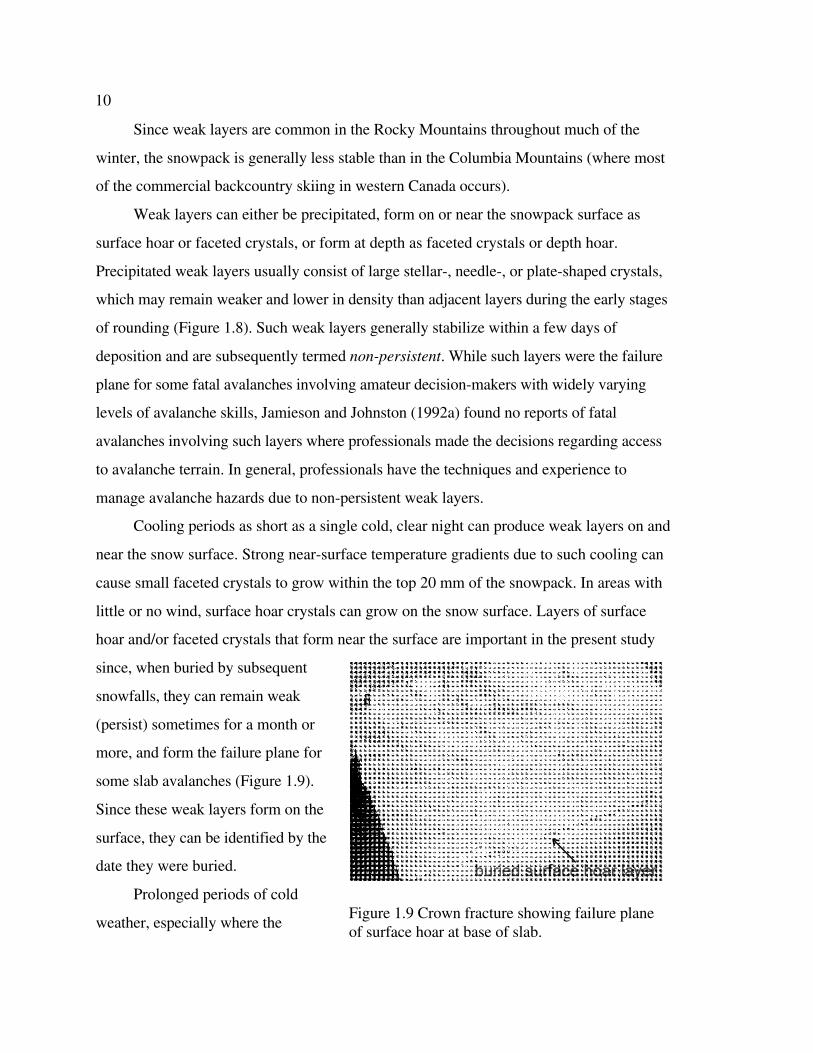


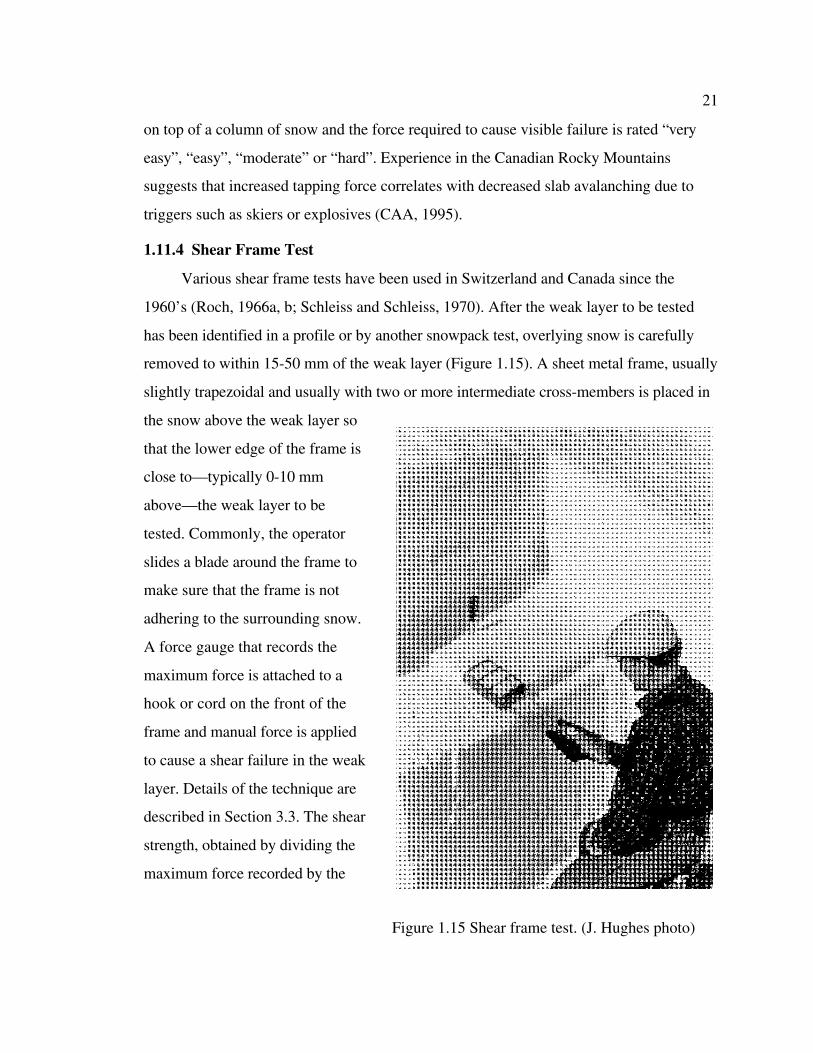


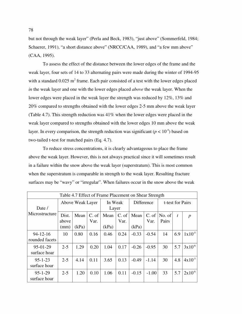


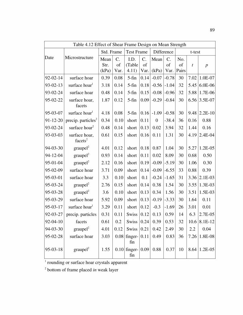


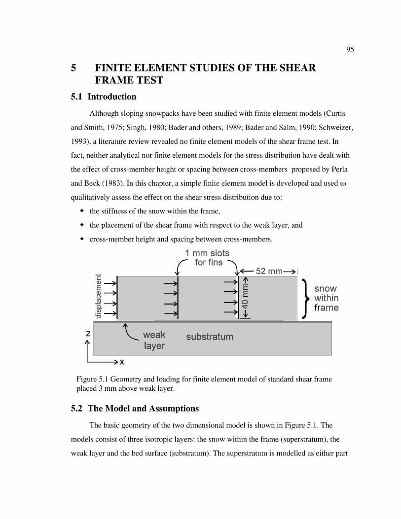


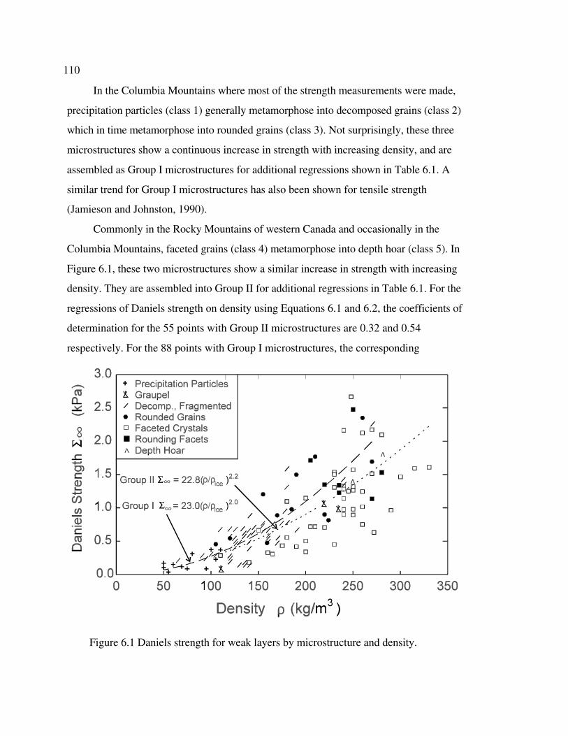


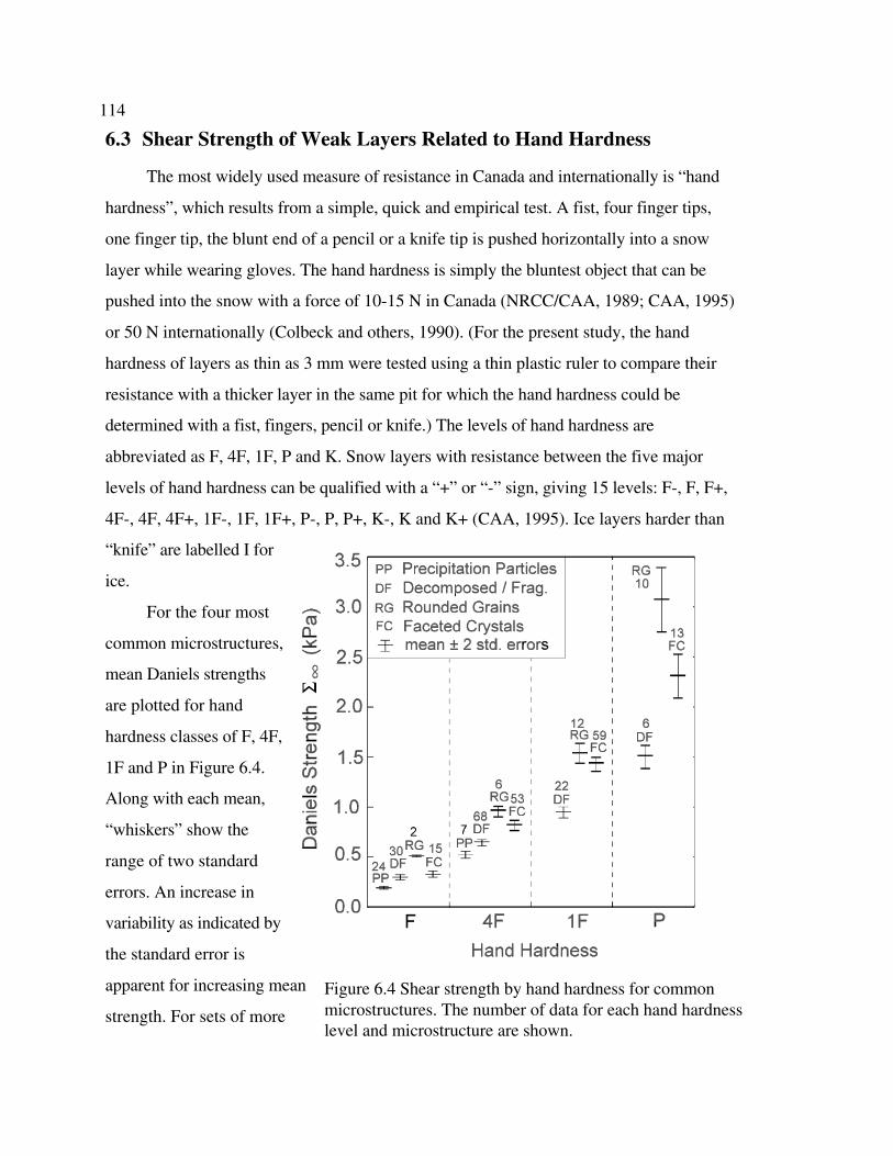


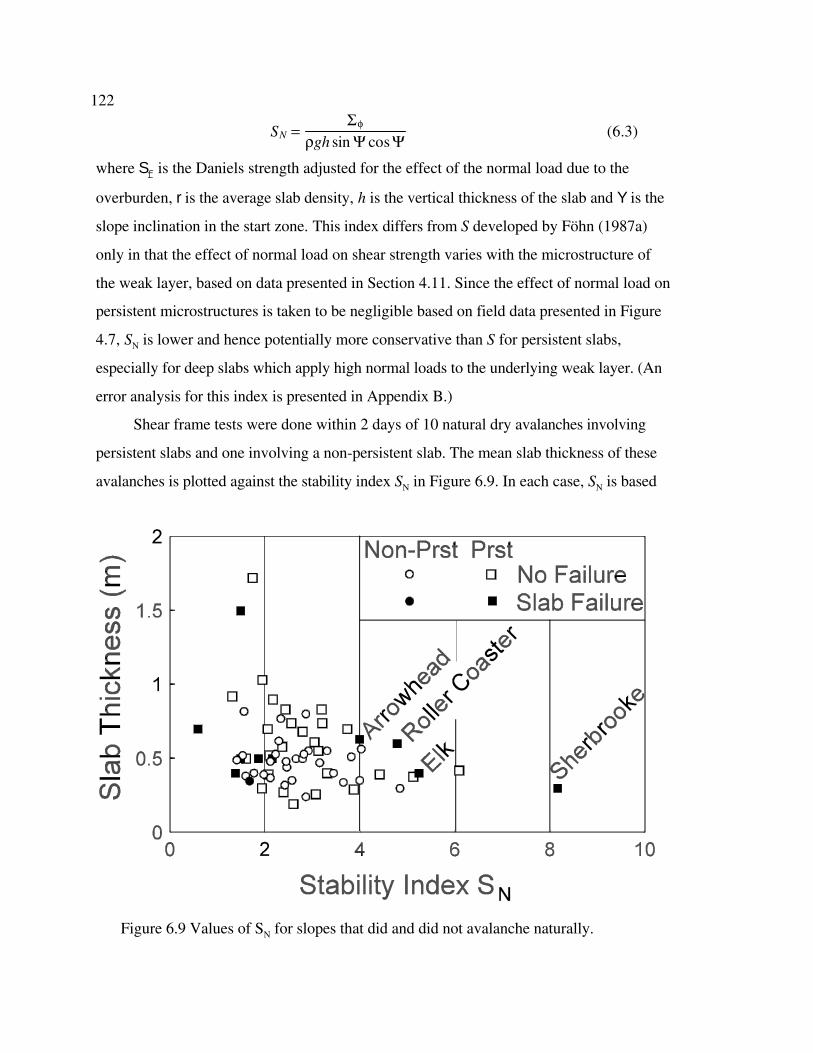


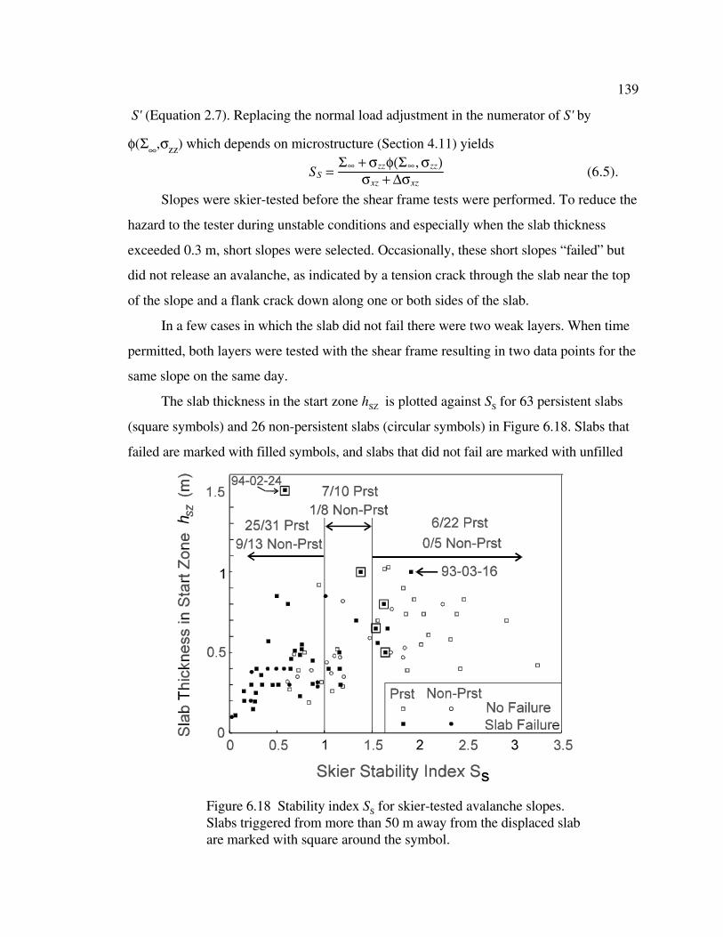


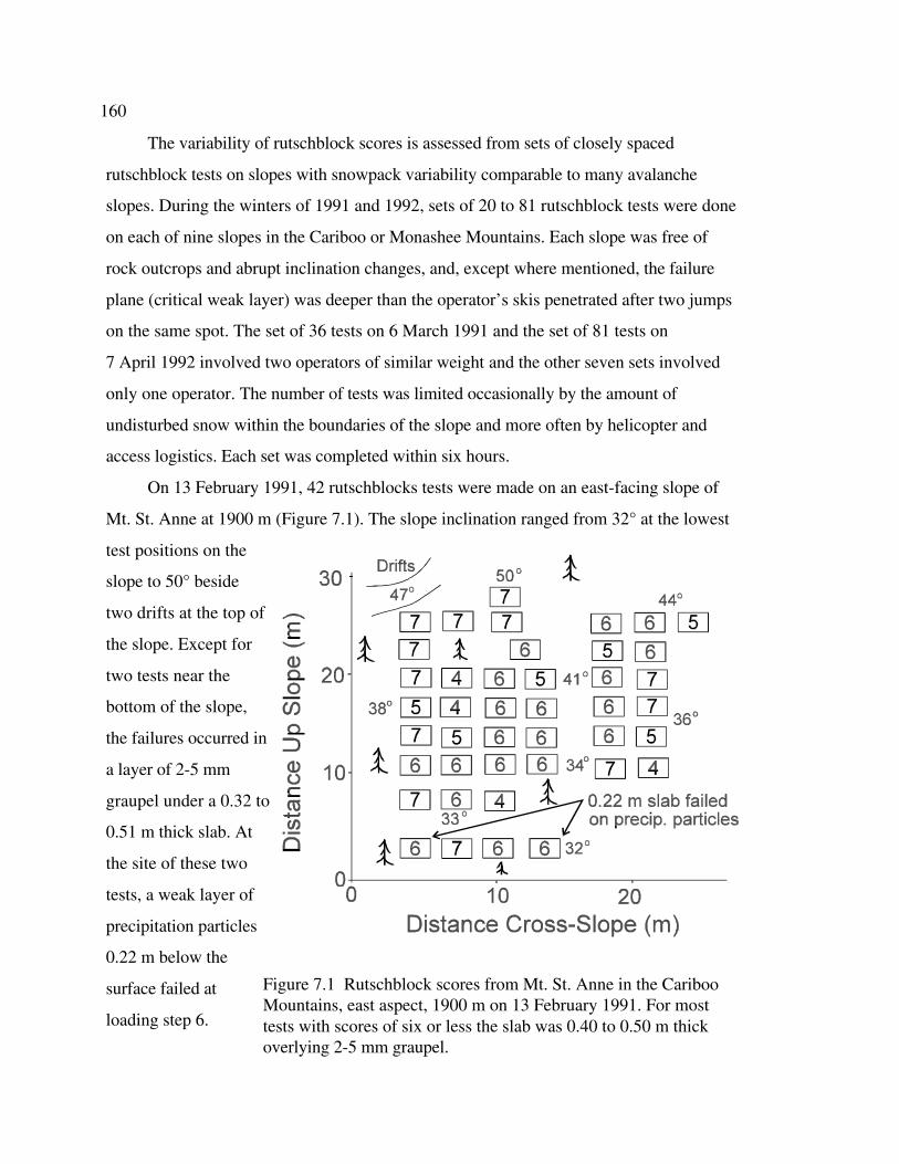


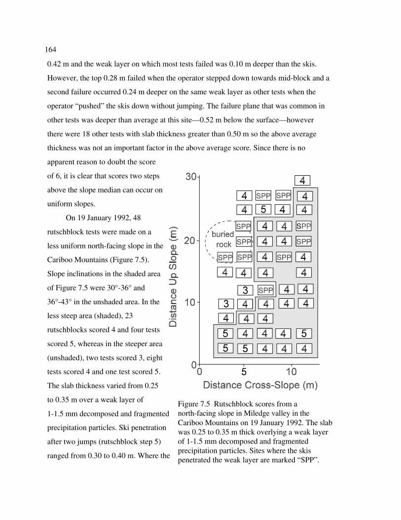

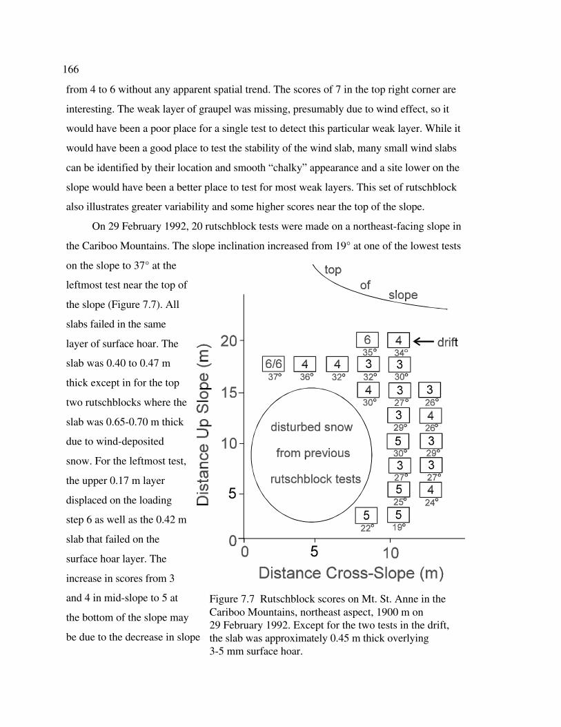


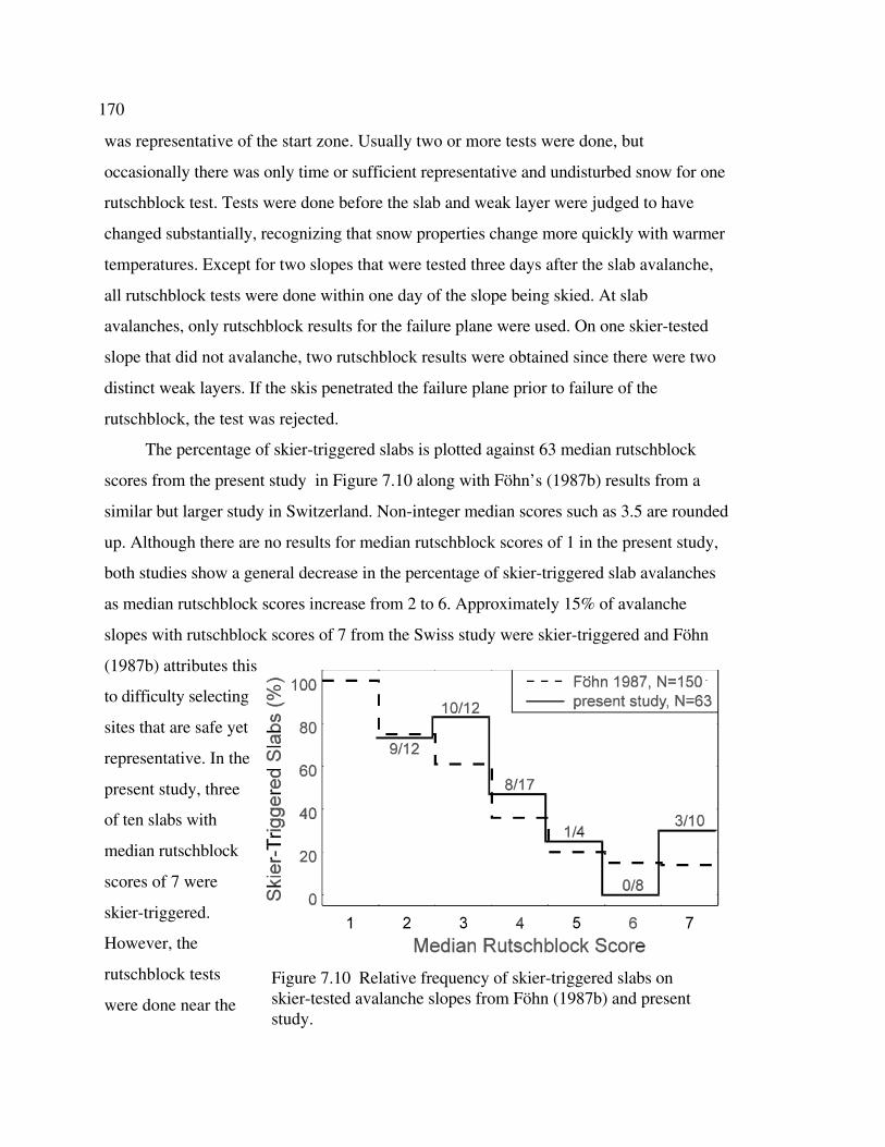


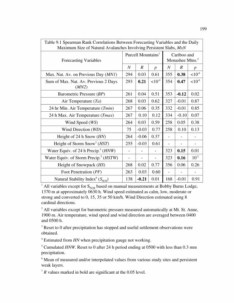


![A model investigation of turbulence-driven pressure ... · sure pumping [Colbeck, 1989] and that pressure pumping by ... suspended from a piece of nylon dental floss, had been in-](https://static.documents.pub/doc/80x56/5b793f757f8b9a7f378d3f23/a-model-investigation-of-turbulence-driven-pressure-sure-pumping-colbeck.jpg)


