Testing diagnostic bioindicators in Prairie streams: Are biological traits and delta

15N of aquatic insects able to detect agricultural impacts?

by

Sophie Nicole Cormier

Bachelor of Science, University of New Brunswick, 2013

A Thesis Submitted in Partial Fulfillment

of the Requirements for the Degree of

Master of Science

in the Graduate Academic Unit of Biology

Supervisor: Joseph M. Culp, Ph.D., Biology

Examining Board: Alexa Alexander-Trusiak, PhD, Biology, Chair

Kerry T.B. MacQuarrie, PhD, Civil Engineering

This thesis is accepted by the

Dean of Graduate Studies

THE UNIVERSITY OF NEW BRUNSWICK

January, 2017

© Sophie Cormier 2017

ii

ABSTRACT

Agricultural activities in the Red River watershed of Manitoba, Canada, can be

significant sources of excess nutrients, sediments and pesticides leading to ecological

effects in streams and downstream Lake Winnipeg. In such multiple stressor

environments, it is difficult to identify, separate and diagnose the cause of

environmental impacts from different agricultural activities using traditional methods

(e.g., taxa assemblage). However, ecological function indicators (e.g., functional feeding

groups) have potential as diagnostic indicators because they lead to the identification of

ecological change pathways. This study evaluated the efficacy of two indicators of

ecological function: biological traits and nitrogen isotopic signatures (δ15N) of benthic

macroinvertebrate. Indicator sensitivity was evaluated by their association with human

activity gradients that define the type and intensity of human activities (i.e., livestock,

wastewater lagoon discharge, crop production). Results indicated that biological traits

and δ15N of BMI were effective diagnostic bioindicators for small scale impacts (e.g.,

riparian condition) and point sources of stressors (e.g., wastewater discharge). However,

catchment scale agricultural activities were not associated with the bioindicators likely

because of hydrological factors affecting the timing of stressor transportation in these

prairie catchments. This study also demonstrated the importance of testing pathways of

human impacts based on conceptual models including the type and magnitude of

exposure to human activities and natural gradients.

iii

DEDICATION

To the little being that experienced this process from within.

iv

ACKNOWLEDGEMENTS

Completing this thesis would not have been possible without the help and advice

of many. First, I would like to thank my supervisor, Joseph Culp, for his wisdom,

patience, and his understanding that life gets in the way. Thank you to my committee

members who also provided invaluable support throughout this process: Wendy Monk,

and Patricia Chambers. I would also like to thank Adam Yates and Bob Brua for their

guidance, especially with the study design, and I am grateful for contributions from

Armin Namayandeh and Edward Krynak towards the development of the trait database.

I was lucky to have great technical assistance from colleagues at the Canadian

Rivers Institute, Environment Canada and the Yates lab. A special thank you goes to

Eric Luiker, Dave Hryn and Courtney Thompson for enduring field work in muddy

Manitoban streams with me. I am also thankful for logistical and technical support from

Kim Rattan and Zoey Duggan. In addition, I want to acknowledge the last minute field

assistance from Alistair Brown, Jacqueline Freeman, Alexandra Loeppky, Jezuele

Milanez, Matt Remple and Doug Watkinson. I would also like to thank Melanie

Deschènes, Kristie Heard, Craig Logan, Kirk Roach, and the SINLAB team for their

help with sample processing, as well as Linley Jesson, Alexa Alexander, Jennifer Lento,

Chris Tyrell, and Bruce Webb for taking the time to answer my questions and offer

advice.

Last but not least, I extend my gratitude to my family and close colleagues for

their encouragement and open ears, especially my parents, Katherine, Brianna,

Stephanie and Aleatha. I also thank my husband for his support, patience and

understanding.

v

Table of Contents

ABSTRACT ..................................................................................................................... ii

DEDICATION ................................................................................................................ iii

ACKNOWLEDGEMENTS ........................................................................................... iv

Table of Contents .............................................................................................................v

List of Tables ................................................................................................................ viii

List of Figures ...................................................................................................................x

1.0 General introduction ..................................................................................................1

1.1 Background ............................................................................................................. 1

1.2 Diagnostic bioindicators.......................................................................................... 4

1.2.1 Structural vs. functional bioindicators ............................................................. 4

1.2.2 Functional bioindicators: biological traits and δ15N ........................................ 5

1.2.3 Testing bioindicators ........................................................................................ 7

1.3 Objectives ................................................................................................................ 8

1.4 Research significance ............................................................................................ 11

1.5 References ............................................................................................................. 12

2.0 Effects of agriculture on stream benthic macroinvertebrate community and

trait composition in Prairie streams .............................................................................19

2.1 Introduction ........................................................................................................... 19

vi

2.2 Methods ................................................................................................................. 24

2.2.1 Study area ....................................................................................................... 24

2.2.2 BMI collection and trait assignment .............................................................. 25

2.2.3 Natural factors and HAGs .............................................................................. 27

2.2.4 Data analysis .................................................................................................. 29

2.3 Results ................................................................................................................... 31

2.3.1 Macroinvertebrate and trait assemblage structure.......................................... 31

2.3.2 Association with environmental variables ..................................................... 33

2.4 Discussion ............................................................................................................. 36

2.4.1 Drivers of trait and taxa beta diversity ........................................................... 36

2.4.2 Biological traits as bioindicators for the RRV ............................................... 40

2.4.3 Conclusions .................................................................................................... 42

2.5 References ............................................................................................................. 43

3.0 Δ15N as a tracer of anthropogenic nitrogen sources in Landscapes of Southern

Manitoba, Canada. .........................................................................................................70

3.1 Introduction ........................................................................................................... 70

3.2 Methods ................................................................................................................. 74

3.21 Study area and experimental design ................................................................ 74

3.22 Data analysis ................................................................................................... 76

3.3 Results ................................................................................................................... 78

vii

3.4 Discussion ............................................................................................................. 79

3.4.1 Response of δ15N to point and non-point sources of nitrogen ....................... 79

3.4.2 δ15N of BMI and POM as bioindicator in the RRV ....................................... 83

3.4.3 Conclusion ..................................................................................................... 84

3.5 References ............................................................................................................. 85

4.0 General conclusion .................................................................................................101

4.1 Stated objectives.................................................................................................. 101

4.2 Drivers of trait and taxa beta diversity ................................................................ 101

4.3 Response of δ15N of BMIs to anthropogenic nitrogen ........................................ 103

4.4 Research implications ......................................................................................... 104

4.5 Conclusions and recommendations ..................................................................... 106

4.6 References ........................................................................................................... 110

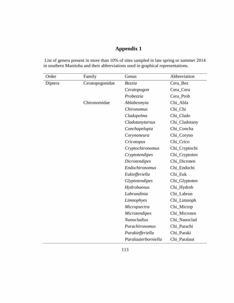
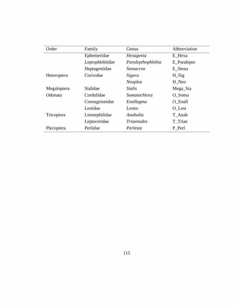
Appendix 1 ....................................................................................................................113

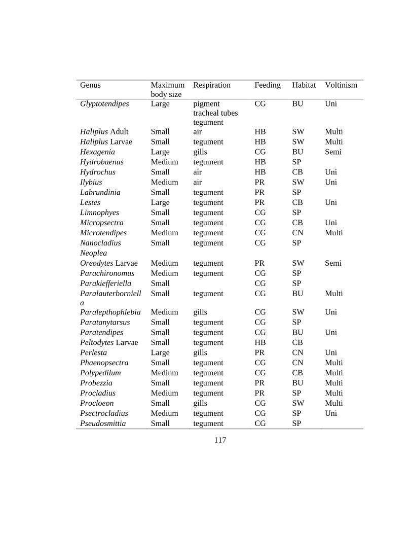
Appendix 2 ....................................................................................................................116

Appendix 3 ....................................................................................................................119

Appendix 4 ....................................................................................................................120

Curriculum Vitae

viii

List of Tables

Table 2.1: Name and catchment description of 20 sites sampled in the Red River Valley

in southern Manitoba, Canada. .................................................................. 51

Table 2.2: Trait categories and trait states included in trait analyses of benthic

macroinvertebrate genera in southern Manitoba and their abbreviations (based on

Poff et al. 2006). ........................................................................................ 52

Table 2.3: Site and reach scale variables sampled in late spring (sp) or summer (su) 2014

for sites in the Red River Valley, southern Manitoba, Canada. Variables not used

in analyses were considered redundant based on Pearson correlation with other

variables of the same scale. ........................................................................ 53

Table 2.4: Catchment scale human activity included in each Principal Component

Analysis (PCA) to determine Human Activity Gradients in southern Manitoba,

Canada. High correlation was determined by a correlation coefficient higher than

0.8. .............................................................................................................. 54

Table 2.5: Distribution (% frequency of occurrence among 20 catchments) and

descriptive statistics of human activity in study catchments of the Red River

Valley, in southern Manitoba, Canada. ...................................................... 55

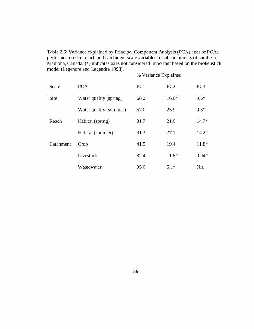
Table 2.6: Variance explained by Principal Component Analysis (PCA) axes of PCAs

performed on site, reach and catchment scale variables in subcatchments of

southern Manioba, Canada. (*) indicates axes not considered important based on

the brokenstick model (Legendre and Legendre 1998). ............................. 56

Table 2.7: Variance explained by axes (PC) of Principal Component Analyses of taxa or

trait assemblages sampled in spring or summer in southern Manitoba, Canada.

.................................................................................................................... 57

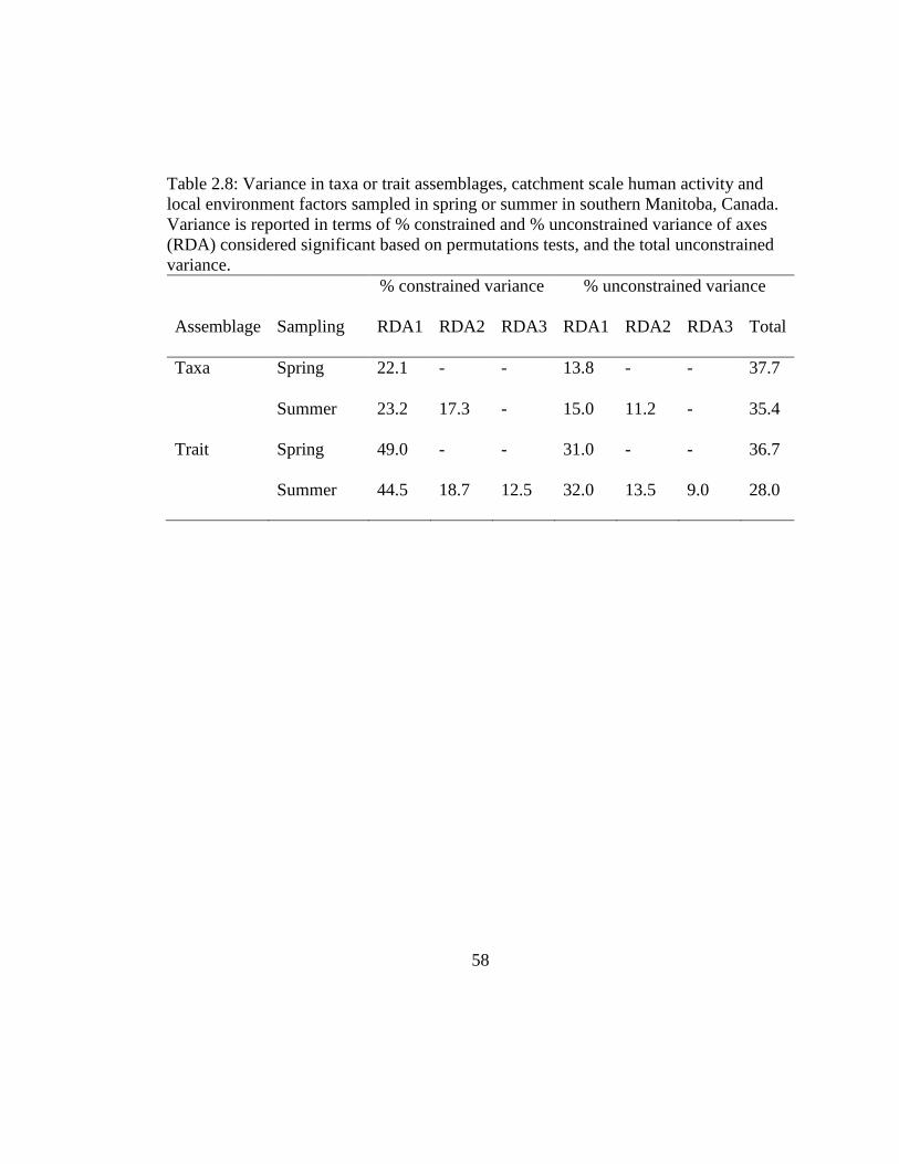
Table 2.8: Variance in taxa or trait assemblages, catchment scale human activity and

local environment factors sampled in spring or summer in southern Manitoba,

Canada. Variance is reported in terms of % constrained and % unconstrained

variance of axes (RDA) considered significant based on permutations tests, and

the total unconstrained variance. ................................................................ 58

Table 3.1: A priori hypotheses of how δ15N of particulate organic matter and primary

consumers may be affected by human activity gradients in subcatchments of the

Red River Valley of southern Manitoba, Canada. The ordinate intercept is

identified by (I). The PCA axes used as predictors are coded using “crop” (crop

types), “live” (type of livestock densities) and “wwt” (wastewater) with PC1

indicating the first axis or PC2, the second axis. ....................................... 90

ix

Table 3.2: Descriptive statistics of δ15N values (‰) for particulate organic matter and

primary consumers sampled during both spring and summer in streams of

southern Manitoba, Canada. ....................................................................... 91

Table 3.3: Comparison of a priori tested models for predicting δ15N changes in primary

consumer taxa sampled in late spring for subcatchments in southern Manitoba,

Canada, using corrected Akaike Information Criterion (AICc). ................ 92

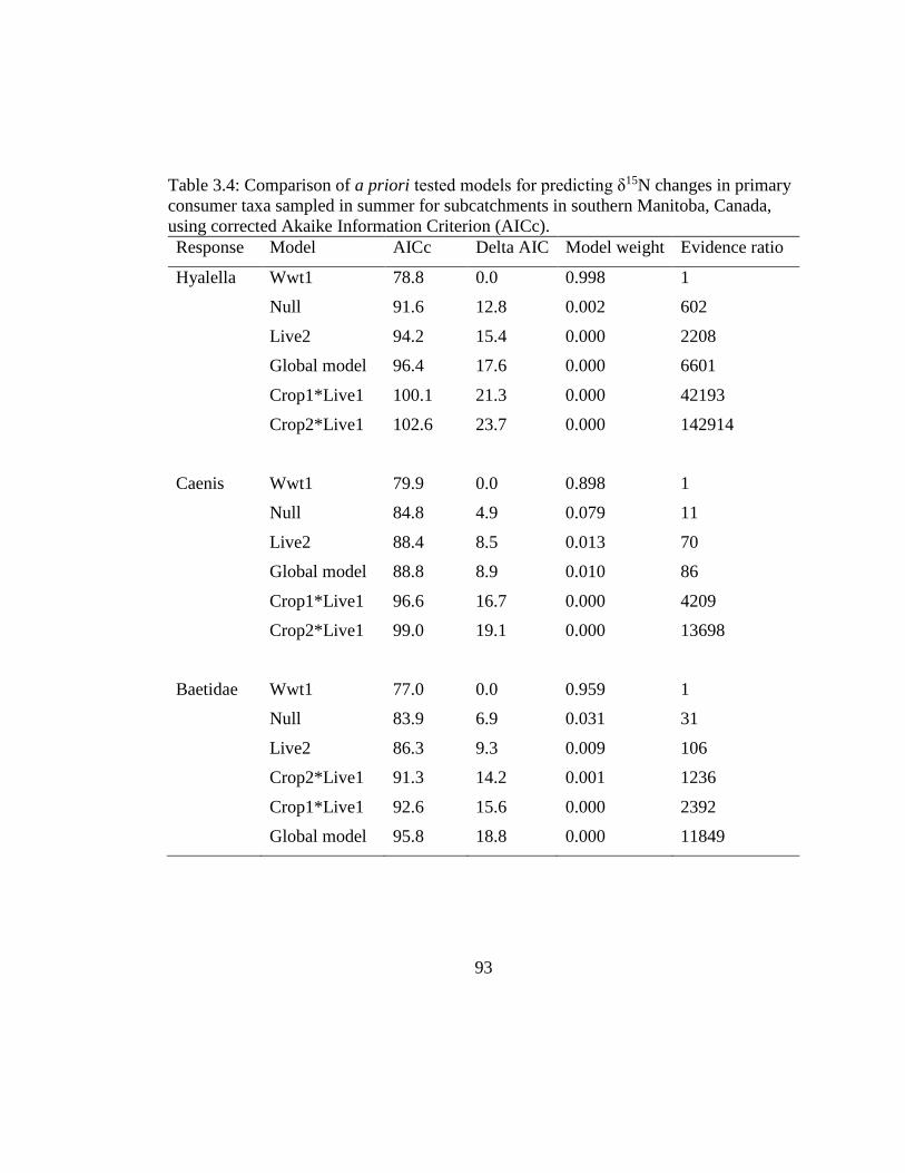
Table 3.4: Comparison of a priori tested models for predicting δ15N changes in primary

consumer taxa sampled in summer for subcatchments in southern Manitoba,

Canada, using corrected Akaike Information Criterion (AICc). ................ 93

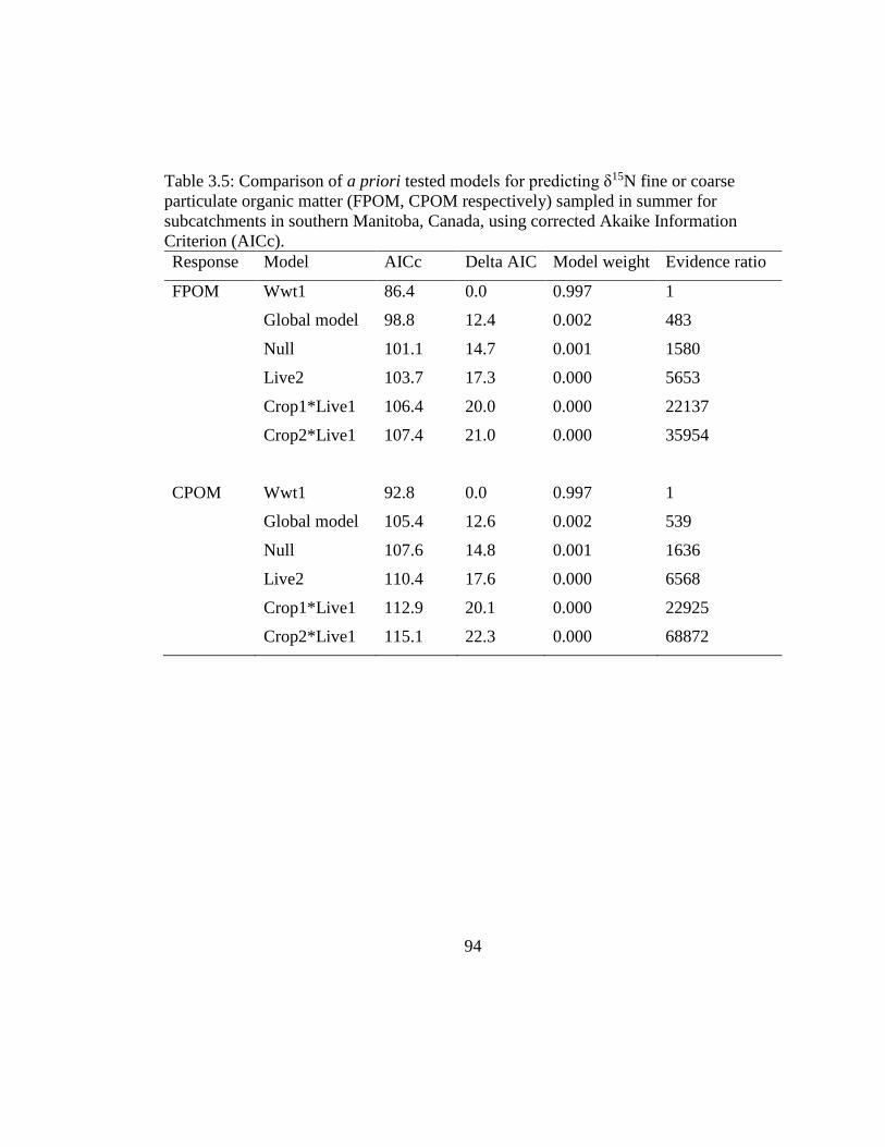
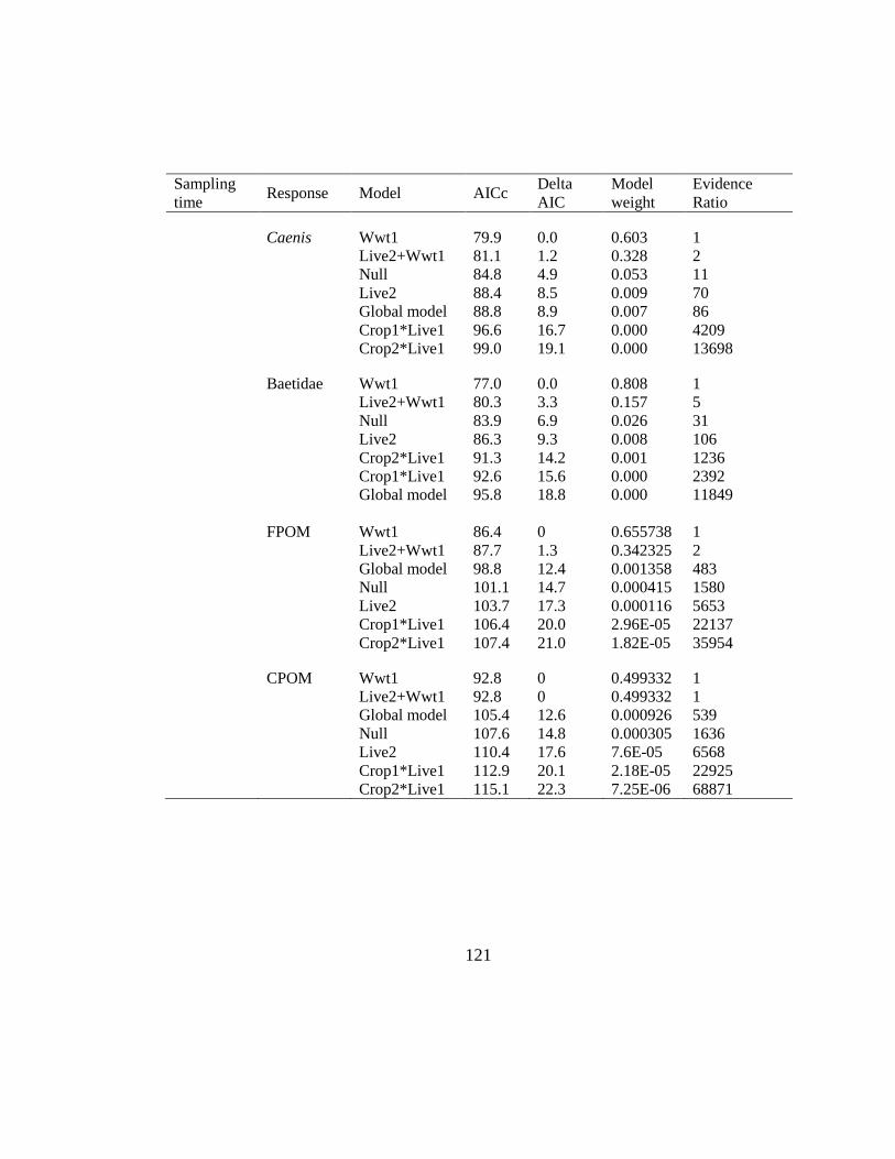
Table 3.5: Comparison of a priori tested models for predicting δ15N fine or coarse

particulate organic matter (FPOM, CPOM respectively) sampled in summer for

subcatchments in southern Manitoba, Canada, using corrected Akaike

Information Criterion (AICc). .................................................................... 94

x

List of Figures

Figure 2.1: Conceptual diagram of broad mechanistic links between catchment scale

human activities, reach scale habitat, site scale water quality and trait categories

in freshwater streams.................................................................................. 59

Figure 2.2: Location of 20 sites and their subcatchments in southern Manitoba, Canada,

sampled in this study. Gray lines represent elevation contours. (Layers were

extracted from Geogratis.ca). ..................................................................... 60

Figure 2.3: Principal Component Analysis (PCA) of the type and intensity of a) crops,

b) livestock, and c) wastewater lagoons for 20 subcatchments in southern

Manitoba, Canada. Abbreviations are listed in Table 2.4. ......................... 61

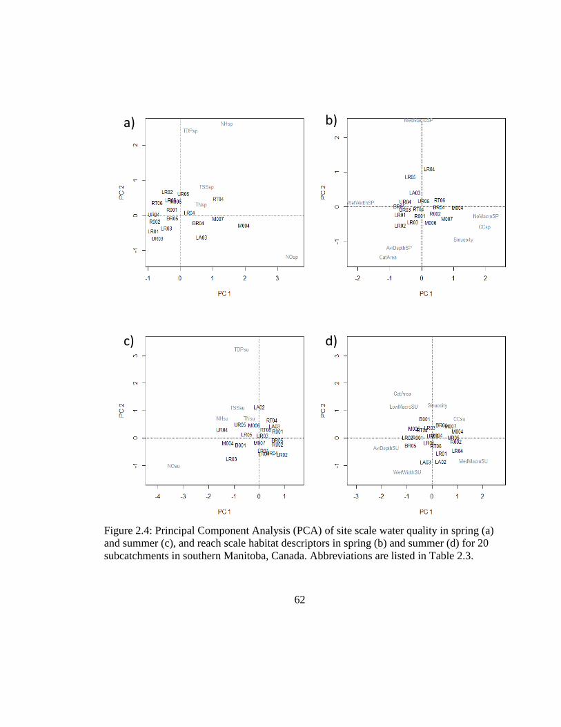
Figure 2.4: Principal Component Analysis (PCA) of site scale water quality in spring (a)

and summer (c), and reach scale habitat descriptors in spring (b) and summer (d)

for 20 subcatchments in southern Manitoba, Canada. Abbreviations are listed in

Table 2.3. .................................................................................................... 62

Figure 2.5: Principal Component Analyses (PCA) of taxa assemblage in spring (a) and

summer (b) (closed circles) measured at 18 (spring) or 20 (summer) study sites

(open circles) in southern Manitoba in 2014. Taxa abbreviation are listed in

Appendix 1. Taxa were labeled by order of importance to limit label overlaps.

.................................................................................................................... 63

Figure 2.6: Principal Component Analyses (PCA) of trait assemblage in spring (a) and

summer (b) summer assemblage (closed circles) sampled at 18 (spring) or 20

(summer) study sites (open circles) in southern Manitoba in 2014. Trait

abbreviation are listed in Table 2.2. ........................................................... 64

Figure 2.7: Redundancy Analysis (RDA) of presence-absence of aquatic insect genera

sampled in late spring 2014 in 18 sites of southern Manitoba, Canada. Taxa

abbreviations are listed in Appendix 1. ...................................................... 65

Figure 2.8: Redundancy Analysis (RDA) of presence-absence of aquatic insect genera

sampled in summer 2014 in 20 sites of southern Manitoba, Canada. Taxa

abbreviations are listed in Appendix 1. ...................................................... 66

Figure 2.9: Redundancy Analysis (RDA) of presence-absence of aquatic insect’ traits

sampled in late spring 2014 in 18 sites of southern Manitoba, Canada. Trait

abbreviations are listed in Table 2.2. ......................................................... 67

xi

Figure 2.10: Redundancy Analysis (RDA) of presence-absence of aquatic insect’ traits

sampled in summer 2014 in 20 sites of southern Manitoba, Canada. Trait

abbreviations are listed in Table 2.2. ......................................................... 68

Figure 2.11: Redundancy Analysis (showing RDA2 and RDA3) of presence-absence of

aquatic insect’ traits sampled in summer 2014 in 20 sites of southern Manitoba,

Canada. Trait abbreviations are listed in Table 2.2. ................................... 69

Figure 3.1: Conceptual model of δ15N changes from landscape nitrogen sources to the

food web. (+) indicates an enrichment in δ15N, while (-) indicates a depletion.

Because the influence of both crops is dependent upon whether livestock manure

or synthetic fertilizer is the dominant source of nitrogen applied on the fields, the

relationship between crops and δ15N of the food web is difficult to predict. This

uncertainty is denoted by (?). ..................................................................... 95

Figure 3.2: Mean δ15N (± 1SD) of primary consumers and particulate organic matter

sampled during spring and summer 2014 in streams of southern Manitoba,

Canada. ....................................................................................................... 96

Figure 3.3: Relationship between the δ15N of all BMI and the wastewater HAG

(wwtPC1) sampled in spring or summer in subcatchments of southern Manitoba,

Canada. ....................................................................................................... 97

Figure 3.4: Relationship between the δ15N of particulate organic matter (fine, FPOM;

coarse, CPOM) and the wastewater HAG (wwtPC1) sampled in spring or

summer in subcatchments of southern Manitoba, Canada. ........................ 98

Figure 3.5: Conditional plots of δ15N of Hyalella in spring and (a) beef cattle production

(livePC2) while controlling for wwtPC1, or (b) wastewater HAG (wwtPC1)

while controlling for livePC2. Shaded areas represent confidence bands

(Breheny and Burchett 2013). .................................................................... 99

Figure 3.6: Conditional plot of δ15N of Coarse Particulate Organic Matter (CPOM) and

beef cattle production (livePC2) while controlling for wwtPC1 with (a) and

without (b) UR05. Shaded areas represent confidence bands (Breheny and

Burchett 2013). ......................................................................................... 100

1

1.0 General introduction

1.1 Background

Agricultural land use alters the natural landscapes of watersheds and causes the

degradation of stream ecosystem health (Moss 2008). The major environmental stressors

associated with agriculture are excess nutrients, fine sediment and pesticides (Allan

2004), all of which can affect aquatic ecosystems directly (e.g., pesticide-related

mortality, Shulz and Liess 1999) and indirectly (e.g., altered herbivory rates; Delong and

Brusven 1998). Synthetic fertilizer applied on crops and manure from livestock

production causes increased nutrient inputs to streams through runoff (Carpenter et al.

1998, Chambers et al. 2009). This excess nutrient input can affect aquatic productivity

causing bottom-up effects through the food web, such as a change in invertebrate

density (Correll 1998, Rabalais 2002). Sediment inputs from tillage (Lobb et al. 2007),

livestock trampling (Kyriakeas and Watzin 2006) and clearing of riparian vegetation

(Meador and Goldstein 2003) can also have significant deleterious effects on stream

communities. For example, fine sediments may interfere with respiration or feeding

mechanisms (e.g., gills), reduce food source availability through smothering or light

reduction, and decrease the quality of benthic habitats (Wood and Armitage 1997,

Henley et al. 2000). Such impacts are difficult to quantify because of possible

2

interactions among stressors (Townsend et al. 2008, Matthaei et al. 2010, Magbanua et

al. 2013), and are difficult to attribute to specific agricultural practices in large

watersheds because several types of crops and livestock production co-occur within the

landscape creating multiple stressor environments (Allan 2004).

The Red River Valley (RRV) in southern Manitoba, Canada, is an area with

intensive agriculture and, thus, a multiple stressor environment (Yates et al. 2012). This

watershed drains into Lake Winnipeg, the 10th largest lake in the world, and is the main

contributor of nutrients to the lake leading to increased algal blooms and related

ecosystem shifts (Jones and Armstrong 2001, Bunting et al. 2011, Schindler et al.

2012). The hyper-eutrophic state of Lake Winnipeg has serious repercussions for the

fisheries and tourism industries of the area (Environment Canada and Manitoba Water

Stewardship 2011) and has led to intensive research and monitoring to describe these

ecosystem changes in the hopes of developing appropriate mitigation measures

(Wassenaar and Rao 2012). As the stressors that affect the lake, most notably excess

nutrients, arise from land based activities in the RRV, managing these human activities

in the upstream watershed will be critical to address environmental changes in the lake

(Dodds and Oaks 2008, Schindler et al. 2012). An important step that still remains for

successful monitoring and mitigation of impacts is the development of monitoring tools

capable of diagnosing stressor-specific impacts to understand how to effectively manage

3

each of these, and to test the effectiveness of management actions (Yates et al. 2012,

2014).

Indicators based on biota (i.e., bioindicators) have been widely used to describe

changes in the general health of ecosystems, but there is a need for developing

diagnostic bioindicators to better serve management and monitoring efforts (Downes

2010, Rapport and Hilden 2013). Bioindicators can integrate effects over longer

timeframes and have advantages over point samples of water quality (Cairns et al.

1993). A common group of organisms used as bioindicators are benthic

macroinvertebrates (BMI; Bonada et al. 2006). These organisms characterize the effects

of local environmental conditions because of their relatively limited dispersal and short

generation time (Cairns et al. 1993). Furthermore, BMI may be appropriate as

diagnostic indicators because they have diverse ecological roles (Wallace and Webster

1996) and stressor tolerance (Bonada et al. 2006), and thus may be useful in a multiple

stressor watershed such as the RRV. Therefore, the aim of this thesis is to use BMI to

develop diagnostic indicators relevant to agricultural activities in the RRV.

4

1.2 Diagnostic bioindicators

1.2.1 Structural vs. functional bioindicators

Reliable diagnostic bioindicators need to detect specific stressor-effect

relationships based on a priori mechanistic hypotheses (Dale and Bayeler 2001, Bonada

et al. 2006, Downes 2010). Structural indicators, such as taxa metrics summarizing BMI

communities, have been extensively used to identify general degradation of stream

health related to human activities (Karr 1991, Cairns et al. 1993, Allan 2004). For

example, communities exposed to agricultural pollutants commonly experience a loss of

intolerant taxa resulting in decreased taxa evenness (Delong and Brusven 1998, Friberg

et al. 2003, Sutherland et al. 2012). However, it can be difficult to infer causation with

structural bioindicators in multiple stressor environments because they often respond in

a similar way to a wide range of environmental stressors (Dolédec et al. 2006, Palmer

and Febria 2012) and may include noise arising from biotic factors such as recruitment

and dispersal (Bunn and Davies 2000).

Indicators of ecological function describe ecosystem processes, such as nutrient

cycling (Dale and Beyeler 2001), and are considered to have greater diagnostic power

than structural indicators because they are more directly linked to pathways of

ecological change (Palmer and Febria 2012). Furthermore, because simple but powerful

predictions about specific processes can be tested using functional indicators, it is

5

possible to infer causal relationships and better isolate the effects of independent

stressors (Bunn and Davies 2000, Culp et al. 2010). Thus, it is not surprising that

functional indicators commonly demonstrate a stronger response to stressor gradients

than structural indicators (Sandin and Solimini 2009). Functional indicators may also be

better suited for studying impacts in large watersheds because they provide more

consistent relationships to human impacts over large spatial scales (Bêche et al. 2006,

Pollard and Yuan 2010, Dolédec et al. 2011). Two functional bioindicators are

considered in this thesis based on recommendations by Yates et al. (2012, 2014),

namely biological traits and the nitrogen isotopic signature of BMI (δ15N).

1.2.2 Functional bioindicators: biological traits and δ15N

Biological traits include characteristics of organisms associated with adaptations

to their environment (e.g., functional feeding groups, maximum body size, respiration,

locomotion). Traits have the potential to be good diagnostic bioindicators in multiple

stressor environments because their relationship with pathways of environmental change

are predictable (Poff 1997) and they often respond independently to different stressors

(Townsend and Hildrew 1994, Poff 1997, Culp et al. 2010, Statzner and Bêche 2010).

For example, Lange et al. (2014) found that life-history traits (e.g., life duration of

adults) of BMI in New Zealand streams were associated with farming intensity, while

feeding habitats and respiration traits were indicative of water abstraction. Although this

6

approach does not consider variation of traits within individual organisms (e.g.,

maximum body size of taxa based on the literature vs. average body size of individuals

collected), aggregating species to create biological trait categories simplifies the study of

multi-species assemblages (Poff 1997) while retaining more information than composite

indexes (Statzner and Bêche 2010). In addition, by only including traits that can be

mechanistically linked to the stressor of interest, it is possible to avoid confounding

interpretation from traits that are evolutionary linked while strengthening the ability to

discriminate stressors (Poff et al. 2006, Statzner and Bêche 2010).

In addition to biological traits, the δ15N signature of BMI, a stable isotope

approach, is a promising diagnostic bioindicator because it may allow identification of

independent sources of anthropogenic nitrogen (Anderson and Cabana 2005, Niemi et

al. 2011, Winemiller et al. 2011, Clapcott et al. 2012). Human activities produce

nitrogen with different δ15N signatures. For example, synthetic fertilizers often have low

nitrogen isotopic values compared to manure or wastewater (Bedard-Haughn et al.

2003). When these nitrogen inputs with relatively unique δ15N signatures reach the

aquatic environment and are assimilated within the food web, they change the

proportion of heavy to light nitrogen isotopes in tissues of primary producers and

consumers in a predictable manner (Peterson and Fry 1987). Moreover, because the

δ15N signature of BMI integrates temporal variation in exposure to excess nitrogen, it

7

may help infer the source in addition to the magnitude of nitrogen assimilation from

human sources in the food chain (Bedard-Haughn et al. 2003).

1.2.3 Testing bioindicators

Because bioindicators can be affected by natural factors in addition to human

impacts, the effectiveness of the proposed bioindicators must be tested in the RRV prior

to implementing them in monitoring programs. For example, natural variation unrelated

to human activities, such as catchment geology, may affect traits independently and

confound conclusions about human impacts (Poff 1997, Yates and Bailey 2010, Heino

et al. 2013). In addition, local factors relating to nitrogen transformation and cycling

affect the natural δ15N baseline and the δ15N of anthropogenic sources, thus

necessitating local testing and validation to ensure the effectiveness of this tool in

identifying specific nitrogen sources (Bedard-Haughn et al. 2003, Diebel and Vander

Zanden 2009). Interpreting changes in biological traits or δ15N signature of BMI based

on associations from other geographical regions may result in falsely attributing

differences to human impacts.

A key characteristic of a successful diagnostic bioindicator is that it exhibits a

known and consistent response to specific anthropogenic stressors (Dale and Beyeler

2001, Bonada et al. 2007). Thus, a multiple catchment design has been proposed as a

powerful approach for testing the effectiveness of bioindicators over gradients of

8

exposure to human activities (Yates and Bailey 2007). Bailey et al. (2007) proposed the

use of conceptual models, representing the pathways of effects in response to specific

human land use, to enable inferences of causal relationships between bioindicators and

human activities. Quantifying exposure to human activities has often involved using

coarse descriptions of land use (e.g., % agricultural land cover; Allan 2004), but these

may not be appropriate for diagnostic studies in catchments with intensive agriculture

because catchments with a similar extent of agriculture may differ in specific

agricultural practices, the connectivity of agricultural land with the stream, and the

consequent ecological effects (e.g., unequal contribution of nutrients from different crop

types; Yates and Bailey 2010). Instead, Human Activity Gradients (HAGs) that quantify

the type and magnitude of specific human activities (e.g., types of crops such as small

grain production) have been shown to be an effective and comprehensive measure of

exposure to anthropogenic stressors in multiple stressor watersheds (Yates et al. 2012).

Natural gradients can be included to support hypotheses about the pathway of effects of

human impacts (Bailey et al. 2007) and to identify possible covariation between human

impacts and unrelated natural variation (Yates and Bailey 2006).

1.3 Objectives

This thesis aims to determine the utility of two bioindicators based on BMI

assemblages (i.e., biological traits and δ15N signatures) to diagnose human impacts in

9

the agricultural watershed of the RRV by testing their response along HAGs as

described by Yates et al. (2012). Previous work in southern Manitoba revealed that the

δ15N signature of BMI may be a good diagnostic bioindicator for the region because of

relationships between some human activities and primary producers (Yates et al. 2014).

However, the potential of biological traits of BMI to be used as diagnostic bioindicators

has not been tested in the RRV.

The first objective, examined in Chapter 2, compared the sensitivity of biological

traits and community structure of BMI to specific human activities with the goal of

determining if traits have better diagnostic power than the structural approach, as

predicted by the literature. It is expected that a trait-based approach is more sensitive to

stressors of interest because of a mechanistic linkage with pathways of interest, greater

seasonal stability and consistency across broad spatial scales when compared to a

taxonomic approach (Culp et al. 2010). The trait-based approach included the

formulation of a priori mechanistic hypotheses based on a conceptual diagram

describing predicted relationships among human activities, local habitat and biological

traits (Figure 2.1). It was predicted that: (1) high exposure to pesticides favors traits that

promote resilience to stress, more specifically smaller body size and short generation

time (Townsend and Hildrew 1994, Liess et al. 2005); (2) excess nutrients increases

herbivores, shredders and/or collector-filterers if accompanied with higher food

10

availability and less tegument respiration if the effect decreases dissolved oxygen

concentrations (Compin and Céréghino 2007, Carlisle and Hawkins 2008, Feio and

Dolédéc 2012); and (3) excess fine sediment decreases the occurrence of traits such as

aquatic respiration, filter feeding, scraping and shredding because of the interference

from sediment particles or reduction in food source availability, coupled with an

increase in burrowers which prefer fine sediment bottoms (Rabeni et al. 2005,

Magbanua et al. 2013).

The second objective, explored in Chapter 3, determined whether the δ15N

signature of BMI in the RRV could be used to identify sources of anthropogenic

nitrogen in streams of the RRV. Primary consumers were chosen as the food web

component to evaluate δ15N as a potential tracer of nitrogen sources in order to limit the

influence of fractionation due to trophic position within a food web (Peterson and Fry

1987). In addition, the δ15N signature of particulate organic matter (POM) was included

to represent the base of the food web. A conceptual model describing the predicted

influence of different anthropogenic nitrogen sources on the baseline δ15N assimilated in

the food web was used to develop hypotheses (Figure 3.1). This model is based on

literature observations and predicts that point sources of anthropogenic nitrogen, such as

livestock feedlots and wastewater lagoons, would enrich δ15N of POM and BMI because

both manure and wastewater discharge tend to have high δ15N compared to the natural

11

baseline (Bedard-Haughn et al. 2003, Anderson and Cabana 2006, Diebel and Vander

Vander Zanden 2009). Furthermore, the relationship between cropland and δ15N of BMI

in southern Manitoba was predicted to be dependent on the dominant fertilizer, synthetic

or manure, used in a particular catchment. In contrast to manure that has a high δ15N,

synthetic fertilizers tend to have a low δ15N compared to the natural baseline (Bedard-

Haughn et al. 2003). Because information about the amount and type of fertilizer

applied in catchments of the study area was not available, more specific predictions

about the influence of nitrogen from crop runoff could not be formulated.

1.4 Research significance

Indicator and baseline studies, such as the current thesis research, are an

important step toward understanding the effects of agriculture in prairie ecosystems and

improving diagnostic techniques in multiple stressor watersheds. This thesis will

contribute to research for the Tobacco Creek Model Watershed Research Consortium

funded by the Canadian Water Network in its goal of developing localized monitoring

frameworks that can be used to monitor the efficiency of new regulations and best

management practices. In addition, the study contributes to the Lake Winnipeg Basin

Initiative, led by Environment Canada, by assessing the suitability of nutrient

monitoring using aquatic animals as indicators.

12

The thesis is written in manuscript format and consequently, there is some

redundancy between this section and the introduction of the next two chapters.

1.5 References

Allan J.D. (2004) Landscapes and riverscapes: the influence of land use on stream

ecosystems. Annual Review of Ecology, Evolution, and Systematics 35, 257–284.

Anderson C. & Cabana G. (2005) 15 N in riverine food webs: effects of N inputs from

agricultural watersheds. Canadian Journal of Fisheries and Aquatic Sciences 340,

333–340.

Anderson C. & Cabana G. (2006) Does delta 15N in river food webs reflect the intensity

and origin of N loads from the watershed? The Science of the total environment

367, 968–978.

Bailey R.C., Reynoldson T.B., Yates A.G., Bailey J. & Linke S. (2007) Integrating

stream bioassessment and landscape ecology as a tool for land use planning.

Freshwater Biology 52, 908–917.

Bêche L.A., McElravy E.P. & Resh V.H. (2006) Long-term seasonal variation in the

biological traits of benthic-macroinvertebrates in two Mediterranean-climate

streams in California, U.S.A. Freshwater Biology 51, 56–75.

Bedard-Haughn A., van Groenigen J.W. & van Kessel C. (2003) Tracing 15N through

landscapes: potential uses and precautions. Journal of Hydrology 272, 175–190.

Bonada N., Prat N., Resh V.H. & Statzner B. (2006) Developments in aquatic insect

biomonitoring: a comparative analysis of recent approaches. Annual review of

entomology 51, 495–523.

Bonada N., Rieradevall M. & Prat N. (2007) Macroinvertebrate community structure

and biological traits related to flow permanence in a Mediterranean river network.

Hydrobiologia 589, 91–106.

13

Bunn S. & Davies P. (2000) Biological processes in running waters and their

implications for the assessment of ecological integrity. Hydrobiologia 422, 61–70.

Bunting L., Leavitt P., Wissel B., Laird K.R., Cumming B.F., St. Amand A., et al.

(2011) Sudden ecosystem state change in Lake Winnipeg, Canada, caused by

eutrophication arising from crop and livestock production during the 20th century.

Winnipeg, Canada.

Cairns J., McCormick P. V. & Niederlehner B.R. (1993) A proposed framework for

developing indicators of ecosystem health. Hydrobiologia 263, 1–44.

Carlisle D.M. & Hawkins C.P. (2008) Land use and the structure of western US stream

invertebrate assemblages: predictive models and ecological traits. Journal of the

North American Benthological Society 27, 986–999.

Carpenter S.R., Caraco N.F., Correll D.., Howarth R.W., Sharpley A.N. & Smith V.H.

(1998) Nonpoint pollution of surface waters with phosphorus and nitrogen.

Ecological Applications 8, 559–568.

Chambers P.A., M. G., Dixit S.S., Benoy G.A., Brua R.B., Culp J.M., et al. (2009)

Nitrogen and phosphorus standards to protect the ecological condition of

Canadian streams, rivers and coastal waters. National Agri-Environment

Standards Initiative Synthesis Report No. 11. Environment Canada, Gatineau,

Quebec.

Clapcott J.E., Collier K.J., Death R.G., Goodwin E.O., Harding J.S., Kelly D., et al.

(2012) Quantifying relationships between land-use gradients and structural and

functional indicators of stream ecological integrity. Freshwater Biology 57, 74–90.

Compin A. & Céréghino R. (2007) Spatial patterns of macroinvertebrate functional

feeding groups in streams in relation to physical variables and land-cover in

Southwestern France. Landscape Ecology 22, 1215–1225.

Correll D.L. (1998) The role of phosphorus in the eutrophication of receiving waters: a

review. Journal of Environment Quality 27, 261-266.

14

Culp J.M., Armanini D.G., Dunbar M.J., Orlofske J.M., Poff N.L., Pollard A.I., et al.

(2010) Incorporating traits in aquatic biomonitoring to enhance causal diagnosis

and prediction. Integrated environmental assessment and management 7, 187–197.

Dale V.H. & Beyeler S.C. (2001) Challenges in the development and use of ecological

indicators. Ecological Indicators 1, 3–10.

Delong M.D. & Brusven M.A. (1998) Macroinvertebrate community structure along the

longitudinal gradient of an agriculturally impacted stream. Environmental

management 22, 445–457.

Diebel M.W. & Vander Zanden M.J. (2009) Nitrogen stable isotopes in streams: effects

of agricultural sources and transformations. Ecological applications 19, 1127–

1134.

Dodds W.K. & Oakes R.M. (2008) Headwater Influences on Downstream Water

Quality. Environmental Management 41, 367–377.

Dolédec S., Phillips N., Scarsbrook M., Riley R.H. & Townsend C.R. (2006)

Comparison of structural and functional approaches to determining landuse effects

on grassland stream invertebrate communities. Journal of the North American

Benthological Society 25, 44–60.

Dolédec S., Phillips N. & Townsend C.R. (2011) Invertebrate community responses to

land use at a broad spatial scale: trait and taxonomic measures compared in New

Zealand rivers. Freshwater Biology 56, 1670–1688.

Downes B.J. (2010) Back to the future: little-used tools and principles of scientific

inference can help disentangle effects of multiple stressors on freshwater

ecosystems. Freshwater Biology 55, 60–79.

Environment Canada & Manitoba Water Stewardship (2011) State of Lake Winnipeg:

1999 to 2007. Winnipeg, MB.

Feio M.J. & Dolédec S. (2012) Integration of invertebrate traits into predictive models

for indirect assessment of stream functional integrity: A case study in Portugal.

Ecological Indicators 15, 236–247.

15

Friberg N., Lindstrøm M., Kronvang B. & Larsen S.E. (2003)

Macroinvertebrate/sediment relationships along a pesticide gradient in Danish

streams. Hydrobiologia 494, 103–110.

Heino J., Schmera D. & Erős T. (2013) A macroecological perspective of trait patterns

in stream communities. Freshwater Biology 58, 1539–1555.

Henley W.F., Patterson M.A., Neves R.J. & Lemly A.D. (2000) Effects of sedimentation

and turbidity on lotic food webs: a concise review for natural resource managers.

Reviews in Fisheries Science 8, 125–139.

Jones G. & Armstrong N. (2001) Long-term trends in total nitrogen and total

phosphorus concentrations in Manitoba streams. Winnipeg, MB.

Karr J.R. (1991) Biological integrity : a long-neglected aspect of water resource

management. Ecological Applications 1, 66–84.

Kyriakeas S.A. & Watzin M.C. (2006) Effects of adjacent agricultural activities and

watershed characteristics on stream macroinvertebrate communities. Journal of the

American Water Resources Association 42, 425–441.

Liess M. & Von Der Ohe P.C. (2005) Analyzing effects of pesticides on invertebrate

communities in streams. Environmental Toxicology and Chemistry 24, 954.

Lobb D.A., Huffman E. & Reicosky D.C. (2007) Importance of information on tillage

practices in the modelling of environmental processes and in the use of

environmental indicators. Journal of Environmental Management 82, 377–387.

Magbanua F.S., Townsend C.R., Hageman K.J. & Matthaei C.D. (2013) Individual and

combined effects of fine sediment and the herbicide glyphosate on benthic

macroinvertebrates and stream ecosystem function. Freshwater Biology 58, 1729–

1744.

Matthaei C.D., Piggott J.J. & Townsend C.R. (2010) Multiple stressors in agricultural

streams: interactions among sediment addition, nutrient enrichment and water

abstraction. Journal of Applied Ecology 47, 639–649.

16

Meador M.R. & Goldstein R.M. (2003) Assessing water quality at large geographic

scales: Relations among land use, water physicochemistry, riparian condition, and

fish community structure. Environmental Management 31, 504–517.

Moss B. (2008) Water pollution by agriculture. Philosophical transactions of the Royal

Society of London. Series B, Biological sciences 363, 659–666.

Niemi G.J., Reavie E.D., Peterson G.S., Kelly J.R., Johnston C.A., Johnson L.B., et al.

(2011) An integrated approach to assessing multiple stressors for coastal Lake

Superior. Aquatic Ecosystem Health & Management 14, 356–375.

Palmer M.A. & Febria C.M. (2012) Ecology. The heartbeat of ecosystems. Science 336,

1393–1394.

Peterson B.J. & Fry B. (1987) Stable isotopes in ecosystem studies. Annual Review of

Ecology and Systematics 18, 293–320.

Poff N.L. (1997) Landscape filters and species traits: towards mechanistic understanding

and prediction in stream ecology. Journal of the North American Benthological

Society 16, 391–409.

Poff N.L., Olden J.D., Vieira N.K.M., Finn D.S., Mark P., Kondratieff B.C., et al.

(2006) Functional trait niches of North American lotic insects: traits-based

ecological applications in light of phylogenetic relationships. Journal of the North

American Benthological Society 25, 730–755.

Pollard A.I. & Yuan L.L. (2010) Assessing the consistency of response metrics of the

invertebrate benthos: a comparison of trait- and identity-based measures.

Freshwater Biology 55, 1420–1429.

Rabalais N.N. (2002) Nitrogen in aquatic ecosystems. Ambio 31, 102–112.

Rabení C.F., Doisy K.E. & Zweig L.D. (2005) Stream invertebrate community

functional responses to deposited sediment. Aquatic Sciences 67, 395–402.

Rapport D.J. & Hildén M. (2013) An evolving role for ecological indicators: from

documenting ecological conditions to monitoring drivers and policy responses.

Ecological Indicators 28, 10–15.

17

Sandin L. & Solimini A.G. (2009) Freshwater ecosystem structure-function

relationships: from theory to application. Freshwater Biology 54, 2017–2024.

Schindler D.W., Hecky R.E. & McCullough G.K. (2012) The rapid eutrophication of

Lake Winnipeg: greening under global change. Journal of Great Lakes Research

38, 6–13.

Schulz R. & Liess M. (1999) A field study of the effects of agriculturally derived

insecticide input on stream macroinvertebrate dynamics. Aquatic Toxicology 46,

155–176.

Statzner B. & Bêche L.A. (2010) Can biological invertebrate traits resolve effects of

multiple stressors on running water ecosystems? Freshwater Biology 55, 80–119.

Sutherland A.B., Culp J.M. & Benoy G.A. (2012) Evaluation of deposited sediment and

macroinvertebrate metrics used to quantify biological response to excessive

sedimentation in agricultural streams. Environmental management 50, 50–63.

Townsend C.R. & Hildrew A.G. (1994) Species traits in relation to a habitat templet for

river systems. Freshwater Biology 31, 265–275.

Townsend C.R., Uhlmann S.S. & Matthaei C.D. (2008) Individual and combined

responses of stream ecosystems to multiple stressors. Journal of Applied Ecology

45, 1810–1819.

Wallace J.B. & Webster J.R. (1996) The role of macroinvertebrates in stream ecosystem

function. Annual Review of Entomology 41, 115–139.

Wassenaar L.I. & Rao Y.R. (2012) Lake Winnipeg: the forgotten great lake. Journal of

Great Lakes Research 38, 1–5.

Winemiller K.O., Hoeinghaus D.J., Pease A.A., Esselman P.C., Honeycutt R.L.,

Gbanaador D., et al. (2011) Stable isotope analysis reveals food web structure and

watershed impacts along the fluvial gradient of a mesoamerican coastal river. River

Research and Application 27, 791–803.

Wood P. & Armitage P. (1997) Biological effects of fine sediment in the lotic

environment. Environmental Management 21, 203–217.

18

Yates A.G. & Bailey R.C. (2010) Improving the description of human activities

potentially affecting rural stream ecosystems. Landscape Ecology 25, 371–382.

Yates A.G. & Bailey R.C. (2006) The stream and its altered valley: integrating

landscape ecology into environmental assessments of agro-ecosystems.

Environmental monitoring and assessment 114, 257–271.

Yates A.G., Brua R.B., Culp J.M., Chambers P.A. & Wassenaar L.I. (2014) Sensitivity

of structural and functional indicators depends on type and resolution of

anthropogenic activities. Ecological Indicators 45, 274–284.

Yates A.G., Culp J.M. & Chambers P.A. (2012) Estimating nutrient production from

human activities in subcatchments of the Red River, Manitoba. Journal of Great

Lakes Research 38, 106–114.

19

2.0 Effects of agriculture on stream benthic macroinvertebrate

community and trait composition in Prairie streams

2.1 Introduction

Agricultural activities can increase the exposure of stream biota to multiple

stressors, most notably through the input of excess nutrients, fine sediment and

pesticides (Moss 2008, Blann et al. 2009). These stressors can alter both the structure

(e.g., abundance of species) and function (e.g., energy flow through food web) of

aquatic communities through multiple pathways of effect (Allan 2004). Catchment scale

production of crops can contribute excess nutrient inputs to nearby streams through

leaching of fertilizers (Carpenter et al. 1998), resulting in increased aquatic production

and changes in the aquatic food web (Correll 1998, Rabalais 2002). Crop and livestock

land use can also cause changes in habitat at smaller spatial scales which then affects

local scale water quality. For example, crop and livestock land use can increase stream

bank erosion as a result of removal of riparian vegetation, resulting in a local scale

increase in suspended fine sediment (Meador and Goldstein 2003). In turn, this fine

sediment input directly affects aquatic organisms by interfering with respiration or

feeding mechanisms, and indirectly through reduced availability of food sources or

benthic habitat (Wood and Armitage 1997, Henley et al. 2000). Such impacts on stream

20

biota in watersheds with intensive agriculture are often difficult to attribute to specific

causes because multiple agricultural and other human activities often co-occur in

catchments.

To discern the pathways of effects of different agricultural activities in multiple

stressor landscapes, a diagnostic approach using bioindicators may be most appropriate

(Bonada et al. 2006). To be effective, diagnostic bioindicators must respond to

particular stressors in the presence of many others and have associations with stressors

that are easily predictive (Dale and Beyeler 2001, Bonada et al. 2006). Structural

metrics (e.g., taxa richness and evenness) are common bioindicators used to describe

changes in environmental conditions due to human impacts (Karr 1991, Cairns et al.

1993, Heik and Kowarik 2010). However, taxonomic-based approaches can be limited

in diagnostic ability because structural bioindicators are often responsive to a wide range

of disturbances and not definitely associated with particular stressors (Culp et al. 2010).

Instead, functional bioindicators have been proposed as better diagnostic tools because

they can be independently linked with specific pathways of effects using testable a

priori mechanistic hypotheses (Bunn and Davies 2000, Menezes et al. 2010).

Biological traits represent the functional relationship between aquatic biota and

their environment, and are thought to be predictable because specific traits can respond

independently to a given stressor (Poff 1997, Townsend and Hildrew 1994). Therefore,

21

biological traits may be used to diagnose specific human impacts (Culp et al. 2010,

Menezes et al. 2010, Statzner and Bêche 2010). In addition, a trait-based approach can

simplify the study of complex multi-species assemblages by aggregating taxonomic

information in functional groups while being more consistent over large spatial scales

(Heino et al. 2013). Although biological traits are expected to allow causal inferences

better than a taxonomic approach, it is not yet clear if this is generally the case in all

geographic regions (Heino et al. 2007). Therefore, it is important to consider both

approaches in the development of biomonitoring programs (Yates et al. 2014b).

Taxonomic- and trait-based bioindicators respond to both natural and

anthropogenic factors across different spatial scales (Poff 1997, Heino et al. 2013).

Therefore, to develop suitable diagnostic bioindicators for an area of interest, it is

important to ensure that traits or taxa vary predictively to human impacts with minimal

effect from natural variation (Dale and Beyeler 2001, Bonada et al. 2006, Downes et al.

2010). Multiple catchment studies are considered most appropriate in designing a study

representative of the full range of human exposure and natural gradients (Yates and

Bailey 2006, Bailey et al. 2007), and thus the use of beta diversity (differences in

assemblage among catchments) of taxa and biological traits has been proposed as a

powerful diagnostic approach (Yates et al. 2012b, Heino et al. 2013). Furthermore,

human activity gradients (HAGs) that describe human exposure by quantifying the types

22

and intensity of all human activities in a watershed (% land cover of different crop types

instead of simplifying the activity to percent agricultural land cover) have been found to

provide a comprehensive description of human exposure in multiple stressor catchments

(Yates and Bailey 2010, Yates et al. 2012b). Environmental variables, such as nutrient

concentration in streams, are not used as HAGs because they can represent the resulting

response to variation in human activities (Bailey et al. 2007). Instead, environmental

variables are best used alongside HAGs to identify natural gradients or support

hypotheses about the mechanism causing environmental changes as a result of human

activities (Bailey et al. 2007).

This study aimed to evaluate the use of beta diversity of taxa and trait

assemblages to diagnose agricultural impacts in the Red River Valley (RRV) in southern

Manitoba, Canada, using HAGs as an estimate of human activity exposure. While the

RRV watershed is dominated by agriculture (Environment Canada and Manitoba Water

Stewardship 2011), the varying intensities of crops, livestock production and wastewater

discharge from rural villages present throughout the watershed make it difficult to

attribute impacts to specific causes (Yates et al. 2012b). Therefore, the objective of this

study was to compare the sensitivity of trait versus taxa beta diversity to anthropogenic

stressors in the RRV and thus determine if trait beta diversity responded to these in an

more predictable manner. BMIs were chosen as an ecological effect endpoint because

23

they have relatively low mobility and short generation times, and thus are indicative of

local environmental conditions (Cairns et al. 1993). HAGs and environmental variables

were grouped by spatial scale to help formulate mechanistic hypotheses about possible

pathways of human impact on beta diversity (Figure 2.1). HAGs based on types of

crops, livestock and wastewater represented catchment scale factors, reach scale factors

were based upon geomorphological and riparian environmental variables describing

stream habitat over a distance of six times the bankfull width, while site scale factors

were characterized by local water quality measurements with a focus on sediments and

nutrients. Based on the literature, crop and livestock agricultural activities were

hypothesized to be associated with changes in stream hydrology and riparian condition

that would alter water quality (Allan 2004, Moss 2008, Blann et al. 2009; Figure 2.1).

Furthermore, wastewater discharge from rural lagoons was predicted to be a direct

source of nutrients to streams (Yates et al. 2012b). Changes in local water quality

caused by catchment scale activities were expected to act as filters constraining beta

diversity of traits and thus taxa (Poff 1997). Moreover, the hypothesized mechanistic

pathways were used to create predictions about trait beta diversity trends. It was

predicted that: (1) high exposure to pesticides would favor smaller body size and short

generation time that increases resilience (Townsend and Hildrew 1994, Liess et al.

2005); (2) excess nutrients would increase herbivores, shredders and/or collector-

24

filterers if accompanied with higher food availability, but would include less tegument

respiration in the BMI assemblage if the effect decreases dissolved oxygen levels

(Compin and Céréghino 2007, Carlisle and Hawkins 2008, Feio and Dolédéc 2012); and

(3) excess fine sediment would decrease aquatic respiration, collector-filterers,

herbivores and shredders because of the interference from sediment particles or

reduction in food source availability, coupled with an increase in burrowers which

prefer fine sediment bottoms (Rabeni et al. 2005, Magbanua et al. 2013).

2.2 Methods

2.2.1 Study area

The study was conducted in 20 streams of medium-sized subcatchments (Table

2.1) of the Red River Valley (RRV), part of the watershed of Lake Winnipeg located in

southern Manitoba, Canada (Figure 2.2). The RRV was originally composed of wetlands

that have been drained for agriculture by early settlers; thus streams are predominantly

channelized, U-shaped and without riffle and pool pattern (Yates et al. 2014a). In

addition, the RRV has low topographic relief between the Manitoba Escarpment and the

Canadian Shield, which is also an area characterized by vermiculite clay, silt and fine

sand (Environment Canada and Manitoba Water Stewardship 2011). This flat landscape

25

is dominated by agriculture with small rural villages but no major industries (Table 2.1;

Yates et al. 2012b).

Sampling sites on 20 study streams were chosen systematically so as to be

similar in stream order (2-4 Strahler order), roadside accessible (defined as 100 m

upstream or 200 m downstream of a road crossing), and wadable during late spring and

early summer. All 20 sites were on independent tributaries within the RRV (Figure 2.2).

Sites were sampled over a two week period in late spring (late May through early June)

and again in summer (late July through August) to permit determination of the best time

for sampling the BMI community in the RRV because phenological shifts in species

composition may affect community response to land use activity (Carlson et al. 2013).

Two sites could not be sampled in spring because of time limitation (BO01) or low

water depth coupled with dense macrophyte cover (LA02).

2.2.2 BMI collection and trait assignment

BMIs were collected using a 3 minute travelling kick and sweep using a kicknet

(400 μm mesh) at 18 sites in spring 2014 and 20 sites in summer 2014 (Figure 2.2). All

available habitats were sampled proportionately (i.e., areas with or without

macrophytes) and samples were preserved using 95% denatured Ethyl alcohol

(Histoprep). Each sample was subsampled following the Canadian Aquatic

Biomonitoring Network (CABIN) protocol (Reynoldson et al. 2006). Subsampling

26

consisted of using a Marchant box to divide the sample (100 cell sub-sampling box;

Marchant 1989), then randomly choosing cells for sorting until at least 300 organisms

were counted. Abundances of organisms in a sample were then estimated by

extrapolating abundances from subsamples to estimate the abundance in the entire

samples. All BMIs were identified by a Society of Freshwater Science-certified

taxonomist to lowest taxonomic level possible. However, only aquatic insect genera

were used for data analysis because of the greater availability of trait information for

this taxonomic group. Quality assurances were completed for 10% of samples to ensure

a minimum of 95% taxonomic accuracy. A site-by-taxa matrix of aquatic insect genera

was created by pooling species- and genus-level abundances for each site (Appendix 1).

Organisms not identified to genus- or species-level and taxa present in less than 10% of

sites were excluded from the matrix used for further analyses.

Traits were assigned to aquatic insect genera using a binary approach (0 = genus

does not have the trait state, 1=genus does have the trait state) summed across all genera

for each site (Table 2.2, Appendix 2). Trait information was obtained from a database

developed by the National Center for Environmental Assessment (Vieira et al. 2006). If

trait information differed between studies reported in the database, a “majority wins”

approach was used to decide which trait state to assign to the genus. However, if for a

given genus, two trait states were stated in equal frequency by studies in the database,

27

trait states information from studies in northern US were given priority, or information

from species known to be present in the RRV was used to break the tie. When no

information was provided for a trait category in the database, trait states represented by

the majority of species were assigned to that genus; if information was missing for

species, the literature was used to assign a trait state to genera (Meyer 2006, Merritt and

Cummins 2008, Armitage et al. 2012).

2.2.3 Natural factors and HAGs

Site scale water chemistry, reach characteristics and the magnitude of catchment

scale human activities (HAGs) were recorded for all sites (Table 2.3, 2.4, Appendix 3).

Water samples were collected once to three times during each of the two week sampling

periods and analysed by the Biogeochemical Analytical Service Laboratory, Edmonton,

Canada, for nutrients following standard protocols (United States Environmental

Protection Agency (USEPA) 1993a,b; American Public Health Associated (APHA),

2012). Water samples with nutrient concentrations below measurement detection levels

were recorded as 0, and measurements were averaged for each of the two sampling

periods. Total suspended solids (TSS) samples were measured by weighing dried solids

filtered on GF/F filters (pre-ashed for 1 hour at 550ᵒC) at 104ᵒC for 1 hour. The TSS

sample for site BO01 in summer was lost, and the average of all sites during that period

28

was used as an estimate of summer TSS for BO01 to avoid a missing data point in

further analyses (Quinn and Keough 2002).

On each sampling trip, reach characteristics were measured at every site (canopy

cover (%), wetted width (m), average depth (cm), macrophytes cover (categories) and

riparian vegetation (categories); Table 2.3). Canopy cover estimates were made with a

densitometer and calculated as the average of four readings (upstream, downstream,

right and left banks) of the degree of coverage of the spherical densitometer by

overstory vegetation. Wetted width and water depth were averaged across three stream

cross sections along the sampling site. Macrophytes and riparian vegetation were

described using categories similar to reach characteristics as defined in the CABIN

protocol (i.e., 0-24%, 25-50%, 50-75%, or 75-100% macrophyte cover, dominant

riparian vegetation and list of all vegetation present; Reynoldson et al. 2006). In

addition, sinuosity of the channels was calculated from digital images for a 0.5 km

section above and below the BMI sampling site and stream catchment area was

estimated using geospatial information as described below (Table 2.3).

The amount and type of human activity in each catchment was estimated from

geospatial data using Quantum GIS 2.6.1 (Table 2.5, QGIS development team 2014).

First, site catchments were delimited using an ASTER (Advanced Spaceborne Thermal

Emission and Reflection Radiometer) DEM (Digital Elevation Model; version 2,

29

product of METI and NASA) with a resolution of 1 arc-second, and GRASS tools

(GRASS Development Team 2014). Land cover of different crops were compiled from

2013 Agriculture and Agri-food Canada crop type map of Canada, a 30-m-resolution

raster created from remote-sensing images (STB-EO 2014). Livestock density in each

watershed was estimated using 2011 Canadian census data following the methods of

Yates et al. (2012). Density of each type of livestock was converted to amount of

manure produced by each based on nutrient coefficients developed by Ontario Ministry

of Agriculture, Food and Rural Affairs (2007). Wastewater discharge was calculated as

the density of people served by sewage lagoons that either discharge to streams or are

pumped and applied to crops as fertilizer, based on population estimates from the 2011

Canadian census or personal communications from municipalities.

2.2.4 Data analysis

Spring and summer assemblages were analysed separately to avoid variability

due to life history phenology as explained above, and presence/absence data was used to

represent the taxa assemblages to avoid the influence of statistical outliers due to most

genera having many zeroes and a few non-zero points (Quinn and Keough, 2002). The

same was done with trait data for consistency. Predictors were divided into categories

(site, reach and catchment scales) and correlation among them were explored using

separate Principal Component Analyses (PCA) on transformed and standardized data

30

(Tables 2.3, 2.4). To avoid statistical overfitting, only predictors considered important

based on the PCAs and predictors directly related to a priori hypotheses were included

in further analyses. Therefore, site scale water quality was represented by total dissolved

phosphorus, nitrite and nitrate, and TSS (Table 2.6, Figure 2.3); reach scale variables

included were % canopy cover, % macrophytes cover and wetted width (Table 2.6,

Figure 2.3); and catchment scale human activity were represented by the percentage of

small grains, swine nutrient density and population served by wastewater lagoons

discharging to streams (Table 2.3, Figure 2.6).

Detrended Correspondence Analyses (DCA) were performed on taxa and trait

matrices of either sampling times to determine if the community data were linear or

unimodal, using a first gradient length of 3.5 standard deviations as the upper threshold

(Legendre and Legendre 1998). Because all datasets were linear, PCAs were run to

explore the site-based association of taxa and trait assemblages, followed by

Redundancy Analyses (RDA) to examine the association between beta diversity

(variation in assemblages among sites) and predictors (Anderson et al. 2011). RDA

correlation triplots were also used to visualize these associations and axes were tested

for statistical significance using Monte Carlo permutations. All analyses were performed

using R 3.1.3 (R Core Team 2014).

31

2.3 Results

2.3.1 Macroinvertebrate and trait assemblage structure

The first PCA axes of both the taxa and trait matrices accounted for a similar

proportion of community variance between the two sampling seasons (Table 2.7);

however, more variance was explained by the first PCA axis for traits than taxa. For the

two sampling seasons, variance explained by the first PCA axis average 16% for the

taxa matrix compared to 59% for the trait matrix. Collectively, the first three axes of the

taxa assemblage explained 37% and 42% of the total variation among sites in late spring

and summer respectively, whereas the same three axes accounted for a total of 82 and

81% of the variation in the trait matrix. In fact, the first PCA axis of the trait assemblage

alone accounted for 62% of variation in late spring, and 56% of variance in summer

(Table 2.7).

In late spring, the PCA biplot of taxa assemblage showed some clustering of

sites along the first two axes (Figure 2.5a). The cluster of sites associated with the first

PCA axis (PC1) was positively associated with Simulium, (Diptera), Triaenodes

(Trichoptera) and Perlesta (Plecoptera) and two Ephemeroptera genera (Procloeon and

Paraleptophlebia). The cluster of sites positively associated with the second PCA axis

(PC2) was associated with Ceratopogon (Diptera) whereas the cluster of sites negatively

associated with PC2 was associated with Baetis and Caenis (Ephemeroptera) (Figure

32

2.5a). In addition, Chironomidae genera (Diptera) were present along both PC1 and PC2

axes.

In summer, the PCA biplot of taxa assemblages appeared centrally clustered

(Figure 2.5b). The spatial separation of site along the first axis (PC1) was determined by

the presence of Coleoptera and Ephemeroptera genera: Coleoptera genera were

positively associated with PC1, whereas Ephemeroptera genera had a negative

association with that axis (Figure 2.5b). The second PCA axis (PC2) was positively

associated with Simulium, Thienemaniella and Cricotopus (Diptera), and negatively

associated with Procloeon (Ephemeroptera) as well as other Diptera genera (Figure

2.5b). As seen in spring, Chironomidae (Diptera) genera were present along both PC1

and PC2 in summer.

In contrast with the taxa PCAs, the trait PCAs in late spring and summer had a

wide spread of sites along the first PCA axis (PC1). In both seasons, this gradient

represented trait richness, from sites highly associated with collector-gatherers,

tegument respiration and multiple generations per year, to sites with low presence of all

traits included in the analysis (Figure 2.6 a, b). The second PCA axis (PC2) in late

spring and summer was positively associated with medium sized insects and predators,

and negatively associated with small insects (Figure 2.6a,b). Although traits had similar

patterns between the two sampling times, sites along the two PCA axes differed.

33

2.3.2 Association with environmental variables

Taxa and trait assemblages were correlated with environmental variables for

both sampling periods. In spring, only the first RDA axis (RDA1) was significant for

both taxa (22% variance explained, p<0.05)) and trait (49% variance explained, p<0.05,

Table 2.8) beta diversity. In summer, the first two axes (RDA1, RDA2) were significant

for taxa beta diversity (23 and 17% variance explained respectively, p<0.05), whereas

the first three RDA axes (RDA1-RDA3) explained significant (p<0.05) variation in trait

beta diversity (44, 19 and 12% variance explained respectively; Table 2.8). In addition,

significant RDA axes consistently explained more variation in trait beta diversity

compared to taxa beta diversity (Table 2.8).

Taxa beta diversity in late spring was associated with both small grain crop

production and channel wetted width along the first RDA gradient (RDA1, Figure 2.7).

Small grain crop production and wetted width were positively associated with

Chironomidae and Coleoptera genera but negatively associated with Simulium (Diptera,

loading = -0.40) and Procloeon (Ephemeroptera, loading = -0.42). Other

Ephemeroptera, Tricoptera and Plecoptera (EPT) genera were also negatively associated

with small grain production and wetted width. In addition, canopy cover and wastewater

appeared to be the least important variables affecting taxa assemblages in the spring

(Figure 2.7).

34

In contrast, taxa beta diversity was strongly associated with canopy cover and

other reach and site scale factors in summer (Figure 2.8). RDA1 in summer represented

a gradient from high canopy cover to low canopy cover with abundant macrophytes and

high total dissolved phosphorus. The RDA1 gradient was associated with EPT genera,

present in sites with mid- to high % canopy cover. Furthermore, Somatochlora

(Odonata) had the highest correlation with % canopy cover (loading = -0.62), whereas

Peltodytes larvae (Coleoptera) was highly correlated with % macrophytes and

phosphorus concentration (loading = 0.52; Figure 2.8). In addition, taxa diversity in

summer was driven by catchment scale agricultural activities and TSS, represented by

the second RDA axis (RDA2). Moreover, small grain crop production was positively

associated with total suspended solids and negatively correlated with livestock

production along RDA2 (Figure 2.8). Hydrochus (Coleoptera) had the strongest

correlation with small grain crops and TSS (loading = 0.52), whereas Simulium

(Diptera) was correlated with swine production (loading = -0.52).

Trait beta diversity had a similar association to human activity and

environmental variables as taxa beta diversity. Catchment scale agriculture and wetted

width were important drivers of trait beta diversity in late spring, whereas local scale

environmental factors were the primary drivers in summer. In late spring, the first RDA

axis (RDA1) was positively associated with wetted width and to a lesser extend

35

negatively with swine and total dissolved phosphorus (Figure 2.9). Most traits had a

strong positive loading on RDA1, and thus were positively associated with wetted width

(loadings >0.60). Furthermore, only insect with gills and collector-filterers were

negatively associated with RDA1 in spring (Figure 2.9). In summer, trait beta diversity

was strongly associated to a gradient of canopy cover and total dissolved phosphorus

along the first RDA axis (RDA1; Figure 2.10). Predators (loading = -0.89) and

collector-gatherers (loading = -0.84) had the strongest positive association with %

canopy cover. In contrast, herbivores and shredders were found in sites with low %

canopy cover (Figure 2.10). The second RDA axis (RDA2) was positively associated

with small grain crops and TSS, and negatively with swine production (Figure 2.10).

Furthermore, air breathers (loading = 0.70) had the highest positive loading on this axis,

present in sites with high small grain crop production and TSS, whereas clingers

(loading = -0.48) and collector-filterers (loading = -0.40) had the highest negative

loadings. Sites with high TSS were also positively associated with burrowers, but

negatively associated with shredders (Figure 2.10). The third RDA axis (RDA3) in

summer appeared to be a gradient of water quality associated with small grain

production (Figure 2.11).

36

2.4 Discussion

2.4.1 Drivers of trait and taxa beta diversity

The sensitivity of trait and taxa beta diversity to catchment scale human

activities and natural factors at different spatial scales revealed that local environmental

factors were the main drivers of aquatic insect assemblages in the RRV. Reach scale

factors were strongly associated with biological patterns in both sampling periods (i.e.,

channel wetted width in spring and canopy cover in summer), while catchment scale

agriculture was associated with beta diversity in spring, but only weakly in summer.

Previous studies have concluded that seasonal differences in natural hydrological factors

act as a strong selection pressure (e.g., high discharge and flooding during spring, Bêche

et al. 2006, Horrigan and Baird 2008) and can create seasonal differences in ecological

sensitivity to agricultural land use (Carlson et al. 2013, Botwe et al. 2015). Thus, the

strong association of trait and taxa beta diversity with channel wetted width in the spring

supports the conclusion that the hydrological gradient is an overriding environmental

filter in the RRV. Based on genera level taxonomic information in the North American

trait database (Viera et al. 2006), EPT taxa found in narrow streams are known to

tolerate strong water currents, whereas genera predominantly present in depositional

habitats dominated assemblages in wide streams. Trait beta diversity in the RRV

exhibited this skewed distribution and association of EPT genera with stream

37

geomorphology: specifically insects with gills were associated with narrow streams,

whereas all other traits were more common in wide streams. Snowmelt in early spring is

the major discharge event in the RRV (Corriveau et al. 2011, McCullough et al. 2012)

and may have a lasting effect on aquatic insect assemblages. Thus, the effects of channel

width in these U-shaped prairie streams is likely associated with geomorphological

differences created during these high flow periods as discharge during the spring

sampling period (post-snowmelt) was very low (near zero) and did not vary

considerably among sites.

Trait beta diversity was associated with both swine production and TDP in

spring, providing support for the hypothesized mechanistic link between catchment

scale agriculture and local water quality. Hydrological conditions during the spring

snowmelt period in the RRV are known to result in greater connectivity between

catchments and their streams (McCullough et al. 2012) which results in higher runoff of

nutrients from a greater area than in summer (Yates et al. 2014a). Therefore, trait and

taxa beta diversity may be affected by catchment scale agricultural activities in spring

through changes in water quality resulting from an increase in hydrological connectivity

within catchments during this period. Although an increase in occurrence of certain

functional feeding groups (FFG; i.e., herbivores, shredders and collector-filterers) was

predicted in sites with higher nutrient concentration (Comping and Céréghino 2007,

38

Carlisle and Hawkins 2008), FFG traits were either unrelated (i.e., collector-filterers) or

present in sites with low TDP. Furthermore, tegument respiration was negatively

associated with TDP as was predicted if excess nutrients affected dissolved oxygen

levels (Feio and Dolédéc 2012), but an autocorrelation among traits may have created

this association (i.e., trait syndromes, Poff et al. 2006). Moreover, tegument respiration

was the most common respiratory method in the study area (i.e., more than 50% of

genera used tegument respiration), and most genera were found in sites with low TDP

levels. The occurrence of genera with gills in sites with high TDP provides further

evidence that the association among swine production, TDP and traits may not have

been cause by changes in dissolved oxygen (Statzner and Bêche 2010). Therefore, the

effect of high TDP and swine production on BMI assemblages in the RRV is unclear.

The importance of local natural gradients for both trait and taxa beta diversity

was not limited to the spring. In summer, trait and taxa assemblages were strongly

associated with reach and site scale factors, such as canopy cover and TDP, and weakly

related to catchment land use. More specifically, both trait and taxa beta diversity were

associated with a primary gradient of riparian condition, ranging from sites of high

canopy cover to sites with high macrophytes cover and TDP, whereas a secondary

gradient of catchment scale land use and TSS explained a lower amount of variation in

assemblages. FFGs were distributed along the primary gradient, with collector-gatherers

39

in streams with high canopy cover, and herbivores in sites with grass dominated riparian

vegetation and higher in-stream TDP. Although I predicted that excess nutrients would

increase herbivory due to higher food availability (Comping and Céréghino 2007,

Carlisle and Hawkins 2008), the importance of canopy cover suggests that light

availability was also a critical factor. Shading can limit algal production and result in

stream food webs that are more dependent on allochthonous energy sources, such as leaf

litter than autochthonous algal production (Lyons et al. 2000). Indeed, streams with high

canopy cover were found to have lower gross primary production in the RRV (Yates et

al. 2012a). Therefore, light availability likely has a strong effect on food availability in

the RRV and thus constrains the distribution of herbivores.

Many other studies have found that reach scale factors, such as riparian

condition, were an important driver of trait and taxa diversity because they affect food

and microhabitat availability (e.g., Richards et al. 1997, Sponseller et al. 2001), which

in turn filter traits and constrain taxa found in a specific area (Poff 1997, Strayer et al.

2003, Heino 2004). Often, these small scale differences in riparian condition are caused

by agricultural practices and can elucidate the mechanism of agricultural impacts (Roth

et al. 1996, Kyriakeas and Watzin 2006, Hutchens et al. 2009, Carlson et al. 2013).

However, this was not the case in the RRV because agricultural activities were not

associated with reach scale riparian condition. Rather, catchment scale agricultural

40

activities were an independent secondary driver of beta diversity associated with TSS,

supporting the prediction that traits are affected by agriculture through changes in water

quality. As predicted, this gradient was associated with the presence of burrowers and

air breathers at sites of high small grain crop production and TSS, but an absence in

shredders and, to a certain extent, collector-filterers, likely because of the effect of TSS

on habitat and food source availability (Wood and Armitage 1997, Henley et al. 2000).

However, this gradient only explained a small proportion of the variance in trait

assemblages, indicating that there are minimal impacts on stream communities in the

RRV from catchment scale agriculture in summer. Additional predictions about the

effect of wastewater discharge, nutrients and pesticides on traits were not supported by

results, further suggesting a limited impact of anthropogenic pollutants in summer on

aquatic insect assemblages.

2.4.2 Biological traits as bioindicators for the RRV

Biological traits are predicted to have greater seasonal stability and be more

sensitive to stressors of interest compared to taxonomic approaches (Culp et al. 2010,

Menezes et al. 2010). However, the similarity in responses between trait and taxa beta

diversity in the RRV suggest that both functional and structural approaches can show

similar trends in temporal stability and sensitivity to anthropogenic stressors. Moreover,

drivers trait beta diversity in this study were seasonally dependent. The RRV is a system

41

driven by snowmelt and surface runoff, creating large hydrological differences among

seasons (Corriveau et al. 2011, McCullough et al. 2012, Yates et al. 2014a). Therefore,

results suggest that in environments with major seasonal changes in habitat, traits can

exhibit seasonal patterns. This matches the findings from Bêche et al. (2006) and

Bonada (2003) that showed temporal variation of BMI trait composition in streams with

strong seasonal patterns, such as ephemeral or intermittent streams in the Mediterranean

region. In addition, trait and taxa beta diversity exhibited similar sensitivity to catchment

scale agricultural activities, in contrast to what was expected. Although trait and taxa

beta diversity were equally sensitive to land use, the association between trait beta

diversity and important local habitat variables was stronger, as shown previously by

Heino et al. (2007).

Results of this study also demonstrates the advantages of using a trait-based

approach because of its ability to test a priori mechanistic hypotheses about the pathway

of human impacts and the ease in interpreting results compared to a taxonomic approach

(Poff et al. 1997, Culp et al. 2010, Statzner and Bêche 2010, Lange et al. 2014). For

example, traits responded as predicted, albeit weakly, to increased TSS associated with

catchment scale agriculture in summer. In addition, when predictions about human

impacts were not supported by relationships with catchment scale gradients, it was

possible to infer causal relationships between traits and local habitat factors. Moreover,

42

the response of functional feeding groups to riparian condition was easily interpretable

due to the known relationship between FFG and habitat variables. In contrast,

interpreting taxa beta diversity in spring without relying on trait information would not

have allowed the formulation of new hypotheses about the possible confounding effect

of hydrology. Therefore, a trait-based approach can aid in inferring causal links between

aquatic insect assemblages and environmental stressors at different scales.

2.4.3 Conclusions

Trait and taxa beta diversity were not effective diagnostic bioindicators of

catchment scale agricultural activities in the RRV because of the strong influence of

natural gradients and a lack of relationship between local habitat factors and catchment

scale land use. In spring, a hydrological gradient appeared to confound the effects of

agriculture, while in summer, reach scale riparian condition was the major driver of beta

diversity because of its strong filtering of FFG traits. The lack of relationship between

catchment scale agriculture and local habitat may be due to historical stream

modification having a lasting influence on stream habitat and thus aquatic assemblages

(Hardings et al. 1998). This is likely in the study area because of the extensive

channelization of streams during settlement and long history of agriculture in this

watershed. In addition, the seasonality of discharge in the RRV may allow stressors to

bypass local habitat because of high discharge during snowmelt and early spring high

43

flows (Corriveau et al. 2011), while limiting runoff of stressors in summer because of

the disconnection of streams and their catchment during this dry period (Yates et al.

2014a). It is also possible that the highly modified nature of streams in this study (Table

2.5) has created a species pool dominated by tolerant aquatic insect taxa, limiting its

sensitivity to agricultural impacts (Heino 2013). Therefore, monitoring efforts in the

RRV should carefully consider whether the use of aquatic insects as bioindicators of

catchment scale agricultural impacts is appropriate largely because of the influence of

natural and historical factors. However, the strong relationship between trait beta

diversity and local habitat factors suggest that a trait-based approach is appropriate for

future studies wanting to identify local habitat changes in the RRV and this study

underscores the ability of biological traits to help identify important factors affecting

aquatic communities in multiple stressors environment.

2.5 References

Allan J.D. (2004) Landscapes and riverscapes: the influence of land use on stream

ecosystems. Annual Review of Ecology, Evolution, and Systematics 35, 257–284.

Anderson M.J., Crist T.O., Chase J.M., Vellend M., Inouye B.D., Freestone A.L., et al.

(2011) Navigating the multiple meanings of B diversity: a roadmap for the

practicing ecologist. Ecology Letters 14, 19–28.

Armitage P.D., Cranston P.S. & Pinder L.C. V. (2012) The Chironomidae: biology and

ecology of non-biting midges. Springer Science & Business Media.

44

American Public Health Association. (2012) Standard methods for the examination of

water and wastewater. American Public Health Association, Washington, DC.

Bailey R.C., Reynoldson T.B., Yates A.G., Bailey J. & Linke S. (2007) Integrating

stream bioassessment and landscape ecology as a tool for land use planning.

Freshwater Biology 52, 908–917.

Bêche L.A., McElravy E.P. & Resh V.H. (2006) Long-term seasonal variation in the

biological traits of benthic-macroinvertebrates in two Mediterranean-climate

streams in California, U.S.A. Freshwater Biology 51, 56–75.

Blann K.L., Anderson J.L., Sands G.R. & Vondracek B. (2009) Effects of agricultural

drainage on aquatic ecosystems: a review. Critical Reviews in Environmental

Science and Technology 39, 909–1001.

Bonada N. (2003) Ecology of the macroinvertebrate communities in Mediterranean

rivers at different scales and organization levels. University of Barcelona, Spain.

Bonada N., Prat N., Resh V.H. & Statzner B. (2006) Developments in aquatic insect

biomonitoring: a comparative analysis of recent approaches. Annual review of

entomology 51, 495–523.

Botwe P.K., Barmuta L.A., Magierowski R., McEvoy P., Goonan P. & Carver S. (2015)

Temporal patterns and environmental correlates of macroinvertebrate communities

in temporary streams. Plos One 10.

Bunn S. & Davies P. (2000) Biological processes in running waters and their

implications for the assessment of ecological integrity. Hydrobiologia 422, 61–70.

Cairns J., McCormick P. V. & Niederlehner B.R. (1993) A proposed framework for

developing indicators of ecosystem health. Hydrobiologia 263, 1–44.

Carlisle D.M. & Hawkins C.P. (2008) Land use and the structure of western US stream

invertebrate assemblages: predictive models and ecological traits. Journal of the

North American Benthological Society 27, 986–999.

45

Carlson P.E., Johnson R.K. & McKie B.G. (2013) Optimizing stream bioassessment:

habitat, season, and the impacts of land use on benthic macroinvertebrates.

Hydrobiologia 704, 363–373.

Carpenter S.R., Caraco N.F., Correll D.L., Howarth R.W., Sharpley A.N. & Smith V.H.

(1998) Nonpoint pollution of surface waters with phosphorus and nitrogen.

Ecological Applications 8, 559–568.

Compin A. & Céréghino R. (2007) Spatial patterns of macroinvertebrate functional

feeding groups in streams in relation to physical variables and land-cover in

Southwestern France. Landscape Ecology 22, 1215–1225.

Correll D.L. (1998) The role of phosphorus in the eutrophication of receiving waters: a

review. Journal of Environment Quality 27, 261-266.

Corriveau J., Chambers P. A., Yates A.G. & Culp J.M. (2011) Snowmelt and its role in

the hydrologic and nutrient budgets of prairie streams. Water Science &

Technology 64, 1590–1596.

Culp J.M., Armanini D.G., Dunbar M.J., Orlofske J.M., Poff N.L., Pollard A.I., et al.

(2010) Incorporating traits in aquatic biomonitoring to enhance causal diagnosis

and prediction. Integrated environmental assessment and management 7, 187–197.

Dale V.H. & Beyeler S.C. (2001) Challenges in the development and use of ecological

indicators. Ecological Indicators 1, 3–10.

Downes B.J. (2010) Back to the future: little-used tools and principles of scientific

inference can help disentangle effects of multiple stressors on freshwater

ecosystems. Freshwater Biology 55, 60–79.

Environment Canada & Manitoba Water Stewardship (2011) State of Lake Winnipeg:

1999 to 2007. Winnipeg, MB.

Feio M.J. & Dolédec S. (2012) Integration of invertebrate traits into predictive models

for indirect assessment of stream functional integrity: a case study in Portugal.

Ecological Indicators 15, 236–247.

46

GRASS Development Team (2014) Geographic Resources Analysis Support System

(GRASS) Software, Version 6.4.3. Open Source Geospatial Foundation.

Harding J.S., Benfield E.F., Bolstad P. V, Helfman G.S. & Jones E.B. (1998) Stream

biodiversity: the ghost of land use past. Proceedings of the National Academy of

Sciences of the United States of America 95, 14843–14847.

Heink U. & Kowarik I. (2010) What are indicators? On the definition of indicators in

ecology and environmental planning. Ecological Indicators 10, 584–593.

Heino J. (2013) The importance of metacommunity ecology for environmental

assessment research in the freshwater realm. Biological Reviews 88, 166–178.

Heino J., Louhi P. & Muotka T. (2004) Identifying the scales of variability in stream

macroinvertebrate abundance, functional composition and assemblage structure.

Freshwater Biology 49, 1230–1239.

Heino J., Mykrä H., Kotanen J. & Muotka T. (2007) Ecological filters and variability in

stream macroinvertebrate communities: do taxonomic and functional structure

follow the same path? Ecography 30, 217–230.

Heino J., Schmera D. & Erős T. (2013) A macroecological perspective of trait patterns

in stream communities. Freshwater Biology 58, 1539–1555.

Henley W.F., Patterson M.A., Neves R.J. & Lemly A.D. (2000) Effects of sedimentation

and turbidity on lotic food webs: a concise review for natural resource managers.

Reviews in Fisheries Science 8, 125–139.

Horrigan N. & Baird D.J. (2008) Trait patterns of aquatic insects across gradients of

flow-related factors: a multivariate analysis of Canadian national data. Canadian

Journal of Fisheries and Aquatic Sciences 65, 670–680.

Hutchens J.J., Schuldt J.A., Richards C., Johnson L.B., Host G.E. & Breneman D.H.

(2009) Multi-scale mechanistic indicators of Midwestern USA stream

macroinvertebrates. Ecological Indicators 9, 1138–1150.

Karr J.R. (1991) Biological integrity : a long-neglected aspect of water resource

management. Ecological Applications 1, 66–84.

47

Kyriakeas S.A. & Watzin M.C. (2006) Effects of adjacent agricultural activities and

watershed characteristics on stream macroinvertebrate communities. Journal of the

American Water Resources Association 42, 425–441.

Lange K., Townsend C.R. & Matthaei C.D. (2014) Can biological traits of stream

invertebrates help disentangle the effects of multiple stressors in an agricultural

catchment? Freshwater Biology 59, 2431–2446.

Legendre P. & Legendre L. (1998) Numerical ecology, Second English edition. Elsevier

Science B.V., Amsterdam.

Liess M. & Von Der Ohe P.C. (2005) Analyzing effects of pesticides on invertebrate

communities in streams. Environmental Toxicology and Chemistry 24, 954.

Lyons J., Thimble S.W. & Paine L.K. (2000) Grass versus trees: managing riparian

areas to benefit streams of central North America. Journal of the American Water

Resources Association 36, 919–930.

Magbanua F.S., Townsend C.R., Hageman K.J. & Matthaei C.D. (2013) Individual and

combined effects of fine sediment and the herbicide glyphosate on benthic

macroinvertebrates and stream ecosystem function. Freshwater Biology 58, 1729–

1744.

Marchant R. (1989) A subsampler for samples of benthic invertebrates. Bulletin of the

Australian Society for Limnology 12, 49–52.

McCullough G.K., Page S.J., Hesslein R.H., Stainton M.P., Kling H.J., Salki A.G., et al.

(2012) Hydrological forcing of a recent trophic surge in Lake Winnipeg. Journal of

Great Lakes Research 38, 95–105.

Meador M.R. & Goldstein R.M. (2003) Assessing water quality at large geographic

scales: relations among land use, water physicochemistry, riparian condition, and

fish community structure. Environmental Management 31, 504–517.

Menezes S., Baird D.J. & Soares A.M.V.M. (2010) Beyond taxonomy: a review of

macroinvertebrate trait-based community descriptors as tools for freshwater

biomonitoring. Journal of Applied Ecology 47, 711–719.

48

Merritt R.W. & Cummins K.W. (2008) An Introduction to the Aquatic Insects of North

America. Kendall Hunt.

Meyer J.R. Respiration in Aquatic Insects. Department of Entomology NC State

University.

Moss B. (2008) Water pollution by agriculture. Philosophical Transactions of the Royal

Society of London. Series B, Biological sciences 363, 659–666.

Ontario Ministry of Agriculture Food and Rural Affairs (2007) Nutrient Management

Protocol.

Poff N.L. (1997) Landscape filters and species traits: towards mechanistic understanding

and prediction in stream ecology. Journal of the North American Benthological

Society 16, 391–409.

Poff N.L., Olden J.D., Vieira N.K.M., Finn D.S., Mark P., Kondratieff B.C., et al.

(2006) Functional trait niches of North American lotic insects: traits-based

ecological applications in light of phylogenetic relationships. Journal of the North

American Benthological Society 25, 730–755.

QGIS development team (2014) QGIS Geographic Information System. Open Source

Geospatial Foundation Project.

Quinn G.P. & Keough M.J. (2002) Experimental design and data analysis for biologists.

Cambridge University Press, New York, USA.

R Core Team (2015) R: A language and environment for statistical computing.

Rabalais N.N. (2002) Nitrogen in aquatic ecosystems. Ambio 31, 102–112.

Rabení C.F., Doisy K.E. & Zweig L.D. (2005) Stream invertebrate community

functional responses to deposited sediment. Aquatic Sciences 67, 395–402.

Reynoldson T.B., Logan C., Pascoe T. & Thompson S.P. (2006) Invertebrate

biomonitoring field and laboratory manual for running water habitats. National

Water Research Institute, Environment Canada, Burlington, ON.

49

Richards C., Haro R., Johnson L.B. & Host G.E. (1997) Catchment and reach-scale

properties as indicators of macroinvertebrate species traits. Freshwater Biology 37,

219–230.

Roth N.E., Allan J.D. & Erickson D.L. (1996) Landscape influences on stream biotic

integrity assessed at multiple spatial scales. Landscape Ecology 11, 141–156.

Sponseller R., Benfield E. & Valett M. (2001) Relationships between land use, spatial

scale and stream macroinvertebrate communities. Freshwater Biology 46, 1409 –

1424.

Statzner B. & Bêche L.A. (2010) Can biological invertebrate traits resolve effects of

multiple stressors on running water ecosystems? Freshwater Biology 55, 80–119.

STB-EO (2014) 2013 AAFC Crop Type Map of Canada, version 1.

ftp://ftp.agr.gc.ca/pub/outgoing/aesb-eos-gg/Crop_Type_Mapping/2013/

Strayer D.L., Beighley R.E., Thompson L.C., Brooks S., Nilsson C., Pinay G., et al.

(2003) Effects of land cover on stream ecosystems: roles of empirical models and

scaling issues. Ecosystems 6, 407–423.

Townsend C.R. & Hildrew A.G. (1994) Species traits in relation to a habitat templet for

river systems. Freshwater Biology 31, 265–275.

United States Environmental Protection Agency (1993) Determination of nitrate-nitrite

nitrogen by automated colorimetry, Method 353.2. Cincinnati, OH.

United States Environmental Protection Agency (1993) Determination of total nitrogen

by automated colorimetry, Method 353.2. Cincinnati, OH.

Vieira N.K.M., Poff N.L., Carlisle D.M., Moulton II S., Koski M. & Kondratieff B.

(2006) A database of lotic invertebrate traits for North America. Geological

Survey Data Series 187, Reston, Virginia.

Wood P. & Armitage P.D. (1997) Biological effects of fine sediment in the lotic

environment. Environmental Management 21, 203–217.

50

Yates A.G. & Bailey R.C. (2010) Improving the description of human activities

potentially affecting rural stream ecosystems. Landscape Ecology 25, 371–382.

Yates A.G., Brua R.B., Corriveau J., Culp J.M. & Chambers P.A. (2014a) Seasonally

driven variation in spatial relationships between agricultural land use and in-stream

nutrient concentration. River Research and Applications 30, 476–493.

Yates A.G., Brua R.B., Culp J.M. & Chambers P.A. (2012a) Multi-scaled drivers of

rural prairie stream metabolism along human activity gradients. Freshwater

Biology 58, 675–689.

Yates A.G., Brua R.B., Culp J.M., Chambers P.A. & Wassenaar L.I. (2014b) Sensitivity

of structural and functional indicators depends on type and resolution of

anthropogenic activities. Ecological Indicators 45, 274–284.

Yates A.G., Culp J.M. & Chambers P.A. (2012b) Estimating nutrient production from

human activities in subcatchments of the Red River, Manitoba. Journal of Great

Lakes Research 38, 106–114.

51

Table 2.1: Name and catchment description of 20 sites sampled in the Red River Valley in southern Manitoba, Canada.

Subwatershed Stream name Code Area

(km2)

Crop

(%)

Livestock

(nut. density/km2)

Population using WWT

lagoons (ind./km2)

Boyne River Boyne River BO01 276.5 76.4 24.5 2.2

Brokenhead River Bears Creek BR04 136.8 25.9 2.9 0.0

Brokenhead River Unnamed Drain BR05 163.4 49.5 3.0 0.7

LaSalle River West Branch Drain LA02 64.9 89.4 13.8 1.7

LaSalle River Elm River LA03 105.3 80.1 7.8 4.4

Lower Red Drainage Cooks Creek LR01 176.5 43.2 47.0 0.6

Lower Red Drainage Gamby Drain LR02 544.8 72.0 16.6 11.7

Lower Red Drainage Devils Creek LR03 305.6 58.2 5.9 3.3

Lower Red Drainage Edie Creek LR04 80.4 26.0 3.7 0.0

Lower Red Drainage Satans Creek LR05 140.9 30.6 4.3 0.9

Morris River South Tobacco Creek MO04 149.5 73.8 13.9 4.2

Morris River North Shannon Creek MO06 189.6 91.2 7.4 0.8

Morris River Shannon Creek MO07 157.4 79.1 18.7 0.0

Roseau River Jordan River RO01 124.8 37.0 11.9 0.0

Roseau River Casson-Stewart Drain RO02 156.5 24.1 11.1 0.0

Rat/Touround Drainages Manning Canal RT04 375.4 53.2 141.9 39.1

Rat/Touround Drainages Unnamed Drain RT06 88.7 56.3 104.7 0.0

Upper Red Drainage Hespeler Drain UR03 255.8 81.1 21.4 0.0

Upper Red Drainage Deadhorse Creek UR04 360.2 81.4 21.3 53.6

Upper Red Drainage Krongsgart Drain UR05 208.0 95.2 16.3 0.0

52

Table 2.2: Trait categories and trait states included in trait analyses of benthic

macroinvertebrate genera in southern Manitoba and their abbreviations (based on Poff et

al. 2006).

Trait

Group Trait category Trait state (modality) Abbreviation

Life

History Voltinism Multiple generations per year Multi

One generation per year Uni

Less than one generation per

year Semi

Morphol

ogy Maximum Body size Large L

Medium M

Small S

Respiration Tegument teg

Gills gills

Pigment (and tegument and/or

tracheal tubes) pigP

Aerial (plastron, spiracle) air

Ecology Functional Feeding

Group (FFG) Collector-filterer CF

Collector-gatherer CG

Herbivore (scraper, piercer, and

shedder) HB

Predator (piercer and engulfer) PR

Shredder (detritivore) SH

Habitat relation Burrow BU

Climb CB

Cling CN

Sprawl SP

Swim SW

53

Table 2.3: Site and reach scale variables sampled in late spring (sp) or summer (su) 2014

for sites in the Red River Valley, southern Manitoba, Canada. Variables not used in

analyses were considered redundant based on Pearson correlation with other variables of

the same scale.

Scale Variable Units Transformation Abbreviation

Site Total Nitrogen μg/L Natural log +1

Ammonia μg/L Natural log +1

Nitrite and Nitrate μg/L Natural log +1 NOsp or su

Total Phosphorus μg/L Natural log +1

Total Dissolved

Phosphorus

μg/L Natural log +1 TDPsp or su

Total Suspended

Solids

mg/L Natural log +1 TSSsp or su

Reach Canopy Cover % Logit CCsp or su

Wetted Width m Natural log +1 WetWidthSP or

SU

Average Depth m Natural log +1

Percent

Macrophytes Cover

Categories low to

high cover

None NoMacro,

LowMacro,

MedMacro,

FullMacro

Dominant Riparian

Vegetation

Categories None

Riparian Vegetation

Present

Categories None

Sinuosity channel length

over 1 km

distance (ratio)

None

Catchment area km Natural log + 1

54

Table 2.4: Catchment scale human activity included in each Principal Component

Analysis (PCA) to determine Human Activity Gradients in southern Manitoba, Canada.

High correlation was determined by a correlation coefficient higher than 0.8.

PCA Human

activity

Units Transformation Correlation Abbreviation

Crop Wheat % Logit Barley

Canola Barley

Barley TBarley

Soybean TSoybean

Corn TCorn

Oats TOats

Forage TForage

Flaxseed TFlaxseed

Sunflowers TSunflower

Fallow TFallow

Beans TBeans

Potatoes TPotatoes

Livestock Beef nutrient

units/km2

Natural log+1 TBeef

Dairy cows TDairy.cows

Sheep dairy cow,

chicken

Pig TPig

Horse THorse

Goat TGoat

Bison dairy cow,

chicken

Chicken TChicken

Turkeys dairy cow,

chicken

Wastewater Lagoon

discharge

to streams

Pop/km2 Natural log+1 TWater

Lagoon

discharge

to land

TLand

55

Table 2.5: Distribution (% frequency of occurrence among 20 catchments) and

descriptive statistics of human activity in study catchments of the Red River Valley, in

southern Manitoba, Canada.

Category Type Frequency

(%) Mean Median Max Min

Std.

Dev.

Crop (%) Forage 100 10.86 9.84 21.66 2.39 5.40 Wheat 100 16.78 16.13 33.81 4.99 8.88 Corn 100 4.54 1.76 17.58 0.22 5.34 Canola 100 13.35 10.98 29.92 1.11 10.74 Soybeans 100 11.94 11.89 28.88 1.77 8.21 Oats 95 0.66 0.44 2.50 0 0.70 Fallow 85 0.23 0.15 1.03 0 0.27 Barley 80 1.49 0.37 8.34 0 2.38 Flaxseed 80 0.19 0.10 0.93 0 0.26 Sunflowers 70 0.58 0.21 3.25 0 0.94 Beans 35 0.13 0.00 0.87 0 0.27 Potatoes 35 0.17 0.00 1.47 0 0.36

Livestock (NU*) Beef 100 1.65 1.49 3.93 0.11 1.24

Dairy

cows 100 1.29 0.51 7.53 0.00 2.07

Horse 100 0.31 0.29 0.72 0.08 0.20 Goat 100 0.02 0.01 0.11 0.00 0.02 Sheep 95 0.15 0.08 1.06 0 0.27 Pig 85 14.64 5.28 105.55 0 26.88 Chicken 85 0.97 0.18 8.15 0 2.22 Turkeys 60 0.07 0.00 0.84 0 0.22 Bison 15 0.01 0.00 0.10 0 0.03

Wastewater

(population/km2)

Discharge

to stream 45 5.93 0 53.64 0 14.28

Discharge

to land 25 0.22 0 1.69 0 0.48

*nutrient units/km2

56

Table 2.6: Variance explained by Principal Component Analysis (PCA) axes of PCAs

performed on site, reach and catchment scale variables in subcatchments of southern

Manioba, Canada. (*) indicates axes not considered important based on the brokenstick

model (Legendre and Legendre 1998).

% Variance Explained

Scale PCA PC1 PC2 PC3

Site Water quality (spring) 68.2 16.6* 9.6*

Water quality (summer) 57.0 25.9 9.3*

Reach Habitat (spring) 31.7 21.0 14.7*

Habitat (summer) 31.3 27.1 14.2*

Catchment Crop 41.5 19.4 11.8*

Livestock 82.4 11.8* 0.04*

Wastewater 95.0 5.1* NA

57

Table 2.7: Variance explained by axes (PC) of Principal Component Analyses of taxa or

trait assemblages sampled in spring or summer in southern Manitoba, Canada.

% variance explained

Assemblage Sampling time PC1 PC2 PC3

Taxa spring 15.0 12.7 9.9

summer 16.7 13.9 11.3

Trait spring 61.5 11.2 8.7

summer 56.4 14.8 10.1

58

Table 2.8: Variance in taxa or trait assemblages, catchment scale human activity and

local environment factors sampled in spring or summer in southern Manitoba, Canada.

Variance is reported in terms of % constrained and % unconstrained variance of axes

(RDA) considered significant based on permutations tests, and the total unconstrained

variance.

% constrained variance % unconstrained variance

Assemblage Sampling RDA1 RDA2 RDA3 RDA1 RDA2 RDA3 Total

Taxa Spring 22.1 - - 13.8 - - 37.7

Summer 23.2 17.3 - 15.0 11.2 - 35.4

Trait Spring 49.0 - - 31.0 - - 36.7

Summer 44.5 18.7 12.5 32.0 13.5 9.0 28.0

59

Figure 2.1: Conceptual diagram of broad mechanistic links between catchment scale

human activities, reach scale habitat, site scale water quality and trait categories in

freshwater streams. 1Total Suspended Solids

60

Figure 2.2: Location of 20 sites and their subcatchments in southern Manitoba, Canada,

sampled in this study. Gray lines represent elevation contours. (Layers were extracted

from Geogratis.ca)

61

Figure 2.3: Principal Component Analysis (PCA) of the type and intensity of a) crops,

b) livestock, and c) wastewater lagoons for 20 subcatchments in southern Manitoba,

Canada. Abbreviations are listed in Table 2.4.

a) b)

c)

62

Figure 2.4: Principal Component Analysis (PCA) of site scale water quality in spring (a)

and summer (c), and reach scale habitat descriptors in spring (b) and summer (d) for 20

subcatchments in southern Manitoba, Canada. Abbreviations are listed in Table 2.3.

a)

d) c)

b)

63

Figure 2.5: Principal

Component Analyses

(PCA) of taxa assemblage

in spring (a) and summer

(b) (closed circles)

measured at 18 (spring) or

20 (summer) study sites

(open circles) in southern

Manitoba in 2014. Taxa

abbreviation are listed in

Appendix 1. Taxa were

labeled by order of

importance to limit label

overlaps.

a)

b)

64

Figure 2.6: Principal

Component Analyses

(PCA) of trait assemblage

in spring (a) and summer

(b) summer assemblage

(closed circles) sampled at

18 (spring) or 20 (summer)

study sites (open circles) in

southern Manitoba in 2014.

Trait abbreviation are listed

in Table 2.2.

a)

b)

65

Figure 2.7: Redundancy Analysis (RDA) of presence-absence of aquatic insect genera

sampled in late spring 2014 in 18 sites of southern Manitoba, Canada. Taxa

abbreviations are listed in Appendix 1.

66

Figure 2.8: Redundancy Analysis (RDA) of presence-absence of aquatic insect genera

sampled in summer 2014 in 20 sites of southern Manitoba, Canada. Taxa abbreviations

are listed in Appendix 1.

67

Figure 2.9: Redundancy Analysis (RDA) of presence-absence of aquatic insect’ traits

sampled in late spring 2014 in 18 sites of southern Manitoba, Canada. Trait

abbreviations are listed in Table 2.2.

68

Figure 2.10: Redundancy Analysis (RDA) of presence-absence of aquatic insect’ traits

sampled in summer 2014 in 20 sites of southern Manitoba, Canada. Trait abbreviations

are listed in Table 2.2

69

Figure 2.11: Redundancy Analysis (showing RDA2 and RDA3) of presence-absence of

aquatic insect’ traits sampled in summer 2014 in 20 sites of southern Manitoba, Canada.

Trait abbreviations are listed in Table 2.2.

70

3.0 Δ15N as a tracer of anthropogenic nitrogen sources in Landscapes of

Southern Manitoba, Canada.

3.1 Introduction

Agricultural activities are a source of excess nutrients that can alter stream

ecosystems, creating water quality concerns and altering the composition and abundance

of stream communities (Rabalais 2002, Allan 2004, Chambers et al. 2009). In

agricultural landscapes, nutrients are derived from both diffuse sources, primarily

synthetic and manure fertilizer, and direct pollution sources, in particular wastewater

discharge from rural villages and intensive livestock operations involving feedlots or

dairy barns (Carpenter et al. 1998). Surface waters receiving excess nutrients from

agricultural landscapes are often transformed to eutrophic, highly productive, algal-

dominated ecosystems. This is the case in southern Manitoba where intensive

agriculture in the Red River Valley (RRV) has contributed to eutrophication of Lake

Winnipeg (Bourne et al. 2002, Bunting et al. 2011, McCullough et al. 2012) and

negatively affected the fishery and tourism industries (Environment Canada and

Manitoba Water Stewardship 2011).

Watersheds with intensive agriculture, such as the RRV, typically have

subcatchments with varying degrees of human activities as a result of differences in both

71

the types and magnitude of anthropogenic nutrient sources, and thus are considered to be

multiple stressor landscapes (Yates and Bailey 2010, Yates et al. 2012b). In the case of

the RRV, subcatchments are exposed to a varying extent of cash crops, swine and cattle

production, and rural villages (Yates et al. 2012b). Although the coverage of agricultural

land (e.g., % agriculture) in a subcatchment has often been used to represent the relative

exposure of a stream to anthropogenic stressors (Bailey et al. 2007), this metric may not

allow the identification and isolation of important sources of nutrients. Different

agricultural practices contribute different amount of nutrients (e.g., fertilizer application

on crops vs. runoff of manure from livestock production, Yates et al. 2012b), and

biochemical processes may affect the quantity and forms of nutrient lost from specific

sources (e.g., storage of swine manure in lagoons vs. manure from cattle spread on

pastures; Carpenter et al. 1998, Diebel and Vander Zanden 2009, Yang et al. 2011).

Moreover, nutrients reaching surface waters can be reduced by retention in soils, taken

up by terrestrial plants or lost to the atmosphere through nitrogen volatilization

(Carpenter et al. 1998, Chambers et al. 2001). Therefore, efforts to reduce excess

nutrients in downstream waterbodies need to consider identification of specific sources

of anthropogenic nutrient in a watershed.

Nitrogen isotopic signatures (δ15N), calculated as the ratio of light to heavy

nitrogen isotopes in a substance, is a useful tool for identifying the types and magnitude

72

of anthropogenic nitrogen sources (Peterson and Fry 1987). Studies have shown that

δ15N in water, organic matter or aquatic animals can be used to identify exposure to

excess nitrogen from agriculture (e.g. Chang et al. 2002, Anderson & Cabana 2006,

Lefebvre et al. 2007, Peterson et al. 2007, Clapcott et al. 2012), and wastewater (e.g.

DeBruyn & Rasmussen 2002, Cole et al. 2005, Kaushal et al. 2011). However, few

studies have applied δ15N in multiple stressor environments to identify anthropogenic

nitrogen sources using fine spatial scale land use categories (but see Anderson &

Cabana 2006). Synthetic fertilizer, manure and wastewater frequently have different

δ15N signatures, making it possible to individually identify these sources if their isotope

signatures are sufficiently distinct from one another and the natural baseline (Bedard-

Haughn et al. 2003). In addition, biogeochemical transformations of nitrogen during

transport may widen the gap in δ15N among sources even before they are incorporated

into the food web (Bedard-Haughn et al. 2003, Anderson and Cabana 2005, Diebel and

Vander Zanden 2009). Moreover, Yates et al. (2014) showed that δ15N is a potential

tracer of anthropogenic nitrogen sources in catchments of southern Manitoba, Canada,

although they indicated that a broader gradient of exposure to human activities was

needed to validate the approach.

The objective of this study was to determine if δ15N of particulate organic matter

(POM) and benthic macroinvertebrates (BMI) could be used to identify excess nitrogen

73

inputs from independent agricultural activities in streams of southern Manitoba, Canada.

BMI primary consumers were chosen as the food web component to evaluate δ15N as a

potential tracer of anthropogenic nitrogen sources in order to limit the influence of

fractionation due to trophic position within a food chain (Peterson and Fry 1987, Diebel

and Vander Zanden 2009). In addition, POM was used to represent the base of the food

chain, which is comprised of biofilm, periphyton, plant detritus and algae. Human

activity gradients (HAGs, Yates 2012b), representing the magnitude of different

nitrogen-producing activities (crops, livestock and wastewater) present in the RRV,

were developed to test mechanistic hypotheses throughout the possible range of

exposure (Figure 3.1). I predicted that direct sources of anthropogenic nitrogen would

enrich δ15N of BMIs and POM because cattle manure accumulated in pastures and

wastewater discharge tend to have a high δ15N compared to surface waters (Bedard-

Haughn et al. 2003). Furthermore, I expected that wastewater would have a stronger

relationship with δ15N because it is a direct source of nutrients, whereas manure in

pastures can lose nitrogen through biochemical processes (Diebel & Vander Zanden

2009, Yang et al. 2011). In addition, I did not predict a specific response from exposure

to excess nitrogen from cash crops because: (1) synthetic fertilizer has a low signature

compared to manure fertilizer (Bedard-Haughn et al. 2003); and (2) farmers may choose

to rely unequally on synthetic or manure fertilizer based on the price of synthetic

74

fertilizer and the price of transporting manure between their crop and the closest manure

storage facility (Wiens et al. 2008).

3.2 Methods

3.21 Study area and experimental design

The study was conducted during spring (late May through early June) and

summer (late July through August) 2014 in 20 catchments located in the agriculturally-

dominated landscape of the RRV in southern Manitoba, Canada (previously described in

Section 2.2). POM and BMI were sampled at all sites with a three-minute travelling kick

and sweep method using a kick net (400 µm mesh) in all available habitats including

those colonized by macrophytes. The samples were preserved in 95% denatured Ethyl

alcohol (Histoprep) and later processed in the laboratory where they were subsampled

and the BMI sorted and identified to lowest taxonomic level possible (i.e., most often

genus or species) (Section 2.2).

Primary consumers were represented by the genera Hyalella and Caenis, and

family Baetidae, all of which are collector-gatherers, and were selected because these

taxonomic groups were present at most sites with sufficient biomass to perform stable

isotope analysis (approximately 1 mg of dried tissue; Jardine et al. 2003). Baetidae

isotopic values were comprised of organisms that could not be identified to a lower

75

taxonomic resolution or represented the average isotopic values of organisms identified

at family and genus levels. Fine and coarse POM (FPOM, CPOM respectively; FPOM

>250 μm to ≤ 1 mm and CPOM > 1 mm) were sampled by sieving vegetative matter

collected in BMI kick samples after removal of all animals. Because of time limitation,

only summer POM samples were analysed. However, the signature of POM was not

expected to change significantly over the year based on findings from Cole et al. (2005).

Periphyton or benthic algae were not sampled because of a lack of hard surfaces in the

streams. BMI primary consumer and POM samples were rinsed with distilled water,

dried at 60ᵒC for a minimum of 48 h, ground and analyzed for δ15N using a Carlo Erba

NC2500 or Costech 4010 Elemental Analyzer and a Delta Plus or Delta XP continuous

flow isotope-ratio mass spectrometer (CF-IRMS, Thermo-Finnigan, Bremen, Germany;

samples processed by the Stable Isotopes in Nature Laboratory at the University of New

Brunswick, Fredericton, Canada).

Human activity gradients were calculated based on geospatial information for the

type and extent of human activity in the study catchments (Section 2.2). Each category

of human activity (crops, livestock or wastewater) was summarized with separate

Principal Component Analyses (PCA, Table 2.6, and Figure 2.3). Axis scores were used

as quantitative gradients (Yates et al. 2012b) and were selected using the broken stick

model (Jackson 1993). The resulting five gradients represent specific types of activity

76

with varying intensity among sites: small grain (barley and correlated wheat, canola;

Crop1); sunflower and oat crops (Crop 2) (Figure 2.3a); swine production (Live1); beef

cattle production (Live2) (Figure 2.3b); and wastewater lagoons discharging to streams

(WWT) (Figure 2.3c). The second axis of the wastewater PCA, which represented

lagoons serving small settlements that use the waste as manure fertilizer, was not

included as a gradient in further analyses. This decision was made because small

lagoons that served a maximum of 190 people represented a relatively small source of

nitrogen compared to large wastewater lagoons (i.e., serving a population of 122 to

14000, Table 2.5) and this HAG (lagoon waste applied as fertilizer) only explained 5%

of the variation in sites exposed to wastewater (Table 2.6).

3.22 Data analysis

Single and multiple linear regression analyses were used to evaluate a priori

hypotheses describing the relationship among HAGs and the δ15N of POM or primary

consumers (Table 3.1). Spring and summer samples were analysed separately to limit

the influence of possible seasonal variation in nitrogen signature of BMI tissue (Jardine

et al. 2003). All statistical assumptions were checked using standard graphical methods

(Quinn and Keough 2002). The data were skewed due to statistical outliers in the

response variables, particularly for the WWT HAG where most sites were at one end of

the gradient. Raw values of δ15N were used because the statistical outliers could not be

77

considered incorrect values and transforming response variables did not improve

normality of the data (Quinn and Keough 2002). The absence or lack of sufficient tissue

for stable isotope analysis resulted in a decrease in sample size for all primary consumer

groups, with the largest reduction being 8 sites for Caenis in the summer (i.e., from 20

to 12 sites; Table 3.2). In addition, the CPOM sample for LR05 was lost because of a

technical error during stable isotope analysis.

For each POM type and primary consumer taxa, 7 models including a null and

global model were evaluated using the corrected Akaike Information Criterion (AICc),

which is appropriate for small sample sizes (Anderson 2010). Interactions between the

swine (Live1) and two crop (Crop1 and 2) HAGs were used to represent the non-

independence between manure from swine production and crops because swine

operations store all manure to apply to nearby fields as fertilizer (Figure 3.1). Some beef

cattle operations also store manure to apply as fertilizer, but as it was not always the

case (e.g., feedlots where manure is spread on pasture), and because of small sample

size, three way interactions with the beef HAG (Live2) were not included. The model

with lowest AICc score was considered best, although other models were plausible if

they remained within 7 Δ AICc units of the best model (Anderson 2010). In addition,

models with possible pretending variables (i.e., within approximately 2 Δ AICc units of

the best model) were removed if they were considered redundant based on guidelines

78

from Anderson (2010; see Appendix 4 for results including redundant models). All data

analyses were completed with the statistical software R version 3.1.3 (R Core Team

2015).

3.3 Results

The range of δ15N of POM and primary consumers was, on average, from 3.9 to

17.2 ‰ among sites (Figure 3.2). Sites with an average δ15N greater than 10 ‰ were

LR02, RT04 and UR04, the three sites with the highest WWT scores, and UR05 with

high crop production (Table 2.1). The mayfly genus Caenis when sampled in summer

had the greatest range of δ15N among sites compared to other primary consumers and

POM (Table 3.2). In contrast, the mayfly family Baetidae had the smallest range across

both sampling times (8 ‰ range in spring, Table 3.2).

With the exception of Baetidae and Hyalella in spring, variation in δ15N of

primary consumer taxa and POM was best explained by the WWT model, which

described the intensity of wastewater discharge in catchments (Tables 3.3 - 3.5).

Moreover, WWT was positively associated with the δ15N of Caenis in spring, as well as

all BMI in summer (Figure 3.3) and both types of POM (Figure 3.4). Furthermore, there

was no support for models ascribing an influence of crops or swine production (Tables

3.3 - 3.5). Baetidae in spring also had the weakest relationship with any human activity

because the best model was the null model (Table 3.3). In contrast, the Live2 + WWT1

79

model was by far the best model explaining variation in δ15N of Hyalella in spring

(Table 3.3). While WWT enriched the δ15N of spring Hyalella (Figure 3.3), Live2 was

negatively associated with this genus’ δ15N when controlling for WWT (Figure 3.5). All

other models were more than 7 Δaic from the best model and thus not considered

plausible for Hyalella in spring (Table 3.3). Although Live2+WWT1 also appeared to

be a plausible model for CPOM (Appendix 4), diagnostic plots revealed that the

relationship was created by a point with high leverage (Figure 3.6). Removing this

outlier from the model set demonstrated that Live2 was a pretending variable, and thus

the redundant model, Live2+WWT1, was removed from the analysis for CPOM

(Anderson 2010).

3.4 Discussion

3.4.1 Response of δ15N to point and non-point sources of nitrogen

Analysis of nitrogen pathways in 20 catchments in the agriculturally-dominated

landscape of the Red River Valley of southern Manitoba revealed that wastewater

appears to be a more important source of nitrogen than either manure or synthetic

fertilizer for these small streams. In fact, δ15N values of particulate organic matter (both

CPOM and FPOM) and most primary consumers (e.g., collector-gatherers) were only

associated with the wastewater HAG. The high nitrogen signature of both POM and

80

primary consumers supports the hypothesis that wastewater discharge is a source of

bioavailable nitrogen that enriches the nitrogen signature of food sources. This

conclusion is consistent with observations by Chesworth et al. (in review) that

wastewater discharge from lagoons in the RRV contributed substantial quantities of

bioavailable nutrients to a RRV stream. Wastewater discharge was also shown to be a

more important source of nutrients to Dead Horse Creek than non-point sources

(corresponding to catchment UR04 of this study; Carlson et al. 2013). The results from

this study also corroborate studies in other aquatic ecosystems that have shown a

positive relationship between exposure to wastewater discharge and δ15N of biota (Cole

et al. 2005, Ulseth & Hershey 2005, Kaushal et al. 2011). Wastewater lagoon discharge

in southern Manitoba streams is episodic, permitted in only spring and summer

(Government of Manitoba, personal communication), and results in a temporary

increase in nutrients (Chesworth et al. in review). Nevertheless, results indicate that

these episodic increases in nitrogen are of sufficient magnitude and availability to create

a lasting influence on the food web because δ15N values of both spring and summer

organisms demonstrated clear enrichment from wastewater.

Occasional exceptions to the unique association of δ15N to wastewater were

observed in this study. In spring, the δ15N of the collector-gatherer, Hyalella, was

influenced by both wastewater discharge and manure from beef cattle operations. This

81

suggests that manure from cattle operations also contributes to nitrogen assimilated by

biota in southern Manitoba. Manure from beef cattle operation is considered a point

source of nitrogen in the study area because it is not often stored and applied as fertilizer

for cash crops, but rather left on feedlots or pasture (Government of Manitoba personal

communication, Cade-Menun et al. 2013) and has the potential to runoff directly to

streams. This source of nitrogen was associated with a depletion of δ15N of Hyalella

tissues, in contrast to what was predicted. Manure has been found to enrich δ15N of biota

in other ecosystems because biochemical processes such as volatilization during storage

create a high δ15N signature of manure before it reaches streams (Bedard-Haughn et al.

2003, Anderson and Cabana 2006). Therefore, it is possible that the negative association

between δ15N and beef cattle production in this study is due to a lower rate of

volatilization from lack of storage or fast transportation to streams. However, this source

of nitrogen does not appear to be of uniform importance for the stream ecosystems of

the RRV: only one collector gatherer (i.e., Hyalella) was associated with manure from

beef cattle operation. In addition, the effect of cattle operation was important in spring

only, suggesting that nitrogen fractionation and transport of this point source may differ

between spring, when peak flows due to snowmelt and surface runoff have just

subsided, and summer, when low or no flow limits transport of nutrients (Yates et al.

2014). Another exception was the lack of association between δ15N of Baetidae in spring

82

and any human activity. This finding was surprising because Baetidae were expected to

have a similar relationship with the HAGs as other collector-gatherers, such as Caenis,

that were strongly associated with wastewater discharge.

Unlike wastewater discharge, results suggest that synthetic and manure fertilizer

did not contribute significantly to nitrogen incorporation into food webs of southern

Manitoba streams. The lack of response in δ15N values of POM and most primary

consumers to these two agricultural practices suggests either that a considerable quantity

of nitrogen is lost from these sources before reaching the streams, or that nitrogen from

these sources is not incorporated into food webs once it reaches the streams.

Biochemical and microbial processes during storage, transport, and application of

fertilizer often result in a loss of nitrogen through retention in soil or ground water,

nitrogen volatilization, and uptake by terrestrial plants (Chambers et al. 2001). For

example, volatilization can cause nitrogen losses of up to 70% for swine manure stored

in lagoons (Yang et al. 2011). The δ15N pool of manure and synthetic fertilizer after

such biochemical or microbial transformation, combined with blurring of the δ15N

values when both manure and synthetic fertilizer are applied to the same field, makes it

difficult to isolate these two sources using δ15N (Diebel and Vander Zanden 2009). In

addition, severe hydrologic events may move nitrogen out of a subcatchment before it

can be assimilated. In southern Manitoba, snowmelt accounts for the majority of annual

83

discharge and nitrogen concentrations at that time are considerably higher compared to

other seasons (Corriveau et al. 2011, Rattan et al. under review). Dissolved forms of

nitrogen in snowmelt waters are likely not assimilated by the biota because of minimal

biological activity at that time due to cold temperatures (Yates et al. 2012b). Therefore,

catchment scale agricultural activities may not be an important source of nitrogen for

food webs in southern Manitoba streams because of a disconnect between the timing of

supply (snowmelt) versus demand (summer), yet these sources likely contribute to the

overall nutrient status of downstream Lake Winnipeg.

3.4.2 δ15N of BMI and POM as bioindicator in the RRV

Results of this study show that δ15N of BMI and POM are useful in detecting

point sources of nitrogen, notably WWT, in southern Manitoba, but watershed-specific

factors limits its use in identifying catchment scale fertilizer application. The success of

δ15N as a source-tracking method relies heavily on watershed-specific parameters, such

as the difference in isotopic signatures of nitrogen sources and sinks (Bedard-Haughn et

al. 2003), and the potential for biogeochemical processes (Anderson & Cabana 2006,

Diebel and Vander Zanden 2009). The clear enrichment effect on δ15N of BMI primary

consumers and POM in response to wastewater lagoon discharge showed that this point

source is easily identified by this bioindicator. Wastewater discharge is a direct source

of nutrient to streams in the RRV (Yates 2012b, Chesworth 2016), and results of this

84

study indicate that δ15N is able to identify this source likely because of its direct input to

streams, and its independence from catchment hydrology. Although manure from cattle

did not have as important an effect as wastewater, it was detected by δ15N of Hyalella in

spring, suggesting that δ15N can identify sources of manure from feedlots or pastures.

Moreover, future studies may be able to detect this nitrogen source using smaller scale

designs similar to Karr et al. 2001. In contrast, catchment scale synthetic and manure

fertilizer application was not reflected in the δ15N signatures of BMI primary consumers

and POM. These diffuse sources of nitrogen are therefore either not an important source

of nitrogen to RRV streams ecosystems (due to loss before reaching the streams) or their

signatures were not distinct enough from the natural δ15N baseline to be identified.

3.4.3 Conclusion

Results showed that δ15N of primary consumers and POM can serve to identify

the nitrogen signature of wastewater and beef cattle operations in the RRV, but are not

good bioindicators for nitrogen applied to crops. I found evidence that wastewater

discharge is a significant source of nitrogen for biota in small streams in the RRV, and

that nitrogen from cattle operations may also be important. However, I was unable to

detect the contribution of synthetic fertilizers or manure fertilizer applied to crops to

nitrogen assimilated in the food web. Therefore, findings suggest that δ15N is an

efficient diagnostic bioindicator of wastewater discharge, but future studies are needed

85

to clarify the importance of other potential nitrogen sources. It is possible that the

contribution of nitrogen from agricultural activities in the RRV is limited, or that the

signature from these activities cannot be distinguished in these catchments. In addition,

it is not yet clear if wastewater discharge is a significant source of nutrients for Lake

Winnipeg, or if it is completely assimilated within the stream network. However, this

study demonstrates that δ15N of biota is a promising tool to answer these questions.

3.5 References

Allan J.D. (2004) Landscapes and riverscapes: the influence of land use on stream

ecosystems. Annual Review of Ecology, Evolution, and Systematics 35, 257–284.

Anderson C. & Cabana G. (2006) Does delta 15N in river food webs reflect the intensity

and origin of N loads from the watershed? The Science of the total environment

367, 968–978.

Anderson C. & Cabana G. (2005) 15 N in riverine food webs: effects of N inputs from

agricultural watersheds. Canadian Journal of Fisheries and Aquatic Sciences 340,

333–340.

Anderson D.R. (2008) Model based inference in the life sciences: a primer on evidence.

Springer Science and Business Media, New York, USA.

Bailey R.C., Reynoldson T.B., Yates A.G., Bailey J. & Linke S. (2007) Integrating

stream bioassessment and landscape ecology as a tool for land use planning.

Freshwater Biology 52, 908–917.

Bedard-Haughn A., van Groenigen J.W. & van Kessel C. (2003) Tracing 15N through

landscapes: potential uses and precautions. Journal of Hydrology 272, 175–190.

86

Bourne A., Armstrong N. & Jones G. (2002) A preliminary estimate of total nitrogen

and total phosphorus loading to streams in Manitoba, Canada. Winnipeg, Canada.

Bunting L., Leavitt P., Wissel B., Laird K.R., Cumming B.F., St. Amand A., et al.

(2011) Sudden ecosystem state change in Lake Winnipeg, Canada, caused by

eutrophication arising from crop and livestock production during the 20th century.

Winnipeg, Canada.

Cade-Menun B.J., Bell G., Baker-Ismail S., Fouli Y., Hodder K., McMartin D.W., et al.

(2013) Nutrient loss from Saskatchewan cropland and pasture in spring snowmelt

runoff. Canadian Journal of Soil Science 93, 445–458.

Carlson J.C., Anderson J.C., Low J.E., Cardinal P., MacKenzie S.D., Beattie S.A., et al.

(2013) Presence and hazards of nutrients and emerging organic micropollutants

from sewage lagoon discharges into Dead Horse Creek, Manitoba, Canada. Science

of The Total Environment 445-446, 64–78.

Carpenter S.R., Caraco N.F., Correll D.L., Howarth R.W., Sharpley A.N. & Smith V.H.

(1998) Nonpoint pollution of surface waters with phosphorus and nitrogen.

Ecological Applications 8, 559–568.

Chambers P.A., Guy M., Dixit S.S., Benoy G.A., Brua R.B., Culp J.M., et al. (2009)

Nitrogen and phosphorus standards to protect the ecological condition of

Canadian streams, rivers and coastal waters. National Agri-Environment

Standards Initiative Synthesis Report No. 11. Environment Canada, Gatineau,

Quebec.

Chambers P.A., Guy M., Roberts E.S., Charlton M.N., Kent R., Gagnon C., et al. (2001)

Nutrients and their impact on the Canadian environment. Agriculture and Agri-

Food Canada, Environment Canada, Fisheries and Oceans Canada, Health Canada

and Natural Resources Canada.

Chang C.C.., Kendall C., Silva S.R., Battaglin W.A. & Campbell D.H. (2002) Nitrate

stable isotopes: tools for determining nitrate sources among different land uses in

the Mississippi River Basin. Canadian Journal of Fisheries and Aquatic Sciences

59, 1874–1885.

87

Chesworth C.T. (2016) Lagoon wastewater effluent impacts stream metabolism in Red

River tributaries. Electronic Thesis and Dissertation Repository Paper 3483.

University of Western Ontario.

Chesworth C.T., Brua R.B., Chambers P.A., Culp J.M. & Yates A.G. (in review)

Stream metabolism is affected by pulse release of municipal wastewater effluent.

Clapcott J.E., Collier K.J., Death R.G., Goodwin E.O., Harding J.S., Kelly D., et al.

(2012) Quantifying relationships between land-use gradients and structural and

functional indicators of stream ecological integrity. Freshwater Biology 57, 74–90.

Cole M.L., Kroeger K.D., McClelland J.W. & Valiela I. (2005) Macrophytes as

indicators of land-derived wastewater: application of a δ 15 N method in aquatic

systems. Water Resources Research 41.

Corriveau J., Chambers P. A., Yates A.G. & Culp J.M. (2011) Snowmelt and its role in

the hydrologic and nutrient budgets of prairie streams. Water Science &

Technology 64, 1590–1596.

DeBruyn A.M.H. & Rasmussen J.B. (2002) Quantifying assimilation of sewage-derived

organic matter by riverine benthos. Ecological Applications 12, 511–520.

Diebel M.W. & Vander Zanden M.J. (2009) Nitrogen stable isotopes in streams: effects

of agricultural sources and transformations. Ecological applications 19, 1127–

1134.

Environment Canada & Manitoba Water Stewardship (2011) State of Lake Winnipeg:

1999 to 2007. Winnipeg, MB.

Jackson D.A. (1993) Stopping rules in principal components analysis: a comparison of

heuristical and statistical approaches. Ecology 74, 2204–2214.

Jardine T.D., McGeachy S., Paton C., Savoie M. & Cunjak R.A. (2003) Stable isotopes

in aquatic systems: sample preparation, analysis, and interpretation. Canadian

Manuscript Report of Fisheries and Aquatic Sciences No. 2656.

88

Karr J.D., Showers W.J., Gilliam J.W. & Andres A.S. (2001) Tracing nitrate transport

and environmental impact from intensive swine farming using delta nitrogen-15.

Journal of Environment Quality 30, 1163–1175.

Kaushal S.S., Groffman P.M., Band L.E., Elliott E.M., Shields C.A. & Kendall C.

(2011) Tracking nonpoint source nitrogen pollution in human-impacted

watersheds. Environmental Science & Technology 45, 8225–8232.

Lefebvre S., Clément J.-C., Pinay G., Thenail C., Durand P. & Marmonier P. (2007) 15N-Nitrate Signature in Low-Order Streams : Effects of Land Cover and

Agricultural Practices. Ecological Society of America 17, 2333–2346.

McCullough G.K., Page S.J., Hesslein R.H., Stainton M.P., Kling H.J., Salki A.G., et al.

(2012) Hydrological forcing of a recent trophic surge in Lake Winnipeg. Journal of

Great Lakes Research 38, 95–105.

Peterson B.J. & Fry B. (1987) Stable isotopes in ecosystem studies. Annual Review of

Ecology and Systematics 18, 293–320.

Peterson G.S., Sierszen M.E., Yurista P.M. & Kelly J.R. (2007) Stable nitrogen isotopes

of plankton and benthos reflect a landscape-level influence on Great Lakes coastal

ecosystems. Journal of Great Lakes Research 33, 27–41.

Quinn G.P. & Keough M.J. (2002) Experimental design and data analysis for biologists.

Cambridge University Press, New York, USA.

R Core Team (2015) R: A language and environment for statistical computing.

Rabalais N.N. (2002) Nitrogen in aquatic ecosystems. Ambio 31, 102–112.

Rattan K.J., Corriveau J.C., Brua R.B., Culp J.M., Yates A.G. & Chambers P.A. (in

review) Quantifying seasonal variation in total phosphorus and nitrogen from

prairie streams in the Red River Basin, Manitoba Canada.

Ulseth A. & Hershey A. (2005) Natural abundances of stable isotopes trace

anthropogenic N and C in an urban stream. Journal of the North American

Benthological Society 24, 270–289.

89

Wiens M.J., Entz M.H., Wilson C. & Ominski K.H. (2008) Energy requirements for

transport and surface application of liquid pig manure in Manitoba, Canada.

Agricultural Systems 98, 74–81.

Yang J.Y., Huffman E.C., Drury C.F., Yang X.M. & De Jong R. (2011) Estimating the

impact of manure nitrogen losses on total nitrogen application on agricultural land

in Canada. Canadian Journal of Soil Science 91, 107–122.

Yates A.G. & Bailey R.C. (2010) Improving the description of human activities

potentially affecting rural stream ecosystems. Landscape Ecology 25, 371–382.

Yates A.G., Brua R.B., Corriveau J., Culp J.M. & Chambers P.A. (2014) Seasonally

driven variation in spatial relationships between agricultural land use and in-stream

nutrient concentration. River Research and Applications 30, 476–493.

Yates A.G., Brua R.B., Culp J.M. & Chambers P.A. (2012a) Multi-scaled drivers of

rural prairie stream metabolism along human activity gradients. Freshwater

Biology 58, 675–689.

Yates A.G., Culp J.M. & Chambers P.A. (2012b) Estimating nutrient production from

human activities in subcatchments of the Red River, Manitoba. Journal of Great

Lakes Research 38, 106–114.

90

Table 3.1: A priori hypotheses of how δ15N of particulate organic matter and primary

consumers may be affected by human activity gradients in subcatchments of the Red

River Valley of southern Manitoba, Canada. The ordinate intercept is identified by (I).

The PCA axes used as predictors are coded using “crop” (crop types), “live” (type of

livestock densities) and “wwt” (wastewater) with PC1 indicating the first axis or PC2,

the second axis.

Model Name Hypothesis Model Structure

Crop1*Live1 Influence of Small Grain

HAG

= β₁(cropPC1) + β₂(livePC1) +

β3(cropPC1) (livePC1) + β4(I)

Crop2*Live1 Influence of Sunflower and

Oats HAG

= β₁(cropPC2) + β₂(livePC1) +

β3(cropPC2)(livePC1) + β4(I)

Live2 Influence of Beef HAG =β₁(livePC2) + β₂(I)

WWT Influence of Wastewater

HAG =β₁(wwtPC1)+β₂(I)

Live2 +

WWT Influence of point sources = β₁(wwtPC1)+ β2(livePC2)+ β3(I)

Null δ15N does not respond to

HAGs = β₁(I)

Global Model with all predictors

= β₁(cropPC1) + β₂(cropPC2) +

β3(livePC1) + β4(livePC2) +

β5(wwtPC1)+ β6(I)

91

Table 3.2: Descriptive statistics of δ15N values (‰) for particulate organic matter and

primary consumers sampled during both spring and summer in streams of southern

Manitoba, Canada.

Sampling period Sample Mean Median SD Min Max n

Spring Hyalella 8.10 7.02 3.89 2.97 14.27 13

Caenis 7.36 6.47 3.22 4.20 15.26 15

Baetidae 6.50 6.40 2.35 2.65 10.65 16

Summer Hyalella 8.62 7.82 5.52 2.54 24.68 14

Caenis 10.25 8.03 6.92 5.66 31.42 12

Baetidae 8.37 8.27 2.95 2.46 13.25 15

FPOM* 6.76 5.97 2.77 4.05 14.21 20

CPOM** 7.09 5.75 3.73 3.87 18.39 19

*Fine Particulate Organic Matter, ** Coarse Particulate Organic Matter

92

Table 3.3: Comparison of a priori tested models for predicting δ15N changes in primary

consumer taxa sampled in late spring for subcatchments in southern Manitoba, Canada,

using corrected Akaike Information Criterion (AICc).

Response Model AICc Delta AIC Model weight Evidence ratio

Hyalella Live2+Wwt1 58.1 0.0 0.999 1

Wwt1 72.6 14.6 0.001 1466

Crop2*Live1 73.5 15.4 0.000 2231

Null 76.4 18.3 0.000 9557

Global model 76.7 18.6 0.000 11159

Live2 78.2 20.1 0.000 23272

Crop1*Live1 84.9 26.8 0.000 663312

Caenis Wwt1 71.0 0.0 0.994 1

Null 81.6 10.7 0.005 206

Live2 84.8 13.8 0.001 1007

Crop1*Live1 87.7 16.8 0.000 4337

Crop2*Live1 88.4 17.4 0.000 6063

Global model 88.5 17.5 0.000 6342

Baetidae Null 76.6 0.0 0.459 1

Wwt1 77.2 0.5 0.356 1

Live2+Wwt1 78.9 2.3 0.145 3

Crop2*Live1 82.9 6.2 0.020 23

Crop1*Live1 83.1 6.5 0.018 25

Global model 89.9 13.2 0.001 739

93

Table 3.4: Comparison of a priori tested models for predicting δ15N changes in primary

consumer taxa sampled in summer for subcatchments in southern Manitoba, Canada,

using corrected Akaike Information Criterion (AICc).

Response Model AICc Delta AIC Model weight Evidence ratio

Hyalella Wwt1 78.8 0.0 0.998 1

Null 91.6 12.8 0.002 602

Live2 94.2 15.4 0.000 2208

Global model 96.4 17.6 0.000 6601

Crop1*Live1 100.1 21.3 0.000 42193

Crop2*Live1 102.6 23.7 0.000 142914

Caenis Wwt1 79.9 0.0 0.898 1

Null 84.8 4.9 0.079 11

Live2 88.4 8.5 0.013 70

Global model 88.8 8.9 0.010 86

Crop1*Live1 96.6 16.7 0.000 4209

Crop2*Live1 99.0 19.1 0.000 13698

Baetidae Wwt1 77.0 0.0 0.959 1

Null 83.9 6.9 0.031 31

Live2 86.3 9.3 0.009 106

Crop2*Live1 91.3 14.2 0.001 1236

Crop1*Live1 92.6 15.6 0.000 2392

Global model 95.8 18.8 0.000 11849

94

Table 3.5: Comparison of a priori tested models for predicting δ15N fine or coarse

particulate organic matter (FPOM, CPOM respectively) sampled in summer for

subcatchments in southern Manitoba, Canada, using corrected Akaike Information

Criterion (AICc).

Response Model AICc Delta AIC Model weight Evidence ratio

FPOM Wwt1 86.4 0.0 0.997 1

Global model 98.8 12.4 0.002 483

Null 101.1 14.7 0.001 1580

Live2 103.7 17.3 0.000 5653

Crop1*Live1 106.4 20.0 0.000 22137

Crop2*Live1 107.4 21.0 0.000 35954

CPOM Wwt1 92.8 0.0 0.997 1

Global model 105.4 12.6 0.002 539

Null 107.6 14.8 0.001 1636

Live2 110.4 17.6 0.000 6568

Crop1*Live1 112.9 20.1 0.000 22925

Crop2*Live1 115.1 22.3 0.000 68872

95

Figure 3.1: Conceptual model of δ15N changes from landscape nitrogen sources to the

food web. (+) indicates an enrichment in δ15N, while (-) indicates a depletion. Because

the influence of both crops is dependent upon whether livestock manure or synthetic

fertilizer is the dominant source of nitrogen applied on the fields, the relationship

between crops and δ15N of the food web is difficult to predict. This uncertainty is

denoted by (?).

96

Figure 3.2:

Mean δ15N

(± 1SD) of

primary

consumers

and

particulate

organic

matter

sampled

during

spring and

summer

2014 in

streams of

southern

Manitoba,

Canada.

97

Figure 3.3: Relationship between the δ15N of all BMI and the wastewater HAG (wwtPC1) sampled in spring or summer in

subcatchments of southern Manitoba, Canada.

Adj. R2=0.37 Adj. R

2=0.57 Adj. R

2=0.09

Adj. R2=0.65 Adj. R

2=0.46 Adj. R

2=0.42

98

Figure 3.4: Relationship between the δ15N of particulate organic matter (fine, FPOM;

coarse, CPOM) and the wastewater HAG (wwtPC1) sampled in spring or summer in

subcatchments of southern Manitoba, Canada.

Adj. R2=0.58

Adj. R2=0.56

99

Figure 3.5: Conditional plots of δ15N of Hyalella in spring and (a) beef cattle production

(livePC2) while controlling for wwtPC1, or (b) wastewater HAG (wwtPC1) while

controlling for livePC2. Shaded areas represent confidence bands (Breheny and Burchett

2013).

a) b)

100

Figure 3.6: Conditional plot of δ15N of Coarse Particulate Organic Matter (CPOM) and

beef cattle production (livePC2) while controlling for wwtPC1 with (a) and without (b)

UR05. Shaded areas represent confidence bands (Breheny and Burchett 2013).

a) b)

101

4.0 General conclusion

4.1 Stated objectives

This thesis aimed to evaluate the potential of two functional bioindicators,

biological traits and δ15N of benthic macroinvertebrates (BMI), to identify and diagnose

catchment scale agricultural impacts in streams of the Red River Valley (RRV). Chapter

2 compared and contrasted trait and taxa beta diversity, and examined the sensitivity of

these community measures to human activities and natural gradients in the RRV.

Chapter 3 identified and described the relationship of δ15N values of aquatic insects (i.e.,

collector-gatherers) to anthropogenic nitrogen input from specific sources. Human

activity gradients (HAGs) based on Yates et al. (2012) were used in Chapters 2 and 3 to

estimate exposure of the stream ecosystem to specific catchment scale agricultural

activities, such as land cover of different types of crops, and to wastewater from

municipal lagoons, which represented the only significant non-agricultural human

activity in the study area.

4.2 Drivers of trait and taxa beta diversity

I predicted in Chapter 2 that trait and taxa beta diversity would be affected by

catchment scale human activities through alteration of the local environment. Moreover,

human activities were expected to change aquatic insect assemblages by altering the

102

reach scale factors of hydrology and riparian condition, and site scale water quality

(Allan 2004, Moss 2008, Blann et al. 2009). However, the predicted pathway of human

impact was not supported. Instead, I found that local habitat factors unrelated to

catchment scale human activity were the primary drivers of trait and taxa beta diversity.

Although aquatic assemblages were associated with catchment scale agriculture in

spring, traits did not respond as expected along this gradient of land use. Because wetted

width was also an important factor in spring, I hypothesize that historical channelization

of streams in the study area created a geomorphological gradient, represented by wetted

width that confounded the effects of land use. Flow conditions during the snowmelt

period may have masked agricultural effects as well, which is likely due to the

considerable discharge increase during this period (Corriveau et al. 2011). For summer

assemblages, riparian condition (i.e., canopy cover) and dissolved phosphorus were the

primary drivers of trait and taxa assemblages. As predicted, catchment scale agricultural

activities were an independent, secondary driver that affected trait assemblages through

changes in total suspended solid inputs. However, this secondary gradient explained

only a small amount of variation in trait assemblages. Therefore, local environment

factors have a stronger effect on aquatic insect communities in the RRV than catchment

land use during low flow conditions.

103

Results of this study also revealed that biological traits had similar responses to

natural and anthropogenic gradients compared to the taxonomic approach, but provided

the advantage of being easily predictable and interpretable. Both approaches showed

responses to factors that were seasonally dependent, indicating that trait-based

approaches can vary across season in environments with strong seasonal habitat

patterns. In addition, trait beta diversity was not more sensitive to human impacts than

taxa beta diversity. Instead, it was more sensitive to important local environment factors.

These results are consistent with studies that have found local abiotic factors to be an

important filter of traits (Richards et al. 1997, Sponseller et al. 2001, Strayer et al. 2003,

Heino 2004, Heino et al. 2007).

4.3 Response of δ15N of BMIs to anthropogenic nitrogen

Testing the response of δ15N of BMI to gradients of human activities in the RRV

confirmed my prediction that wastewater was a direct source of nitrogen to these food

webs. Wastewater discharge had a clear enrichment effect on the δ15N of BMI, as found

in other ecosystems (Cole et al. 2005, Ulseth and Hershey 2005, Kaushal et al. 2011).

These results provide evidence that wastewater discharge is a source of biologically

available nitrogen, as confirmed by Chesworth (2016). In addition, I predicted that

manure runoff from beef cattle operation would also be a point source of nitrogen;

however, only the δ15N of Hyalella in spring was associated with this human activity,

104

suggesting that manure left on pastures and feedlots is not as important as wastewater

discharge. Exposure to nitrogen from synthetic and manure fertilizer applied to crops (as

estimated by crop and swine production) was also not associated with δ15N of BMI. I

hypothesized that the lack of clear relationship between δ15N of BMI and catchment

scale agricultural activities was due to significant nitrogen loss during transport to

streams (e.g., through retention in soil, volatilization or uptake by terrestrial plants),

hydrological factors controlling the transport of nutrients, and/or the mixing of high and

low δ15N signatures from manure and synthetic fertilizer respectively. The hydrological

conditions in spring and summer may limit availability of nitrogen to stream

ecosystems. In spring, high discharge associated with snowmelt may transport nitrogen

out of the subcatchment before it can be assimilated (Yates et al. 2012b), while in

summer, there is little catchment scale transport of nutrients because of a lack of

hydrological connectivity within catchments (Yates et al. 2014a). Therefore, δ15N of

BMI is an efficient diagnostic bioindicator for wastewater discharge likely because this

source of nitrogen is independent from biochemical transformation during transport and

catchment hydrology.

4.4 Research implications

My results suggest that impacts of catchment scale agricultural activities on

aquatic communities in streams dissecting the RRV were seasonal, and also limited

105

likely because of hydrological factors. Although the associations were not always clear,

both trait beta diversity and δ15N of BMI were related to catchment scale agriculture in

spring, while relationships were weaker or lacking in summer. These results provide

evidence that there is little impact from catchment scale agricultural activities during

periods of low flow likely because of a lack of hydrological connectivity within

catchments during this period as suggested by Yates et al. (2014). The weak or lack of

relationship between agricultural land use and stream ecosystems in summer has also

been found by studies assessing other indicators for southern Manitoba: stream

metabolism (Yates et al. 2012a), aquatic communities and δ15N of primary producers

and consumers (Yates et al. 2014b), aquatic macrophytes composition (Tyrrell 2015), or

macrophyte leaf shape and size (Standen 2016). In spring, the association between

catchment scale agriculture and bioindicators did not follow a priori hypotheses,

suggesting that agricultural impacts on stream ecosystems were also limited during that

period. Moreover, the relationship between trait beta diversity and catchment scale

agriculture was likely confounded by natural factors (i.e., site hydrology), and diffuse

sources of agricultural nitrogen were not associated with δ15N of BMI. Although

agricultural stressors are transported to streams and affect water quality during the high

flow period in early spring (Corriveau et al. 2011, Yates et al. 2014a), my results

suggest that these stressors are transported through the system without being assimilated

106

in the food web, or other factors are masking their effects (i.e., influence from site

hydrology on traits or blurring of δ15N signatures of fertilizer).

In addition, analysis of biological traits and δ15N of BMI demonstrated the

importance of local habitat and point sources of stressors in defining aquatic insect

communities. More specifically, trait beta diversity was driven by reach scale factors in

both spring and summer (i.e., wetted width and canopy cover, respectively). Therefore,

this bioindicator was effective at detecting local habitat changes in the RRV. In addition,

wastewater discharge had a clear relationship with δ15N of BMI, likely because it is a

direct source of biological nitrogen. However, wastewater discharge was not associated

with trait beta diversity which suggests that this nutrient source did not alter local habitat

considerably although it was assimilated in the food web. This provides evidence that

small streams in the RRV have exceeded nutrient saturation levels as proposed by

Chesworth et al. (in review), leaving canopy cover as the main constraint on stream

productivity in the RRV.

4.5 Conclusions and recommendations

For the small streams traversing the RRV of Manitoba, biological traits and δ15N

of BMI were found to be effective diagnostic bioindicators of small scale impacts and

point source stressors. Catchment scale agriculture did not strongly affect biological

indicators because the study area has limited hydrological connectivity during the

107

summer period of high biotic activity. In addition, only human activities in the stream

corridors or stressors that are unrelated to catchment hydrology appear to have an

impact on streams during summer low flow (Yates et al. 2014a). Therefore, both

bioindicators tested are better suited to isolate possible impacts of human activities at

smaller scales, such as agricultural land use in the stream corridor, or in upstream-

downstream studies examining the contribution of pollutants from a specific field or

discharge. Chapter 3 demonstrated that δ15N of primary producers and consumers are

effective bioindicators of nitrogen contribution from wastewater discharge and, to some

extent, manure runoff from beef cattle feedlots. Therefore, δ15N could be used to

understand the influence of point sources of nitrogen throughout specific catchments

when coupled with a gradient study design. This approach could help elucidate whether

these sources are important to Lake Winnipeg, or if their contribution is limited to

upstream ecosystems. Chapter 2 also demonstrated that trait and taxa beta diversity can

be used to detect changes in natural local scale factors, especially riparian conditions. It

may be possible to detect subtle impacts from agriculture on aquatic insect assemblages

in summer if agricultural activities in the stream corridor affect riparian conditions and

site water quality. However, if the goal is to use BMIs to monitoring pollutants reaching

Lake Winnipeg, then these small scale studies may be of limited use to current

108

management efforts because the transport of agricultural pollutant is significantly more

important during when biotic activity is minimal (i.e., snowmelt).

My findings reiterate the importance for testing bioindicators over the entire

extent of human exposure and natural gradients in an area of interest before

implementing them in monitoring programs. For example, using broad categories of

human activity would have made a priori mechanistic hypotheses hard to develop in

Chapter 2, and would have hidden effects from cattle production in Chapter 3. In

addition, natural gradients unrelated to human activities had a great influence on

bioindicators as seen in Chapter 2, and revealed a possible lack of connectivity between

catchment scale activities and stream ecosystems. Natural gradients at different scales

may be more important in freshwater monitoring than previously thought (Bailey et al.

2007, Yates and Bailey 2006, Yates and Bailey 2010, Heino 2013), and thus they should

be considered when testing bioindicators (Downes et al. 2010). Bioindicators may still

be able to identify and isolate human impacts if their natural variation can be controlled

for in the study design (Dale and Beyeler 2001). However, in this study, bioindicators

were limited in their ability to detect of agricultural impacts in late spring because of a

possible confounding effect from an unrelated hydrology gradient, and there was simply

no major agricultural impacts to isolate in summer. Therefore, biomonitoring programs

based on aquatic communities may benefit from evaluating the sensitivity of

109

bioindicators to human exposure and natural gradients pertinent to the study area to

understand potential mechanistic link between anthropogenic and natural variation, and

potential confounding relationships before interpreting changes in bioindicators as

indication of human impacts (Allan 2004, Yates and Bailey 2006).

In conclusion, future studies or monitoring efforts using BMI as bioindicators in

the study area should be careful in selecting a sampling season appropriate for their

goals and develop study designs controlling for known natural gradients. Moreover,

traditional metrics relying on aquatic insect communities should not be used uncritically

in the summer with the goal of identifying human impacts in the RRV because of the

influence of natural reach and site scale factors found in this study. Even with such

considerations, aquatic insect assemblages may not be an appropriate monitoring tool in

southern Manitoba where the aim is to validate management efforts to reduce pollutant

delivery to Lake Winnipeg, because this monitoring tool is not sensitive during the high

discharge snowmelt period. In contrast, δ15N is a promising technique that is best suited

to determine point sources of nitrogen in the RRV. Future studies should explore a

wider application of δ15N of aquatic insects and POM as bioindicators of wastewater

discharge to answer pertinent management questions in the study area. The relationship

between point sources of manure from beef cattle feedlots should also be explored using

a gradient study design to better understand the contribution of this source of nitrogen to

110

streams and potentially to Lake Winnipeg. In addition, this research has implications for

biomonitoring in other geographical regions by demonstrating the importance of

estimating human impacts using fine resolution information about the types and

magnitude of all human activities in an area, and considering natural gradients

separately to test if they are related to human impacts or possible confounding factors.

4.6 References

Allan J.D. (2004) Landscapes and riverscapes: the influence of land use on stream

ecosystems. Annual Review of Ecology, Evolution, and Systematics 35, 257–284.

Bailey R.C., Reynoldson T.B., Yates A.G., Bailey J. & Linke S. (2007) Integrating

stream bioassessment and landscape ecology as a tool for land use planning.

Freshwater Biology 52, 908–917.

Blann K.L., Anderson J.L., Sands G.R. & Vondracek B. (2009) Effects of agricultural

drainage on aquatic ecosystems: a review. Critical Reviews in Environmental

Science and Technology 39, 909–1001.

Chesworth C.T. (2016) Lagoon wastewater effluent impacts stream metabolism in Red

River tributaries. Electronic Thesis and Dissertation Repository Paper 3483.

University of Western Ontario.

Chesworth C.T., Brua R.B., Chambers P.A., Culp J.M. & Yates A.G. (in review) Stream

metabolism is affected by pulse release of municipal wastewater effluent.

Cole M.L., Kroeger K.D., McClelland J.W. & Valiela I. (2005) Macrophytes as

indicators of land-derived wastewater: Application of a δ 15 N method in aquatic

systems. Water Resources Research 41.

111

Corriveau J., Chambers P. A., Yates A.G. & Culp J.M. (2011) Snowmelt and its role in

the hydrologic and nutrient budgets of prairie streams. Water Science &

Technology 64, 1590–1596.

Dale V.H. & Beyeler S.C. (2001) Challenges in the development and use of ecological

indicators. Ecological Indicators 1, 3–10.

Downes B.J. (2010) Back to the future: little-used tools and principles of scientific

inference can help disentangle effects of multiple stressors on freshwater

ecosystems. Freshwater Biology 55, 60–79.

Heino J. (2013) The importance of metacommunity ecology for environmental

assessment research in the freshwater realm. Biological Reviews 88, 166–178.

Heino J., Louhi P. & Muotka T. (2004) Identifying the scales of variability in stream

macroinvertebrate abundance, functional composition and assemblage structure.

Freshwater Biology 49, 1230–1239.

Heino J., Mykrä H., Kotanen J. & Muotka T. (2007) Ecological filters and variability in

stream macroinvertebrate communities: do taxonomic and functional structure

follow the same path? Ecography 30, 217–230.

Kaushal S.S., Groffman P.M., Band L.E., Elliott E.M., Shields C.A. & Kendall C.

(2011) Tracking nonpoint source nitrogen pollution in human-impacted

watersheds. Environmental Science & Technology 45, 8225–8232.

Moss B. (2008) Water pollution by agriculture. Philosophical transactions of the Royal

Society of London. Series B, Biological sciences 363, 659–666.

Richards C., Haro R., Johnson L.B. & Host G.E. (1997) Catchment and reach-scale

properties as indicators of macroinvertebrate species traits. Freshwater Biology 37,

219–230.

Sponseller R., Benfield E. & Valett M. (2001) Relationships between land use, spatial

scale and stream macroinvertebrate communities. Freshwater Biology 46, 1409 –

1424.

112

Standen K.M. (2013) Sagittaria as a bioindicator of stream nutrient status: effects of

nitrogen and phosphorus on leaf size and shape. University of New Brunswick.

Strayer D.L., Beighley R.E., Thompson L.C., Brooks S., Nilsson C., Pinay G., et al.

(2003) Effects of land cover on stream ecosystems: roles of empirical models and

scaling issues. Ecosystems 6, 407–423.

Tyrrell C.D. (2014) The utility of growth form for predicting and evaluating aquatic

plant nutrient relations. University of New Brunswick.

Ulseth A. & Hershey A. (2005) Natural abundances of stable isotopes trace

anthropogenic N and C in an urban stream. Journal of the North American

Benthological Society 24, 270–289.

Yates A.G. & Bailey R.C. (2010) Improving the description of human activities

potentially affecting rural stream ecosystems. Landscape Ecology 25, 371–382.

Yates A.G. & Bailey R.C. (2006) The stream and its altered valley: integrating

landscape ecology into environmental assessments of agro-ecosystems.

Environmental monitoring and assessment 114, 257–271.

Yates A.G., Brua R.B., Corriveau J., Culp J.M. & Chambers P.A. (2014a) Seasonally

driven variation in spatial relationships between agricultural land use and in-stream

nutrient concentration. River Research and Applications 30, 476–493.

Yates A.G., Brua R.B., Culp J.M. & Chambers P.A. (2012a) Multi-scaled drivers of

rural prairie stream metabolism along human activity gradients. Freshwater

Biology 58, 675–689.

Yates A.G., Brua R.B., Culp J.M., Chambers P.A. & Wassenaar L.I. (2014b) Sensitivity

of structural and functional indicators depends on type and resolution of

anthropogenic activities. Ecological Indicators 45, 274–284.

Yates A.G., Culp J.M. & Chambers P.A. (2012b) Estimating nutrient production from

human activities in subcatchments of the Red River, Manitoba. Journal of Great

Lakes Research 38, 106–114.

113

Appendix 1

List of genera present in more than 10% of sites sampled in late spring or summer 2014

in southern Manitoba and their abbreviations used in graphical representations.

Order Family Genus Abbreviation

Diptera Ceratopogonidae Bezzia Cera_Bez

Ceratopogon Cera_Cera

Probezzia Cera_Prob

Chironomidae Ablabesmyia Chi_Abla

Chironomus Chi_Chi

Cladopelma Chi_Clado

Cladotanytarsus Chi_Cladotany

Conchapelopia Chi_Concha

Corynoneura Chi_Coryno

Cricotopus Chi_Crico

Cryptochironomus Chi_Cryptochi

Cryptotendipes Chi_Cryptoten

Dicrotendipes Chi_Dicroten

Endochironomus Chi_Endochi

Eukiefferiella Chi_Euk

Glyptotendipes Chi_Glyptoten

Hydrobaenus Chi_Hydrob

Labrundinia Chi_Labrun

Limnophyes Chi_Limnoph

Micropsectra Chi_Microp

Microtendipes Chi_Microten

Nanocladius Chi_Nanoclad

Parachironomus Chi_Parachi

Parakiefferiella Chi_Paraki

Paralauterborniella Chi_Paralaut

114

Order Family Genus Abbreviation

Paratanytarsus Chi_Paratany

Paratendipes Chi_Paraten

Phaenopsectra Chi_Phaeno

Polypedilum Chi_Polyped

Procladius Chi_Proclad

Psectrocladius Chi_Psectroclad

Pseudosmittia Chi_Pseudosm

Rheotanytarsus Chi_Rheotany

Stempellina Chi_Stemp

Stempellinella Chi_Stempell

Tanytarsus Chi_Tany

Thienemanniella Chi_Thien

Zavreliella Chi_Zavre

Simulidae Simulium Sim_Sim

Psychodidae Psychoda Psy_Psy

Coleoptera Elmidae Dubiraphia Col_DubiA

Dubiraphia Larvae Col_DubiL

Haliplidae Haliplus Col_HaliA

Haliplus Larvae Col_HaliL

Peltodytes Col_Pelto

Peltodytes Larvae Col_PeltoL

Hydrochidae Hydrochus Col_Hydro

Dystiscidae Ilybius Col_Ily

Oreodytes Larvae Col_Oreod

Hydrophilidae Berosus Larvae Col_BeroL

Ephemeroptera Baetidae Acerpenna E_Acer

Beatis E_Bae

Procloeon E_Procl

Caeniidae Caenis E_Cae

115

Order Family Genus Abbreviation

Ephemeridae Hexagenia E_Hexa

Leptophlebiidae Paralepthophlebia E_Paralepto

Heptageniidae Stenacron E_Stena

Heteroptera Corixidae Sigara H_Sig

Neoplea H_Neo

Megaloptera Sialidae Sialis Mega_Sia

Odonata Cordulidae Somatochlora O_Soma

Coenagrionidae Enallagma O_Enall

Lestidae Lestes O_Lest

Tricoptera Limnephilidae Anabolia T_Anab

Leptoceridae Triaenodes T_Triae

Plecoptera Perlidae Perlesta P_Perl

116

Appendix 2

Trait matrix for genera based on the trait database from the National Center for

Environmental Assessment (Vieira et al. 2006), Meyer (2006), Merritt and Cummins

(2008), and Armitage et al. (2012). Trait abbreviations and descriptions provided in

Table 2.2.

Genus Maximum

body size

Respiration Feeding Habitat Voltinism

Ablabesmyia Medium tegument PR SP Multi

Acerpenna Small gills CG SW Multi

Anabolia Large

SH SP

Beatis Small gills CG SW Multi

Berosus Larvae Small gills HB SW Multi

Bezzia Small tegument PR BU Multi

Caenis Small gills CG SP Multi

Ceratopogon Small tegument PR BU Uni

Chironomus Large pigment

tracheal tubes

tegument

CG BU Uni

Cladopelma Small tegument CG BU Multi

Cladotanytarsus Small tegument CG CB Multi

Conchapelopia Small tegument PR SP Multi

Corynoneura Small tegument CG SP Multi

Cricotopus Small pigment

tegument

SH CN Multi

Cryptochironomus Medium pigment

tegument

PR SP Multi

Cryptotendipes Small tegument CG SP

Dicrotendipes Medium pigment

tegument

CG BU Multi

Dubiraphia Adult Small air HB CN Uni

Dubiraphia Larvae Small tegument CG CN Uni

Enallagma Large tegument PR SP Multi

Endochironomus Large tegument SH CN

Eukiefferiella Small tegument CG SP Multi

117

Genus Maximum

body size

Respiration Feeding Habitat Voltinism

Glyptotendipes Large pigment

tracheal tubes

tegument

CG BU Uni

Haliplus Adult Small air HB SW Multi

Haliplus Larvae Small tegument HB SW Multi

Hexagenia Large gills CG BU Semi

Hydrobaenus Medium tegument HB SP

Hydrochus Small air HB CB Uni

Ilybius Medium air PR SW Uni

Labrundinia Small tegument PR SP

Lestes Large tegument PR CB Uni

Limnophyes Small tegument CG SP

Micropsectra Small tegument CG CB Uni

Microtendipes Medium tegument CG CN Multi

Nanocladius Small tegument CG SP

Neoplea

Oreodytes Larvae Medium tegument PR SW Semi

Parachironomus Medium tegument CG SP

Parakiefferiella Small

CG SP

Paralauterborniell

a

Small tegument CG BU Multi

Paralepthophlebia Medium gills CG SW Uni

Paratanytarsus Small tegument CG SP

Paratendipes Small tegument CG BU Uni

Peltodytes Larvae Small tegument HB CB

Perlesta Large gills PR CN Uni

Phaenopsectra Small tegument CG CN Multi

Polypedilum Medium tegument CG CB Multi

Probezzia Small tegument PR BU Multi

Procladius Medium tegument PR SP Multi

Procloeon Small gills CG SW Multi

Psectrocladius Medium tegument CG SP Uni

Pseudosmittia Small tegument CG SP

118

Genus Maximum

body size

Respiration Feeding Habitat Voltinism

Psychoda

CG BU

Rheotanytarsus Small tegument CF CN Multi

Sialis Medium tegument PR BU Uni

Sigara Small air HB SW

Simulium Small tegument CF CN Multi

Somatochlora Large gills PR SP Semi

Stempellina Small tegument CG CB Multi

Stempellinella Small tegument CG SP Multi

Stenacron Medium gills CG CN Uni

Tanytarsus Medium tegument CG CN Uni

Thienemanniella Medium pigment

tegument

CG SP Multi

Triaenodes Large

SH SW Uni

Zavreliella Small tegument CG CB

119

Appendix 3

Descriptive statistics of water quality sampled in late spring and summer 2014 in

streams of southern Manitoba, Canada.

Sampling

time Variable (μg/L) Mean Median SD Min Max n

Spring Total Nitrogen 1493.9 1356.3 841.2 775.0 4557.5 18

Ammonia 26.8 12.5 42.1 0.0 165.5 18

Nitrite and Nitrate 235.1 0.0 772.6 0.0 3294.0 18

Total Dissolved

Phosphorus 219.0 129.0 233.7 17.0 883.0 18

Total Phosphorus 282.0 222 260.4 33.5 909 18

Total Suspended

Solids* 26.8 11.3 46.0 1.7 159.4 18

Summer Total Nitrogen 1375.3 1191.0 641.6 604.7 3093.3 20

Ammonia 14.5 6.5 15.0 0.0 44.0 20

Nitrite and Nitrate 91.8 0.0 307.0 0.0 1343.3 20

Total Dissolved

Phosphorus 342.4 113.1 490.5 14.5 1785.7 20

Total Phosphorus 420.3 185.8 555.8 31.5 2132 20

Total Suspended

Solids* 20.2 15.1 21.0 0.9 85.4 20

*mg/L

120

Appendix 4

Comparison of a priori tested models for predicting δ15N changes in primary consumer

taxa, fine and coarse particulate matter (FPOM, CPOM respectively) sampled in late

spring for subcatchments in southern Manitoba, Canada, using corrected Akaike

Information Criterion (AICc) and including redundant models with pretending variables.

Sampling

time Response Model AICc

Delta

AIC

Model

weight

Evidence

Ratio

Spring Hyalella Live2+Wwt1 58.1 0.0 0.999 1 Wwt1 72.6 14.6 0.001 1466 Crop2*Live1 73.5 15.4 0.000 2231 Null 76.4 18.3 0.000 9557 Global model 76.7 18.6 0.000 11159 Live2 78.2 20.1 0.000 23272 Crop1*Live1 84.9 26.8 0.000 663312

Caenis Wwt1 71.0 0.0 0.777 1 Live2+Wwt1 73.5 2.5 0.218 4 Null 81.6 10.7 0.004 206 Live2 84.8 13.8 0.001 1007 Crop1*Live1 87.7 16.8 0.000 4337 Crop2*Live1 88.4 17.4 0.000 6063 Global model 88.5 17.5 0.000 6342

Baetidae Null 76.6 0.0 0.410 1 Wwt1 77.2 0.5 0.318 1 Live2+Wwt1 78.9 2.3 0.130 3 Live2 79.3 2.7 0.108 4 Crop2*Live1 82.9 6.2 0.018 23 Crop1*Live1 83.1 6.5 0.016 25 Global model 89.9 13.2 0.001 739

Summer Hyalella Wwt1 78.8 0.0 0.800 1 Live2+Wwt1 81.6 2.8 0.198 4 Null 91.6 12.8 0.001 602 Live2 94.2 15.4 0.000 2208 Global model 96.4 17.6 0.000 6601 Crop1*Live1 100.1 21.3 0.000 42193 Crop2*Live1 102.6 23.7 0.000 142914

121

Sampling

time Response Model AICc

Delta

AIC

Model

weight

Evidence

Ratio

Caenis Wwt1 79.9 0.0 0.603 1 Live2+Wwt1 81.1 1.2 0.328 2 Null 84.8 4.9 0.053 11 Live2 88.4 8.5 0.009 70 Global model 88.8 8.9 0.007 86 Crop1*Live1 96.6 16.7 0.000 4209 Crop2*Live1 99.0 19.1 0.000 13698

Baetidae Wwt1 77.0 0.0 0.808 1 Live2+Wwt1 80.3 3.3 0.157 5 Null 83.9 6.9 0.026 31 Live2 86.3 9.3 0.008 106 Crop2*Live1 91.3 14.2 0.001 1236 Crop1*Live1 92.6 15.6 0.000 2392 Global model 95.8 18.8 0.000 11849

FPOM Wwt1 86.4 0 0.655738 1 Live2+Wwt1 87.7 1.3 0.342325 2 Global model 98.8 12.4 0.001358 483 Null 101.1 14.7 0.000415 1580 Live2 103.7 17.3 0.000116 5653 Crop1*Live1 106.4 20.0 2.96E-05 22137 Crop2*Live1 107.4 21.0 1.82E-05 35954

CPOM Wwt1 92.8 0 0.499332 1 Live2+Wwt1 92.8 0 0.499332 1 Global model 105.4 12.6 0.000926 539 Null 107.6 14.8 0.000305 1636 Live2 110.4 17.6 7.6E-05 6568 Crop1*Live1 112.9 20.1 2.18E-05 22925 Crop2*Live1 115.1 22.3 7.25E-06 68871

Curriculum Vitae

Candidate’s full name: Sophie Nicole Cormier

Universities attended:

University of New Brunswick, Bachelor of Science, 2009-2013

University of New Brunswick, Master of Science, 2013-2016

Conference Presentations:

Cormier S.N., Culp J.M., Yates A.G., Brua R.B. 2016. Can delta 15-N of aquatic

invertebrates identify sources of agricultural nitrogen in small Canadian streams?

Institute of Landscape Ecology and Resources Management Colloquium, Justus-Liebig-

Universität, Giessen, Germany. April 2016. Oral Presentation.

Cormier S.N., Culp J.M., Yates A.G., Brua R.B. 2015. Indicators of ecological function

to diagnose agricultural impacts in stream assemblages of southern Manitoba, Canada.

European Symposium on Fresh Water Sciences (SEFS), Geneva, Switzerland. July

2015. Oral Presentation.

Cormier S.N., Culp J.M., Yates A.G., Chambers P.A. 2014. Ecological indicators to

diagnose agricultural impacts in streams of southern Manitoba. Canadian Rivers

Institute AGM, Charlottetown, PE. October 2014. Poster Presentation.