THE WATER CONTENT OF ACID GAS AND SOUR GAS FROM 100° TO 220°F AND PRESSURES TO 10,000 PSIA. John J. Carroll Gas Liquids Engineering, Ltd. Calgary, Alberta, CANADA T1Y 4T8 Presented at the 81st Annual GPA Convention March 11-13, 2002 Dallas, Texas, USA
Transcript
THE WATER CONTENT OF ACID GAS AND SOUR GAS FROM100° TO 220°F AND PRESSURES TO 10,000 PSIA.
John J. CarrollGas Liquids Engineering, Ltd.
Calgary, Alberta, CANADA T1Y 4T8
Presented at the 81st Annual GPA ConventionMarch 11-13, 2002Dallas, Texas, USA
THE WATER CONTENT OF ACID GAS AND SOUR GAS FROM 100° TO220°F AND PRESSURES TO 10,000 PSIA. PART 1 – PURE COMPONENTS
John J. CarrollGas Liquids Engineering, Ltd.
Calgary, Alberta, CANADA T1Y 4T8
ABSTRACT
The water content of natural gas is an important parameter in the design of facilities for theproduction, transmission, and processing of natural gas. It is important for natural gas engineers toaccurately predict aqueous dew points.
This series of papers focuses on the water dew point of acid gases and sour gas over the rangeof temperatures from 100° to 220°F and for pressures up to 10,000 psia. In this the first paper, thewater content of methane, carbon dioxide, and hydrogen sulfide is examined in detail.
THE WATER CONTENT OF ACID GAS AND SOUR GAS FROM 100° TO220°F AND PRESSURES TO 10,000 PSIA PART 1 – PURE COMPONENTS
INTRODUCTION
Water is associated with natural gas from the reservoir, through production and processing andis a concern in transmission.
Natural gas reservoirs always have water associated with them Thus gas in the reservoir iswater saturated. When the gas is produced water is produced as well. Some of this water is producedwater from the reservoir directly. Other water produced with the gas is water of condensation formedbecause of the changes in pressure and temperature during production.
In the sweetening of natural gas, the removal of hydrogen sulfide and carbon dioxide, aqueoussolvents are usually used. The sweetened gas, with the H2S and CO2 removed, is saturated with water.In addition, the acid gas byproduct of the sweetening is also saturated with water. Furthermore, wateris an interesting problem in the emerging technology for disposing of acid gas by injecting into asuitable reservoir - acid gas injection.
In the transmission of natural gas further condensation of water is problematic. It can increasepressure drop in the line and often leads to corrosion problems. Thus water should be removed fromthe natural gas before it is sold to the pipeline company.
For these reasons, the water content of natural gas and acid gas is an important engineeringconsideration.
It is the purpose of this paper to review the experimental data for the water content of puremethane, carbon dioxide, and hydrogen sulfide in the range of temperature 100° to 220°F and forpressure up to 10,000 psia. The pure components are examined not only because of their importancebut also because they are a prerequisite for the study of the mixtures that are important in industrialpractice.
In addition this paper will briefly review some methods for calculating water content andcompare them with the experimental data from the literature.
In order to assess the accuracy of the various methods some method of estimating the error isrequired. The appendix gives the definitions of the average error (AE) and the absolute average error(AAE) as use in this paper.
LITERATURE REVIEW
In this section of the paper a discussion of the available experimental data is presented.Included in this discussion are some of the problems associated with the reported data.
Hydrogen SulfideThe phase equilibria in the system hydrogen sulfide + water is the key to the discussion of the
water content of sour gas. In addition, there is some controversy regarding the exact behavior of thesystem. Thus some time will be spent to review the data in the literature.
The Data of Selleck et al.The benchmark study of the phase behavior in the system hydrogen sulfide + water is that of
Selleck et al. [1]. This study included an investigation of vapor-liquid equilibrium (VLE) and liquid-
liquid equilibrium (LLE). Their data are for temperatures from 100° to 340°F and pressure up to about5000 psia.
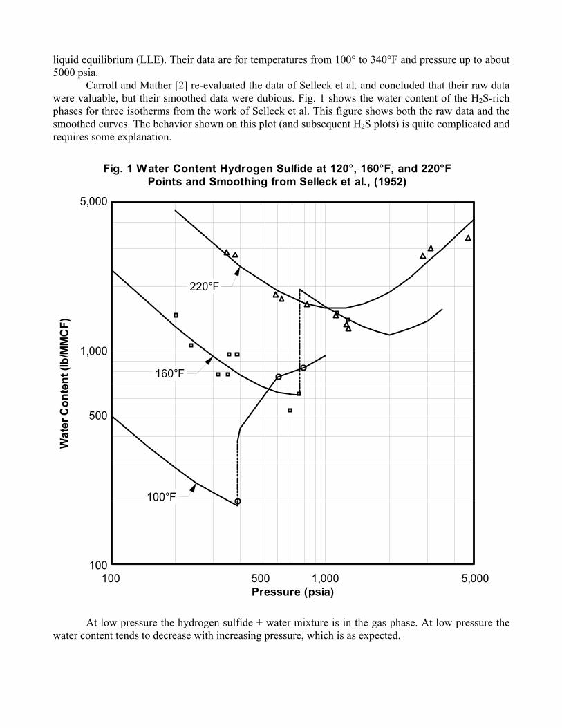
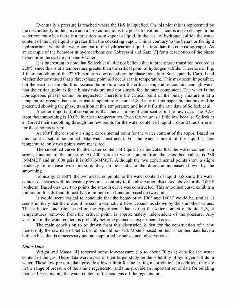
Carroll and Mather [2] re-evaluated the data of Selleck et al. and concluded that their raw datawere valuable, but their smoothed data were dubious. Fig. 1 shows the water content of the H2S-richphases for three isotherms from the work of Selleck et al. This figure shows both the raw data and thesmoothed curves. The behavior shown on this plot (and subsequent H2S plots) is quite complicated andrequires some explanation.
At low pressure the hydrogen sulfide + water mixture is in the gas phase. At low pressure thewater content tends to decrease with increasing pressure, which is as expected.
Pressure (psia)
Wat
er C
onte
nt (l
b/M
MC
F)
Fig. 1 Water Content Hydrogen Sulfide at 120°, 160°F, and 220°FPoints and Smoothing from Selleck et al., (1952)
100 500 1,000 5,000100
500
1,000
5,000
100°F
160°F
220°F
Eventually a pressure is reached where the H2S is liquefied. On this plot this is represented bythe discontinuity in the curve and a broken line joins the phase transition. There is a step change in thewater content when there is a transition from vapor to liquid. In the case of hydrogen sulfide the watercontent of the H2S liquid is greater than the coexisting vapor. This is contrary to the behavior for lighthydrocarbons where the water content in the hydrocarbon liquid is less than the coexisting vapor. Asan example of the behavior in hydrocarbons see Kobayashi and Katz [3] for a description of the phasebehavior in the system propane + water.
It is interesting to note that Selleck et al. did not believe that a three-phase transition occured at220°F since this is at a temperature greater than the critical point of hydrogen sulfide. Therefore in Fig.1 their smoothing of the 220°F isotherm does not show the phase transition. Subsequently Carroll andMather demonstrated that a three-phase point did occur at this temperature. This may seem impossible,but the reason is simple. It is because the mixture near the critical temperature contains enough waterthat the critical point is for a binary mixture and not simply for the pure component. The water is thenon-aqueous phases cannot be neglected. Therefore the critical point of the binary mixture is at atemperature greater than the critical temperature of pure H2S. Later in this paper predictions will bepresented showing the phase transition at this temperature and how it fits the raw data of Selleck et al.
Another important observation is that there is a significant scatter in the raw data. The AAEfrom their smoothing is 10.0% for these temperatures. Even this value is a little low because Selleck etal. forced their smoothing through the few points for the water content of liquid H2S and thus the errorfor these points is zero.
At 100°F there is only a single experimental point for the water content of the vapor. Based onthis point a set of smoothed data was constructed. For the water content of the liquid at thistemperature, only two points were measured.
The smoothed curve for the water content of liquid H2S indicates that the water content is astrong function of the pressure. At 400 psia the water content from the smoothed values is 380lb/MMCF and at 1000 psia it is 950 lb/MMCF. Although the two experimental points show a slighttendency to increase with pressure, they do not indicate the dramatic increases shown by thesmoothing.
Ironically, at 160°F the two measured points for the water content of liquid H2S show the watercontent decreases with increasing pressure – contrary to the observation discussed above for the 100°Fisotherm. Based on these two points the smooth curve was constructed. This smoothed curve exhibits aminimum. It is difficult to justify a minimum in a function based on two points.
It would seem logical to conclude that the behavior at 100° and 160°F would be similar. Itseems unlikely that there would be such a dramatic difference such as shown by the smoothed values.Thus a better conclusion based on the experimental data is that the water content of liquid H2S, attemperatures removed from the critical point, is approximately independent of the pressure. Anyvariation in the water content is probably better explained as experimental error.
The main conclusion to be drawn from this discussion is that for the construction of a newmodel only the raw data of Selleck et al. should be used. Models based on their smoothed data have abuilt-in bias that is unnecessary and not supported by subsequent observations.
Other DataWright and Maass [4] reported some low-pressure (up to about 70 psia) data for the water
content of the gas. These data were a part of their larger study on the solubility of hydrogen sulfide inwater. These low-pressure data provide a lower limit for the testing a correlation. In addition, they arein the range of pressure of the amine regenerator and thus provide an important set of data for buildingmodels for estimating the water content of the acid gas off the regenerator.
In addition, Gillespie et al. [5] measured VLE and LLE data for this system. Their data are forpressures up to 3000 psia. These data will be examined in a subsequent section of this paper. As willbe shown, these data are a key in revealing the true nature of the phase behavior in this system. It is thecombination of the data of Gillespie et al and the raw data of Selleck et al. along with a rigorousthermodynamic model that reveals the true nature of the phase behavior in the system hydrogen sulfide+ water.
Carbon DioxideIn general the phase behavior of the system carbon dioxide + water is as complex as that of the
system hydrogen sulfide + water. However for the range of temperature of this study a CO2-rich liquidphase is not encountered; it only occurs for temperatures less than about 90°F. On the other hand, thewater content of CO2 does exhibit a minimum.
For carbon dioxide + water the landmark study is that of Wiebe and Gaddy [6]. Included intheir study was the measurement of the water content of the CO2-rich phase for pressures up to 10,300psia.
Gillespie et al. [5] also measured phase equilibrium data for this system. In the range of interestin this study they measured the water content at two temperatures (167° and 200°F) and for pressurefrom 100 to about 3000 psia.
Two other important studies of the water content of CO2 are those of Coan and King [7] andKing et al. [8]. Coan and King included CO2 in their study of the water content of gases. Their data arefor temperatures up to 212°F and for pressure less than 750 psia. King et al. measured VLE in theregion near the critical point of CO2. Only one of their isotherms is in the region of interest in thisstudy (104°F) and it was for pressures up to about 3000 psia. However the rest of their data are animportant contribution as well.
There are a few low-pressure data for the water content of carbon dioxide in the temperaturerange of this study. Müller et al. [9] measured VLE at 212°F at pressures less than 340 psia. Zawiszaand Malesinska [10] measured two aqueous dew points at 212°F. Both of these papers contain muchmore data, but it is beyond the range of temperature of this study. As with the low pressure H2S data,these data are useful for testing low-pressure correlations, which in turn are useful for estimating thewater content of the acid gas off the amine regenerator.
Another important study of the water content of carbon dioxide is that of Song and Kobayashi[11]. They measured a few points for the phase equilibria for this system, however their points are allout of the range of temperature of interest in this work.
MethaneThe most important study of the aqueous dew points of pure methane is that of Olds et al. [12].
In this study they measured the dew point for pressures from 200 to 10,000 psia. Fortunately, the rawdata of Olds et al. are included in the published paper and thus are readily available. Olds et al. alsopublished tables of smoothed data.
There is some scatter in the raw data of Olds et al., the AE for their smoothing is 1.8% and theAAE is 5.2%. This provides a baseline for the comparison with other correlations.
In a study of the water content of gases Lukacs [13] measured the water content of puremethane at 160°F and pressures up to 1500 psia. Additional data from Lukacs will be examined in thesecond paper in this series.
As a part of their study, Gillespie at al. [5] also measured the water content of methane. In therange of interest in this study, they measured water content at 122° and 167°F and for pressures from200 to 2000 psia.
Rigby and Prausnitz [14] studied what they termed the solubility of water in compressed gases.One of the gases they studied was methane. Three of the isotherms they studied were in the region ofinterest in this study (122°, 167°, and 212°F). Their measurements were for pressures up to about 1000psia.
CALCULATING THE WATER CONTENT
There are several models available for calculating the water content of natural gas. Only a fewof them will be examined here.
In some of these models the vapor pressure of pure water is required as an input. Poor estimatesof the vapor pressure will lead to poor estimates of the water content. In this paper the vapor pressureis calculated using the correlation of Saul and Wagner [15].
Ideal ModelIn the Ideal Model, the water content of a gas is assumed to be equal to the vapor pressure of
pure water divided by the total pressure of the system. This yields the mole fraction of water in the gasand this is value converted to lb water per MMCF by multiplying by 47,484. Mathematically this is:
total
satwater
PP47484w = (1)
This equation yields w in lb/MMCF and the units on the two pressure terms must be the same; satwaterP is
the vapor pressure of pure water and Ptotal is the absolute pressure.Clearly this model is very simple and should not be expected to be highly accurate except at
very low pressures.A more thermodynamically correct model is to include the effect of gases dissolved in the
water. Mathematically this means:
total
satwaterwater
PPx47484w = (2)
In a typical application the solubility of the gas is not known and thus xwater is also unknown.Fortunately for hydrocarbons the solubility is so small that it is safe to assume that xwater equals unity.However, for acid gases, the solubility can be significant, even at relatively low pressure.
For the purposes of this paper, the Ideal Model is Eqn. (1).
McKetta-Wehe ChartIn 1958 McKetta and Wehe published a chart for estimating the water content of sweet natural
gas. This chart has been modified slightly over the years and has been reproduced in manypublications, most notably the GPSA Engineering Data Book [16].
To obtain the values in this study the original chart was photo-enlarged to two times its originalsize. Even so it is difficult to read the chart to an accuracy of more than two significant figures.Therefore the values reported here are only two significant figures.
The McKetta-Wehe chart is not applicable to sour gas, as will be clearly demonstrated here.Fortunately, most engineers who work in the natural gas industry are aware of this limitation. There
have been corrections proposed to make the chart applicable to these systems. Two will be discussedin the next paper in this series.
In addition, Kobayashi et al. [17] presented a correlation for the curves plotted in the McKetta-Wehe chart. Their equation is quite complicated and is only applicable for temperatures up to 120°Fand to 2000 psia. Therefore, this equation will not be discussed further.
Sharma-Campbell MethodSharma and Campbell [18] proposed a method for calculating the water content of natural gas,
including sour gas. Although originally designed for hand calculations, this method is rathercomplicated. It is even rather complicated for computer applications.
The method will be described here. Given the temperature and the pressure, the procedure is asfollows. Determine the fugacity if water at the saturation conditions (T and sat
waterP ), which is designatedsatwaterf , and the fugacity at the system conditions (T and Ptotal), designated fwater. A chart is provided to
estimate the fugacity of water at the system conditions. Then the correlation factor, k, is calculatedfrom the following equation:
0049.0
satwater
total
totalwater
satwater
satwater
total
satwater
PP
PfPf
PPk
= (3)
In this equation a consistent set of units should be used for the pressure and fugacity terms and then kis dimensionless. Then you must obtain the compressibility factor (z-factor), z, for the gas again atsystem conditions. They recommend using a generalized correlation for the compressibility. Finallythe water content is calculated as:
z
gas
satwater
ffk47484w
= (4)
where fgas is the fugacity of the dry gas calculated at system conditions. Again if a consistent set ofunits is used for the fugacity terms, then the calculated water content, w, is in lb/MMCF.
This method is rather difficult to use for hand calculations. First it requires the compressibilityfactor of the gas mixture. Next it requires the fugacity of pure water at system conditions. The chartgiven to estimate this value is only valid for temperatures between 80° and 160°F and for pressure lessthan 2000 psia. It is unclear how this method will behave if extrapolated beyond this range. Typicallythe calculation of a single fugacity is enough to scare away most process engineers. This methodrequires three fugacity calculations for a single water content estimate.
The pressure and temperature limitations make this method less useful for this study, where thepressure of interest ranges up to 10,000 psia and temperatures to 220°F. In addition, although this isintended to be a hand calculation method, it is a little difficult to use.
BukacekBukacek [19] suggested a relatively simple correlation for the water content of sweet gas. The
water content is calculated using an ideal contribution and a deviation factor. In equation form thecorrelation is as follows:
BPP47484w
total
satwater += (5)
69449.6t6.459
87.3083B ++
−=log (6)
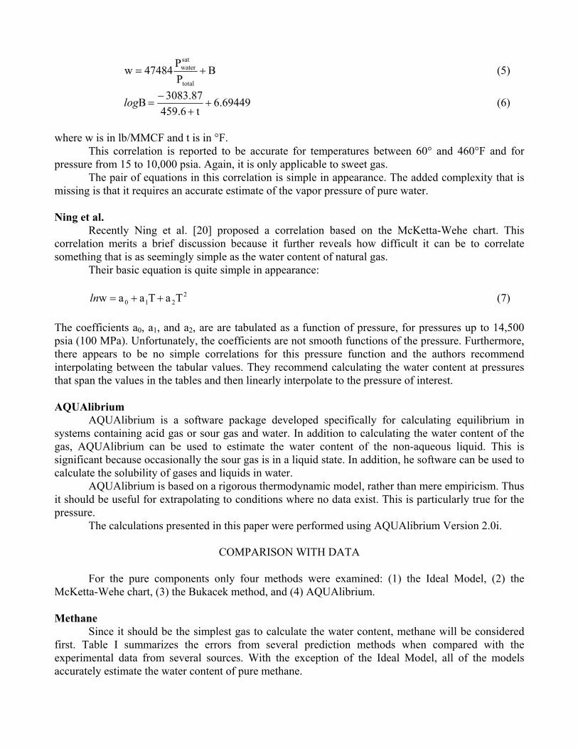
where w is in lb/MMCF and t is in °F.This correlation is reported to be accurate for temperatures between 60° and 460°F and for
pressure from 15 to 10,000 psia. Again, it is only applicable to sweet gas.The pair of equations in this correlation is simple in appearance. The added complexity that is
missing is that it requires an accurate estimate of the vapor pressure of pure water.
Ning et al.Recently Ning et al. [20] proposed a correlation based on the McKetta-Wehe chart. This
correlation merits a brief discussion because it further reveals how difficult it can be to correlatesomething that is as seemingly simple as the water content of natural gas.
Their basic equation is quite simple in appearance:
2210 TaTaaw ++=ln (7)
The coefficients a0, a1, and a2, are are tabulated as a function of pressure, for pressures up to 14,500psia (100 MPa). Unfortunately, the coefficients are not smooth functions of the pressure. Furthermore,there appears to be no simple correlations for this pressure function and the authors recommendinterpolating between the tabular values. They recommend calculating the water content at pressuresthat span the values in the tables and then linearly interpolate to the pressure of interest.
AQUAlibriumAQUAlibrium is a software package developed specifically for calculating equilibrium in
systems containing acid gas or sour gas and water. In addition to calculating the water content of thegas, AQUAlibrium can be used to estimate the water content of the non-aqueous liquid. This issignificant because occasionally the sour gas is in a liquid state. In addition, he software can be used tocalculate the solubility of gases and liquids in water.
AQUAlibrium is based on a rigorous thermodynamic model, rather than mere empiricism. Thusit should be useful for extrapolating to conditions where no data exist. This is particularly true for thepressure.
The calculations presented in this paper were performed using AQUAlibrium Version 2.0i.
COMPARISON WITH DATA
For the pure components only four methods were examined: (1) the Ideal Model, (2) theMcKetta-Wehe chart, (3) the Bukacek method, and (4) AQUAlibrium.
MethaneSince it should be the simplest gas to calculate the water content, methane will be considered
first. Table I summarizes the errors from several prediction methods when compared with theexperimental data from several sources. With the exception of the Ideal Model, all of the modelsaccurately estimate the water content of pure methane.
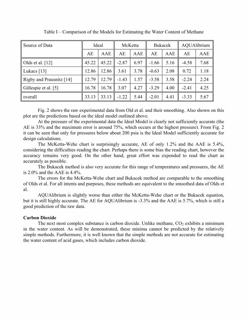
Table I – Comparison of the Models for Estimating the Water Content of Methane
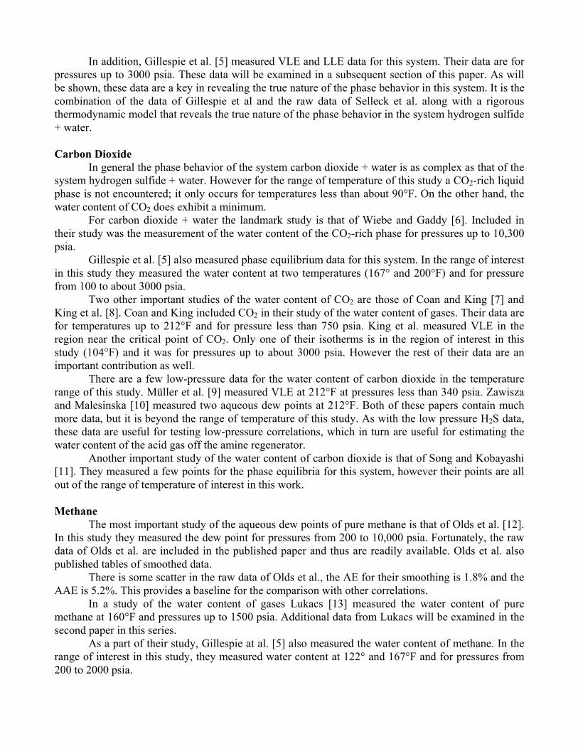
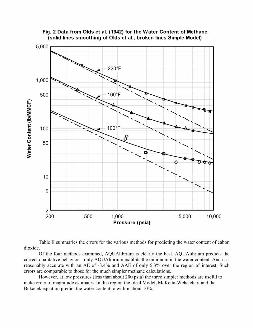
Fig. 2 shows the raw experimental data from Old et al. and their smoothing. Also shown on thisplot are the predictions based on the ideal model outlined above.
At the pressure of the experimental data the Ideal Model is clearly not sufficiently accurate (theAE is 33% and the maximum error is around 75%, which occurs at the highest pressure). From Fig. 2it can be seen that only for pressures below about 200 psia is the Ideal Model sufficiently accurate fordesign calculations.
The McKetta-Wehe chart is surprisingly accurate, AE of only 1.2% and the AAE is 5.4%,considering the difficulties reading the chart. Perhaps there is some bias the reading chart, however theaccuracy remains very good. On the other hand, great effort was expended to read the chart asaccurately as possible.
The Bukacek method is also very accurate for this range of temperatures and pressures, the AEis 2.0% and the AAE is 4.4%.
The errors for the McKetta-Wehe chart and Bukacek method are comparable to the smoothingof Olds et al. For all intents and purposes, these methods are equivalent to the smoothed data of Olds etal.
AQUAlibrium is slightly worse than either the McKetta-Wehe chart or the Bukacek equation,but it is still highly accurate. The AE for AQUAlibrium is -3.3% and the AAE is 5.7%, which is still agood prediction of the raw data.
Carbon DioxideThe next most complex substance is carbon dioxide. Unlike methane, CO2 exhibits a minimum
in the water content. As will be demonstrated, these minima cannot be predicted by the relativelysimple methods. Furthermore, it is well known that the simple methods are not accurate for estimatingthe water content of acid gases, which includes carbon dioxide.
Table II summaries the errors for the various methods for predicting the water content of cabondioxide.
Of the four methods examined, AQUAlibrium is clearly the best. AQUAlibrium predicts thecorrect qualitative behavior – only AQUAlibrium exhibits the minimum in the water content. And it isreasonably accurate with an AE of -3.4% and AAE of only 5.3% over the region of interest. Sucherrors are comparable to those for the much simpler methane calculations.
However, at low pressures (less than about 200 psia) the three simpler methods are useful tomake order of magnitude estimates. In this region the Ideal Model, McKetta-Wehe chart and theBukacek equation predict the water content to within about 10%.
Pressure (psia)
Wat
er C
onte
nt (l
b/M
MC
F)Fig. 2 Data from Olds et al. (1942) for the Water Content of Methane
(solid lines smoothing of Olds et al., broken lines Simple Model)
200 500 1,000 5,000 10,0002
5
10
50
100
500
1,000
5,000
100°F
160°F
220°F
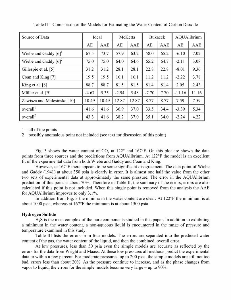
Table II – Comparison of the Models for Estimating the Water Content of Carbon Dioxide
1 – all of the points2 – possibly anomalous point not included (see text for discussion of this point)
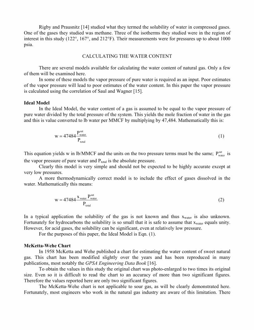
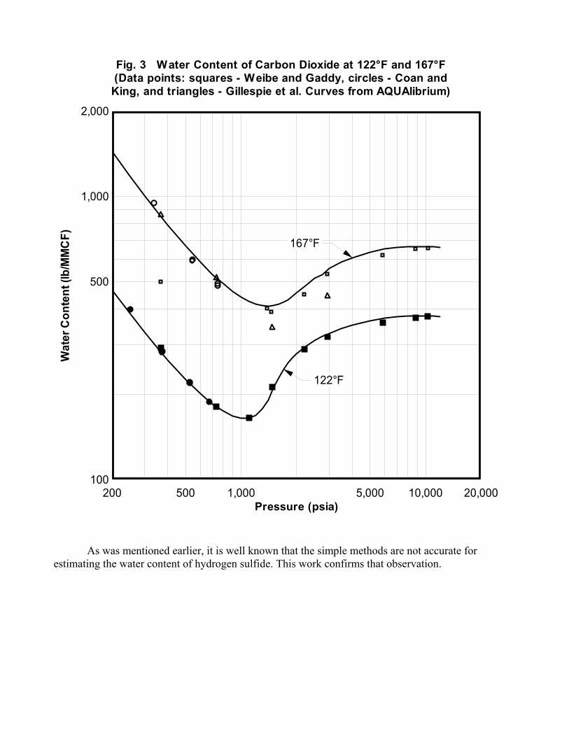
Fig. 3 shows the water content of CO2 at 122° and 167°F. On this plot are shown the datapoints from three sources and the predictions from AQUAlibrium. At 122°F the model is an excellentfit of the experimental data from both Wiebe and Gaddy and Coan and King.
However, at 167°F there appears to be some significant disagreement. The data point of Wiebeand Gaddy (1941) at about 350 psia is clearly in error. It is almost one half the value from the othertwo sets of experimental data at approximately the same pressure. The error in the AQUAlibriumprediction of this point is about 70%. Therefore in Table II, the summary of the errors, errors are alsocalculated if this point is not included. When this single point is removed from the analysis the AAEfor AQUAlibrium improves to only 3.1%.
In addition from Fig. 3 the minima in the water content are clear. At 122°F the minimum is atabout 1000 psia, whereas at 167°F the minimum is at about 1500 psia.
Hydrogen SulfideH2S is the most complex of the pure components studied in this paper. In addition to exhibiting
a minimum in the water content, a non-aqueous liquid is encountered in the range of pressure andtemperature examined in this study.
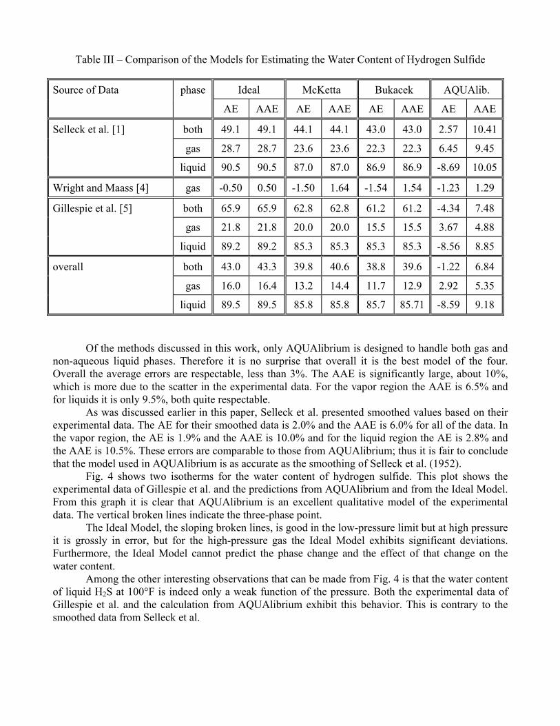
Table III lists the errors from four models. The errors are separated into the predicted watercontent of the gas, the water content of the liquid, and then the combined, overall error.
At low pressures, less than 50 psia even the simple models are accurate as reflected by theerrors for the data from Wright and Maass. At these low pressures all methods predict the experimentaldata to within a few percent. For moderate pressures, up to 200 psia, the simple models are still not toobad, errors less than about 20%. As the pressure continue to increase, and as the phase changes fromvapor to liquid, the errors for the simple models become very large – up to 90%.
As was mentioned earlier, it is well known that the simple methods are not accurate forestimating the water content of hydrogen sulfide. This work confirms that observation.
Pressure (psia)
Wat
er C
onte
nt (l
b/M
MC
F)Fig. 3 Water Content of Carbon Dioxide at 122°F and 167°F(Data points: squares - Weibe and Gaddy, circles - Coan and
King, and triangles - Gillespie et al. Curves from AQUAlibrium)
200 500 1,000 5,000 10,000 20,000100
500
1,000
2,000
122°F
167°F
Table III – Comparison of the Models for Estimating the Water Content of Hydrogen Sulfide
Source of Data phase Ideal McKetta Bukacek AQUAlib.
AE AAE AE AAE AE AAE AE AAE
Selleck et al. [1] both 49.1 49.1 44.1 44.1 43.0 43.0 2.57 10.41
gas 28.7 28.7 23.6 23.6 22.3 22.3 6.45 9.45
liquid 90.5 90.5 87.0 87.0 86.9 86.9 -8.69 10.05
Wright and Maass [4] gas -0.50 0.50 -1.50 1.64 -1.54 1.54 -1.23 1.29
Gillespie et al. [5] both 65.9 65.9 62.8 62.8 61.2 61.2 -4.34 7.48
gas 21.8 21.8 20.0 20.0 15.5 15.5 3.67 4.88
liquid 89.2 89.2 85.3 85.3 85.3 85.3 -8.56 8.85
overall both 43.0 43.3 39.8 40.6 38.8 39.6 -1.22 6.84
gas 16.0 16.4 13.2 14.4 11.7 12.9 2.92 5.35
liquid 89.5 89.5 85.8 85.8 85.7 85.71 -8.59 9.18
Of the methods discussed in this work, only AQUAlibrium is designed to handle both gas andnon-aqueous liquid phases. Therefore it is no surprise that overall it is the best model of the four.Overall the average errors are respectable, less than 3%. The AAE is significantly large, about 10%,which is more due to the scatter in the experimental data. For the vapor region the AAE is 6.5% andfor liquids it is only 9.5%, both quite respectable.
As was discussed earlier in this paper, Selleck et al. presented smoothed values based on theirexperimental data. The AE for their smoothed data is 2.0% and the AAE is 6.0% for all of the data. Inthe vapor region, the AE is 1.9% and the AAE is 10.0% and for the liquid region the AE is 2.8% andthe AAE is 10.5%. These errors are comparable to those from AQUAlibrium; thus it is fair to concludethat the model used in AQUAlibrium is as accurate as the smoothing of Selleck et al. (1952).
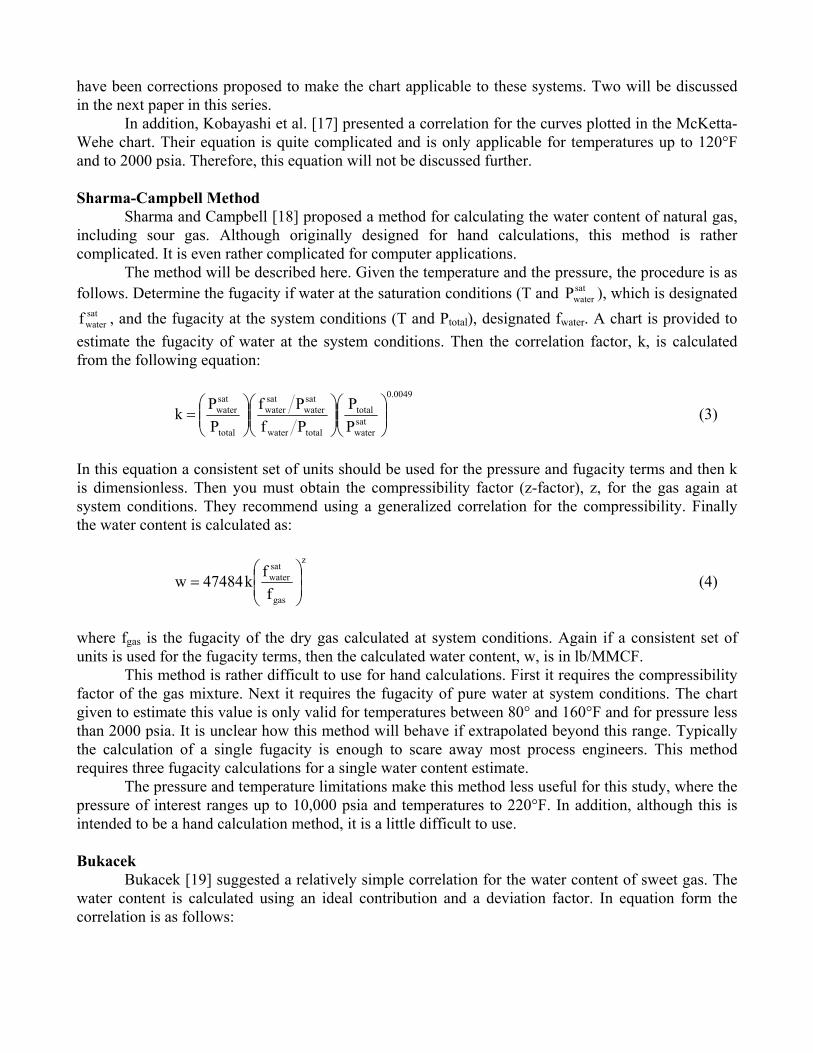
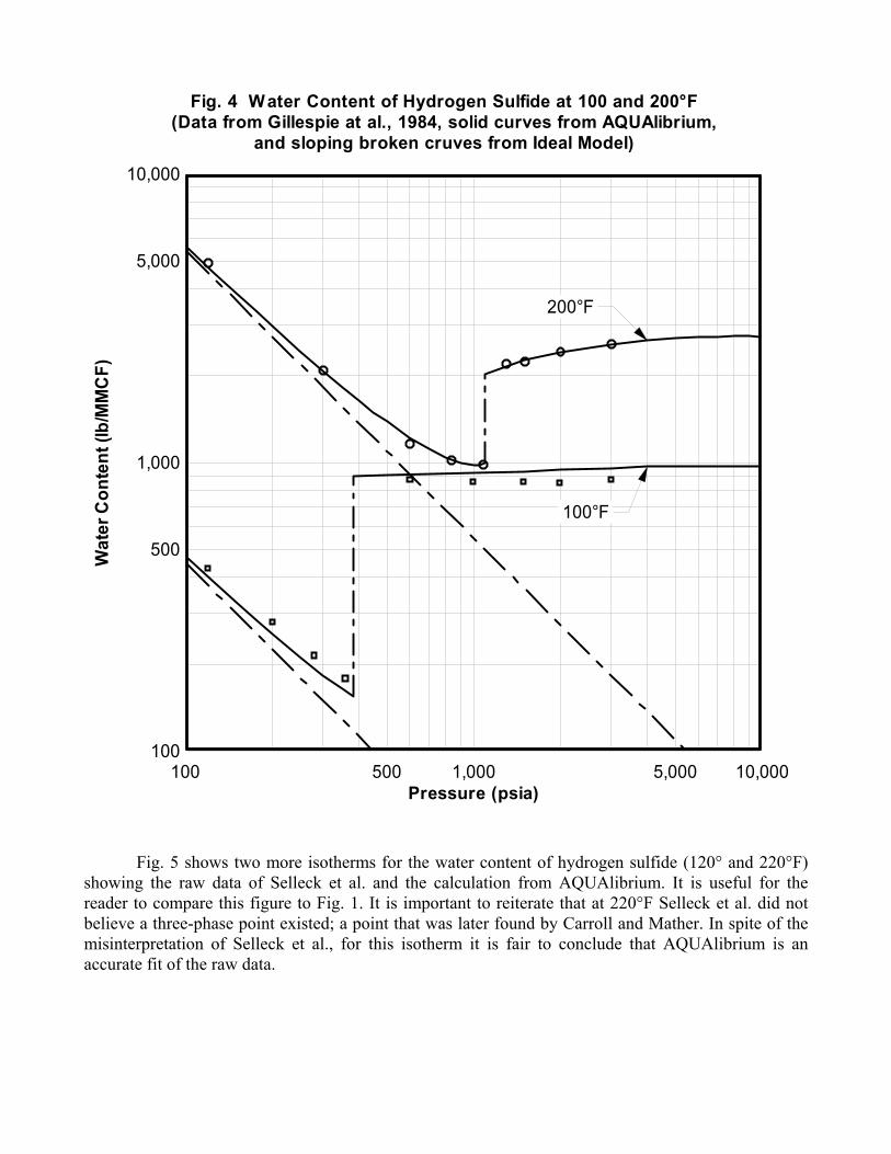
Fig. 4 shows two isotherms for the water content of hydrogen sulfide. This plot shows theexperimental data of Gillespie et al. and the predictions from AQUAlibrium and from the Ideal Model.From this graph it is clear that AQUAlibrium is an excellent qualitative model of the experimentaldata. The vertical broken lines indicate the three-phase point.
The Ideal Model, the sloping broken lines, is good in the low-pressure limit but at high pressureit is grossly in error, but for the high-pressure gas the Ideal Model exhibits significant deviations.Furthermore, the Ideal Model cannot predict the phase change and the effect of that change on thewater content.
Among the other interesting observations that can be made from Fig. 4 is that the water contentof liquid H2S at 100°F is indeed only a weak function of the pressure. Both the experimental data ofGillespie et al. and the calculation from AQUAlibrium exhibit this behavior. This is contrary to thesmoothed data from Selleck et al.
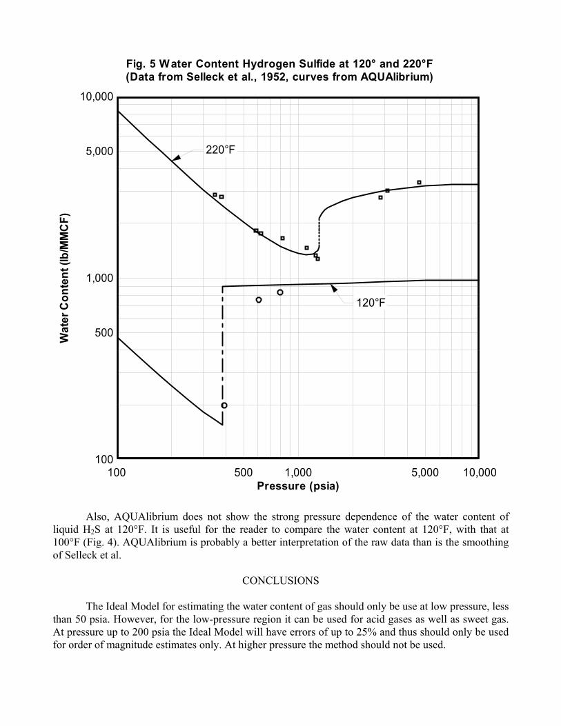
Fig. 5 shows two more isotherms for the water content of hydrogen sulfide (120° and 220°F)showing the raw data of Selleck et al. and the calculation from AQUAlibrium. It is useful for thereader to compare this figure to Fig. 1. It is important to reiterate that at 220°F Selleck et al. did notbelieve a three-phase point existed; a point that was later found by Carroll and Mather. In spite of themisinterpretation of Selleck et al., for this isotherm it is fair to conclude that AQUAlibrium is anaccurate fit of the raw data.
Pressure (psia)
Wat
er C
onte
nt (l
b/M
MC
F)Fig. 4 Water Content of Hydrogen Sulfide at 100 and 200°F
(Data from Gillespie at al., 1984, solid curves from AQUAlibrium,and sloping broken cruves from Ideal Model)
100 500 1,000 5,000 10,000100
500
1,000
5,000
10,000
200°F
100°F
Also, AQUAlibrium does not show the strong pressure dependence of the water content ofliquid H2S at 120°F. It is useful for the reader to compare the water content at 120°F, with that at100°F (Fig. 4). AQUAlibrium is probably a better interpretation of the raw data than is the smoothingof Selleck et al.
CONCLUSIONS
The Ideal Model for estimating the water content of gas should only be use at low pressure, lessthan 50 psia. However, for the low-pressure region it can be used for acid gases as well as sweet gas.At pressure up to 200 psia the Ideal Model will have errors of up to 25% and thus should only be usedfor order of magnitude estimates only. At higher pressure the method should not be used.
Pressure (psia)
Wat
er C
onte
nt (l
b/M
MC
F)Fig. 5 Water Content Hydrogen Sulfide at 120° and 220°F(Data from Selleck et al., 1952, curves from AQUAlibrium)
100 500 1,000 5,000 10,000100
500
1,000
5,000
10,000
220°F
120°F
However, this demonstrates that the Ideal Model does provide the correct limiting behavior,even for acid gases. Thus, any advanced model should also exhibit this limiting behavior.
As demonstrated in this paper, the methods of McKetta-Wehe and Bukacek are accurate forsweet gases throughout the range of pressure and temperature examined in this study. However, thesemethods are only accurate for low-pressure estimates when dealing with acid gas. These methodscannot handle the minimum in the water content observed in both H2S and CO2 and they cannot handlethe water content of the liquid, such as was demonstrated for H2S.
AQUAlibrium is accurate for all three scenarios – sweet gas, acid gas (including the minima inthe water content), and liquefied gases. Unlike the other models, AQUAlibrium was specificallydesigned to handle all three of these regions.
It is important to note that other software packages are available for predicting the watercontent of sweet gas, sour gas, and acid gas. The users of these programs should verify for themselvesthat the predictions are sufficiently accurate for their purposes.
REFERENCES CITED
1. Selleck, F.T., L.T. Carmichael, and B.H. Sage, “Phase Behavior in the Hydrogen Sulfide-WaterSystem” Ind. Eng. Chem. 44, 2219-2226 (1952).
2. Carroll, J.J. and A.E. Mather, “Phase Equilibrium in the System Water-Hydrogen Sulphide:Modelling the Phase Behaviour With an Equation of State” Can. J. Chem. Eng. 67, 999-1003(1989).
3. Kobayashi, R. and D.L. Katz, “Vapor-Liquid Equilibria for Binary Hydrocarbon-Water Systems”Ind. Eng. Chem., 45, 440-451 (1953).
4. Wright, R.H. and O. Maass, “The Solubility of Hydrogen Sulphide in Water from the VaporPressures of the Solutions” Can. J. Research 6, 94-101 (1932).
5. Gillespie, P.C., J.L. Owens, and G.M. Wilson, “Sour Water Equilibria Extended to HighTemperature and with Inerts Present” AIChE Winter National Meeting, Paper 34-b, Atlanta, GA,Mar. 11-14, (1984) and Gillespie, P.C. and G.M. Wilson, “Vapor-Liquid Equilibrium Data onWater-Substitute Gas Components: N2-H2O, H2-H2O, CO-H2O, H2-CO-H2O, and H2S-H2O”Research Report RR-41, GPA, Tulsa, OK, (1980)
6. Wiebe, R. and V.L. Gaddy, “Vapor Phase Composition of Carbon Dioxide-Water Mixtures atVarious Temperatures and at Pressures to 700 Atmospheres” J. Am. Chem. Soc. 63, 475-477(1941).
7. Coan, C.R. and A.D. King, “Solubility of Water in Compressed Carbon Dioxide, Nitrous Oxide,and Ethane. Evidence for Hydration of Carbon Dioxide and Nitrous Oxide in the Gas Phase” J.Am. Chem. Soc. 98, 1857-1862 (1971).
8. King, M.B., A. Mubarak, J.D. Kim, and T.R. Bott, “The Mutual Solubilities of Water withSupercritical and Liquid Carbon Dioxide” J. Supercritical Fluids 5, 296-302 (1992).
9. Müller, G., E. Bender, and G. Maurer, “Das Dampf-Flüssigkeitsgleichgewicht des ternärenSystems Ammoniak-Kohlendioxid-Wasser bei hohen Wassergehalten im Bereich zwischen 373und 473 Kelvin” Ber. Bunsenges. Phys. Chem. 92, 148-160 (1988).
10. Zawisza, A. and B. Malesinska, “Solubility of Carbon Dioxide in Liquid Water and of Water inGaseous Carbon Dioxide in the Range 0.2-5 MPa and at Temperatures up to 473 K” J. Chem. Eng.Data 26, 388-391 (1981)
11. Song, K.Y. and R. Kobayashi, “The Water Content of CO2-rich Fluids in Equilibrium with LiquidWater and/or Hydrates” Research Report RR-99, Gas Processors Association, Tulsa, OK, (1989).
12. Olds, R.H., B.H. Sage, and W.N. Lacey, “Phase Equilibria in Hydrocarbon Systems. Compositionof Dew-Point Gas in Methane-Water System” Ind. Eng. Chem. 34, 1223-1227 (1942).
13. Lukacs, J., Water Content of Hydrocarbon – Hydrogen Sulphide Gases, MSc Thesis, Dept. Chem.Eng., University of Alberta, Edmonton, AB, (1962) and Lukacs, J. and D.B. Robinson, “WaterContent of Sour Hydrocarbon Systems” Soc. Petrol. Eng. J. 3, 293-297 (1963).
14. Rigby, M. and J.M. Prausnitz, “Solubility of Water in Compressed Nitrogen, Argon, andMethane” J. Phys. Chem. 72, 330-334 (1968).
15. Saul, A. and W. Wagner, “International Equations for the Saturation Properties of Ordinary WaterSubstance” J. Phys. Chem. Ref. Data 16, 893-901 (1987).
16. ———, GPSA Engineering Data Book, 11th ed., Gas Processors Suppliers Association, Tulsa,OK, (1998).
17. Kobayashi, R., K.Y. Song, and E.D. Sloan, “Phase Behavior of Water/Hydrocarbon Systems” inBradley, H.B., (ed.), Petroleum Engineers Handbook, Society of Petroleum Engineers, Richardson,TX, (1987).
18. Sharma, S. and J.M. Campbell, “Predict Natural-gas Water Content with Total Gas Usage” Oil &Gas J., 136-137, Aug. 4, (1969).
19. Bukacek – quoted in McCain, W.D., The Properties of Petroleum Fluids, 2nd ed., PennWellBooks, Tulsa, OK, (1990).
20. Ning, Y., H. Zhang, and G. Zhou, “Mathematical Simulation and Program for Water ContentChart of Natural Gas” Chem. Eng. Oil Gas 29, 75-77 (2000). – in Chinese.
APPENDIX A – Definition of Error Estimates Used in this Paper
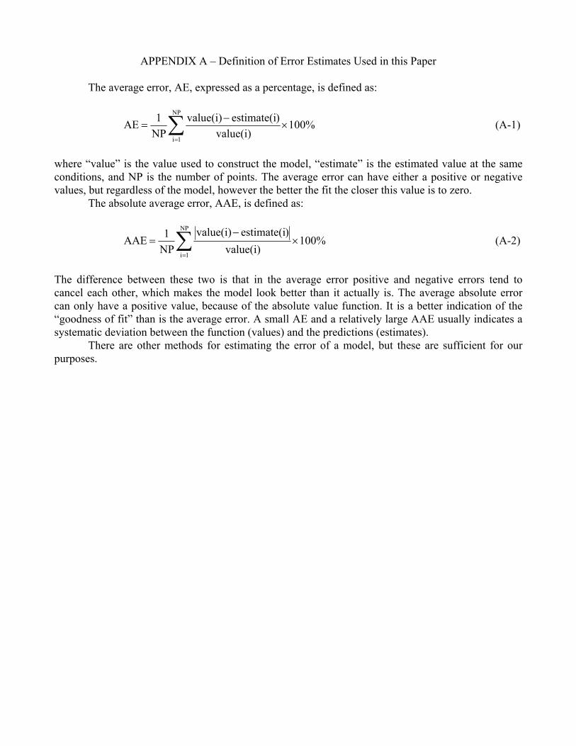
The average error, AE, expressed as a percentage, is defined as:
%100value(i)
)estimate(ivalue(i)NP1AE
NP
1i
×−
= ∑=
(A-1)
where “value” is the value used to construct the model, “estimate” is the estimated value at the sameconditions, and NP is the number of points. The average error can have either a positive or negativevalues, but regardless of the model, however the better the fit the closer this value is to zero.
The absolute average error, AAE, is defined as:
%100value(i)
)estimate(ivalue(i)NP1AAE
NP
1i
×−
= ∑=
(A-2)
The difference between these two is that in the average error positive and negative errors tend tocancel each other, which makes the model look better than it actually is. The average absolute errorcan only have a positive value, because of the absolute value function. It is a better indication of the“goodness of fit” than is the average error. A small AE and a relatively large AAE usually indicates asystematic deviation between the function (values) and the predictions (estimates).
There are other methods for estimating the error of a model, but these are sufficient for ourpurposes.
THE WATER CONTENT OF ACID GAS AND SOUR GAS FROM 100° TO220°F AND PRESSURES TO 10,000 PSIA. PART 2 – MIXTURES
John J. CarrollGas Liquids Engineering, Ltd.Calgary, Alberta, CANADA
ABSTRACT
The water content of the pure components is an interesting application and an importantprerequisite. However, it is almost always mixtures that are encountered in industrial practice. Thus, itis important to review the available data for mixtures and examine the accuracy of the methods forpredicting the water content of sour gas.
This paper, the second in the series, includes a discussion of the available experimental dataand comparison of a few available models. It will also include some discussion of the water content ofthe non-aqueous liquid phase, which may also be encountered in these mixtures. As with the previouspaper, this paper will be limited to temperatures from 100° to 220°F and for pressures up to 10,000psia.
Only limited data are available in the literature for the water content of sour gas mixtures. Thenew data of Ng et al. [1] will be reviewed. These data are an extensive new set of data covering a widerange of temperature and pressures and are for several compositions. However, other data will beexamined as well.
THE WATER CONTENT OF ACID GAS AND SOUR GAS FROM 100° TO220°F AND PRESSURES TO 10,000 PSIA PART 2 – MIXTURES
INTRODUCTION
As was discussed in the previous paper it is important for engineers to be able to accuratelypredict the water content of natural gas. The water content of sour gas, acid gas, and liquefied gasespose an additional problem.
LITERATURE REVIEW
There are only limited data available for the water content of mixture of the components thatcompose natural gas. This is especially true for sour gas mixtures. This makes such data quite valuable.
Lukacs [2] measured the water content for a few mixtures of methane and hydrogen sulfide at160°F at pressures up to 1400 psia. He also presented data for the water content of pure methane andthose data were examined in the first paper in this series. The errors in the water content for the data ofLukacs [2] were obtained by performing repeated measurements. For the sour gas mixtures, their watercontent mixtures are accurate to within ±3.5%, with a maximum error of 8%
Another interesting investigation was performed by Huang et al. [3]. They studied two mixturesof methane + carbon dioxide + hydrogen sulfide + water and their study included vapor-aqueousliquid, aqueous liquid-non-aqueous liquid and vapor-liquid-liquid equilibria. However only their watercontent data will be considered here.
The measurements of Huang et al. are at three temperatures: 100°, 225°, and 350°F. Althoughthe last two isotherms are outside the range of interest in this study, the second one is only slightly so.Thus the 225°F isotherm will be included in this analysis. Their data were for pressure from 700 to2500 psia. For the water composition they state that the measurements of the water concentration areaccurate to ±0.2 mol%, which is equivalent to ±95 lb/MMCF. This is a very large error for some of themeasurement. The measured water contents for the first mixture at 100°F are only approximately 90lb/MMCF. Perhaps this is a misprint and the errors are ±0.02 mol%, which would make the largesterrors on the order of ±10%. On the other hand several of the composition in this paper do not sum tounity. The error in the sum is as large as 0.32 mol%. In other measurements such an error may not besignificant but for these water content measurements this is quite large. For the calculations presentedthe compositions were first calculated on a water-free basis and the renormalized. The statedexperimental water mole fractions were converted to lb/MMCF without renormalizing.
Song and Kobayashi [4] reported some water content data for a mixture of CO2 (94.69 mol%)and methane (5.31 mol%). Although almost all of their data are outside the range of temperature ofinterest in this work, this is interesting set of data, which demonstrate the effect of a relatively smallamount of methane on the water content of CO2.
Recently Ng et al. [1] published a set of VLE data for sour gas mixtures at 120° and 200°F andpressures from 200 to 10,000 psia. Because of the range of temperature and pressure covered by theseexperiments, they are a significant contribution to the literature. In addition to presenting water contentinformation, these data also include measurements of the solubility of gas mixtures in water and thedensities of the equilibrium phases. However, in this paper only their water content data will beexamined. Finally, a detailed discussion of the errors with these data is presented later in this paper.
CALCULATING THE WATER CONTENT
Methods for calculating the water content of natural gas were presented in the previous paperand therefore will not be repeated here. Most of those methods were specifically designed for sweetgas systems. The reader is referred to the first paper for the details of those methods. Some of thosemethods will be used for predicting the water content of the mixtures examined in this paper.
In addition there are some methods that are specifically designed for estimating the watercontent of sour gas mixtures. They will be reviewed briefly in the sections that follow.
Maddox CorrectionMaddox [5] developed a method for estimating the water content of sour natural gas. His
method assumes that the water content of sour gas is the sum of three terms: 1. a sweet gascontribution, 2. a contribution from CO2, and 3. a contribution form H2S.
The water content of the gas is calculated as a mole fraction weighted average of the threecontributions.
SHSHCOCOHCHC 2222wywywyw ++= (1)
where w is the water content, y is the mole fraction, the subscript HC refers to hydrocarbon, CO2 iscarbon dioxide and H2S is hydrogen sulfide. Charts are provided to estimate the contributions for CO2and H2S. The chart for CO2 is for temperatures between 80° and 160°F and the chart for H2S is for 80°and 280°F. Both charts are for pressures from 100 to 3000 psia.
To use this method, one finds the water content of sweet gas, typically from the McKetta-Wehechart then the corrections for the acid gases are obtained from their respective charts.
Although these charts have the appearance of being useful for calculating the water content ofpure H2S and pure CO2 the author advises that they should not be used for this purpose.
In the appendix of this paper the charts are converted into mathematical expressions that canthen be used for computer calculations. Finally a computer program was written that combined thesweet gas estimate from Bukacek (see Part 1 of this series of papers) and the correlations of theMaddox correction.
Robinson et al. ChartsRobinson et al. [6] used an equation of state method to calculate the water content of sour
natural gases. Using their equation of state model they generate a series of charts; one chart for 300,1000, 2000, 300, 6000, and 10,000 psia. The temperature range for the charts is 50° to 350°F, althoughit is slightly narrower at some pressures. A third parameter on the chart is the H2S equivalent and iscalculated as follows:
222 COSHequiv
SH y75.0yy += (2)
The charts are applicable for H2S equivalent up to 40 mole %.These charts remain popular, but they require multiple interpolations, which makes them a little
difficult to use. This method will not be examined in detail in this paper.
Wichert CorrectionWichert and Wichert [7] proposed a relatively simple correction based on the equivalent H2S
content of the gas. The equivalent H2S content used in this correlation is that defined by Eqn. (2).They presented a single chart where given the temperature pressure and equivalent H2S one
could obtain a correction factor, Fcorr. Correction factors range from 0.95 to 5.0. The correction factorstend to increase with increasing H2S equivalent and increasing pressure, and decrease with increasingtemperature.
The water content of the sour gas is calculated as follows:
WMcorrwFw −= (3)
where w is the water content of the sour gas, Fcorr the a correction factor, and wM-W is the water contentof sweet gas from the McKetta-Wehe chart. Fcorr is dimensionless so the two water content termssimply have the same units, typically lb/MMCF, in order to be dimensionally consistent.
This method is limited to an H2S equivalent of 55 mol% and is applicable for temperaturesfrom 50° to 350°F and pressure from 200 to 10,000 psia.
This method is much simpler to use than the charts of Robinson et al. [6] since it does notrequire the interpolations of the earlier method.
AQUAlibriumAQUAlibrium was introduced in Part 1 of this series of papers. It will be used in this paper for
estimating the water content of mixtures. One advantage of AQUAlibrium over the simpler methods isthat AQUAlibrium is applicable for calculating the water content of both the gas and the non-aqueousliquid phases. The simple methods cannot be used to predict the water content of a non-aqueous liquid.
All of the calculations presented in this paper were performed using AQUAlibrium Version2.0i.
WATER CONTENT OF MIXTURES
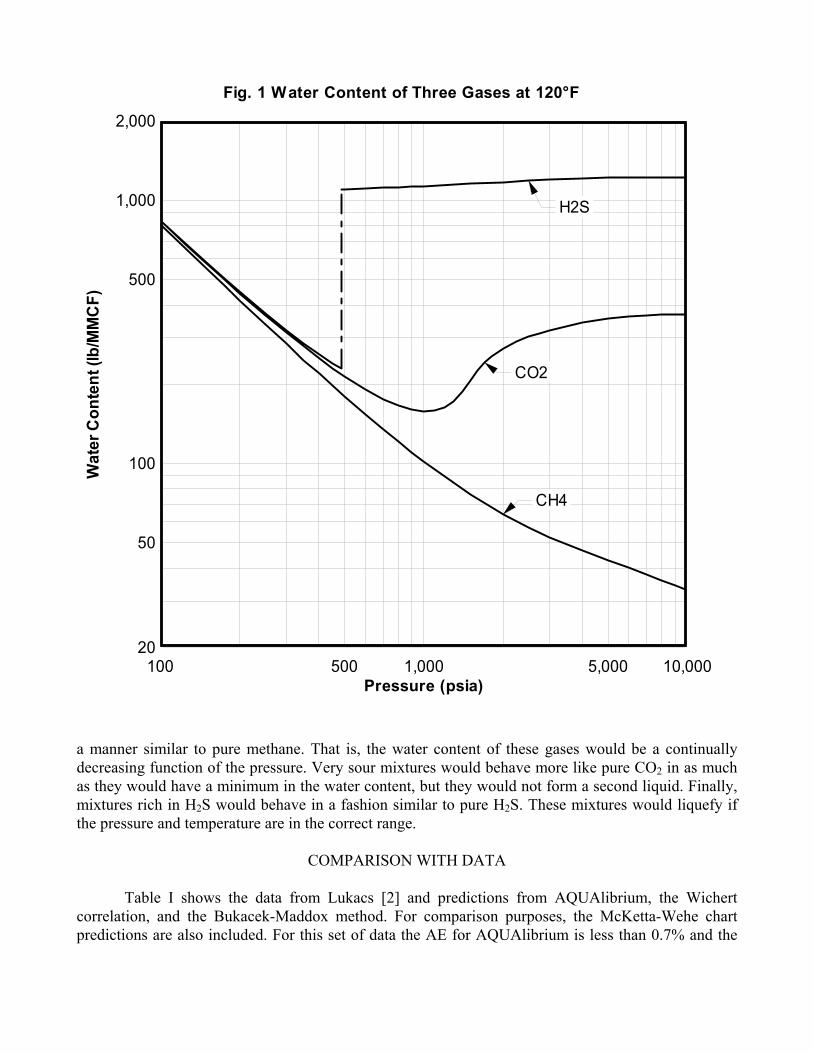
Fig. 1 shows the water content of methane, carbon dioxide, and hydrogen sulfide at 120°F. Thecurves were calculated using AQUAlibrium and the accuracy of this method for these components wasdemonstrated in the first paper in this series. This figure shows the diversity of behavior that occurs.
At low pressure the water content is essentially the same for all three substances. At these lowpressures the water content is a function of the temperature and pressure and is accurately predictedusing the ideal model. As the pressure increases the phase behavior for the three substances issignificantly different.
The water content of methane, as an example of sweet gas, continually decreases as thepressure increases. This is reflected in the McKetta-Wehe chart for estimating the water content ofsweet gas, which was demonstrated to be highly accurate for estimating the water content of methane.
On the other hand, the water content of carbon dioxide exhibits a minimum. This ischaracteristic of acid gases and very sour gas mixtures.
Finally hydrogen sulfide liquefies. For this reason the water content of hydrogen sulfideexhibits a discontinuity. Carbon dioxide behaves similarly, but at lower temperature. The temperaturesat which a CO2-rich liquid forms is outside the range of interest here.
It is logical to assume that the behavior of the mixtures would have characteristics of the threepure components. Sour gas mixtures that contain only a small amount of CO2 and H2S would behave in
a manner similar to pure methane. That is, the water content of these gases would be a continuallydecreasing function of the pressure. Very sour mixtures would behave more like pure CO2 in as muchas they would have a minimum in the water content, but they would not form a second liquid. Finally,mixtures rich in H2S would behave in a fashion similar to pure H2S. These mixtures would liquefy ifthe pressure and temperature are in the correct range.
COMPARISON WITH DATA
Table I shows the data from Lukacs [2] and predictions from AQUAlibrium, the Wichertcorrelation, and the Bukacek-Maddox method. For comparison purposes, the McKetta-Wehe chartpredictions are also included. For this set of data the AE for AQUAlibrium is less than 0.7% and the
Pressure (psia)
Wat
er C
onte
nt (l
b/M
MC
F)Fig. 1 Water Content of Three Gases at 120°F
100 500 1,000 5,000 10,00020
50
100
500
1,000
2,000
H2S
CO2
CH4
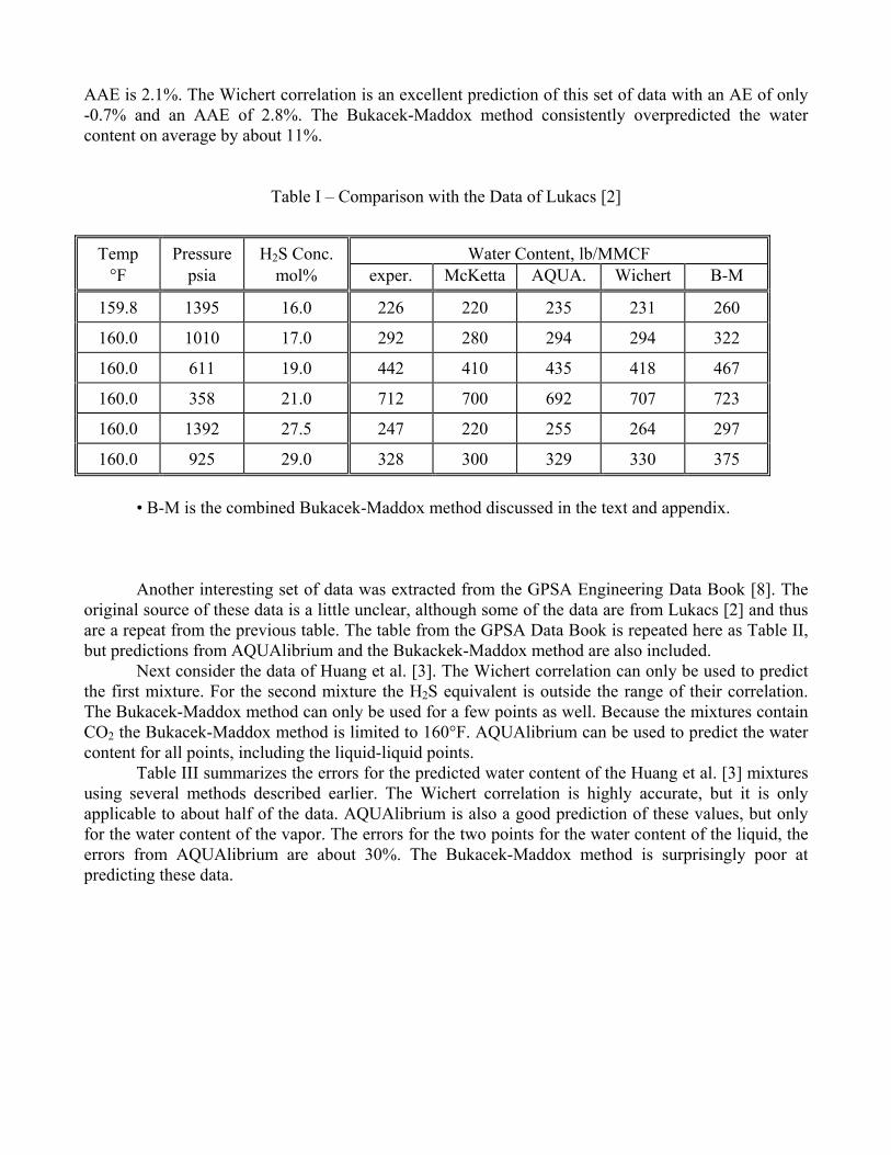
AAE is 2.1%. The Wichert correlation is an excellent prediction of this set of data with an AE of only-0.7% and an AAE of 2.8%. The Bukacek-Maddox method consistently overpredicted the watercontent on average by about 11%.
• B-M is the combined Bukacek-Maddox method discussed in the text and appendix.
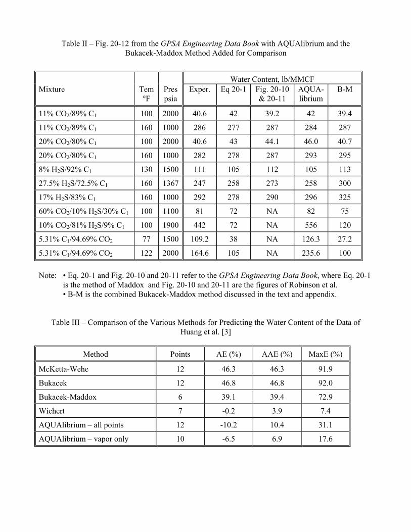
Another interesting set of data was extracted from the GPSA Engineering Data Book [8]. Theoriginal source of these data is a little unclear, although some of the data are from Lukacs [2] and thusare a repeat from the previous table. The table from the GPSA Data Book is repeated here as Table II,but predictions from AQUAlibrium and the Bukackek-Maddox method are also included.
Next consider the data of Huang et al. [3]. The Wichert correlation can only be used to predictthe first mixture. For the second mixture the H2S equivalent is outside the range of their correlation.The Bukacek-Maddox method can only be used for a few points as well. Because the mixtures containCO2 the Bukacek-Maddox method is limited to 160°F. AQUAlibrium can be used to predict the watercontent for all points, including the liquid-liquid points.
Table III summarizes the errors for the predicted water content of the Huang et al. [3] mixturesusing several methods described earlier. The Wichert correlation is highly accurate, but it is onlyapplicable to about half of the data. AQUAlibrium is also a good prediction of these values, but onlyfor the water content of the vapor. The errors for the two points for the water content of the liquid, theerrors from AQUAlibrium are about 30%. The Bukacek-Maddox method is surprisingly poor atpredicting these data.
Table II – Fig. 20-12 from the GPSA Engineering Data Book with AQUAlibrium and theBukacek-Maddox Method Added for Comparison
Water Content, lb/MMCFMixture Tem
°FPrespsia
Exper. Eq 20-1 Fig. 20-10& 20-11
AQUA-librium
B-M
11% CO2/89% C1 100 2000 40.6 42 39.2 42 39.4
11% CO2/89% C1 160 1000 286 277 287 284 287
20% CO2/80% C1 100 2000 40.6 43 44.1 46.0 40.7
20% CO2/80% C1 160 1000 282 278 287 293 295
8% H2S/92% C1 130 1500 111 105 112 105 113
27.5% H2S/72.5% C1 160 1367 247 258 273 258 300
17% H2S/83% C1 160 1000 292 278 290 296 325
60% CO2/10% H2S/30% C1 100 1100 81 72 NA 82 75
10% CO2/81% H2S/9% C1 100 1900 442 72 NA 556 120
5.31% C1/94.69% CO2 77 1500 109.2 38 NA 126.3 27.2
5.31% C1/94.69% CO2 122 2000 164.6 105 NA 235.6 100
Note: • Eq. 20-1 and Fig. 20-10 and 20-11 refer to the GPSA Engineering Data Book, where Eq. 20-1is the method of Maddox and Fig. 20-10 and 20-11 are the figures of Robinson et al.• B-M is the combined Bukacek-Maddox method discussed in the text and appendix.
Table III – Comparison of the Various Methods for Predicting the Water Content of the Data ofHuang et al. [3]
Method Points AE (%) AAE (%) MaxE (%)
McKetta-Wehe 12 46.3 46.3 91.9
Bukacek 12 46.8 46.8 92.0
Bukacek-Maddox 6 39.1 39.4 72.9
Wichert 7 -0.2 3.9 7.4
AQUAlibrium – all points 12 -10.2 10.4 31.1
AQUAlibrium – vapor only 10 -6.5 6.9 17.6
Data of Ng et al.The new data from Ng et al. [1] are an important set and deserve special treatment. Most of
these data are for the quinary system: water, methane, propane, hydrogen sulfide, and carbon dioxide.There are some data for an eight-component mixture as well.
In the analysis of the water content of the gas, the mole fraction water in the measuredcomposition was removed and then the composition was normalized to obtain the water-freecomposition. The mole fraction water in the gas was then converted to a lb/MMCF equivalent.
In addition, two mixtures deserve special considerations. These mixtures are those designated5HC-95AC2 and 5HC-95AC3 by the authors and are very rich in the acid gas components. The firstmixture has an estimated critical temperature of approximately 120°F. Therefore the 120°F data pointsare nearly at the critical temperature. The critical region is typically difficult for performingequilibrium calculations. Thus these points present a significant challenge. The second mixture has anestimated critical temperature of approximately 160°F. Therefore, the three high pressure points for thethis mixture at 120°F are liquid-liquid equilibrium points.
The 200 psia IsobarFrom the analysis of the pure component data it was concluded that to within about 10% the
water content at 200 psia is independent of the component. This assumption was extrapolated tomixtures based on this observation and based on the current models for water content. For example theWichert correlation indicates that at 200 psia the water content of a sour gas at 200 psia for sour gas iswithin 5% of the value for sweet gas.
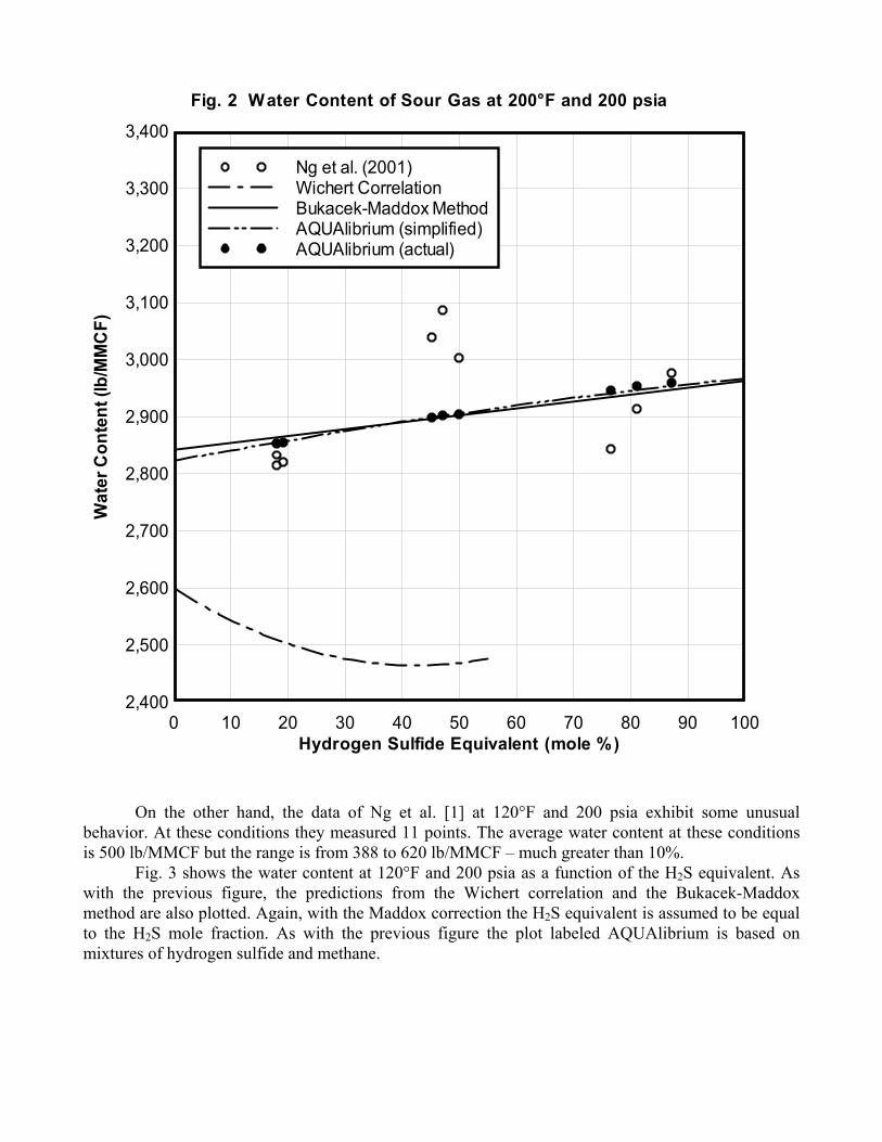
First consider the data at 200°F and 200 psia. Ng et al. [1] measured 9 points at theseconditions. The average water content for these points is 2930 lb/MMCF and the range of experimentalwater content is less than 10%. As a function of H2S equivalent the experimental points show amaximum water content at approximately 60 mol%, although such a conclusion may not be justifiedfrom the data. These data reinforce the observation stated earlier regarding low pressure water content.
Fig. 2 shows the experimental water content at 200°F and 200 psia as a function of H2Sequivalent. Shown on this plot is the prediction from the Wichert correlation. Note at these conditionsthe Wichert correlation predicts that the water content decreases with increasing H2S equivalent. It alsoappears that the McKetta-Wehe point for sweet gas is a little low at these conditions, but a closereview of the chart indicates that the water content at 200°F and 200 psia is 2600 lb/MMCF.
Also shown on this plot is the Bukacek-Maddox correlation, which was constructed assumingthat the H2S equivalent was equal to the H2S mole fraction. This method predicts the experimental dataof Ng et al. [1] at 200°F and 200 psia to within better than 10%. It is worth noting that these conditionsare outside the range for the CO2 contribution for the Maddox correction, so this correlation probablyshould not have been used for this example.
In addition predictions from AQUAlibrium are also presented. The curve labeledAQUAlibrium (simplified) on Fig. 2 was constructed based on mixtures of methane + hydrogensulfide. The points labeled AQUAlibrium (actual) are the values calculated using the experimentalcompositions. At these conditions the simplified and actual are approximately coincident.
Furthermore, It is clear from this plot that this prediction from AQUAlibrium and the Bukacek-Maddox method are essentially equivalent.
However, from all of this it is fair to conclude that this reinforces the observation regarding thecomposition effect at 200 psia. That is, to within ±10% the water content is independent of thecomposition at 200 psia.
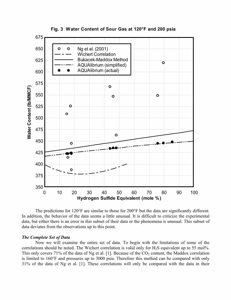
On the other hand, the data of Ng et al. [1] at 120°F and 200 psia exhibit some unusualbehavior. At these conditions they measured 11 points. The average water content at these conditionsis 500 lb/MMCF but the range is from 388 to 620 lb/MMCF – much greater than 10%.
Fig. 3 shows the water content at 120°F and 200 psia as a function of the H2S equivalent. Aswith the previous figure, the predictions from the Wichert correlation and the Bukacek-Maddoxmethod are also plotted. Again, with the Maddox correction the H2S equivalent is assumed to be equalto the H2S mole fraction. As with the previous figure the plot labeled AQUAlibrium is based onmixtures of hydrogen sulfide and methane.
Hydrogen Sulfide Equivalent (mole %)
Wat
er C
onte
nt (l
b/M
MC
F)Fig. 2 Water Content of Sour Gas at 200°F and 200 psia
0 10 20 30 40 50 60 70 80 90 1002,400
2,500
2,600
2,700
2,800
2,900
3,000
3,100
3,200
3,300
3,400
Ng et al. (2001) Wichert Correlation Bukacek-Maddox Method AQUAlibrium (simplified) AQUAlibrium (actual)
The predictions for 120°F are similar to those for 200°F but the data are significantly different.In addition, the behavior of the data seems a little unusual. It is difficult to criticize the experimentaldata, but either there is an error in this subset of their data or the phenomena is unusual. This subset ofdata deviates from the observations up to this point.
The Complete Set of DataNow we will examine the entire set of data. To begin with the limitations of some of the
correlations should be noted. The Wichert correlation is valid only for H2S equivalent up to 55 mol%.This only covers 71% of the data of Ng et al. [1]. Because of the CO2 content, the Maddox correlationis limited to 160°F and pressures up to 3000 psia. Therefore this method can be compared with only31% of the data of Ng et al. [1]. These correlations will only be compared with the data in their
Hydrogen Sulfide Equivalent (mole %)
Wat
er C
onte
nt (l
b/M
MC
F)Fig. 3 Water Content of Sour Gas at 120°F and 200 psia
0 10 20 30 40 50 60 70 80 90 100350
375
400
425
450
475
500
525
550
575
600
625
650
675
Ng et al. (2001) Wichert Correlation Bukacek-Maddox Method AQUAlibrium (simplified) AQUAlibrium (actual)
specified ranges. AQUAlibrium is not limited by pressures, temperature, or composition and thus willbe compared with all of the data.
The errors for the various methods are listed in Table IV. However, this information does notcompletely reveal the details of the various prediction methods. Therefore these predictions should beexamined in more detail.
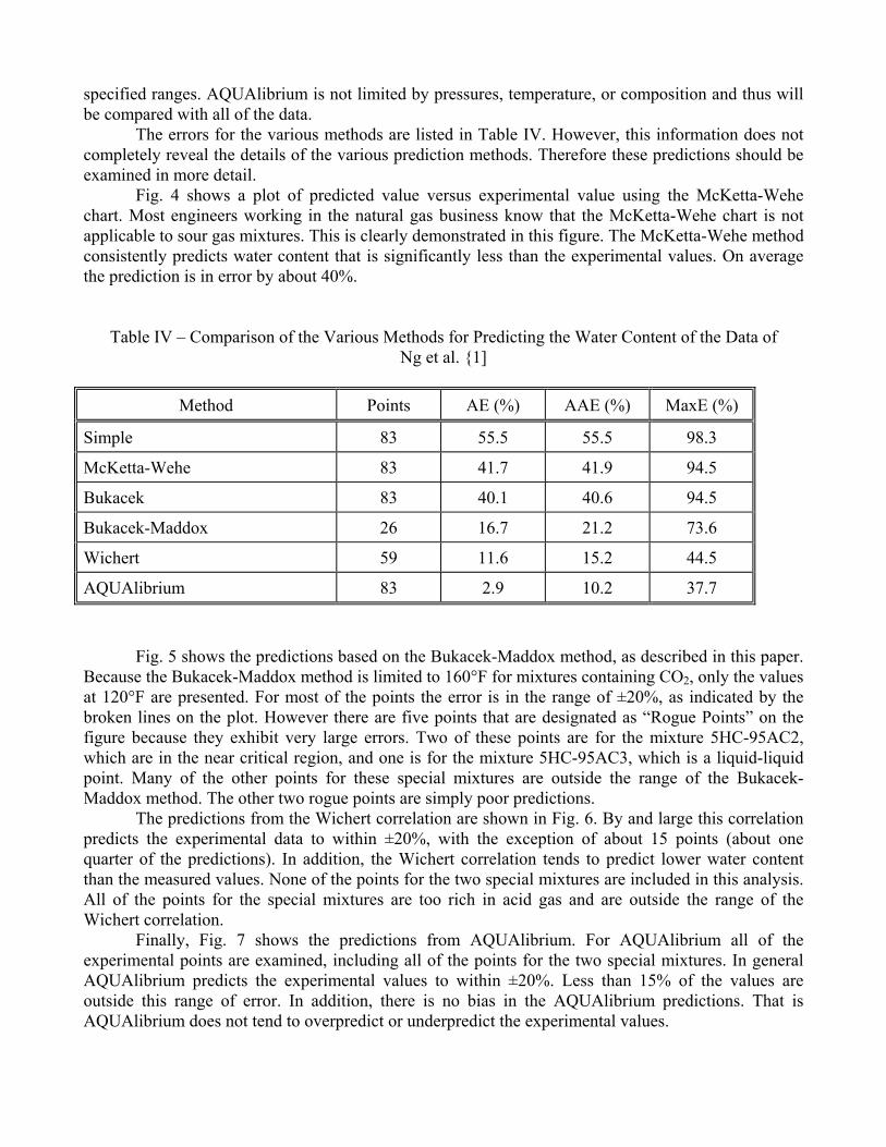
Fig. 4 shows a plot of predicted value versus experimental value using the McKetta-Wehechart. Most engineers working in the natural gas business know that the McKetta-Wehe chart is notapplicable to sour gas mixtures. This is clearly demonstrated in this figure. The McKetta-Wehe methodconsistently predicts water content that is significantly less than the experimental values. On averagethe prediction is in error by about 40%.
Table IV – Comparison of the Various Methods for Predicting the Water Content of the Data ofNg et al. {1]
Method Points AE (%) AAE (%) MaxE (%)
Simple 83 55.5 55.5 98.3
McKetta-Wehe 83 41.7 41.9 94.5
Bukacek 83 40.1 40.6 94.5
Bukacek-Maddox 26 16.7 21.2 73.6
Wichert 59 11.6 15.2 44.5
AQUAlibrium 83 2.9 10.2 37.7
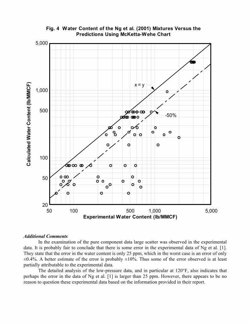
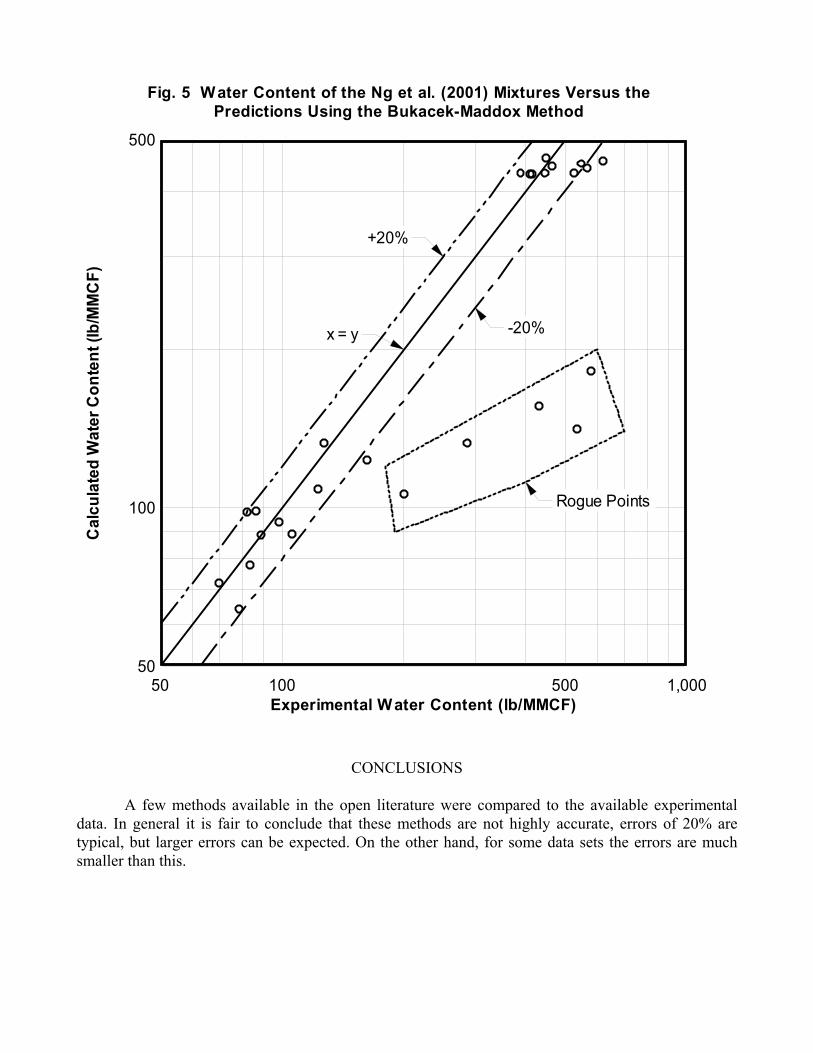
Fig. 5 shows the predictions based on the Bukacek-Maddox method, as described in this paper.Because the Bukacek-Maddox method is limited to 160°F for mixtures containing CO2, only the valuesat 120°F are presented. For most of the points the error is in the range of ±20%, as indicated by thebroken lines on the plot. However there are five points that are designated as “Rogue Points” on thefigure because they exhibit very large errors. Two of these points are for the mixture 5HC-95AC2,which are in the near critical region, and one is for the mixture 5HC-95AC3, which is a liquid-liquidpoint. Many of the other points for these special mixtures are outside the range of the Bukacek-Maddox method. The other two rogue points are simply poor predictions.
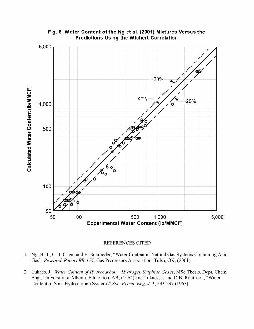
The predictions from the Wichert correlation are shown in Fig. 6. By and large this correlationpredicts the experimental data to within ±20%, with the exception of about 15 points (about onequarter of the predictions). In addition, the Wichert correlation tends to predict lower water contentthan the measured values. None of the points for the two special mixtures are included in this analysis.All of the points for the special mixtures are too rich in acid gas and are outside the range of theWichert correlation.
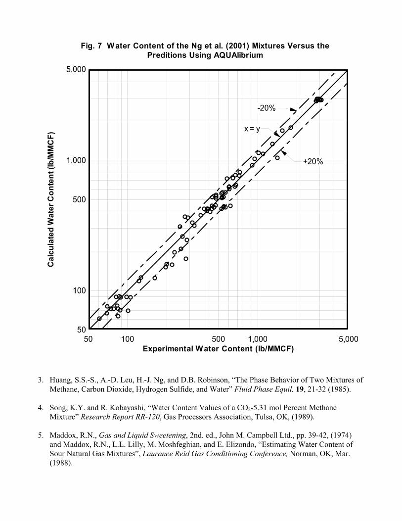
Finally, Fig. 7 shows the predictions from AQUAlibrium. For AQUAlibrium all of theexperimental points are examined, including all of the points for the two special mixtures. In generalAQUAlibrium predicts the experimental values to within ±20%. Less than 15% of the values areoutside this range of error. In addition, there is no bias in the AQUAlibrium predictions. That isAQUAlibrium does not tend to overpredict or underpredict the experimental values.
Additional CommentsIn the examination of the pure component data large scatter was observed in the experimental
data. It is probably fair to conclude that there is some error in the experimental data of Ng et al. [1].They state that the error in the water content is only 25 ppm, which in the worst case is an error of only±0.4%. A better estimate of the error is probably ±10%. Thus some of the error observed is at leastpartially attributable to the experimental data.
The detailed analysis of the low-pressure data, and in particular at 120°F, also indicates thatperhaps the error in the data of Ng et al. [1] is larger than 25 ppm. However, there appears to be noreason to question these experimental data based on the information provided in their report.
Experimental Water Content (lb/MMCF)
Cal
cula
ted
Wat
er C
onte
nt (l
b/M
MC
F)Fig. 4 Water Content of the Ng et al. (2001) Mixtures Versus the
Predictions Using McKetta-Wehe Chart
50 100 500 1,000 5,00020
50
100
500
1,000
5,000
x = y
-50%
CONCLUSIONS
A few methods available in the open literature were compared to the available experimentaldata. In general it is fair to conclude that these methods are not highly accurate, errors of 20% aretypical, but larger errors can be expected. On the other hand, for some data sets the errors are muchsmaller than this.
Experimental Water Content (lb/MMCF)
Cal
cula
ted
Wat
er C
onte
nt (l
b/M
MC
F)Fig. 5 Water Content of the Ng et al. (2001) Mixtures Versus the
Predictions Using the Bukacek-Maddox Method
50 100 500 1,00050
100
500
x = y
Rogue Points
+20%
-20%
REFERENCES CITED
1. Ng, H.-J., C.-J. Chen, and H. Schroeder, “Water Content of Natural Gas Systems Containing AcidGas”, Research Report RR-174, Gas Processors Association, Tulsa, OK, (2001).
2. Lukacs, J., Water Content of Hydrocarbon – Hydrogen Sulphide Gases, MSc Thesis, Dept. Chem.Eng., University of Alberta, Edmonton, AB, (1962) and Lukacs, J. and D.B. Robinson, “WaterContent of Sour Hydrocarbon Systems” Soc. Petrol. Eng. J. 3, 293-297 (1963).
Experimental Water Content (lb/MMCF)
Cal
cula
ted
Wat
er C
onte
nt (l
b/M
MC
F)Fig. 6 Water Content of the Ng et al. (2001) Mixtures Versus the
Predictions Using the Wichert Correlation
50 100 500 1,000 5,00050
100
500
1,000
5,000
x = y
+20%
-20%
3. Huang, S.S.-S., A.-D. Leu, H.-J. Ng, and D.B. Robinson, “The Phase Behavior of Two Mixtures ofMethane, Carbon Dioxide, Hydrogen Sulfide, and Water” Fluid Phase Equil. 19, 21-32 (1985).
4. Song, K.Y. and R. Kobayashi, “Water Content Values of a CO2-5.31 mol Percent MethaneMixture” Research Report RR-120, Gas Processors Association, Tulsa, OK, (1989).
5. Maddox, R.N., Gas and Liquid Sweetening, 2nd. ed., John M. Campbell Ltd., pp. 39-42, (1974)and Maddox, R.N., L.L. Lilly, M. Moshfeghian, and E. Elizondo, “Estimating Water Content ofSour Natural Gas Mixtures”, Laurance Reid Gas Conditioning Conference, Norman, OK, Mar.(1988).
Experimental Water Content (lb/MMCF)
Cal
cula
ted
Wat
er C
onte
nt (l
b/M
MC
F)Fig. 7 Water Content of the Ng et al. (2001) Mixtures Versus the
Preditions Using AQUAlibrium
50 100 500 1,000 5,00050
100
500
1,000
5,000
x = y
+20%
-20%
6. Robinson, J.N., R.G. Moore, R.A. Heidemann, and E. Wichert, “Charts Help Estimate H2OContent of Sour Gases”, Oil & Gas J., pp. 76-78, Feb. 6, (1978) and Robinson, J.N., R.G. Moore,R.A. Heidemann, and E. Wichert, “Estimation of the Water Content of Sour Natural Gas”Laurance Reid Gas Conditioning Conference, Norman, OK, Mar. (1980).
7. Wichert, G.C. and E. Wichert, “Chart Estimates Water Content of Sour Natural Gas”, Oil & Gas J.,pp. 61-64, Mar. 29 (1993).
8. , GPSA Engineering Data Book, 11th ed., Gas Processors Suppliers Association and GasProcessors Association, Tulsa, OK, (1999).
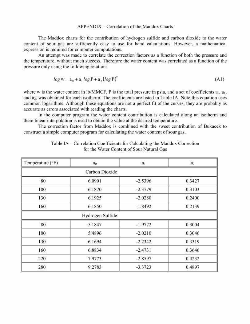
APPENDIX – Correlation of the Maddox Charts
The Maddox charts for the contribution of hydrogen sulfide and carbon dioxide to the watercontent of sour gas are sufficiently easy to use for hand calculations. However, a mathematicalexpression is required for computer computations.
An attempt was made to correlate the correction factors as a function of both the pressure andthe temperature, without much success. Therefore the water content was correlated as a function of thepressure only using the following relation:
( )2210 PaPaaw logloglog ++= (A1)
where w is the water content in lb/MMCF, P is the total pressure in psia, and a set of coefficients a0, a1,and a2, was obtained for each isotherm. The coefficients are listed in Table IA. Note this equation usescommon logarithms. Although these equations are not a perfect fit of the curves, they are probably asaccurate as errors associated with reading the charts.
In the computer program the water content contribution is calculated along an isotherm andthem linear interpolation is used to obtain the value at the desired temperature.
The correction factor from Maddox is combined with the sweet contribution of Bukacek toconstruct a simple computer program for calculating the water content of sour gas.
Table IA – Correlation Coefficients for Calculating the Maddox Correctionfor the Water Content of Sour Natural Gas