The Wealth of Ecosystems: Valuing Natural Capital in the Context of Ecosystem Based Management Seong Do Yun Postdoctoral Research Associate, Yale University | [email protected]Barbara Hutniczak Postdoctoral Researcher, NOAA | b[email protected]Eli P. Fenichel Assistant Professor, Yale University | [email protected]Joshua K. Abbott Associate Professor, Arizona State University | [email protected]Selected paper prepared for presentation at the 2016 Agricultural & Applied Economics Annual Meeting, Boston, Massachusetts, July 31-Auguest 2, 2016. Copyright 2016 by Seong Do Yun, Barbara Hutniczak, Eli P. Fenichel, and Joshua K. Abbott. All rights reserved. Readers may make verbatim copies of this document for non-commercial purposes by any means, provided that this copyright notice appears on all such copies.
Transcript
The Wealth of Ecosystems:
Valuing Natural Capital in the Context of Ecosystem Based Management
Seong Do Yun
Postdoctoral Research Associate, Yale University | [email protected]
where 𝒑 = (𝑝1(𝑺), 𝑝2(𝑺), ⋯ , 𝑝𝑁(𝑺)) is an array of accounting prices as a function of stocks, 𝑺.
Equation (7) is the CVH evaluated with the economic program 𝑥(𝑺), composed of the flow of
current benefits 𝑊(𝑺, 𝑥(𝑺)), and the value of increments to the stocks, ∑ 𝑝𝑖��𝑖𝑁𝑖=1 .3
Dividing 𝛿 on both sides, Equation (7) yields:
𝑉 =1
𝛿(𝑊(𝑺, 𝑥(𝑺)) + ∑ 𝑝𝑖��𝑖
𝑁𝑖=1 ). (8)
Differentiating Equation (8) with respect to 𝑠𝑖,
𝑝𝑖 =𝜕𝑉
𝜕𝑠𝑖=
1
𝛿(
𝜕𝑊
𝜕𝑠𝑖+ ∑ (
𝜕𝑝𝑗
𝜕𝑠𝑖��𝑗 + 𝑝𝑗
𝜕��𝑗
𝜕𝑠𝑖)𝑁
𝑗=1 )
3 Note that we manage a time autonomous case here. A generalization to non-autonomous case can be derived from
a similar way referring to Asheim (2000).
- 8 -
=1
𝛿(
𝜕𝑊
𝜕𝑠𝑖+ ∑ (
𝜕𝑝𝑗
𝜕𝑠𝑖��𝑗 + 𝑝𝑗
𝜕��𝑗
𝜕𝑠𝑖)𝑁
𝑖≠𝑗 + ��𝑖 + 𝑝𝑖𝜕��𝑖
𝜕𝑠𝑖) (9)
Rearranging Equation (9), we have the multiple stock version of the natural capital asset price
equation in Fenichel and Abbott (2014):
𝑝𝑖 =
𝜕𝑊
𝜕𝑠𝑖+��𝑖+∑ (
𝜕𝑝𝑗
𝜕𝑠𝑖��𝑗+𝑝𝑗
𝜕��𝑗
𝜕𝑠𝑖)𝑁
𝑖≠𝑗
𝛿−𝜕��𝑖𝜕𝑠𝑖
. (10)
Compared to the single stock version of price equation (Fenichel & Abbott, 2014; Fenichel et al.,
2016a; Fenichel et al., 2016b), Equation (10) has an additional term of cross stock effect,
∑ (𝜕𝑝𝑗
𝜕𝑠𝑖��𝑗 + 𝑝𝑗
𝜕��𝑗
𝜕𝑠𝑖)𝑁
𝑖≠𝑗 . Eq (10) enables us to develop a price function over all possible values of
the state variable on the current economic program in a single step. This leads the inclusive
wealth as the sum of product of shadow price and stock asset (Dasgupta, 2014) as:
𝐼𝑊 = ∑ 𝑝𝑖𝑠𝑖𝑁𝑖=1 , (11)
and Eq (10) enables us to track the changes in the natural capital assets contributions to inclusive
wealth through time.
From the differential equation form presented in Equation (8), 𝑉 and 𝑉𝑠𝑖= 𝑝𝑖, functional
approximations, the collocation method can be adopted to figure out 𝑝𝑖 numerically (Miranda &
Fackler, 2002). Following the V-approximation approach suggested in Abbott et al. (2016),
suppose we have the size 𝑀 of data for 𝑊 and ��𝑖 over the stock domain of the Chebyshev nodes,
𝑺(𝑡) = (𝑠1(𝑡), 𝑠2(𝑡), ⋯ , 𝑠𝑁(𝑡)) at a time point 𝑡, i.e., a 𝑀 × (𝑁 + 1 + 𝑁) data matrix.4 Then, we
define 𝜑𝑖 as the 𝑀 × (𝑑𝑖 + 1) basis matrix of 𝑑𝑖-th degree evaluated at the 𝑀 numbers of stock
combinations. Adopting the tensor product basis, the functional basis for real valued function is
4 It is not necessary for all data to be on Chebyshev nodes. For the convenience of description, we assume that the
data is collected (or generated) over the Chebyshev nodes used for Chebyshev polynomial approximation.
- 9 -
𝜑 = 𝜑𝑁 ⊗ 𝜑𝑁−1 ⊗ ⋯ ⊗ 𝜑1 where ⊗ is the Kronecker product. Due to the orthogonality and
multiple differentiability of the basis function, the Chebyshev polynomial can provide a
convenient way of approximation (Sauer, 2014). Returning back to Equation (8), let 𝑉(𝑺) =
𝜑(𝑺)𝛽 where 𝜑(𝑺) is the 𝑀𝑁 × ∏ (𝑑𝑖 + 1)𝑁𝑖=1 Chebyshev polynomial basis evaluated at the
stock combination 𝑺 and 𝛽 is an ∏ (𝑑𝑖 + 1)𝑁𝑖=1 × 1 unknown coefficients vector. From the
orthogonality of Chebyshev basis, 𝑝𝑖 =𝜕𝜑(𝑺)
𝜕𝑠𝑖𝛽 , Equation (8) becomes 𝛿𝜑(𝑺)𝛽 = 𝑊(𝑺) +
∑ 𝑑𝑖𝑎𝑔(��𝑖)𝜕𝜑(𝑺)
𝜕𝑠𝑖𝛽𝑁
𝑖=1 . If this is the exactly determined case (𝑀 = 𝑑𝑖), we can get the 𝛽 from:
𝛽 = (𝛿𝜑(𝑺) − ∑ 𝑑𝑖𝑎𝑔(��𝑖)𝜕𝜑(𝑺)
𝜕𝑠𝑖
𝑁𝑖=1 )
−1
𝑊(𝑺). (12.1)
In a case of over-determined (𝑀 ≥ 𝑑𝑖 for at least one 𝑖), we can derive 𝛽 from the least squares:
𝛽 = ((𝛿𝜑(𝑺) − ∑ 𝑑𝑖𝑎𝑔(��𝑖)𝜕𝜑(𝑺)
𝜕𝑠𝑖
𝑁
𝑖=1
)
𝑇
(𝛿𝜑(𝑺) − ∑ 𝑑𝑖𝑎𝑔(��𝑖)𝜕𝜑(𝑺)
𝜕𝑠𝑖
𝑁
𝑖=1
))
−1
× (𝛿𝜑(𝑺) − ∑ 𝑑𝑖𝑎𝑔(��𝑖)𝜕𝜑(𝑺)
𝜕𝑠𝑖
𝑁𝑖=1 )
𝑇
𝑊(𝑺) (12.2)
With a single stock version of Equation (10), Fenichel and Abbott (2014) suggest the ��-
approximation (by setting �� = 𝜑(𝑠)𝛽) and Fenichel et al. (2016) provide the 𝑝-approximation
(by letting 𝑝 = 𝜑(𝑠)𝛽 ). We, however, suspect that the computational burden for 𝑝- and �� -
approximation is greater than 𝑉 -approximation in the multi-dimensional case due to its
mathematical complexity and thus, a more high chance to have singularity and curse of
dimensionality. Due to its simplicity and relatively low computational burden, we adopt the 𝑉-
- 10 -
approximation for our analysis. We use the R-package ‘capN’5 (Yun et al., 2016) for the Baltic
Sea fishery analysis in the next two sections.
3. Baltic Sea Fishery: Multispecies Interaction Model
To validate the suggested capital theoretic framework in Equation (8) and its numerical
approximation, we adopt the multispecies interaction model of the Baltic Sea fishery from
Hutniczak (2015). The model in Hutniczak (2015) is a micro-macro link simulation model based
on individual vessel’s fishing behavior under the given regulations and the vessels’ aggregated
impacts on ecosystem. In the model, the fishing fleet consists of vessels that maximize vessel net
revenue subject to regulations, feasibility constraint (maximum days the vessel can spend at sea),
owned capital, production structure (in form of distance function estimated, based on available
log book data), and individual technical efficiency (derived from distance function estimates).
Effectively this is an agent-based model with a finite number of agents. Therefore, the
simulations generate the “data” (𝑊 and ��𝑖 over the interested combinations of stock domains) as
bumpy data surfaces rather than a smooth well-behaving global surface. Since it is rarely
possible to define an explicit simultaneous system of equations for ecosystems and EBM,6 a
simulation based model such as agent-based model could be more realistic and practical
alternative. To implement natural capital valuation, we first fit the generated data with
polynomial approximation and then, apply the suggested methods over the smoothly fit data of
5 “capN” provides the full functions for the Chebyshev polynomial approximations: the 𝑉-approximation for single
and multiple stocks, and the 𝑝- / ��-approximation for single stock cases. For the time of analysis (May, 2016), we
adopt the beta testing version 0.0.2 of “capN” package. 6 In here, we are not denying an existence of well-behaving system of equations. What we assume is the difficulty of
defining ex-ante equations of ecosystems and EBM.
- 11 -
𝑊 and ��𝑖. We believe that the smoothly fit curves are the intent of policy and the policy is not
purposefully producing lumpy behavioral and profit results.
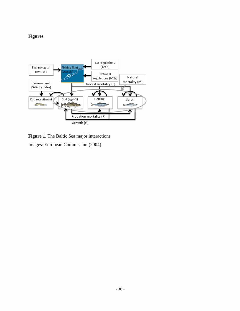
-- Figure 1 about here --
We investigate the central Baltic Sea as a case study, with its interacting fish community
dominated by three species: cod, herring and sprat (ICES, 2014). Cod plays an important
structuring role in this ecosystem as a predator of herring and sprat. By contrast, herring and
sprat, species belonging to the clupeid family, prey on cod eggs and impact cod growth, thus
creating a feedback loop that strongly ties these species together (Figure 1). We focus on Polish
fleet as one of the major fleets in the Baltic Sea.
3.1. Biological Process
The purpose of the multispecies interaction model is to realistically simulate changes
over time in stock sizes by taking the ecosystem structure into consideration. The biological
model includes three separate dynamically updating submodels for cod, herring and sprat linked
through predation. The predator species (cod) is a cause of predation mortality (P) whereas the
prey availability (herring and sprat) is influencing the predator’s consumption rates and its
growth (G). For simplicity, we assume that environmental factors are invariant such as the
sensitivity of cod to the salty water inflows from the North Sea.
The model suggests a sufficient overlap between species distribution range to model the
stocks as aggregated biomass, i.e. there are no localized populations for which spatial
distribution is mutually exclusive. The population dynamics in the base simulation model follow
the standard age-structured modeling methodology (Tahvonen, 2009). Disaggregating the adult
population into multiple age categories is assumed to better describe age-structured management
- 12 -
that imposes minimum mesh size and minimum landing sizes on the fishing fleets in the region;
therefore, welfare gain estimations are more precise (Quaas et al. 2013; Thøgersen & Hoff 2013).
The model is in discrete time in order to keep with biological reproduction (Finnoff & Tschirhart,
2003). The biological model is closely inspired by work of Heikinheimo (2011), whereas
includes several updating features based on recent development in the literature. The detail
models and parameters are described in the appendix.
3.2. Economic Program
The Baltic Sea fishery is an important industry in the coastal area of northern Poland and
relies on cod, herring and sprat as a main target species in about 79% in revenue terms (STECF,
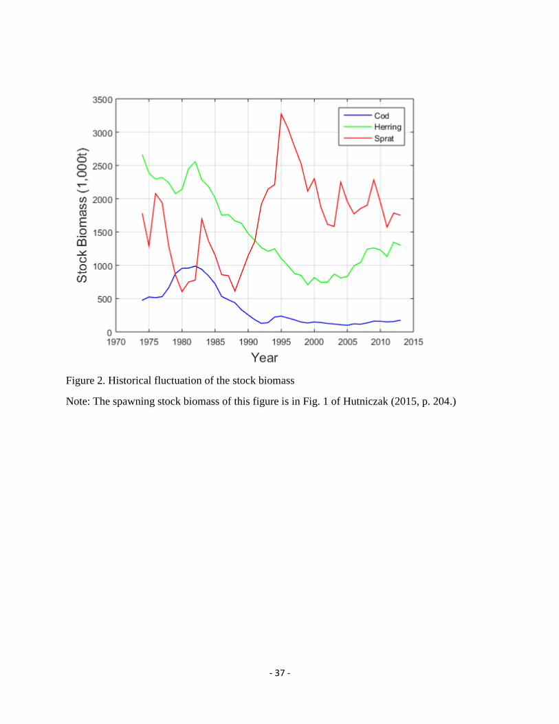
2015). The depletion of the Baltic Sea cod in the 1980s/1990s resulted in major regime shift
from predator- to prey-dominated ecosystem what makes it an interesting case study of human
impact on multispecies environment (Alheit et al., 2005; Hutniczak, 2015). Policy makers
responded to the shift with major changes in management (Alheit et al., 2005; Möllmann et al.,
2009) that can be evaluated in terms of altered value of this complex ecosystem (Figure 2).
-- Figure 2 about here --
The key regulatory tools are set annually total allowable catches (TAC) based on a single
species stock assessment and target fishing mortalities. The allocation between the European
Union (EU) members is based on the principle of relative stability, which implies that each
country receives a fixed share of each TAC (Churchill & Owen, 2010). The distribution of
national TAC between vessels or individual fishermen is the responsibility of individual
countries. Poland, a member of the EU since 2004, manages all three species by binding
- 13 -
individual allocations of TAC since 2014. The total allowance is divided among eligible units
according to the coefficient that depends on the vessel size.
3.3. Profit Maximization of Heterogeneous Vessels
The fishing fleet consists of vessels that optimize individual behavior subject to
regulations, owned capital, individual technical efficiency and current stock abundance. In this
context, the regulation of particular validity is the management plan allocating quotas for each
species affecting harvest now and in the future by impact on the stocks. Each unit employs effort
as input and attempts to achieve input efficiency. The individual vessel is considered here a
decision unit optimizing its own behavior over time that is simplified to assume profit
maximization.
Hutniczak (2015) adopts the multiproduct distance function with input oriented
specification (Shephard, 1970) as an effort requirement function. For individual vessel (𝑛 ∈ 𝑁),
fishing effort can be presented by the translog function:
ln(𝑒𝑛,𝑡) = ∑ 𝛼𝑖ln (ℎ𝑖,𝑛,𝑡)𝑖∈𝐼 + 𝛼𝑘ln (𝑘𝑛)
+ 1
2∑ ∑ 𝛼𝑖𝑖′ ln(ℎ𝑖,𝑛,𝑡) ln (ℎ𝑖′,𝑛,𝑡)𝑖′∈𝐼𝑖∈𝐼 +
1
2𝛼𝑘𝑘 ln(𝑘𝑛) ln (𝑘𝑛)
+ ∑ 𝛼𝑖𝑘 ln(ℎ𝑖,𝑛,𝑡) ln (𝑘𝑛)𝑖∈𝐼 + 𝑢𝑛 + 𝑢𝑡 + 𝑣𝑛,𝑡
= −𝑇𝐿(ℎ𝑛,𝑡, 𝑘𝑛) + 𝑢𝑛 + 𝑣𝑛,𝑡 , (13)
where 𝑒 is effort of fishing, 𝑖 ∈ 𝐼 = {𝑐, ℎ, 𝑠, 𝑜} is species for cod, herring, sprat and others,
𝑘 is vessel power, ℎ is harvested biomass, 𝑢𝑛 is individual vessel fixed effect, and 𝑣𝑛,𝑡 is
stochastic term. To reflect the direct and indirect effects of stock size on catch, we use harvest
transformed into partial fishing mortality (Pascoe et al, 2007) which in practical terms means that
harvest is divided by normalized stock variables derived as harvestable biomass (Hutniczak,
- 14 -
2015). In addition, all variables in Equation (13) are normalized by their means so that each
variable is a relative distance from its mean.7 All coefficients and technical efficiency were
estimated using individual fixed effects.
With the estimated coefficients of Equation (13), the profit maximization model of
heterogeneous vessel assumes the upper bound for effort denoted by 𝑒��8 that can be considered
a feasibility constraint. Thus, the harvest plan is adjusted from initial quota allocation according
to economic incentives (profitability criteria) and subject to effort restriction (feasibility criteria).
Assuming constant prices and adding a cost variable, the profit maximization problem is:
where 𝑥𝑗 is harvested quantity for species 𝑗 ∈ {𝑐, ℎ, 𝑠}, 𝑝𝑖 is price, subscript 𝑜 is all other species,
𝑐𝑣,𝑛 is variable cost per unit effort, and 𝑐𝑓 is fixed cost. Following Hutniczak (2015), we use
2008-2012 Polish fishery panel data for efficiency estimation and adopt the 2012 fleet structure
to implement the optimization of Equation (14) for simulation. The estimation procedure and the
parameters adopted in the model are described in Appendix B.
7 For example, ℎ =
𝑥
𝐵/ (
𝑥
𝐵)
where 𝑥 is quantity of harvest, 𝐵 is biomass index normalized at 2014, and (
𝑥
𝐵)
is the
mean of 𝑥
𝐵.
8 In the empirical analysis, two types of vessels (large vessels (longer than 12 meters) and small vessels (otherwise)
are adopted. For a large vessel, 𝑒�� is given as 160 days while 90 days does for a small vessel.
- 15 -
3.4. Simulation Data Generation
In section 2, we assume that the 𝑀 × (𝑁 + 1 + 𝑁) size of data set of 𝑊 and ��𝑖 from
various combinations of stocks are presented before implementing the suggested 𝑉 -
approximation of Equation (8) and Equation (12). In reality, however, such data are rarely
available. For our analysis, we perform the multispecies interaction model through the various
combinations of stocks to simulate 𝑊 and ��𝑖 using Poland fishing logbook data described in
Appendix B. In our case, the monetary terms of 𝑊 is the net revenue from harvesting cod,
herring and sprat, and the ��𝑖 is the change of stocks including fishing. Since available data covers
only short time period with limited combinations of biomass abundance, we rely on only 2012
data is available for figuring out all parameters of the biological process in Appendix A. We
simulate 411Polish fishing vessels (189 vessels longer than 12 m and 222 vessels shorter than 12
m) in 2012 as described in Appendix B. To represent the whole Baltic Sea fishing behavior and
use fixed multipliers,9 the ratio between the 411 and the Baltic Sea overall for each variable, to
the simulated variables.
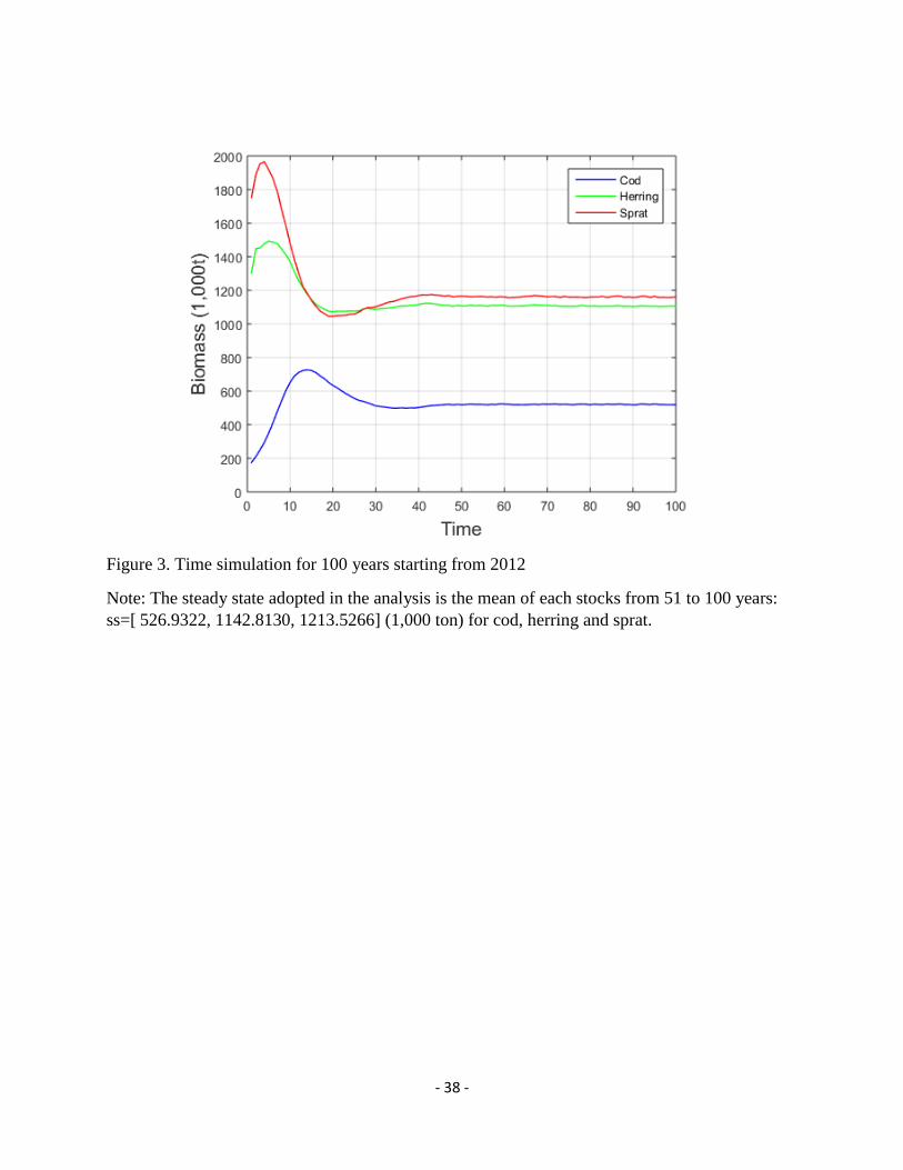
To determine approximation domains, we first investigate the stock changes for 100
years starting from the stocks of year 2012, [174.939, 1,302.509, 1,752.787] (1,000 tons) for cod,
herring and sprat (yearly stock fluctuations in Figure 2). Figure 3 presents the time dynamics of
100 years.10
-- Figure 3 about here --
About the 50th year and after, the stocks of three species converge to the stable level of stocks.
After confirming the stability of convergence with 150 years, we derived the steady state as the
9 These multipliers can be provided upon requests. 10 Wither more longer periods, up to 200 years, we confirmed that the 100 years are enough length to show the
steady state.
- 16 -
mean of stocks from 51st to 100th years; ss=[526.932, 1,142.813, 1,213.527] (1,000 tons) for cod,
herring and sprat.
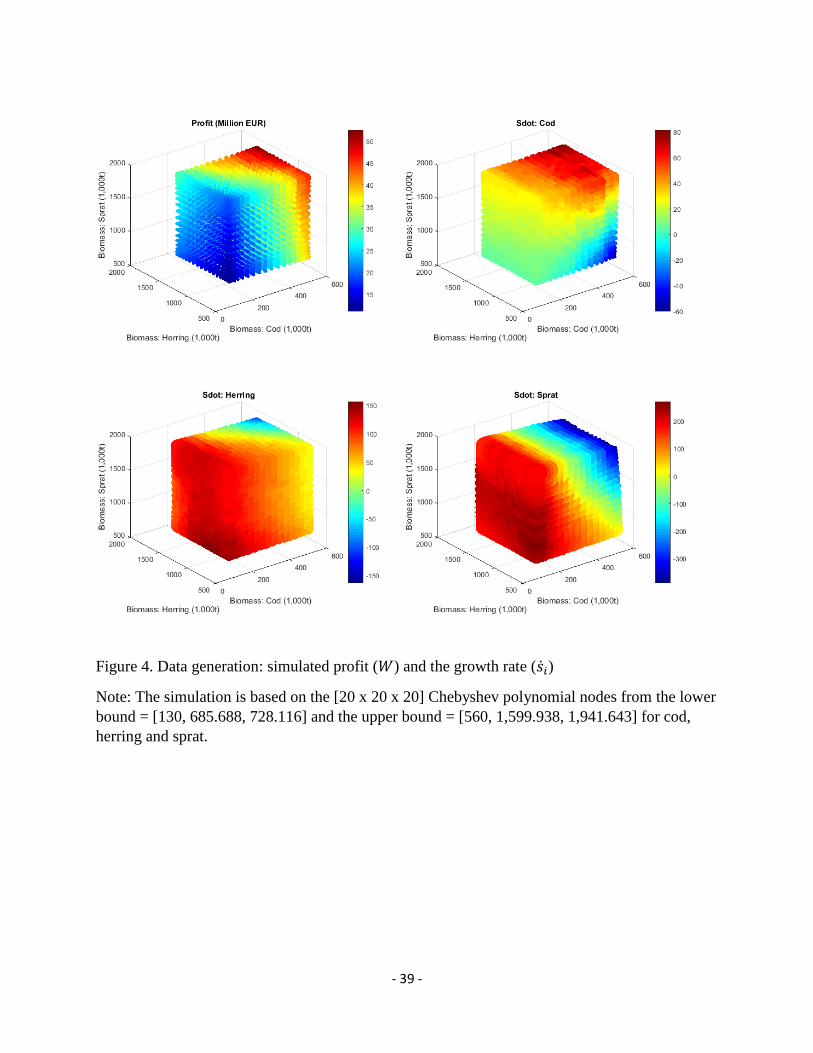
Based on the steady state and 2012 conditions, we set the simulation domain of the
multispecies interaction model as the lower bound = [130, 60% of the herring ss, 60% of the
sprat ss] and the upper bound = [560, 140% of the herring ss, 160% of the sprat ss]. It is
noteworthy that fishing is shut down when a species reach the moratorium level about [100, 580,
550] (1,000 tons) for cod, herring and sprat.11 The lower bound, therefore, is determined to avoid
the moratorium stock level safely, which creates discrete jumps in 𝑊 and ��𝑖 surfaces.12 Since the
2012 stock of cod (174,939 tons) and the recent historical stocks in Figure 2 were much lower
than the steady state level (526,932 tons), we set up 130,000 tons as the lower bound to make the
cod range more meaningful. On the other hand, due to its abundant historical stocks of sprat, we
set up the upper bounds as 140% and 160% of the steady state for herring and sprat. With the
given stock domains, we generate [20 x 20 x 20] Chebyshev polynomial nodes and simulate
profit (𝑊) and growth rate (��𝑖) shown in Figure 4.
-- Figure 4 about here --
As expected, more stocks for three species provide higher profits and more cod derives less
herring and sprat.
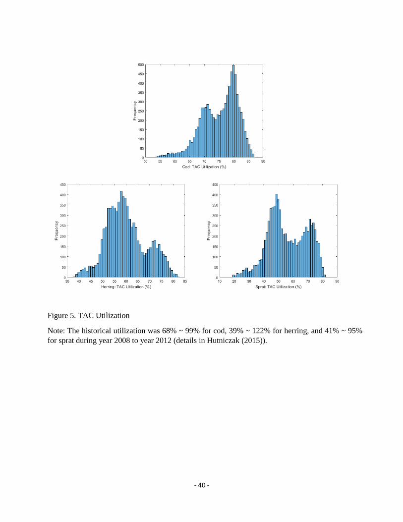
Since we simulate the Baltic Sea fishery from the fishing behavior of 411 Polish vessels,
the interpretation of simulation model needs to be considered carefully. For this purpose, we
calculate the TAC utilization (the percentage of harvest/TAC) from the simulation results.
Figure 5 show the histogram of utilizations from the 8,000 combinations of stock nodes.
11 Fishing is not allowed the stock levels below the moratorium level determined by the spawning stock biomass.
The presented bound of [100, 580, 550] (1,000 t) is the approximated numbers in stock biomass. 12 In numerical approximation, the classic Chebyshev polynomial approximation adopted in this paper is not
appropriate to simulate discontinuous or non-smooth functions (Mace, 2005).
- 17 -
-- Figure 5 about here --
In Hutniczak (2015), the historical TAC utilization was 68% ~ 99% for cod, 39% ~ 122% for
herring, and 41% ~ 95% for sprat during year 2008 to year 2012. Our simulation results in
Figure 5 suggests the TAC utilization from our model fall within realistic ranges.
4. Results and Discussion
We fit the data generated data in Figure 4 to a multivariate polynomial in order to smooth
the surfaces for 𝑊 and ��𝑖. This smoothing process is meant to provide reasonable derivatives
and enables us to abstract from the discrete nature of the fishing industry. As noted in Section 3,
the simulated data is likely to provide (sufficiently) well approximated values. It, however,
includes many bumpy spots that make it difficult to numerically handle the multivariate
approximation. Smooth functions bump up against the curse of dimensionality at higher
dimensions (CITE). Assuming well-behaving, but unknown, ex-post surfaces of 𝑊 and ��𝑖, we
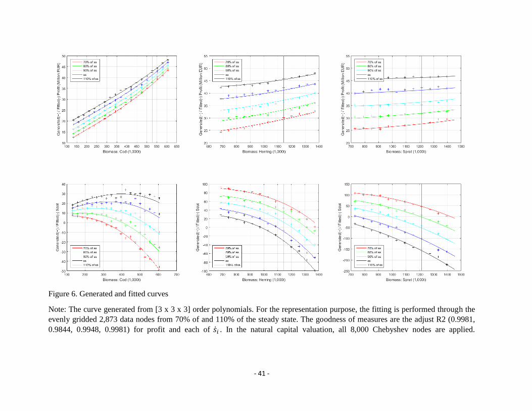
implement a multivariate polynomial least squares regression (Fig 6).
-- Figure 6 about here --
Instead of using [20 x 20 x 20] Chebyshev polynomial nodes described in Section 3.4, in Figure
6, we represent the fitted curves from [3 x 3 x 3] order polynomials from the evenly gridded
2,873 data nodes of 70% of and 110% of the steady state. All curves are highly well-fitted with
the adjusted R2 (0.9981, 0.9844, 0.9948, 0.9981) and the root mean squared errors (RMSE:
0.4052, 2.2090, 3.8796, 4.9706) for profit and each of ��𝑖. In the natural capital valuation process,
we fit the [20 x 20 x 20] Chebyshev polynomial nodes and the goodness of fit from [3 x 3 x 3]
- 18 -
order polynomials is that the adjusted R2 are (0.9976, 0.9918, 0.9947, 0.9974) and the RMSEs
are (0.4905, 2.3674, 5.0729, 8.2837).
Since this relatively low order of polynomials ([3 x 3 x 3]), we can achieve good enough
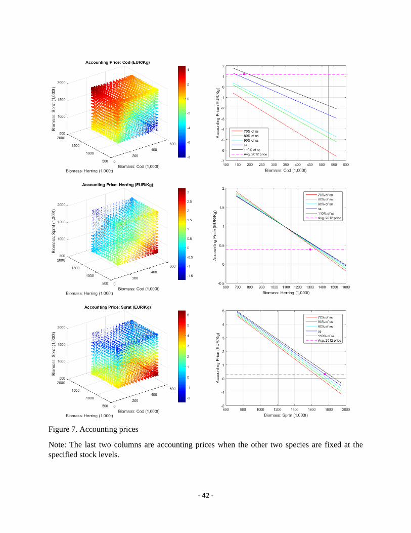
fit, we implement the Chebyshev polynomial approximations for Equation (12). With [3 x 3 x 3]
Chebyshev polynomial approximation, the accounting prices of three species are presented in
Figure 7.
-- Figure 7 about here --
Figure 7 approximates from the fitted data with the multivariate polynomials. The 8,000
generated data includes many bumpy spots over profit and the growth rate surfaces. To increase
the orders of polynomials to approximate these surfaces more smoothly, we can observe
oscillations. These oscillations are getting worse with higher orders (Gottlieb & Shu, 1997; Mace,
2005). In addition, it is noteworthy that the error convergent maximum orders for the fitted
curves in the first two columns are [3 x 3 x 3] due to the orders of fitted curves. If we increase
the orders higher than [3 x 3 x 3] by increasing the orders of fitted curves, the Chebyshev
polynomials provide higher error sizes and oscillations can be appeared. From our data, we
observe the Gibbs phenomenon from both cases.
From Figure 7, we configure three important accounting price behaviors. First, prices are
decreasing for all three species when holding the other two. As expected in general price curves,
our analysis achieves the negative slope of price curves, i.e, price decreases as quantity increases.
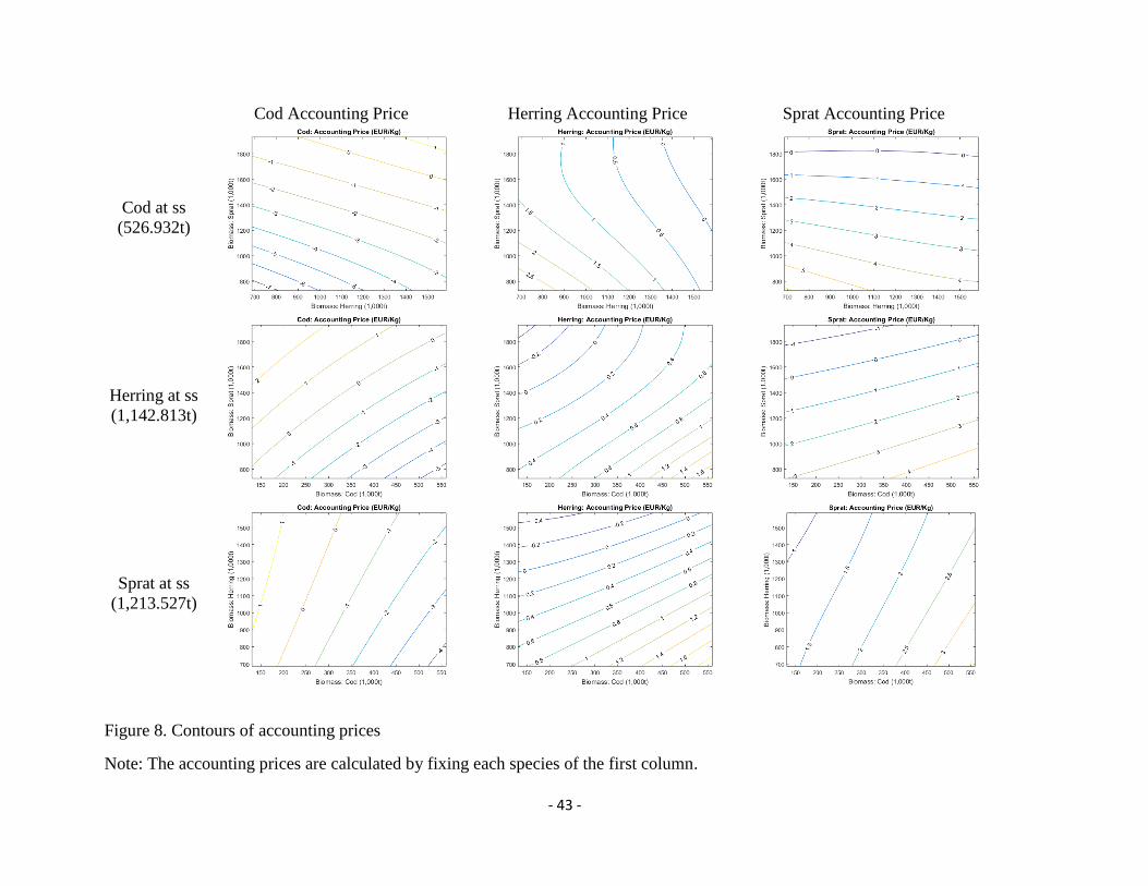
Second, cross-stock effects exist. At the first column of Figure 7, we can observe there are
nonlinear price changes along with stock combinations. In multiple stocks analysis, the price
curves include the cross-stock effects terms, ∑ (𝜕𝑝𝑗
𝜕𝑠𝑖��𝑗 + 𝑝𝑗
𝜕��𝑗
𝜕𝑠𝑖)𝑁
𝑖≠𝑗 in Equation (10), that creates
nonlinear substitution and complements among stocks. When holding one species stock, then we
- 19 -
can observe this nonlinear effect more clearly as shown in Figure 8. In Figure 8, each stock is
fixed at the steady state for the purpose of simplicity.
-- Figure 8 about here --
Lastly, the shadow price of cod is negative over large stock levels while the shadow price around
steady is close to the average of 2012 ex-vessel price. In the Baltic Sea ecosystems, herring and
sprat are prey and provide provision and regulating services. Cod is a multiple-use species
providing a direct provisioning service in the current management setting (Fenichel et al., 2010;
Horan & Bulte, 2004; Rondeau, 2001; Zivin et al, 2000). The multiple use species creates the
potential for ecosystem externalities (Crocker & Tschirhart, 1992), which is reflected in the
accounting price. Due to the possibility of non-convexities in our analysis, the accounting prices
in the results may reflect local dynamics rather than global dynamics.
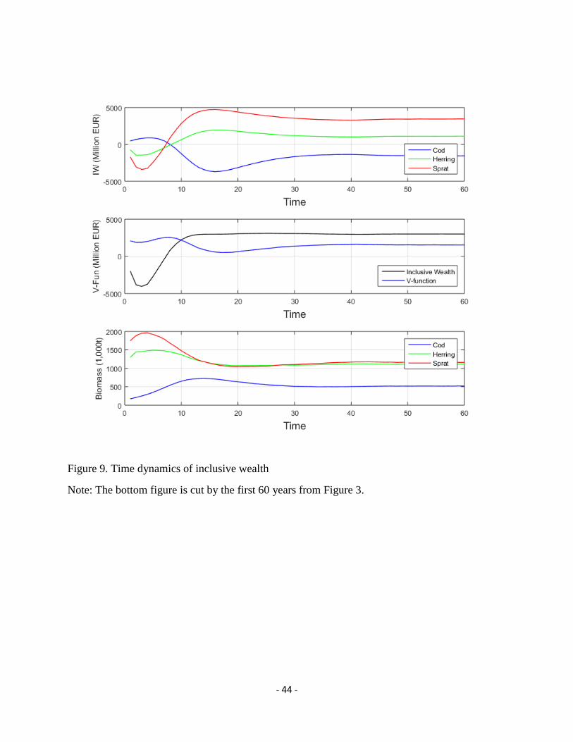
Following Equation (11), we calculate the inclusive wealth according to the time
dynamics in Figure 3 shown in Figure 9. Since there are steady state later 50th year, we present
only first 60 years dynamics of inclusive wealth.
-- Figure 9 about here --
From Figure 7 and 8, we can see that the accounting price of cod is positive with smaller cod but
larger herring and sprat stocks while the opposite happens for herring and sprat. The total
inclusive wealth are negative for the first several years. After that, the inclusive wealth becomes
positive due to positive accounting prices of herring and sprat. At the year 2012, herring and
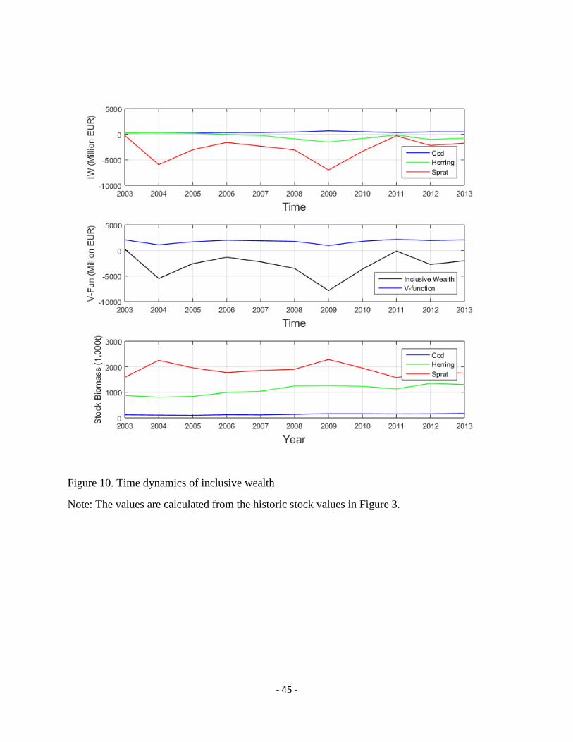
sprat stocks are relatively high but cod stock is a way below from the steady state. In Figure 10,
we calculate the inclusive wealth and estimated V-function value for the historic stocks of year
2003 to 2013.
-- Figure 10 about here --
- 20 -
5. Conclusion
This paper merges inclusive wealth accounting theory with ecosystem based management
(EBM) to numerally measure the value of ecosystem. Generalizing the FA method, we suggest
an approach to approximate realized shadow prices for multiple interacting stocks of biotic and
abiotic assets and liabilities that comprise ecosystems. We apply our approach to the Baltic Sea
ecosystem, focusing on the commercial fishing industry and three central fish species; cod,
herring and sprat. Our approach is relevant to economists interested in sustainability and green
accounting and to natural resource managers interested in EBM. Our contribution advances the
field towards an inclusive vision of wealth for measuring sustainability.
Since this draft is in a preliminary step of the whole research, we expect to include three
additional contents in near future. First, we will discuss more details on the results focusing on
interpretation of inclusive wealth and estimated V-function values. Second, we will derive deep
policy implication for the EBM of Baltic Sea and for general EBM policy. Last, additional
analysis to configure policy frictions, e.g. comparison between the current regime and tradable
permits system, could be discussed.
- 21 -
Appendix A: Biological Model
The biological model includes three separate submodels for cod, herring and sprat linked
through predation. The model parameters are derived based on the Report of the Baltic Fisheries
Assessment Working Group by the International Council for the Exploration of the Sea (ICES,
2014), unless noted otherwise. ICES provides the annual stock assessment of major Baltic Sea
species including a wide array of time-series indicators for species of our interest.
Each submodel includes 8 age classes, with the last category covering adults of age 8 and
higher. Let i, iϵ(c,h,s) denote the specific species that are included in the model: cod, herring and
sprat, respectively. Let a, aϵ[1,8] denote age class and t the time period. The modeled spawning
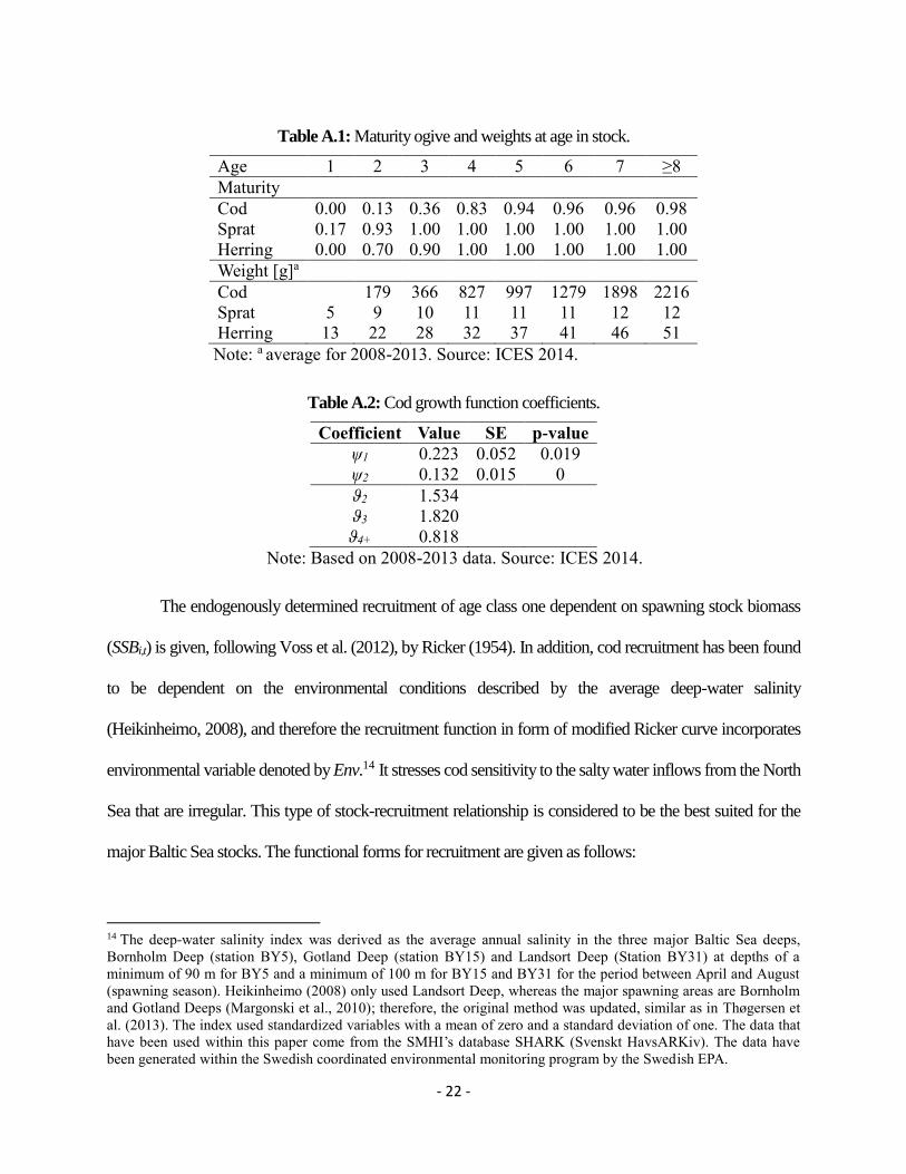
stock biomass (SSB, in thousands of tons) is derived from the latest estimation of maturity ogive
(ζi,a) and weights at age in stock (wi,a) available in table A.1.:
𝑆𝑆𝐵𝑖 = ∑ 휁𝑖,𝑎𝑤𝑖,𝑎8𝑎=1 𝑥𝑖,𝑎. (A.1)
Following the Benchmark Workshop on Baltic Multispecies Assessment (ICES WKBALT, 2013)
approach, weight of adult cod is found significantly impacted by the amount of prey available,
whereas weight of recruitment is based on weight of cod in spawning stock (wc SSB). This is
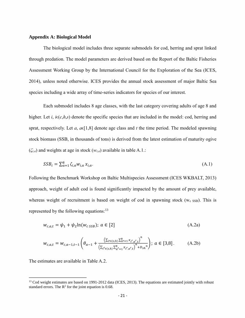
represented by the following equations:13
𝑤𝑐,𝑎,𝑡 = 𝜓1 + 𝜓2ln (𝑤𝑐 𝑆𝑆𝐵); 𝑎 ∈ [2] (A.2a)
𝑤𝑐,𝑎,𝑡 = 𝑤𝑐,𝑎−1,𝑡−1 (𝜃𝑎−1 +(∑ ∑ 𝑥
𝑖′,𝑎′,𝑡8𝑎′=1𝑖′∈(𝑠,ℎ) )
𝑛
(∑ ∑ 𝑥𝑖′,𝑎′,𝑡8𝑎′=1𝑖′∈(𝑠,ℎ) )
𝑛+𝐷𝑠ℎ
𝑛) ; 𝑎 ∈ [3,8] . (A.2b)
The estimates are available in Table A.2.
13 Cod weight estimates are based on 1991-2012 data (ICES, 2013). The equations are estimated jointly with robust
standard errors. The R2 for the joint equation is 0.68.
- 22 -
Table A.1: Maturity ogive and weights at age in stock.
Age 1 2 3 4 5 6 7 ≥8
Maturity
Cod 0.00 0.13 0.36 0.83 0.94 0.96 0.96 0.98
Sprat 0.17 0.93 1.00 1.00 1.00 1.00 1.00 1.00
Herring 0.00 0.70 0.90 1.00 1.00 1.00 1.00 1.00
Weight [g]a
Cod 179 366 827 997 1279 1898 2216
Sprat 5 9 10 11 11 11 12 12
Herring 13 22 28 32 37 41 46 51
Note: a average for 2008-2013. Source: ICES 2014.
Table A.2: Cod growth function coefficients.
Coefficient Value SE p-value
ψ1 0.223 0.052 0.019
ψ2 0.132 0.015 0
ϑ2 1.534
ϑ3 1.820
ϑ4+ 0.818
Note: Based on 2008-2013 data. Source: ICES 2014.
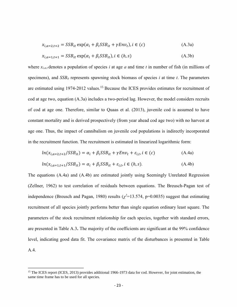
The endogenously determined recruitment of age class one dependent on spawning stock biomass
(SSBi,t) is given, following Voss et al. (2012), by Ricker (1954). In addition, cod recruitment has been found
to be dependent on the environmental conditions described by the average deep-water salinity
(Heikinheimo, 2008), and therefore the recruitment function in form of modified Ricker curve incorporates
environmental variable denoted by Env.14 It stresses cod sensitivity to the salty water inflows from the North
Sea that are irregular. This type of stock-recruitment relationship is considered to be the best suited for the
major Baltic Sea stocks. The functional forms for recruitment are given as follows:
14 The deep-water salinity index was derived as the average annual salinity in the three major Baltic Sea deeps,
Bornholm Deep (station BY5), Gotland Deep (station BY15) and Landsort Deep (Station BY31) at depths of a
minimum of 90 m for BY5 and a minimum of 100 m for BY15 and BY31 for the period between April and August
(spawning season). Heikinheimo (2008) only used Landsort Deep, whereas the major spawning areas are Bornholm
and Gotland Deeps (Margonski et al., 2010); therefore, the original method was updated, similar as in Thøgersen et
al. (2013). The index used standardized variables with a mean of zero and a standard deviation of one. The data that
have been used within this paper come from the SMHI’s database SHARK (Svenskt HavsARKiv). The data have
been generated within the Swedish coordinated environmental monitoring program by the Swedish EPA.
Note: based on 2008-2013 data (ICES, 2014); Standard errors in brackets; a no harvest activity in
16 The surprisingly decreasing selectivity coefficient for cod at age categories starting from 6 may be explained by
old specimens being rare and the potential to exhibit different behavior patterns.
- 27 -
the given age category. Source: ICES, 2014.
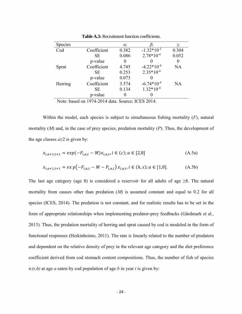
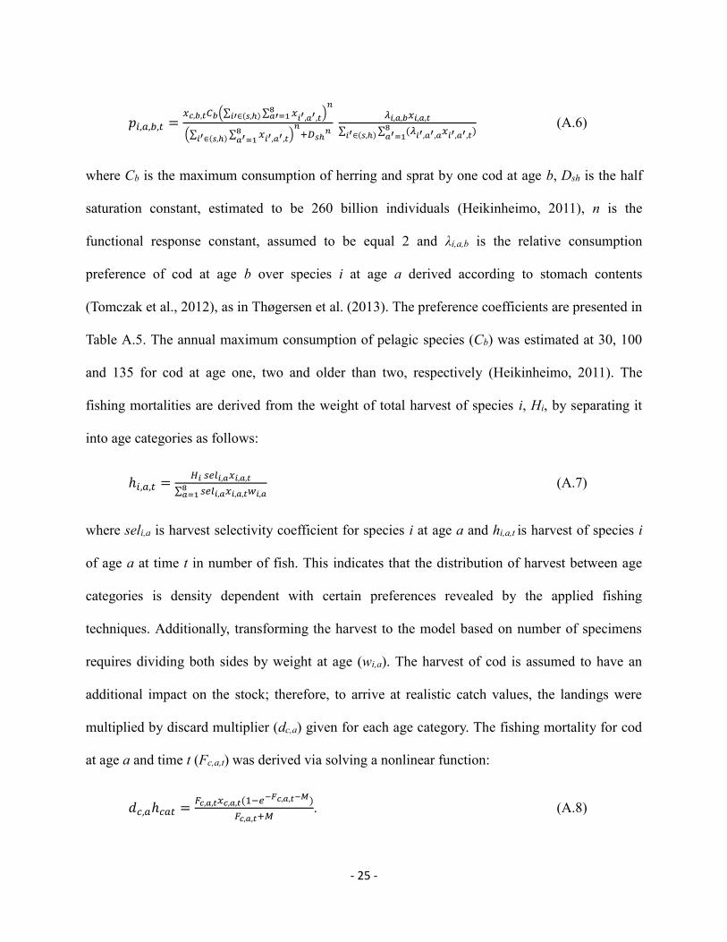
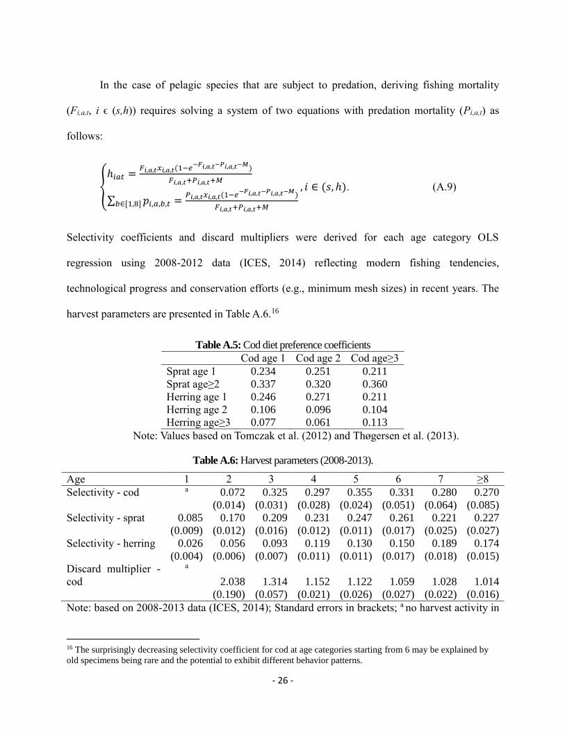
Fish stocks described by the multispecies interaction model are also subject to
commercial harvest by the existing fleet (limited entry regulations). The maximum harvest of
cod, herring and sprat within the model is given as a single species TAC. The total catch
allowance is derived according to harvest control rules (HCRs) based on target fishing mortality
that follow regulations currently in place (Council Regulation (EC) No 1098/2007 for cod, CFP
for herring and sprat). Under the current cod management plan, the goal in terms of F is equal to
0.3 for cod ages between 4 and 7. The HCR for pelagic species follows the single species
maximum sustainable yield (MSY) with F values 0.29 for sprat (age 3-5) and 0.18 for herring
(age 3-6). The TAC is set annually and therefore the management in place can be considered
adaptive (Walters and Hilborn, 1978), as total catch is adjusted every year to meet the
management plan target as close as possible. The risk of overfishing is reduced by setting limit
reference points under which harvest is prohibited. The limit reference points are set by ICES
and refer to the minimum spawning biomass, which permits a long-term sustainable exploitation
of the stock. The levels below are considered to be possibly dangerous for the capacity of self-
renewal of the stock (Caddy and Mahon, 1995). Those values are, in 1000 tones, 63 for cod, 430
for herring and 410 for sprat (ICES 2014).
Appendix B. Profit Maximization Process
Detailed data on harvest by the Polish fishing fleet is available through the Polish
Fisheries Monitoring Centre in Gdynia, which is a branch of the Fisheries Department under the
Ministry of Agriculture and Rural Development in Warsaw. It is confidential data originating
from the vessel logbooks, and it contains detailed harvest volumes (fresh weight) of each species
for each fishing trip performed in the Baltic Sea in the period 2008-2012 together with vessel
- 28 -
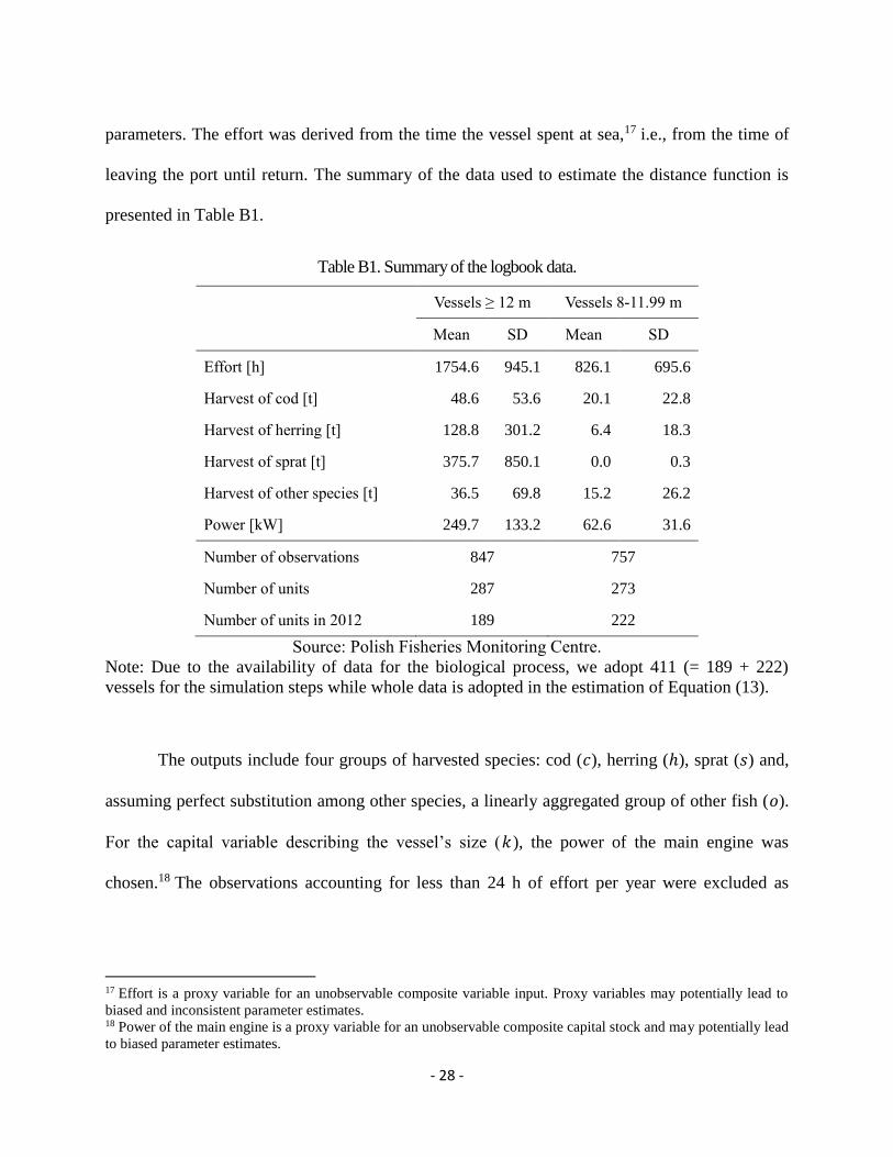
parameters. The effort was derived from the time the vessel spent at sea,17 i.e., from the time of
leaving the port until return. The summary of the data used to estimate the distance function is
presented in Table B1.
Table B1. Summary of the logbook data.
Vessels ≥ 12 m Vessels 8-11.99 m
Mean SD Mean SD
Effort [h] 1754.6 945.1 826.1 695.6
Harvest of cod [t] 48.6 53.6 20.1 22.8
Harvest of herring [t] 128.8 301.2 6.4 18.3
Harvest of sprat [t] 375.7 850.1 0.0 0.3
Harvest of other species [t] 36.5 69.8 15.2 26.2
Power [kW] 249.7 133.2 62.6 31.6
Number of observations 847 757
Number of units 287 273
Number of units in 2012 189 222
Source: Polish Fisheries Monitoring Centre.
Note: Due to the availability of data for the biological process, we adopt 411 (= 189 + 222)
vessels for the simulation steps while whole data is adopted in the estimation of Equation (13).
The outputs include four groups of harvested species: cod (𝑐), herring (ℎ), sprat (𝑠) and,
assuming perfect substitution among other species, a linearly aggregated group of other fish (𝑜).
For the capital variable describing the vessel’s size (𝑘), the power of the main engine was
chosen.18 The observations accounting for less than 24 h of effort per year were excluded as
17 Effort is a proxy variable for an unobservable composite variable input. Proxy variables may potentially lead to
biased and inconsistent parameter estimates. 18 Power of the main engine is a proxy variable for an unobservable composite capital stock and may potentially lead
to biased parameter estimates.
- 29 -
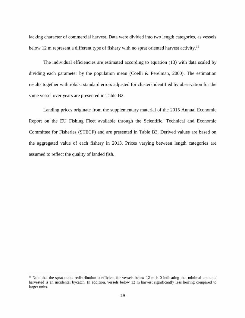
lacking character of commercial harvest. Data were divided into two length categories, as vessels
below 12 m represent a different type of fishery with no sprat oriented harvest activity.19
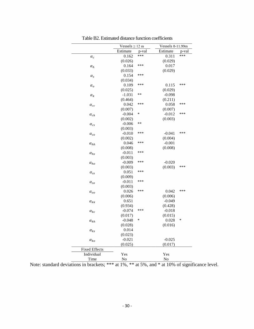
The individual efficiencies are estimated according to equation (13) with data scaled by
dividing each parameter by the population mean (Coelli & Perelman, 2000). The estimation
results together with robust standard errors adjusted for clusters identified by observation for the
same vessel over years are presented in Table B2.
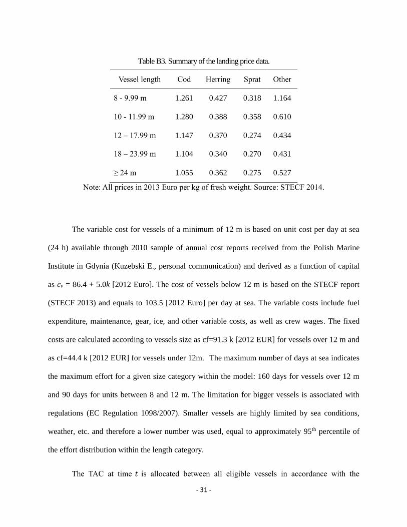
Landing prices originate from the supplementary material of the 2015 Annual Economic
Report on the EU Fishing Fleet available through the Scientific, Technical and Economic
Committee for Fisheries (STECF) and are presented in Table B3. Derived values are based on
the aggregated value of each fishery in 2013. Prices varying between length categories are
assumed to reflect the quality of landed fish.
19 Note that the sprat quota redistribution coefficient for vessels below 12 m is 0 indicating that minimal amounts
harvested is an incidental bycatch. In addition, vessels below 12 m harvest significantly less herring compared to
larger units.
- 30 -
Table B2. Estimated distance function coefficients
Vessels ≥ 12 m Vessels 8-11.99m
Estimate p-val
Estimate p-val
𝛼𝑐 0.162 ***
0.311 ***
(0.026)
(0.029)
𝛼ℎ 0.164 ***
0.017
(0.033)
(0.029)
𝛼𝑠 0.154 ***
(0.034)
𝛼𝑜 0.109 ***
0.115 ***
(0.025)
(0.029)
𝛼𝑘 -1.031 **
-0.098
(0.464)
(0.211)
𝛼𝑐𝑐 0.042 ***
0.058 ***
(0.007)
(0.007)
𝛼𝑐ℎ -0.004 *
-0.012 ***
(0.002)
(0.003)
𝛼𝑐𝑠 -0.006 **
(0.003)
𝛼𝑐𝑜 -0.010 ***
-0.041 ***
(0.002)
(0.004)
𝛼ℎℎ 0.046 ***
-0.001
(0.008)
(0.008)
𝛼ℎ𝑠 -0.011 ***
(0.003)
𝛼ℎ𝑜 -0.009 ***
-0.020
(0.003)
(0.003) ***
𝛼𝑠𝑠 0.051 ***
(0.009)
𝛼𝑠𝑜 -0.011 ***
(0.003)
𝛼𝑜𝑜 0.026 ***
0.042 ***
(0.006)
(0.006)
𝛼𝑘𝑘 0.651
-0.049
(0.934)
(0.428)
𝛼𝑘𝑐 -0.074 ***
-0.018
(0.017)
(0.015)
𝛼𝑘ℎ -0.048 *
0.028 *
(0.028)
(0.016)
𝛼𝑘𝑠 0.014
(0.023)
𝛼𝑘𝑜 -0.021
-0.025
(0.025)
(0.017)
Fixed Effects
Individual Yes Yes
Time No No
Note: standard deviations in brackets; *** at 1%, ** at 5%, and * at 10% of significance level.
- 31 -
Table B3. Summary of the landing price data.
Vessel length Cod Herring Sprat Other
8 - 9.99 m 1.261 0.427 0.318 1.164
10 - 11.99 m 1.280 0.388 0.358 0.610
12 – 17.99 m 1.147 0.370 0.274 0.434
18 – 23.99 m 1.104 0.340 0.270 0.431
≥ 24 m 1.055 0.362 0.275 0.527
Note: All prices in 2013 Euro per kg of fresh weight. Source: STECF 2014.
The variable cost for vessels of a minimum of 12 m is based on unit cost per day at sea
(24 h) available through 2010 sample of annual cost reports received from the Polish Marine
Institute in Gdynia (Kuzebski E., personal communication) and derived as a function of capital
as cv = 86.4 + 5.0k [2012 Euro]. The cost of vessels below 12 m is based on the STECF report
(STECF 2013) and equals to 103.5 [2012 Euro] per day at sea. The variable costs include fuel
expenditure, maintenance, gear, ice, and other variable costs, as well as crew wages. The fixed
costs are calculated according to vessels size as cf=91.3 k [2012 EUR] for vessels over 12 m and
as cf=44.4 k [2012 EUR] for vessels under 12m. The maximum number of days at sea indicates
the maximum effort for a given size category within the model: 160 days for vessels over 12 m
and 90 days for units between 8 and 12 m. The limitation for bigger vessels is associated with
regulations (EC Regulation 1098/2007). Smaller vessels are highly limited by sea conditions,
weather, etc. and therefore a lower number was used, equal to approximately 95th percentile of
the effort distribution within the length category.
The TAC at time 𝑡 is allocated between all eligible vessels in accordance with the
- 32 -
redistribution system currently in use (regulation 282/1653 from December 23, 2011 [in Polish]).
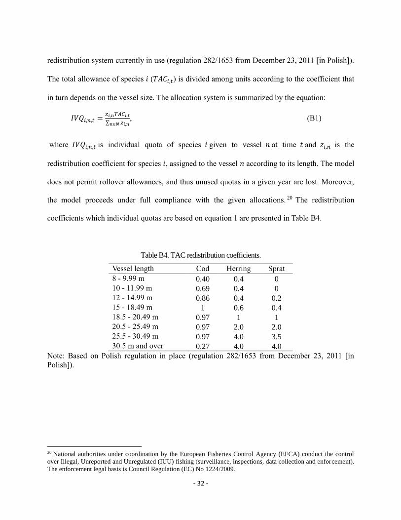
The total allowance of species 𝑖 (𝑇𝐴𝐶𝑖,𝑡) is divided among units according to the coefficient that
in turn depends on the vessel size. The allocation system is summarized by the equation:
𝐼𝑉𝑄𝑖,𝑛,𝑡 =𝑧𝑖,𝑛𝑇𝐴𝐶𝑖,𝑡
∑ 𝑧𝑖,𝑛𝑛∈𝑁, (B1)
where 𝐼𝑉𝑄𝑖,𝑛,𝑡 is individual quota of species 𝑖 given to vessel 𝑛 at time 𝑡 and 𝑧𝑖,𝑛 is the
redistribution coefficient for species 𝑖, assigned to the vessel 𝑛 according to its length. The model
does not permit rollover allowances, and thus unused quotas in a given year are lost. Moreover,
the model proceeds under full compliance with the given allocations. 20 The redistribution
coefficients which individual quotas are based on equation 1 are presented in Table B4.
Table B4. TAC redistribution coefficients.
Vessel length Cod Herring Sprat
8 - 9.99 m 0.40 0.4 0
10 - 11.99 m 0.69 0.4 0
12 - 14.99 m 0.86 0.4 0.2
15 - 18.49 m 1 0.6 0.4
18.5 - 20.49 m 0.97 1 1
20.5 - 25.49 m 0.97 2.0 2.0
25.5 - 30.49 m 0.97 4.0 3.5
30.5 m and over 0.27 4.0 4.0
Note: Based on Polish regulation in place (regulation 282/1653 from December 23, 2011 [in
Polish]).
20 National authorities under coordination by the European Fisheries Control Agency (EFCA) conduct the control
over Illegal, Unreported and Unregulated (IUU) fishing (surveillance, inspections, data collection and enforcement).
The enforcement legal basis is Council Regulation (EC) No 1224/2009.
- 33 -
References
Abbott, J. K., E. P. Fenichel, and S. D. Yun, (2016), “Inclusive Wealth and Sustainability in
Coupled Ecological-Economic Systems,” Working paper in Arizona State University and
Yale Univeristy.
Alheit, J., C. Möllmann, J. Dutz, G. Kornilovs, P. Loewe, V. Mohrholz, and N. Wasmund,
“Synchronous Ecological Regime Shifts in the Central Baltic and the North Sea in the
late 1980s,” ICES Journal of Marine Science, 62:1205-1215.
Arrow, K. J., P. Dagupta, and K. G. Mäler, 2003, “Evaluating Projects and Assessing Sustainable
Development in Imperfect Economies,” Environmental and Resource Economics,
26:647-685.
Asheim, G. B., 2000, “Green National Accounting: Why and How?”, Environmental and
Resource Economics, 5:25-48.
Barbier, E. B, 2011, Capitalizing on Nature. New York: Cambridge Unviersity Press.
Barbier, E. B., 2013, “Wealth Accounting, Ecological Capital and Ecosystem Services,”
Environmental and Development Economics, 18(2):133-161.
Caddy, J. F., and R. Mahon, 1995, Reference Points for Fishery Management, Rome: Food and
Agriculture Organization of the United Nations.
Christensen, N. L., A. M. Bartusak, J. H. Brown, S. Carptenter, C. D’Antonio, R. Francis, J.
Franklin, J. A. MacMahon, R. F. Noss, D. J. Parsons, C. H. Peterson, M. G. Turner, and
R. G. Woomansee, 1996, “The Report of the Ecological Society of America Committee
on the Scientific Basis for Ecosystem Management,” Ecological applications, 6:665-691.
Churchill, R. and D. Owen, 2010, The EC Common Fisheries Policy, Oxford: University Press.
Crocker, T. D., and J. Tschirhart, 1992, “Ecosystems, Externalities, and Economies,”
Environmental and Resource Economics, 2:551-567.
Dasgupta, P., 2014, “Measuring the Wealth of Nations,” Annual Review of Resource Economics,
6:17-31.
Dasgupta, P., and K. G. Mäler, 2000, “Net National Product, Wealth, and Social Well-being,”
Environmental and Development Economics, 5:69-93.
Dasgupta, P., K. G. Mäler, and S. Barrett, 1999, “Intergenerational Equity, Social Discount Rates
and Global Warming,” In Discounting and Intergenerational Equity, (ed.) Paul Portney
and John Weyant, Washington D.C.: Resources for the Future.
EC (European Commission), 2004, Fish of the Baltic Sea, Luxembourg: Office for Official
Publications of the European Communities.
EC (European Commission), 2013, Retrospective Evaluation of Permanent and Temporary
Cessation Measures in the EFF, Brussels: European Commission.
Fenichel, E. P., and J. K. Abbott, 2014, “Natural Capital: From Metaphor to Measurement,”
Journal of the Association of Environmental and Resource Economists, 1(1):1-27.
- 34 -
Fenichel, E. P., J. K. Abbot, J. Bayham, W. Boone, E. M. K. Haacker, and L. Pfeiffer, 2016a,
“Measuring the Value of Groundwater and Other Forms of Natural Capital,” Proceedings
of the National Academy of Science (PNAS), 113:2382-2387.
Fenichel, E. P., R. D. Horan, and J. R. Bence, 2010, “Indirect Management of Invasive Species
with Bio-control: A Bioeconomic Model of Salmon and Alewife in Lake Michigan,”
Resource and Energy Economics, 32:500-518.
Fenichel, E. P., S. A. Levin, B. McCay, K. Martin, J. K. Abbott, and M. L. Pinsky, 2016b,
“Wealth Reallocation and Sustainability under Climate Change,” Nature Climate Change,
6.3:237-244.
Finnoff, D. and J. Tschirhart, 2003, “Protecting an Endangered Species While Harvesting Its
Prey in a General Equilibrium Ecosystem Model,” Land Economics, 79(2):160-180.
Fisher, I., 1906, The Nature of Capital and Income, Norwood, MA: Norwood Press.
Gottlieb, D., and C. W. Shu, 1997, “Con the Gibbs Phenomenon and Its Resolution,” Society for
Industrial and Applied Mathematics (SIAM) Review, 39(4):644-668.
Heikinheimo, O., 2011, “Interactions between Cod, Herring and Sprat in the Changing
Environment of the Baltic Sea,” Ecological Modeling, 222:1731-1742.
Horan, R. D., and E. H. Bulte, 2004, “Optimal and Open Access Harvesting of Multi-use Species
in a Second Best World,” Environmental and Resource Economics, 28:251-272.
Hamilton, K., J. M. Hartwick, 2014, “Wealth and Sustainability,” Oxford Review of Economic
Policy, 30:170-187.
Hutniczak, B., 2015, “Modeling Heterogeneous Fleet in an Ecosystem Based Management
Context,” Ecological Economics, 120:203-214.
ICES (International Council for the Exploration of the Sea), 2013, Report of the Benchmark
Workshop on Baltic Multispecies Assessment (WKBALT), Copenhagen: ICES.
ICES (International Council for the Exploration of the Sea), 2014, Report of the Baltic Fisheries
Assessment Working Group (WGBFAS), Copenhagen: ICES.
Jorgenson, D. W., 1963, “Capital Theory and Investment Behavior,” American Economic Review,
53(2):247-259.
Mace, R. L., 2005, “Reduction of the Gibbs Phenomenon via Interpolation Using Chebyshev
Polynomials, Filtering and Chebyshev-Pade’ Approximations,” Theses, Dissertations and
Capstones, Paper 717.
Miranda, M. J., and P. L. Fackler, 2002, Applied Computational Economics and Finance,
Cambridge: The MIT press.
Möllmann, C. R. Diekmann, B. Müller-Karulis, G. Kornilovs, M. Plikshs, and P. Axe, 2008,
“Reorganization of a Large Marine Ecosystem due to Atmospheric and Anthropogenic
Pressure: A Discontinuous Regime Shift in the Central Baltic Sea,” Global Change
Biology, 15:1377-1393
Pascoe, S., P. Koundouri, and T. Bjørndal, 2007, “Estimating Targeting Ability in Multi-species
Fihseries: A Primal Multi-output distance function approach,” Land Economics,
83(3):382-397.
- 35 -
Pikitch, E. K., C. Santora, E. A. Babcock, A. Bakun, R. Bonfil, D. O. Conover, P. Dayton, P.
Doukakis, D. Fluharty, B. Heneman, E. E. Houde, J. Link, P. A. Livingston, M. Mangel,
M. K. AcAllister, J. Pope, K. J. Sainsbury, “Ecosystem-Based Management, Science,
300:2003-2003.
Pitcher, J. J., D. Kalikoski, K. Short, D. Varkeya, G. Pramod, 2009, “An Evaluation of Progress
in Implementing Ecosystem-based Management of Fisheries in 33 Countries,” Marine
Policy, 33:223-232.
Quaas, M. F., T. Requate, K. Ruckes, A. Skonhoft, N. Vestergaard, and R. Voss, 2013,
“Incentives for Optimal Management of Age-structured Fish Populations,” Resource and
Energy Economics, 35(2):113-134.
Rondeau, D., 2001, “Along the Way Back from the Brink,” Journal of Environmental Economics