+ All Categories
Home > Documents > Theoretical and Experimental Studies on the Minimum Size 2 ... · Theoretical and Experimental...

Theoretical and Experimental Studies on the Minimum Size 2 ... · Theoretical and Experimental...

Date post: 24-Mar-2020
Category:
Upload: others
View: 14 times
Download: 0 times
Share this document with a friend
150
Theoretical and Experimental Studies on the Minimum Size 2-edge-connected Spanning Subgraph Problem Yu Sun Thesis submitted to the Faculty of Graduate and Postdoctoral Studies in partial fulfillment of the requirements for a master degree in COMPUTER SCIENCE Ottawa-Carleton Institute for Computer Science University of Ottawa c Yu Sun, Ottawa, Canada, 2013
Transcript

Theoretical and Experimental Studies on

the Minimum Size 2-edge-connected

Spanning Subgraph Problem

Yu Sun

Thesis submitted to the

Faculty of Graduate and Postdoctoral Studies

in partial fulfillment of the requirements

for a master degree in

COMPUTER SCIENCE

Ottawa-Carleton Institute for Computer Science

University of Ottawa

c© Yu Sun, Ottawa, Canada, 2013

Abstract

A graph is said to be 2-edge-connected if it remains connected after the deletion of any

single edge. Given an unweighted bridgeless graph G with n vertices, the minimum

size 2-edge-connected spanning subgraph problem (2EC) is that of finding a 2-edge-

connected spanning subgraph of G with the minimum number of edges. This problem

has important applications in the design of survivable networks. However, because

the problem is NP-hard, it is unlikely that efficient methods exist for solving it. Thus

efficient methods that find solutions that are provably close to optimal are sought.

In this thesis, an approximation algorithm is presented for 2EC on bridgeless cubic

graphs which guarantees to be within 54

of the optimal solution value, improving on the

previous best proven approximation guarantee of 54+ǫ for this problem. We also focus

on the linear programming (LP) relaxation of 2EC, which provides important lower

bounds for 2EC in useful solution techniques like branch and bound. The “goodness”

of this lower bound is measured by the integrality gap of the LP relaxation for 2EC,

denoted by α2EC. Through a computational study, we find the exact value of α2EC

for graphs with small n. Moreover, a significant improvement is found for the lower

bound on the value of α2EC for bridgeless subcubic graphs, which improves the known

best lower bound on α2EC from 98

to 87.

i

Acknowledgments

This thesis would not have been possible without my supervisor, Dr. Sylvia Boyd,

and I greatly appreciate her incredible support, which can only be described as opti-

mal. She is the person who introduced me to the fascinating field of Combinatorial

Optimization and this brilliant problem, who guided and encouraged me all the way

through the research process, and who spent a huge amount of time reading my the-

sis drafts and giving me valuable suggestions. I could not thank her enough for her

dedicated guidance and generous financial support. It is a great pleasure to know her

and work with her for her cheerfulness, agreeableness and enthusiasm.

Many thanks to Dr. Liang Ji, Patrick Niesink, Fu Yao, Tracy Ng, Dr. Maryam

Haghighi, Dr. Amy Cameron, Mei Bin, Sheila Williams, Dr. Tet Yeap, Dr. Xiao

Sun, Yamin Jin, Yalu Su, and Yingjie Li for their advice, suggestions, help and moral

support. I also would like to thank all my professors who enlightened and guided me

in the field of Computer Science, especially Dr. Ji Qijin, Dr. Fan Jianxi, Huang Fei,

Dr. Yan Jianfeng, Dr. Stan Szpakowicz, Dr. Lucia Moura, Dr. Anil Maheshwari,

Dr. Mateja Sajna, Dr. Daniel Amyot, Dr. Franz Oppacher, and Gilbert Arbez.

Last but not least, I would like to give special thanks to my parents and grand-

parents. They are my first teachers in my life, and I will never stop learning from

them. Without their love and unconditional support, I could never have come this

far.

ii

Dedication

For my parents, who gave me my life, as well as much of theirs.

iii

Contents

List of Tables vi

List of Figures vii

1 Introduction 1

1.1 Contributions . . . . . . . . . . . . . . . . . . . . . . . . . . . . . . . 5

1.2 Outlines . . . . . . . . . . . . . . . . . . . . . . . . . . . . . . . . . . 6

1.3 Literature Review on 2EC . . . . . . . . . . . . . . . . . . . . . . . . 7

2 Preliminaries 10

2.1 General Definitions and Notations . . . . . . . . . . . . . . . . . . . . 10

2.1.1 Graphs, Subgraphs and Trees . . . . . . . . . . . . . . . . . . 10

2.1.2 NP-Hardness and Approximation Algorithms . . . . . . . . . 18

2.1.3 Linear Program and Integer Linear Program . . . . . . . . . . 21

2.1.4 Integrality Gap . . . . . . . . . . . . . . . . . . . . . . . . . . 25

2.2 Related Problems . . . . . . . . . . . . . . . . . . . . . . . . . . . . . 26

2.2.1 The Minimum Size 2-edge-connected Spanning Multi-Subgraph

Problem . . . . . . . . . . . . . . . . . . . . . . . . . . . . . . 26

2.2.2 The Minimum Cost 2-edge-connected Spanning (Multi-)Subgraph

Problem . . . . . . . . . . . . . . . . . . . . . . . . . . . . . . 28

2.2.3 The Graph Traveling Salesman Problem . . . . . . . . . . . . 31

iv

2.2.4 Relationship between M2EC, C2EC, Graph TSP and 2EC . . 32

3 A 5/4-Approximation Algorithm for 2EC on Bridgeless Cubic Graphs 36

3.1 Review of a 6/5-approximation Algorithm for 2EC on Cubic 3-edge-

connected Graphs [BIT13] . . . . . . . . . . . . . . . . . . . . . . . . 37

3.2 Why Apx2EC Does Not Work for Bridgeless Cubic Graphs . . . . . 42

3.3 A 5/4-approximation Algorithm for 2EC on Bridgeless Cubic Graphs 45

4 Computational Study on the Integrality Gap of 2EC 66

4.1 Program Design and Results Acquisition . . . . . . . . . . . . . . . . 67

4.1.1 Data Generation . . . . . . . . . . . . . . . . . . . . . . . . . 68

4.1.2 Data Modeling . . . . . . . . . . . . . . . . . . . . . . . . . . 77

4.1.3 Data Solution . . . . . . . . . . . . . . . . . . . . . . . . . . . 83

4.2 Results Analysis . . . . . . . . . . . . . . . . . . . . . . . . . . . . . . 87

5 Lower Bounds for the Integrality Gap for 2EC 98

5.1 Special Subcubic Family G with OPT (G)/n = 4/3 . . . . . . . . . . 99

5.2 Special Cubic Family G with OPT (G)/n = 7/6 . . . . . . . . . . . . 105

5.3 Special Subcubic Family G Showing α2EC ≥ 8/7 . . . . . . . . . . . 109

5.4 Combining the Petersen Graph and the 9-Pattern . . . . . . . . . . . 113

5.5 Conclusion on Gaps . . . . . . . . . . . . . . . . . . . . . . . . . . . . 119

6 Conclusion and Future Work 121

A Sample Models for ILP(G) and LP(G) 123

B Sample GurobiTM Solutions to ILP(G) and LP(G) 127

Bibliography 129

Index 135

v

List of Tables

4.1 Number of research objects for general graphs Gk where 3 ≤ k ≤ 10 . 87

4.2 Number of research objects for cubic graphs Ck where 6 ≤ k ≤ 16 . . 87

4.3 Number of research objects for subcubic graphs Sk where 3 ≤ k ≤ 16 88

4.4 Maximum Ratio of OPT (G) and OPTLP (G) for Gk where 3 ≤ k ≤ 10 90

4.5 Maximum Ratio of OPT (G) and OPTLP (G) for Ck where 6 ≤ k ≤ 16 90

4.6 Maximum Ratio of OPT (G) and OPTLP (G) for Sk where 3 ≤ k ≤ 16 91

4.7 Summary of the Experimental Study . . . . . . . . . . . . . . . . . . 97

vi

List of Figures

2.1 An example of a graph G = (V,E). . . . . . . . . . . . . . . . . . . . 12

2.2 Graph examples. (a) A simple (but not complete) graph. (b) A graph

with a loop. (c) A graph with parallel edges. . . . . . . . . . . . . . . 13

2.3 Examples of subgraphs of the graph G in Figure 2.1. (a) A subgraph

obtained from the edge deletions. (b) A subgraph obtained from the

vertex deletion. (c) A tree obtained from the edge deletions. . . . . . 16

3.1 Eliminated structures in Algorithm Apx2EC. . . . . . . . . . . . . . 38

3.2 Construction of a lollipop L. The thick edges are the edges in L. The

hexagon is a small cycle of size 6, and the four circles indicate large

cycles. (Some vertices and edges are omitted.) (Fig. 6.1. [BIT13]). . 41

3.3 Construction of a tadpole T . The thick edges are the edges in T .

The hexagon is a small cycle of size 6, and the four circles indicate

large cycles. (Some vertices and edges are omitted.) The thick edges

connecting vc and v form the tail of T , and other thick edges form the

head of T . (Fig. 6.2. [BIT13]). . . . . . . . . . . . . . . . . . . . . . 41

3.4 A small cut cycle C of size 6, whose removal separate the graph into

two components A and B, where B is a large cycle with 10 vertices. . 43

vii

3.5 A bridgeless cubic graph G illustrating that it is not always possible to

find a 2-factor that covers all 2-edge cuts.There are three 2-edge cuts

in G, while only two of them can be covered by any 2-factor of G to a

maximum extent. . . . . . . . . . . . . . . . . . . . . . . . . . . . . . 45

3.6 A cut cycle of order 7 (Case I). . . . . . . . . . . . . . . . . . . . . . 49

3.7 A cut cycle of order 6 with no chord (Case II) . . . . . . . . . . . . . 49

3.8 A cut cycle of order 6 with one chord (Case III). . . . . . . . . . . . . 50

3.9 A cut cycle of order 4 (Case IV). . . . . . . . . . . . . . . . . . . . . 50

3.10 Construct a lollipop L when returning back to an independent small

cycle C from an adjacent vertex v to the terminal vertex wc of the

original Hamilton path in C, as explained in Case 2(a). The thick

dotted edges in (a) are edges in the original Hamilton path on C,

while the thick dotted edges in (b) are edges in the modified Hamilton

path on C. All thick edges in (c) are edges in the lollipop. . . . . . . 53

3.11 Transform a tadpole to a lollipop when returning back to a small cycle

C that satisfies all three conditions presented in Case 4(a). The thick

edges in (a) are edges in the original tadpole T , while the thick edges

in (b) are edges in the lollipop transferred from T . . . . . . . . . . . . 55

3.12 Six combinations of backward (dashed) and forward (solid) edges in a

6-cycle with one chord. . . . . . . . . . . . . . . . . . . . . . . . . . . 61

3.13 Different layout of backward edges and forward edges for Figure 3.12

(e) and (f). . . . . . . . . . . . . . . . . . . . . . . . . . . . . . . . . 61

4.1 An example of two graphs G and H which are isomorphic. . . . . . . 69

4.2 G′ is 2-edge-connected but contains a cut vertex v; while G′′ is bicon-

nected but contains a cut edge e. . . . . . . . . . . . . . . . . . . . . 71

4.3 Data Analysis. . . . . . . . . . . . . . . . . . . . . . . . . . . . . . . . 89

4.4 Bridgeless cubic graphs in C10 which give α(C10). . . . . . . . . . . . 92

viii

4.5 Bridgeless cubic graphs in C16 which give α(C16). . . . . . . . . . . . 94

4.6 Bridgeless cubic graphs in C16 which give α(C16). . . . . . . . . . . . 95

4.7 The bridgeless subcubic graph in S9 that gives α(S9). . . . . . . . . . 96

4.8 The bridgeless subcubic graph in S16 that gives α(S16). . . . . . . . . 96

5.1 (a)Diamond structure; (b) square structure. . . . . . . . . . . . . . . 99

5.2 A complete binary tree BT 3 of height 3. . . . . . . . . . . . . . . . . 100

5.3 Construction of a graph GS4 of diameter 4 in the family FS which

contains square structures. . . . . . . . . . . . . . . . . . . . . . . . . 103

5.4 Construction of a graph GD4 of diameter 4 in the family FD which

contains diamond structures. . . . . . . . . . . . . . . . . . . . . . . . 106

5.5 Contribution of a diamond structure to OPT (GDk ) and OPTLP (GD

k ). 108

5.6 9-pattern and its derivation. . . . . . . . . . . . . . . . . . . . . . . . 109

5.7 The 9-pattern gadget. . . . . . . . . . . . . . . . . . . . . . . . . . . 110

5.8 A special subcubic graph GN3 derived from the 9-pattern gadget. . . . 110

5.9 Simplified graph family from Figure 5.8. . . . . . . . . . . . . . . . . 111

5.10 Feasible solutions to ILP (GNt ) (left) and LP (GN

t ) (right) on a virtual

vertex. . . . . . . . . . . . . . . . . . . . . . . . . . . . . . . . . . . . 112

5.11 Replace every P-vertex in the Petersen graph with a triangle. . . . . . 114

5.12 Embedding 9-pattern in every P-edge in the Petersen graph. . . . . . 114

5.13 A special cubic graph GP0 derived from the combination of the Petersen

graph and 9-pattern gadgets. . . . . . . . . . . . . . . . . . . . . . . . 116

ix

Notations

α(G) the ratio between OPT (G) and OPTLP (G) for some graph G

α2EC integrality gap of the LP relaxation for 2EC, i.e. maximum α(G) over all G

δ(X) subgraph of G = (V,E) induced from the vertex subset X ⊂ V

V ′ compliment of a vertex subset V ′, i.e. V \ V ′

e an edge in a graph

E or E(G) edge set of graph G

G− v deletion of a vertex

G− V ′ deletion of a set of vertices

G = (V,E) graph G with the vertex set V and edge set E

G \ e deletion of an edge

G \ E ′ deletion of a set of edges

G graph

G[X] subgraph of G = (V,E) induced from the vertex subset X ⊂ V

ILP (G) the integer linear program for 2EC

Kn a complete graph with n vertices

x

LP (G) the linear programming relaxation on ILP (G)

n number of vertices in a graph

OPT (G) the optimal objective value of ILP (G)

OPTLP (G) the optimal objective value of LP (G)

S ⊂ G a proper subgraph of G

S ⊆ G a subgraph of G

v a vertex in a graph

V or V (G) vertex set of graph G

V ′ ⊆ V a vertex subset V ′ of the vertex set V

x(F )∑

e∈F xe where F ⊆ E, and xe is a decision variable defined on e

2EC minimum size 2-edge-connected spanning subgraph problem

C2EC minimum size 2-edge-connected spanning (multi-)subgraph problem

graph TSP graphic traveling salesman problem

ILP integer linear program

LP linear program

M2EC minimum size 2-edge-connected spanning multi-subgraph problem

TSP traveling salesman problem

xi

Chapter 1

Introduction

Given an unweighted1 bridgeless graphG = (V,E), the minimum size 2-edge-connected

spanning subgraph problem (henceforth 2EC ) consists of finding a 2-edge-connected

spanning subgraph 2 H of G with minimum number of edges. Note that a 2-edge-

connected graph G = (V,E) is a graph that remains connected with the removal of

any edge e ∈ E. An edge in a graph whose removal disconnects the graph into two

components is called a bridge, so sometimes a 2-edge-connected graph is referred to

as a bridgeless graph. In a solution for 2EC, multiple copies of any edge e ∈ E are

not allowed; that is to say, each edge can only be used at most once in the subgraph.

With reliability being emphasized more and more in today’s network design, 2-

edge-connectivity is becoming a critical property of a robust network. A network

featuring 2-edge-connectivity between every two terminals guarantees the network

connectivity and thus the network functionality in case of a main transmission link

failure. It follows that 2EC, as an important network design problem, has many appli-

cations, such as the design of survivable communication networks, and power lines or

railways that survive the loss of one link. In this thesis, we provide a comprehensive

1A weighted graph G = (V, E) has a cost (or weight) function that associate a cost (or weight)with every edge e ∈ E; while an unweighted graph does not have such a function.

2A subgraph of a graph G = (V, E) is a graph H whose vertices and edges are subsets of V andE respectively. A subgraph of G is called a spanning subgraph if it covers all vertices of G.

1

study on 2EC, both theoretically and experimentally.

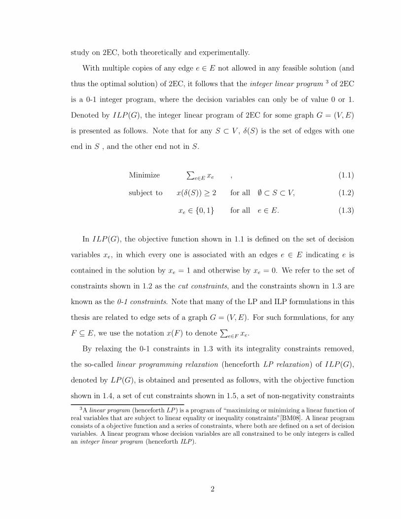
With multiple copies of any edge e ∈ E not allowed in any feasible solution (and

thus the optimal solution) of 2EC, it follows that the integer linear program 3 of 2EC

is a 0-1 integer program, where the decision variables can only be of value 0 or 1.

Denoted by ILP (G), the integer linear program of 2EC for some graph G = (V,E)

is presented as follows. Note that for any S ⊂ V , δ(S) is the set of edges with one

end in S , and the other end not in S.

Minimize∑

e∈E xe , (1.1)

subject to x(δ(S)) ≥ 2 for all ∅ ⊂ S ⊂ V, (1.2)

xe ∈ {0, 1} for all e ∈ E. (1.3)

In ILP (G), the objective function shown in 1.1 is defined on the set of decision

variables xe, in which every one is associated with an edges e ∈ E indicating e is

contained in the solution by xe = 1 and otherwise by xe = 0. We refer to the set of

constraints shown in 1.2 as the cut constraints, and the constraints shown in 1.3 are

known as the 0-1 constraints. Note that many of the LP and ILP formulations in this

thesis are related to edge sets of a graph G = (V,E). For such formulations, for any

F ⊆ E, we use the notation x(F ) to denote∑

e∈F xe.

By relaxing the 0-1 constraints in 1.3 with its integrality constraints removed,

the so-called linear programming relaxation (henceforth LP relaxation) of ILP (G),

denoted by LP (G), is obtained and presented as follows, with the objective function

shown in 1.4, a set of cut constraints shown in 1.5, a set of non-negativity constraints

3A linear program (henceforth LP) is a program of “maximizing or minimizing a linear function ofreal variables that are subject to linear equality or inequality constraints”[BM08]. A linear programconsists of a objective function and a series of constraints, where both are defined on a set of decisionvariables. A linear program whose decision variables are all constrained to be only integers is calledan integer linear program (henceforth ILP).

2

shown in 1.6 and a set of upper bound constraints shown in 1.7.

Minimize∑

e∈E xe , (1.4)

subject to x(δ(S)) ≥ 2 for all ∅ ⊂ S ⊂ V, (1.5)

xe ≥ 0 for all e ∈ E, (1.6)

xe ≤ 1 for all e ∈ E. (1.7)

We use the notation OPT (G) and OPTLP (G) to denote the optimal objective value

4 for ILP (G) and LP (G) respectively.

It is known that 2EC is NP-hard5 [JRV03] and also MAX SNP-hard6 (even for

cubic graphs) [CKK02, BIT13], where a cubic graph is a graph in which every vertex

has degree7 3. This does not only imply that 2EC is very unlikely to be solved in

polynomial time, but also suggests that the existence of a polynomial time approx-

imation scheme8 is highly doubtful. For this reason, looking for reasonably good

solutions, which are not too far from optimal and obtainable efficiently enough be-

comes a more promising approach for obtaining solutions for 2EC that are provably

close to optimal. Note that since 2EC on cubic graphs is the simplest among all 2EC

problems which remains NP-hard, we concentrate on solving 2EC for cubic graphs

in order to learn more about 2EC. For some constant ρ ≥ 1, which is called the ap-

proximation ratio, a ρ-approximation algorithm for 2EC produces a feasible solution

whose objective value is no more than ρ times the optimal objective value [BM08]

(i.e. OPT (G)). It follows that a 1-approximation algorithm produces an optimal

solution. Due to the difficulty of finding OPT (G), it seems impossible to prove that

4Any set of values assigned to the decision variables that satisfies all constraints is referred to asa feasible solution. A feasible solution at which the objective function achieves its optimum is anoptimal solution, and the optimum is called the optimal objective value.

5Please refer to Section 2.1.2 for definitions.6Please refer to Section 2.1.2 for definitions.7The degree of a vertex is the number of edges incident with it.8Please refer to Section 2.1.2 for definitions.

3

such an algorithm always yields a solution within ρ times OPT (G). It follows that a

lower bound for OPT (G) is often a necessary element in designing an approximation

algorithm. For any graph G with n vertices, if there exists one, a Hamilton cycle9 of

G is naturally a minimum 2-edge-connected spanning subgraph of G. It leads to an

obvious lower bound for OPT (G), which is the number of vertices in G, denoted by

n. Note that n is the lowest possible bound for OPT (G), since a Hamilton cycle, if

there exists one, is the minimum-possible size 2-edge-connected spanning subgraph

for any graph. The lower bound of n is employed in [BIT13] and [Huh04], as well as

for the approximation algorithm presented in this thesis.

On the other hand, since LP (G) is a relaxation of ILP (G), the optimal objective

value of LP (G), denoted by OPTLP (G), serves as a relatively tighter lower bound

for OPT (G), i.e., OPTLP (G) ≥ n. For a graph G = (V,E), let α(G) denote the

ratio between OPT (G) and OPTLP (G). This leads to the concept of the integrality

gap of the LP relaxation for 2EC, denoted by α2EC, which is the worst-case ratio

between OPT (G) and OPTLP (G). That is to say, α2EC = max OPT (G)OPTLP (G)

over all G.

As a critical topic throughout this thesis, we studied the integrality gap of the LP

relaxation for 2EC intensively. There are two main reasons this is useful. First, the

integrality gap itself serves as an indicator of the quality of the lower bound given

by LP (G). This is important for methods, such as branch and bound, that depend

on good lower bounds for their success. Secondly, an algorithmic proof for α2EC = k

yields a k-approximation algorithm for 2EC [ABEM06]. In this thesis, we give an

upper bound on the value of α2EC on bridgeless cubic graphs with an algorithmic

proof, while the lower bounds on the integrality gap of 2EC are investigated through

computational studies.

9A Hamilton cycle in a graph G is a cycle that covers all vertices in G. Please refer to Section 2.1.1for its formal definitions.

4

1.1 Contributions

The major contributions of this thesis are as follows:

1. We develop a new 54-approximation algorithm for 2EC on bridgeless cubic

graphs, which constructs a feasible solution of 2EC on a given bridgeless cubic

graph G = (V,E) that contains at most 54|V |−1 edges with two specified edges

included in O(n3) time. It improves upon the previous best approximation ratio

of 54

+ ǫ given by Csaba, Karpinski and Krysta [CKK02] for 2EC on maximum

degree 3 graphs10. Along with the introduction of this algorithm, a theorem in-

dicating that the integrality gap of 2EC is at most 54

for bridgeless cubic graphs

is proved, which defines a tighter upper bound than the integrality gap of the

LP relaxation for 2EC on maximum degree 3 graphs as 54+ ǫ for any fixed ǫ > 0

[CKK02].

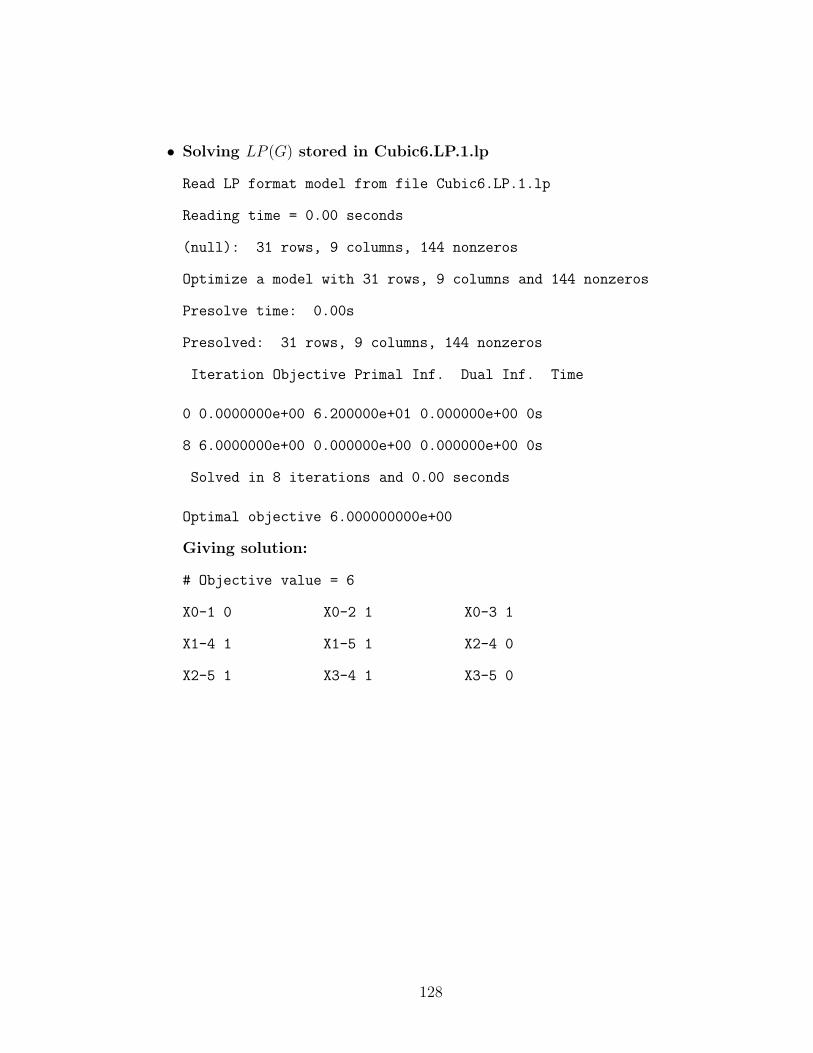
2. Focusing on the integrality gap of the LP relaxation for 2EC, we conduct

a computational study by designing a program that calculates OPT (G) and

OPTLP (G) and thus gives α(G) exactly for all G ∈ G, where G contains all test

cases in three categories:

• General bridgeless graphs for 3 ≤ n ≤ 10;

• Cubic bridgeless graphs for 6 ≤ n ≤ 16; and

• Subcubic bridgeless graphs for 3 ≤ n ≤ 16.

In our experiments, one subcubic graph, G16, stands out. It has 16 vertices and

gives α(G16) = 98, which is the same value as the previous known best lower

bound on the integrality gap of the LP relaxation for 2EC [SV12], with G16

different from the example used in [SV12].

10A maximum degree 3 graph has degree at most 3 everywhere. If the given graph is bridgeless,a maximum degree 3 graph is equivalent to a subcubic graph, in which the degree for any vertex iseither 2 or 3.

5

3. With the knowledge gained from the bottlenecks we faced during the design of

the approximation algorithm mentioned in 1, we provide a family of subcubic

graphs G for which OPT (G)n

= 43

asymptotically, as well as a family of cubic

graphs G for which OPT (G)n

= 76

asymptotically. These two families of graphs

thus suggest that for any approximation algorithm with a performance guaran-

tee of k · n, k = 43

would be the best possible for subcubic bridgeless graphs,

and k = 76

would be the best possible for cubic bridgeless graphs.

4. Using the knowledge gained through the data analysis for the computational

study, we provide two different families of subcubic graphsG for which OPT (G)OPTLP (G)

=

87

asymptotically, which further tightens the lower bound of the integrality gap

to 87. It significantly improves the previous known best lower bound of α2EC for

subcubic graphs from 98

[SV12].

1.2 Outlines

With a literature review on 2EC given in the remainder of this chapter, an overview

of the structure of this thesis is as follows:

In Chapter 2, general definitions and notations that are utilized throughout this

thesis are given in Section 2.1. In Section 2.2, followed by a discussion on their rela-

tionship with 2EC, several problems which are highly related to 2EC are introduced.

In Chapter 3, we first conduct a detailed review in Section 3.1 on a 65-approximation

algorithm for 2EC on 3-edge-connected cubic graphs, which is referred to as Apx2EC

and designed by Boyd, Iwata and Takazawa [BIT13]. As the cornerstone of our

algorithmic studies, a deep analysis on the bottlenecks for generalizing the above

algorithm is demonstrated in Section 3.2. This is followed by our design of a 54-

approximation algorithm for 2EC on bridgeless cubic graphs, which is an extension of

Algorithm Apx2EC, by overcoming the bottlenecks discussed in the previous section.

6

Following this algorithm, a theorem indicating that the integrality gap of 2EC is at

most 54

for bridgeless cubic graphs is proved.

In Chapter 4, with the desire to learn more about the integrality gap of 2EC,

we investigate the worst-case ratio between ILP (G) and LP (G) computationally for

graphs with a small number of vertices. By designing and realizing a program as

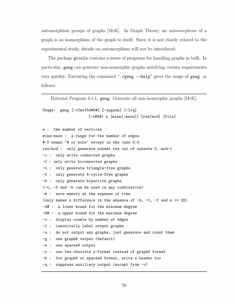
presented in Section 4.1, that generates requested experimental objects with the help

from nauty[McK], and gives optimal solutions to ILP (G) and LP (G) with the aid of

GurobiTMOptimizer [Gur12b], we thus obtained α(G), as the ratio between OPT (G)

and OPTLP (G), for every experimental object G. Following an explicit analysis on

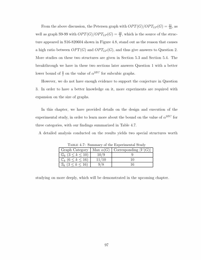
all data given by our program, several discoveries are discussed in Section 4.2.

Finally, by combining the knowledge we gained through both the algorithmic and

computational studies from Chapters 3 and 4, a further study is conducted concerning

the lower bounds on the integrality gap of 2EC by demonstrating four families of

graphs. The latter two families of graphs yields a significant improvement on the

known best lower bound for α2EC on subcubic graphs.

1.3 Literature Review on 2EC

Constant factor approximation algorithms11 for 2EC have been intensively studied.

For an unweighted bridgeless graph G = (V,E) on n vertices, a 2-edge-connected

spanning subgraph of G can be found based on a spanning subtree T of G resulted

from a depth-first-search (henceforth DFS ), which is a widely-used graph traversing

algorithm that starts from an arbitrary vertex as the root and explores as deep as

possible along each branch in prior to backtracking. All non-tree edges are referred to

as back edges, i.e., edges whose one end is an ancestor of the other end in T . By taking

all edges in T and the deepest backward edge from every non-root vertex, a 2-edge-

11A constant factor approximation algorithm is an approximation algorithm whose approximationratio is of a fixed value.

7

connected spanning subgraph of G is obtained with at most 2n−2 edges [VV00]. This

simply gives a 2-approximation algorithm for 2EC with n serving as the lower bound.

Another easy 2-approximation algorithm can be found in [CSS98]. In 1994, Khuller

and Vishkin [KV94] first improved this approximation ratio of 2 to 32

with a better

lower bound obtained from the idea of “tree carving”, by presenting an algorithm also

based on depth-first search but with a stricter scheme for picking back edges. Around

the same time, Garg, Santosh and Singla [GSS93] claimed that with a better lower

bound, which is obtained from an extended idea of “tree carving”, a 54-approximation

algorithm can be achieved, but no complete proof or details were ever provided. In

1998, Cheriyan, Sebo and Szigeti [CSS98] improved the approximation ratio from 32

to

1712

by using an “ear decomposition” [CSS98, SV12] to obtain a feasible solution. The

ratio was later improved to 43

in 2000 by Vempala and Vetta [VV00]. One year later,

Krysta and Kumar [KK01] improved the approximation ratio to 43− ǫ where ǫ = 1

1344

by extending the technique of Vempala and Vetta. In 2003, Jothi, Raghavachari

and Varadarajan claimed to have a 54-approximation algorithm, but their proof was

incomplete, and a complete proof was never provided. Very recently, Sebo and Vygen

[SV12] designed a simpler and more elegant 43-approximation algorithm for 2EC,

along with other results for related problems, by introducing the technique called

“nicer ears” based on the idea of ear decomposition.

In the meantime, research on 2EC has also been conducted for special classes

of graphs, especially on cubic bridgeless graphs, on which 2EC still remains NP-

hard. In 2001, along with their (43− ǫ)-approximation algorithm for 2EC on general

graphs, Krysta and Kumar [KK01] also presented an approximation algorithm for

2EC on cubic graphs with the approximation ratio of 2116

+ ǫ. One year later, Csaba,

Karpinski and Krysta [CKK02] designed a (54

+ ǫ)-approximation algorithm for 2EC

on maximum degree 3 graphs, which are also subcubic graphs considering the input

graph is bridgeless. In 2004, Huh [Huh04] presented an algorithm yielding a solution

8

H to the 2EC on the r-edge-connected (r ≥ 2) graphs G = (V,E) with at most

|V | + |E|−|V |r−1

edges in H . It follows that for r-regular12, r-edge-connected graphs,

the approximation ratio is 54, 4

3, 11

8, 7

5for r = 3, 4, 5, 6 respectively. A more recent

significant improvement came from Boyd, Iwata and Takazawa [BIT13] with a 65-

approximation algorithm for 2EC on cubic 3-edge-connected graphs.

Concerning the integrality gap of 2EC, α2EC, on unweighted graphs, Csaba,

Karpinski and Krysta [CKK02] proved that for maximum degree 3 graphs, the inte-

grality gap of the LP relaxation for 2EC is at most 54

+ ǫ for any fixed ǫ > 0. It was

also stated in [CKK02] that the known best lower bound on 2EC is 109

for maximum

degree 3 graphs (and thus subcubic graphs). In 2012, by giving a 65-approximation

algorithm, Boyd, Iwata and Takazawa defined an upper bound as 65

on the value of

α2EC for 3-edge-connected cubic graphs. Around the same time, Sebo and Vygen

[SV12] proved that α2EC ≤ 43

by providing a 43-approximation algorithm for 2EC on

all bridgeless graphs; and α2EC ≤ 98

by using the same example as shown in Fig-

ure 1 in [ABEM06] with unit weights, which improved the known best lower bound

on α2EC defined by [CKK02]. Most other studies concerning the integrality gap of

the LP relaxation for 2EC are based on 2EC with general cost functions, which are

introduced in detail in Sections 2.2.2 and 2.2.4.

12A r-regular graph is a graph where every vertex is incident to r edges, i.e., every vertex has thesame degree of r.

9

Chapter 2

Preliminaries

This chapter provides definitions and notations that are utilized throughout this the-

sis. This is followed by an introduction to three problems, i.e., minimum size 2-edge-

connected spanning multi-subgraph problem, minimum cost 2-edge-connected spanning

(multi-)subgraph problem and graph traveling salesman problem, that are highly re-

lated to 2EC. Literature reviews on these three problems are also included to discuss

some important studies which motivated and inspired our work.

2.1 General Definitions and Notations

2.1.1 Graphs, Subgraphs and Trees

As defined by Bondy and Murty in Graph Theory [BM08, p. 2]:

A graph G is an ordered pair (V (G), E(G)) consisting of a set V (G) of

vertices and a set E(G), disjoint from V (G), of edges, together with an

incidence function ψG that associates with each edge of G an unordered

pair of (not necessarily distinct) vertices of G. If e is an edge and u and v

are vertices such that ψG(e) = {u, v}, then e is said to join u and v, and

vertices u and v are called the ends of e.

10

In this thesis, we denote a graph by G = (V,E), where V represents the vertex set,

E is the edge set, and the incidence function is implied. Unless stated otherwise, n is

used to denote the number of vertices in G, i.e. n = |V |. Usually a lowercase letter,

such as u or v, is employed to denoted a vertex in a graph. For an edge in a graph

with two ends as u and v, an unordered pair (u, v) is used to denote the edge, or

sometimes it is simply denoted by uv. The following list presents some commonly

used definitions and notations in graph theory, which are utilized in this thesis.

1. An edge is said to be incident with its ends. Two vertices which are incident

with an identical edge are said to be adjacent to each other. Also, two edges

which share an identical end are said to be adjacent to each other.

2. For a pair of adjacent vertices u and v, u is said to be a neighbour of v and vice

versa.

3. For a vertex v ∈ V , δ(v) is used to denote the set of edges incident to v. For

any vertex v ∈ V , the number of edges in δ(v) is referred to as the degree of v,

denoted by dv.

4. For any subset of vertices V ′ ⊆ V , V ′ is used to denote V \ V ′; and δ(V ′) is

used to denote the set of edges with exactly one end in V ′.

5. An edge with identical ends is called a loop; two or more edges ending at the

same pair of vertices are referred to as parallel edges. Unless stated otherwise,

a graph in this thesis contains no loops.

Consider the graph G = (V,E) as shown in Figure 2.1 as an example. This graph

consists of 5 vertices (i.e. n = 5) and 10 edges, where the vertex set V = {0, 1, 2, 3, 4},

the edge set E = {a, b, c, d, e, f, g, h, i, j}, and the incidence function is defined as:

ψG(a) = {1, 2}, ψG(b) = {2, 3}, ψG(c) = {3, 4}, ψG(d) = {4, 0}, ψG(e) = {0, 1},

ψG(f) = {2, 0}, ψG(g) = {1, 3}, ψG(h) = {2, 4}, ψG(i) = {3, 0}, ψG(j) = {1, 4}.

11

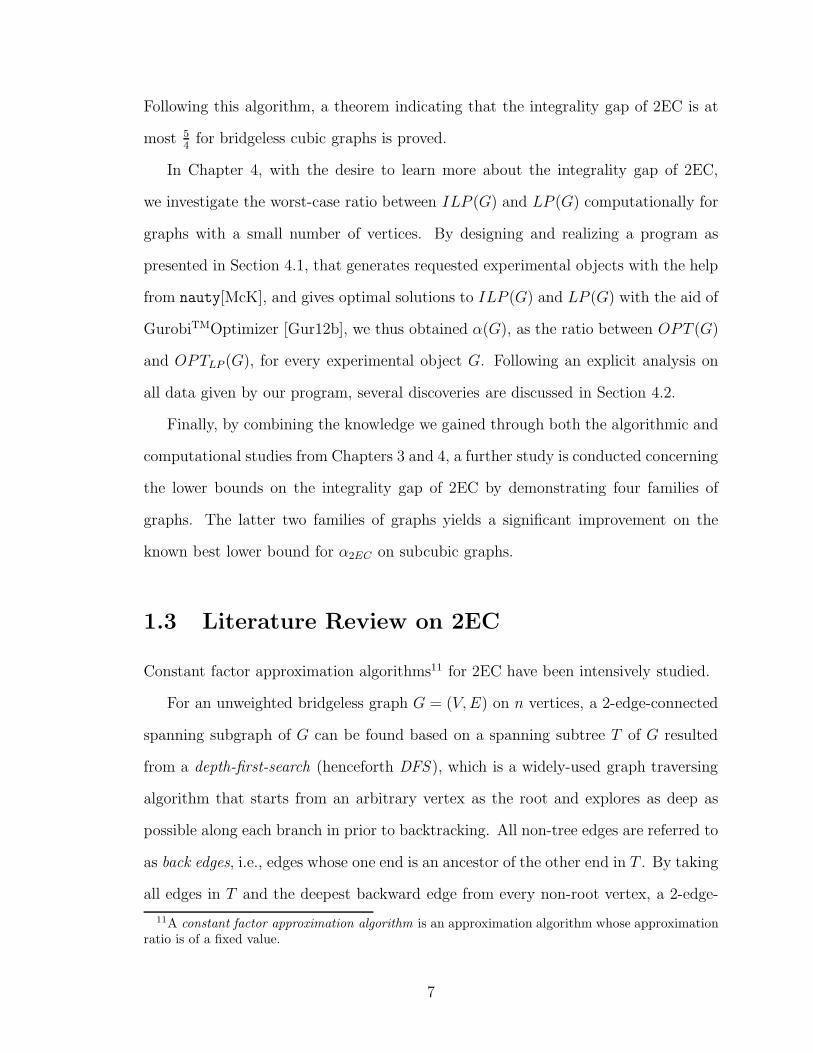
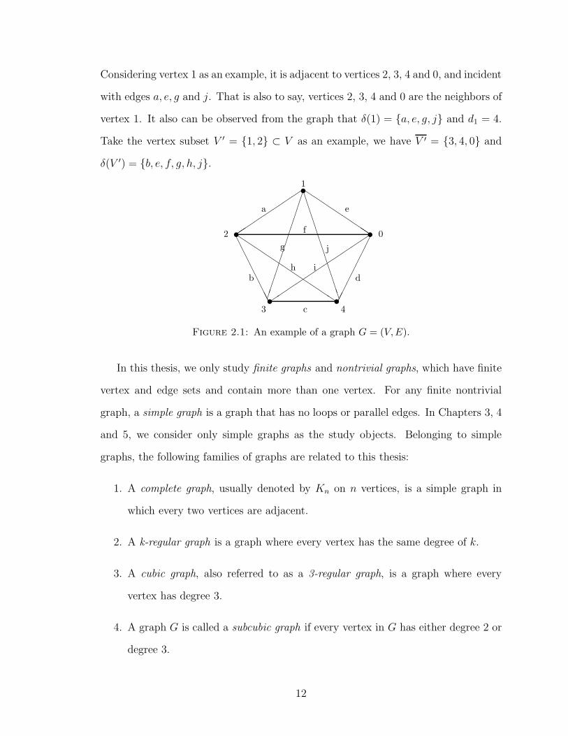
Considering vertex 1 as an example, it is adjacent to vertices 2, 3, 4 and 0, and incident

with edges a, e, g and j. That is also to say, vertices 2, 3, 4 and 0 are the neighbors of

vertex 1. It also can be observed from the graph that δ(1) = {a, e, g, j} and d1 = 4.

Take the vertex subset V ′ = {1, 2} ⊂ V as an example, we have V ′ = {3, 4, 0} and

δ(V ′) = {b, e, f, g, h, j}.

t t

t t

t

✑✑

✑✑

✑✑

✑✑❆❆❆❆❆❆❆❆

✁✁

✁✁

✁✁

✁✁

◗◗

◗◗

◗◗

◗◗✑

✑✑

✑✑

✑✑

✑✑

✑✑

✂✂✂

✂✂✂

✂✂✂

✂✂✂

◗◗

◗◗

◗◗

◗◗

◗◗

❇❇❇❇❇❇❇❇❇❇❇❇

1

02

3 4

a e

db

c

ih

g

f

j

Figure 2.1: An example of a graph G = (V,E).

In this thesis, we only study finite graphs and nontrivial graphs, which have finite

vertex and edge sets and contain more than one vertex. For any finite nontrivial

graph, a simple graph is a graph that has no loops or parallel edges. In Chapters 3, 4

and 5, we consider only simple graphs as the study objects. Belonging to simple

graphs, the following families of graphs are related to this thesis:

1. A complete graph, usually denoted by Kn on n vertices, is a simple graph in

which every two vertices are adjacent.

2. A k-regular graph is a graph where every vertex has the same degree of k.

3. A cubic graph, also referred to as a 3-regular graph, is a graph where every

vertex has degree 3.

4. A graph G is called a subcubic graph if every vertex in G has either degree 2 or

degree 3.

12

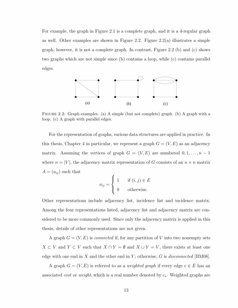
For example, the graph in Figure 2.1 is a complete graph, and it is a 4-regular graph

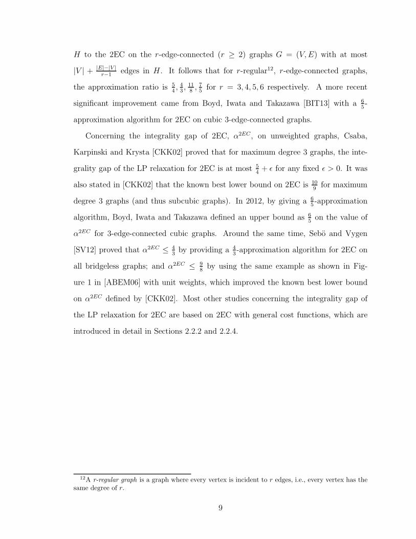
as well. Other examples are shown in Figure 2.2. Figure 2.2(a) illustrates a simple

graph, however, it is not a complete graph. In contrast, Figure 2.2 (b) and (c) shows

two graphs which are not simple since (b) contains a loop, while (c) contains parallel

edges.

(a) (b) (c)

Figure 2.2: Graph examples. (a) A simple (but not complete) graph. (b) A graph with aloop. (c) A graph with parallel edges.

For the representation of graphs, various data structures are applied in practice. In

this thesis, Chapter 4 in particular, we represent a graph G = (V,E) as an adjacency

matrix. Assuming the vertices of graph G = (V,E) are numbered 0, 1, . . . , n − 1

where n = |V |, the adjacency matrix representation of G consists of an n× n matrix

A = (aij) such that

aij =

1 if (i, j) ∈ E

0 otherwise.

Other representations include adjacency list, incidence list and incidence matrix.

Among the four representations listed, adjacency list and adjacency matrix are con-

sidered to be more commonly used. Since only the adjacency matrix is applied in this

thesis, details of other representations are not given.

A graph G = (V,E) is connected if, for any partition of V into two nonempty sets

X ⊂ V and Y ⊂ V such that X ∩ Y = ∅ and X ∪ Y = V , there exists at least one

edge with one end in X and the other end in Y ; otherwise, G is disconnected [BM08].

A graph G = (V,E) is referred to as a weighted graph if every edge e ∈ E has an

associated cost or weight, which is a real number denoted by ce. Weighted graphs are

13

very useful for solving practical problems. The adjacency list can be easily adapted

to represent a weighted graph by storing the weight ce of the edge e = (i, j) ∈ E as

the entry in row i and column j of the adjacency matrix. However, different from the

adjacency matrix for an unweighted graph which has no cost on any edge, for an edge

e /∈ E, it is represented by a nil value in the corresponding matrix entry; although

in practice, it is convenient to use a value such as 0, ∞, or∑

e∈E ce if there exists

ce = 0 for any e ∈ E. In this thesis, unless stated otherwise, our research is based on

unweighted graphs, especially in Chapters 3, 4 and 5. Previous research conducted

on weighted graphs are reviewed in Subsection 2.2.2 for a better understanding of

this problem.

In a graph, a path is “a simple graph whose vertices can be arranged in a linear

sequence in such a way that two vertices are adjacent if they are consecutive in the

sequence and are nonadjacent otherwise”[BM08, p. 4]. A path in a graph G is called

a Hamilton path if it contains all vertices in G. Likewise, a cycle on three or more

vertices is “a simple graph whose vertices can be arranged in a cyclic sequence in

such a way that two vertices are adjacent if they are consecutive in the sequence,

and nonadjacent otherwise”[BM08, p. 4]. Similarly, a Hamilton cycle in a graph

G = (V,E) is a cycle that covers all vertices in G. In this thesis, k-cycle is used to

denote a cycle which contains k vertices.

A graph which does not contain any cycle is referred to as an acyclic graph, which

is also known as a forest. A connected acyclic graph is called a tree. The term node is

used to represent a vertex in a tree. When defining a tree, one of the nodes is usually

selected as the root of the tree, which is denoted by r. Since a tree is acyclic, any

two nodes are connected by exactly one simple path, where no loops or parallel edges

are allowed. For any node v, except the root r, in a tree T , let P (v) denote such a

simple path connecting r and v. If the last edge on P (V ) is (u, v), u is called the

parent of v, and v is called a child of u. Note that because there is exactly one simple

14

path between the root and every other node, every node except the root has exactly

one parent; however, the number of children of a node can be zero or any positive

value. Any node in a tree that has zero children is called a leaf of the tree; and a

non-leaf node is called an internal node. For any node v in T other than the root r,

the length of the simple path P (v) connecting r and v is referred to as the depth of v

in T ; on the other hand, the height of v in T is measured by the number of edges in

the longest simple downward path from v to a leaf. The height of a tree T , denoted

by h, is the height of the root of T [CLRS09].

Following the basic knowledge on graphs presented above, we introduce the con-

cept of subgraphs. A graph H is referred to as a subgraph of the graph G denoted by

H ⊆ G or G ⊇ H , if V (H) ⊆ V (G), E(H) ⊆ E(G), and ψH is the restriction of ψG

to E(H) [BM08, p. 40]. Moreover, a subtree of a graph is a subgraph which is a tree.

Note that any graph is a subgraph of itself.

Generally speaking, there are two operations used to obtain a subgraph of a graph

G, edge deletions and vertex deletions. For any graph G, edge deletion on an edge e ∈

E(G), denoted by G \ e, leads to a subgraph H ⊂ G, where H = (V (G), E(G) \ {e});

while vertex deletion on a vertex v ∈ V (G), denoted by G − v, leads to a subgraph

H ⊂ G, where H = (V (G) \ {v}, E(G) \ δ(v)). In this thesis, G− V ′ where V ′ ⊆ V

is used to denote the deletion of a set of vertices from G, while G \E ′ where E ′ ⊆ E

is used to denote the deletion of a set of edges from G. Figure 2.3 illustrates three

subgraphs of the complete graph G shown in Figure 2.1. Figure 2.3 (a) and (c) are

obtained from edge deletions and Figure 2.3 (b) is obtained from vertex deletions.

A spanning subgraph H of a graph G is a subgraph obtained by edge deletions

only. That is to say, a subgraph H of G is referred to as a spanning subgraph of G

if V (H) = V (G). A spanning tree of a graph G is a subtree of G that contains all

vertices in G. A graph is connected if and only if it has a spanning tree [BM08, p. 106];

while a disconnected graph G has a spanning forest, consisting of a set of spanning

15

b

c

dih

(b) G − {1}

a

c

f

i

(c) G \ {b, d, e, g, h, j}

a

b

c

d

e

f

ih

(a) G \ {g, j}3 4

2 5

1

2

3 4

f5

1

2 5

43

Figure 2.3: Examples of subgraphs of the graph G in Figure 2.1. (a) A subgraph obtainedfrom the edge deletions. (b) A subgraph obtained from the vertex deletion. (c) A treeobtained from the edge deletions.

trees for each connected components1. Consider the graph G shown in Figure 2.1 as

an example, graphs shown in Figures 2.3 (a) and (c) and G itself are all spanning

subgraphs of G, whereas the graph shown in Figure 2.3 (c) is a spanning tree of G

as well. However, the graph shown in Figure 2.3 (b) is a subgraph of G but not its

spanning subgraph.

As two of the very important and fundamental algorithms for graphs, breadth-

first search (BFS henceforth) and depth-first search (DFS henceforth) are two major

strategies for traversals throughout a graph. For any graph G = (V,E), both BFS

and DFS result in a spanning tree of G if G is connected or a spanning forest of G

otherwise.

In graph theory, a spanning graph of a graph G can also be referred to as a factor

of G. A k-factor of a graph is a spanning k-regular subgraph. For a graph G = (V,E),

a 1-factor of the graph G is a spanning subgraph of G consisting of a set of vertex-

disjoint edges; and a 2-factor is a collection of cycles in G that spans all vertices of

G. A 1-factor is also referred to as a perfect matching, where a matching is a set of

vertex-disjoint edges. A matching of a graph G does not necessarily cover all vertices

in G. Note that for cubic graphs, the complement of a 2-factor is a perfect matching.

1For a disconnected graph G, the connected components, or simply the components, of G denotethe vertex set of the maximal connected subgraphs.

16

For a graph G = (V,E), a cut, usually defined by δ(V ′) = {(u, v) : (u, v) ∈ E, u ∈

V ′, v /∈ V ′} for some V ′ ⊂ V [CCPS98], consists of a set of edges E ′ ⊂ E such

that every edge e ∈ E ′ has exactly one end in V ′. The removal of a cut δ(V ′) for

some V ′ ⊂ V in a connected graph G = (V,E) disconnects G into two components,

G[V ′] and G[V ′]. Note that G[V ′] denotes the subgraph of G induced by V ′ ⊂ V ,

i.e., G[V ′] = (V ′, γ(V ′)), where γ(V ′) is the set of edges which have both ends in

V ′. A cut that contains k edges is called a k-edge cut if it does not contain any

other cut as a proper subset. If a cut contains only one edge, this particular edge

is called a cut edge (or a bridge). A graph is called bridgeless if it does not contain

any cut edge. A graph G is said to be k-edge-connected if every cut in G contains

at least k edges. Another way of stating this is that a graph G is k-edge-connected

if and only if G remains connected after the removal of any set of (k − 1) edges.

Trivially, a graph that is k-edge-connected is also (k − 1)-edge-connected. Note that

a graph is 1-edge-connected if and only if it is connected, and a bridgeless graph is

also a 2-edge-connected graph. Consider the graphs shown in Figure 2.3 as examples,

Figure 2.3 (a) is 2-edge-connected, Figure 2.3 (b) is 3-edge-connected, and Figure 2.3

(c) is 1-edge-connected.

Different from a cut of some graph G = (V,E) that consists of a set of edges

E ′ ∈ E, a vertex cut consists of a subset of V that separates some pair of non-

adjacent vertices of G. In another word, a vertex cut of some graph G = (V,E) is

defined by a proper subset R ⊂ V whose removal disconnects G, i.e. G−R contains

more than one component. A vertex cut R which contains k vertices is referred to as

a k-vertex cut ; when k = 1, this particular vertex that forms the 1-vertex cut is called

a cut vertex. Note that a complete graph has no vertex cut. We say a graph G is

k-vertex-connected if every vertex cut in G contains at least k vertices. Consider the

graphs shown in Figure 2.3 as examples, Figure 2.3 (a) is 2-vertex-connected where

{2, 5} forms a 2-vertex cut, Figure 2.3 (b) has no vertex cut, and Figure 2.3 (c) is

17

1-vertex-connected where vertices 2, 3 an 5 are all cut vertices.

2.1.2 NP-Hardness and Approximation Algorithms

For an algorithm, the computational complexity is used to measure the number of

basic computational steps required for the execution of the algorithm [BM08]. For

any algorithm, we usually use O-notation to give an asymptotic upper bound on

its computational complexity, in which the lower order terms and coefficients become

irrelevant [CLRS09]. Given an input of size n, an algorithm is called a polynomial-time

algorithm if the number of steps required to complete the algorithm for a given input

is O(nk) for some non-negative k, which does not depend on n. For example, both

BFS and DFS are polynomial-time algorithms with the computational complexity of

O(|V | + |E|), for an input G = (V,E) with n vertices. Polynomial-time algorithms

are usually considered to be computationally feasible, even for large inputs [BM08].

A problem is said to be solvable in polynomial time if there is a polynomial-time

algorithm for it.

A decision problem is a problem whose answer is either positive or negative. The

class of decision problems that can be solved in polynomial time is usually denoted

by P. On the other hand, the class of NP, where NP denotes “nondeterministic

polynomial”, consist of decision problems “with the property that for any input that

has a positive answer, there is a certificate from which the correctness of this answer

can be derived in polynomial time” [CCPS98, p. 309]. One of the extensively studied

problem in NP is the Hamilton cycle problem (HAM-CYCLE henceforth) [CLRS09],

which questions “Does G have a Hamilton cycle?” for some graph G. Considering

HAM-CYCLE as an example, if the answer to HAM-CYCLE is positive, it can be

verified by giving a Hamilton cycle of G as a certificate, which can be checked in

polynomial time. Therefore it provides a way to check the correctness of the answer

in polynomial time. Note that the class NP includes all problems in the class P, i.e.,

18

P ⊆ NP.

A decision problem Π is called NP-complete if it is in NP and every problem

in NP can be transformed to Π within polynomial time. The procedure of the

transformation is usually referred to as polynomial-time reduction. Irrelevant to this

thesis, the details of the polynomial-time reduction will not be given here. In other

words, a problem Π is NP-complete if Π ∈ NP and an algorithm for solving Π can be

converted into one for solving any other problem in the class of NP. It implies that if

any NP-complete problem can be proved to be solvable in polynomial time, then all

problems in NP can be solved in polynomial time, which leads to P = NP. However,

no polynomial-time algorithm has been found for any NP-complete problem until

now, which leaves the P versus NP problem a major unsolved problem in computer

science. Note that HAM-CYCLE ∈ NP-complete holds as well.

In real life, not all problems are decision problems. As a matter of fact, many

problems of interest are optimization problems, in which “each feasible solution has

an associated value, and we wish to find a feasible solution with the best value”

[CLRS09]. For an optimization problem Π, we use Π ∈ NP-hard to indicate Π is

at least as hard as an NP-complete problem. An optimization problem cannot be

referred to as an NP-complete problem, because this term applies only to decision

problems [KT05]. Note that an NP-hard problem does not necessarily belong to

NP, since it might not be a decision problem. An NP-complete problem belongs to

both NP and NP-hard [BW05].

A famous example for NP-hardness is the symmetric traveling salesman problem.

Given the complete graph Kn = (V,E) on n vertices with non-negative real cost ce

associated with every e ∈ E, the Symmetric Traveling Salesman Problem (STSP)

consists of finding a Hamiltonian cycle in Kn with minimum cost. Symmetric travel-

ing salesman problems on some graph Kn are referred to as metric STSP if the costs

on edges in Kn satisfy the triangle inequality. It is known that the STSP, includ-

19

ing the metric STSP, is NP-hard [BB08]. In Subsection 2.1.4, we will introduce a

mathematical formulation of the problem and give more details.

Since many problems of practical significance are NP-complete or NP-hard,

which are unlikely to be solved efficiently enough, approximation algorithms are com-

monly applied to solve such problems. For any NP-hard problem, a ρ-approximation

algorithm is a polynomial algorithm which delivers a solution whose cost is at most

ρ times the optimum. The factor ρ is usually called the approximation ratio. Since

the cost of the optimal solution is normally unknown, a bound for the optimal solu-

tion is often involved in an approximation algorithm. Let x denotes the value of the

bound utilized in a ρ-approximation algorithm, ρ ·x is referred to as the performance

guarantee of this approximation algorithm.

Based on the property of the approximation ratio, there are three types of ap-

proximation algorithms: full polynomial time approximation scheme, polynomial time

approximation scheme and constant-factor approximation algorithm. Quoted from

[ALM+98], we give the formal definitions for the above three approximation schemes.

A full polynomial time approximation scheme is an algorithm that, for

any given ǫ > 0, approximates the problem within a factor 1 + ǫ in time

that is polynomial in the input size and 1/ǫ.

A polynomial time approximation scheme is an algorithm that, for any

given ǫ > 0, approximates the problem within a factor 1 + ǫ in time that

is polynomial in the input size (and could depend arbitrarily upon 1/ǫ).

A constant-factor approximation algorithm are algorithms which, for some

fixed constant c > 1, are able to approximate the optimal solution to

within a factor c in polynomial time.

[ALM+98]

According to the existence of the different types of approximation algorithms, a prob-

20

lem can be divided in different classes. A problem with only constant-factor approx-

imation algorithms belongs to the class APX, a problem with a polynomial time

approximation scheme falls into the class PTAS, and a problem with a full polyno-

mial time approximation scheme is of the class FPTAS. It follows from the definition

that FPTAS ⊂ PTAS ⊂ APX. Note that PTAS = APX if and only if P = NP

[ALM+98]. In simpler terms, a problem Π ∈ APX only has polynomial-time algo-

rithms with the approximation ratio as some fixed factor; a problem Π ∈ PTAS has

polynomial-time algorithms delivering solutions within every fixed factor greater than

1 of the optimum. A problem is said to be MAX SNP-hard if it has no polynomial

time approximation scheme unless P = NP, which is considered very unlikely so far.

2.1.3 Linear Program and Integer Linear Program

Many problems in real life are in the form of maximizing or minimizing an objective

by searching for an optimum allocation of the limited resources under competing

constraints. Linear program came to the public attention with a variety of such

practical applications. A linear program (henceforth LP) is “a problem of maximizing

or minimizing a linear function of real variables that are subject to linear equality or

inequality constraints”[BM08, p. 197]. Generally, an LP consists of a linear function

which is referred to as the objective function, a set of real decision variables and a

set of constraints presented in the form of linear equalities or linear inequalities. We

call a problem a maximization linear program if we are to maximize the objective

function, and a minimization linear program if we are to minimize the objective

function. Mathematically, any LP with n variables and (m+ n) constraints, either a

maximization linear program or a minimization linear program, can be described in

the following standard form (Expression 2.1) by simple substitutions. We denote an

21

LP in the standard form by a tuple (A,b, c).

maximize cTx

subject to Ax ≤ b

x ≥ 0,

(2.1)

where A = (aij) is an m × n matrix, b = (bi) is a m-vector, and cT = (cj) and

x = (xj) are both n-vectors for i = 1, 2, ..., m and j = 1, 2, ..., n. In the standard form

presented above, the first line, as the inner product of two vectors, is the objective

function, and the second and the third lines are the constraints. More specifically,

the third line contains n non-negativity constraints, which means that each entry of

the vector x must be non-negative in the standard form. Since it is irrelevant to this

thesis, the method of converting an LP to its standard form will not be introduced

here. However, it can be found in [CLRS09, p. 852]. Note that in this thesis, for

the ease of understanding 2EC and its related problems, which are all minimization

problems, it is not necessary to have their LPs or ILPs written in the standard form.

A setting of the variables x to values which satisfy all the constraints is referred

to as a feasible solution, while a setting of the variables x to values which fail to

satisfy some constraint is referred to as an infeasible solution. A solution x leads to

an objective value cTx. A feasible solution, denoted by x∗ is referred to as an optimal

solution if its objective value is maximum (or minimum, for a minimization problem)

over all feasible solutions, and we call its objective value cTx∗ the optimal objective

value.

Associated with every LP, there is another LP, which is referred to as the dual of

the original LP. The original LP is also known as the primal. For example, for the

22

LP in the standard form shown in Expression 2.1, its dual is presented below.

minimize bTy

subject to Ay ≥ c

y ≥ 0,

(2.2)

where A, b and c represents the same thing as they do in the primal LP, and y is

an m-vector. It follows that for a primal LP consisting of n variables and (m + n)

constraints, its dual consists of m variables and (n + m) constraints, among which

m constraints are non-negativity constraints. Consider LP (G) given in 1.4 - 1.7 as

an example, which is the LP relaxation for ILP (G) as introduced in Chapter 1. Its

corresponding dual LP, denoted by LPdual(G), is presented as follows:

maximize 2∑

∅⊂S⊂V yS, (2.3)

subject to∑

e∈δ(S) yS ≥ 1 for all e ∈ E, (2.4)

ys ≥ 0 for all ∅ ⊂ S ⊂ V. (2.5)

LPdual(G) takes all proper non-empty subset ∅ ⊂ S ⊂ V as decision variables, and

consists of the maximization objective function shown in 2.3, a set of constraints

associated with every e ∈ G shown in 2.4, and a set of non-negativity constraints

shown in 2.5.

The concept of duality provides a way to prove that a solution to the primal LP

is indeed optimal. Thanks to von Neumann (1928)[BM08], Theorem 2.1.1 guarantees

that one can always certify optimality of a primal solution by providing a dual solution

which has the same objective value as the objective value of the primal solution.

Theorem 2.1.1 (Duality Theorem [BM08]). If an LP has an optimal solution,

then its dual also has an optimal solution, and the optimal values of these two LPs

are equal.

23

The simplex algorithm (also known as the simplex method), invented by George

Dantzig in 1947, is one of most commonly-used algorithms for solving the LP. In

1972, Klee and Minty [KM72] have provided an example demonstrating that the

worst-case complexity of the simplex algorithm is exponential, which leads to the

fact that the simplex method is not a polynomial algorithm. However, despite the

worst-case performance, the simplex algorithm performs very well in practice. [IC94].

Later in 1979, LP was proved to be possible to solve in polynomial time in the worst

case by L.G. Khachian [Kha79] using the ellipsoid algorithm. To run the ellipsoid

algorithm on the LP relaxation of 2EC, LP (G), on some graph G = (V,E), we need

to be able to decide, given x ∈ RE , whether x satisfies all constraints of LP (G). This

decision problem is also known as the separation problem. It is known [BP90] that,

since the separation problem for the cut constraints can be solved in polynomial time

using the procedure given by Gomory and Hu [GH61], LP (G) can be optimized in

polynomial time by using the ellipsoid algorithm2. However, it is very slow in practice.

Even though the ellipsoid algorithm is of significant theoretical importance, it does

not appear to be competitive with the simplex algorithm in practice [CLRS09]. It

also follows that there does not exist a polynomial-time algorithm for solving LP (G)

very efficiently.

A larger breakthrough was brought by N. Karmarkar [Kar84] in 1984 with the

introduction of his revolutionary interior-point method. Even though Karmarkar’s

interior-point method was proved to be a polynomial-time algorithm and seemed

to perform faster than ellipsoid algorithm, it still cannot beat the simplex method

practically.

Similar to the LP, an integer linear program (henceforth ILP) has the same form

as an LP but with the added restriction that the decision variables must be integer-

valued. An ILP is called 0-1 integer program or binary integer program (henceforth

2For a description of the general approach, please refer to [GLS81].

24

BIP), if all its variables are restricted to be either 0 or 1. Presented below is an ILP

and a BIP in their standard forms respectively.

maximize cTx

subject to Ax ≤ b

x ≥ 0

x integer,

(2.6)

maximize cTx

subject to Ax ≤ b

x ≥ 0

x ∈ {0, 1}.

(2.7)

However, different from the LP, it is known that solving an ILP is NP-hard in

general.[BW05] As a special case, the 0-1 integer program is one of Karp’s 21 NP-

complete problems [Kar72].

2.1.4 Integrality Gap

For an ILP, by dropping its integrality constraints we can obtain a related linear

program for the ILP, which is called linear programming relaxation (henceforth LP

relaxation). In particular, for a 0-1 integer program, one can obtain its LP relaxation

by removing the constraints of x ∈ {0, 1} and replacing them with the constraints of

x ≥ 0 and x ≤ 1. The maximum ratio between the optimal objective value of the

integer program and that of its LP relaxation is called the integrality gap of the LP

relaxation.

The concept of LP relaxation is of significant importance for the reason that it

transforms an NP-complete problem into a related problem that is often solvable in

25

polynomial time. The solution to the relaxed LP often gives an upper (or a lower)

bound for the original maximization (or minimization) integer linear program.

2.2 Related Problems

Considering their particularly close connections to 2EC, the following three 2EC-

related problems are introduced in this section: the minimum size 2-edge-connected

spanning multi-subgraph problem (M2EC), the minimum cost 2-edge-connected span-

ning (multi-)subgraph problem (C2EC), and the graph traveling salesman problem

(graph TSP). A discussion on the relationship between 2EC along with M2EC, C2EC

and graph TSP is given in Subsection 2.2.4.

2.2.1 The Minimum Size 2-edge-connected Spanning Multi-

Subgraph Problem

Given an unweighted connected graphG = (V,E), the minimum size 2-edge-connected

spanning multi-subgraph problem (henceforth M2EC ) consists of finding a 2-edge-

connected spanning multi-subgraph H of G with minimum number of edges, where

the multi-subgraph refers to a subgraph of G which allows multiple copies of an edge

to be chosen. Formulated below is the ILP for the M2EC, which is denoted by

ILPM2EC(G) for some graph G = (V,E).
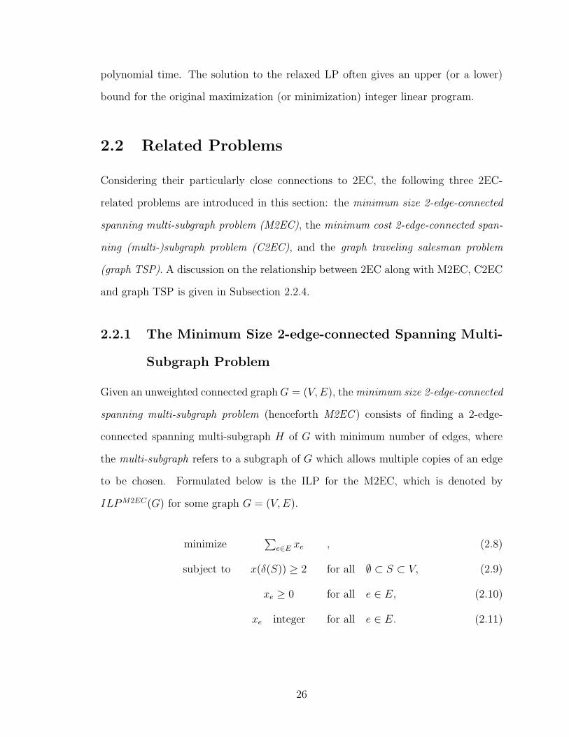
minimize∑

e∈E xe , (2.8)

subject to x(δ(S)) ≥ 2 for all ∅ ⊂ S ⊂ V, (2.9)

xe ≥ 0 for all e ∈ E, (2.10)

xe integer for all e ∈ E. (2.11)

26

Note that xe is the decision variable of ILPM2EC(G) associated with every edge e ∈ E,

which indicates the number of copies of edge e included in the solution. Similar to

ILP (G), the set of constraints shown in 2.9 is referred to as the cut constraints;

differently, the set of constraints shown in 2.10 is known as the non-negativity con-

straints, and the set of constraints shown in 2.11 is called the integrality constraints.

The LP relaxation of M2EC, denoted by LPM2EC(G) for a graph G = (V,E), can be

obtained by dropping the set of constraints shown in 2.11. We use OPTM2EC(G) and

OPTM2ECLP (G) to denote the optimal objective value of ILPM2EC(G) and LPM2EC(G)

respectively. The integrality gap of M2EC, i.e., maximum OPT M2EC(G)

OPT M2EC

LP(G)

over all G, is

denoted by αM2EC.

It is obvious that a spanning subgraph H as the solution to M2EC contains two

copies of each cut edge in G. However, for an edge e ∈ E which is not a cut edge, it

is not necessary to have it presented as parallel edges in the solution. That is to say,

for M2EC, if the graph is bridgeless, there is always an optimal solution that does

not use multiple edges. Lemma 2.2.1 proves that such an optimal solution of M2EC

on a bridgeless graph always exists.

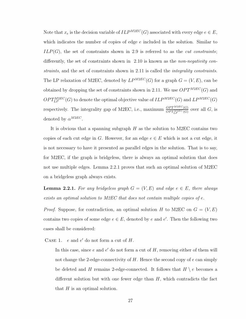
Lemma 2.2.1. For any bridgeless graph G = (V,E) and edge e ∈ E, there always

exists an optimal solution to M2EC that does not contain multiple copies of e.

Proof. Suppose, for contradiction, an optimal solution H to M2EC on G = (V,E)

contains two copies of some edge e ∈ E, denoted by e and e′. Then the following two

cases shall be considered:

Case 1. e and e′ do not form a cut of H .

In this case, since e and e′ do not form a cut of H , removing either of them will

not change the 2-edge-connectivity of H . Hence the second copy of e can simply

be deleted and H remains 2-edge-connected. It follows that H \ e becomes a

different solution but with one fewer edge than H , which contradicts the fact

that H is an optimal solution.

27

Case 2. e and e′ form a cut of H .

Let δ(R) = {e, e′}, R ⊂ V be the cut that e and e′ form, where R contains

exactly one end of e and e′. Since G is bridgeless, there must exist another

edge f ∈ E that is not identical with e and has exactly one end belonging to R

and the other one belonging to R; because otherwise e will be a cut edge whose

removal disconnects R and R. By simply replacing e′ by f , we can avoid the

existence of double copies of e. The newly-generated spanning subgraph remains

2-edge-connected and has the same number of edges as H , which means it is

also an optimal solution.

It follows that in a minimum size 2-edge-connected spanning subgraph of some bridge-

less graph G = (V,E), multiple copies of any edge e ∈ E is always avoidable. Hence

there always exists an optimal solution to M2EC that does not contain parallel edges

for any bridgeless graph.

It follows from Lemma 2.2.1 that for bridgeless graphs, 2EC and M2EC are equiv-

alent, and thus OPT (M2EC) = OPT (2EC).

M2EC is also known to be both NP-hard [SV12] and also MAX SNP-hard (even

for cubic graphs) [CKK02]. The previous research and the obtained results reviewed

in Section 1.3 for 2EC also apply to M2EC.

2.2.2 The Minimum Cost 2-edge-connected Spanning (Multi-

)Subgraph Problem

Given a weighted complete graph Kn = (V,E) on n vertices, let ce ∈ R, ce 6= 0 be a

set of costs associated with every edge e ∈ E. The minimum cost 2-edge-connected

spanning (multi-)subgraph problem (henceforth C2EC ) is that of finding a 2-edge-

connected spanning multi-subgraph of Kn of minimum cost with respect to the costs

on edges [ABEM06]. The problem C2EC on some graph Kn is referred to as metric

28

C2EC if the costs on edges in Kn satisfy the following triangle inequality:

c(x,y) + c(y,z) ≥ c(x,z) for any three vertices x, y, z ∈ V. (2.12)

For a solution to metric C2EC on some complete graph Kn = (V,E), multiple copies

of edges become unnecessary. This is because for every edge e = (u, v) ∈ E, ce is no

greater than the cost of the shortest path between u and v. We formulate C2EC with

an ILP as follows, denoted by ILPC2EC(Kn) for some complete graph Kn = (V,E)

with n vertices.

minimize∑

e∈E cexe , (2.13)

subject to x(δ(S)) ≥ 2 for all ∅ ⊂ S ⊂ V, (2.14)

xe ≥ 0 for all e ∈ E, (2.15)

xe integer for all e ∈ E. (2.16)

In the above formulations, with 2.13 given as the objective function of C2EC, 2.14

represents all cut constraints, 2.15 gives the set of all non-negativity constraints,

and 2.16 gives all integer constraints. By replacing constraints shown in 2.15 and 2.16

with

xe ∈ {1, 0} for all e ∈ E,

the ILP formulation for metric C2EC is obtained, which is a binary integer program.

Similarly to ILP (G), by dropping constraints in 2.16, the corresponding LP re-

laxation of ILPC2EC(Kn), denoted by LPC2EC(Kn), is obtained. For a complete

graph Kn = (V,E) with n vertices, OPTC2EC(Kn) and OPTC2ECLP (Kn) are used to

denote the optimal objective value of ILPC2EC(Kn) and LPC2EC(Kn) respectively.

The integrality gap of the LP relaxation for C2EC, denoted by αC2EC , is defined as

29

follows, which is over all Kn and over all cost functions.

αC2EC = maxc>0

OPT (G)

OPTLP (G)over all G.

C2EC is also known to be NP-complete and MAX SNP-hard [CL99]. In 1982,

Frederickson and Ja Ja [FJ82] first designed a 32-approximation algorithm for the

metric C2EC. Later in 1998, Jain [Jai01] presented a 2-approximation algorithm for

generalized Steiner network problems for finding a minimum-cost spanning subgraph

with “at least a specified number of edges in each cut” [Jai01], which includes the

problem of finding a minimum cost k-edge-connected spanning subgraph, and thus

includes C2EC.

Meanwhile, more research has been conducted considering the integrality gap of

C2EC, i.e. αC2EC . However, except that 65≤ αC2EC ≤ 3

2[ABEM06], not much is

known so far. As integrality gap is defined for minimum 2-edge-connected spanning

subgraph problem over all cost functions, αC2EC also applies for 2EC, which is a

special case of C2EC with cost 1 on every edge in the graph G, and infinity on edges

not in G. As mentioned in [CR98] and [ABEM06], a very useful and interesting

result follows from a result of Cunningham [MMP90] and the Parsimonious Prop-

erty presented by Goemans and Bertsimas [GB90] in 1990, indicating that when the

costs on the edges satisfy the triangle inequality, there exists an optimal solution for

LPC2EC(Kn)3 which is also feasible and hence optimal for SEP (Kn)4 [ABEM06]. In

addition, they also conjectured with supportive explanation that the αC2EC , as the

integrality gap of the C2EC, is 43. It was also mentioned that a family of cost functions

that asymptotically shows αC2EC ≥ 65

can be demonstrated in [CR98]. Later in 2002,

Alexander, Boyd and Elliott-Magwood [ABEM06] confirmed αC2EC ≥ 65

asymptot-

ically by illustrating a different family of cost functions. Exact value for the ratios

3refers to the LP relaxation defined by 2.13 - 2.15.4refers to the LP relaxation for the traveling salesman problem defined by 2.18 - 2.21 in

Subsection 2.2.3.

30

between OPTC2EC(Kn) and OPTC2ECLP (Kn) for small values of n up to 10 and a tight

lower bound for αC2EC are also presented in [ABEM06].

2.2.3 The Graph Traveling Salesman Problem

Given a complete graph Kn = (V,E) with a cost ce associated with every edge e ∈ E,

the traveling salesman problem (henceforth TSP) consists of finding a Hamilton cycle

of Kn of minimum cost. A systematic and precise introduction and literature reviews

on this problem and its variations can be found in [LLKS85]. Note that in this thesis

only symmetric traveling salesman is considered, where no order for the two ends of

any edge in the underlying graph is defined.

As one of the most famous and fundamental problems in combinatorial optimiza-

tion, TSP has been intensively studied for decades, especially for a special case called

the metric traveling salesman problem (henceforth metric TSP), in which the triangle

inequality 2.12 is added as an additional condition on the input graphs. That is to

say, given a weighted complete graph Kn = (V,E) with costs associated with all edges

which satisfy inequality 2.12, metric TSP is to find a minimum-cost Hamilton cycle

of Kn [BM08].

As a relaxation of metric TSP, the graph traveling salesman problem is consider-

ably related to 2EC. Given an unweighted connected graph G = (V,E), defining the

cost between two vertices as the number of edges on the shortest path between them

yields a complete weighted graph on V , which is called the the metric completion of G

[BSSS12]. The graph traveling salesman problem (henceforth graph TSP), is to find

a Hamilton cycle of minimum cost in the metric completion of a given unweighted

connected graph G. It is equivalent to formulate this problem as finding a spanning

Eulerian5 multi-subgraph H = (V,E ′) in a given unweighted graph G = (V,E) with

the minimum number of edges.

5An Eulerian graph is a connected graph G = (V, E) in which the degree of every vertex v ∈ V

is even.

31

As Metric TSP is known to be NP-hard and MAX SNP-hard [LLKS85], even

for graph TSP [PY93], a huge amount of research has been done, striving for better

approximation algorithms for this problem 6. Although no improvements have been

discovered for more than three decades on the 32-approximation algorithm described

by Christofides [Chr76] for the metric, some progress for graph TSP has been given

very recently. In 2005, focusing on graph TSP on 3-edge-connected cubic graphs,

Gamarnik, Lewenstein and Maxim [GLS05] first improved the approximation ratio

from 32

to (32− 5

389) (approximately 1.487). It was followed by Boyd, Sitters, van der

Ster and Stougie [BSSS12] with their 43-approximation algorithm for all cubic graphs

by using polyhedral techniques. Other previous studies conducted for graph TSP

on special classes of graphs can also be found in [BSSS12]. Around the same time,

Momke and Svensson [MS11] improved the approximation ratio for graph-TSP on

general graphs to 1.461 based on a polyhedral idea, along with a 4/3-approximation

algorithm for this problem on subcubic graphs as a side result. In 2012, based on an

improved analysis of the approach presented in [MS11], Mucha [Muc12] gave a better

lower bound on the approximation ratio to 139

(approximately 1.444) for graph TSP

on general graphs. This ratio was later improved by Sebo and Vygen [SV12] with a

75-approximation algorithm.

2.2.4 Relationship between M2EC, C2EC, Graph TSP and

2EC

The relationship between 2EC, M2EC and C2EC is pretty straight-forward. Among

all these three problems, C2EC is considered as the generalized form of the former

two. The problem M2EC can be considered as a special case of C2EC in a way that

an input graph G = (V,E) for M2EC holds the cost 1 for all edges shown in G, while

6In general, the TSP cannot be approximated in polynomial time to within any constant unlessP = NP [BSSS12]

32

the cost ∞ for all edges not shown in G. As an even more relaxed version, 2EC

requires that an input graph does not only hold such cost functions, but also features

2-edge-connectivity (i.e. an input graph is required to be bridgeless). It leads to

2EC ⊆M2EC ⊆ C2EC, (2.17)

which indicates that any algorithms for either C2EC or M2EC applies for 2EC. This

relationship also has significant meaning on the investigation of the integrality gap

of the LP relaxation for 2EC, to which the integrality gap of the LP relaxation for

C2EC applies.

On the other hand, with 2EC being a relaxation of the graph TSP, any optimal

solution of graph TSP in a bridgeless graph G leads to a feasible solution to 2EC on

G with at most the same number of edges [SV12]. Consider the LP relaxation for

C2EC given in 2.13 - 2.15. By changing those cut constraints in 1.5 to equality for

all S ⊂ V where S contains exactly one vertex, we obtain the following LP relaxation

for TSP, which is also known as the subtour relaxation [CR98] or subtour elimination

problem.

minimize∑

e∈E cexe , (2.18)

subject to x(δ(v)) = 2 for all v ∈ V, (2.19)

x(δ(S)) ≥ 2 for all ∅ ⊂ S ⊂ V, (2.20)

xe ≥ 0 for all e ∈ E. (2.21)

It leads to the other important connection between graph TSP and 2EC that lies on

the well-known 43

TSP conjecture presented as follows:

Conjecture 2.2.2. The integrality gap of the subtour relaxation for metric TSP is

at most 43.

33

Following from Conjecture 2.2.2, in 1998, Carr and Ravi [CR98] gives a related

conjecture based on Conjecture 2.2.2 as follows:

Conjecture 2.2.3. [CR98] The minimum cost of a 2-edge connected subgraph is

within 43

times the cost of the optimal subtour solution for the TSP.

Conjecture 2.2.3 suggests that the integrality gap of the LP relaxation for metric

C2EC is at most 43. With Conjecture 2.2.2 implying Conjecture 2.2.3, both remain

unsolved. However, it is suggested [CSS98] that if Conjecture 2.2.3 holds, the inte-

grality gap of the LP relaxation for 2EC is at most 43. Therefore, the 4

3-approximation

algorithm given by Vampala and Vetta [VV00], and the 43-approximation algorithm

given by Sebo and Vygen [SV12], are of significant importance for lending support to

Conjecture 2.2.3, and thus to the 43

TSP conjecture.

In this chapter, with basic knowledge given for graphs, computational complexity,

linear program and integer linear program, and integrality gap for this thesis, we

presented the formal definition for the 2-edge-connected spanning subgraph problem

on both unweighted and weighted graphs. The following cognition can be summarized

with the knowledge gained through Chapters 1 and 2.

1. For 2EC, as well as M2EC, the best known approximation ratio with detailed

proof is 43

[VV00, SV12] for general graphs, 65

for 3-edge-connected cubic graphs

[BIT13], and 54+ ǫ for any fixed ǫ > 0 for maximum degree 3 graphs. The other

interesting finding worth our attention is that Csaba et al. stated that the worst

known lower bound on the integrality gap for 2EC is 109

on subcubic graphs,

which is later improved to 98

by Sebo and Vygen [SV12]. Thus the special family

of graphs, which is derived from our computational study and gives the ratio of

87

between OPT (G) and OPTLP (G), is of some significance.

2. For C2EC, the best known approximation algorithms gives approximation ratio

34

of 2 [KV94, Jai01] for general and 32

for the metric case [FJ82]. It is also known

that the integrality gap for C2EC falls in the range between 65

and 32.

3. For graph TSP, the best-known approximation algorithm has the approximation

ratio of 75, due to Sebo and Vygen [SV12].

35

Chapter 3

A 5/4-Approximation Algorithm

for 2EC on Bridgeless Cubic

Graphs

In this chapter, our algorithm is based on the 65

Algorithm Apx2EC for 2EC on

3-edge-connected cubic graphs [BIT13] due to Boyd, Iwata and Takazawa. In Sec-

tion 3.1, we give an overview of the algorithm Apx2EC. In Section 3.2, we discuss

the reasons that Apx2EC cannot be used to obtain a 65-approximation algorithm for

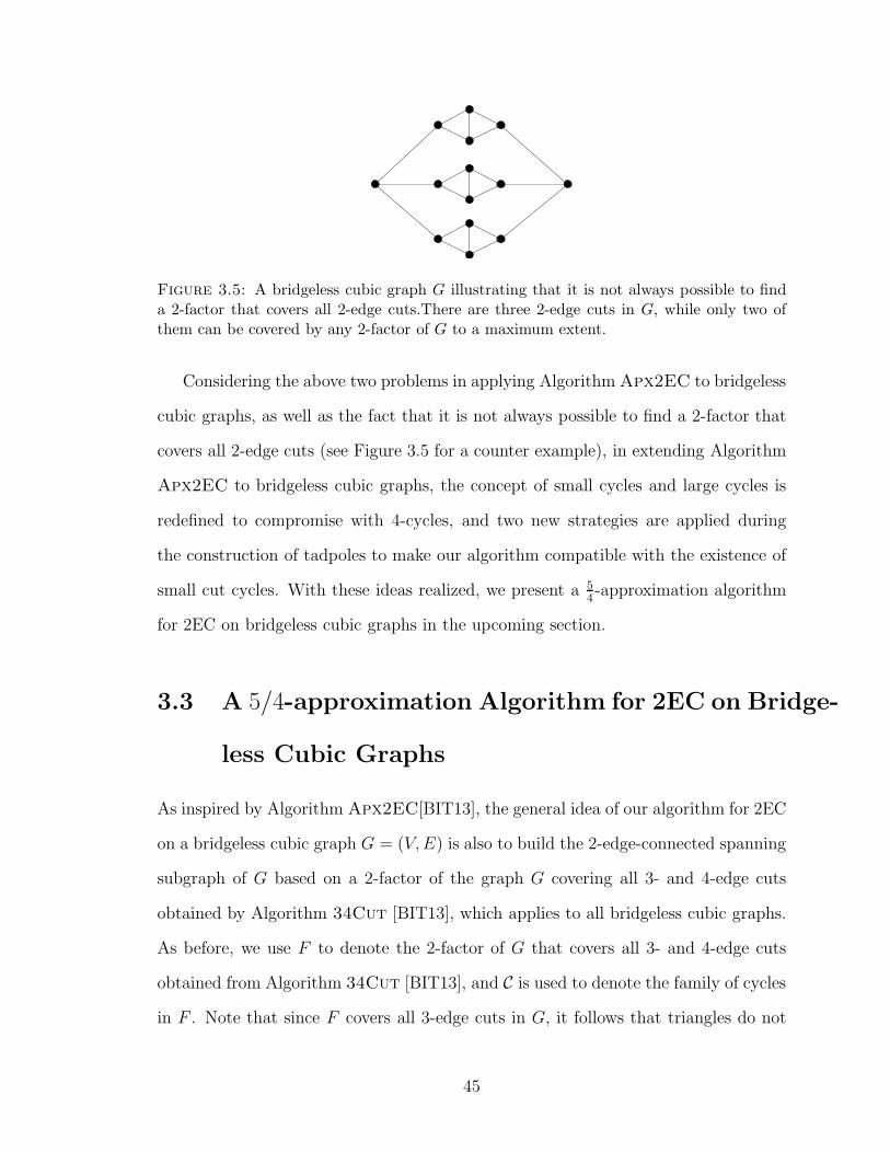
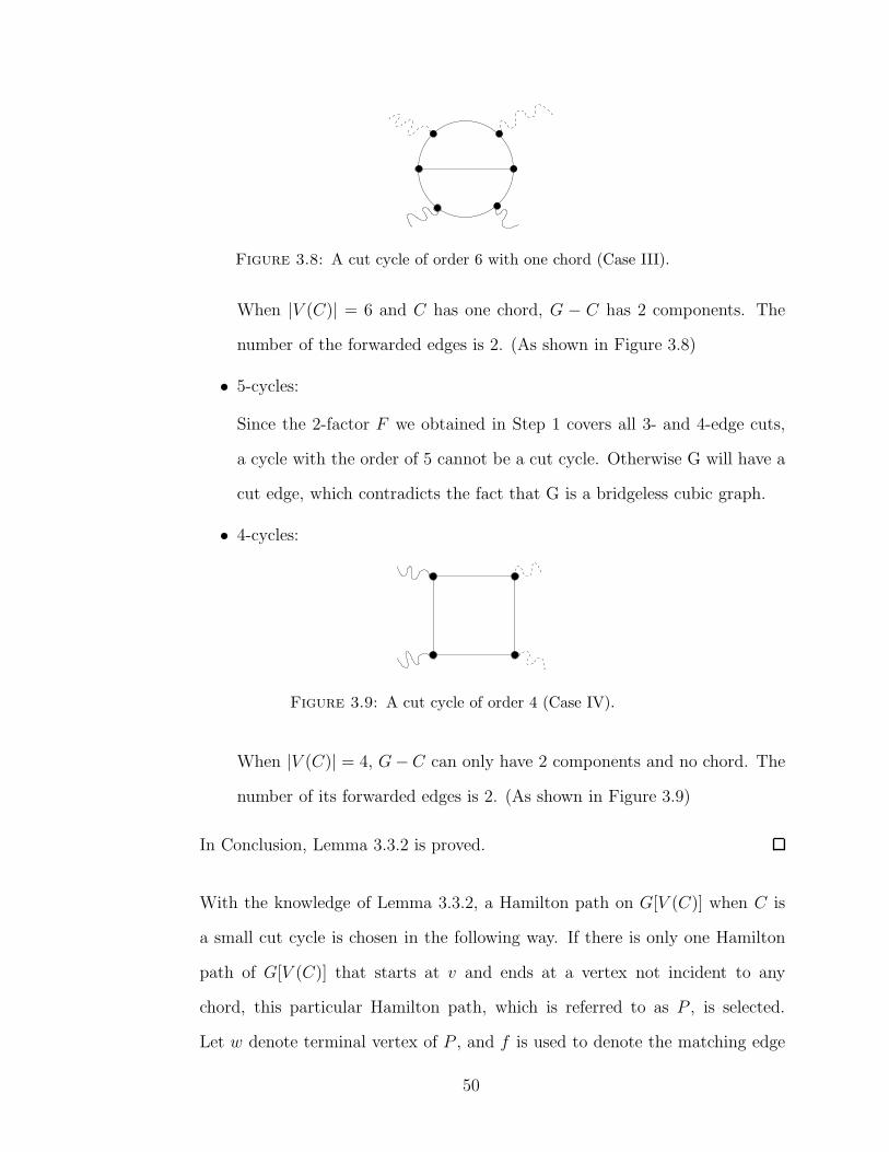
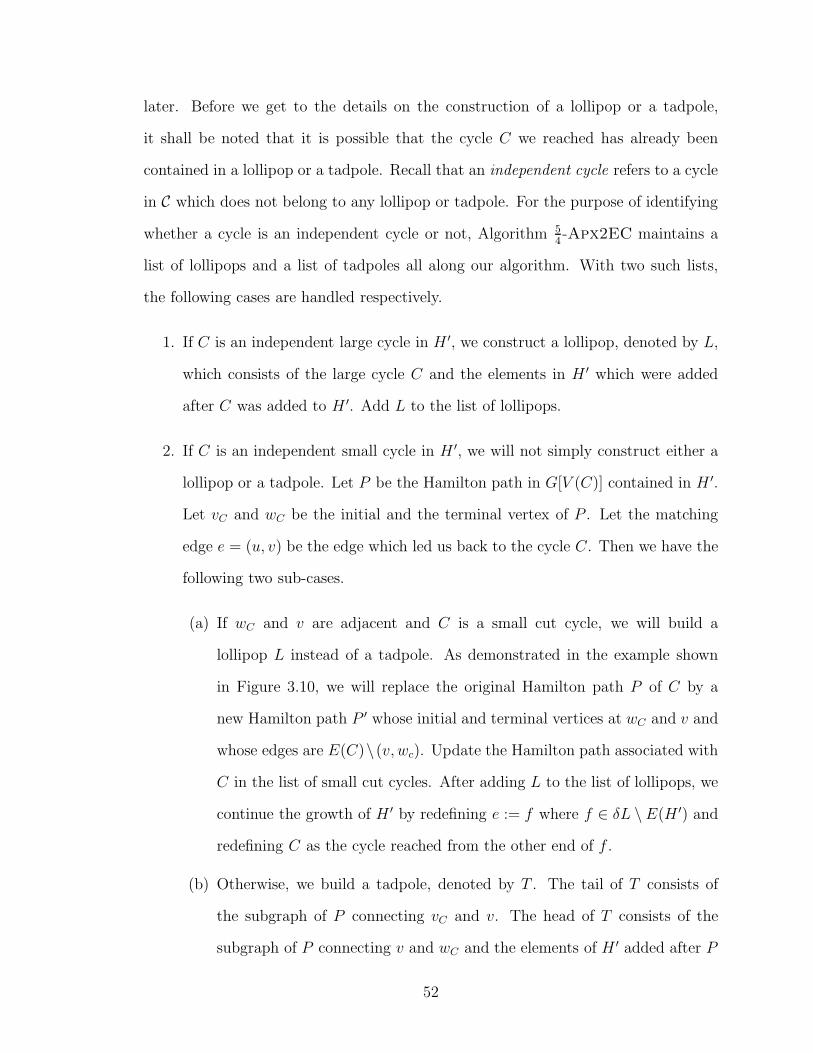
2EC for cubic graphs with 2-edge cuts. In section 3.3, we show it is possible to over-

come these problems and obtain a 54-approximation. We present a 5

4-approximation

algorithm for 2EC on any bridgeless cubic graphs. The previous best approximation

ratio known for 2EC for this class of graph was 54

+ ǫ for any ǫ > 0, given by Csaba,

Karpinski and Krysta.

Following the 54-approximation algorithm demonstrated in Section 3.3 for bridge-

less cubic graphs, we prove that the integrality gap of the LP relaxation for 2EC on

bridgeless cubic graphs is at most 54.

Given below are some common definitions widely used in this chapter.

36

Definition Recall that in a graph G = (V,E), a Hamilton path is a path in G that

covers all vertices in G; whereas a Hamilton cycle is a cycle that contains all vertices

in G. For a Hamilton path, its two ends are referred to as the initial vertex and the

terminal vertex respectively. A chord of a cycle C in a graph G = (V,E) is an edge

in E \ E(C), where both of its ends lie on C.

3.1 Review of a 6/5-approximation Algorithm for

2EC on Cubic 3-edge-connected Graphs [BIT13]

Taking a cubic 3-edge-connected graph G with n vertices as an input, S. Boyd, S.

Iwata and K. Takazawa designed an approximation algorithm for 2EC on G with a

performance guarantee of 65n, which is referred to as Algorithm Apx2EC. In this

section, we present a detailed review on this algorithm prior to the introduction of

our 54-approximation algorithm adapted from Apx2EC for solving 2EC on bridgeless

cubic graphs, i.e. cubic 2-edge-connected graphs.

For a cubic 3-edge-connected graph G = (V,E) with n vertices, the first step of

Algorithm Apx2EC is to use an algorithm called 34Cut [BIT13] to obtain a 2-factor

F of G covering all the 3- and 4-edge cuts. Note that a 2-factor F of a graph G that

covers all 3-edge cuts in G includes a pair of edges of every 3-edge cut in one of the

cycles of F . That is to say, such a 2-factor of any bridgeless cubic graph does not

contain any cycle consisting of three vertices, i.e. triangles. A 2-factor F of a graph

G that covers all 4-edge cuts in G contains a pair of edges of every 4-edge cut in

one of the cycles of F and the other pair of edges in a different cycle of F . This

suggests such a 2-factor of any 3-edge-connected cubic graph does not contain any

cycle consisting of 4 vertices, i.e. squares. Theorem 3.1.1[BIT13] proves that such a

2-factor exists in any bridgeless cubic graphs.

Theorem 3.1.1 (Theorem 5.4 [BIT13]). Given any bridgeless cubic graph G, Al-

37

gorithm 34Cut finds a 2-factor in G covering all the 3- and 4-edge cuts and not

containing a specified edge e∗ ∈ E in O(n3) time.

The edges in E \ F are called the matching edges. Since G is 3-edge-connected,

which means it does not contain any 2-edge cut, the structures shown in Figure 3.1

(a) and (b) do not exist in G. Moreover, with all 3- and 4-edge cuts covered, triangles

and squares obtained from the structures shown in Figure 3.1 (c) and (d) are avoided

in F . Therefore any cycle in F must contain at least 5 vertices. Denote the family of

(a) (b) (c) (d)

({e1, e2} and {e3, e4} are 2−edge−cuts)

e1

e2

e3

e4

Figure 3.1: Eliminated structures in Algorithm Apx2EC.

cycles in F by C, if any cycle C ∈ C contains at most 9 vertices, C is called a small

cycle, otherwise it is called a large cycle. Observe that all small cycles C have at

most two chords in G[V (C)] unless C contains all vertices in G, otherwise δ(V (C))

is a 3- or 4-edge cut covered by F . With Lemma 3.1.2 below applied, this first step

guarantees that any small cycle in F is traversable by a Hamilton path starting with

any vertex that is not incident to any chord and terminating at another vertex which

is also not incident to any chord.

Lemma 3.1.2 (Lemma 6.1 [BIT13]). Let G = (V,E) be a 2-edge-connected graph and

C be a cycle in G with at most two chords. Let V ∗ ⊆ V (C) be the set of vertices not

incident with the chords. For a vertex v∗ ∈ V ∗, there is a Hamilton path in G[V (C)]

starting at v∗ and ending at some vertex u∗ ∈ V ∗.

With a 2-edge-connected subgraph H with the property |E(H)| ≤ 65|V (H)| main-

tained all through the algorithm, the construction of the 2-edge-connected spanning

38

subgraph of G starts with initializing H with an arbitrary cycle C0 ∈ C, and ter-

minates when V (H) = V , which is the result of a series of expansion operations

in which H is augmented by adding another subgraph H ′. Every expansion starts

with choosing an arbitrary matching edge e = (u, v) ∈ δ(H), where u ∈ V (H) and

v ∈ V \ V (H), and initializing H ′ := (u, ∅). Let C ∈ C denotes the cycle containing

v. Note that initially C is not contained in H . Given e = (u, v) and C, repeat the

following different procedures for enlarging H ′ apply according to the following four

cases until v ∈ H is reached. Once v ∈ H is reached, the current expansion is finished

and H is augmented by H ′ and e, i.e., H := (V (H) ∪ V (H ′), E(H) ∪ E(H ′) ∪ {e}).

Case 1. If C is a large cycle that is not contained in H ′ yet, e and C are added to

H ′. Let f ∈ δ(H ′) \ e and let Cnew be the cycle containing the other end of f .

Update e := f and C := Cnew.

Case 2. If C is a small cycle that is not contained in H ′ yet, edge e and the Hamilton

path P of G[(V )], that starts at v and ends at some other vertex w which is not

incident to any chord, are added to H ′. The existence of such a Hamilton path

is proved by Lemma 3.1.2. We refer to the matching edge which is incident to

w as the leaving edge of P . Update e to be the leaving edge (w, z) ∈ δ(C), and

C to be the cycle containing z.

Case 3. If C is a large cycle that has already been included in H ′, a lollipop L,

which is defined as “a subgraph consisting of the large cycle C and the elements

of H’ added after C was added to H ′” [BIT13], is constructed, see Figure 3.2

for an illustration. It is followed by updates to both edge e and cycle C, as

e := f ∈ δ(L) \ E(H ′) and C := Cnew, where Cnew is the cycle containing the

other end of f .

Case 4. If C is a small cycle that has already been included in H ′, a tadpole, which is

defined as “a subgraph consisting of the Hamilton path P derived from C plus

39

the elements of H ′ added after P was added to H ′” [BIT13], is constructed,

see Figure 3.3 for an illustration. Let vC and wC be the initial and terminal

vertices of P . The head of a tadpole T “consists of the subgraph of P connecting

v and wC , and the elements of T added to H ′ after P was added to H ′”[BIT13];

while the tail of a tadpole H ′ is “a subgraph of P , the path connecting vC and

V ”[BIT13]. The growth of H ′ is continued from a matching edge connecting

the head of T to V \ V (T ). The existence of such a matching edge is proved in

the Lemma 3.1.3 [BIT13].

Lemma 3.1.3 (Lemma 6.2 [BIT13]). For Case 4, there exists an edge con-

necting the head of the tadpole T and V \ V (T ).

Proof. Suppose, for contradiction, there is no edge connecting the head of the

tadpole T and V \ V (T ). Let C ∈ C be the cycle that provides the tail of T .

It follows from the assumption that there is no edge between V \ V (T ) and

V (T ) \ V (C). Given that G is a 3-edge-connected cubic graph and the 2-factor

F of G resulted from Algorithm 34Cut covers all 3- and 4-edge cuts, therefore

there are at least five matching edges between V (C) and V \ V (T ) and at least

another five matching edges between V (C) and V (T ) \ V (C). It follows that

C contains at least 10 vertices, which contradicts the fact that C is a small

cycle.

Note that in the Case 3 and Case 4, it is possible that C is already included in a

lollipop or a tadpole in H ′. In this algorithm, a cycle in C which does not belong

to any lollipop and tadpole is referred to as an independent cycle [BIT13]. If C is

neither in H nor independent, a larger lollipop L is constructed if C is contained in a

lollipop L, which consists of L and all the elements of H ′ added after the construction

of L; while a larger tadpole T is constructed if C is contained in a tadpole T .

40

H C

Figure 3.2: Construction of a lollipop L. The thick edges are the edges in L. Thehexagon is a small cycle of size 6, and the four circles indicate large cycles. (Somevertices and edges are omitted.) (Fig. 6.1. [BIT13]).

H C

wC

v

vC

Figure 3.3: Construction of a tadpole T . The thick edges are the edges in T . Thehexagon is a small cycle of size 6, and the four circles indicate large cycles. (Somevertices and edges are omitted.) The thick edges connecting vc and v form the tail ofT , and other thick edges form the head of T . (Fig. 6.2. [BIT13]).

41

Since in Algorithm Apx2EC, only inclusion-wise maximal lollipops and tadpoles

are handled, a list of lollipops and tadpoles is kept along the process of constructing

the 2-edge-connected spanning subgraph. Whenever a larger lollipop L (or a larger

tadpole T ) is built, all lollipops and tadpoles contained in L (or T ) are removed from

the list.

Theorem 3.1.4 (Lemma 6.4 [BIT13]). Algorithm Apx2EC is a 65-approximation

algorithm for 2EC in 3-edge-connected cubic graphs. More precisely, for a 3-edge-

connected cubic graph G = (V,E), Algorithm Apx2EC finds a 2-edge-connected sub-

graph H of G with E(H) ≤ 65n− 1 in O(n3) time.

Corollary 3.1.5 (Corollary 6.5 [BIT13]). For a 3-edge-connected cubic graph G =

(V,E) and two adjacent edges e1, e2 ∈ E, one can find a 2-edge-connected subgraph

H of G with E(H) ≤ 65n− 1 and {e1, e2} ⊆ E(H) in O(n3) time.

From Theorem 3.1.4 and Corollary 3.1.5, it follows that Algorithm Apx2EC pro-

duces a 2-edge-connected spanning subgraph for 3-edge-connected cubic graphs with

no more than 65n− 1 edges, which contains a specified pair of adjacent edges.

3.2 Why Apx2EC Does Not Work for Bridgeless

Cubic Graphs

With the knowledge that Algorithm Apx2EC only applies to 3-edge-connected cubic

graphs, we investigate the problems encountered when applying Apx2EC to bridge-

less cubic graphs, i.e., 2-edge-connected cubic graphs.

An obvious difference between 3-edge-connected cubic graphs and bridgeless cubic

graphs is that there exist 2-edge cuts in the latter. For any bridgeless cubic graph

G = (V,E), after Algorithm 34Cut is applied to G, the existence of the 2-edge cuts

in G may lead to the follow two problems.

42

1. Existence of small cut cycles in C.

Recall that C is used to denote the family of cycles in the 2-factor F , where

F is the result of applying Algorithm 34Cut to G. A cycle C ⊂ C is referred

to as a cut cycle if the removal of C leaves the rest of G with more than one

component. More precisely, for any cycle C ⊂ C, if G−G[V (C)] has more than

one component, C is considered as a cut cycle. Figure 3.4 illustrates an example

of a small cut cycle that contains 6 vertices and 1 chord.

e1

A

v1

v2e2

v3

v5

C

e3

e4

v4

v6

B

Figure 3.4: A small cut cycle C of size 6, whose removal separate the graph intotwo components A and B, where B is a large cycle with 10 vertices.

The problem with cut cycles for graphs with 2-edge cuts arises when a cut cycle

in C ∈ C is a small one. The proof of Lemma 3.1.3 depends on the fact that all

cuts arising from a cut cycle must have size at least 5 (i.e. contain at least five

edges), and thus no small cycle can be a cut cycle in a 3-edge-connected graph

in Algorithm Apx2EC. However, if G is only 2-edge-connected, small cut cycles

can exist, which may invalidate Lemma 3.1.3 and the construction process of

some subgraph H ′. Consider Figure 3.4 as an example, in which C is a small

cut cycle with 6 vertices whose removal disconnects G into two components, A

and B. Suppose A is H , after edge e1 is chosen to start the construction of H ′,

Algorithm Apx2EC chooses “v1−v2−v3−v4−v5−v6” as the Hamilton path

to traverse the small cut cycle C that consists of six vertices, and continues the

construction of H ′ from the matching edge e3. Denote the cycle reached from

e3 by CB. Since CB contains 10 vertices, which means CB is considered as a

43

large cycle, it will be added into H ′ according to Case 1 in Algorithm Apx2EC.

At this point, e4 becomes the only choice to continue the construction of H ′,

from which C is reached again. It follows with the construction of a tadpole T

with its head shown with thick solid edges and its tail shown with thick dotted

edges. It becomes easy to see that there does not exist any edge connecting the

head of T and V \ V (T ). In this case, Algorithm Apx2EC cannot be applied.

2. Existence of 4-cycles in C

The existence of 2-edge cuts in a bridgeless cubic graph G may also lead to the

existence of 4-cycles in C, which is the family of cycles in a 2-factor covering

all 3- and 4-edge cuts in G, which is avoided in Algorithm Apx2EC with all

4-edge cuts covered. However, with 2-edge cuts existing in G, the existence of

structures shown in Figure 3.1 (a) and (b) becomes possible. The structure

shown in Figure 3.1 (a), which is referred to as a diamond structure, may lead

to a 4-cycle in C, while the structure shown in Figure 3.1 (b), which is a 4-cycle

joined by two 2-edge cuts, may not only cause a 4-cycle but may also cause a

small cut cycle in C. Note that a diamond structure contains a cycle of four

vertices with one chord, and the two matching edges in δ(V (C)) form a 2-edge

cut.

The reason that we are concerned about the existence of 4-cycles is that in the

proof for Theorem 3.1.4, the definition of small and large cycles was applied to

obtain the relationship between numbers of small cycles as well as large cycles

in C and the number of vertices in the input 3-edge-connected cubic graph

G = (V,E), i.e. |V | ≥ 5|S|+10|L|, where S ⊆ C denotes the set of small cycles

and L ⊆ C denotes the set of large cycles. However, this relationship does not

apply any longer with the existence of 4-cycles, and thus the definition of small

cycles is required to be modified.

44

Figure 3.5: A bridgeless cubic graph G illustrating that it is not always possible to finda 2-factor that covers all 2-edge cuts.There are three 2-edge cuts in G, while only two ofthem can be covered by any 2-factor of G to a maximum extent.

Considering the above two problems in applying Algorithm Apx2EC to bridgeless

cubic graphs, as well as the fact that it is not always possible to find a 2-factor that

covers all 2-edge cuts (see Figure 3.5 for a counter example), in extending Algorithm

Apx2EC to bridgeless cubic graphs, the concept of small cycles and large cycles is

redefined to compromise with 4-cycles, and two new strategies are applied during

the construction of tadpoles to make our algorithm compatible with the existence of

small cut cycles. With these ideas realized, we present a 54-approximation algorithm

for 2EC on bridgeless cubic graphs in the upcoming section.

3.3 A 5/4-approximation Algorithm for 2EC on Bridge-

less Cubic Graphs

As inspired by Algorithm Apx2EC[BIT13], the general idea of our algorithm for 2EC

on a bridgeless cubic graph G = (V,E) is also to build the 2-edge-connected spanning

subgraph of G based on a 2-factor of the graph G covering all 3- and 4-edge cuts

obtained by Algorithm 34Cut [BIT13], which applies to all bridgeless cubic graphs.

As before, we use F to denote the 2-factor of G that covers all 3- and 4-edge cuts

obtained from Algorithm 34Cut [BIT13], and C is used to denote the family of cycles

in F . Note that since F covers all 3-edge cuts in G, it follows that triangles do not

45

exist in C, and also considering that loops and parallel edges are not considered in

this chapter, the minimum-possible cycles in C contain 4 vertices.

In order to solve the two problems stated in Section 3.2, the following modifications

are applied in the design of our algorithm, which is referred to as 54-Apx2EC.

Change 1. In Algorithm 54-Apx2EC, a cycle C ⊂ C is referred to as a small cycle

if 4 ≤ |V (C)| ≤ 7; and it is called as a large cycle if |V (C)| ≥ 8.

Change 2. When a small cut cycle is first encountered during the construction of

some subgraph H ′, certain constraints for selecting a proper Hamilton path for

a certain initial vertex are added in Algorithm 54-Apx2EC.

Change 3. When a small cut cycle C ∈ C is reached again during the construction

of some subgraph H ′, instead of certainly building a tadpole as in Algorithm

Apx2EC, Algorithm 54-Apx2EC may choose to build a lollipop rather than a

tadpole if the vertex, from which the small cycle is reached again, is incident to

the terminal vertex of the Hamilton path of G[V (C)] in the subgraph H ′ under

construction.

With a 2-factor obtained which covers all the 3- and 4-edge cuts while excluding a

specified edge e∗ ∈ E, the construction of the 2-edge-connected spanning subgraph

in Algorithm 54-Apx2EC starts with an arbitrary cycle C0 ∈ C. During the whole

process, we maintain a subgraph H satisfying the following properties:

1. H is 2-edge-connected;

2. V(H) is the union of the vertex set of a subfamily of the cycles in C;

3. |E(H)| ≤ 54|V (H)|.

Initially, let H := C0, and then H is repeatedly augmented by adding another

subgraph H ′. Algorithm 54-Apx2EC terminates when V (H) = V .

We start to build H ′ by initializing H ′ := (u, ∅), where u ∈ V (H) is an arbitrary

vertex on H . Since G is a cubic graph, there exists an edge e = uv ∈ δ(H), where

46

u ∈ V (H) is the arbitrary vertex we chose to initialize H ′ and v ∈ V \ V (H).

Apparently, v belongs to a cycle, denoted by C, where C ⊂ C is not contained in H .

At this point, according to whether C is a large cycle or a small one, we handle C

differently.

1. C is A Large Cycle.

If C is a large cycle, then we add e and C into H ′, i.e. we let H ′ := (V (H ′) ∪

V (C), V (H ′) ∪ e ∪ E(C)). Afterwards, redefine e := f , where f is an arbitrary

matching edge other than e ∈ δ(C), and redefine C as the cycle we reach at the

other end of f . We continue to grow H ′ from the newly-defined e and C.

2. C is A Small Cycle.

If C is a small cycle, things become more complicated. With the definition for

small cycles and large cycles modified, it becomes necessary to verify whether

Lemma 3.1.2 still applies for any small cycle C ∈ C such that a Hamilton path

does exist in G[V (C)] starting at any vertex on C.

Lemma 3.3.1. For any small cycle C ∈ C, C has at most two chords.

Proof. Following the definition of small cycles, a small cycle C ∈ C can only be

of size 4, 5, 6 and 7.

If |V (C)| = 4, C can have at most one chord, otherwise G is not connected.

If |V (C)| = 5, C cannot have any chord, otherwise either F doesn’t cover a

3-edge cut or G has a cut cycle.

If |V (C)| = 6, C can have at most two chords, otherwise G is not connected.

If |V (C)| = 7, C can have at most one chord, otherwise either F doesn’t cover

a 3-edge cut or G has a cut edge.

In conclusion, any small cycle C ∈ C can have at most two chords.

Lemma 3.3.1 implies that any small cycle in a 2-factor covering all 3- and 4-edge

cuts in graph G has at most two chords. According to Lemma 3.1.2[BIT13],

47

for any small cycle C in the 2-factor F of G, no matter from which vertex v we

enter the cycle C, there is always a Hamilton path of G[V (C)] that takes v as

the initial vertex and terminates at a vertex incident to no chord.

With the existence of such a Hamilton path of G[V (C)] proved, different oper-

ations are applied to C, which is a small cycle, depending on whether C is a

cut cycle or not.

If C is not a cut cycle, an arbitrary Hamilton path P of G[V (C)], that takes v

as the initial vertex and terminates at some vertex not incident to any chord, is

chosen. Suppose the terminal vertex of P is w, and the matching edge incident

to w is f . Add e and P into H ′, and continue the growth of H ′ using e := f

and using the cycle containing the other end of f as C.

If C is a cut cycle, instead of choosing any Hamilton cycle starting from v and

ending at a vertex incident to no chord, it becomes necessary to select a certain

Hamilton cycle if multiple options do exist, which is the second modification

stated above. For this purpose, concepts of backward edges and forward edges

are introduced concerning a small cut cycle, denoted by CScut. Let the component

in G − CScut that contains C0 be denoted by SB, while the rest of G − CS

cut is

denoted as SF . An edge e ∈ δ(CScut) is labeled as a backward edge if e has exactly

one end in CScut and the other end in SB, and a forward edge if e has exactly one

end in CScut and the other end in SF . Lemma 3.3.2 below proves some important

characteristics of a small cut cycle in CScut ∈ C.

Lemma 3.3.2. A small cut cycle C ∈ C has the following properties:

(a) G− C consists of either 2 or 3 components;

(b) |V (C)| = 7 or |V (C)| = 6 or |V (C)| = 4;

(c) Only when |V (C)| = 6, C can have one chord, otherwise, C has no chord.

(d) The number of forwarded edges for C is 2 or 4 or 5.

48

Proof. Since G is 2-edge-connected and F covers all the 3- and 4-edge cuts, each

component in G− C is connected to C by either 2 edges or at least 5 edges in

G.

As C is a small cycle where |V (C)| ≤ 7, the number of components in G − C

is at most 3. Considering C is also a cut cycle, the number of components in

G − C is either 2 or 3. Next, we list all possible conditions for such a small

cycle in G.

• 7-cycles:

Figure 3.6: A cut cycle of order 7 (Case I).

When |V (C)| = 7, G−C can only have 2 components and no chord. The

number of the forwarded edges is either 2 or 5. (As shown in Figure 3.6)

• 6-cycles:

Figure 3.7: A cut cycle of order 6 with no chord (Case II)

When |V (C)| = 6 and C has no chord, G − C has 3 components. The

number of its forwarded edges is either 2 or 4. (As shown in Figure 3.7)

49

Figure 3.8: A cut cycle of order 6 with one chord (Case III).

When |V (C)| = 6 and C has one chord, G − C has 2 components. The

number of the forwarded edges is 2. (As shown in Figure 3.8)

• 5-cycles:

Since the 2-factor F we obtained in Step 1 covers all 3- and 4-edge cuts,

a cycle with the order of 5 cannot be a cut cycle. Otherwise G will have a

cut edge, which contradicts the fact that G is a bridgeless cubic graph.

• 4-cycles:

Figure 3.9: A cut cycle of order 4 (Case IV).

When |V (C)| = 4, G−C can only have 2 components and no chord. The

number of its forwarded edges is 2. (As shown in Figure 3.9)

In Conclusion, Lemma 3.3.2 is proved.

With the knowledge of Lemma 3.3.2, a Hamilton path on G[V (C)] when C is

a small cut cycle is chosen in the following way. If there is only one Hamilton

path of G[V (C)] that starts at v and ends at a vertex not incident to any

chord, this particular Hamilton path, which is referred to as P , is selected.

Let w denote terminal vertex of P , and f is used to denote the matching edge

50

incident to w. Otherwise, if multiple choices do exist for such a Hamilton path,

the chosen Hamilton path P must be selected as follows. If there is a Hamilton

path P whose leaving edge is a backward edge, this Hamilton path P with a

backward leaving edge is chosen. Otherwise, we will choose the Hamilton path

P of G[V (C)] whose leaving edge is the closest to a backward edge of C other

than e.

With the Hamilton path P chosen, let H ′ := (V (H ′)∪V (C), E(H ′)∪e∪E(P )),

and continue the growth of H ′ with the leaving edge f of P . Redefine e := f

and C as the cycle containing the other end of f .

Note that in order to identify a small cut cycle in linear time, a list of small cut

cycles is generated once the 2-factor F is obtained. This can be done simply by

temporarily removing every small cycle and see whether its removal disconnects

the graph G. For each small cut cycle in the list, the Hamilton path chosen for

it is recorded and maintained in the list as well.

We shall only face the above two situations at the very beginning of the construc-

tion of H ′. More accurately, the above two procedures are only applied when C is

not contained in H or H ′.

If we reach a cycle C which is already contained in H , the growth of H ′ is com-

pleted and we augment H with H ′, i.e. H := (V (H) ∪ V (H ′), E(H) ∪E(H ′) ∪ {e}).

After this, we will check whether the equation V (H) = V holds. If it holds, which

means we have a subgraph which covers all vertices in G and has the property of 2-

edge-connectivity, the algorithm terminates. Otherwise, we start to construct a new

H ′ from an arbitrary edge e ∈ δ(H) all over again.

If we reach a cycle C which is already contained in H ′, we need to build either a

lollipop or a tadpole, which are already defined in Section 3.1. Similarly, a lollipop is

built if C is a large cycle while a tadpole is constructed if C is a small cycle. However,

special strategies apply when C is a small cut cycle, which will be discussed in detail

51

later. Before we get to the details on the construction of a lollipop or a tadpole,

it shall be noted that it is possible that the cycle C we reached has already been

contained in a lollipop or a tadpole. Recall that an independent cycle refers to a cycle

in C which does not belong to any lollipop or tadpole. For the purpose of identifying

whether a cycle is an independent cycle or not, Algorithm 54-Apx2EC maintains a

list of lollipops and a list of tadpoles all along our algorithm. With two such lists,

the following cases are handled respectively.

1. If C is an independent large cycle in H ′, we construct a lollipop, denoted by L,

which consists of the large cycle C and the elements in H ′ which were added

after C was added to H ′. Add L to the list of lollipops.

2. If C is an independent small cycle in H ′, we will not simply construct either a

lollipop or a tadpole. Let P be the Hamilton path in G[V (C)] contained in H ′.

Let vC and wC be the initial and the terminal vertex of P . Let the matching

edge e = (u, v) be the edge which led us back to the cycle C. Then we have the

following two sub-cases.

(a) If wC and v are adjacent and C is a small cut cycle, we will build a

lollipop L instead of a tadpole. As demonstrated in the example shown

in Figure 3.10, we will replace the original Hamilton path P of C by a

new Hamilton path P ′ whose initial and terminal vertices at wC and v and

whose edges are E(C)\(v, wc). Update the Hamilton path associated with

C in the list of small cut cycles. After adding L to the list of lollipops, we

continue the growth of H ′ by redefining e := f where f ∈ δL \E(H ′) and

redefining C as the cycle reached from the other end of f .

(b) Otherwise, we build a tadpole, denoted by T . The tail of T consists of

the subgraph of P connecting vC and v. The head of T consists of the

subgraph of P connecting v and wC and the elements of H ′ added after P

52

Figure 3.10: Construct a lollipop L when returning back to an independent smallcycle C from an adjacent vertex v to the terminal vertex wc of the original Hamiltonpath in C, as explained in Case 2(a). The thick dotted edges in (a) are edges in theoriginal Hamilton path on C, while the thick dotted edges in (b) are edges in themodified Hamilton path on C. All thick edges in (c) are edges in the lollipop.

53

was added to H ′. Add T to the list of tadpoles.

3. If C is not independent and contained in a lollipop, say L, in H ′, we construct

a larger lollipop denoted by L, where L consists of L and all the elements in

H ′ which were added after L was built. Delete L from the list of lollipops, and

add L to the list of lollipops.

4. If C is contained in a tadpole, say T , we have the following two sub-cases

depending on whether C is a small cut cycle or not.

(a) C satisfies the following three conditions: (1) C is a small cut cycle; (2) v

is adjacent to wC; and (3) part of P , as the Hamilton path on G[V(C)], is

the tail of T . In this case, we modify T into a lollipop L. This will be done

by replacing P by a different Hamilton path P ′ whose initial and terminal

vertices are v and wC and whose edges are the edges of E(C) \ (v, wc).

Figure 3.11 shows an example of the transformation. Update the Hamilton

path associated with the small cut cycle C in the list of small cut cycles.

Delete T from the list of tadpoles and add L to the list of lollipops. Note

that we proved case-by-case that this situation is not possible to exist in

our algorithm with the restriction on the size of small cycles. However,

in order to complete this algorithm and, more importantly, to leave the

chance to improve or generalize our algorithm, the method for dealing

with this situation is still documented here. Also, the example shown in

Figure 3.11 is only for the purpose of illustration and is not possible to

appear in the process of Algorithm 54-Apx2EC.

(b) If C does not satisfy the three conditions from (a), we construct a larger

tadpole T , consisting of T and all elements in H ′ added after T was added.

If vertex v ∈ V (C) belongs to the tail of T , the tail T is the subgraph of

P connecting vC and v, and the head is the rest of T without the edges

54

Figure 3.11: Transform a tadpole to a lollipop when returning back to a small cycleC that satisfies all three conditions presented in Case 4(a). The thick edges in (a) areedges in the original tadpole T , while the thick edges in (b) are edges in the lollipoptransferred from T .

55

in its tail. If vertex v ∈ V (C) belongs to the head of T , then the tail of

T remains the same as the tail of T and its head consists of the head of

T and the elements of H ′ which were added after the construction of T .

After removing T from the list of tadpoles, add T into the list of tadpoles.

After the above procedures, if we constructed a lollipop L, then we continue the

growth of H ′ by redefining e := f where f ∈ δ(L) \ E(H ′) and redefining C as

the cycle reached at the other end of f . On the contrary, if a tadpole was built, we

continue the growth of H ′ by redefining e := f where f is a matching edge connecting

the head of T to V \ V (T ) and redefining C as the cycle reached at the other end of

f .

Note that by maintaining the list of lollipops and the one of tadpoles, we can

ensure that we only deal with inclusion-wise maximal lollipops and tadpoles. This

ensures that whenever we reach a cycle which belongs to a lollipop or a tadpole, it

does not belong to any other lollipops or tadpoles.

Below we presents a more systematical description of the algorithm.

Algorithm 3.1. 54-Apx2EC

Input. a 2-edge-connected cubic graph G = (V,E) and two adjacent edge e1 and e2.

Output. a 2-edge-connected subgraph H of G that has at most 5|V |4

edges and

contains e1 and e2.

Step 1. Using Algorithm 34Cut to find a 2-factor F of G that covers all the 3- and

4-edge cuts but excludes the edge e3 = δ(x) \ {e1, e2}, where x is the common

vertex that e1 and e2 are both incident to. For every small cycle in F , add it to

the list of small cut cycles if its removal disconnects the graph G. Choose the

cycle C0 in F that contains e1 and e2, set H := C0, and then go to Step 2.

Step 2. If V (H) = V , then return H . Otherwise, choose an arbitrary edge e = uv ∈

V (H) and v ∈ V \V (H), and let H ′ be the graph consisting of the single vertex

56

u, and go to Step 3.

Step 3. Denote by C the cycle in F containing v. If C is not contained in H , then

go to Step 4. Otherwise, go to Step 5.

Step 4. Here we have the following cases.

Case 1. If C is a large cycle not contained in H ∪H ′, then go to Step 4-1.

Case 2. If C is a small cycle not contained in H ∪H ′, then go to Step 4-2.

Case 3. If C is an independent large cycle in H ′ or contained in a lollipop in

H ′, then go to Step 4-3.

Case 4. If C is an independent small cycle in H ′ or contained in a tadpole in

H ′, then go to Step 4-4.

Step 4.1. Add e and C to H ′. That is, set V (H ′) := V (H ′) ∪ V (C) and

E(H ′) := E(H ′)∪E(C)∪e. Then choose an arbitrary edge f from δ(C)\e,

set the vertex that is the end of f not in C to v, set e := f , and then go

to Step 3.

Step 4.2. (Modification 1)

If C is not a cut cycle, choose a Hamilton path of G[V (C)], starting at v

and ending at a vertex w not incident with a chord of C, denoted by P.

If C is a cut cycle and there is more than one such Hamilton path, then

choose the Hamilton path as follows. Let S be the vertex set of the compo-

nent of G−V (C) containing H . Label the two different sets of edges which

are connecting V (C) with S and V (C) with V \ (S∪C) as backward edges

and forward edges respectively. If among all the Hamilton cycles there

exists one whose leaving edge is a backward edge, then choose this one as

P . Otherwise, choose the Hamilton path whose leaving edge is closest to

57

a backward edge. Define the Hamilton path associated with C in the list

of small cut cycles as P .

Add e and P to H’, that is, set V (H ′) := V (H ′) ∪ V (C) and E(H ′) :=

E(H ′) ∪ E(C) ∪ e. Then let f be the matching edge incident with w, set

the vertex that is the other end of f to v, set e := f , and then go to Step

3.

Step 4.3. Add e to H ′ and construct a lollipop L. Remove any lollipops or

tadpoles contained in L from the list of lollipops and tadpoles. Then

choose an arbitrary edge f from δ(L) \ E(H ′), set the vertex that is the

end of f not in L to v, set e := f , and then go to Step 3.

Step 4.4. (Modification 2)

If C is one of the following conditions:

(a). C is not a cut cycle;

(b). C is an independent cut cycle and v is not adjacent to the terminal

vertex of the Hamilton path P of G[V (C)];

(c). C is a cut cycle which is completely contained in the head of some

tadpole; or

(d). C is a cut cycle in which part of the Hamilton path P of G[V (C)]

forms the tail of some tadpole, but v is not adjacent to the terminal

vertex of P .

Add e to H ′ and construct a tadpole T. Remove any lollipops or tadpoles

that are contained in T from the list of lollipops and tadpoles. Then,

choose an arbitrary edge f connecting the head of T to V V (T ), set the

vertex that is the end of f not in T to v, set e := f , and go to Step 3.

If C does not satisfy the above conditions, C is a small cut cycle, that

is reached again from v which is adjacent to the terminal vertex wc of

58

the Hamilton path P of G[V (C)], which will form the tail of a tadpole.

Replace P on G[V (C)] with a new Hamilton path whose initial vertex and

terminal vertex are v and wc and whose edges are E(C) \ (v, wc). Update

the Hamilton path P associated with C in the list of small cut cycles. By

doing this, instead of a tadpole, a lollipop L is constructed and thus added

to H ′ along with e. Then, choose an arbitrary edge f from δ(L) \ E(H ′),

set the vertex that is the end of f not in L to v, set e := f , and go to Step

3.

Step 5. Augment H by H ′ and e. That is, set V (H) := V (H)∪V (H ′) and E(H) :=

E(H) ∪ E(H ′) ∪ e. Then go to Step 2.

Before we finished the algorithm completely, there is still one point remaining

to be proved. One may question that after the construction of a tadpole T in the

algorithm, is there another edge connecting the head of the tadpole T to V \ V (T )?

Because if such an edge does not exist, any edge belonging to the tail of T can be

a cut edge for the solution, in which case our solution will not be 2-edge-connected.

Lemma 3.3.3 presented below solves this question with no doubt.

Lemma 3.3.3. For a tadpole T , there exists an edge connecting the head of the tadpole

T and V \ V (T ).

Proof. Suppose, to the contrary, that there exists no edge connecting the head of a

tadpole T and V \V (T ). Denote the small cycle providing the tail of T by CT , which

must be a small cut cycle. Denote the chosen Hamilton path of G[CT ] by P , and the

matching edge used to come to CT the first time by mT = (u, v), where u ∈ V (CT ).

Denote the component in G−CT containing the initial cycle C0 by H0, and the other

part by H1. Note that G − CT has only two components (as both H0 and H1 are

connected).

59

We can prove this lemma considering the following different cases, which are in

accordance with the four cases presented in the previous proof for Lemma 3.3.2.

Case I: |V (C)| = 7, G− C can only have 2 components and no chord.

Case II: |V (C)| = 6 and C has no chord, G− C has 3 components.

Case III: |V (C)| = 6 and C has one chord, G− C has 2 components.

Case IV: |V (C)| = 4, G− C can only have 2 components and no chord.

• For Case II

As G− CT has only two components, this case is eliminated.

• For Cases I and IV

Denote the forward edge which is used to leave CT by (wc, wx) and the forward

edge which is used to come back to CT by (u, v), where wc, v ∈ V (CT ) and

wx, u ∈ V (H1). According to Step 4-4 in our algorithm, there must be at least

one vertex between wc and v on P ; otherwise we form a lollipop, not a tadpole,

according to Modification 2. Let p denote one such vertex.

Since C has no chord in Cases I and IV, p must be incident with a forward edge

(otherwise we have an edge from the head of T to V \ V (T )). Also, C consists

of the Hamilton path P plus edge (v0, wc), where v0 is the node where we first

enter C in the algorithm.

Thus there exist at least two vertices on P between (wc, wx) and a backward

edge. According to Step 4-2, the matching edges incident with three vertices

closest to v on P are forward edges. Therefore, CT has at least six forward

edges, which eliminates Cases I and IV.

• For Case III

For Case III, where we have one chord in the 6-cycle, there are six possibilities

for the set of forward and backward edges, as shown in Figure 3.12.

60

(f)

(a) (b) (c)

(e)(d)

Figure 3.12: Six combinations of backward (dashed) and forward (solid) edges in a6-cycle with one chord.

1

2

3

1

3

2

3

3

1

3

2

2

3

1

3

thin dashed curve with solid arrow − backward edge which enters the current cycle C

thick dashed curve with no arrow − backward edge which connects the head of the tadpole T to V\V(T)

thick dotted curve with hollow arrows − forward edges

thin solid line with solid arrow − edge on the Hamilton path which belongs to the tail of the tadpole

thick dotted line with solid arrow − edge on the Hamilton path which belongs to the head of the tadpole

(c)(b)(a)

Figure 3.13: Different layout of backward edges and forward edges for Figure 3.12(e) and (f).

61

For Figures 3.12 (a), (b), (c) and (d), it is clear that no matter from which

backward matching edge of the two we entered the cycle, i.e. the first backward

edge, we will always have a Hamilton path in which the leaving edge is also

a backward edge. Thus, according to Modification 1, we choose the Hamilton

path which ends with a backward leaving edge, and the cycle will not be a

tadpole.

For Figure 3.12 (e) and (f), no matter from which backward edge we entered, we

will get out with a Hamilton path with a leaving forward edge. After we come

back from another forward edge, it will form a tadpole. However, the head of

the tadpole contains a vertex which is incident to the unused backward edge.

See Figure 3.13. Note that the other possibility for (c) in Figure 3.13 does not

occur because of Step 4.2, in which a Hamilton path whose leaving edge is the

closest to a backward edge is chosen. Hence there exists an edge connecting the

head of the tadpole T and V (T ).

In conclusion, we have Lemma 3.3.3 is proved.

Lemma 3.3.4. For an output H of Algorithm 3.1, it holds that |E(H)| ≤ 54n− 1.

Proof. For n ≤ 7, the initial 2-factor which covers all the 3- and 4-edge cuts must

consist of just one cycle and thus |E(H)| = n.

For n ≥ 8, partition the family C of cycles in F into two sub-families, L and S, where

L is the family of large cycles, while S is that of small cycles. By construction, it

is clear that H contains at most 2(|C| − 1) edges from the matching edges E \ F .

Moreover, we use |C| edges from G[(V )] where C ∈ L, and (|C|−1) edges from G[(V )]

where C ∈ S, except possibly the initial cycle C0. If the initial cycle C0 is a small

cycle, then |C| edges from C0 will be used. Thus, using |F | = n, it follows that:

|E(H)| ≤ n− (|S| − 1) + 2(|S| + |L| − 1) = n+ |S| + 2|L| − 1 ≤5

4n− 1 (3.1)

62

Note that the last inequality holds because we took small cycles starting from 4 and

large cycles starting from 8, hence n ≥ 4|S| + 8|L|, which means, |S| + 2|L| ≤ 14n.

It follows that |E(H)| ≤ max{n, 54n − 1}. However, because for any cubic graphs,

n ≥ 4, which leads to n ≤ 54n− 1. In conclusion, |E(H)| ≤ 5

4n− 1.

Corollary 3.3.5. For a 2-edge-connected cubic graph G = (V,E) and any two adja-

cent edges e1, e2 ∈ E, there exists a 2-edge-connected spanning subgraph H of G with

|E(H)| ≤ 54n− 1 and {e1, e2} ⊆ E(H) which can be found in O(n3) time.

Proof. Let e1, e2 ∈ E be adjacent at some vertex x ∈ V , and let e3 = δ(v) \ {e1, e2}.

It has been stated that the Algorithm 34Cut we applied at Step 1 can obtain a

2-factor in a 2-edge-connected cubic graph covering all the 3- and 4-edge cut in G

and not containing a certain edge e∗. Let e3 be the certain edge that we exclude from

the 2-factor we found in Step 1 using the algorithm 34Cut. It follows that e1 and

e2 must be contained in one of the cycles in F , say C∗. According to the Step 1 of

Algorithm 3.1, by choosing C∗ to be the initial cycle to start the algorithm, e1 and

e2 are certainly contained in the resulted spanning subgraph H .

Considering the complexity of Algorithm 3.1, we first give a list of differences

between Algorithm 3.1 and Algorithm Apx2EC as follows:

1. After a 2-factor F covering all 3- and 4-edge cuts in the graph G is obtained,

there is an additional operation in Step 1, which is to detect all small cut cycles

in the family of cycles in F . For the simplicity of the algorithm, this operation

can be done by temporarily removing the small cycle C under detection and see

whether the rest of G has more than one component. We have at most n4

small

cycles, and for each of them the checking procedure takes O(n2) in the worst

case. Hence this operation takes O(n3) in the worst case.

2. In Step 4.2, instead of choosing an arbitrary Hamilton path, we need to choose

a certain one if the underlying cycle is a small cut cycle. However, since the

63

number of Hamilton paths in a small cut cycle is constant, it would not change

the complexity of this step.

3. In Step 4.4, instead of building a tadpole, we only construct a tadpole if the

underlying cycle C can pass a verification procedure by satisfying the following

conditions:

(a). C is not a cut cycle;

(b). C is an independent cut cycle and v is not adjacent to the terminal

vertex of the Hamilton path P of G[V (C)];

(c). C is a cut cycle which is completely contained in the head of some

tadpole; and

(d). C is a cut cycle that part of the Hamilton path P of G[V (C)] forms the

tail of some tadpole, but v is not adjacent to the terminal vertex of P .

Otherwise, we construct a lollipop by updating the original Hamilton path on

C to a new one. This operation is completed in constant time, with the aid of

the list of small cut cycles where the associated Hamilton path for each of them

is maintained.

With a list of small cut cycles, including the information on their associated

Hamilton paths, a list of tadpoles and a list of lollipops maintained, the above

verification procedure is completed in linear time. And the rest of the procedure

for building a tadpole stays the same as that for Algorithm Apx2EC.

Given that the computational complexity for Algorithm Apx2EC is O(n3), it follows

from the above discussions that the computational complexity for Algorithm 3.1 is

also O(n3).

Hence Corollary 3.3.5 is proved.

Theorem 3.3.6. The integrality gap of 2EC is at most 54

for bridgeless cubic graphs.

64

Proof. From Lemma 3.3.4, it is known that for an output H of Algorithm 3.1, it holds

that |E(H)| ≤ 54n− 1, i.e.

OPT (G) ≤5

4n− 1.

The integrality gap of 2EC for bridgeless cubic graphs, denoted as α2EC(G), equals

the ratio between OPT (G) and OPTLP (G) for any bridgeless cubic graph G with any

cost function. Considering that for any bridgeless cubic graph G with n vertices,

OPTLP (G) ≥ n,

it follows that

α2EC(G) =OPT (G)

OPTLP (G)

≤5n/4 − 1

n

=5

4.

(3.2)

Hence the integrality gap of 2EC is at most 54

for bridgeless cubic graphs.

With Section 3.1 given as a fundamental introduction on Algorithm Apx2EC

[BIT13], which is the cornerstone of Algorithm 3.1 we presented in Sections 3.3,

we explained the problems of applying Algorithm 3.1 to obtain solution of 2EC on

bridgeless cubic graphs in Section 3.2. By giving methods to overcome the above

barriers, we gave a 54-approximation algorithm for bridgeless cubic graphs with the

computational complexity of O(n3). Furthermore, Algorithm 3.1 provides an upper

bound on the integrality gap of the LP relaxation on 2EC for bridgeless cubic graphs

as 54.

65

Chapter 4

Computational Study on the

Integrality Gap of 2EC

Having tried different approaches for designing an approximation algorithm with bet-

ter approximation ratios, special families of graphs with some structures, such as the

diamond structures, were found to cause a high ratio between OPT (G) and the num-

ber of vertices n for graphs G in such families. However, they do not necessarily cause

a high ratio between OPT (G) and OPTLP (G). This finding led to further studies

on the integrality gap of 2EC, which was the motivation for the computational study

presented in this chapter.

In this chapter, we investigate the worst-case ratio between ILP (G) and LP (G)

computationally for graphs with a small number of vertices. More specifically, we do

this for the following classes of graphs:

• All bridgeless graphs with k vertices, where 3 ≤ k ≤ 10.

• All bridgeless cubic graphs with k vertices, where 6 ≤ k ≤ 16.

• All bridgeless subcubic graphs with k vertices, where 3 ≤ k ≤ 16.

This chapter includes two sections representing the two major stages of this ex-

66

perimental study. The first stage, program design and results acquisition, consists of

designing a program that generates all graphs in the different classes with a specified

number of vertices as the test cases, and conducts a series of calculations on all of

them afterwards. The second stage, results analysis, consists of a detailed analysis

based on all results obtained in the first stage.

The program designed for our experiments is developed using the C programming

language via Mircosoft R©Visual Studio 2010. It is later installed on a 64-bit system

running Mircosoft R©Windows 7 Professional, with a Lenovo R©Thinkpad X201 laptop

equipped with Intel R©CoreTMi5 M480 @ 2.67GHz, and 4.00 GB installed memory

(RAM).

4.1 Program Design and Results Acquisition

With the purpose to find out more about the lower bound for the integrality gap of

the LP relaxation for 2EC, α2EC , the principle behind the design of this program is

very straight-forward. It contains three major steps: data generation, data modeling

and data solution. With a set of graphs G generated in the first data generation step

as the pool of test cases, the program constructs the integer linear program ILP (G)

and the corresponding LP relaxation LP (G) for every G ∈ G in the second step. For

every G ∈ G, in the third and last step we obtain optimal solutions to ILP (G) and

LP (G) with the optimal objective value OPT (G) and OPTLP (G) respectively, and

find the ratio between OPT (G) and OPTLP (G). For any graph G, the ratio between

OPT (G) and OPTLP (G) is denoted by α(G).

In our experiments, G is a set containing types of graphs (i.e., general, cubic and

subcubic graphs) with constraints on their sizes. The maximum ratio α(G) among all

G ∈ G provides a lower bound for the value of α2EC for graphs of that type. Details

of every step in this program are given in the following three subsections.

67

4.1.1 Data Generation

It is known that the computational complexity for solving ILP (G) is NP-hard, how-

ever, it is practically possible to solve ILP (G) in reasonable time for graphs G of

small size. Here “small” is considered in terms of the number of vertices n in G.

For this reason, all graphs studied in the experiment are of a restricted number of

vertices. More specifically, the research objects in this experimental study are limited

to the following three categories:

• General graphs Gk, where 3 ≤ k ≤ 10 denotes the number of vertices in the

graphs;

• Cubic graphs Ck, where 6 ≤ k ≤ 16 denotes the number of vertices in the

graphs; and

• Subcubic graphs Sk, where 3 ≤ k ≤ 16 denotes the number of vertices in the

graphs.

Note that even though Ck ⊂ Sk ⊂ Gk, Ck and Sk are studied separately for their

uniqueness and importance in the research for a better approximation algorithm.

Besides, due to the stronger constraints, the number of graphs in Ck or Sk are much

smaller than that in Gk, which allowed us to extend the experimental studies to

graphs with a higher number of vertices.

In addition, with our focus on 2EC, we will require that all graphs under consid-

eration must be bridgeless to ensure there is a feasible solution, as well as simple1.

Prior to generating the data for all graphs to be studied, another concept called

isomorphism on graphs is introduced beforehand.

As presented in Chapter 2, a graph G is defined by the vertex set V (G), the edge

set E(G), and the incidence function ψG. Two graphs G and H are considered to

1A simple solution means the resulting 2-edge-connected spanning subgraph does not containmultiple copies of an edge.

68

be identical graphs if V (G) = V (H), E(G) = E(H) and ψG = ψH . For some pair

of graphs G and H which are not identical, however, as long as they share the same

structures, G andH are said to be isomorphic. For demonstrating that two graphs are

isomorphic, a pair of mappings, which is called an isomorphism, needs to be provided.

Formally defined in [BM08], an isomorphism between two isomorphic graphs G and

H consists of a pair of bijections θ : V (G) → V (H) and φ : E(G) → E(H), such that

ψG(e) = {u, v} if and only if ψH(φ(e)) = {θ(u), θ(v)}. Consider the pair of graphs G

y

zc

21

3 4

b d

a

6

5

7

8x

w

HG

Figure 4.1: An example of two graphs G and H which are isomorphic.

and H , shown in Figure 4.1, for example. G and H are isomorphic because the follow

isomorphism can be provided:

θ :=

1 2 3 4

5 8 7 6

, φ :=

a b c d

x y w z

.

Since isomorphic graphs share the identical graph structures, it becomes unnecessary

to conduct the experiment on every graph in an equivalence class of isomorphic graphs.

It leads to another requirement on the generation of the input data in the experiment.

Up to isomorphism, it shall be guaranteed that every pair of graphs in any class under

study are non-isomorphic.

In order to generate graph data satisfying the conditions above, a program called

geng was applied. This program is one of the suite of programs called gtools, which

is part of the nauty package (version 2.4) developed by Brendan D. McKay [McK81].

Note that nauty, representing “no automorphisms, yes?”, is a program for computing

69

automorphism groups of graphs [McK]. In Graph Theory, an automorphism of a

graph is an isomorphism of the graph to itself. Since it is not closely related to the

experimental study, details on automorphism will not be introduced.

The package gtools contains a series of programs for handling graphs in bulk. In

particular, geng can generate non-isomorphic graphs satisfying certain requirements

very quickly. Executing the command “./geng --help” gives the usage of geng as

follows:

External Program 4.1.1. geng: Generate all non-isomorphic graphs [McK].

Usage: geng [-cCmtfbd#D#] [-uygsnh] [-lvq]

[-x#X#] n [mine[:maxe]] [res/mod] [file]

n : the number of vertices

mine:maxe : a range for the number of edges

#:0 means ’# or more’ except in the case 0:0

res/mod : only generate subset res out of subsets 0..mod-1

-c : only write connected graphs

-C : only write biconnected graphs

-t : only generate triangle-free graphs

-f : only generate 4-cycle-free graphs

-b : only generate bipartite graphs

(-t, -f and -b can be used in any combination)

-m : save memory at the expense of time

(only makes a difference in the absence of -b, -t, -f and n <= 28).

-d# : a lower bound for the minimum degree

-D# : a upper bound for the maximum degree

-v : display counts by number of edges

-l : canonically label output graphs

-u : do not output any graphs, just generate and count them

-g : use graph6 output (default)

-s : use sparse6 output

-y : use the obsolete y-format instead of graph6 format

-h : for graph6 or sparse6 format, write a header too

-q : suppress auxiliary output (except from -v)

70

Note that in the option “-C : only write biconnected graphs”, biconnected, which

means 2-vertex connected, is not equivalent to “2-edge-connected”. The two counter

examples shown in Figure 4.2 demonstrate that biconnected and 2-edge-connected

are not equivalent. It is obvious that G′ − v contains two components, and G′′ \ e

contains two components; while G′ is 2-edge-connected, and G′′ is 2-vertex-connected.

Other terminology for geng irrelevant to this thesis is not given here, however, their

v e

G’ G’’

Figure 4.2: G′ is 2-edge-connected but contains a cut vertex v; while G′′ is biconnectedbut contains a cut edge e.

definitions can be found in [BM08], [McK81] and [McK].

Since biconnected is not equivalent to 2-edge-connected, the constraints of 2-edge-

connectivity (i.e. bridgeless) on the input data cannot be directly satisfied by using

geng. However, it is feasible to generate connected graphs using geng with the option

“-c” in prior to obtain the bridgeless graphs.

In our experiments, the following command is used to generate all non-isomorphic

connected general graphs, Gk, where 3 ≤ k ≤ 10:

./geng -c [k] [filename] .

For example, in order to generate all non-isomorphic connected graphs with 10 ver-

tices, the command, ./geng -c 10 General10.Graph6, shall be executed, where

General10.Graph6 is the name of the file that will receive the results. Note that this

generates all non-isomorphic connected graphs with 10 vertices in the graph6 format

by default. Optionally, one can also choose to store the graph data in sparse6 format

with the option “-s” offered by geng. Both graph6 and sparse6 formats are defined

in [McK]. Because they are not essentially related to this experimental study, the

71

details on the decoding of graph6 and sparse6 encodings are not given, but they can

be found in [McK, p. 74].

Similarly, the generation of all non-isomorphic connected cubic graphs, Ck, where

6 ≤ k ≤ 16, can be accomplished by the following command:

./geng -cd3D3 [k] [filename] .

Also, the generation of all non-isomorphic connected subcubic graphs, Sk, where

3 ≤ k ≤ 16, can be accomplished by the following command:

./geng -cd2D3 [k] [filename] .

For easier handling for the rest of this experiment, another program in gtools called

showg is applied. The usage of showg is given in the block External Program 4.1.1.

External Program 4.1.1. showg: Write graphs in human-readable format [McK].

72

Usage: showg [-p#:#l#o#Ftq] [-a|-A|-c|-d|-e] [infile [outfile]]

infile is the input file in graph6 or sparse6 format

outfile is the output file

Defaults are standard input and standard output.

-p#, -p#:#, -p#-# : only display one graph or a sequence of

graphs. The first graph is number 1. A second number

which is empty or zero means infinity.

-a : write the adjacency matrix

-A : same as -a with a space between entries

-d : write output to satisfy dreadnaut

-c : write compact dreadnaut form with minimal line-breaks

-e : write a list of edges, preceded by the order and the number of edges

-o# : specify number of first vertex (default is 0)

-t : write upper triangle only (affects -a, -A, -d and default)

-F : write a form-feed after each graph except the last

-l# : specify screen width limit (default 78, 0 means no limit)

This is not currently implemented with -a or -A.

-q : suppress auxiliary output

-a, -A, -c, -d and -e are incompatible.

It follows that by executing the following command, all graphs obtained in graph6

format can be transformed to the format of an adjacency matrix:

./showg -A [infile [outfile]] .

For example, for transforming every non-isomorphic connected graphs with 10 vertices

stored in the file General10.Graph6 into its adjacency matrix, command “./showg

-A General10.Graph6 General10.AdjMx” is used, where General10.AdjMx is the

file storing the adjacency matrices of all the graphs.

Until now, we have obtained all non-isomorphic connected graphs with required

size in the three categories: general, cubic and subcubic. However, as required in this

experiment, any input graph must be 2-edge-connected. This leads to the following

73

design of the experiment. For every graph under study, we first check whether it is

2-edge-connected using the algorithm 4.1 given below.

Algorithm 4.1. IsBridgeless(G)

Input. A connected graph G = (V,E).

Output. A boolean value indicating G to be bridgeless with the value of true, and

otherwise with the value of false.

for all e ∈ E do

if IsConnected(G \ e) then

continue;

else

return false

end if

end for

return true

Due to the restriction on graph size studied in this experiment, the idea behind

this algorithm is very simple. For any graph G = (V,E) to be checked, we examine

whether G\e is connected for every e ∈ E. If for every e ∈ E, G\e remains connected,

one can safely reach the conclusion that G is 2-edge-connected where the removal of

any edge in G cannot disconnect G. We are aware of the existence of faster algorithms

which detect all cut edges in one run of depth-first search; however, as the sizes of

graphs in our experiments are relatively small, the amount of time spent on deciding

whether some graph G is 2-edge-connected or not is nothing compared to the amount

of time for solving ILP (G) and LP (G). Therefore we choose the algorithm below for

its simplicity.

In Algorithm 4.1, function IsConnected(G) is a procedure used to examine

whether the input graph G is connected. It ensures the connectivity of G through

traversing G using breadth-first-search to see whether all vertices can be reached

74

from an arbitrary vertex. The details of IsConnected(G) are given in Algorithm 4.2

below. Note that during the initialization stage, an array visited of size n, a first-

in-first-out queue vis queue of size n, and an integer count shall be defined, where

n is the number of vertices in G. Array visited is used to indicate the state of

vertices during the traversing process. Every entry in visited corresponds to every

vertex v ∈ V , where each entry has three possible values: unvisited (unvis), visited

but with unvisited neighbors (partvis), and visited with all neighbors visited as well

(fullvis). Initially, all entries in visited has the value unvis. Array vis queue

is used to keep record of the indices all vertices to be visited and their neighbors.

Initially, an arbitrary vertex v0 is pushed into the queue as the first vertex to be

visited. This is followed by the pushing operation for every vertex that is adjacent

to v0. Afterwards, the vertex to be visited next is always the one at the head of

vis queue, and all its neighbors will be pushed to the tail of vis queue as the vertex

being visited. The variable count is the number of vertices already visited. That is

to say, whenever a vertex is popped from vis queue, count is incremented by 1.

75

Algorithm 4.2. IsConnected(G)

Input. a graph G = (V,E) with n vertices.

Output. a boolean value indicating G is connected with the value of true, and

otherwise with the value of false.

/* Initialization */

declare and define visited, vis queue, count;

for i = 0 → n− 1 do

visited[v] = unvis;

end for

vis queue = empty;

count = 0;

/* Choose vertex v0 as the first vertex to visit */

visited[0] = partvis;

vis queue.push(v0);

/* Start breadth-first-search from v0 */

while (count ≤ n) and (vis queue != empty) do

vC = vis queue.pop();

count = count + 1;

for all vi adjacent to vC do

visited[i] = partvis;

vis queue.push(vi);

end for

visited[C] = fullvis;

end while

/* All vertices which can be reached from v0 have been visited */

if count == n then

76

return true

else

return false

end if

So far, the procedures for generating the required data of all graphs for the ex-

perimental study have been presented. The subsequent data processing, which yields

the results to be analyzed in Section 4.2, is introduced in the next two subsections.

4.1.2 Data Modeling

With the set G containing all graphs to be studied obtained, the ILP (C) and the

corresponding LP (G) for every graph G ∈ G are constructed in this step.

Recall that for a graph G = (V,E), ILP (G) is given as follows.

minimize∑

e∈E xe (4.1)

subject to x(δ(S)) ≥ 2 for all ∅ ⊂ S ⊂ V (4.2)

xe ∈ {0, 1} for all e ∈ E (4.3)

Given that all graphs generated in Subsection 4.1.1 are in the format of an adjacency

matrix, the details on constructing all components in the above ILP, including the

objective function (Expression 4.1), the cut constraints (Expression 4.2) and the 0-

1 constraints (Expression 4.3), are given below. Note that since the experimental

objects are restricted to simple graphs without any parallel edges, the adjacency

matrix of each one of the graphs in this experiment is symmetric along its diagonal.

1. Objective Function

As defined in Section 2.2, for any graph G = (V,E), the decision variables for

ILP (G) include |E| variables xe assigned on every e ∈ E, whose values are

either 0 or 1. It follows that the objective function, as minimizing the number

77

of edges in a 2-edge-connected spanning subgraph of G, is to minimize the

summation of xe on all e ∈ E. For this purpose, a traverse through the upper

right triangle of the adjacency matrix of G is conducted to search for all edges

in G. For any edge e = (u, v) ∈ E, the decision variable for this edge is stored

as “x[u]-[v]”, where [u] and [v] represent the indices of the two ends u and v

of e. For example, the decision variable for edge (1, 5) is written as “x1-5”.

Algorithm 4.3 below takes the adjacency matrix of a graph G as input, and

produces a string representing the objective function of ILP (G).

Algorithm 4.3. GenerateObjFunction(G)

Input. a bridgeless graph G = (V,E) with n vertices in the adjacency matrix

format.

Output. a string obj containing the objective function of ILP (G).

String obj = “Minimize ”;

Queue edge queue = null;

for i = 0 → n− 1 do

for j = i+ 1 → n− 1 do

if G[i][j] == 1 then

/* the edge (i, j) ∈ E */

edge queue.push((i, j));

end if

end for

end for

/* for any (u, v) in edge queue, define its decision variable as “x[u]-[v]” */

/* append the first “x[u]-[v]” to the end of the string obj */

(u, v) = edge queue.pop();

strcat(obj, “x[u]-[v]”)2;

2char *strcat(char *restrict s1, const char *restrict s2) is a C library function for appending a

78

while ((u, v) = edge queue.pop()) != null do

/* append the plus symbol and “x[u]-[v]” to the end of the string obj */

strcat(obj, “ + ”);

strcat(obj, “x[u]-[v]”);

end while

2. Cut Constraints

For some graph G = (V,E) with n vertices, the Expression 4.2 shows that every

nonempty proper subset S ⊂ V where S 6= ∅ is associated with one cut con-

straint. Therefore, the prerequisite for the construction on the cut constraints

becomes generating all non-empty proper subsets of V .

In this program, a 0-1 sequence is used to generate a subset of V . For any

graph G = (V,E) with n vertices, a 0-1 sequence consists of n elements whose

value are either 0 or 1. Therefore, every vertex v ∈ V corresponds to one bit in

the 0-1 sequence. Note that since we are searching for a non-empty subset, the

0-1 sequence that has all entries valued 0 is not valid. Similarly, the condition

that the subset must be a proper subset denied the validity of the 0-1 sequence

in which all entries have value 1. For example, the fifth vertex corresponds to

the fifth entry in the 0-1 sequence. By applying a valid 0-1 sequence to V , a

valid subset of V is generated, which contains all vertices whose corresponding

bit in the 0-1 sequence has the value 1. Take the graph G = (V,E) shown in

Figure 2.1 as an example, for V = {0, 1, 2, 3, 4}, a valid 0-1 sequence would be

“01011”, which yields the subset {1, 3, 4} consisting of vertices 1, 3 and 4. Since

the number of all possible valid 0-1 sequences with a size of n is 2n − 2, the

number of non-empty proper subsets of V where |V | = n is 2n − 2. It follows

that the number of cut constraints is also 2n − 2. It follows that the problem

copy of the string pointed to by s2 (including the terminating null byte) to the end of the stringpointed to by s1 [KR88].

79

for generating the cut constraints of G with n vertices has become the problem

of generating all valid 0-1 sequences with a size of n. For the reason that every

valid 0-1 sequence corresponds to some integer between 0 and 2n, the generation

of all valid 0-1 sequences in this program is achieved by the so-called sequence

increment operation described below, which imitates the principle of increment

operation on an integer. Starting from the 0-1 sequence corresponding to a

empty set with all entries valued 0, this program keeps searching for the right-

most entry of the current 0-1 sequence whose value is 0. By setting this entry

to 1 and set all entries on the right of it to 0, the sequence increment operation

is completed, and thus the next 0-1 sequence is obtained. Algorithm 4.4 gives

the details of the sequence increment operation and produces the next valid 0-1

sequence.

Algorithm 4.4. GenerateSubset(SEQ[n])

Input. the current 0-1 sequence SEQ[n]. In the initial step, SEQ[n] =

{0, 0, . . . , 0}.

Output. the updated SEQ[n] indicating the next valid 0-1 sequence.

/* define mark to indicate the index of the right-most entry whose value is 0

*/

int mark = -1;

/* Searching for the right-most entry whose value is 0 */

for i = (n− 1) → 0 do

if SEQ[i] == 0 then

mark = i;

break;

end if

end for

/* Set the value of the right-most entry valued 0 to be 1 */

80

SEQ[mark] = 1;

/* Set the value of all entries at the right of SEQ[mark] to be 0 */

for i = (n− 1) → (mark + 1) do

SEQ[i] = 0;

end for

In the program, based on an initial n-array, denoted by SEQ[n], in which all

entries have the value 0, all valid 0-1 sequences and thus all subsets are obtained

by keep applying GenerateSubset(SEQ[n]). For example, all 0-1 sequence and

thus all non-empty proper subset for some V = {0, 1, 2} is generated as follows.

valid 0 − 1 sequence . . . corresponding subset

000(initial sequence) . . . ∅(invalid subset)

↓ sequence increment operation

001 . . . {2}

↓ sequence increment operation

010 . . . {1}

↓ sequence increment operation

011 . . . {1, 2}

↓ sequence increment operation

100 . . . {0}

↓ sequence increment operation

101 . . . {0, 2}

↓ sequence increment operation

110 . . . {0, 1}

81

Since the number of all non-empty proper subsets for V = {0, 1, 2} is 23−2 = 6,

the procedure stops after 6 sequence increment operations. In addition, because

the cut constraints are based on the cut edges between a non-empty proper

subset S ⊂ V and its complement S, the constraint δ(S) ≥ 2 and the constraint

δ(S) ≥ 2 are equivalent. Note that for a 0-1 sequence SEQ for a non-empty

proper subset S ⊂ V , the 0-1 sequence for S has the value 1 at every position

i that SEQ[i] = 0, and the value 0 at every position j that SEQ[j] = 1.

Hence the procedure in this program actually stops after 2n−1 − 1 sequence

increment operations. Considering the above example, the procedure stops

after 3 sequence increment operations.

After an non-empty proper subset S ⊂ V is obtained, the cut constraint δ(S) ≥

2 shall be generated as follows. Let G[n][n] denotes the adjacency matrix of the

graph G = (V,E). For a vertex u ∈ S indexed by i, scan through the ith row

in the adjacency matrix G[i][j] where 0 ≤ j ≤ n − 1. If G[i][j] = 1 and the

corresponding vertex v with the index j does not belong to S, the variable x[u]-

[v] is added as an addend to the summation on left-hand side of the inequality,

where [u] = i and [v] = j. Repeat this procedure until all vertices in S have

been covered, and by then the cut constraint δ(S) ≥ 2 has been completely

generated. Applying the process to all the 2n−1 − 1 subsets produces all cut

constraints for the graph G = (V,E) with n vertices.

3. 0-1 Constraints

The generation for the 0-1 constraints is relatively easy, thanks to the queue

containing all edges, edge queue, which we obtained in the process for generat-

ing the objective function. For each item (u, v) of edge queue that represents

an edge e = (u, v) ∈ E in a graph G = (V,E), a corresponding 0-1 constraint

x[u]-[v] ∈ {0, 1}

82

is generated, where [u] and [v] are the indices of the two ends u and v of e.

For a graph G = (V,E), ILP (G) is generated with all the above three steps.

Correspondingly, for generating the LP relaxation, LP (G), of ILP (G), the procedures

for generating the objective function and generating the cut constraints shall remain

the same, while the procedure for generating the non-negative constraints for LP (G) is

also accomplished by using edge queue obtained from Algorithm 4.3, which contains

the edge set of G. For every item (u, v) in edge queue, that represents an edge

e = (u, v) ∈ E in G, a pair of the corresponding non-negative and upper bound

constraints

x[u]-[v] ≥ 0

x[u]-[v] ≤ 1

is generated, where [u] and [v] are the indices of the two ends u and v of e. Sample

files for ILP (G) and LP (G) are given in Appendix A.

4.1.3 Data Solution

For solving ILP (G) and its LP relaxation LP (G) for a graph G, GurobiTM

Optimizer (Version 5.0) (henceforth Gurobi), a commercial optimization software

developed by Gurobi Optimization, Inc., is applied to obtain solutions to ILP (G)

and LP (G). Gurobi is an advanced solver for a wide range of optimization problems,

including linear programs and integer linear programs, which has been proven to give

solutions to large and difficult models with a relatively high performance [Gur12a].

For the purpose of research, Gurobi’s academic license applies.

As the C programming language is used, the C interface of Gurobi optimization

libraries is employed in this experimental study. Thanks to the strong support from

Gurobi Documentations [Gur12a], the process for solving ILP (G) and LP (G) is

83

designed as follows.

Step 1 Environment Construction

Using the function GRBloadenv(GRBenv **env, const char *logfilename),

an environment, served as “a container for all data associated with a set of opti-

mization runs” [Gur12b], is constructed. In this program, only one optimization

model, either ILP (G) or LP (G), is to be solved in each run; therefore only one

environment is required.

Step 2 Optimization Model Construction

In this program, according to the format readable by Gurobi, the optimization

models for both ILP (G) and LP (G) are written into files with the suffix of

“.lp”, which is the valid suffix for model files in Gurobi. Appendix A provides

a sample model for each of ILP (G) and LP (G). During the construction of

an optimization model to be solved by Gurobi, GRBreadmodel(GRBenv *env,

const char *input, GRBmodel **model) is called to read the model from the

assigned input file and build the corresponding model under the environment

env created in the last step.

For ILP (G) (or LP (G)) for some graph G = (V,E), model consists of a set of

variables xe for all e ∈ E, a minimization linear objective function on∑

e∈E xe,

a set of constraints corresponding to the cut constraints and 0-1 constraints (or

non-negativity and upper bound constraints). Specifically, for 0-1 constraints,

model associate a type as binary with each variable xe for all e ∈ E; for non-

negativity and upper bound constraints, model associates a lower bound of 0

and an upper bound of 1 with each variable xe for all e ∈ E.

Step 3 Model Solution

After model for ILP (G) (or LP (G)) is built, GRBoptimize(GRBmodel *model)

is applied to obtain the optimal solution to the model. As explained in [Gur12b],

84

by default, GRBoptimize(GRBmodel *model) uses the concurrent optimizer to

solve LP models, and the branch-and-cut algorithm to solve ILP models. Con-

sidering the test cases pool G for this experiment contains only 2-edge-connected

graphs, and thereby any G ∈ G has at least one 2-edge-connected subgraph,

model built in the last step is always feasible. Once obtained, the optimal

solution is stored as a set of attributes of model.

Step 4 Solution Information Logging

With all information concerning the solution to the optimization model stored as

a set of attributes of model, GRBgetdblattr (GRBmodel *model, const char

*attrname, double *valueP) is used to query the value of a double-valued

model attribute, where model is the model loaded in Step 2 and optimized

in Step 3, attrname is the name of a double-valued model attribute defined

by Gurobi, and valueP refers to the location where the current value of the

requested attribute shall be saved [Gur12b].

In this program particularly, GRBgetdblattr(model, GRB DBL ATTR OBJVAL,

&objval) is used to obtain the objective value of model and save the value

in objval. A full list of the names of all available attributes can be found in

[Gur12b].

In addition, Gurobi library also provides the function GRBwrite (GRBmodel

*model, const char *output) to write a variety of optimization data to a file

according to the suffixes of the output file. For example, a Gurobi solution file

with the suffix “.sol” is used to output a solution vector. A full list of the valid

suffixes corresponding to all available types of optimization data can be found in

[Gur12b], including “optimization models, solutions vectors, basis vectors, start

vectors, or parameter settings”. In this program, we use GRBwrite(model,

‘‘GRAPH NAME.sol’’) to log the complete solution vector of model, including

the objective value and the solution vector for values assigned to the set of

85

decision variables.

Note that at the end of solving ILP (G) and LP (G), functions GRBfreemodel() and

GRBfreeenv() are called to release associated resources of the optimization model

along with the environment built during the solution process.

Sample solutions obtained by Gurobi for ILP (G) and LP (G) are presented in

Appendix B.

Note that for every (u, v) ∈ E for a given graph G = (V,E), its correspond-

ing decision variable in the solution vector recorded by function GRBwrite(model,

‘‘GRAPH NAME.sol’’) is in the format of

X[u]-[v] VAR VAL,

where VAR VAL denotes the value of the decision variable X[u]-[v] in the solution.

For the ease of result analysis, the result file is translated to a so-called solution

adjacency matrix defined as follows. For some graph G = (V,E) with n vertices, we

denote the solution adjacency matrix for ILP (G) or LP (G) by SOL[n][n]. For some

line, written as “X[u]-[v] 1”, in a solution file for the ILP (G) for some G = (V,E),

which indicates that the edge (u, v) ∈ E is included in the resulting 2-edge-connected

spanning subgraph, SOL[i][j] and SOL[j][i] shall be set to be 1 where [u] = i and

[v] = j; if “X[u]-[v] 0” is in the solution file, which indicates that the edge (u, v) ∈

E is excluded in the resulted 2-edge-connected spanning subgraph, SOL[i][j] and

SOL[j][i] shall be set to be -1 where [u] = i and [v] = j. On the other hand, for some

line, written as “X[u]-[v] val” where 0 < val < 1, in a solution file for the LP (G)

for some G = (V,E), SOL[i][j] and SOL[j][i] shall be set to the fraction format of

val where [u] = i and [v] = j; if “X[u]-[v] 1” is in the solution file, SOL[i][j] and

SOL[j][i] shall be set to be 1 where [u] = i and [v] = j; if “X[u]-[v] 0” is in the

solution file, SOL[i][j] and SOL[j][i] shall be set to be -1 where [u] = i and [v] = j.

86

4.2 Results Analysis

Recall that in the pool of all test cases for this experimental study, G, all research ob-

jects are limited to three categories of connected graphs: general graphs, cubic graphs

and subcubic graphs. Tables 4.1, 4.2 and 4.3 present the information concerning

the number of research objects under each categories respectively.

Table 4.1: Number of research objects for general graphs Gk where 3 ≤ k ≤ 10

Graph Size (k) # All Non-isomorphic Graphs # Bridgeless Graphs3 2 14 6 35 21 116 112 607 853 5028 11,117 74039 261,080 197,44210 11,716,571 9,804,368

Table 4.2: Number of research objects for cubic graphs Ck where 6 ≤ k ≤ 16

Graph Size (k) # All Non-isomorphic Graphs # Bridgeless Graphs6 2 28 5 510 19 1812 85 8114 509 48016 4,060 3,874

Facing such a large amount of data, it becomes difficult for us to analyze all the

results with the limited resources. For this reason, more attention is given to the

data that resulted in a higher ratio between OPT (G) and OPTLP (G), in order to

learn more about the lower bound for the value of α2EC in general, and the upper

bound for particular classes and sizes of graphs. Tables 4.4, 4.5 and 4.6 present

the maximum ratio between OPT (G) and OPTLP (G) for all G ∈ Gk(3 ≤ k ≤ 10),

G ∈ Ck(6 ≤ k ≤ 16) and G ∈ Sk(3 ≤ k ≤ 16), respectively.

1“approx.” is the abbreviation of “approximately” hence forth.

87

Table 4.3: Number of research objects for subcubic graphs Sk where 3 ≤ k ≤ 16

Graph Size (k) # All Non-isomorphic Graphs # Bridgeless Graphs3 1 14 3 35 4 46 11 107 21 188 60 499 148 11510 458 34911 1,353 1,01112 4,566 3,42113 15,530 11,67914 56,973 43,41815 214,763 165,99316 848,895 666,854

Based on all data given in Table 4.4, 4.5 and 4.6, Figure 4.3 demonstrates the

trend on the changes of the maximum ratios between OPT (G) and OPTLP (G) for

G ∈ Gk, G ∈ Ck and G ∈ Sk along the increase on the size of graphs, i.e., the value

of k. Let α(Gk), α(Ck) and α(Sk) denote the maximum ratios between OPT (G) and

OPTLP (G) for G ∈ Gk, G ∈ Ck and G ∈ Sk respectively. Some interesting findings

follow:

1. Previous research showed that the known best lower bound on the integrality

gap of the LP relaxation for 2EC is 98

[SV12]. Our result on α(S16) reaches this

lower bound with only 16 vertices.

2. The changes on the values of α(Gk), α(Ck) and α(Sk) along the value of k do not

follow a general trend. Figure 4.3 shows that high fluctuations exist between

neighbors, where the difference on the size of graphs is only 1, such as α(G8)

and α(G9). However, with the data we have for now, no certain pattern of the

fluctuations can be traced.

3. Based on the eight classes Gk where 3 ≤ k ≤ 10 and the corresponding eight

88

0.98

1

1.02

1.04

1.06

1.08

1.1

1.12

1.14

1.16

1.18

2 4 6 8 10 12 14 16 18

Max

Rat

io O

PT

(G)/

OP

T_L

P(G

)

Graph Size |G(V)|

General GraphsCubic Graphs

Subcubic Graphs

Figure 4.3: Data Analysis.

89

Table 4.4: Maximum Ratio of OPT (G) and OPTLP (G) for Gk where 3 ≤ k ≤ 10

Graph Size (k)Maximum Ratio Max-ratio Objective Values

Running TimeRatio # Cases OPT (G) OPTLP (G)

3 1 (all) 3.0 3.0 0.03 seconds4 1 (all) 4.0 4.0 0.14 seconds5 1 (all) 5.0 or 6.0 5.0 or 6.0 0.50 seconds6 1 (all) 6.0 or 7.0 or

8.06.0 or 7.0 or8.0

2.81 seconds

7 16/15 4 8.0 7.5 24.78 seconds8 18/17 44 9.0 8.5 439.15 seconds9 10/9 4 10.0 9.0 11,188 seconds10 11/10 48 11.0 10.0 approx.1 11 days

Table 4.5: Maximum Ratio of OPT (G) and OPTLP (G) for Ck where 6 ≤ k ≤ 16

Graph Size (k)Maximum Ratio Max-ratio Objective Values

Running TimeRatio # Cases OPT (G) OPTLP (G)

6 1 (all) 6.0 6.0 0.10 seconds8 1 (all) 8.0 8.0 0.26 seconds10 11/10 1 11.0 10.0 1.18 seconds12 13/12 1 13.0 12.0 10.66 seconds14 15/14 5 15.0 14.0 163.49 seconds16 17/16 27 17.0 16.0 6,907 seconds

classes Sk where 3 ≤ k ≤ 10, it shall be noted that for each value of k (3 ≤

k ≤ 10), the set of graphs with k vertices that gives the worst ratio among all

graphs with the same size, must include subcubic graphs.

The above discoveries naturally raise the following three questions:

Question 1. Is there a better lower bound for the integrality gap of the LP relax-

ation for 2EC which is even smaller than 98? How can we find it?

Question 2. What could possibly be the reason that causes the sharp fluctuation?

Question 3. Is it possible that the equation α(Gk) = α(Sk) holds for any k and

thus the worst case ratio between OPT (G) and OPTLP (G) is always given by

subcubic graphs?

90

Table 4.6: Maximum Ratio of OPT (G) and OPTLP (G) for Sk where 3 ≤ k ≤ 16

Graph Size (k)Maximum Ratio Max-ratio Objective Values

Running TimeRatio # Cases OPT (G) OPTLP (G)

3 1 (all) 3.0 3.0 0.03 seconds4 1 (all) 4.0 4.0 0.13 seconds5 1 (all) 5.0 or 6.0 5.0 or 6.0 0.19 seconds6 1 (all) 6.0 or 7.0 6.0 or 7.0 0.44 seconds7 16/15 1 8.0 7.5 0.83 seconds8 18/17 1 9.0 8.5 2.22 seconds9 10/9 1 10.0 9.0 6.71 seconds10 11/10 3 11.0 10.0 28.56 seconds11 12/11 9 12.0 11.0 88.61 seconds12 13/12 33 13.0 12.0 439.66 seconds13 14/13 120 14.0 13.0 2,169 seconds14 15/14 8 15.0 14.0 10,601 seconds15 34/31 5 17.0 15.5 26 hours16 9/8 1 18.0 16.0 approx. 9 days

Because the reason behind the sharp fluctuation might lead us to a better lower

bound smaller than 98, it is beneficial to study the first two questions together. Ex-

ploring more on these two questions, more investigations on the actual structures of

graphs, which gives the highest α(Gk), α(Ck) and α(Sk), become necessary.

For this purpose, assistance on drawing graphs from their adjacency matrices has

been obtained from Sage Mathematical Software System (Sage henceforth). Licensed

under the GPL, Sage is a free open-source mathematics software system [sag].

In this experimental study, Sage is used to draw all graphs which give the highest

value of α(Gk), α(Ck) and α(Sk). Since for some classes of graphs, such as S13, there

are many graphs which gives the same value on the worst case ratio between OPT (G)

and OPTLP (G), it is not necessary to put all of them in the thesis if they do not give

clues leading to a better lower bound on the value of α2EC for those three classes of

graphs. In addition, considering α(Gk) = α(Sk) holds for 3 ≤ k ≤ 10 and Sk ⊂ Gk, as

well as α(Sk) = α(Ck) holds for k = 10, 12 and 14 and Ck ⊂ Sk, to avoid repetition,

lists of all drawings on graphs yielding α(Gk)(3 ≤ k ≤ 10) are not given here, and

91

lists of all drawings on graphs yielding α(Ck) are included in the corresponding lists

of graphs yielding α(Sk). Therefore, listed below are only the classes of graphs which

are deemed of significant importance for either yielding a very high ratio between

OPT (G) and OPTLP (G) or cause a increased fluctuation in Figure 4.3, including

α(C10), α(C16), α(S9) and α(S16). Studies and analysis on them are also provided.

Note that graphs which give the ratio valued 1 were not studied.

1. Bridgeless Cubic Graphs of Size 10 Yielding α(C10) = 1110

There is only one graph that gives α(C10) = 1110

, and it is not surprising that this

graphs turns out to be the Petersen graph, which is the only non-Hamiltonian

cubic 2-edge-connected graph of size 10. The Petersen graph becomes a candi-

date for our studies for the structures which may lead to better lower bounds

on the value of α2EC naturally. More investigation on such structures is given

in Section 5.4.

C10−14

Figure 4.4: Bridgeless cubic graphs in C10 which give α(C10).

2. Bridgeless Cubic Graphs of Size 16 Yielding α(C16) = 1716

Figure 4.5 and Figure 4.6 list all twenty-seven cubic graphs G ∈ C16 that give

α(C16). An interesting discovery happened after the comparison of our graphs,

92

with the thirty-three non-Hamiltonian cubic 2-edge-connected graphs of size 16

given by David A. Pike in [Pik97]. We use “(Pike id)”, where id corresponds to

the graph index used in [Pik97], beside the index of each graph listed to mark

the correspondence. Except for the graphs labeled 16.2, 16.3, 16.5, 16.6, 16.7

which give the ratio of 1 between OPT (G) and OPTLP , and the graph labeled

16.4 that gives the ratio of 3433

, a one-to-one correspondence is found between

all the left twenty-seven non-Hamiltonian cubic 2-edge-connected graphs given

by Pike and the graphs we list here. Such correspondence is also found for C14,

C12 and C10.

Another finding worth attention is that the pattern of the Petersen graph can

be seen in every one of the listed twenty-seven graphs here, which strengthens

the guess we have for the Petersen graph and gives a clue that it is very possible

the variations on the structure of the Petersen graph may lead us to families of

graphs which gives a better lower bound of the value of α2EC.

3. Bridgeless Subcubic Graphs of Size 16 Yielding α(S9) = 109

This class of graphs grabbed our attention easily, for reaching the same value

previously known as the best lower bound for α2EC on maximum degree 3

graphs. This graph consists of two triangles connected by three subdivided

edges, which yield three pairs of 2-edge cuts. With intensive attention paid

on this particular graph, it is learned that the three pairs of 2-edge cuts forces

OPT (S9 − 99) to go up to 10, while the two triangles cause the gap between

OPT (S9− 99) and OPTLP (S9− 99). More studies towards the structure given

by this graph is given in Section 5.3.

4. Bridgeless Subcubic Graphs of Size 16 Yielding α(S16) = 98

There is only one bridgeless subcubic graph of size 16 that gives α(S16) = 98.

This graph becomes critical because it gives the same ratio between OPT (G)

93

C16−1199 (Pike 16.17)

C16−1399 (Pike 6.31) C16−1476 (Pike 16.33)

C16−1283 (Pike 16.15)

C16−1691 (Pike 16.27)C16−1478 (Pike 16.22)

C16−2168 (Pike 16.30)C16−1952 (Pike 16.28)

C16−1284 (Pike 16.32)

C16−1829 (Pike 16.20)

C16−1477 (Pike 16.16)

C16−2122 (Pike 16.19)

Figure 4.5: Bridgeless cubic graphs in C16 which give α(C16).

94

C16−3091 (Pike 16.25)

C16−3715 (PIke 16.14)

C16−3555 (Pike 16.26)

C16−3271 (Pike 16.24)

C16−2337 (Pike 16.11)C16−2224 (Pike 16.29)

C16−3816 (Pike 16.13)

C16−2329 (Pike 16.8)

C16−3270 (Pike 16.18)

C16−3499 (Pike 16.21)C16−3445 (Pike 16.1)

C16−3961 (Pike 16.12)

C16−3763 (Pike 16.23)

C16−4022 (Pike 16.9) C16−4042 (Pike 16.10)

Figure 4.6: Bridgeless cubic graphs in C16 which give α(C16).

95

S9−99

Figure 4.7: The bridgeless subcubic graph in S9 that gives α(S9).

and OPTLP (G) as the previous known best lower bound for α2EC. It is inter-

esting to find that this particular graph consists of two identical components

connected by a pair of 2-edge cuts. The similarity between these components

and the graph S9-99 naturally brings up a possible method to generate large

graphs based on the structure of S9-99, which might lead us to families of

graphs yielding tighter lower bound for the value of α2EC . This conjecture is

later verified in Section 5.3 and Section 5.4.

S16 − 820604

Figure 4.8: The bridgeless subcubic graph in S16 that gives α(S16).

96

From the above discussion, the Petersen graph with OPT (G)/OPTLP(G) = 1110

, as

well as graph S9-99 with OPT (G)/OPTLP(G) = 109, which is the source of the struc-

ture appeared in S16-820604 shown in Figure 4.8, stand out as the reason that causes

a high ratio between OPT (G) and OPTLP (G), and thus give answers to Question 2.

More studies on these two structures are given in Section 5.3 and Section 5.4. The

breakthrough we have in these two sections later answers Question 1 with a better

lower bound of 87

on the value of α2EC for subcubic graphs.

However, we do not have enough evidence to support the conjecture in Question

3. In order to have a better knowledge on it, more experiments are required with

expansion on the size of graphs.

In this chapter, we have provided details on the design and execution of the

experimental study, in order to learn more about the bound on the value of α2EC for

three categories, with our findings summarized in Table 4.7.

A detailed analysis conducted on the results yields two special structures worth

Table 4.7: Summary of the Experimental Study

Graph Category Max α(G) Corresponding |V (G)|Gk (3 ≤ k ≤ 10) 10/9 9Ck (6 ≤ k ≤ 16) 11/10 10Sk (3 ≤ k ≤ 16) 9/8 16

studying on more deeply, which will be demonstrated in the upcoming chapter.

97

Chapter 5

Lower Bounds for the Integrality

Gap for 2EC

In Chapter 3, we provided a 54-approximation algorithm for the bridgeless cubic graph

G = (V,E) based on the lower bound of n, which is the number of vertices in G. Fur-

thermore, Theorem 3.3.6 followed to state that both approximation ratios presented

above yield upper bounds of α(2EC) for bridgeless cubic graphs, which is 54. How-

ever, since OPTLP (G) ≥ n, the actual value of α(2EC) is not necessarily as high as

the upper bounds proved in the above theorems.

In this chapter, we investigate lower bounds on the integrality gap of 2EC (hence-

forth α2EC), for cubic and subcubic graphs, as well as the worst-case ratio between

OPT (G) and n. We achieve our findings by providing families of graphs for which

the ratios achieve certain values asymptotically. These families were, for the most

part, found through extrapolating our results from Chapter 4.

In Section 5.1, we provide a family of subcubic graphs G for which OPT (G)n

= 43

asymptotically; and in Section 5.2 we provide a family of cubic graphs G for which

OPT (G)n

= 76

asymptotically. Note that this indicates that for any approximation

algorithm with a performance guarantee of k ·n, k = 43

would be the best possible for

98

subcubic bridgeless graphs, and k = 76

would be the best possible for cubic bridgeless

graphs.

In Sections 5.3 and 5.4, we provide two different families of subcubic graphs G for

which OPT (G)OPTLP (G)

= 87

asymptotically, which shows that α2EC on subcubic bridgeless

graphs is at least 87. The findings of these two families are of significant importance,

for updating the known best lower bound of α2EC from 98

[SV12] to 87.

5.1 Special Subcubic Family G with OPT (G)/n =

4/3

As discussed in Section 3.2, the diamond structure, as demonstrated in Figure 3.1 (a)

and Figure 5.1 (a), is one of the reasons that Algorithm Apx2EC cannot be applied

to bridgeless cubic graphs. Similar to diamond structures, the square structures,

as shown in Figure 5.1 (b), can also cause a high ratio, considering that the 2-

edge-connected spanning subgraph on a square structure contains six edges and four

vertices, leading to the ratio based on number of vertices being 32. Since the diamond

structures and square structures are likely to be the reasons for large ratios between

OPT (G) and n, we present studies on a special family of graphs containing square

structures in this section, and another family of graphs with diamond structures in

the next section.

(a) (b)

Figure 5.1: (a)Diamond structure; (b) square structure.

99

Consider a complete binary tree[CLRS09] of height h, denoted by BT h, in which

all leaves share the same depth h and all internal nodes have two children. Recall that

a leaf refers to a node in the tree with no child, and all non-leaf nodes are referred to

as internal nodes In the following calculations in this chapter. Figure 5.2 illustrates

such a complete binary tree, BT 3, of height 3, where all leaves share the same depth

3 and all internal nodes have two children.

height = 3

depth 1 depth 2 depth 3depth 0

Figure 5.2: A complete binary tree BT 3 of height 3.

It is well known that for any binary tree BT h with height h, the number of nodes

at depth d is 2d[CLRS09, p. 1179]. Thus

|Leaves(BT h)| = 2h, (5.1)

100

and

|Internal(BT h)| = 1 + 21 + · · ·+ 2h−1

=

h−1∑

i=0

2i

= 2h − 1.

(5.2)

Thus, the total number of nodes in BT h is

|V (BT h)| = (2h − 1) + 2h

= 2h+1 − 1

.

(5.3)

In addition, since every internal node has 2 children, the total number of edges in Th

is

|E(BT h)| = 1 × 2 + 21 × 2 + · · · + 2h−1 × 2

= 2 ×h−1∑

i=0

2i

= 2h+1 − 2.

(5.4)

With this knowledge of complete binary trees, we follow the following steps to

generate a family of graphs containing the square structures.

Step 1. Take three complete binary trees BT k−1 of height k − 1.

Step 2. Introduce a degree-3 vertex, say s. Add three edges connecting s and the

corresponding degree-2 root nodes on the three complete binary threes, which

leads to a tree rooted on s with height k.

Step 3. Mirror the tree resulting from Step 2 along its leaves.

Note that for a tree resulted from Step 2, all its internal nodes have degree 3, while

101

the leaves have degree 1. For the convenience of description, we refer to such a tree

as a cubic tree. In a cubic tree of height k, denoted by Tk , all leaves of Tk share the

same depth of k. Except for the root s which holds three children, all other internal

nodes have two children. The number of nodes and edges in Tk can be calculated by

using Equation 5.3 and Equation 5.4:

|V (Tk)| = 3 × |V (BT k−1)| + 1

= 3 × (2k − 1) + 1

= 3 × 2k − 2,

(5.5)

|E(Tk)| = 3 × |E(BT k−1)| + 3

= 3 × (2k − 2) + 3

= 3 × 2k − 3.

(5.6)

In addition, the number of leaves in Tk is three times the number of leaves in BT k−1,

which is

|Leaves(Tk)| = 3 × |Leaves(BT k−1)|

= 3 × 2k−1,

(5.7)

and the number of internal nodes in Tk is three times the number of internal nodes

in BT k−1 plus the root s, which is

|Internal(Tk)| = 3 × |Internal(BT k−1)| + 1

= 3 × (2k−1 − 1) + 1

= 3 × 2k−1 − 2.

(5.8)

The above procedures produce a family of graphs, denoted by FS, where the su-

perscript S represents that this family of graphs contains the square structures. This

102

is because the mirror operation generates |Leaves(Tk)|2

, i.e. 3 ∗ 2k−2, square structures

in the resulting graph. For any graph GSk ∈ FS, k ≥ 1 is referred to as the diameter

of GSk , where the value of k equals the height of the cubic tree generated by Step 2.

Figure 5.3 illustrates the construction process of the graph GS4 ∈ FS, for which

the diameter is 4 and thus the height of the embedded complete binary trees is 3.

s s s’

T4 4GS

mirror

Figure 5.3: Construction of a graph GS4 of diameter 4 in the family FS which contains

square structures.

Theorem 5.1.1. For any graph GSk ∈ FS, the following equations hold:

limk→∞

OPT (GSk )

|V (GSk )|

=4

3, (5.9)

OPT (GSk )

OPTLP (GSk )

= 1. (5.10)

Proof. According to our constructing procedure of FS, for any graph GSk ∈ FS with

the diameter of k, we have three complete binary trees of height k−1 in GSk . Since the

mirror operation was done along the leaves of the cubic tree Tk, the number of vertices

and edges in GSk can be calculated by using the results we obtained in Equation 5.5,

103

Equation 5.6 and Equation 5.7.

|V (GSk )| = 2 × |V (Tk)| − |Leaves(Tk)|

= 2 × 3 × 2k − 2 − 3 × 2k−1

= 9 × 2k−1 − 4,

(5.11)

|E(GSk )| = 2 × |E(Tk)|

= 2 × (3 × 2k − 3)

= 12 × 2k−1 − 6.

(5.12)

For any graph GSk ∈ FS, every edge in GS

k can be paired with another edge to

form a 2-edge-cut. Therefore in a feasible solution to both ILP (GSk ) and LP (GS

k ),

xe = 1 ∀ e ∈ E(GSk ). It follows that

OPT (GSk ) = |E(GS

k )|

= 12 × 2k−1 − 6,

(5.13)

OPTLP (GSk ) = |E(GS

k )|

= 12 × 2k−1 − 6.

(5.14)

Forcing k towards infinity, we have

limk→∞

OPT (GSk )

|V (GSk )|

= limk→∞

12 × 2k−1 − 6

9 × 2k−1 − 4

=4

3.

(5.15)

104

Moreover,

OPT (GSk )

OPTLP (GSk )

=12 × 2k−1 − 6

12 × 2k−1 − 6

= 1.

(5.16)

Therefore, Equation 5.9 and Equation 5.10 hold.

In conclusion, for the family of graphs GSk ∈ FS, the ratio between OPT (GS

k )

and n approaches 43, while the ratio between OPT (GS

k ) and OPTLP (GSk ) is 1. This

shows that for bridgeless subcubic graphs G, approximation algorithms with the per-

formance guarantee lower, and thus better, than 43n do not exist.

5.2 Special Cubic Family G with OPT (G)/n = 7/6

With the knowledge we gained in Section 5.1, it becomes straight-forward to see that

a family of graphs containing the diamond structures can be obtained by replacing

all the square structures in any graph GSk ∈ FS with the diamond structures. The

obtained family of graphs is denoted by FD, where the superscript D represents that

this family of graphs contains the diamond structures. More specifically, to obtain

a graph GDk ∈ FD, where k ≥ 1 is the diameter of GD

k , we first construct a graph

GSk ∈ FS as described in Section 5.1. Then we replace any square structure in GS

k

with a diamond structure. Figure 5.4 illustrates the procedure of obtaining the graph

GD4 ∈ FD from the graph GS

4 ∈ FS.

Theorem 5.2.1. For any graph GDk ∈ FD, the following equations hold.

limk→∞

OPT (GDk )

|V (GDk )|

=7

6, (5.17)

OPT (GDk )

OPTLP (GDk )

= 1. (5.18)

105

4SG

Replace

with

4GD

Figure 5.4: Construction of a graph GD4 of diameter 4 in the family FD which contains

diamond structures.

Proof. From the construction procedure of a graph GDk ∈ FD as illustrated above,

it is obvious that the number of vertices in GDk is the same as GS

k , and the number

of edges is increased by 1 for each diamond (or square) structure. As mentioned in

Section 5.1, the number of squares equals half the number of leaves of the cubic tree

Tk. Similarly, we have

|diamonds| =1

2|Leaves(Tk)|

=1

2× (3 × 2k−1)

= 3 × 2k−2.

(5.19)

Hence with the aid of Equations 5.11, 5.12 and 5.19, the number of vertices and

edges in GDk shall be calculated as follows.

|V (GDk )| = |V (GS

k )|

= 9 × 2k−1 − 4,

(5.20)

106

|E(GDk )| = |E(GS

k )| + |diamonds|

= (12 × 2k−1 − 6) + 3 × 2k−2

= 27 × 2k−2 − 6.

(5.21)

For any graph GDk ∈ FD, except for all edges belonging to the diamond structures

in GDk , every other edge belongs to a 2-edge cut in the graph. For the convenience of

calculation, we refer to the edges belonging to the diamond structures as “diamond

edges”, and the rest of the edges as “2-cut edges”. Any 2-cut edge contributes 1 to

the objective value of any feasible solution of either ILP (GDk ) or LP (GD

k ). However,

since there exists a Hamilton path traversing through the diamond structure, each

diamond structure contributes exactly 3 in total to OPT (GDk ). Take Figure 5.5 as

an example, the following assignment on xe for e as a diamond edge gives a feasible

solution to ILP (GDk ) with the total cost of 3 on the diamond structure:

xab = 1, xac = 1, xad = 0, xbc = 0, xcd = 1.

On the other hand, with Figure 5.5 as an example, we have the following constraints

for LP (GDk ) on the diamond part:

xab + xac + xad ≥ 2 for {a} ⊂ V,

xab + xbc ≥ 1 for {b} ⊂ V,

xac + xbc + xcd ≥ 2 for {c} ⊂ V,

xad + xcd ≥ 1 for {d} ⊂ V.

Adding all the above constraints together leads to the following inequality;

2xab + 2xac + 2xad + 2xbc + 2xcd ≥ 6

=⇒ xab + xac + xad + xbc + xcd ≥ 3.

(5.22)

107

The inequality 5.22 implies that for any feasible solution to LP (GDk ), a diamond

structure contributes at least 3 to the objective value.

1

b

c

d

a

1

Figure 5.5: Contribution of a diamond structure to OPT (GDk ) and OPTLP (GD

k ).

It follows that

OPT (GDk ) = 1 × (|E(GD

k )| − 5 × |diamonds|) + 3 × |diamonds|

= 1 × [27 × 2k−2 − 6 − 5 × (3 × 2k−2)] + 3 × (3 × 2k−2)

= 21 × 2k−2 − 6,

(5.23)

and

OPTLP (GDk ) = 1 × (|E(GD

k )| − 5 × |diamonds|) + 3 × |diamonds|

= 21 × 2k−2 − 6.

(5.24)

Since |V (GDk )| = 9 × 2k−1 − 4, by forcing k towards infinity, we have

limk→∞

OPT (GDk )

|V (GDk )|

= limk→∞

21 × 2k−2 − 6

9 × 2k−1 − 4

= limk→∞

21 × 2k−2 − 6

18 × 2k−2 − 4

=7

6,

(5.25)

and

OPT (GDk )

OPTLP (GDk )

=21 × 2k−2 − 6

21 × 2k−2 − 6

= 1

(5.26)

Therefore, Equation 5.17 and Equation 5.18 hold.

108

In conclusion, for the family of graphs GDk ∈ FD, the ratio between OPT (GD

k ) and

n approaches 76, while the ratio between OPT (GS

k ) and OPTLP (GDk ) is 1. This shows

that for cubic bridgeless graphs G, approximation algorithms with the performance

guarantee lower, and thus better, than 76n do not exist.

5.3 Special Subcubic Family G Showing α2EC ≥

8/7

During our experiment, as described in Chapter 4, the following pattern as shown

in Figure 5.6 (a) came to our attention. The original pattern is a subcubic graph of

order 9, denoted by G9. It gives a relatively high ratio, 109, between OPT (G9) and

OPTLP (G9) in the early stage of our experimental test period for subcubic graphs.

For this reason, we started to study G9, which we refer to as a 9-pattern. We

9(a) Original 9−pattern G

9 LP 9OPT(G ) / OPT (G ) = 10 / 9 16 LP 16OPT(G ) / OPT (G ) = 9 / 8

(b) First variation G16

30LP30OPT( G ) / OPT (G ) = 17 / 15

(c) Second variation G30

Figure 5.6: 9-pattern and its derivation.

tried replacing one of the degree-2 vertex with a variation of the 9-pattern, which

we referred to as the 9-pattern gadget, as shown in Figure 5.7. This replacement

leads to a new graph with 16 vertices (see Figure 5.6 (b)), G16, for which the ratio

between OPT (G16) and OPTLP (G16) turned out to be even higher than the ratio for

the 9-pattern itself, which was also verified later in the experimental test for subcubic

graphs with 16 vertices. Following this trend, we replaced all three degree-2 vertices

in the nine pattern with the 9-pattern gadget. This resulted in a graph with 30

vertices, G30, shown in Figure 5.6 (c), for which the ratio between OPT (G30) and

109

OPTLP (G30) became higher still.

Figure 5.7: The 9-pattern gadget.

The fact that OPT (G30)OPTLP (G30)

> OPT (G16)OPTLP (G16)

> OPT (G9)OPTLP (G9)

inspired us to define a new

family of graphs, which is obtained by continuously replacing all degree-2 vertices

with the 9-pattern gadget, starting from G9. We refer to such a family of graphs

as FN , where the superscript N represents that this family of graphs contains the

9-pattern structures. Executing the replacement for t times, based on the original

9-pattern G9, gives us the graph GNt ∈ FN(t ≥ 0). Figure 5.8 presents the graph

GN3 ∈ FN , which was obtained by repeating the replacement for 3 times.

Figure 5.8: A special subcubic graph GN3 derived from the 9-pattern gadget.

Theorem 5.3.1. For any graph GNt ∈ FN , the following equations hold.

limt→∞

OPT (GNt )

|V (GNt )|

=8

7, (5.27)

110

limt→∞

OPT (GNt )

OPTLP (GNt )

=8

7. (5.28)

Proof. For the convenience of calculation, we can simplify the above family by con-

sidering every triangle as a virtual vertex, as shown in Figure 5.9.

:

:

Figure 5.9: Simplified graph family from Figure 5.8.

The similarity between Figure 5.3 and Figure 5.9 is easy to identify. Any graph

GNt ∈ FN corresponds to the graph GS

t+1 ∈ FS, where every virtual vertex in GNt

corresponds to an internal node in GSt+1 and every actual vertex corresponds to a leaf

in Tt+1 for the construction of GSt+1.

Benefiting from the calculation we have already done in Section 5.1, it is known

that for any graph GNt ∈ FN , there are totally (6 × 2t − 4) virtual vertices1, and

(3 × 2t) actual vertices2. Hence the number of vertices for any graph GNt ∈ FN can

1Please refer to Equation 5.8.2Please refer to Equation 5.7.

111

be calculated as follows.

|V (GNt )| = 3 × (6 × 2t − 4) + 3 × 2t

= 18 × 2t − 12 + 3 × 2t

= 21 × 2t − 12.

(5.29)

For obtaining OPT (GNt ) and OPTLP (GN

t ), we can also take advantage of what is

known in Section 5.1. Since all edges in the simplified model belong to 2-edge cuts,

a feasible ILP solution must include such edges. According to Equation 5.12 and the

correspondence between GNt ∈ FN and GS

t+1 ∈ FS, it can be deduced that we have

(12 × 2t − 6) such edges.

Returning back to the original graph, we need to consider the values of variables

on the edges belonging to the virtual vertex. As shown in Figure 5.10, a virtual vertex

contributes 2 to OPT (GNt ), and 3

2to OPTLP (GN

t ). Hence for any graph GNt ∈ FN ,

1

1/2

1

1

11

1

1/2

1

11/2

Figure 5.10: Feasible solutions to ILP (GNt ) (left) and LP (GN

t ) (right) on a virtual vertex.

OPT (GNt ) and OPTLP (GN

t ) can be calculated as follows:

OPT (GNt ) = (12 × 2t − 6) + 2 × (6 × 2t − 4)

= 24 × 2k − 14,

(5.30)

OPTLP (GNt ) ≥ (12 × 2t − 6) +

3

2× (6 × 2t − 4)

= 12 × 2t − 6 + 9 × 2t − 6

= 21 × 2t − 12.

(5.31)

112

Note that Equations 5.29 and 5.31 indicate that OPTLP (GNt ) = |V (GN

t )|. Since

OPTLP (GNt ) must be at least |V (GN

t )|, the above LP solution is optimal.

Forcing t towards infinity, we have

limt→∞

OPT (GNt )

|V (GNt )|

= limt→∞

24 × 2t − 14

21 × 2t − 12

=8

7

(5.32)

limt→∞

OPT (GNt )

OPTLP (GNt )

= limt→∞

24 × 2t − 14

21 × 2t − 12

=8

7

(5.33)

Therefore, Equation 5.27 and Equation 5.28 hold.

In conclusion, for any graph GNt ∈ FN , the ratio between OPT (GN

t ) and n ap-

proaches 87, and the ratio between OPT (GN

t ) and OPTLP (GNt ) is also 8

7. In addition,

for this particular family of graphs, OPTLP (GNt ) equals the number of vertices in

GNt . From these findings, we can conclude that α2EC must be at least 8

7, even for

subcubic graphs.

5.4 Combining the Petersen Graph and the 9-Pattern

Considering that the Petersen graph gives the worst ratio of 1110

between OPT (G)

and OPTLP (G) where G is a cubic graph in the experimental study, it becomes

interesting to us to see what ratio we can reach by growing the Petersen graph using

the 9-pattern, which leads to the worst-so-far ratio between OPT (G) and OPTLP (G)

for any graph G. In this section, we show that such a family also achieves a ratio of

87

between OPT (G) and OPTLP (G).

Following the procedure presented below, we embed the 9-patterns in the Petersen

graph GP = (VP , EP ) where |VP | = 10 and |EP | = 15 in order to obtain a new family

of graphs. For a more clear description, a vertex in the Petersen graph is referred to

113

as a P-vertex, and an edge in thr Petersen graph is referred to as a P-edge.

Step 1 For every P-vertex v ∈ VP , replace it with a triangle as shown in Figure 5.11.

For the convenience of calculation presented later, we illustrate the triangle by

a virtual vertex, as applied in the proof for Theorem 5.3.1 in Section 5.3.

replace

a virtual vertexa P−vertex

:

Figure 5.11: Replace every P-vertex in the Petersen graph with a triangle.

Step 2 For every P-edge e ∈ EP , embed a 9-pattern gadget (5.7) on e.

Step 3 Extend the 9-pattern gadget to infinity by continuously applying the re-

placement operation, which is to replace all degree-2 vertices in the graph with

a new 9-pattern gadget.

Figure 5.12 illustrates the transformation explained in Steps 2 and 3 obtained

by conducting the replacement operation 2 times. Similarly, we represent a triangle

consisting of three vertices and three edges by a virtual vertex.

9−pattern gadget

embed in a Extension on

the 9−pattern gadget

:

:

Figure 5.12: Embedding 9-pattern in every P-edge in the Petersen graph.

By processing the Petersen graph with the above three steps, a new family of

graphs is generated, denoted by FP , where P denotes that the construction of this

114

family is based on the Petersen graph. For any graph GPt ∈ FP , the subscript t

denotes the number of times the replacement operation is conducted in Step 3. Note

that in Figure 5.12, if we treat a virtual vertex as an actual vertex, the half of the

extended 9-gadget embedded in every P-edge is in the form of a binary tree of height 3,

with all virtual vertices as the internal vertices and all actual vertices in the middle as

leaves. We refer to the half of an extended 9-gadget, obtained by replacing all degree-

2 vertices with a new 9-gadget for t times, as a pseudo binary tree (henceforth PBTt),

where the height of the pseudo binary tree is t + 1. This observation simplifies the

calculation on the ratio between OPT (GPt ) and OPTLP (GP

t ) for any graph GPt ∈ FP .

Figure 5.13 demonstrates GP0 ∈ FP , where no replacement operation was con-

ducted during the construction. In this case, the height of the pseudo binary tree in

GP0 is 1.

Theorem 5.4.1. For any graph GPt ∈ FP , the following equations hold.

limt→∞

OPT (GPt )

|V (GPt )|

=8

7, (5.34)

limt→∞

OPT (GPt )

OPTLP (GPt )

=8

7. (5.35)

Proof. It is known that the Petersen graph has 10 vertices (P-vertices) and 15 edges

(P-edges). Let GP = (VP , EP ) denote the original Petersen graph, on which the

graph Gpt is derived. We first give an analysis of the result of the transformation on

P-vertices and P-edges respectively.

• P-vertices

Transformed into a triangle, every P-vertex v ∈ VP is replaced by a virtual

vertex, consisting of 3 vertices and 3 edges, in GPk . Therefore the number of

115

:

also applies to trianglestowards other directions

Figure 5.13: A special cubic graph GP0 derived from the combination of the Petersen

graph and 9-pattern gadgets.

116

virtual vertices in GPt produced by a P-vertex is

|V irtual(v)| = 1 (5.36)

• P-edges

For any P-edge e ∈ EP , as discussed above, the embedded 9-pattern and its

extension transformed e into a 2-edge cut connecting a mirrored pair of pseudo

binary trees (PBT henceforth) with the height of t+ 1 in GPt . Benefiting from

Equations 5.1, 5.2 and 5.4 on binary trees, the total number of virual vertices,

actual vertices and 2-edge cuts produced by the transformation on a P-edge

e ∈ EP in the Petersen graph are as follows:

|V irtual(e)| = 2 × |Internal(PBTt+1)|

= 2 × (2t+1 − 1)

= 2t+2 − 2,

(5.37)

|Actual(e)| = |Leaves(PBTt+1)|

= 2t+1,

(5.38)

|2-EdgeCuts(e)| = |E(PBTt+1)| + 1

= 2t+2 − 1.

(5.39)

Therefore, in GPt , the total number of virtual vertices, actual vertices and 2-edge cuts

are given as follows:

|V irtual(GPt )| = 10 × |V irtual(v)| + 15 × |V irtual(e)|

= 10 × 1 + 15 × (2t+2 − 2)

= 30 × 2t+1 − 20,

(5.40)

117

|Actual(GPt )| = 15 × |Actual(e)|

= 15 × 2t+1,

(5.41)

|2-EdgeCuts(GPt )| = 15 × |2-EdgeCuts(e)|

= 30 × 2t+1 − 15.

(5.42)

These lead to the number of vertices in GPt as:

|V (GPt )| = 3 × (30 × 2t+1 − 20) + 15 × 2t+1

= 105 × 2t+1 − 60.

(5.43)

It is easily noted that in the simplified model of GPt with virtual vertices replacing all

triangles, every edge belongs to a 2-edge cut. For solutions to ILP (GPt ) and LP (GP

t ),

every 2-edge cut contributes 2 to both OPT (GPt ) and OPTLP (GP

t ). As for the case

for the special family derived from the 9-pattern gadgets presented in Section 5.3, a

virtual vertex contributes 2 to OPT (GPt ) while it contributes 3

2to OPTLP (GP

t ) (see

Figure 5.10). This leads to the calculations for OPT (GPt ) and OPTLP (GP

t ) presented

below.

OPT (GPt ) = 2 × (30 × 2t+1 − 15) + 2 × (30 × 2t+1 − 20)

= 120 × 2t+1 − 70,

(5.44)

OPTLP (GPt ) = 2 × (30 × 2t+1 − 15) +

3

2× (30 × 2t+1 − 20)

= 105 × 2t+1 − 60.

(5.45)

Note that Equations 5.43 and 5.45 suggest that OPTLP (GPt ) = n. Because

OPTLP (GPt ) ≥ n, it follows that the above solution and corresponding objective

value for LP (GPt ) is optimal.

118

Forcing t towards infinity, we have

limt→∞

OPT (GPt )

|V (GPt )|

= limt→∞

120 × 2t+1 − 70

105 × 2t+1 − 60

=8

7,

(5.46)

limt→∞

OPT (GPt )

OPTLP (GPt )

= limt→∞

120 × 2t+1 − 70

105 × 2t+1 − 60

=8

7.

(5.47)

Therefore, Equation 5.34 and Equation 5.35 hold.

In conclusion, for any graph GPt ∈ FP , the ratio between OPT (GP

t ) and n as well

as the ratio between OPT (GPt ) and OPTLP (GP

t ) are both 87. In addition, for any

GPt ∈ FP , OPTLP (GP

t ) equals to the number of vertices in GPt .

5.5 Conclusion on Gaps

From what has been discussed in the above four sections in this chapter, Corollar-

ies 5.5.1, 5.5.2 and 5.5.3 can be proved easily from Theorems 5.1.1, 5.2.1, 5.3.1 and

5.4.1.

Corollary 5.5.1. For any approximation algorithm for 2EC on subcubic graphs with

a performance guarantee of k · n, k ≥ 43.

Corollary 5.5.2. For any approximation algorithm for 2EC on cubic graphs with a

performance guarantee of k · n, k ≥ 76.

Corollary 5.5.3. The integrality gap for 2EC is at least 87, even when restricted to

subcubic bridgeless graphs.

In this chapter, four different special families were studied, which drew our at-

tention for different reasons. The first two families of graphs, with square structures

119

and diamond structures embedded respectively, came from the theoretical studies

presented in Chapter 3. They are shown to be barriers to both better approxima-

tion algorithms with smaller approximation ratios, as well as tighter upper bound

for the integrality gap of 2EC. These two family of graphs give big ratios, 43

and 76

respectively, between OPT (G) and the number of vertices in G; however, their ratios

between OPT (G) and OPTLP are 1. On the other hand, the 9-pattern, as discovered

from the experimental studies conducted on millions of graphs, inspires the latter two

families of graphs, which both gave a ratio of 87

between OPT (G) and OPTLP (G).

This ratio of 87

defines a new lower bound for α2EC, even when restricted to subcubic

graphs, which represents a great improvement on the known lower bound of α2EC

[SV12].

120

Chapter 6

Conclusion and Future Work

Focusing on the integrality gap of the LP relaxation for 2EC, α2EC, a comprehensive

study is presented throughout this thesis.

Theoretically, as a derived result from the 54-approximation algorithm for 2EC on

bridgeless cubic graphs, we proved that α2EC ≤ 54

for all bridgeless cubic graphs. This

finding, along with the 54-approximation algorithm, updated both the approximation

ratio and the integrality gap obtained by Csaba, Karpinski and Krysta [CKK02] as

54

+ ǫ for any ǫ > 0. Following from a discussion on the diamond structure and

the square structure, which are considered to be the bottleneck for improving our

algorithm, we constructed a special family of cubic graphs based on the diamond

structure and a special family of subcubic graphs based on the square structure. The

former family proved that the performance guarantee for an approximation algorithm

for 2EC on a bridgeless cubic graph G = (V,E) is at least 76|V |, while the latter proved

that for a bridgeless subcubic graph G = (V,E), the performance guarantee for an

approximation algorithm for 2EC on G is at least 43|V |.

On the other hand, with a computational study conducted on millions of graphs

divided into three categories (i.e., general, cubic and subcubic), a subcubic graph

with 16 vertices stood out by giving the same ratio between OPT (G) and OPTLP (G)

121

as the known best lower bound on α2EC, 98, as given in [SV12]. In addition, with

studies on the graphs G which yielded high ratios between OPT (G) and OPTLP (G)

in our experiments, the 9-pattern gadget was discovered, with which we raised the

lower bound of α2EC to 87

by demonstrating two different families of graphs that give

this ratio asymptotically.

There are a few directions for continuing our research.

1. The following conjecture given in [ABEM06] remains open.

Conjecture 6.0.4. The integrality gap of the LP relaxation for C2EC is 65.

Considering that the existence of the diamond structure is the major barrier that

prevents us from pushing the upper bound of the value of α2EC on all bridgeless

cubic graphs to 65, it appears promising to study these structures further and

design a proper handling for them in order to find a 65-approximation algorithm

for 2EC on all bridgeless cubic graphs, and thus obtain a new upper bound,

65, on the value of α2EC. This will definitely lend some support to Conjecture

6.0.4, which we believe to be true. It also remains possible that more research

on the diamond structure, as well as the square structure, may lead us to a

family of graphs which contradicts Conjecture 6.0.4.

2. With more time and resources, we can continue our computational study by

expanding the set of research objects, which may lead to a tighter lower bound

on the value of α2EC . In addition, investigating every graph G which gives a

large ratio between OPT (G) and OPTLP (G) may shed light on other structures

which may also lead to a tighter lower bound on the value of α2EC.

122

Appendix A

Sample Models for ILP(G) and

LP(G)

In both Appendix A and Appendix B, the sample models and sample solutions are

given for the following cubic graph G = (V,E) with 6 vertices. The adjacency matrix

for G is also provided.

cubic graph G = (V,E) with 6 vertices.

123

ILP (G): Cubic6.ILP.1.lp

Minimize

X0 − 1 + X0 − 2 + X0 − 3 + X1 − 4 + X1 − 5 + X2 − 4 + X2 − 5 + X3 − 4 + X3 − 5

Subject To

X1 − 5 + X2 − 5 + X3 − 5 >= 2

X1 − 4 + X2 − 4 + X3 − 4 >= 2

X1 − 4 + X2 − 4 + X3 − 4 + X1 − 5 + X2 − 5 + X3 − 5 >= 2

X0 − 3 + X3 − 4 + X3 − 5 >= 2

X0 − 3 + X3 − 4 + X1 − 5 + X2 − 5 >= 2

X0 − 3 + X3 − 5 + X1 − 4 + X2 − 4 >= 2

X0 − 3 + X1 − 4 + X2 − 4 + X1 − 5 + X2 − 5 >= 2

X0 − 2 + X2 − 4 + X2 − 5 >= 2

X0 − 2 + X2 − 4 + X1 − 5 + X3 − 5 >= 2

X0 − 2 + X2 − 5 + X1 − 4 + X3 − 4 >= 2

X0 − 2 + X1 − 4 + X3 − 4 + X1 − 5 + X3 − 5 >= 2

X0 − 2 + X2 − 4 + X2 − 5 + X0 − 3 + X3 − 4 + X3 − 5 >= 2

X0 − 2 + X2 − 4 + X0 − 3 + X3 − 4 + X1 − 5 >= 2

X0 − 2 + X2 − 5 + X0 − 3 + X3 − 5 + X1 − 4 >= 2

X0 − 2 + X0 − 3 + X1 − 4 + X1 − 5 >= 2

X0 − 1 + X1 − 4 + X1 − 5 >= 2

X0 − 1 + X1 − 4 + X2 − 5 + X3 − 5 >= 2

X0 − 1 + X1 − 5 + X2 − 4 + X3 − 4 >= 2

X0 − 1 + X2 − 4 + X3 − 4 + X2 − 5 + X3 − 5 >= 2

X0 − 1 + X1 − 4 + X1 − 5 + X0 − 3 + X3 − 4 + X3 − 5 >= 2

X0 − 1 + X1 − 4 + X0 − 3 + X3 − 4 + X2 − 5 >= 2

X0 − 1 + X1 − 5 + X0 − 3 + X3 − 5 + X2 − 4 >= 2

X0 − 1 + X0 − 3 + X2 − 4 + X2 − 5 >= 2

X0 − 1 + X1 − 4 + X1 − 5 + X0 − 2 + X2 − 4 + X2 − 5 >= 2

X0 − 1 + X1 − 4 + X0 − 2 + X2 − 4 + X3 − 5 >= 2

X0 − 1 + X1 − 5 + X0 − 2 + X2 − 5 + X3 − 4 >= 2

X0 − 1 + X0 − 2 + X3 − 4 + X3 − 5 >= 2

X0 − 1 + X1 − 4 + X1 − 5 + X0 − 2 + X2 − 4 + X2 − 5 + X0 − 3 + X3 − 4 + X3 − 5 >= 2

X0 − 1 + X1 − 4 + X0 − 2 + X2 − 4 + X0 − 3 + X3 − 4 >= 2

X0 − 1 + X1 − 5 + X0 − 2 + X2 − 5 + X0 − 3 + X3 − 5 >= 2

X0 − 1 + X0 − 2 + X0 − 3 >= 2

Binaries

X0 − 1X0 − 2X0 − 3X1 − 4X1− 5X2 − 4X2 − 5X3 − 4X3− 5

End

124

LP (G): Cubic6.LP.1.lp

Minimize

X0 − 1 + X0 − 2 + X0 − 3 + X1 − 4 + X1 − 5 + X2 − 4 + X2 − 5 + X3 − 4 + X3 − 5

Subject To

X1 − 5 + X2 − 5 + X3 − 5 >= 2

X1 − 4 + X2 − 4 + X3 − 4 >= 2

X1 − 4 + X2 − 4 + X3 − 4 + X1 − 5 + X2 − 5 + X3 − 5 >= 2

X0 − 3 + X3 − 4 + X3 − 5 >= 2

X0 − 3 + X3 − 4 + X1 − 5 + X2 − 5 >= 2

X0 − 3 + X3 − 5 + X1 − 4 + X2 − 4 >= 2

X0 − 3 + X1 − 4 + X2 − 4 + X1 − 5 + X2 − 5 >= 2

X0 − 2 + X2 − 4 + X2 − 5 >= 2

X0 − 2 + X2 − 4 + X1 − 5 + X3 − 5 >= 2

X0 − 2 + X2 − 5 + X1 − 4 + X3 − 4 >= 2

X0 − 2 + X1 − 4 + X3 − 4 + X1 − 5 + X3 − 5 >= 2

X0 − 2 + X2 − 4 + X2 − 5 + X0 − 3 + X3 − 4 + X3 − 5 >= 2

X0 − 2 + X2 − 4 + X0 − 3 + X3 − 4 + X1 − 5 >= 2

X0 − 2 + X2 − 5 + X0 − 3 + X3 − 5 + X1 − 4 >= 2

X0 − 2 + X0 − 3 + X1 − 4 + X1 − 5 >= 2

X0 − 1 + X1 − 4 + X1 − 5 >= 2

X0 − 1 + X1 − 4 + X2 − 5 + X3 − 5 >= 2

X0 − 1 + X1 − 5 + X2 − 4 + X3 − 4 >= 2

X0 − 1 + X2 − 4 + X3 − 4 + X2 − 5 + X3 − 5 >= 2

X0 − 1 + X1 − 4 + X1 − 5 + X0 − 3 + X3 − 4 + X3 − 5 >= 2

X0 − 1 + X1 − 4 + X0 − 3 + X3 − 4 + X2 − 5 >= 2

X0 − 1 + X1 − 5 + X0 − 3 + X3 − 5 + X2 − 4 >= 2

X0 − 1 + X0 − 3 + X2 − 4 + X2 − 5 >= 2

X0 − 1 + X1 − 4 + X1 − 5 + X0 − 2 + X2 − 4 + X2 − 5 >= 2

X0 − 1 + X1 − 4 + X0 − 2 + X2 − 4 + X3 − 5 >= 2

X0 − 1 + X1 − 5 + X0 − 2 + X2 − 5 + X3 − 4 >= 2

X0 − 1 + X0 − 2 + X3 − 4 + X3 − 5 >= 2

X0 − 1 + X1 − 4 + X1 − 5 + X0 − 2 + X2 − 4 + X2 − 5 + X0 − 3 + X3 − 4 + X3 − 5 >= 2

X0 − 1 + X1 − 4 + X0 − 2 + X2 − 4 + X0 − 3 + X3 − 4 >= 2

X0 − 1 + X1 − 5 + X0 − 2 + X2 − 5 + X0 − 3 + X3 − 5 >= 2

X0 − 1 + X0 − 2 + X0 − 3 >= 2

Continues...

125

Bounds

X0 − 1 >= 0

X0 − 2 >= 0

X0 − 3 >= 0

X1 − 4 >= 0

X1 − 5 >= 0

X2 − 4 >= 0

X2 − 5 >= 0

X3 − 4 >= 0

X3 − 5 >= 0

X0 − 1 <= 1

X0 − 2 <= 1

X0 − 3 <= 1

X1 − 4 <= 1

X1 − 5 <= 1

X2 − 4 <= 1

X2 − 5 <= 1

X3 − 4 <= 1

X3 − 5 <= 1

End

126

Appendix B

Sample GurobiTM Solutions to

ILP(G) and LP(G)

• Solving ILP (G) stored in Cubic6.ILP.1.lp

Read LP format model from file Cubic6.ILP.1.lp

Reading time = 0.00 seconds

(null): 31 rows, 9 columns, 144 nonzeros

Optimize a model with 31 rows, 9 columns and 144 nonzeros

Presolve removed 25 rows and 0 columns

Presolve time: 0.00s

Presolved: 6 rows, 9 columns, 18 nonzeros

Variable types: 0 continuous, 9 integer (9 binary)

Found heuristic solution: objective 6.0000000

Giving solution:

# Objective value = 6

X0-1 0 X0-2 1 X0-3 1

X1-4 1 X1-5 1 X2-4 0

X2-5 1 X3-4 1 X3-5 0

127

• Solving LP (G) stored in Cubic6.LP.1.lp

Read LP format model from file Cubic6.LP.1.lp

Reading time = 0.00 seconds

(null): 31 rows, 9 columns, 144 nonzeros

Optimize a model with 31 rows, 9 columns and 144 nonzeros

Presolve time: 0.00s

Presolved: 31 rows, 9 columns, 144 nonzeros

Iteration Objective Primal Inf. Dual Inf. Time

0 0.0000000e+00 6.200000e+01 0.000000e+00 0s

8 6.0000000e+00 0.000000e+00 0.000000e+00 0s

Solved in 8 iterations and 0.00 seconds

Optimal objective 6.000000000e+00

Giving solution:

# Objective value = 6

X0-1 0 X0-2 1 X0-3 1

X1-4 1 X1-5 1 X2-4 0

X2-5 1 X3-4 1 X3-5 0

128

Bibliography

[ABEM06] Anthony Alexander, Sylvia Boyd, and Paul Elliott-Magwood. On the in-

tegrality gap of the 2-edge connected subgraph problem. Technical Report

TR-2006-04, SITE, University of Ottawa, Ottawa, Canada, 2006.

[ALM+98] Sanjeev Arora, Carsten Lund, Rajeev Motwani, Madhu Sudan, and Mario

Szegedy. Proof verification and the hardness of approximation problems.

Journal of the ACM, 45(3):501–555, May 1998.

[BB08] Genevieve Benoit and Sylvia Boyd. Finding the exact integrality gap for

small traveling salesman problems. Mathematics of Operations Research,

pages 921–931, 11 2008.

[BIT13] Sylvia Boyd, Satoru Iwata, and Kenjiro Takazawa. Finding 2-factors closer

to tsp tours in cubic graphs. to appear in SIAM Journal on Discrete

Mathematics, 2013.

[BM08] J.A. Bondy and U.S.R. Murty. Graph Theory. Graduate Texts in Mathe-

matices. Springer, 1st edition, 2008. Corr. 2nd printing.

[BP90] S. C. Boyd and W. R. Pulleyblank. Optimizing over the subtour poly-

tope of the travelling salesman problem. Math. Program., 49(2):163–187,

December 1990.

129

[BSSS12] Sylvia Boyd, Rene Sitters, Suzanne Ster, and Leen Stougie. The traveling

salesman problem on cubic and subcubic graphs. Mathematical Program-

ming, pages 1–19, 2012.

[BW05] Dimitris Bertsimas and Robert Weismantel. Optimization Over Integers.

Dynamic Ideas, 1st edition, 2005.

[CCPS98] William J. Cook, William H. Cunningham, William R. Pulleyblank, and

Alexander Schrijver. Combinatorial Optimization. John Wiley & Sons,

1st edition, 1998.

[Chr76] Nicos Christofides. Worst-case analysis of a new heuristic for the travelling

salesman problem. Technical Report 388, Graduate School of Industrial

Administration, Carnegie Mellon University, 1976.

[CKK02] Bela Csaba, Marek Karpinski, and Piotr Krysta. Approximability of dense

and sparse instances of minimum 2-connectivity, tsp and path problems. In

Proceedings of the thirteenth annual ACM-SIAM symposium on Discrete

algorithms, SODA ’02, pages 74–83, Philadelphia, PA, USA, 2002. Society

for Industrial and Applied Mathematics.

[CL99] Artur Czumaj and Andrzej Lingas. On approximability of the minimum–

cost k–connected spanning subgraph problem. In Proceedings of 10th An-

nual ACM-SIAM Symposium on Discrete Algorithms, SODA ’99, pages

281–290. ACM, 1999.

[CLRS09] Thomas H. Cormen, Charles E. Leiserson, Ronald L. Rivest, and Clifford

Stein. Introduction to Algorithms. The MIT Press, 3rd edition, July 2009.

[CR98] Robert Carr and R. Ravi. A new bound for the 2-edge connected sub-

graph problem. In Proceedings of the 6th International IPCO Conference

130

on Integer Programming and Combinatorial Optimization, pages 112–125,

London, UK, UK, 1998. Springer-Verlag.

[CSS98] Joseph Cheriyan, Andras Sebo, and Zoltan Szigeti. An improved approxi-

mation algorithm for minimum size 2-edge connected spanning subgraphs.

In RobertE. Bixby, E.Andrew Boyd, and RogerZ. Ros-Mercado, editors,

Integer Programming and Combinatorial Optimization, volume 1412 of

Lecture Notes in Computer Science, pages 126–136. Springer Berlin Hei-

delberg, 1998.

[FJ82] Greg N. Frederickson and Joseph Ja’ja’. On the relationship between the

biconnectivity augmentation and travelling salesman problems. Theoreti-

cal Computer Science, 19(2):189 – 201, 1982.

[GB90] Michel X. Goemans and Dimitris J. Bertsimas. On the parsimonious

property of connectivity problems. In Proceedings of the first annual

ACM-SIAM symposium on Discrete algorithms, SODA ’90, pages 388–

396, Philadelphia, PA, USA, 1990. Society for Industrial and Applied

Mathematics.

[GH61] R. E. Gomory and T. C. Hu. Multi-terminal network flows. Journal of the

Society for Industrial and Applied Mathematics, 9(4):pp. 551–570, 1961.

[GLS81] M. Grotschel, L. Lovsz, and A. Schrijver. The ellipsoid method and its

consequences in combinatorial optimization. Combinatorica, 1(2):169–197,

1981.

[GLS05] David Gamarnik, Moshe Lewenstein, and Maxim Sviridenko. An improved

upper bound for the tsp in cubic 3-edge-connected graphs. Oper. Res.

Lett., 33(5):467–474, September 2005.

131

[GSS93] Naveen Garg, Vempala S. Santosh, and Aman Singla. Improved approx-

imation algorithms for biconnected subgraphs via better lower bounding

techniques. In Proceedings of the fourth annual ACM-SIAM Symposium

on Discrete algorithms, SODA ’93, pages 103–111, Philadelphia, PA, USA,

1993. Society for Industrial and Applied Mathematics.

[Gur12a] Gurobi Optimization, Inc. Gurobi Optimizer Quick Start Guide, 2012.

[Gur12b] Gurobi Optimization, Inc. Gurobi Optimizer Reference Manual, 2012.

[Huh04] Woonghee Tim Huh. Finding 2-edge connected spanning subgraphs. Op-

erations Research Letters, 32(3):212 – 216, 2004.

[IC94] James P. Ignizio and Tom M. Cavalier. Linear Programming. Prentice

Hall, 1st edition, 1994.

[Jai01] Kamal Jain. A factor 2 approximation algorithm for the generalized steiner

network problem. Combinatorica, 21:39–60, 2001.

[JRV03] Raja Jothi, Balaji Raghavachari, and Subramanian Varadarajan. A 5/4-

approximation algorithm for minimum 2-edge-connectivity. In Proceedings

of the Fourteenth Annual ACM-SIAM Symposium on Discrete Algorithms,

pages 725–734, 2003.

[Kar72] Richard M. Karp. Reducibility among combinatorial problems. Complex-

ity of Computer Computations, pages 85–103, 1972.

[Kar84] Narendra Karmarkar. A new polynomial-time algorithm for linear pro-

gramming. Combinatorica, 4:373–395, 1984.

[Kha79] Leonid G. Khachian. A polynomial time algorithm for linear program-

ming. Doklady Akad. Nauk SSSR, 244(5):1093–1096, 1979. English trans-

lation in Soviet Math. Dokl. 20, 191194.

132

[KK01] Piotr Krysta and V.S. Anil Kumar. Approximation algorithms for mini-

mum size 2-connectivity problems. In Afonso Ferreira and Horst Reichel,

editors, STACS 2001, volume 2010 of Lecture Notes in Computer Science,

pages 431–442. Springer Berlin Heidelberg, 2001.

[KM72] Victor Klee and George J. Minty. How good is the simplex algorithm?

Inequalities, 3:159 – 175, 1972.

[KR88] Brian W. Kernighan and Dennis Ritchie. C Programming Language. The

MIT Press, 2nd edition, March 1988.

[KT05] Jon Kleinberg and Eva Tardos. Algorithm Design. Addison-Wesley, 1st

edition, 3 2005.

[KV94] Samir Khuller and Uzi Vishkin. Biconnectivity approximations and graph

carvings. Journal of the ACM, 41(2):214–235, March 1994.

[LLKS85] E. L. Lawler, Jan Karel Lenstra, A. H. G. Rinnooy Kan, and D. B. Shmoys.

The Traveling Salesman Problem: A Guided Tour of Combinatorial Opti-

mization. Wiley, 1st edition, September 1985.

[McK] Brendan D. McKay. nauty User’s Guide (Version 2.4).

[McK81] Brendan D. McKay. Practical graph isomorphism. Congressus Numeran-

tium, 30:45–87, 1981.

[MMP90] Clyde L. Monma, Beth Spellman Munson, and William R. Pulleyblank.

Minimum-weight two-connected spanning networks. Mathematical Pro-

gramming, pages 153–171, 1990.

[MS11] Tobias Momke and Ola Svensson. Approximating graphic tsp by match-

ings. CoRR, abs/1104.3090, 2011.

133

[Muc12] Marcin Mucha. 13/9-approximation for Graphic TSP. In Christoph Durr

and Thomas Wilke, editors, 29th International Symposium on Theoretical

Aspects of Computer Science (STACS 2012), volume 14 of Leibniz In-

ternational Proceedings in Informatics (LIPIcs), pages 30–41, Dagstuhl,

Germany, 2012. Schloss Dagstuhl–Leibniz-Zentrum fuer Informatik.

[Pik97] D.A. Pike. Snarks and non-hamiltonian cubic 2-edge-connected graphs of

small order. Journal of Combinatorial Mathematics and Combinatorial

Computing, 23:129–141, 1997.

[PY93] Christos H. Papadimitriou and Mihalis Yannakakis. The traveling sales-

man problem with distances one and two. Math. Oper. Res., 18(1):1–11,

February 1993.

[sag] Sage: Open source mathematics software.

[SV12] Andras Sebo and Jens Vygen. Shorter tours by nicer ears: 7/5-

approximation for graphic tsp, 3/2 for the path version, and 4/3 for two-

edge-connected subgraphs. Technical Report 121042, Research Institute

for Discrete Mathematics, University of Bonn, Cahiers Leibniz no. 198,

Laboratoire G-SCOP, Grenoble., 2012. Accepted for publication in Com-

binatorica.

[VV00] Santosh Vempala and Adrian Vetta. Factor 4/3 approximations for min-

imum 2-connected subgraphs. In Proceedings of the Third International

Workshop on Approximation Algorithms for Combinatorial Optimization,

APPROX ’00, pages 262–273, London, UK, UK, 2000. Springer-Verlag.

134

Index

ILPM2EC(G), 26

43

TSP conjecture, 33

NP, 18

NP-complete, 19

P, 18

O-notation, 18

ρ-approximation algorithm, 3, 20

0-1 constraints, 2

0-1 integer program, 24

0-1 sequence, 79

2-edge-connected, 1

2-factor, 16

2EC, 1

3-regular graph, 12

9-pattern, 109

9-pattern gadget, 109

a spanning forest, 15

acyclic graph, 14

adjacent, 11

approximation algorithms, 20

approximation ratio, 3, 20

automorphism, 70

back edges, 7

backward edge, 48

backward edges, 48

BFS, 16

binary integer program, 24

BIP, 25

breadth-first search, 16

bridge, 1, 17

bridgeless, 17

bridgeless graph, 1

C2EC, 28

child, 14

chord, 37

complete binary tree, 100

complete graph, 12

components, 16

computational complexity, 18

connected, 13

connected components, 16

135

constant factor approximation algorithm,

7

constant-factor approximation algorithm,

20

constraints, 21

cost, 1, 13

cost (or weight) function, 1

cubic tree, 102

cut, 17

cut constraints, 2, 27

cut cycle, 43

cut edge, 17

cut vertex, 17

cycle, 14

decision problem, 18

decision variables, 21

degree, 11

depth, 15

depth-first search, 16

depth-first-search, 7

DFS, 7, 16

diameter, 103, 105

diamond structure, 44

disconnected, 13

dual, 22

duality, 23

edge set, 11

edges, 10

ends, 10

Eulerian, 31

factor, 16

feasible solution, 3, 22

finite graphs, 12

forest, 14

forward edge, 48

forward edges, 48

full polynomial time approximation scheme,

20

graph, 10

graph traveling salesman problem, 31

graph TSP, 31

Gurobi, 83

HAM-CYCLE, 18

Hamilton cycle, 14

Hamilton path, 14

head of a tadpole, 40

height, 15

identical graphs, 69

ILP, 24

incidence function, 10

incident, 11

independent cycle, 40, 52

induced, 17

136

initial vertex, 37

integer linear program, 2, 24

integrality constraints, 27

integrality gap, 4, 25

interior-point method, 24

internal node, 15

internal nodes, 100

isomorphic, 69

isomorphism, 69

join, 10

k-edge cut, 17

k-edge-connected, 17

k-factor, 16

k-regular graph, 12

k-vertex cut, 17

k-vertex-connected, 17

Karp’s 21 NP-complete problems, 25

large cycle, 46

leaf, 15, 100

leaving edge, 39

linear function, 21

linear program, 2, 21

linear programming relaxation, 2, 25

lollipop, 39, 51

loop, 11

LP, 2, 21

LP relaxation, 2, 25

M2EC, 26

matching, 16

matching edges, 38

MAX SNP-hard, 21

maximization linear program, 21

metric C2EC, 28

metric STSP, 19

metric traveling salesman problem, 31

metric TSP, 31

minimization linear program, 21

minimum cost 2-edge-connected spanning

(multi-)subgraph problem, 28

minimum size 2-edge-connected spanning

multi-subgraph problem, 26

minimum size 2-edge-connected spanning

subgraph problem, 1

multi-subgraph, 26

neighbour, 11

node, 14

non-negativity constraints, 27

nontrivial graphs, 12

objective function, 21

objective value, 22

optimal objective value, 3, 22

optimal solution, 3, 22

137

optimization problems, 19

parallel edges, 11

parent, 14

path, 14

perfect matching, 16

polynomial time approximation scheme,

20

polynomial-time algorithm, 18

primal, 22

r-regular graph, 9

Sage Mathematical Software System, 91

separation problem, 24

sequence increment operation, 80

simple graph, 12

simplex algorithm, 24

simplex method, 24

small cycle, 46

solution adjacency matrix, 86

spanning subgraph, 1, 15

spanning tree, 15

square structures, 99

standard form, 21

subcubic graph, 12

subgraph, 1, 15

subtour elimination problem, 33

subtour relaxation, 33

subtree, 15

Symmetric Traveling Salesman Problem

(STSP), 19

tadpole, 39, 51

tail of a tadpole, 40

terminal vertex, 37

the metric completion of G, 31

traveling salesman problem, 31

tree, 14

TSP, 31

unweighted graph, 14

vertex cut, 17

vertex set, 11

vertices, 10

weight, 1, 13

weighted graph, 1, 13

138


Recommended