Theoretical model of discontinuities behavior in structural steel … · 2019-09-30 · Theoretical...

INGENIERÍA Investigación y Tecnología IX. 2. 131-148, 2008(artículo arbitrado)

Theoretical model of discontinuities behavior in structural steel

Modelo teórico del comportamiento de discontinuidades en acero estructural

F. Casanova del Angel 1 and J.C. Arteaga-Arcos 2

1 SEPI de la ESIA, Unidad ALM del IPN and 2 SEPI de la ESIA, Unidad ALM ,y CITEC del IPN, MéxicoE-mails: [email protected], [email protected]

(Recibido: junio de 2006; aceptado: octubre de 2007)

Abstract

The the o ret i cal de vel op ment of dis con ti nu ities be hav ior model us ing the com plex vari -

able the ory by means of the el lip ti cal co or di nate sys tem in or der to cal cu late stress in a

microhole in struc tural steel is dis cussed. It is shown that dis con ti nu ities, ob served at

micrometric lev els, grow in a fractal man ner and that when dis con ti nu ity has al ready a

hy per bolic shape, with a branch at tain ing an an gle of 60 in re la tion to the hor i zon tal

line, stress value is zero. By means of com par ing val ues of stress in ten sity fac tors ob -

tained in the lab o ra tory with those ob tained us ing the the o ret i cal model, it may be as -

serted that ex per i men tal val ues re sult from the over all ef fect of the test on the probe.

Key words: Mi cro dis con ti nu ities, fractal, struc tural steel, stress in ten sity fac tor, Chev -

ron-type notch.

Resumen

Se presenta el desarrollo teórico del modelo de comportamiento de discontinuidades

que hace uso de la teoría de vari able compleja, mediante el sistema de coordenadas

elípticas para el cálculo del esfuerzo en un micro agujero en acero estructural. Se

muestra que la forma del crecimiento de las discontinuidades, observadas éstas a

niveles micrométricos, es del tipo fractal, y que cuando la discontinuidad ha tomado ya

una forma hiperbólica, donde alguna de sus ramas alcanza un ángulo igual a 60 con

respecto a la hori zontal, el valor del esfuerzo vale cero. Comparando los valores de los

factores de intensidad de esfuerzos obtenidos en laboratorio y los obtenidos con el

modelo teórico, se puede afirmar que los valores experimentales son el resultado de

los efectos globales de la prueba sobre la probeta.

Descriptores: Micro discontinuidades, fractal, acero estructural, factor de intensidad de

esfuerzos, muesca tipo Chevron.

Intro duc tion

Based on the idea that every structure might crack, this research is the result of observing appearingcracks and their corresponding structural conse-quences. This allows us to better understand theapparition and behavior of fissures, which pheno-

menon in structural engineering is very interestingfor many researchers.

The development of the theoretical model ofmicro discontinuities behavior in structural steel bymeans of the complex variable theory, using theelliptical coordinate system to calculate stress on a

IngeInge nie

nie

ríaríaEn MéxicoEn México

y en el mundoy en el mundo

microhole on evenly loaded plates is shown. Asstress on the fracture point is singular, focal lo-cation takes place for any s0 stress other than zero, and predictive structural stability methods basedon Tresca and Von Mises theories to locate themare inappropriate. This has allowed the deve-lopment of a complex function to calculate microdiscontinuities. The fact that the Westergaardstresses function satisfies the biharmonic equation D4 0f = , obtaining equations of stress Cartesiancomponents in terms of actual and imaginary partsof the Westergaard stresses function is proven.

Stress due to an ellip tical microhole onan evenly loaded plate

Elasticity problems involving elliptical or hyperbolicboundaries are dealt with using the elliptical coor-dinate system, figure 1. Thus:

x c y c z z= × × × =cosh cosx h, = x hsenh sen and

(1)

where x³0, 0 £ h< 2p and –¥ < z < ¥ with c as a constant and scale factors defined by: hx = hh = aÖ( )senh sen2 2x h+ and hz=1. Figure 1 also shows

the surface polar plots on plane XY. Eliminating h

from the above equation:

x

c h

y

c h

2

2 2

2

2 21

cos sinx x+ =

æ

èçç

ö

ø÷÷

for the case x = x0, the above equation is that ofan ellipse whose major and minor axes are givenby: a = c cosh x0 and b = c senh x0.

Ellipse foci are x = ± c. The ellipse shape ratiovaries as a function of x0. If x0 is very long and has

132 INGENIERIA Investigación y Tecnología FI-UNAM

Theo ret ical model of discon ti nu ities behavior in struc tural steel

2b

2a

2c

0) ss =a

0) ss =a

0) ss =b 0) ss =b

3ph =

4ph =

6ph =

0=h

ph 2=

611ph =

47ph =

35ph =23ph =

45ph =

67ph =

ph =

65ph =

43ph =

32ph =

2ph =

2=x

23=x

0xx =

1=x

0=x

23ph =

Figure 1. Ellip tical micro-discontinuity on a plate with a) perpen dic ular s0 uniaxial load at x, and

b) parallel s0 0 uniaxial load at x

a trend towards the infinite, the ellipse comesclose to a circle with a = b. In addition, if x0 ® 0,the ellipse becomes a line 2c = 2a = 2b long,which represents a crack. This case is shown aspart of the study on the intragranular fracture of asample 16 mm long. Theoretically, an infinite platewith an elliptical micro discontinuity subject to auniaxial load, figure 1a, should be taken intoaccount to find that sh stresses around microdiscontinuity are given by:

s shx= 0

2e

[ sin ( ) / (cos cos ) ]h e h2 1 2 102 0

0x x hx- - -- (2)

the boundary for stresses sh is a maximum at theend of the major axis, where cos 2h = 1.Replacing h in equation 2:

( ) ( / )maxs sh = +0 1 2a b (3)

After examining the result of equation 3 for twolimits, we find that when a=b or large x0, theelliptical microhole becomes circular and that(sh)max = 3s0. This result confirms that stressesconcentration for a circular microhole on an infinite plate with uniaxial load

( ) ( )max maxs sh h<circular elipsolidal

(3.1)

may be described as:

s t qrr r= = 0 y s s qqq = +0 1 2 2( cos ) (3.2)

which represents sqq distribution around the microdiscontinuity boundary for r = a.

The second result appears when b ® 0 or x0=0and the elliptical micro discontinuity spreads open- ly, showing a fracture. In this case, equation 3 pro-ves that [sh]max ® ¥ as b ® 0. It should be noticed that the maximum stress at the tip of the microdiscontinuity at the end of the ellipse major axistends towards the infinite, without considering the

magnitude of the s0 applied stress, which showsthat location takes place at the tip of the microdiscontinuity for any load other than zero. Whenthe s0 applied stress is parallel to the major axis ofthe elliptical micro discontinuity, figure 1b, the sh

maximum value on the micro discontinuity boun-dary is the extreme point of the minor axis, and

( ) ( / )maxs sn b a= +0 1 2 (4)

At the limit when b ® 0 and when the ellipserepresents a micro discontinuity, stress is (sh)max = s0. This does not apply at the extreme points of the micro discontinuity major axis, equation 4, but sh = -s0 for any b/a value. The theoretical solution forthe plate elliptical micro discontinuity at the limitwhen b ® 0 proves distribution of stresses for theplate elliptical micro discontinuity. It is evident thatstresses at the tip of the micro discontinuity aresingular when the micro discontinuity is perpendicu-lar to the s0 applied stress. The fact that stressesat the tip of the micro discontinuity are singular,shows that focal location takes place for any s0

stress other than zero and that predictive structural stability methods based on Tresca and Von Misestheories to locate them, are inappropriate.

Complex stress func tion for microdiscon ti nu ities

Let us now introduce a complex stress function,Z(z), pertaining to Airy stress function f, given by:

f = +Re Z Zy lm (5)

as Z is a complex variable function, then:

Z z u jv x y( ) ( , )= + = +j j x y Z j lm Zy( , ) Re= + (6)

Where z is defined as:

z x jy re r jj= + = = +q q q(cos sin ) (7)

In order that Z is analytical in z0, it must bedefined in a z0 environment, indefinitely derivable in

Vol.IX No.1 -enero-marzo- 2008 133

F. Casa nova del Angel1 and J.C. Arteaga-Arcos2

the point given environment and must meet thatgiven positive numbers d and M, such as " z Î (z0

– d, z0 + d) and that the following is true for anynatural k number:

Z z M kk k( ) ( !/ )< d (7.1)

The analyticity criterion set by 7.1 is satisfactory as it may be determined in an absolute manner,but it is rather inconvenient in applications because it is based on knowledge of the behavior of anytype of derivative in a certain environment, giventhe z0 point.

In order that Z satisfies analyticity on the area of interest, it must meet with the following: in orderthat a Z(z) = u(x, y) + jv(x, y) = j(x, y) + j y(x, y)function defined in a G domain is derivable at zpoint of the domain as a complex variable function, and u(x, y) and v(x, y) functions must be able to bedifferentiated at this point (as functions of twoactual variables) and the following conditions mustbe met at this point:

¶ ¶ ¶ ¶u x v y/ /= & ¶ ¶ ¶ ¶u y v x/ /= -

If all the theorem conditions are met, the Z´(z)derivative may be expressed using one of thefollowing forms, known as Cauchy-Riemann con-ditions1 .

Z z u x i v x v y u y' ( ) /= + = =¶ ¶ ¶ / ¶ ¶ / ¶ - ¶ / ¶

¶ / ¶ ¶ / ¶ ¶ / ¶ ¶ / ¶u x i u y v y i v x- = + (7.2)

Transformation is Z(z) = (z – a)n " n > 1. Thisinequality transforms the extended plane on itself,so that each Z(z) point has n pre-images in the zplane. Thus:

Z a n= + ÖZ(z)

with n points located on the apexes of a regularpolygon with n sides and center point at a. Theproposed transformation goes in accordance withall points, except z = a and z = ¥. In this case, the angles with apexes at the last two points increase ntimes. It should be taken into account that Z(z)|=| z – a n| and that Arg(Z(z)) = n Arg(z – a), from which it may be deduced that every circumferencewith an a = b radius, figure 1, with center point at z= a is transformed into a circumference with an rn

radius. If point z displacing the |z – a| = rcircumference in a positive direction, that is, thecontinually expanding Arg(z – a) increases by 2p, aZ(z) point will displace n times the circumferencedefined by Z(z)=rn in the same direction. The con-tinually expanding Arg (Z(z)) will increase by 2pn.

Now let us consider Joukowski’s function(Kochin et al, 1958) Z(z) = ½(z + 1/z) =l (z), asecond order function that meets the l(z) = l(1/z)condition, which means that each point of the Z(z)plane has a Z(z) = l(z) transformation of less thantwo z1 and z2, pre-images, related to each other byz1z2 = 1.

If one of them belongs to the inside of the unitcircle, the other belongs to the outside and viceversa, while they have the same values. The Z(z) =l(z) function remains in the |z| £ 1 (|z|³ 1)domain and takes various values at the |z|< 1 (oz > 1) points, and is biunivocally and conti-nuously transformed in a certain G domain of theZ(z) plane.

Theorem

The image of a g unit circumference is thesegment of the actual [–1, 1] axis displaced twice(images of |z|= r circumferences and Arg z = a +2kp radii), in such a manner that G domain isformed by every point of Z(z) plane, except forthose belonging to the segment of the actual G axis meeting the values of the –1 £ x £ 1 interval.



1 This univer sally accepted denom i na tion is histor i cally unfair, as

the condi tions of 7.2 were studied in the 18th century by

D’Alambert and Euler as part of their research on the appli ca tion

of complex vari able func tions in hydromechanics (D’Alambert

and Euler), as well as in cartog raphy and inte gral calculus (Euler).

Dem

In order to obtain the domain’s G boundary,the image of the g : |z| = 1 unit circumferencemust be obtained. If z = eiq " 0 £ q £ 2p, figure 2, then if

Z z e ei i( ) ( ) cos= + =-12

q q q " £ £0 2q p

and the images of the |z|= r circumferences andthe Arg z = a + 2kp radii

If we consider only the inside of the |z|< 1 unitcircumference and the definition of z given in equation 7, that is:

z = rejq " 0 < r < 1 and 0 £ q £ 2p,

then:

Z(z) = ½[rejq + 1/re -jq = ½(1/r + r) cos q

– j ½ (1/r – r) sen q

or

" 0 £ q £ 2p

(8)

u = ½(1/r + r) cos q, v = -½(1/r – r) sen q

eliminating q parameter we obtain:

u

r r r r

2

2

2

21 2 1 1 2 11

[ / ( / )] [ / ( / )]++

+=

æ

èç

ö

ø÷

n (9)

micro ellipse equation with

a = ½(1/r + r) and b = ½(1/r – r)

semi-axes and ± 1 foci.

It may be inferred from equation 8 that when qincreases continuously from 0 to 2p or, which isthe same, that point z traces the entire |z|= rcircumference only once in a positive direction, thecorresponding point traces the entire ellipse onlyonce, represented by equation 9, in a negativedirection. As a matter of fact, when 0 £ q £ p/2, u is positive and decreases from a down to 0, while v isnegative and decreases from 0 down to –b. Whenp/2 < q < p, u continues decreasing from 0 downto –a, while v increases from–b up to 0. When 3p/2< q < 2p, u increases from –a up to 0, while vincreases from 0 up to b. Finally, when 3/2, uincreases from 0 up to a, while v decreases from bup to 0.

If r radius of the |z| = r circumference variesfrom 0 to 1, a is decreased from ¥ down to 1 and b

Vol.IX No.2 -abril-junio- 2008 135


s0 y P s0 s0 r q x

(a) (b)

2a

y

x

Figure 2. 2a long crack on an infi nite plate subject to 0 biaxial load

is decreased from 8 down to 0; the correspondingellipses will trace the entire group of ellipses of w = Z(z) plane with ± 1 foci. From the above may bededuced that w = l (z) transforms biunivocally theunit circle in the G domain representing the outside of the G segment. In addition, the image of thecenter of the unit circle is the infinite point and theimage of the unit circumference is the G segmentdisplaced twice.

For the image of the

z = qeia " 0 £ q < 1

radius, first we obtain the equation:

"0£ q <1

w = ½(1/ q+ q) cos a – i ½(1/q – q) sen a

or (10)

u=½(1/q+q) cos a, v = –½(1/q–q) sen a

This shows that the images of two radii symme-trical to the actual axis (if a angle corresponds toone of them, –a angle are also symmetrical inrelation to the actual axis; while the images of tworadii symmetrical to the imaginary axis (if a anglecorresponds to one of them, p – a angle corres-ponds to the other one) are symmetrical to theimaginary axis. Therefore, it is only necessary totake into account the images of the radii belonging, for instance, to the first quadrant: 0 £ a £ p/2.

It should be noticed that for a = 0, it is ne-cessary that: u = ½(1/q + q), v = 0 " 0 £ q < 1. This is an infinite semi-interval of the actual axis: 1< u £ ¥. The interval that is symmetrical to this –8£ u < –1, is the radius image corresponding to a = p. For a =p /2, u = 0, v = – ½(1/q – q) " 0 £ q< 1. This is the imaginary semi-axis: – ¥ £ v < 0.The other imaginary semi-axis 0 < v £ ¥, is theradius image corresponding to a = – p/2.

To summarize, the image of the unit circumfe-rence horizontal diameter is the infinite interval ofthe actual axis that goes from point –1 up to point+1, passing through ¥; while the image of the unitcircumference vertical diameter is the whole length of the imaginary axis, except for coordinates origin,including the infinite point.

Let us, now, suppose that 0 < a < p/2. If weeliminate the q parameter from equations in num-ber 10, we obtain:

u n2

2

2

21

cos sina a- =

æ

èç

ö

ø÷ (11)

This is the equation of the hyperbola with actualsemi-axis a = cos a, the imaginary semi-axis b =sin a and ± 1 foci. Nevertheless, point w does notcompletely trace the hyperbola when point z des-cribes the whole length of z = qeiq " 0 £ q < 1radius. As a matter of fact, it might be deduced,based on equations in number 10, that when tincreases from 0 up to 1, u decreases from ¥ down to cos a, while and v increases from –¥ to 0.Therefore, the point traces only a fourth of thehyperbola belonging to the fourth quadrant. Basedon this observation, the fourth belonging to the first quadrant, i.e., the part symmetrical to the onegiven in relation to the actual axis, will be the image of the radius symmetrical to the given radius, inrelation to the actual axis, i.e. of the radiuscorresponding to the –a angle. However, it wouldbe unfair to say that the entire branch of thehyperbola that passes through the first and fourthquadrants is the image of the pair of radii referredto. In fact, the apex of hyperbola u = a, v = 0 does not belong to this image. The images of the radiicorresponding to the p – a and a + p or a – pangles are fourths of the same hyperbola, locatedin the third and second quadrants. The completehyperbola, except its two apexes, is the image ofthe radii quatern: ±a, p ± a. It must be noticedthat the image of each of the diameters formed bythese radii will be part of the hyperbola formed bythe pairs of its fourths, which are symmetrical to



the coordinates point of origin and that are inter-linked at the infinite point.

To summarize, the w = l (z) = ½(z + 1/z)function biunivocally transforms both the insideand the outside of the unit circle on the outside ofthe second case –1 £ u £ 1 of the actual axis. The|z|= r circumferences are transformed into ellip-ses with ±1 foci and similar (semi-axes): ½|1/r ±r|, and the pairs of diameters symmetrical to thecoordinate axes formed by radii z = ± reia " 0 £ r< 1 are transformed into hyperbolas with ±1 fociand |cos a|, |sen a| semi-axes, except for theapexes of these hyperbolas.

Cauchy-Riemann conditions 7.2 lead us to:

Ñ2 Re Z = Ñ2 Im Z = 0 (12)

This result proves that the Westergaard stressfunction automatically satisfies biharmonic equa-tion: Ñ4 f = 0, which may be written as follows:

¶ f ¶ ¶ f ¶ ¶ ¶ f ¶4 4 4 2 2 4 42 0/ / /x x y y+ + = (13)

Highlighted functions and functions in bold typeof the Z stress function in equation 5 indicate in-tegration, i.e.:

dZ / dz = Z or Z = Z dz

dZ / dz = Z or Z = Z dz (14)

dZ / dz = Z´ or Z = Z´ dz

where bold type and the differential indicate inte-gration and differentiation, respectively. If representstress by a f stress function such as:

s ¶ f ¶xx y= +2 2/ W

s ¶ f ¶yy x= +2 2/ W

t - ¶ f ¶ ¶xy x y=2 /

where W (x, y) is a stress-body field.

Substituting in equation 12, equations of stressCartesian components are given in terms of the actual and imaginary parts of the Westergaard stressfunction:

s ¶ f ¶ ¶ ¶xx y +y y= + = + =2 2 2 2/ (Re Im /W WZ Z)

Re ImZ y Z-

s ¶ ¶yy +y x= + =2 2(Re Im /Z Z) W (15)

Re ImZ y Z+

t ¶ ¶ ¶xy +y y x y Z= - = -2 (Re Im / Re 'Z Z)

Equations in number 15 produce stress for Z(z)analytical functions. Besides, the stress functionmay be selected to meet the corresponding boun-dary conditions of the problem under study. Theformula provided in number 15, originally proposed by Westergaard, relates correctly stress singularityto the tip of the crack. In addition, terms may beadded to correctly represent the stress field in re-gions adjacent to the tip of the micro discontinuity.These additional terms may be introduced in latersections distributed with experimental methods tomeasure KI.

The typical problem in fracture mechanics, figu-re 1a, is an infinite plate with a central crack 2along. The plate is subject to biaxial stress. The Zstress function applied in order to solve this problemis:

Z z= s0 / Ö ( )z a2 2- (16)

Substituting equation 16 in equation 15 for z ®¥ , we obtain sxx = syy = s0 and t´xy = 0, as it isneeded to meet the boundary conditions of theexternal field. On the discontinuity surface, where y= 0 and z = x, for –a £ x £ a, Re Z = 0 and sxx =txy = 0. It is clear that the Z stress function given inequation 16 meets the boundary conditions on thesurface free from micro discontinuities.



It is more convenient to relocate the point oforigin of the coordinate system and the plate at the tip of the micro discontinuity, figure 2.b. To tran-slate the point of origin, z must be replaced inequation 16 by z + a, the new function being:

Z = [s0(z + a) / Öz z a( )]+2 (17)

A small region near the tip of the micro discon-tinuity, where z áá a, should then be taken into con-sideration. As a result, equation 17 is reduced to:

Z=Ö ( / )a z2 0

12s - (18)

Substituting equation 6 in equation 18:

Z=Ö(a/2r)s0z-jq/2 (19)

remembering that:

e±jq = cos q ± j sen q (20)

and replacing equation 20 in equation 19, it isproven that the actual part of Z is:

Re Z =Ö (a/2r)s0 cos (q/2) (21)

Along the line of the crack, where q and y areboth equal to zero, from 21 and 13:

syy = Re Z =Ö (a/2r)s0 (22)

This result proves that syy ® ¥ stress is of a 1/Ör singular order as it gets closer to the tip of the mi-cro discontinuity along the x axis. At last, equation22 may be substituted in the following equation

KI = lim r®0 (Ö2prsyy) (23)which is the treatment in the singular stress fieldintroducing a known quantity as a stress intensityfactor, KI, where the coordinate system shown infigure 2.a and syy is evaluated at the limit along the q = 0 line. Therefore:

KI = Öp a s0 (24)

This result proves that KI stress intensity factorvaries as a lineal function of s0 applied stress andincreases along with the length of the micro dis-continuity as a function of Öa, as shown in figure 3.

Appli ca tion to labo ra tory tests

Usually, every theoretical solution to a physical problem must be proven in an experimental manner.That is why it is necessary to carry out laboratorytests in order to verify an analytical model. In thisresearch, it is necessary to verify that the proposedsolution model goes in accordance with obser-vations carried out in the laboratory. The type oftest was selected in accordance with ASTM E 399-90 (1993) test, which is used in order to determine the fracture resistance value on flat strain for me-tallic materials. During the preparation of sampleswas established a structural steel with a ¾ thick-ness (1.905 cm). The type of material usedcomplies with ASTM A-588 standard. Cutting andmachining of samples were carried out by waterand abrasive cutting with numerical control. Experi- mental design took into account a pilot sample inaccordance with ASTM requirements, then thesamples were instrumented and assayed afterDally y Riley’s (1991) recommendations.

The four instrumented samples were assayed inaccordance with that programmed in the experi-mental design, based on the pre-assay test. Ametallographic treatment was carried out, whichincluded: sample cutting, trimming and polishingwith chemicals in order to make visible the mi-crostructural features of the metal so that it couldbe subject to observation with digital scanningmicroscopy.

To apply the developed mathematical model,the elliptical and hyperbolic equations presented by micro discontinuities found during the microscopysession must be established. This has been possi-ble generating a scale grid on the digital photo-graphs obtained with the microscope, in order re-cord the behavior of every micro discontinuity.



Coordinates were recorded by scaling each pho-tograph, tracing the contour of the micro discon-tinuity, placing a reference point of origin andtracing vertical and horizontal lines, depending onthe shape of the micro discontinuity, at equal dis-tances (similar to way a seismograph makes re-cords), to read coordinates and create graphs u-sing any type of spreadsheet, and determine theideal equation for every micro discontinuity.

Ideal equa tions of various microdiscon ti nu ities

From all micro fractures observed in samplesstudied, it was decided to analyze those shown infigures 12 and 13 (Arteaga and Casanova, 2005),because they appear clearly in photographs. Infigure 4, upper left corner, shows the generation ofa micro discontinuity perpendicular to the horizon-tal fissure.

This perpendicular micro discontinuity showsthat its behavior coincides with the mathe- maticalmodel shown in figure 1. The spreadsheet in figure5 shows the tracing of these two microdiscontinuities as well as the ideal behavior of the

x y2

2

2

214 0 36451+ =

æ

èç

ö

ø÷

.

ellipse (with dotted lines) governing the behavior ofthe lower micro discontinuity.

Figure 7 is the graphic representation of theimage in figure 6. It was not possible to establishthe ideal equation or behavior equation for this mi-cro discontinuity, because its starting point coin-cides with the upper boundary of the notch, asshown in the figure. Therefore, it is not possible toobtain reference parameters, which renders it vir-tually impossible to establish their equation without resorting to a greater number of suppositions,which could lead to obtaining incorrect dataregarding the behavior of such micro fracture.



Stress intensity factors KI

a=25 a=16 a=4 a=9 a=1 applied stress s0

Figure 3. K I I stress inten sity factor as func tion of 0 applied stress applied with breakage length a as a param eter [2]



Figure 4. Ellip tical micro discon ti nuity and gener a tion of the micro discon ti nuity perpen dic ular to such, with prob able

hyper bolic behavior

Ellip t ical and hyperbo lical micro

d iscont inuit y observed in specimen 1

-2

0

2

4

6

8

1 0

1 2

1 4

1 6

-1 5 -1 2 -9 -6 -3 0 3 6 9 1 2 1 5

M icro d iscont inuit y leng t h

( micromet ers)

El l i pt i cal f r actur e

Hyper bol i cal

f r actur e

Ideal f r actur e

Figure 5. Graphic repre sen ta tion of micro discon ti nu ities shown in figure 4



Figure 6. Fractal micro discon ti nuity

M icro discontinuity with “hyperbolic” behavior

observed in specimen one

0

1

2

3

4

5

6

7

8

9

10

0 0.5 1 1.5 2 2.5 3 3.5 4 4.5 5 5.5 6 6.5 7 7.5 8

M icro d iscont inuit y leng t h ( micromet ers)

Upper br anch

Lower branch

Figure 7. Graphic repre sen ta tion of the discon ti nuity shown in figure 6

Figure 8 shows a micro fracture in sample numberthree, which has an elliptical behavior, while figure9 shows its graphic representation. This micro fracture appeared on its own, without any hyperbolicbehavior micro fractures. Figure 10 shows a seriesof micro fractures appearing in sample number one in an intergranular manner.

This figure shows generation of an ellipticalmicro fracture and the branches of hyperbolic mi-cro fractures. Their ideal or particular equations we-re calculated, equations in number 15 were calcu-lated afterwards. Figure 11 shows their graphicrepresentation. On the other hand, figure 12 shows the left branch of the hyperbolic micro fracture, itsideal mirror, and the elliptical micro fracture and its ideal equation given by

x y2

2

2

21 0 3981+ =

.

Figure 13 shows the hyperbolic micro disconti-nuity with its two branches, the ideal mirror and the line of asymptotes needed to establish the equa-tion of such hyperbola. Finally, figure 14 shows theleft branch of the hyperbolic micro discontinuity

and the hyperbolic function graph representing theideal behavior of the micro fracture accompaniedby its asymptotes.

Calculation of stress on micro discontinuities interms of the actual and imaginary parts of theWestergaard stress function, equation 15, uses e-quations obtained from the elliptical and hyperbolic representation of micro discontinuities shown infigure 10. Therefore, the equations of the ellipseand hyperbola to be transformed to the complexplane are, respectively:

x y2

2

2

21 0 3981+ =

.and (25)

x y2

2

2

20 633 1 2181

. .- =

where a =1, b = 0.398 y c = 0.9174. The sx = s0

applied stress is:

sx = 8,333 kg/cm2 = s0

The measured value of the r radius is equal to0.79993, i.e.: a = b = 2.00083 * 0.398 = r.



Figure 8. Ellip tical micro discon ti nuity of sample number three



Ellip t ic micro d iscont inuit y observed in specimen

t hree

-3 .5

-3

-2.5

-2

-1.5

-1

-0.5

0

0.5

1

1.5

2

2.5

3

3.5

-3.5 -3 -2.5 -2 -1.5 -1 -0.5 0 0.5 1 1.5 2 2.5 3 3.5

Micro discont inuit y lenght (micromet er)

Upper br anch el l i pt i c f r actur e

Lower br anc h el l i pt i c f r ac tur e

Ideal el i pt i c f r ac tur e

Fr ac tur a i deal el ípt i ca

Figure 9. Graphic repre sen ta tion of the micro discon ti nuity in figure 8

Figure 10. Hyper bolic and ellip tical micro discon ti nu ities in sample number one



E l l i p t i c a l a n d h y p e r b o l i c a l mi c r o d i s c o n t i n u i t y

o b s e r v e d i n e s p éc i me n o n e

-5 .5

-4.5

-3.5

-2.5

-1.5

-0.5

0.5

1.5

2.5

3.5

4.5

5.5

-5.5 -4.5 -3.5 -2.5 -1.5 -0.5 0.5 1.5 2.5 3.5 4.5 5.5

M i cr o di scont i nui ty pr opagat i on (mi cr ometer )

Upper branc h e llip tic frac ture

Lower branc h e llip tic frac ture

Left hyperbolic frac ture, le ft branc h

Left hyperbolic frac ture right branc h

Right hyperbolic frac ture le ft branc h

Right hyperbolic frac ture rig th brac h

Figure 11. Graphic repre sen ta tion of figure 10

E l l i p t i c mi c r o d i s c o n t i n u i t y , i d e a l e l l i p t i c mi c r o

d i s c o n t i n u i t y , h y p e r b o l i c d i s c o n t i n u i t y a n d i d e a l

" mi r r o r " o b s e r v e d i n s p e c i me n o n e

-5 .5

-4.5

-3.5

-2.5

-1.5

-0.5

0.5

1.5

2.5

3.5

4.5

5.5

-5.5 -4.5 -3.5 -2.5 -1.5 -0.5 0.5 1.5 2.5 3.5 4.5 5.5

M icro dicont inuity propagat ion (micrometer)

Ellip tic c rac k upper branc h

Ellip tic cra ck lo we r b ra n ch

L e ft h yp e rb o lic cra ck , le ft b ra n ch

L e ft h yp e rb o lic cra ck rig th b ra n ch

Hyp e rb o la Rig th id e a l "mirro r", le ft b ra n ch

Hyp e rb o la Rig th id e a l "mirro r", rig th b ra n ch

Id e a l e llip tic cra ck l

Id e a l e llip tic cra ck

Cra ck in ic ia l circ u mfe re n ce

Se rie 6

Figure 12. Left hyper bolic branch, ideal mirror, ellip tical micro frac ture and ideal repre sen ta tion given by x y2

2

2

21 03981+ =

.



Hi per bol i c mi cr o di scont i nui t y, i deal " mi r r or " and

asympt ot es i n speci men one

- 5 . 5

- 4 . 5

- 3 . 5

- 2 . 5

- 1. 5

- 0 . 5

0 . 5

1. 5

2 . 5

3 . 5

4 . 5

5 . 5

- 5 . 5 - 4 . 5 - 3 . 5 - 2 . 5 - 1. 5 - 0 . 5 0 . 5 1. 5 2 . 5 3 . 5 4 . 5 5 . 5

M icro discontinuity propagation (micrometer)

Hyper bolic lef t micr o

discon t in uit y, lef t br an ch

Hyperbolic lef t micr o

discon t in uit y, r igt h br an ch

Hyperbola Rigt h " mir r or" lef t

bran ch

Hyperbola rigt n mir r or , r igt h

bran ch

Asympt ot es

Asin t ot as

Figure 13. Line of asymp totes to generate ideal hyper bolic behavior

Figure 14. Left hyper bolic branch with ideal hyper bolic behavior line given by x y2

2

2

20633 12181

. .+ = and its asymp totes

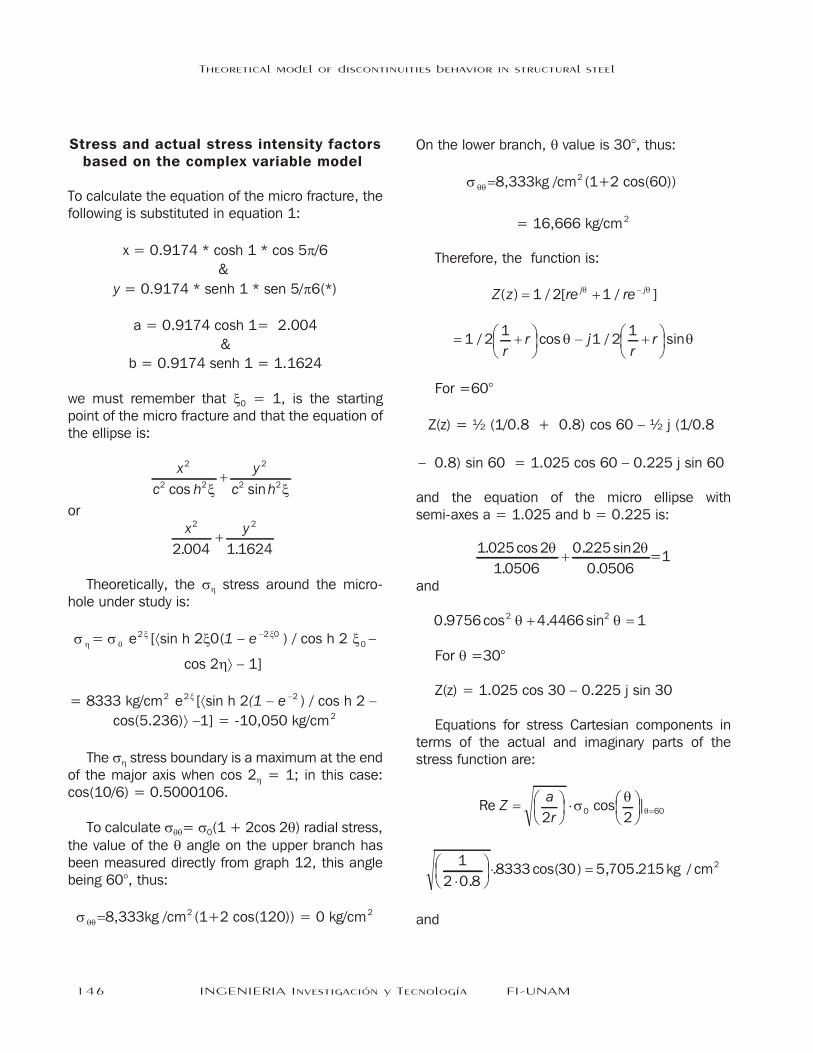
Stress and actual stress inten sity factors based on the complex variable model

To calculate the equation of the micro fracture, thefollowing is substituted in equation 1:

x = 0.9174 * cosh 1 * cos 5p/6

&

y = 0.9174 * senh 1 * sen 5/p6(*)

a = 0.9174 cosh 1= 2.004

&

b = 0.9174 senh 1 = 1.1624

we must remember that x0 = 1, is the startingpoint of the micro fracture and that the equation ofthe ellipse is:

x

c h

y

c h

2

2 2

2

2 2cos sinx x+

orx y2 2

2 004 1 1624. .+

Theoretically, the sh stress around the micro-hole under study is:

s h = s 0 0 e2x2[ásin h 2x00(1 – e -2 0x

-20) / cos h 20 x0 –

cos 2hñ – 1]

= 8333 kg/cm2 e2x [ásin h 2(1 – e -2-2) / cos h 2 –

cos(5.236)ñ –1] = -10,050 kg/cm2

2

The sh stress boundary is a maximum at the end of the major axis when cos 2h = 1; in this case:cos(10/6) = 0.5000106.

To calculate sqq= s0(1 + 2cos 2q) radial stress, the value of the q angle on the upper branch hasbeen measured directly from graph 12, this anglebeing 60°, thus:

s qq =8,333kg /cm2 (1+2 cos(120)) = 0 kg/cm2

2

On the lower branch, q value is 30°, thus:

s qq =8,333kg /cm2 (1+2 cos(60))

= 16,666 kg/cm2

2

Therefore, the function is:

Z z re rej j( ) / [ / ]= + -1 2 1q q

= +æ

èç

ö

ø÷ - +æ

èç

ö

ø÷1 2

11 2

1/ cos / sin

rr j

rrq q

For =60°

Z(z) = ½ (1/0.8 + 0.8) cos 60 – ½ j (1/0.8

– 0.8) sin 60 = 1.025 cos 60 – 0.225 j sin 60

and the equation of the micro ellipse withsemi-axes a = 1.025 and b = 0.225 is:

1 025 2

1 0506

0 225 2

0 0506

. cos

.

. sin

.

q q+ =1

and

0 9756 4 4466 12 2. cos . sinq q+ =

For q =30°

Z(z) = 1.025 cos 30 – 0.225 j sin 30

Equations for stress Cartesian components interms of the actual and imaginary parts of thestress function are:

Re cos |Za

r= æ

èç

ö

ø÷ × æ

èç

ö

ø÷ =

2 20 60s

qq

1

2 0 88333 30 5 705 215 2

×

æ

èç

ö

ø÷× =

.. cos( ) , . kg / cm

and



Re cos |Za

r= æ

èç

ö

ø÷ × æ

èç

ö

ø÷ =

2 20 30s

qq

1

2 0 88333 15 6 363 34 2

×

æ

èç

ö

ø÷× =

.. cos( ) , . kg / cm

Along the line where q and y are both zero, weobtain:

s syy Za

rZ= = æ

èç

ö

ø÷ × =Re Re

20

1

2 0 8833 6 587 8 2

×

æ

èç

ö

ø÷ =

.. , . kg / cm

and its stress intensity factor is:

k aI = × × =p s0 1.7725 * 8,333 kg/cm2

= 14,769.86 kg/cm3/2

It must be noticed that, when observing figure14 and comparing it with figure 1, becomes evi-dent that a branch of the hyperbola has an anglesuch as that of the fracture under study, namely60º, and that radial stress value is zero. This hap-pens because when this hyperbola exists, the tip of the crack has disappeared and stress begins to bedistributed over a much greater surface, leading toa decrease of such value and bringing about achange of sign. It may also be observed that, thesmaller the hyperbola branch angle is, the greaterthe stress will be, which will tend to increase thecloser the stress gets to zero (which means that itgets closer to the tip of the fracture), confirmingthe singularity of the stress at the tip of the frac-ture.

Conclu sions

In micro fracture in figure 12 may be observed thatthe expansion of the crack at micrometric levelsbehaves in a fractal manner. Its equation is not

presented. The distribution of particles close to thetip of the Chevron-type notch is circular in the welldefined area of the plastic zone, which shows thatthe probe was subject to a high stress concen-tration. Applying the complex variable theory pro-vides a complete view of the complexity of thetheoretical problem involved. The w = (z) = ½(z +1/z) function transforms biunivocally both theinside and the outside of the unit circle on theoutside of the second case –1 £ u £ 1 of the actual axis. It may be observed that, when there is a micro fracture that has already taken a hyperbolic shapeand when the angle of some of its branches is 60ºto the horizontal, the stress value is zero. Com-paring the values of stress intensity factors taken at the laboratory and the theoretical results obtained,it may be ascertained that experimental values arethe result of the overall effect of the test on theprobe.

Acknowl edg ments

The authors want to thank research projects na-med Fractal and Fracture in Structural SamplesNo. 20040225 and No. 20050900. Financed bythe Instituto Politécnico Nacional. Mexico.

Refer ences

Arteaga Arcos, J. C and Casa nova del Angel, F.(2005). Pruebas de laboratorio para el análisisde micro discontinuidades en acero estructural.El Portulano de la Ciencia. Año V, vol I, núm.14, pp. 543-558. House Logiciels. Mexico.

American Society of Testing Mate rials (ASTM)(1993). Stan dard E 813-89: Stan dard TestMethod for Plane-Strain Frac tures Tough ness of Metallic Mate rials.

Dally, J W and Riley W F. (1991). “Exper i mentalStress Anal ysis” McGraw-Hill. USA.

N. E. Kochin, I. A. Kibel and N. V. Rosé. (1958).Hidrodinámica teórica. MIR.



Suggesting biog raphy

Anderson T.L. Frac ture mechanics. CRC Press.USA. 1995.

Amer ican Society of Testing Mate rials (ASTM)Stan dard E 399-90: Stan dard test method forplane-strain frac tures tough ness of metallic materials. 1993.

Casa nova del Angel F. La conceptualización ma-temática del pasado, el presente y el futuro dela arquitectura y su estructura fractal. El por-tulano de la ciencia, Año II, 1(4):127-148,Mayo de 2003. 2001.

Drexler E. Engines of creation. Anchor Books.USA. 1986.

Juárez-Luna G. y Ayala-Millán A.G. Aplicación de lamecánica de fractura a problemas de la geo-

tecnia. El portulano de la ciencia, Año III,1(9):303-318. Enero de 2003.

NASA. Fatigue crack growth computer programNasgro versión 3.0. Referente Manual. LyndonB. Johnson Space Center. USA. 2000.

Regimex. Catálogo de productos. México. 1994.Gran Enciclopedia Salvat. Vols. 12 y 19. Salvat

Editores S.A. Barce lona. 2000. Sears F.W. y Zemansky M.W. Física Universitaria.

Vol. 1. Adison Wesley Longman–Pearson Edu-cation. México. 1999.

Serway R.A. y Faughn J. S. Física. Prentice Hall–Pearson Educa tion. México. 2001.

Wilson J.D. Física. Segunda edición. Prentice Hall-Pearson Educa tion. México. Capítulos 22 al 24. 1996.



About the authors

Fran cisco Casa nova del Angel. Earned his doctorate degree in math e mat ical statis tics in 1981, and concluded his profes -

sional studies in math e mat ical statis tics in 1978, at the Université Pierre et Marie Curie, Paris VI. He earned his Master

of Science, majored in struc tures, in 1974, and his Bach elor of Science in Physics and Math e matics at the Higher School

of Engi neering and Archi tec ture, Instituto Politécnico Nacional (Mexico). He was math e matics consul tant for the United

Nations in 1981; Head of the Depart ment of Processes and Quan ti ta tive Methods of the Secretaría de Agricultura y

Recursos Hidráulicos up to 1985; Head of the Depart ment of Policy and Public Expen di tures and Trans fers of the

Secretaría de Agricultura y Recursos Hidráulicos up to 1986; Assis tant Director of Statis tical Processes of the Secretaría

de Turismo in 1987; and consul tant for Banco Mexicano SOMEX, S.N.C., from 1991 to 1992. He has been member of

the Sociedad Mexicana Unificada de Egresados en Física y Matemáticas of the Instituto Politécnico Nacional, the

Mexican Statis tical Asso ci a tion; the Inter na tional Statis tical Insti tute; and the Clas si fi ca tion Society of North America. He

has been granted several academic and scien tific prizes such as the SERFIN Envi ron mental National Price in 1990; the

Profes sional Excel lence Prize in 1998; the Medal for Merit in Teaching and the Medal Juan de Dios Bátiz in 2002, as well

as the Prize for Research, by the Instituto Politécnico Nacional, in the same year, among others. Fran cisco Casa nova has

been professor in the Instituto Politécnico Nacional since 1971 and General Director of Logiciels, S.A. de C.V., since

1985. He has published various books and arti cles in pres ti gious maga zines and is currently Publishing Manager of the

science maga zine “El Portulano de la Ciencia”.

Juan Carlos Arteaga-Arcos. Civil engi neer (IPN, 1995-2000), He post grad uate studies are M in S. with major in struc tures

(IPN, 2001-.2005). Diploma: Desarrollo de proyectos de Innovación tecnológica (IPN, 2006), Ph Dr (candi date) with

major in Advanced Tech nology (IPN, 2005-current). Someone congresses partic i pa tion are: “Comportamiento mecánico

de morteros de alta resistencia elaborados con cemento pórtland refinado” xv inter na tional mate rial research congress,

Cancún, Quintana Roo, México, august 20th to 24th, 2006. “Mechan ical behavior and char ac ter iza tion of mortars based

on port land cement processed by high-energy milling” 1st Inter na tional Confer ence on Advanced Construc tion Mate rials,

Monterrey, Nvo. León México, December 3rd to 6th, 2006. High energy ball milling as an alter na tive route to obtain

ultrafine portalnd cement. 14th Inter na tional Sympo sium on Metastable and Nano-Materials, Corfu, Greece, October

26th to 30th, 2007. High energy milling of port land-cement mortars precur sors for enhacing its mechan ical strength.

14th Inter na tional Sympo sium on Metastable and Nano-Materials and “caracterizacion de cemento ultrafino obtenido a

nivel laboratorio por molienda de alta energía” L Congreso Nacional de Física, Boca del Río, Veracruz, México.

Date post:	08-Apr-2020
Category:	Documents
Upload:	others
View:	3 times
Download:	0 times

Theoretical model of discontinuities behavior in structural steel … · 2019-09-30 · Theoretical...

Documents