October 25, 2010 1

THEORY OF DIELECTRIC ELASTOMERS

Zhigang Suo *

School of Engineering and Applied Sciences, Kavli Institute for Nanobio Science

and Technology, Harvard University, Cambridge, MA 02138

ABSTRACT In response to a stimulus, a soft material deforms, and the deformation provides

a function. We call such a material a soft active material (SAM). This review focuses on one

class of soft active materials: dielectric elastomers. Subject to a voltage, a membrane of a

dielectric elastomer reduces thickness and expands area, possibly straining over 100%. The

phenomenon is being developed as transducers for broad applications, including soft robots,

adaptive optics, Braille displays, and electric generators. This paper reviews the theory of

dielectric elastomers, coupling large deformation and electric potential. The theory is developed

within the framework of continuum mechanics and thermodynamics, and is motivated by

molecular pictures and empirical observations. The theory is used to describe nonlinear and

nonequilibrium behavior, such as electromechanical instability and viscoelasticity. It is hoped

that the theory will aid in the creation of materials and devices.

* Email: suo@seas.harvard.edu ** The work reviewed here was carried out over the last six years, supported by NSF (CMMI-0800161, Large deformation and instability in soft active materials), by MURI (W911NF-04-1-0170, Design and Processing of Electret Structures0; W911NF-09-1-0476, Innovative Design and Processing for Multi-Functional Adaptive Structural Materials), and by DARPA (W911NF-08-1-0143, Programmable Matter; W911NF-10-1-0113, Cephalopod-inspired Adaptive Photonic Systems). This paper is submitted to a special issue of Acta Mechanica Solida Sinica on the occasion of its 30th anniversary.

Report Documentation Page Form ApprovedOMB No. 0704-0188

Public reporting burden for the collection of information is estimated to average 1 hour per response, including the time for reviewing instructions, searching existing data sources, gathering andmaintaining the data needed, and completing and reviewing the collection of information. Send comments regarding this burden estimate or any other aspect of this collection of information,including suggestions for reducing this burden, to Washington Headquarters Services, Directorate for Information Operations and Reports, 1215 Jefferson Davis Highway, Suite 1204, ArlingtonVA 22202-4302. Respondents should be aware that notwithstanding any other provision of law, no person shall be subject to a penalty for failing to comply with a collection of information if itdoes not display a currently valid OMB control number.

1. REPORT DATE 25 OCT 2010 2. REPORT TYPE

3. DATES COVERED 00-00-2010 to 00-00-2010

4. TITLE AND SUBTITLE Theory of Dielectric Elastomers

5a. CONTRACT NUMBER

5b. GRANT NUMBER

5c. PROGRAM ELEMENT NUMBER

6. AUTHOR(S) 5d. PROJECT NUMBER

5e. TASK NUMBER

5f. WORK UNIT NUMBER

7. PERFORMING ORGANIZATION NAME(S) AND ADDRESS(ES) Harvard University,School of Engineering and Applied Sciences,KavliInstitute for Nanobio Science and Technology,Cambridge,MA,02138

8. PERFORMING ORGANIZATIONREPORT NUMBER

9. SPONSORING/MONITORING AGENCY NAME(S) AND ADDRESS(ES) 10. SPONSOR/MONITOR’S ACRONYM(S)

11. SPONSOR/MONITOR’S REPORT NUMBER(S)

12. DISTRIBUTION/AVAILABILITY STATEMENT Approved for public release; distribution unlimited

13. SUPPLEMENTARY NOTES

14. ABSTRACT In response to a stimulus, a soft material deforms, and the deformation provides a function. We call such amaterial a soft active material (SAM). This review focuses on one class of soft active materials: dielectricelastomers. Subject to a voltage, a membrane of a dielectric elastomer reduces thickness and expands area,possibly straining over 100%. The phenomenon is being developed as transducers for broad applications,including soft robots, adaptive optics, Braille displays, and electric generators. This paper reviews thetheory of dielectric elastomers, coupling large deformation and electric potential. The theory is developedwithin the framework of continuum mechanics and thermodynamics, and is motivated by molecularpictures and empirical observations. The theory is used to describe nonlinear and nonequilibriumbehavior, such as electromechanical instability and viscoelasticity. It is hoped that the theory will aid in thecreation of materials and devices.

15. SUBJECT TERMS

16. SECURITY CLASSIFICATION OF: 17. LIMITATION OF ABSTRACT Same as

Report (SAR)

18. NUMBEROF PAGES

55

19a. NAME OFRESPONSIBLE PERSON

a. REPORT unclassified

b. ABSTRACT unclassified

c. THIS PAGE unclassified

Standard Form 298 (Rev. 8-98) Prescribed by ANSI Std Z39-18

October 25, 2010 2

I. INTRODUCTION

1.1. Soft Active Materials for Soft Machines

The convergence of parts of biology and engineering has created exciting opportunities

of discovery, invention and commercialization. The overarching themes include using

engineering methods to advance biology, combining biology and engineering to invent medical

procedures, and mimicking biology to create engineering devices.

Machines in engineering use mostly hard materials, while machines in nature are often

soft. What does softness impart to the life of animals and plants? A conspicuous feature of life

is to receive and process information from the environment, and then move. The movements

are responsible for diverse functions, far beyond the function of going from place to place. For

example, an octopus can change its color at an astonishing speed, for camouflage and signaling.

This rapid change in color is mediated by thousands of pigment-containing sacs. Attach to the

periphery of each sac are dozens of radial muscles. By contracting or relaxing the muscles, the

sac increases or decreases in area in less than a second. An expanded sac may be up to about 1

mm in diameter, showing the color. A retracted sac may be down to about 0.1 mm in diameter,

barely visible to the naked eye [1].

As another example, in response to a change in the concentration of salt, a plant can

change the rate of water flowing through the xylem. This regulation of flow is thought to be

mediated by pectins, polysaccharides that are used to make jellies and jams. Pectins are long

polymers, crosslinked into a network. The network can imbibe a large amount of water and

swell many times its own volume, resulting in a hydrogel. The amount of swelling changes in

response to a change in the concentration of slat. The change in the volume of the hydrogel

alters the size of the microchannels in the xylem, regulating the rate of flow[2].

The above examples are concerned with animals and plants. But many more examples

are everywhere around and inside us. Consider the accommodation of the eye, the beating of

the heart, the sound shaped by the vocal folds, and the sound in the ear. Abstracting these

October 25, 2010 3

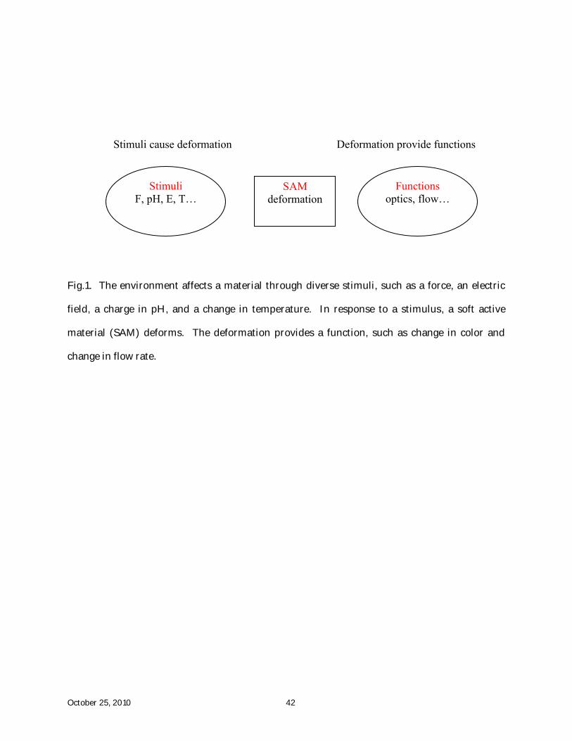
biological soft machines, we may say that a stimulus causes a material to deform, and the

deformation provides a function (Fig. 1). Connecting the stimulus and the function is the

material capable of large deformation in response to a stimulus. We call such a material a soft

active material (SAM).

An exciting field of engineering is emerging that uses soft active materials to create soft

machines. Soft active materials in engineering are indeed apt in mimicking the salient feature

of life: movements in response to stimuli. An electric field can cause an elastomer to stretch

several times its length. A change in pH can cause a hydrogel to swell many times its volume.

These soft active materials are being developed for diverse applications, including soft robots,

adaptive optics, self-regulating fluidics, programmable haptic surfaces, and oilfield

management[3-8].

Research in soft active materials has once again brought mechanics to the forefront of

human creativity. The familiar language finds new expressions, and deep thoughts are

stimulated by new experience. To participate in advancing the field of soft active materials and

soft machines effectively, mechanicians must retool our laboratories and our software, as well as

adapt our theories.

The biological phenomena, as well as the tantalizing engineering applications, have

motivated the development of theories of diverse soft active materials, including dielectric

elastomers[9-13], elastomeric gels[14-19], polyelectrolytes[20,21], pH-sensitive hydrogels[22-24], and

temperature sensitive hydrogels[25]. The theories attempt to answer commonly asked questions.

How do mechanics, chemistry, and electricity work together to generate large deformation?

What characteristics of the materials optimize their functions? How do molecular processes

affect macroscopic behavior? How efficiently can a material convert energy from one form to

another? The theories are being implemented in software, so that they can become broadly

useful in the creation of materials and devices.

October 25, 2010 4

1.2. Dielectric Elastomers

This review will focus on one particular class of soft active materials: dielectric

elastomers. All materials contain electrons and ions—charged particles that move in response

to an applied voltage. In a conductor, electrons or ions can move over a macroscopic distance.

By contrast, in a dielectric, the charged particles move relative to one another by short distances.

The two processes—deformation and polarization—are inherently coupled.

Fig.2 illustrates the principle of operation of a dielectric elastomer transducer. A

membrane of a dielectric elastomer is sandwiched between two compliant electrodes. The

electrodes have negligible electrical resistance and mechanical stiffness. A commonly used

material for such electrodes is carbon crease. The dielectric is subject to forces and voltage.

Charge flows through an external conducting wire from one electrode to the other. The charges

of the opposite signs on the two electrodes cause the membrane to deform. It was discovered

that an applied voltage may cause dielectric elastomers to strain over 100%[3]. Because of this

large strain, dielectric elastomers are often called artificial muscles. The discovery has inspired

intense development of dielectric elastomers as transducers for diverse applications[26-28].

This review focuses on the theory of dielectric elastomers. Section II describes the

thermodynamics of a transducer of two independent variations. Emphasis is placed on basic

ideas: states of the transducer, cyclic operation of the transducer, region of allowable states,

equations of state, stability of a state, and nonconvex free-energy function. These ideas are

described in both analytical and geometrical terms. Section III develops the theory of

homogeneous fields. After setting up a thermodynamic framework for electromechanical

coupling, we consider several specific material models: a vacuum as an elastic dielectric of

vanishing rigidity, incompressible materials, ideal dielectric elastomers, and electrostrictive

materials. Section IV applies nonequilibrium thermodynamics to dissipative processes, such as

viscoelasticity, dielectric relaxation, and electrical conduction. Section V discusses

electromechanical instability, both as a mode of failure and as a means to achieve giant voltage-

October 25, 2010 5

induced deformation. Section VI outlines the theory of inhomogeneous fields. A variational

statement is formulated as the basis for the finite element method. The associated partial

differential equations are summarized.

II. THERMODYANMICS OF A TRANSDUCER

2.1. States of a Transducer

Fig. 3 illustrates a transducer, consisting of a dielectric separating two electrodes. The

transducer is subject to a force P, represented by a weight. The two electrodes are connected

through a conducting wire to a voltage , represented by a battery. The weight moves by

distance l, and the battery pumps charge Q from one electrode to the other.

The transducer is capable of two independent variations. Consequently, states of the

transducer can be represented geometrically on a plane. The two coordinates of the plane may

be chosen from variables such as P, , l and Q. A point in the plane represents a state of the

transducer. For example, Fig. 4 shows the force P and the displacement l as the coordinates of

the plane. Plotted on the plane are the force-displacement curves of the transducer. Each force-

displacement curve is measured under the condition that the two electrodes are subject to a

constant voltage during deformation.

If the voltage between the electrodes can be varied, the force and the displacement may

be changed independently. When the transducer is subject to a constant weight, but the voltage

is changed from 0 to 1 , the transducer changes from state A to state B, lifting the weight.

When the displacement l is held constant, a change in the voltage causes the transducer to

change from state A to state C, with accompanying change in the force.

We could have also plotted on the Pl, plane curves of constant values of charge. Each

curve of a constant charge is the force-displacement curve of the transducer measured under the

open-circuit condition, when the two electrodes maintain a fixed amount of charge.

October 25, 2010 6

Following Gibbs’s graphical method for a thermodynamic system of fluids[29], we may

choose any two of the four variables P, , l and Q as coordinates. Each choice represents the

transducer on a different plane. All these planes represent the same states of the transducer,

because the transducer is capable only two independent variations. Nonetheless, different

planes emphasize different attributes of the states. For example, the ,P plane may be used

to indicate loading conditions, while the Ql, plane may be used to indicate kinematic

conditions. The ,l plane is often used to report the voltage-induced deformation, while the

QP, plane may be used to report force-induced charge.

2.2. Cyclic Operations of a Transducer

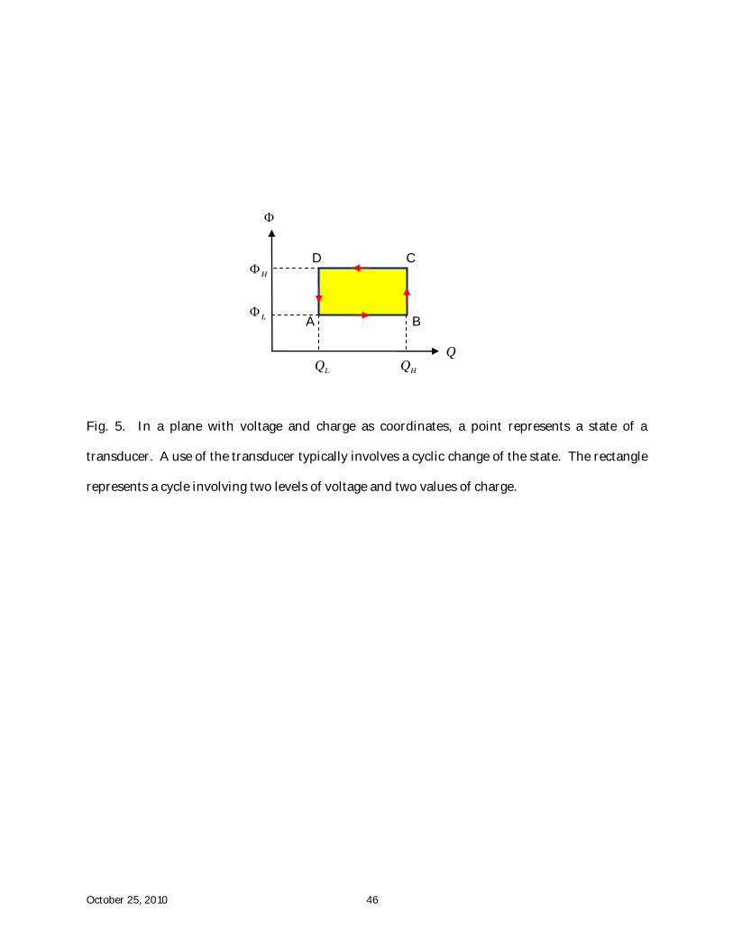
Most applications involve cyclic changes of the state of the transducer. A particular cycle

of states is illustrated in Fig. 5, on the ,Q plane. The voltage and the charge of the

transducer can be changed independently. In changing from state A to state B, the transducer is

connected to a battery of a low voltage, L ; a change in the applied force reduces the spacing

between the two electrodes, causing the charge on the electrodes to increase. In changing from

state B to state C, the transducer is under an open-circuit condition and the electrodes maintain

the constant charge HQ ; a change in the applied force increases the spacing between the two

electrodes, raising the voltage to H . In changing from state C to state D, the transducer is

connected to a battery of the high voltage H ; a change in the applied force increases the

spacing between the two electrodes, causing the charge on the two electrodes to decrease. In

changing from state B to state C, the transducer is under an open-circuit condition and the

electrodes maintain the constant charge LQ ; a change in the applied force decreases the spacing

between the two electrodes, lowering the voltage to L .

The cycle receives mechanical work, and pumps charge from a low voltage to a high

October 25, 2010 7

voltage. Such a cycle describes a generator, harvesting electric energy by receiving mechanical

work from the environment, such as the work done by an animal or human during walking, and

the work done by ocean waves.

Indeed, a closed curve of any shape on the ,Q plane represents a cyclic operation of

the transducer. The amount of energy converted per cycle is given by the area of the cycle on

the ,Q plane. When the states cycle counterclockwise on the ,Q plane, the transducer is

a generator, converting mechanical energy to electrical energy. When the states cycle clockwise

on the ,Q plane, the transducer is an actuator, converting electrical energy to mechanical

energy. The Pl, plane can also be used to evaluate energy of conversion per cycle.

2.3. Modes of Failure and Region of Allowable States

A transducer may fail in multiple modes, such as mechanical rupture, electrical

breakdown, electromechanical instability, and loss of tension[30-32]. The critical condition for

each mode of failure can be represented on the ,Q plane by a curve. Curves of all modes of

failure bound in the plane a region, which we call the region of allowable states of the transducer.

Such graphic methods have been used to optimize actuators[33,34] and calculate the maximal

energy of conversion for generators[35-37]. Fig. 6 shows an example[35].

2.4. Equations of State

On dropping a small distance l , the weight does work lP . On pumping a small

amount of charge Q , the battery does work Q . The force is work-conjugate to the

displacement, and the voltage is work-conjugate to the charge. We will analyze isothermal

processes, and remove temperature from explicit consideration. Denote the Helmholtz free

energy of the transducer by F. When the transducer equilibrates under the applied force and

the applied voltage, the change in the free energy of the transducer equals the sum of the work

October 25, 2010 8

done by the weight and the work done by the battery:

QlPF . (1)

This condition of equilibrium holds for arbitrary small variations l and Q . The displacement

and the charge are independent variables.

The two independent variables Ql, characterize the state of the transducer. The

Helmholtz free energy of the transducer is a function of the two independent variables:

QlFF , . (2)

Associated with small variations l and Q , the free energy varies by

QQ

QlFl

l

QlFF

,,. (3)

A comparison of (1) and (3) gives

0,,

Q

Q

QlFlP

l

QlF . (4)

When the transducer equilibrates with the weight and the battery, the condition of equilibrium

(4) holds for independent and arbitrary variations l and Q . Consequently, in equilibrium,

the coefficients of the two variations in (4) both vanish, giving

l

QlFP

,, (5)

Q

QlF

,. (6)

Once the free-energy function QlF , is known, (5) and (6) express P and as functions of l

and Q. That is, the two equations give the force and voltage needed to cause a certain

displacement and a certain charge. The two equations (5) and (6) constitute the equations of

state of the transducer.

Equation (5) can be used to determine the free-energy function from the force-

displacement curves of the transducer measured under the open-circuit conditions, when the

October 25, 2010 9

electrodes maintain constant charges. For each value of Q, the free energy is the area under the

force-displacement curve. Similarly, (6) can be used to determine the free-energy function from

the voltage-charge curves of the transducer. As mentioned before, Pl, and ,Q are

convenient planes to represent the states of the transducer when we wish to highlight work and

energy.

As an illustration, consider a parallel-plate capacitor—two plates of electrodes separated

by a thin layer of a vacuum (Fig. 7). The separation l between the two electrodes may vary, but

the area A of either electrode remains fixed. Recall the elementary fact that the amount of

charge on either electrode is linear in the voltage:

A

lQ

0 , (7)

where 0 the permittivity of the vacuum. Inserting (7) into (6) and integrating, we obtain the

free-energy function

A

lQQlF

0

2

2,

. (8)

Inserting (8) into (5), we obtain that

0

2

2 A

QP . (9)

Equations (7) and (9) constitute the equations of state of the parallel-plate capacitor. They are

readily interpreted. The applied voltage causes charge to flow from one electrode to the other,

so that one electrode is positively changed, and the other is negatively charged. Equation (7)

relates the charge to the applied voltage. The oppositely charged electrodes attract each other.

To maintain equilibrium, a force need be applied to the electrode. Equation (9) relates the

applied force to the charge.

Define the electric field by lE / and the stress by AP / . Rewrite (9) as

October 25, 2010 10

2

02

1E . (10)

This equation gives the stress needed to be applied to the electrodes to counteract the

electrostatic attraction. This stress is known as the Maxwell stress.

2.5. Stability of a State

The equations of state, (5) and (6), are in general nonlinear. If the transducer operates

in the neighborhood of a particular state Ql, , the equations of state can be linearized and

written in an incremental form:

QQl

QlFl

l

QlFP

,, 2

2

2

, (11)

QQ

QlFl

lQ

QlF

2

22 ,,

. (12)

We call 22 /, lQlF the mechanical tangent stiffness of the transducer, and 22 /, QQlF the

electrical tangent stiffness of the transducer. The two electromechanical coupling effects are

both characterized by the same cross derivative, lQQlFQlQlF /,/, 22 . Consequently,

the two electromechanical coupling effects reciprocate. The matrix

2

22

2

2

2

,,

,,

,

Q

QlF

Ql

QlF

Ql

QlF

l

QlF

QlH (13)

is known as the Hessian of the free-energy function QlF , .

As mentioned above, a state of the transducer can be represented by a point in the Ql, ,

as well as by a point in the ,P plane. For the same state of the transducer, the point in the

Ql, plane is mapped to the point in the ,P plane by the equations of state, (5) and (6). The

mapping may not always be invertible. That is, given a pair of the loads ,P , the equations of

October 25, 2010 11

state may not be invertible to determine a state Ql, . For example, (11) and (12) are not

invertible when the Hessian is a singular matrix, 0det H . This singularity may be understood

in terms of thermodynamics.

The transducer and the loading mechanisms (i.e., the weight and the battery) together

constitute a thermodynamic system. The free energy of the system is the sum of the free

energies of the individual parts—the transducer, the weight, and the battery. The free energy

(i.e., the potential energy) of a constant weight is Pl . The free energy of a battery of a constant

voltage is Q . Consequently, the free energy of the thermodynamic system combining the

transducer and the loading mechanisms is

QPlQlFQlG ,, . (14)

The system has two independent variables, l and Q.

Thermodynamics requires that the system should reach a stable state of equilibrium

when the free-energy function QlG , is a minimum against small changes in l and Q. When the

weight moves by l and the battery pumps charges Q , the free energy of the system varies by

22

222

2

2

2

,,

2

,

,,

QQ

QlFQl

Ql

QlFl

l

QlF

QQ

QlFlP

l

QlFG

(15)

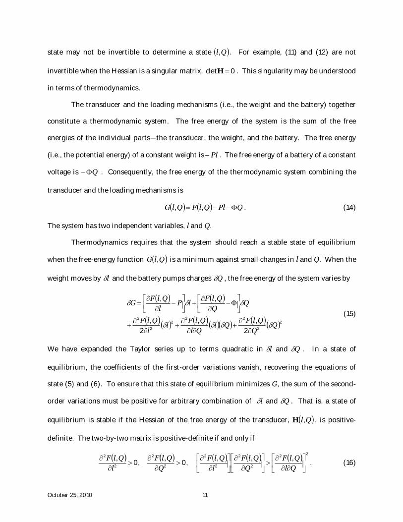
We have expanded the Taylor series up to terms quadratic in l and Q . In a state of

equilibrium, the coefficients of the first-order variations vanish, recovering the equations of

state (5) and (6). To ensure that this state of equilibrium minimizes G, the sum of the second-

order variations must be positive for arbitrary combination of l and Q . That is, a state of

equilibrium is stable if the Hessian of the free energy of the transducer, Ql,H , is positive-

definite. The two-by-two matrix is positive-definite if and only if

22

2

2

2

2

2

2

2

2 ,,,,0

,,0

,

Ql

QlF

Q

QlF

l

QlF

Q

QlF

l

QlF. (16)

October 25, 2010 12

When the Hessian of the free energy function is positive-definite, the function QlF , is convex

at this state Ql, .

As an illustration, consider the parallel-plate capacitor again. Given the free-energy

function (8), the second derivatives are

A

Q

Ql

QlF

A

l

Q

QlF

l

QlF

0

2

0

2

2

2

2 ,,

,,0

,

. (17)

Consequently, the Hessian is not positive-definite at any state of equilibrium. That is, the

parallel-plate capacitor subject to a constant force and a constant voltage cannot reach a stable

state of equilibrium. The conclusion is readily understood. The weight is independent of the

separation between the plates, but the electrostatic attractive force increases as the separation

decreases. Subject to a fixed weight, the two plates will be pulled apart if the voltage is small,

and will be pulled together if the voltage is small.

The capacitor can be stabilized by a modification of the loading mechanisms. For

example, we can replace the weight with a spring that restrains the relative movement of the

plates. Let K be the stiffness of the spring, and 0l be the separation between the electrodes when

the spring is unstretched, so that the force in the spring is llKP 0 . The free energy of the

system is the sum of the free energies of the capacitor, the spring and the battery:

QllKA

lQQlG

2

0

0

2

2

1

2,

. (18)

In a state of equilibrium, the first derivatives of QlG , vanish, giving the same equations of

state as (10) and (12). The state of equilibrium is stable if and only if the Hessian of QlG , is

positive-definite. The second derivatives of the function QlG , are

A

Q

Ql

QlG

A

l

Q

QlGK

l

QlG

0

2

0

2

2

2

2 ,,

,,

,

. (19)

A state of equilibrium Ql, is stable if and only if

October 25, 2010 13

2

00

A

Q

A

Kl

. (20)

Thus, the transducer is stable when the applied voltage is sufficiently small.

2.6. Nonconvex Free-Energy Surface

Following Gibbs[38], we may interpret above analytical statements geometrically.

Consider a three-dimensional space with Ql, as the horizontal plane, and F as the vertical axis.

In this space, the Helmholtz free energy QlF , is represented by a surface. A pair of the loads

,P is represented by an inclined plane passing through the origin of the space, with P as the

slope with respect to the l axis, and the slope of the tangent plane with respect to the Q axis.

By definition (14), the function QlG , is the vertical distance between the Helmholtz free

energy surface and the inclined plane. Thermodynamics dictates that this vertical distance

QlG , should minimize when the transducer equilibrates with the loads.

When the loads ,P are given, we may picture a plane simultaneously parallel to the

inclined plane and tangent to the free-energy surface QlF , . That is, the slope of the tangent

plane with respect to the l axis is P, and the slope of the tangent plane with respect to the Q axis

represents is . From the geometry, it is evident that the state Ql, of the tangent point

minimizes the vertical distance QlG , . Also evident from the geometry, QlG , is minimum

only if the free-energy surface QlF , in the neighborhood of the state Ql, is above the tangent

plane—that is, the surface QlF , is convex at the state Ql, .

When the loads ,P change gradually, so are the slopes of the inclined plane.

Consequently, as the loads ,P change gradually, the associated tangent plane rolls along the

free-energy surface. If the free-energy surface QlF , is globally convex, every tangent plane

touches the surface at only one point, and only one state Ql, is associated with a pair of given

October 25, 2010 14

loads ,P . By contrast, if part of the free-energy surface QlF , is concave, a tangent plane

may touch the surface at two points, and two states Ql, are associated with a pair of given

loads ,P .

It was discovered that the free energy functions for dielectric elastomers are typically

nonconvex[39]. Associated with a given set of loads, more than one states of equilibrium may

exist. The practical significance of nonconvex free-energy functions will be discussed later in

connection with electromechanical instability.

III. HOMOGENEOUS FIELD

We now develop a field theory of deformable dielectrics. The field theory assumes that a

material is a sum of many small pieces, and the field in each small piece is homogeneous. This

assumption enables us to define quantities per unit length, per unit area, and per unit volume.

This section focuses on the homogeneous field of a small piece, and Section VI considers

inhomogeneous field of a body by summing up small pieces.

This section begins by setting up a thermodynamic framework for electromechanical

coupling. We then consider several specific material models: a vacuum as an elastic dielectric of

vanishing rigidity, incompressible materials, ideal dielectric elastomers, and electrostrictive

materials.

3.1. Equations of State

With reference to Fig. 2, consider a block of an elastic dielectric, sandwiched between

two compliant electrodes. In the reference state, the dielectric is subject to no forces and

voltage, and is of dimensions 1L , 2L and 3L . In the current state, the dielectric is subject to

forces 1P , 2P and 3P , and the two electrodes are connected to a battery of voltage through a

conducting wire. In the current state, the dimensions of the dielectric become 1l , 2l and 3l , the

October 25, 2010 15

two electrodes accumulate electric charges Q , and the Helmholtz free energy of the

membrane is F .

When the dimensions of the dielectric change by 1l , 2l and 3l , the forces do work

332211 lPlPlP . When a small quantity of charge Q flows through the conducting wire, the

voltage does work Q . When the dielectric equilibrates with the forces and the voltage, the

increase in the free energy equals the work done:

QlPlPlPF 332211 . (21)

The condition of equilibrium (21) holds for arbitrary small variations of the four independent

variables, 1l , 2l , 3l and Q.

Define stretches by 111 Ll , 222 Ll and 333 Ll , nominal stresses by

3211 / LLPs , 3122 / LLPs and 2133 / LLPs , nominal electric field by 3/~

LE ,

nominal electric displacement by 21

~LLQD , and nominal density of the Helmholtz free

energy by 321 LLLFW . Also define true stresses by 3211 / llP , 3122 / llP and

2133 / llP , true electric field by 3/lE , and true electric displacement by 21llQD .

The condition of equilibrium (21) holds in any current state. However, it is convenient

to divide both sides of (21) by 321 LLL , the volume of the block in the reference state. We obtain

that

DEsssW~~

332211 . (22)

The condition of equilibrium holds for arbitrary small variations of the four independent

variables, 1 , 2 , 3 and D~

.

As a material model, the nominal density of the Helmholtz free energy is prescribed as a

function of the four independent variables:

DWW~

,,, 321 . (23)

October 25, 2010 16

Inserting (23) into (22), we obtain that

0~~

~33

3

22

2

11

1

DE

D

Ws

Ws

Ws

W

. (24)

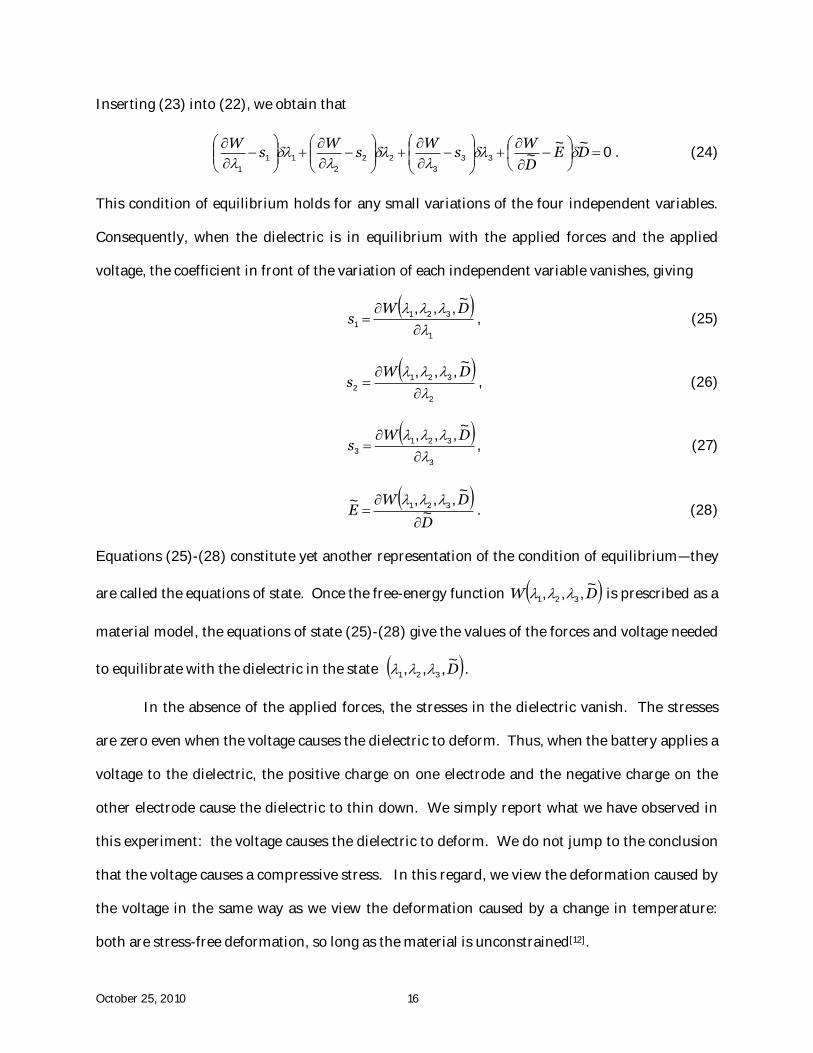
This condition of equilibrium holds for any small variations of the four independent variables.

Consequently, when the dielectric is in equilibrium with the applied forces and the applied

voltage, the coefficient in front of the variation of each independent variable vanishes, giving

1

321

1

~,,,

DWs , (25)

2

321

2

~,,,

DWs , (26)

3

321

3

~,,,

DWs , (27)

D

DWE ~

~,,,~ 321

. (28)

Equations (25)-(28) constitute yet another representation of the condition of equilibrium—they

are called the equations of state. Once the free-energy function DW~

,,, 321 is prescribed as a

material model, the equations of state (25)-(28) give the values of the forces and voltage needed

to equilibrate with the dielectric in the state D~

,,, 321 .

In the absence of the applied forces, the stresses in the dielectric vanish. The stresses

are zero even when the voltage causes the dielectric to deform. Thus, when the battery applies a

voltage to the dielectric, the positive charge on one electrode and the negative charge on the

other electrode cause the dielectric to thin down. We simply report what we have observed in

this experiment: the voltage causes the dielectric to deform. We do not jump to the conclusion

that the voltage causes a compressive stress. In this regard, we view the deformation caused by

the voltage in the same way as we view the deformation caused by a change in temperature:

both are stress-free deformation, so long as the material is unconstrained[12].

October 25, 2010 17

The work done by the battery, Q , can be written as

DELLLDLLELQ~~~~

321213 . (29)

That is, when a dielectric deforms, the nominal electric field and the nominal electric

displacement are work-conjugate. By contrast, in terms of the true electric field and the true

electric displacement, the work done by the battery is

DElllllEDlDllElQ 321213213 . (30)

For a deformable dielectric, 021 ll , so that the true electric displacement is not work-

conjugate to the true electric field[12].

3.2. Vacuum

As an application of the equations of state (25)-(28), consider a block of a vacuum. We

think of the vacuum as an elastic dielectric with vanishing rigidity, undergoing a homogenous

deformation 1 , 2 , and 3 . Recall an elementary fact that 2/2

0E is the electrostatic energy of

block divided by the block in the current state. Consequently, the nominal density of free energy

is

321

2

02

1 EW . (31)

Recall that the true electric displacement relates to the true electric field as ED 0 , and

relates to the nominal electric displacement as 21/~

DD . We rewrite (31) in terms of the

stretches and the nominal electric displacement:

210

3

2

3212

~~

,,,

DDW . (32)

Inserting (32) into (25)-(28), we obtain that

2

2

10

3

2

12

~

Ds , (33)

October 25, 2010 18

1

2

20

3

2

22

~

Ds , (34)

210

2

32

~

Ds , (35)

210

3

~~

DE . (36)

Equations (33)-(36) can be expressed in terms of the true quantities as

2

012

1E , (37)

2

022

1E , (38)

2

032

1E , (39)

ED 0 . (40)

Equations (37)-(39) recover the stresses obtained by Maxwell[40]. They are valid when the

electric field is in direction 3.

The Maxwell stress is a tensor. We have already interpreted the component of the

Maxwell stress in the direction of the electric field. We now look at the two components of the

Maxwell stress transverse to the direction of the electric field. Fig.8 illustrates a classic

experiment of a capacitor, which is partly in the air and partly in a dielectric liquid. The applied

voltage causes the liquid to rise to a height h. The height results from the balance of the

Maxwell stress and the weight of the liquid. The Maxwell stress parallel to the electrodes in the

air is 2/2Eaa , where a is the permittivity of the air. The Maxwell stress parallel to the

electrodes in the liquid is 2/2Ell , where l is the permittivity of the liquid. The electric

field near the air/liquid interface is distorted, so that the above two formulas are correct only at

some distance away from the interface. Because al , the difference in the Maxwell stresses

in the two media will draw the liquid up against gravity. Examining the free-body diagram, and

October 25, 2010 19

balancing the electrostatic forces with the weight of the liquid, we obtain that

2/2Egh al , where g is the weight per unit volume of the liquid.

3.3. Incompressibility

When an elastomer undergoes large deformation, the change in the shape is typically

much larger than the change in the volume. Consequently, the elastomer is often taken to be

incompressible—that is, the volume of the material remains unchanged during deformation,

321321 LLLlll , so that

1321 . (41)

This assumption of incompressibility places a constraint among the three stretches. We regard

1 and 2 as independent variables, rewrite (41) as 213 /1 , and express 3 in terms of

1 and 2 :

2

21

2

2

2

1

13

. (42)

In terms of the variations of the independent variables, the condition of equilibrium (22)

becomes

DEs

ss

sW~~

2

1

2

2

3

21

2

2

1

3

1

. (43)

For an incompressible material, this condition of equilibrium holds for any small variations of

the three independent variables, 1 , 2 and D~

.

For an incompressible elastic dielectric, the density of the free energy is a function of the

three independent variables:

DWW~

,, 21 . (44)

Inserting (44) into (43), we obtain that

October 25, 2010 20

0~~

~2

1

2

2

3

2

2

1

2

2

1

3

1

1

DE

D

Wss

Wss

W

. (45)

Because 1 , 2 and D~

are independent variations, the condition of equilibrium (45) is

equivalent to three equations:

1

21

2

2

1

3

1

~,,

DWss , (46)

2

21

1

2

2

3

2

~,,

DWss , (47)

D

DWE ~

~,,~ 21

. (48)

The four equations, (41) and (46)-(48), constitute the equations of state for an incompressible

dielectric elastomer.

3.4. Ideal Dielectric Elastomers

An elastomer is a three-dimensional network of long and flexible polymers, held

together by crosslinks (Fig. 9). Each polymer chain consists of a large number of monomers.

Consequently, the crosslinks have negligible effect on the polarization of the monomers: the

elastomer can polarize nearly as freely as a polymer melt. The permittivity changes by only a

few percent when the area of a membrane of an elastomer is stretched 25 times [41]. As an

idealization, we may assume that the dielectric behavior of an elastomer is exactly the same as

that of a liquid polymer, so that the density of free-energy function takes the form [39]

2

212

1, EWW s , (49)

where E is the true electric field, the permittivity, and 21 ,sW the free energy associated

with the stretching of the elastomer. The material is also taken to be incompressible, 1321 .

We call this material model the model of ideal dielectric elastomers.

October 25, 2010 21

The true electric displacement relates to the true electric field by ED , and relates to

the nominal electric field as 21

~DD . Consequently, in terms the nominal electric

displacement, (49) becomes

2

21

2121

~

2

1,

~,,

DWDW s . (50)

Inspecting (49) and (50), we note that the electromechanical coupling in an ideal dielectric

elastomer is purely a geometric effect.

Inserting (50) into (46)-(48) and taking the partial differentiations, we express the

results in terms of the true quantities:

2

1

21131

,E

Ws

, (51)

2

2

21232

,E

Ws

. (52)

ED . (53)

The above expression shows that a through-thickness electric field adds a compressive stress of

magnitude 2E in the two in-plane directions. This set of equations of state has been used

almost exclusively in all analyses of dielectric elastomers. The equations are usually justified in

terms of the Maxwell stress[3]. Now we have interpreted these equations using the model of

ideal dielectric elastomers. That is, the Maxwell stress is valid when the dielectric behavior of

the material is liquid-like, unaffected by deformation.

Observe that, in (51) and (52), the magnitude of the voltage-induced stress is twice the

magnitude of the Maxwell stress. This apparent difference is readily understood (Fig.10).

Because the elastomer is taken to be incompressible, superposition of a state of hydrostatic

stress does not affect the state of deformation. Start from the state of triaxial stresses

2/,2/,2/ 222 EEE , as derived by Maxwell, a superposition of a state of hydrostatic

October 25, 2010 22

stress 2/,2/,2/ 222 EEE gives a state of uniaxial stress 2,0,0 E , and a

superposition of a state of hydrostatic stress 2/,2/,2/ 222 EEE gives a state of biaxial

stress 0,, 22 EE . For an incompressible material, the three states of stress illustrated in

Fig. 10 cause the same state of deformation.

The free energy due the stretching of the elastomer, 21 ,sW , may be selected from a

large menu of well-tested functions in the theory of rubber elasticity. For example, the neo-

Hookean model takes the form

32

2

3

2

2

2

1

sW , (54)

where is the small-strain shear modulus.

In an elastomer, each individual polymer chain has a finite contour length. When the

elastomer is subject no loads, the polymer chains are coiled, allowing a large number of

conformations. Subjected to loads, the polymer chains become less coiled. As the loads

increase, the end-to-end distance of each polymer chain approaches the finite contour length,

and the elastomer approaches a limiting stretch. On approaching the limiting stretch, the

elastomer stiffens steeply. This effect is absent in the neo-Hookean model, but is represented by

the Arruda and Boyce model[43] and the Gent model[44]. The latter takes the form

lim

2

3

2

2

2

1lim3

1log2 J

JWs

. (55)

where is the small-stress shear modulus, and limJ is a constant related to the limiting stretch.

The stretches are restricted as 1/30 lim

2

3

2

2

2

1 J . When 0/3 lim

2

3

2

2

2

1 J , the

Taylor expansion of (55) is (54). That is, the Gent model recovers the neo-Hookean model when

deformation is small compared to the limiting stretch. When 1/3 lim

2

3

2

2

2

1 J , the free

energy diverges, and the elastomer approaches the limiting stretch.

October 25, 2010 23

3.5. Electrostriction

The voltage may cause some dielectrics to become thinner, but other dielectrics to

become thicker (Fig. 11). For dielectrics that are nonpolar in the absence of electric field, the

voltage-induced deformation has been analyzed by invoking stresses of two origins:

electrostriction and the Maxwell stress. The electrostriction results from the effect of

deformation on permittivity.

As a simplest model of electrostriction, we expand the free-energy function W into the

Taylor series in powers of E up to the quadratic term. The expansion is written in the form of

(49), but now the permittivity is a function of the stretches:

21 , . (56)

The same procedure as the above now gives the following equations of state[45]:

1

21

2

12

21

1

21131

,

2,

,

EE

Ws , (57)

2

21

2

22

21

2

21232

,

2,

,

EE

Ws , (58)

ED 21 , . (59)

The variation of the permittivity with stretches has been observed experimentally[46].

Further measurements are needed to ascertain the practical significance of electrostriction in

dielectric elastomers.

IV. NONEQUILIBRIUM THERMODYNAMIOCS OF DYELECTRIC ELASTOMERS

An elastomer responds to forces and voltage by time-dependent, dissipative processes[47-

49]. Viscoelastic relaxation may result from slippage between long polymers and rotation of

joints between monomers. Dielectric relaxation may result from distortion of electron clouds

and rotation of polar groups. Conductive relaxation may result from migration of electrons and

ions through the elastomer. This section describes an approach to construct models of

October 25, 2010 24

dissipative dielectric elastomers, guided by nonequilibrium thermodynamics[50].

Thermodynamics requires that the increase in the free energy should not exceed the

total work done, namely,

QlPlPlPF 332211 . (60)

For the inequality to be meaningful, the small changes are time-directed: f means the change

of the quantity f from one time to a slightly later time.

Divide both sides of (60) by the volume of the membrane, 321 LLL , and the

thermodynamic inequality becomes

DEsssW~~

332211 . (61)

As a model of the dielectric elastomer, the free-energy density is prescribed as a function:

,...,,~

,,, 21321 DWW . (62)

We characterize the state of a dielectric by 1 , 2 , 3 and D~

, along with additional parameters

,..., 21 . Inspecting (61), we note that 1 , 2 , 3 and D~

are the kinematic parameters through

which the external loads do work. By contrast, the additional parameters ,..., 21 are not

associated with the external loads in this way. These additional parameters describe the degrees

of freedom associated with dissipative processes, and are known as internal variables.

Inserting (62) into (61), we rewrite the thermodynamic inequality as

0~~

~33

3

22

2

11

1

i

i

i

WDE

D

Ws

Ws

Ws

W

. (63)

As time goes forward, this thermodynamic inequality holds for any change in the independent

variables ,...,,~

,,, 21321 D . We next specify a model consistent with this inequality.

We assume that the system is in mechanical and electrostatic equilibrium, so that in (63)

the factors in front of 1 , 2 and D~

vanish:

October 25, 2010 25

1

21321

1

, . . .,,~

,,,

DWs , (64)

2

21321

2

, . . .,,~

,,,

DWs , (65)

3

21321

3

, . . .,,~

,,,

DWs , (66)

D

DWE ~

,...,,~

,,,~ 21321

. (67)

Equations (64)-(67) constitute the thermodynamic equations of state of the dielectric elastomer.

Once the elastomer is assumed to be in mechanical and electrostatic equilibrium, the

inequality (63) becomes

0,...,,

~,,, 21321

i

i

i

DW

. (68)

This thermodynamic inequality may be satisfied by prescribing a suitable relation between

,..., 21 and ,.../,/ 21 WW . For example, one may adopt a kinetic model of the type

j j

iji

DWM

dt

d

, . . .,,~

,,, 21321 . (69)

Here ijM is a positive-definite matrix, which may depend on the independent variables

,...,,~

,,, 21321 D .

To represent a dissipative dielectric elastomer using the above approach, we need to

specify a set of internal variables ,..., 21 , and then specify the functions

,...,,~

,,, 21321 DW and ,...,,~

,,, 21321 DMij . There is considerable flexibility in

choosing kinetic models to fulfill the thermodynamic inequality (68).

Viscoelastic relaxation is commonly pictured with an array of springs and dashpots,

known as the rheological models; see a recent example[51]. Similarly, dielectric relaxation is

October 25, 2010 26

commonly pictured with models consisting of resistors and capacitors. By contrast, electrical

conduction involves the transport of charged species over a long distance. Coupled large

deformation and transport of charged species are significant in polyelectrolytes[21], and will not

be discussed here.

V. ELECTROMECHANICAL INSTABILITY

While all dielectrics deform under voltage, the amount of deformation differs markedly

among different materials. Under voltage, piezoelectric ceramics attain strains of typically less

than 1%. Glassy and semi-crystalline polymers can attain less than 10% [52]. Strains about 30%

were observed in some elastomers[53]. In the last decade, strains over 100% have been achieved

in several ways, by pre-stretching an elastomer[3], by using an elastomer of interpenetrating

networks[54,55], by swelling an elastomer with a solvent[56], and by spraying charge on an

electrode-free elastomer [57].

These experimental advances have prompted a theoretical question: What is the

fundamental limit of deformation that can be induced by voltage? One can easily increase the

length of a rubber band several times by using a mechanical force. Why is it difficult to do so by

using a voltage? The difficulty has to do with two modes of failure associated with apply a

voltage: electrical breakdown and electromechanical instability. For a stiff dielectric such as a

ceramic or a glassy polymer, voltage-induced deformation is limited by electrical breakdown,

when the voltage mobilizes charged species in the dielectric to produce a path of electrical

conduction.

For a compliant dielectric such as an elastomer, the voltage-induced deformation is

often limited by electromechanical instability. It was Stark and Garton[58] who first reported

that the breakdown fields of polymers reduced when the polymers became soft at elevated

temperatures. The phenomenon is understood as follows. The electric voltage is applied

between the electrodes on the top and the bottom surfaces of a thin layer of a polymer. As the

October 25, 2010 27

electric field increases, the polymer thins down, so that the same voltage will induce an even

higher electric field. This positive feedback results in a mode of instability, known as

electromechanical instability or pull-in instability, which causes the polymer to reduce the

thickness drastically, often leading to electrical breakdown. Electromechanical instability has

been recognized as a failure mode of the insulators for power transmission cables.

Electromechanical instability is sensitive to the stress-stretch behavior of the

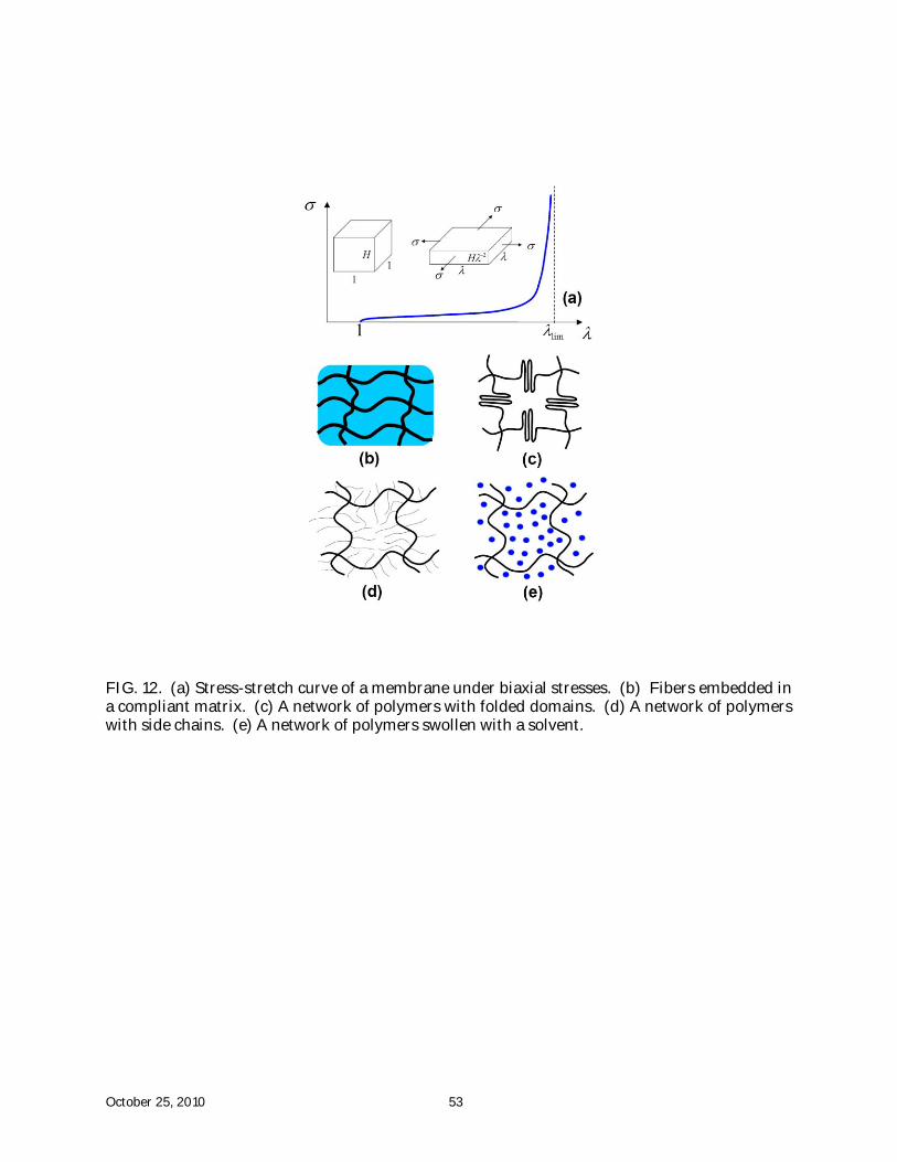
elastomer[39]. Fig. 12a sketches a dielectric membrane pulled by biaxial stresses . The length

of the membrane in any direction in the plane is stretched by a ratio . As will become clear, to

attain a large voltage-induced stretch, the dielectric should have a stress-stretch curve of

the following desirable features[59]: (a) The dielectric is compliant at small stretches, and (b) the

dielectric stiffens steeply at modest stretches. That is, the limiting stretch, lim , should not be

excessive. Also sketched are several designs of materials that exhibit the stress-stretch curve of

the desirable form. Many biological tissues, such as skins and vascular walls, deform readily,

but avert excessive deformation. Fig. 12b sketches a design of such a tissue, consisting of stiffer

fibers in a compliant matrix. At small stretches, the fibers are loose, and the tissue is compliant.

At large stretches, the fibers are taut, and the tissue stiffens steeply. As another example, Fig.

12c sketches a network of polymers with folded domains. The domains unfold when the

network is pulled, giving rise to substantial deformation. After all the domains unfold, the

network stiffens steeply.

Consider a synthetic elastomer, i.e., a network of polymer chains. When the individual

chains are short, the initial modulus of the elastomer is large and the limiting stretch lim is

small. When the individual chains are long, the initial modulus of the elastomer is small and the

limiting stretch lim is large. Consequently, it is difficult to achieve the stress-stretch curve of

the desirable form by adjusting the density of crosslinks alone. The stress-stretch curve,

however, can be shaped into the desirable form in several ways. For example, the widely used

October 25, 2010 28

dielectric elastomer, VHB, is a network of polymers with side chains (Fig. 12d). The side chains

fill the space around the networked chains. The motion of the networked chains is lubricated,

lowering the glass transition temperature. Also the density of the networked chains is reduced,

lowering the stiffness of the elastomer when the stretch is small. While the side chains do not

change the contour length of the networked chains, the side chains pull the networked chains

towards their full contour length even when the elastomer is not loaded. Once loaded, the

elastomer may stiffen sharply, averting electromechanical instability. Similar behavior is

expected for a network swollen with a solvent (Fig. 12e). The stress-stretch curve can also be

shaped into the desirable form by prestretch[3], or by using interpenetrating networks[54,55].

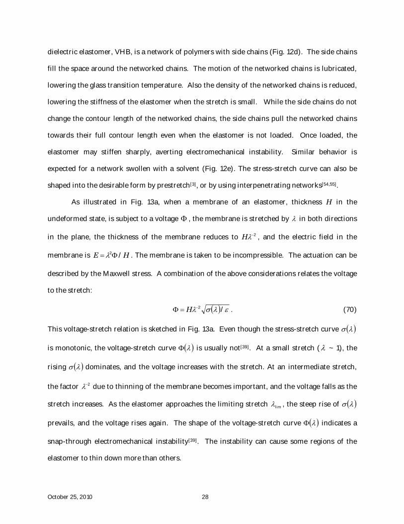
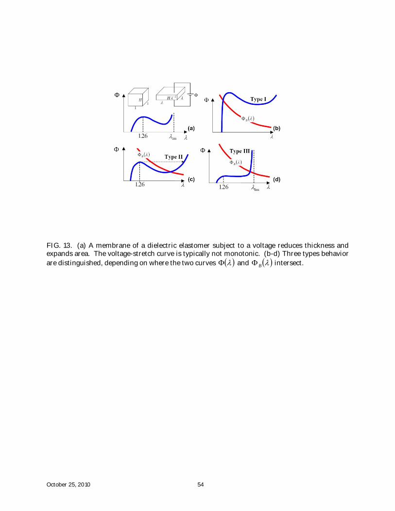
As illustrated in Fig. 13a, when a membrane of an elastomer, thickness H in the

undeformed state, is subject to a voltage , the membrane is stretched by in both directions

in the plane, the thickness of the membrane reduces to 2H , and the electric field in the

membrane is HE /2 . The membrane is taken to be incompressible. The actuation can be

described by the Maxwell stress. A combination of the above considerations relates the voltage

to the stretch:

/2 H . (70)

This voltage-stretch relation is sketched in Fig. 13a. Even though the stress-stretch curve

is monotonic, the voltage-stretch curve is usually not[39]. At a small stretch ( ~ 1), the

rising dominates, and the voltage increases with the stretch. At an intermediate stretch,

the factor 2 due to thinning of the membrane becomes important, and the voltage falls as the

stretch increases. As the elastomer approaches the limiting stretch lim , the steep rise of

prevails, and the voltage rises again. The shape of the voltage-stretch curve indicates a

snap-through electromechanical instability[39]. The instability can cause some regions of the

elastomer to thin down more than others.

October 25, 2010 29

The local maximum voltage represents a critical condition, which can be estimated as

follows. Under the equal-biaxial stresses, Hooke’s law takes the form 16 , where

is the shear modulus. Inserting this expression into (70), and maximizing the function ,

we find local maximum voltage /80.0 Hc and the critical 3 3.13/4 c . The critical

values vary somewhat with the stress-stretch relation. For example, for the neo-Hookean model,

42 , the maximum voltage is /6 9.0 Hc and the critical stretch is

2 6.12 3/1 c . This electromechanical instability has been analyzed systematically by using the

Hessian [60-64].

Before a voltage is applied, an elastomer may be prestretched to by a mechanical force,

and then fixed by rigid electrodes. Subsequently, when the voltage is applied, the elastomer will

not deform further. The measured voltage at failure is taken to be the electrical breakdown

voltage. Experiments indicate that the breakdown voltage is a monotonically decreasing

function of the prestretch, B [30,41].

According to where the curves and B intersect, we distinguish three types of

dielectric elastomers[59]. A type I dielectric suffers electrical breakdown prior to

electromechanical instability, and is capable of small deformation of actuation, Fig. 13b. A type

II dielectric reaches the peak of the curve, and thins down excessively, leading to electrical

breakdown, Fig. 13c. The dielectric is recorded to fail at the peak of , which can be much

below the breakdown voltage B . The deformation of actuation is limited by the stretch at

which the voltage reaches the peak. A type III dielectric eliminates or survives

electromechanical instability, reaches a stable state before the electrical breakdown, and attains

a large deformation of actuation, Fig. 13d.

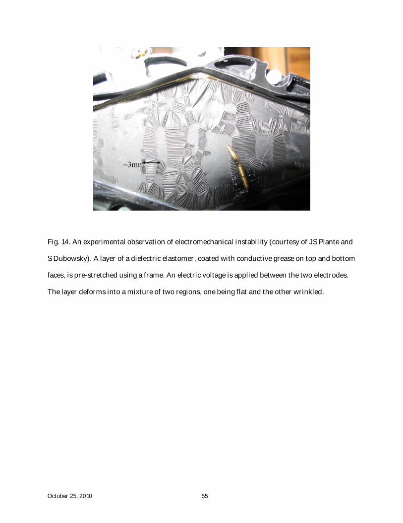
A new experimental manifestation of the electromechanical instability has been

reported recently[30]. Under certain conditions, an electric voltage can deform a layer of a

October 25, 2010 30

dielectric elastomer into a mixture of two regions, one being flat and the other wrinkled (Fig. 14).

In the experiment, the electrodes on the top and the bottom surfaces of the dielectric layer were

made of conducting grease, which applied a uniform electric potential to the elastomer without

constraining its deformation. This observation has been interpreted as the coexistence of two

states[39].

VI. INHOMOGENEOUS FIELDS

Studies of inhomogeneous fields of coupled large deformation and electric potential date

back to classic works of Toupin[66], Eringen[67] and Tiersten[68]. These works have been

reexamined recently for applications to dielectric elastomers[9-13]. Here we summarize basic

ideas, following the presentation of Ref. [12].

6.1. Condition of Thermodynamic Equilibrium

A body of an elastic dielectric is represented by a field of material particles. Each

material particle is named after the coordinate X of its place when the body is in a reference

state. In the current state, at time t, the particle X moves to a place with coordinate x. The

function

t,Xxx (71)

describes the history of the deformation of the body. Define the deformation gradient F as

K

iiK

X

txF

,X. (72)

The deformation gradient generalizes the notion of the stretches.

In the current state at time t, the electric potential at particle X is denoted as

t,X . (73)

The gradient of the electric potential defines the nominal electric field E~

, namely,

October 25, 2010 31

K

KX

tE

,~ X. (74)

The negative sign in (74) follows the convention that the electric field vector points in the

direction from a particle of a high voltage to a particle of a low voltage.

Motivated by (22), we write the variation of the nominal Helmholtz free energy, W , in

the form:

KKiKiK DEFsW~~

, (75)

where iKF is a small change in the deformation gradient, and KD~

is a small change in the

nominal electric field. Equation (75) defines the nominal stress s as a tensor work-conjugate to

the deformation gradient F, and the nominal electric displacement D~

as a vector work-

conjugate to the nominal electric field E~

.

Inspecting (72) and (74), we wish to use the deformation gradient and the nominal

electric field as the independent variables. Introducing a new quantity W by

KK DEWW~~ˆ . (76)

The quantity W may be called the electrical Gibbs free energy. A combination of (75) and (76)

gives

KKiKiK EDFsW~~ˆ . (77)

We may call the quantity KK ED~~ the complementary electrical work.

A material model is prescribed by a function EF~

,ˆˆ WW . When the body undergoes a

rigid body motion, the free energy is invariant. Consequently, the function depends on the

deformation gradient through the Green deformation tensor, iLiKKL FFC . Associated with

small changes iKF and KE~

, the electrical Gibbs free energy changes by

K

K

iK

iK

EE

WF

F

WW

~~

~,ˆ~

,ˆˆ

EFEF. (78)

October 25, 2010 32

On each material element of volume XdV , we prescribe mass dVX , force

dVt,XB and charge dVtq ,X . The effect of inertia may be represented by adding to the

force the inertial force, so that the net force on the element of volume is dVxtxB iii 22 / .

On each material element of interface XdA , we prescribe force dAt,XT and charge

dAt,X .

Let Xiix be a field of virtual displacement of the body—that is, every material

particle X moves independently. The virtual displacement Xi is unrelated to actual

displacement txi ,X . Associated with the field of virtual displacement, the forces do virtual

work dAxTdVxtxB iiiii 22 / . Similarly, let X be a field of virtual electric

potential of the body. Associated with the field of electric potential, the charges do virtual

complementary work dAdVq . The virtual deformation gradient is

KiiK XF /X , the virtual nominal electric field is KK XE /~

X , and the virtual

change in the electrical Gibbs free energy is dVW , where W is given by (78). When the

body is in thermodynamic equilibrium, the change in the electrical Gibbs free energy equals the

mechanical work minus the complementary electrical work:

dAdVqdAxTdVx

t

xBdVW iii

ii

2

2

ˆ . (79)

This condition of thermodynamic equilibrium has the similar physical content as (1) and (21),

and holds for arbitrary and independent variations x and .

Once the loads and the electrical Gibbs free-energy function EF~

,W are prescribed, the

variational statement (79), along with the definitions (72) and (74), is the basis for the finite

element method, determining the field of deformation t,Xx and the field of electric potential

t,X simultaneously. Several implementations of the finite element method have been

October 25, 2010 33

reported[65,69-71], but few practical examples are available, especially transducers approach

electromechanical instability. Significant effort is needed to develop the finite element method,

and to apply the method to analyze phenomena and devices.

6.2. Differential Equations

The variational statement of thermodynamic equilibrium also leads to partial differential

equations. These equations are listed in this subsection.

A comparison of (77) and (78) gives that

iK

iKF

Ws

EF~

,ˆ, (80)

K

KE

WD ~

~,ˆ~

EF. (81)

Once the electrical free-energy function EF~

,W is prescribed, (80) and (81) constitute the

equations of states.

Inserting (72), (74) and (77) into the condition of thermodynamic equilibrium (79), and

recalling that the condition holds for arbitrary and independent variations in x and , we

obtain that

2

2 ,,

,

t

txtB

X

ts ii

K

iK

XXX

X (82)

in the volume

iKiKiK TNss (83)

on an interface,

tq

X

tD

K

K ,,

~

XX

(84)

in the volume, and

tNDD KKK ,~~

X (85)

October 25, 2010 34

on the interfaces. Equations (82) and (83) reproduce the equations for momentum balance,

and (84) and (85) reproduce Gauss’s law of electrostatics.

Equations (71)-(74) and (80)-(85) are governing equations to determine the field of

deformation t,Xx and the field of electric potential t,X simultaneously, once the loads

and the free-energy function EF~

,W are prescribed. These partial differential equations have

been used to solve boundary-value problems involving coupled large deformation electric

potential[72-76]. Observe that the equations of mechanics, (71), (72), (82) and (83), decouple

from those of electrostatics, (73), (74), (84) and (85). The only coupling between mechanics

and electrostatics arises from the material model, (80) and (81).

6.3. True Quantities

The true stress ij relates to the nominal stress by

iK

jK

ij sF

Fdet . (86)

The true electric displacement iD relates to the nominal electric displacement as

KiK

i DF

D~

detF . (87)

The true electric field iE relates to the nominal electric field as

KiKi EHE~

, (88)

where iKH is the inverse of the deformation gradient, namely, KLiLiK FH and ijjKiK FH .

The true quantities are functions of x and t, and satisfy the familiar partial differential equations

in mechanics and electrostatics.

6.4. Ideal Dielectric Elastomers

Toupin[66] noted that, for an isotropic elastic dielectric, the free-energy density is a

October 25, 2010 35

function of six invariants of the deformation gradient tensor and the electric field vector.

Function of this complexity is unavailable for any real material. Several further considerations

may reduce the complexity of the free-energy function somewhat, but are still far from being

useful in practice[12].

We next describe ideal dielectric elastomers—a material model nearly exclusively used in

the literature. As discussed before in connection with Fig. 9, for an ideal dielectric elastomer,

the dielectric behavior is the same as that of a liquid—that is, the dielectric behavior is

unaffected by deformation[39]. As a simplest model of a dielectric liquid, assume that the true

electric displacement mD is linear in the true electric field mE :

mm ED (89)

The permittivity is taken to be independent of deformation.

Using (87) and (88), we express (89) in terms of the nominal fields:

Fdet~~

mLmNLN HHED . (90)

Inserting (90) into (81) and integrating, we obtain the nominal density of the electrical Gibbs

free energy:

FFEF det~~

2

~,ˆ

mLmNLNs HHEEWW

. (91)

Here FsW is the free energy associated with the strength of the elastomer, which may be

selected from a large menu in the theory of elasticity. While the elastomer is nearly

incompressible, in the finite element method, it is convenient to allow the material to be

compressible with a large bulk modulus.

Insert (91) into (80), and recall mathematical identities iNmKiKmN HHFH / and

FF det/det iKiK HF . We obtain that

FF

det2

1~~

iKmLmNmLmKiNLN

iK

siK HHHHHHEE

F

Ws . (92)

October 25, 2010 36

This equation of state expresses the nominal stress as a function of the deformation gradient

and the nominal electric field.

A combination of (86) and (92) gives

ijmmji

iK

sjK

ij EEEEF

WF

2

1

det

F

F. (93)

This equation expresses the true stress as a function of the deformation gradient and the true

electric field. The contribution due to the deformation gradient results of the stretching of the

elastomer, and is the same as that in the theory of elasticity. The contribution due to the electric

field is identical to that derived by Maxwell[40]. When 0ij , (93) balances elasticity and

electrostatics, and determines the voltage-induced deformation. As commented before, the

Maxwell stress correctly accounts for the voltage-induced deformation only when the dielectric

behavior is liquid-like, an idealization works well with elastomers, but not for any other solid

dielectrics.

Equations (89) and (93) constitute the equations of state, for an ideal dielectric

elastomer, in terms of the true quantities. The equations of state exhibit one-way coupling: the

deformation does not affect the dielectric behavior, but the electric field contributes to the

stress-stretch relation. As noted before, the partial differential equations of mechanics

decouples from those of electrostatics. One may solve electrostatic boundary-value problems in

terms of the true fields, and then add the Maxwell stress in solving the elastic field. Of course,

the deformation will change the shape of the boundaries of the body. This change must be

included in solving the electrostatic problems. The one-way coupling may not bring any

advantage after all.

The model of ideal dielectric elastomers can be generalized to account for nonlinear

dielectric behavior, by replacing (89) with a nonlinear relation between the electric field and

electric displacement[12]. Nonlinear dielectric behavior may be significant at high electric fields.

Furthermore, the model of ideal dielectric elastomers can be modified to include dissipative

October 25, 2010 37

processes, such as viscoelasticity, dielectric relaxation, and electrical conduction[21,50].

VII. CONCLUDING REMARKS

A large number of examples in biology demonstrate that deformation of soft materials

connect diverse stimuli to many functions essential to the life. An exciting field of engineering is

emerging that uses soft active materials to create soft machines. To participate in advancing the

field of soft active materials and soft machines effectively, mechanicians must retool our

laboratories and our software, as well as adapt our theories. While theories are being developed

for diverse soft active materials, this review focuses on one class of soft active materials:

dielectric elastomers. This focus allows us to review the theory in some depth, within the

framework of nonlinear continuum mechanics and nonequilibrium thermodynamics, while

motivating the theory by empirical observations, molecular pictures and applications. It is

hoped that the theory will be used to develop software, study intriguing phenomena of

electromechanical coupling, and aid the creation of soft active materials and soft machines.

October 25, 2010 38

References 1. Mathger, L.M., Denton, E.J., Marshall, N.J. and Hanlon. R.T., Mechanisms and

behavioral functions of structural coloration in cephalopods, J. R. Soc. Interface, 2008, 6: S149-S163.

2. Zwieniecki, M.A., Melcher, P.J. and Holbrook, N.M., Hydrogel control of xylem hydraulic resistance in plants, Science, 2001, 291: 1059-1062.

3. Pelrine, R., Kornbluh, R., Pei, Q.B. and Joseph, J., High-speed electrically actuated elastomers with strain greater than 100%, Science, 2000, 287: 836-839.

4. Tanaka, T., Gels, Sci. Am., 1981, Jan. 244: 124-138. 5. Beebe, D.J., Moore, J.S., Bauer, J.M.,, Yu, Q., Liu, R.H., Devadoss, C. and Jo, B.H.,

Functional hydrogel structures for autonomous flow control inside microfluidic channels, Nature, 2000, 404: 588-590.

6. Calvert, P., Hydrogels for soft machines, Adv. Mater., 2009, 21: 743-756. 7. Liu, F. and Urban, M.W., Recent advances and challenges in designing stimuli-

responsive polymers, Prog. Polymer Sci., 2010, 35: 3-23. 8. Cai, S.Q., Lou, Y.C., Ganguly, P., Robisson, A., Suo, Z.G., Force generated by a swelling

elastomer subject to constraint. J. Appl. Phys., 2010, 107: 103535. 9. Goulbourne, N.C., Mockensturm, E.M., Frecker, M., A nonlinear model for dielectric

elastomer membranes, J. Appl. Mech., 2005, 72: 899–906. 10. Dorfmann, A. and Ogden, R.W., Nonlinear electroelasticity, Acta Mechanica, 2005, 174:

167-183. 11. McMeeking, R. M. and Landis, C.M., Electrostatic forces and stored energy for

deformable dielectric materials. J. Appl. Mech., 2005, 72: 581-590. 12. Suo, Z.G., Zhao, X.H. and Greene, W.H., A nonlinear field theory of deformable

dielectrics ., J. Mech. Phys. Solids, 2008, 56: 467-286. 13. Trimarco, C., On the Lagrangian electrostatics of elastic solids., Acta Mech., 2009, 204:

193-201. 14. Sekimoto, K., Thermodynamics and hydrodynamics of chemical gels, J. Phys. II, 1991, 1,

19-36. 15. Dolbow, J., Fried, E., Jia, H.D., Chemically induced swelling of hydrogels. J. Mech. Phys.

Solids, 2004, 52: 51-84. 16. Baek, S. and Srinivasa, A.R., Diffusion of a fluid through an elastic solid undergoing

large deformation, Int. J. Non-linear Mech., 2004, 39: 201-218. 17. Hong. W., Zhao, X.H., Zhou, J.X. and Suo, Z.G., A theory of coupled diffusion and large

deformation in polymeric gels. J. Mech. Phys. Solids, 2008, 56: 1779-1793. 18. Doi, M., Gel dynamics, J. Phys. Soc. Japan, 2009, 78: 052001. 19. Chester, S.A. and Anand, L., A coupled theory of fluid permeation and large

deformations for elastomeric materials, J. Mech. Phys. Solids, 2010, 58: 1879-1906. 20. Nemat-Nasser, S. and Li, J.Y., Electromechanical response of ionic polymer-metal

composites, J. Appl. Phys., 2000, 87: 3321–3331 21. Hong, W., Zhao, X.H., Suo, Z.G., Large deformation and electrochemistry of

polyelectrolyte gels, J. Mech. Phys. Solids, 2010, 58:558-577. 22. Baek, S. and Srinivasa, A.R., Modeling of the pH-sensitive behavior of an ionic gel in the

presence of diffusion. Int. J. Non-linear Mech., 2004, 39: 1301-1318. 23. Li, H., Luo, R., Birgersson, E., Lam, K.Y., Modeling of multiphase smart hydrogels

responding to pH and electric voltage coupled stimuli, J. Appl. Phys., 2007, 101: 114905. 24. Marcombe, R., Cai, S.Q., Hong, W., Zhao, X.H., Lapusta, Y., and Suo, Z.G., A theory of

constrained swelling of a pH-sensitive hydrogel, Soft Matter, 2010, 6: 784-793. 25. Cai, S.Q. and Suo, Z.G., Mechanics and chemical thermodynamics of a temperature-

sensitive hydrogel. Manuscript in preparation.

October 25, 2010 39

26. Shankar, R., Ghosh, T.K. and Spontak, R.J., Dielectric elastomers as next-generation polymeric actuators, Soft Matter, 2007, 3: 1116-1129.

27. Carpi, F., Electromechanically active polymers, Editorial introducing a special issue dedicated to dielectric elastomers, Polymer International, 2010, 59:277-278.

28. Brochu, P. and Pei, Q. B., Advances in dielectric elastomers for actuators and artificial muscles, Macromolecular Rapid Communications, 2010, 31: 10-36.

29. Gibbs, J.W., Graphical methods in the thermodynamics of fluids, Transactions of the Connecticut Academy, 1973, 2:309-342. (Available online at Google Books)

30. Plante, J.S. and Dubowsky, S., Large-scale failure modes of dielectric elastomer actuators, Int. J. Solids Structures, 2006, 43: 7727-7751.

31. Wissler, M. and Mazza, E., Mechanical behavior of acrylic elastomer used in dielectric elastomer actuators, Sensors Actuators A, 2007, 134: 494-504.

32. Kollosche, M. and Kofod, G., Electrical failure in blends of chemically identical, soft thermoplastic elastomers with different elastic stiffness, Appl. Phys. Lett., 2010, 96: 071904.

33. Lochmatter, P., Kovacs, G., and Michel, S, Characterization of dielectric elastomer actuators based on a hyperelastic film model, Sensors and Actuators A, 2007, 135: 748-757 .

34. Moscardo, M., Zhao, X.H., Suo, Z.G. and Lapusta, Y., On designing dielectric elastomer actuators, J. Appl. Phys., 2008, 104: 093503.

35. Koh, S.J.A., Zhao, X.H. and Suo, Z.G., Maximal energy that can be converted by a dielectric elastomer generator. Appl. Phys. Lett., 2009, 94: 262902.

36. Koh, S.J.A., Keplinger, C., Li, T.F., Bauer, S. and Suo, Z.G., Dielectric elastomer generators: How much energy can be converted? Transactions on Mechatronics, in press.

37. Diaz-Calleja., R., Llovera-Segovia, P., Energy diagrams and stability restrictions for electroelastic generators, J. Polymer Sci. B, 2010, 48: 2023-2028.

38. Gibbs, J.W., A method of geometrical representation of the thermodynamic properties of substances by means of surfaces, Transactions of the Connecticut Academy, 1973, 2:382-404. (Available online at Google Books)

39. Zhao, X.H., Hong, W. and Suo, Z.G., Electromechanical coexistent states and hysteresis in dielectric elastomers, Phys. Rev. B , 2007, 76: 134113.

40. Maxwell, J.C., A Treatise on Electricity and Magnetism, Volume 1, Chapter V, Mechanical action between two electrical systems, Oxford University Press, 1873. (Available online at Google Books)

41. Kofod, G., Sommer-Larsen, P., Kornbluh, R. and Pelrine, R., Actuation response of polyacrylate dielectric elastomers, J. Intell. Mater. Syst. Struct., 2003, 14: 787-793.

42. Treloar, L.R.G., The Physics of Rubber Elasticity, Oxford University Press, 1975. 43. Arruda, E. M. and Boyce, M. C. J. Mech. Phys. Solids 41, 389-412 (1993). 44. Gent, A. N., Rubber Chem. Technol 69, 59-61 (1996). 45. Zhao X. and Suo, Z.G., Electrostriction in elastic dielectrics undergoing large

deformation, J. Appl. Phys., 2008, 104: 123530. 46. Wissler, M. and Mazza, E., Electromechanical coupling in dielectric elastomer actuators,

Sensors and Actuators A, 2007, 138: 384-393. 47. Lochmatter, P., Kovacs, G., Wissler, M., Characterization of dielectric elastomers based

on a visco-hyperelastic film model, Smart Mater. Structures, 2007, 135: 748-757. 48. Ha, S.M., Wissler, M., Pelrine, R., Stanford S., Kovas, G., Pei, Q., Characterization of

electroelastomers based on interpenetrating polymer networks, Proc. SPIE, 2007. 6524: 652408.

49. Plante, J.-S. and Dubowsky, S., On the performance mechanisms of dielectric elastomer actuators, Sensors Actuators A, 2007, 137: 96-109.

October 25, 2010 40

50. Zhao, X.H., Koh, S.J.A., Nonequilibrium thermodynamics of dielectric elastomers, submitted to Int. J. Appl. Mech.

51. Silberstein M.N. and Boyce, M.C., Constitutive modeling of the rate, temperature, and hydration dependent deformation response of Nafion to monotonic and cyclic loading, J. Power Sources, 2010, 195: 5692-5706.

52. Zhang, Q. M., Bharti, V. and Zhao, X., Giant electrostriction and relaxor ferroelectric behavior in electron-irradiated poly(vinylidene fluoride-trifluoroethylene) copolymer, Science, 1998, 280: 2101-2104.

53. Pelrine, R. E., Kornbluh, R. D. and Joseph, J. P., Electrostriction of polymer dielectrics with compliant electrodes as a means of actuation, Sensors and Actuators A, 1998, 64: 77-85.

54. Ha, S. M., Yuan, W., Pei, Q. B., Pelrine, R. and Stanford, S., Interpenetrating polymer networks for high-performance electroelastomer artificial muscles, Adv. Mater., 2006, 18: 887-891 (2006).

55. Suo, Z.G., Zhu, J., Dielectric elastomers of interpenetrating networks, 2009, Appl. Phys. Lett., 2009, 95: 232909.

56. Shankar, R., Ghosh, T. K. and Spontak, R. J., Electroactive nanostructured polymers as tunable actuators, Adv. Mater., 2007, 19: 2218-2223.

57. Keplinger, C., Kaltenbrunner, M., Arnold, N. and Bauer, S., Röntgen’s electrode-free elastomer actuators without electromechanical pull-in instability, Proc. Nat. Acad. Sci., 2010, 107: 4505-4510.

58. Stark, K.H. and Garton, C.G., Electric strength of irradiated polythene. Nature, 1955, 176:1225–1226.

59. Zhao, X.H. and Suo, Z.G., Theory of dielectric elastomers capable of giant deformation of actuation, Phys. Rev. Lett., 2010, 104: 178302.

60. Zhao X. H. and Suo, Z. G., Method to analyze electromechanical stability of dielectric elastomers, Appl. Phys. Lett., 2007, 91: 061921.

61. Norris, A.N., Comments on ―Method to analyze electromechanical stability of dielectric elastomers‖, Appl. Phys. Lett., 2008, 92: 026101.

62. Diaz-Calleja, R., Riande, E. and Sanchis, M.J., On electromechanical stability of dielectric elastomers, Appl. Phys. Lett., 2008, 93: 101902.

63. Leng, J.S., Liu, L.W., Liu, Y.J., Yu, K., Sun, S.H., Electromechanical stability of dielectric elastomers, Appl. Phys. Lett., 2009, 94: 211901.

64. Xu, B.-X., Mueller, R., Classen, M. and Gross, D., On electromechanical stability analysis of dielectric elastomer actuators, Appl. Phys. Lett., 2010, 97: 162908.

65. Zhou, J.X., Hong, W., Zhao, X.H. and Suo, Z.G., Propagation of instability in dielectric elastomers, Int. J. Solids Structures, 2008, 45: 3739-3750.

66. Toupin, R.A., The elastic dielectric. J. Rational Mech. Anal. 1956, 5: 849-914. 67. Eringen, A.C., On the foundations of electroelastostatics. Int. J. Engng. Sci. 1963, 1: 127-

153. 68. Tiersten, H.F., On the nonlinear equations of thermoelectroelasticity. Int. J. Engng Sci.

1971, 9: 587-604. 69. Vu, D. K., Steinmann, P. and Possart, G., Numerical modelling of non-linear

electroelasticity, Int. J. Numerical Methods Engng., 2007, 70, 685-704. 70. Zhao X. H. and Suo, Z. G., Method to analyze programmable deformation of dielectric

elastomer layers, Appl. Phys. Lett., 2008, 93: 251902. 71. O’Brien, B., McKay, T., Calius, E., Xie, S., I. Anderson, Finite element modelling of

dielectric elastomer minimum energy structures, Appl. Phys. A, 2009, 94, 507-514. 72. Mockensturm, E.M. and Goulbourne, N., Dynamic response of dielectric elastomers, Int.

J. Non-Linear Mech., 2006, 41: 388-395.

October 25, 2010 41

73. Zhu, J., Stoyanov, H., Kofod, G. and Suo. Z.G., Large deformation and electromechanical instability of a dielectric elastomer tube actuator. J. Appl. Phys., 2010, 108, 074113.

74. Zhu, J., Cai, S.Q., Suo, Z.G., Resonant behavior of a membrane of a dielectric elastomer. Int. J. Solids Structures, 2010, 47: 3254-3262.

75. Zhu, J., Cai, S.Q., Suo, Z.G., Nonlinear oscillation of a dielectric elastomer balloon, Polymer International, 2010, 59: 378-383 .

76. He, T.H., Zhao, X.H. and Suo, Z.G., Equilibrium and stability of dielectric elastomer membranes undergoing inhomogeneous deformation, J. Appl. Phys., 2009, 106, 083522.

October 25, 2010 42

Fig.1. The environment affects a material through diverse stimuli, such as a force, an electric

field, a charge in pH, and a change in temperature. In response to a stimulus, a soft active

material (SAM) deforms. The deformation provides a function, such as change in color and

change in flow rate.

SAM

deformation

Functions

optics, flow…

Stimuli

F, pH, E, T…

Stimuli cause deformation Deformation provide functions

October 25, 2010 43

Fig. 2. A dielectric elastomer in the reference state and in a current state.

1P1P

2P

2PCurrent state

2l

1l

3l

Q

Q

1L

2L

3L

Reference state

3P

3P

October 25, 2010 44

Fig.3. A transducer consists of a dielectric separating two electrodes. The transducer is subject

to a force, represented by a weight P. The two electrodes are connected through a conducting

wire to a battery of voltage . The weight moves by distance l, and the battery pumps charge Q

from one electrode to the other.

battery

Q

Q

l P weight

dielectri

electrod

electrode

October 25, 2010 45

Fig. 4. In a plane with force and displacement as coordinates, a point represents a state of a

transducer. A curve of a constant voltage is the force-displacement curve measured when the

transducer is subject to a constant voltage.

l

0

1P

A

C

B

October 25, 2010 46

Fig. 5. In a plane with voltage and charge as coordinates, a point represents a state of a

transducer. A use of the transducer typically involves a cyclic change of the state. The rectangle

represents a cycle involving two levels of voltage and two values of charge.

Q

LQ HQ

H

LA

C

B

D

October 25, 2010 47

FIG. 6. A state of a dielectric membrane is represented by a point in the charge-voltage plane.

The coordinates are given in dimensionless forms. Plotted are curves representing various

modes of failure: electrical breakdown (EB), electromechanical instability (EMI), loss of tension

( 0s ), and rupture by stretch ( R ). These curves bound the region of allowable states of

the transducer. A cycle involving two levels of voltage and two values of charge is represented

by dotted lines.

s=0

=R

EB

EMI

E=0

October 25, 2010 48

Fig. 7. A parallel-plate capacitor consists of two electrodes separated by a thin gap of a vacuum.

When a voltage is applied, the two electrodes attract each other. The electrostatic attraction is

balanced by applying a force.

October 25, 2010 49

Fig. 8. A parallel-plate capacitor is partly in the air and partly in a liquid. When a voltage is

applied, the liquid rises. As indicated by the free-body diagram on the right, the rise of the

liquid is due to the balance between the Maxwell stress and the weight of the liquid.

h

2

02

1E

gh

2

2

1E

October 25, 2010 50

Fig. 9. An elastomer is a three dimensional network of long and flexible polymer chains. Each

polymer chain consists of a large number of monomers.

October 25, 2010 51

Fig.10. A dielectric in three states of stresses.

2E 2E

uniaxial

stress

biaxial stresses

2

2

1E

triaxial stresses

October 25, 2010 52

(b) (c)

+ + + + + + + + +

- - - - - - - - - -

+ + + + + + + + +

- - - - - - - - - -

(a) (b) (c)

+ + + + + + + + +

- - - - - - - - - -

+ + + + + + + + +

- - - - - - - - - -

(a)

Fig. 11. Consider a dielectric that is nonpolar in the absence of applied voltage (a). Subject to a

voltage, some dielectrics become thinner (b), but other dielectrics become thicker (c).

October 25, 2010 53

FIG. 12. (a) Stress-stretch curve of a membrane under biaxial stresses. (b) Fibers embedded in a compliant matrix. (c) A network of polymers with folded domains. (d) A network of polymers with side chains. (e) A network of polymers swollen with a solvent.

October 25, 2010 54

FIG. 13. (a) A membrane of a dielectric elastomer subject to a voltage reduces thickness and expands area. The voltage-stretch curve is typically not monotonic. (b-d) Three types behavior

are distinguished, depending on where the two curves and B intersect.

October 25, 2010 55

Fig. 14. An experimental observation of electromechanical instability (courtesy of JS Plante and

S Dubowsky). A layer of a dielectric elastomer, coated with conductive grease on top and bottom

faces, is pre-stretched using a frame. An electric voltage is applied between the two electrodes.

The layer deforms into a mixture of two regions, one being flat and the other wrinkled.

~3mm