THERMAL-FLUID CHARACTERIZATION AND PERFORMANCE …

THERMAL-FLUID CHARACTERIZATION AND PERFORMANCE ENHANCEMENT

OF DIRECT ABSORPTION MOLTEN SALT SOLAR RECEIVERS

by

Mélanie Tétreault-Friend

B.Eng., Mechanical Engineering, McGill University (2012)

M.S., Nuclear Science and Engineering, Massachusetts Institute of Technology (2014)

SUBMITTED TO THE

DEPARTMENT OF NUCLEAR SCIENCE AND ENGINEERING

IN PARTIAL FULFILLMENT OF THE REQUIREMENTS FOR THE DEGREE OF

DOCTOR OF PHILOSOPHY IN NUCLEAR SCIENCE AND ENGINEERING

AT THE

MASSACHUSETTS INSTITUTE OF TECHNOLOGY

JUNE 2018

© 2018 Massachusetts Institute of Technology

All rights reserved.

Signature of Author: _________________________


Department of Nuclear Science and Engineering

May 25, 2018

Certified by: ___________________________

Alexander H. Slocum

Walter M. May and A. Hazel May Professor of Mechanical Engineering

Thesis Supervisor

Certified by: ___________________________

Emilio Baglietto

Norman C. Rasmussen Associate Professor of Nuclear Science and Engineering

Thesis Supervisor

Certified by: ___________________________

Gang Chen

Carl Richard Soderberg Professor of Power Engineering

Thesis Reader

Accepted by: ___________________________

Ju Li

Battelle Energy Alliance Professor of Nuclear Science and Engineering

and Professor of Materials Science and Engineering Chair, Department Committee on Graduate Students

2

3

THERMAL-FLUID CHARACTERIZATION AND PERFORMANCE ENHANCEMENT

OF DIRECT ABSORPTION MOLTEN SALT SOLAR RECEIVERS

by


Submitted to the Department of Nuclear Science and Engineering

on May 25, 2018 in Partial Fulfillment of the

Requirements for the Degree of Doctor of Philosophy in

Nuclear Science and Engineering

Abstract

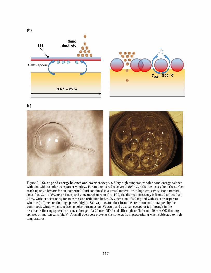
This thesis presents an in-depth thermal-fluid analysis of direct absorption molten salt solar

receivers. In this receiver concept, an open tank of semi-transparent liquid is directly irradiated

with concentrated sunlight, where it is absorbed volumetrically and produces internal heat

generation. The intensity distribution of the internal heating depends on the optical properties of

the absorber liquid and the dimensions of the receiver. This heating results in a combination of

thermal stratification and radiation-induced natural convection in the receiver, which govern the

general thermal-fluid behavior and performance of the system. Direct absorption requires molten

salts to be contained in open tanks directly exposed to the environment; consequently, the liquid

absorber experiences thermal losses to the environment which reduces absorption efficiency and

produces large temperature gradients immediately below the exposed liquid surface.

The thesis presents an apparatus that allows for the precise measurement of light attenuation in

high temperature, nearly transparent liquids. The apparatus is used to measure and characterize the

absorption properties of the 40 wt. % KNO3:60 wt. % NaNO3 binary nitrate and the

50 wt. % KCl:50 wt. % NaCl binary chloride molten salt mixtures. The analytical model of the

thermal stratification, radiation-induced convection, and radiative cooling effects highlights the

key parameters and conditions for optimizing the thermal-fluid performance of the receiver.

Computational fluid dynamics and heat transfer modeling of the CSPonD Demonstration prototype

of a direct absorption molten salt solar receiver provide further insight into its performance. The

findings from the analytical and computational analyses give motivation to create a new cover

design for open tanks of molten salts consisting of floating hollow fused silica spheres. The cover

concept is demonstrated experimentally and the analysis shows the cover’s ability to reduce

thermal losses by 50%.

Thesis Supervisor: Alexander H. Slocum

Walter M. May and A. Hazel May Professor of Mechanical Engineering

Thesis Supervisor: Emilio Baglietto

Norman C. Rasmussen Associate Professor of Nuclear Science and Engineering

4

5

In memory of Thomas J. McKrell,

Wherever you may be, I hope you found those mermaids…

R.I.P. 1969 - 2017

6

7

Acknowledgements

Dr. Thomas McKrell started me on my journey at MIT six years ago. He was an advisor, a mentor,

and a friend. He was a gentle force who shared his enthusiasm for science and his love for life

through his mentoring, and taught me to work hard and to appreciate the learning process. His

countless stories and anecdotes reminded me to also pause, reflect on life and science, and share

some good laughs. Tom left us during this journey, but his memory will always inspire me to be a

good scientist, and most importantly, a good person.

My PhD could also not have been possible without the help and support from countless faculty,

colleagues, and friends. First and foremost, I would like to thank my advisor, Prof. Alex Slocum,

for giving me the opportunity to collaborate on this massive project, for sharing his larger-than-

life enthusiasm, and for supporting my creativity. I would also like to thank my committee

members, Prof. Emilio Baglietto and Prof. Gang Chen, for their generous guidance and advice.

This work was supported by the Masdar Institute of Science and Technology, in collaboration with

Prof. Nicolas Calvet’s research group at the Masdar Institute Solar Platform. Special thanks to

Toni, Victor, Thomas, Radia, Benjamin, Peter, Dr. Charles Forsberg, and Miguel, for making

the CSPonD a reality. I would also like to thank Prof. Jacob Karni of the Weizmann Institute for

sharing his expertise in concentrated solar power and thermal energy storage. Thank you also to

Prof. Buongiorno for his continued interest in the CSPonD and for sharing experimental

equipement.

I had the privilege to collaborate with several research groups at MIT during this project. In

particular, NSE’s Green Lab has been my home for the past six years where Carolyn, Guanyu,

Andrew, Bren, Reza, and Matteo became my friends and family at MIT. I would like to thank

Prof. Gang Chen’s Nano group for graciously sharing their research space, and George, Lee, Hadi,

Tom, and Sveta, for sharing their expertise and guidance in solar thermal technology. NSE’s CFD

group provided invaluable computational support to a silly experimentalist. And a special thanks

to all PERGies for sharing your awesome lab environment and your inspiring creativity.

I also had the opportunity to mentor two talented undergraduate students, Shapagat Berdibek and

Luke Gray, who helped build and run extremely hot optical experiments. It was an honor to work

with you and I look forward to mentoring more students like you.

Finally, this work would not be possible without the behind-the-scenes support from family and

loved ones. In addition to my PhD, this project allowed me to find Miguel, the most kind, patient,

and understanding person I know. And of course thank you to my family, my brother, the infamous

trouble-makers Sherlock and Watson, and my courageous mother, for raising two engineers all on

her own.

“It may be the warriors who get the glory, but it’s the engineers who build societies.”

-B’Elanna Torres

8

9

Table of Contents

Abstract ....................................................................................................................................... 3

Acknowledgements ..................................................................................................................... 7

List of Figures ........................................................................................................................... 12

List of Tables ............................................................................................................................ 16

Nomenclature ............................................................................................................................ 17

1. Introduction ........................................................................................................................... 20

1.2. CSPonD Demonstration Project Test Facility ................................................................... 22

1.3. Participating media and natural convection in internally heated fluids ......................... 24

1.4. Molten Salts.................................................................................................................... 28

1.5. Thermal losses in open tanks of molten salt .................................................................. 31

1.6. Objectives ....................................................................................................................... 32

1.6.1. Scope of thesis ........................................................................................................ 33

2. Molten salt optical properties measurements ........................................................................ 35

2.1. Experimental Procedure ................................................................................................. 35

2.1.1. Apparatus description ............................................................................................. 35

2.1.2. Mixture preparation ................................................................................................ 39

2.1.3. Measurement procedure .......................................................................................... 41

2.2.3. Thermal performance evaluation ............................................................................ 41

2.3. Experimental Validation ................................................................................................ 45

2.4. Results ............................................................................................................................ 46

2.5. Discussion ...................................................................................................................... 51

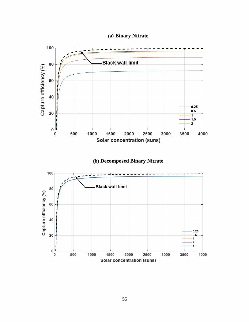
2.5.1. Volumetric absorption ............................................................................................ 51

2.5.2. Effective Emissivity ................................................................................................ 52

2.5.3. Capture Efficiency .................................................................................................. 53

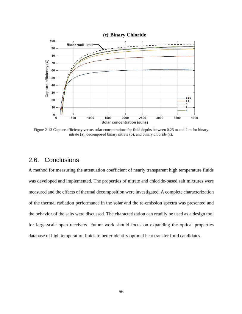
2.6. Conclusions .................................................................................................................... 56

10

3. Theoretical study of direct absorption receivers ................................................................... 57

3.1. Problem formulation ...................................................................................................... 58

3.2. Governing equations ...................................................................................................... 59

3.3. Model validation ............................................................................................................ 64

3.4. Direct absorption receiver optimization ......................................................................... 72

3.5. Conclusions .................................................................................................................... 77

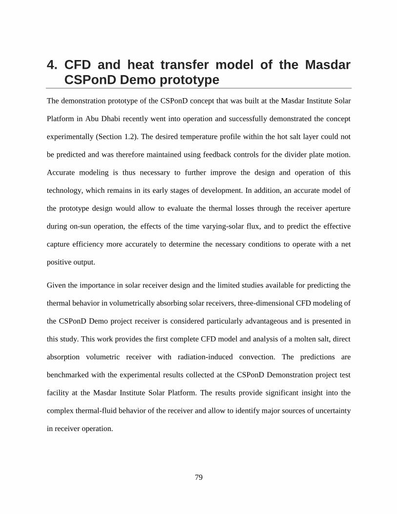
4. CFD and heat transfer model of the Masdar CSPonD Demo prototype ............................... 79

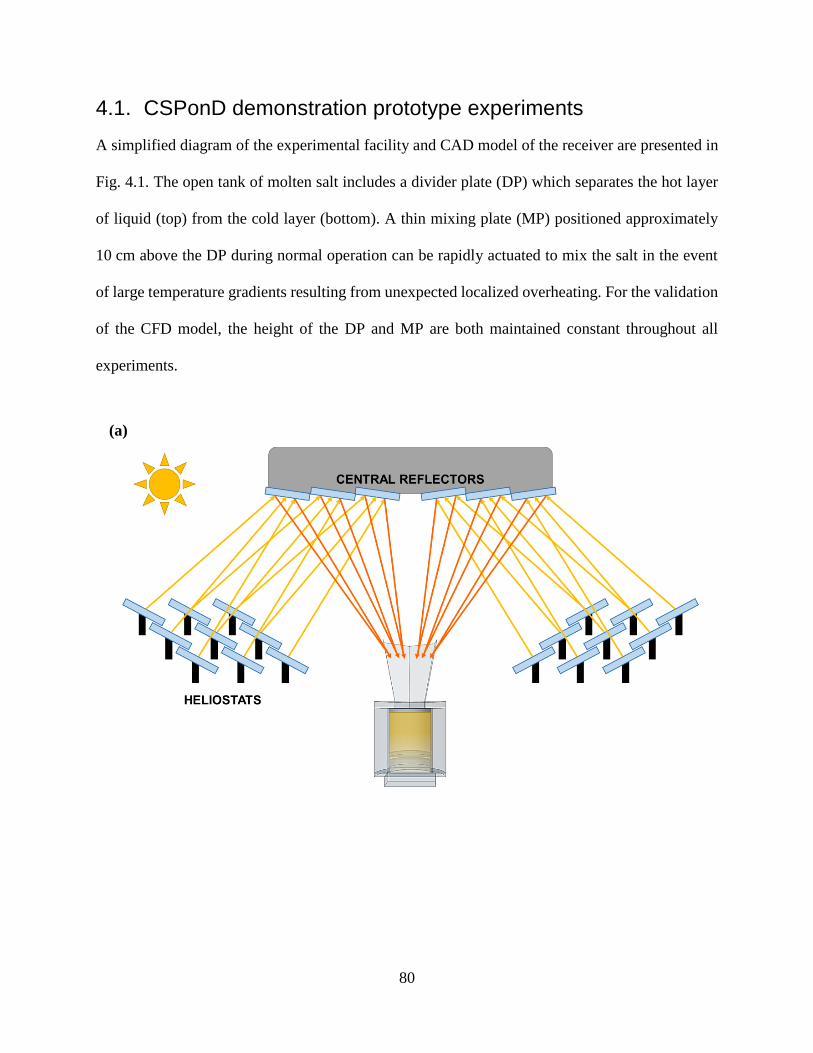
4.1. CSPonD demonstration prototype experiments ............................................................. 80

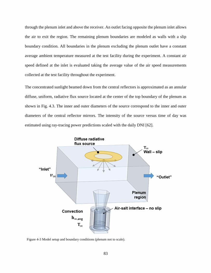
4.2. Model setup and boundary conditions ........................................................................... 82

4.3. Numerical procedure ...................................................................................................... 86

4.4. Dependence on the grid resolution ................................................................................. 91

4.5. Results for January 23, 2018 experiment ....................................................................... 95

4.5.1. Initial Conditions .................................................................................................... 95

4.5.2. Results: CFD calculated temperature and velocity distributions ............................ 99

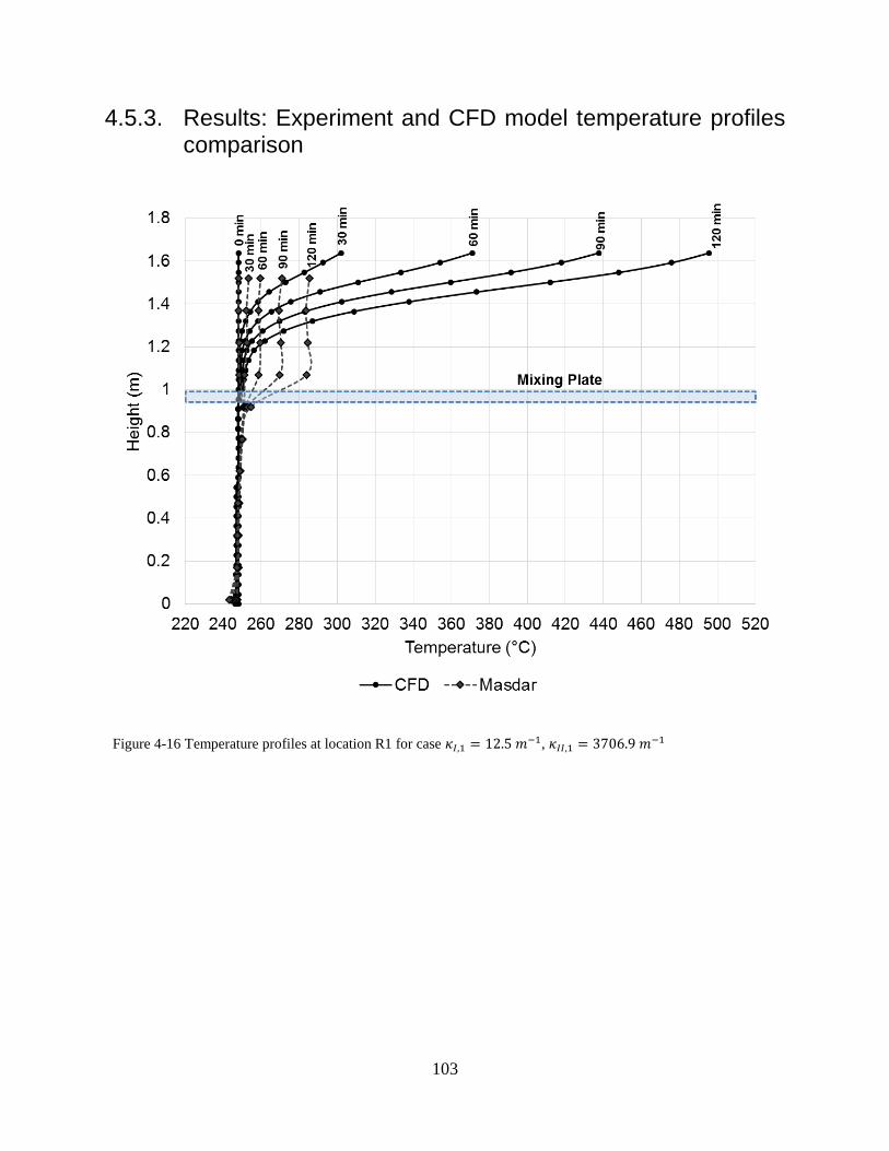
4.5.3. Results: Experiment and CFD model temperature profiles comparison .............. 103

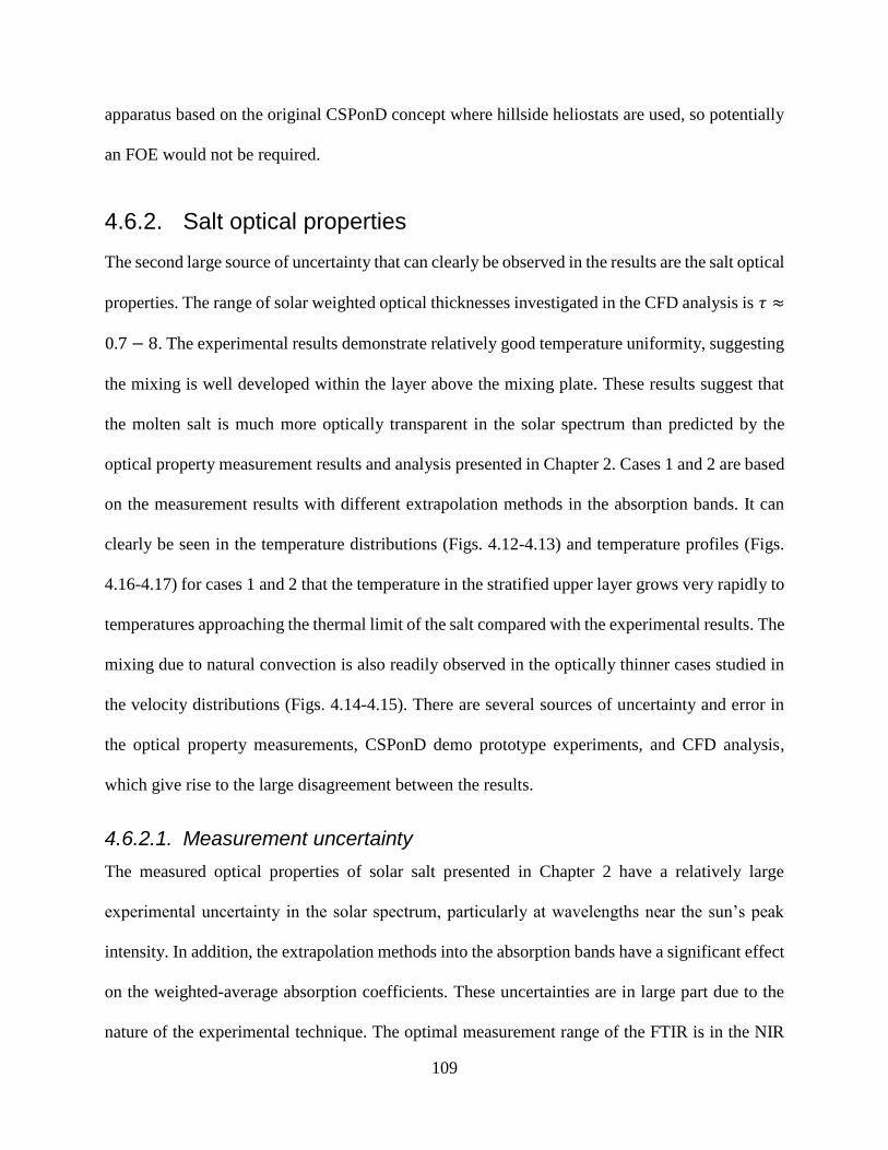
4.6. Discussion .................................................................................................................... 107

4.6.1. Solar source intensity ............................................................................................ 107

4.6.2. Salt optical properties ........................................................................................... 109

4.6.3. Demo prototype experimental uncertainty ............................................................ 111

4.7. Conclusions ...................................................................................................................... 112

5. Receiver cover design for enhanced thermal performance ................................................. 113

5.1. Very High Temperature Floating Modular Cover........................................................ 114

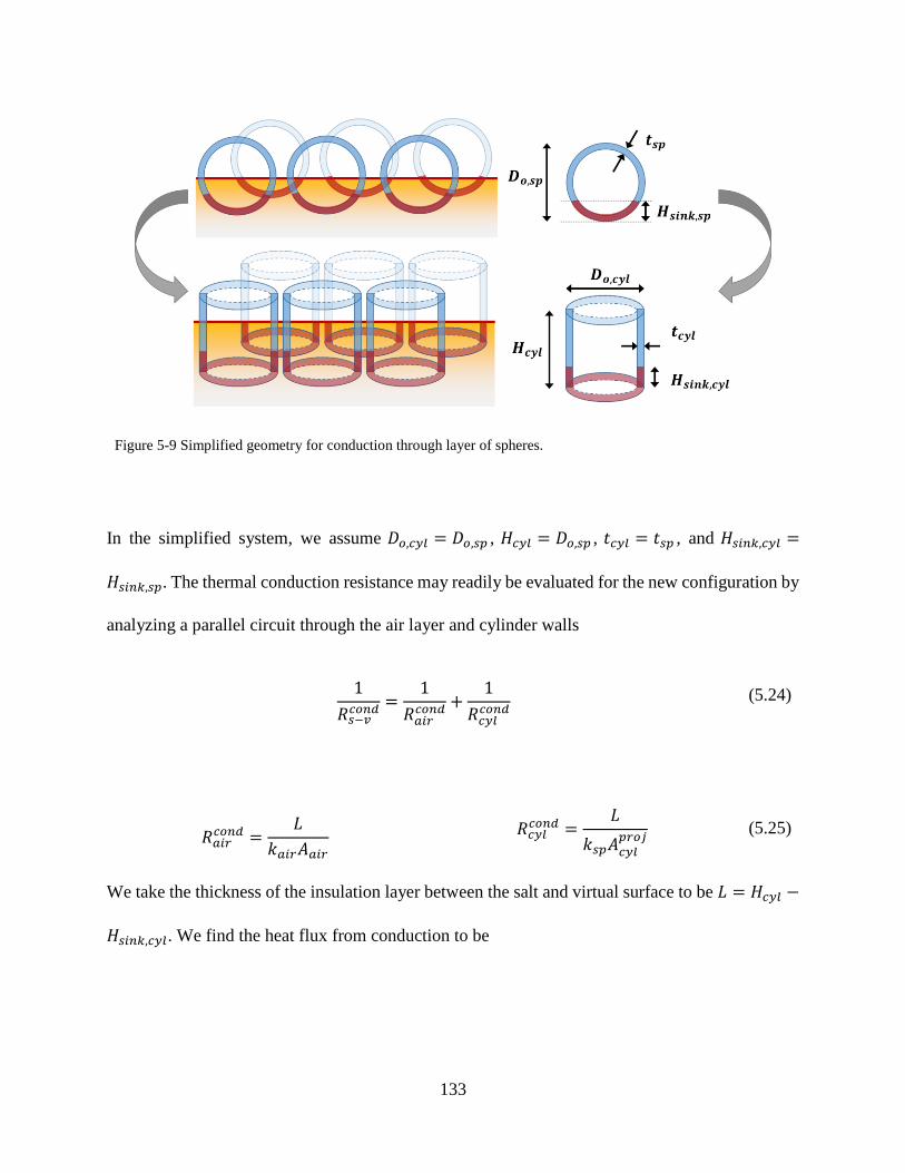
5.2. Methodology ................................................................................................................ 118

5.2.1. Laboratory experiments and simulation validation............................................... 119

5.2.2. Large scale molten salt solar pond performance................................................... 129

5.2.3. Solar pond capture efficiency ............................................................................... 139

5.3. Analysis of receiver heat loss mechanisms .................................................................. 140

11

5.3.1. Convection ............................................................................................................ 140

5.3.2. Radiation ............................................................................................................... 142

5.3.3. Evaporation ........................................................................................................... 142

5.3.4. Magnitude Comparison ......................................................................................... 142

5.4. Discussion .................................................................................................................... 145

5.5. Conclusions .................................................................................................................. 149

6. Concluding Remarks ........................................................................................................... 150

6.1. Conclusions .................................................................................................................. 150

6.2. Future Work ................................................................................................................. 153

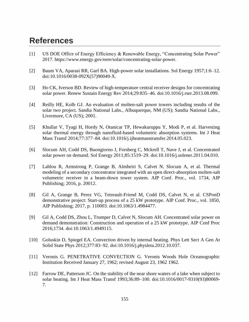
References ................................................................................................................................... 155

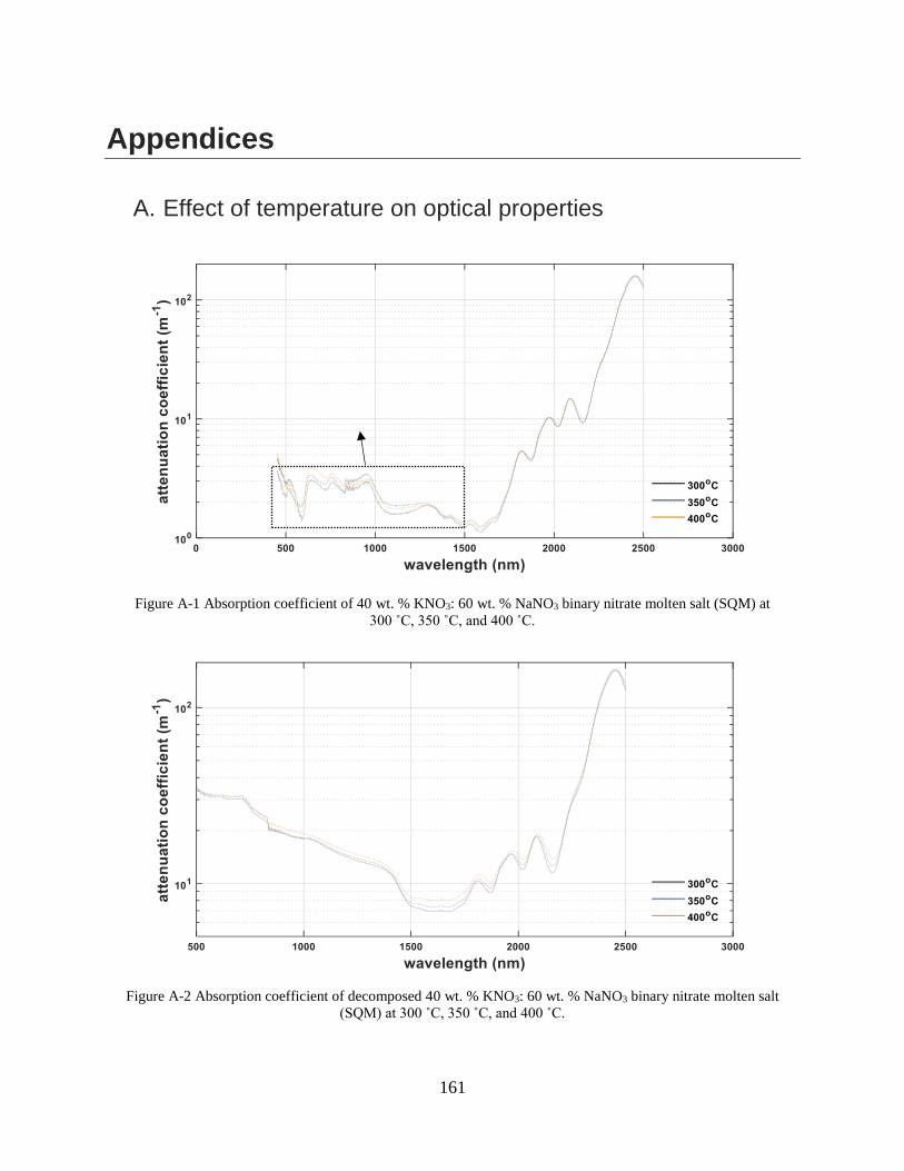
Appendices .................................................................................................................................. 161

A. Effect of temperature on optical properties ........................................................................ 161

B. Uncertainty analysis in optical property measurements ..................................................... 162

C. Reflectance calculation ....................................................................................................... 163

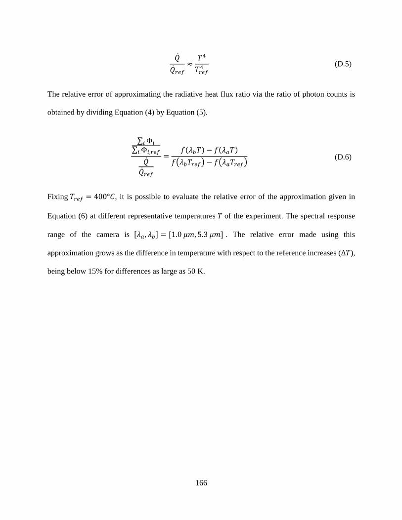
D. Conversion of photon counts to heat flux ratio ................................................................... 165

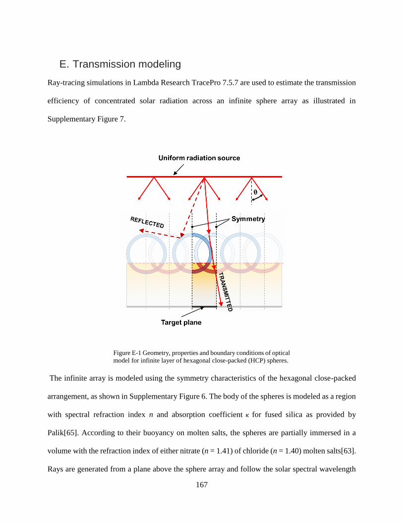
E. Transmission modeling ....................................................................................................... 167

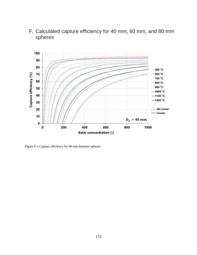
F. Calculated capture efficiency for 40 mm, 60 mm, and 80 mm spheres.............................. 172

G. Thermophysical properties of SQM Solar Salt ................................................................... 175

H. Divider plate and mixing plate designs ............................................................................... 176

12

List of Figures

Figure 1-1 Cross-section of the general CSPonD molten salt receiver concept during (a) on-sun

operation at the end of the day, and (b) after a prolonged period with continued heat extraction but

without solar heating. .................................................................................................................... 21

Figure 1-2 (a) Photo and (b) simplified diagram of the CSPonD demonstration facility. ............ 23

Figure 1-3 (a) Illustration of the expected thermal behaviour inside the receiver. The internal

heating produces two layers in the receiver: a thermally stratified and stagnant upper layer, and an

unstable bottom mixing layer. The semi-transparent hot salt. (b) Illustration of a re-emitting

participating media........................................................................................................................ 27

Figure 1-4 Ideal Carnot heat engine and associated maximum thermal efficiency based on oK.

Increasing the maximum operating temperature TH using high temperature liquids such as molten

salts allows to increase the maximum possible heat engine efficiency. ....................................... 29

Figure 1-5 Illustration summarizing the four principal thermal-fluid topics investigated in this

thesis. ............................................................................................................................................ 34

Figure 2-1. Simplified diagram of apparatus used to measure the attenuation of light intensity by

liquids. ........................................................................................................................................... 37

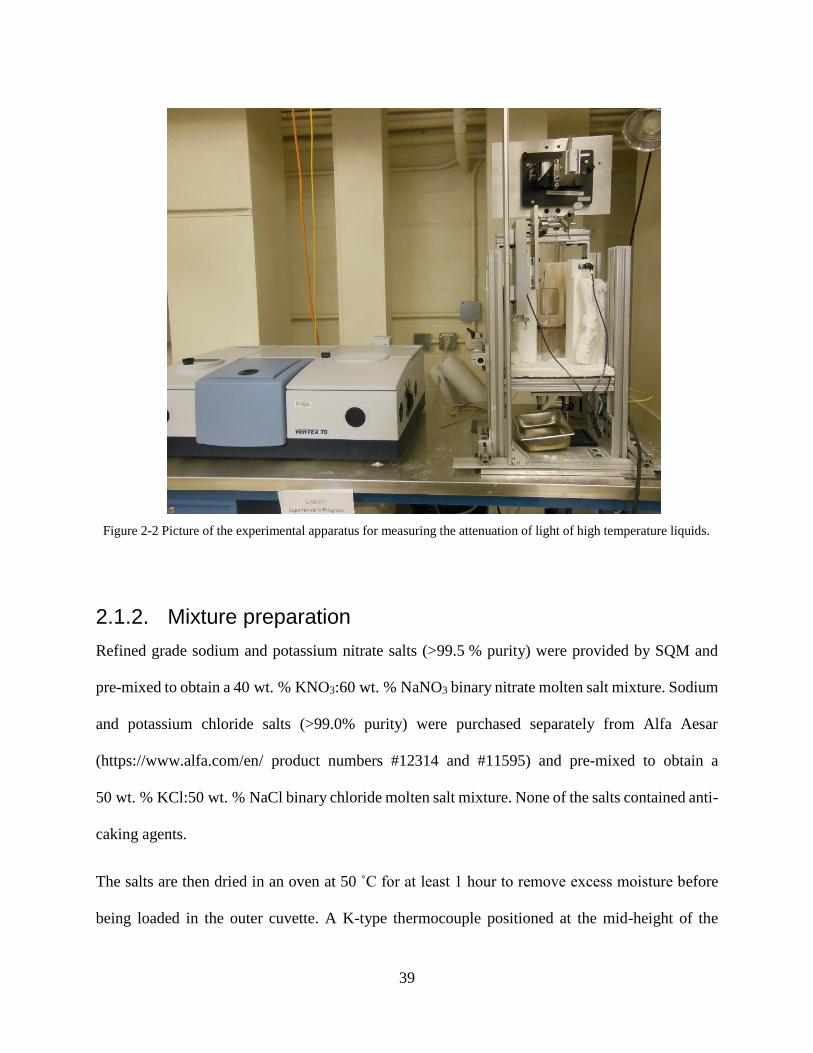
Figure 2-2 Picture of the experimental apparatus for measuring the attenuation of light of high

temperature liquids........................................................................................................................ 39

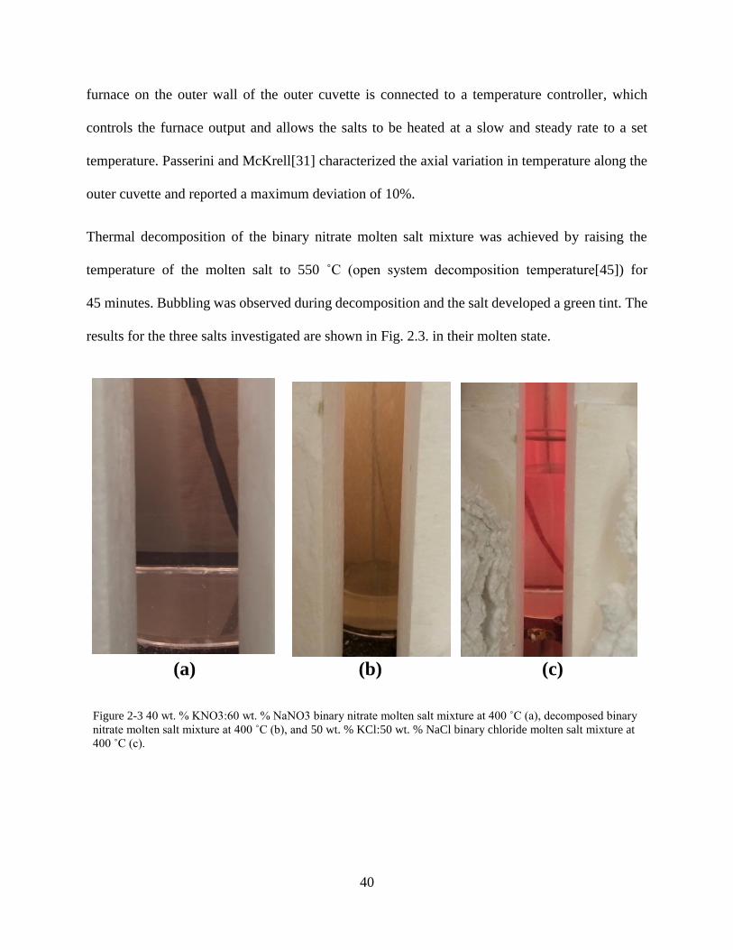
Figure 2-3 40 wt. % KNO3:60 wt. % NaNO3 binary nitrate molten salt mixture at 400 ˚C (a),

decomposed binary nitrate molten salt mixture at 400 ˚C (b), and 50 wt. % KCl:50 wt. % NaCl

binary chloride molten salt mixture at 400 ˚C (c). ........................................................................ 40

Figure 2-4 Diagram illustrating assumptions and boundary conditions for performance evaluation.

....................................................................................................................................................... 44

Figure 2-5 Experimental results for the attenuation coefficient of propylene glycol versus

wavelength. ................................................................................................................................... 45

Figure 2-6 Attenuation Coefficient of 40 wt. % KNO3: 60 wt. % NaNO3 binary nitrate molten salt

(SQM) at 400 ˚C. .......................................................................................................................... 46

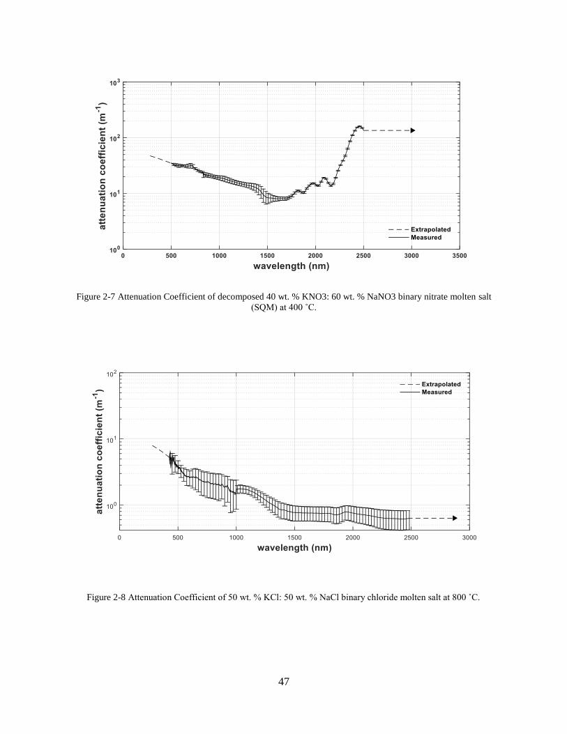
Figure 2-7 Attenuation Coefficient of decomposed 40 wt. % KNO3: 60 wt. % NaNO3 binary

nitrate molten salt (SQM) at 400 ˚C. ............................................................................................ 47

Figure 2-8 Attenuation Coefficient of 50 wt. % KCl: 50 wt. % NaCl binary chloride molten salt at

800 ˚C............................................................................................................................................ 47

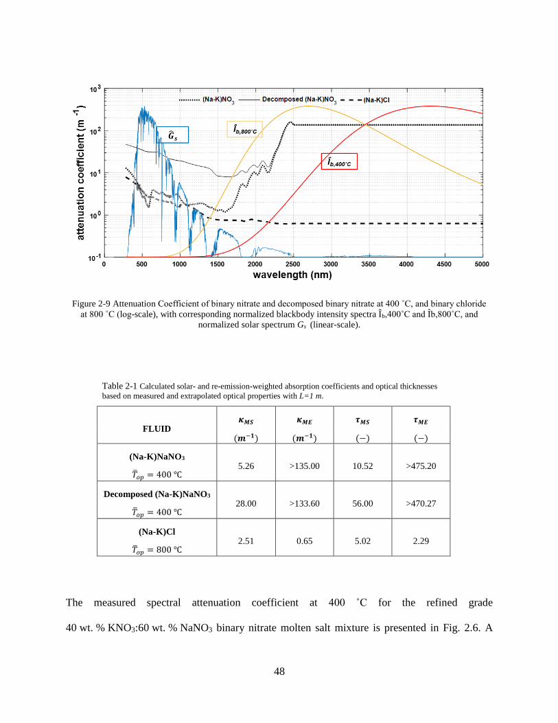
Figure 2-9 Attenuation Coefficient of binary nitrate and decomposed binary nitrate at 400 ˚C, and

binary chloride at 800 ˚C (log-scale), with corresponding normalized blackbody intensity spectra

Îb,400˚C and Îb,800˚C, and normalized solar spectrum Gs (linear-scale)..................................... 48

Figure 2-10 Solar irradiance distribution at different salt depths for binary nitrate at 400 ˚C. .... 51

Figure 2-11 Solar irradiance distribution at different salt depths for binary chloride at 800 ˚C. . 52

13

Figure 2-12 Effective total emissivity of measured molten salt mixtures for different receiver fluid

depths. ........................................................................................................................................... 53

Figure 2-13 Capture efficiency versus solar concentrations for fluid depths between 0.25 m and 2

m for binary nitrate (a), decomposed binary nitrate (b), and binary chloride (c). ........................ 56

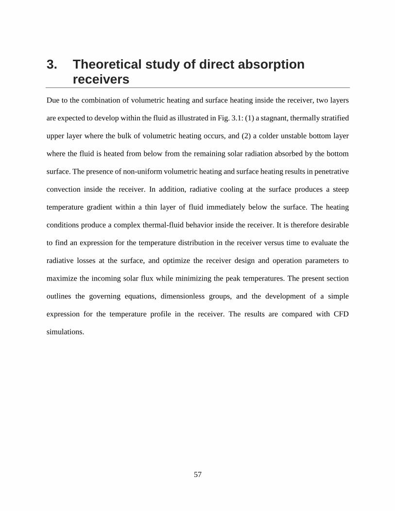
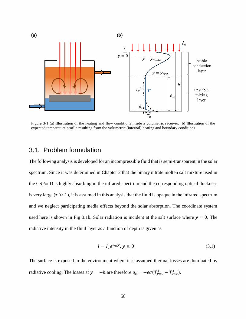
Figure 3-1 (a) Illustration of the heating and flow conditions inside a volumetric receiver. (b)

Illustration of the expected temperature profile resulting from the volumetric (internal) heating and

boundary conditions. ..................................................................................................................... 58

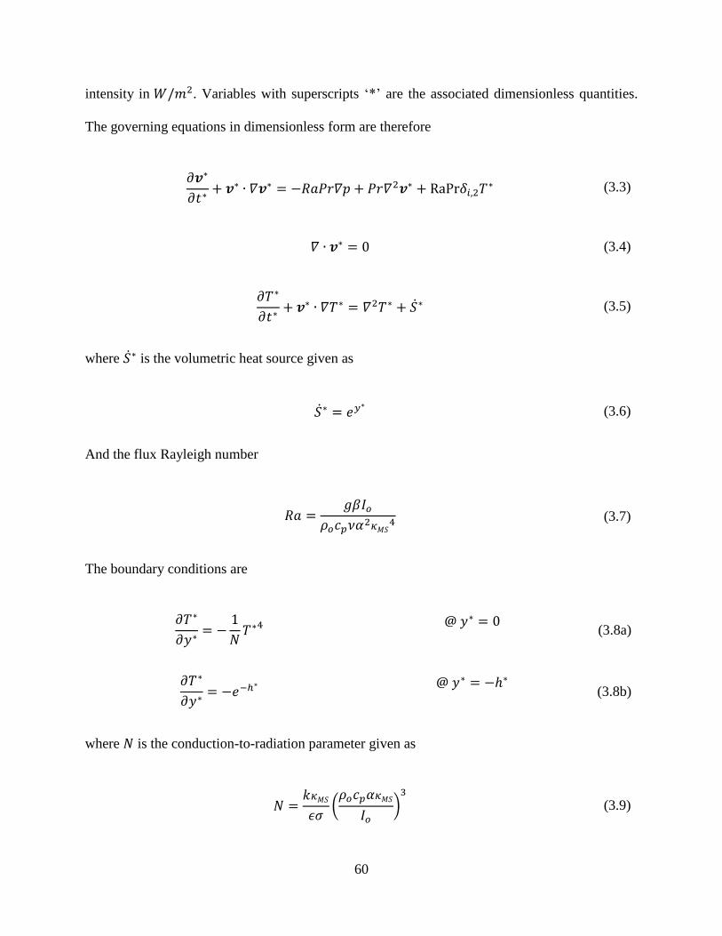
Figure 3-2 Illustration of the modelled region in CFD for validation of the 1D model. Lateral walls

are defined as symmetry planes such that the region is semi-infinite in the xz-plane. ................. 65

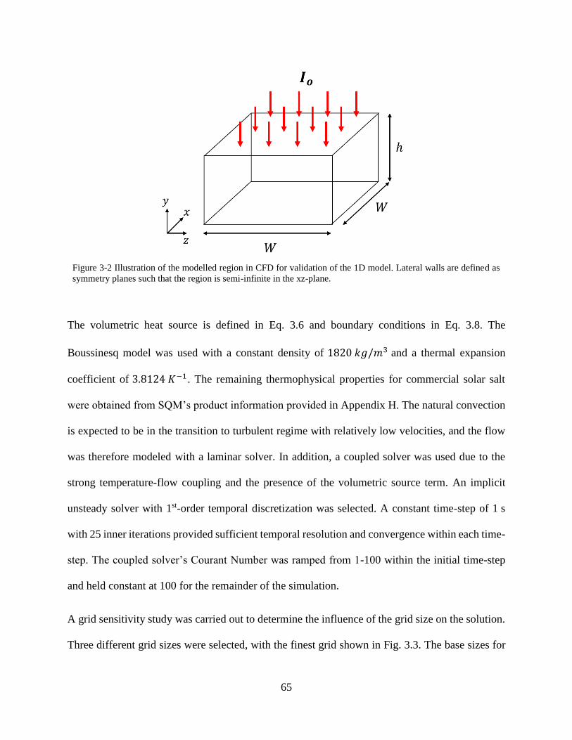
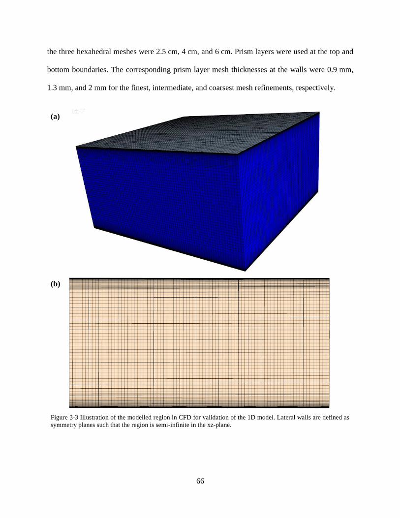
Figure 3-3 Illustration of the modelled region in CFD for validation of the 1D model. Lateral walls

are defined as symmetry planes such that the region is semi-infinite in the xz-plane. ................. 66

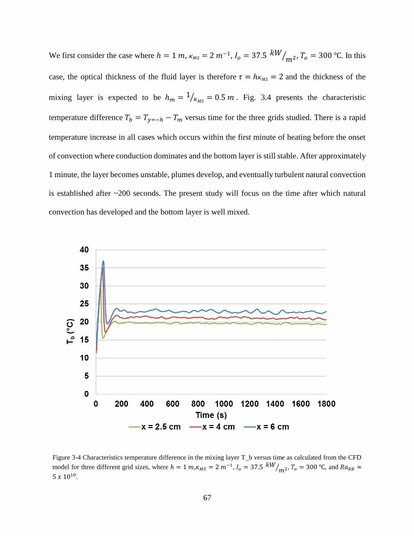
Figure 3-4 Characteristics temperature difference in the mixing layer T_b versus time as calculated

from the CFD model for three different grid sizes, where ℎ = 1 𝑚 , 𝜅𝑀𝑆 = 2 𝑚−1 , 𝐼𝑜 =37.5 𝑘𝑊/𝑚2, 𝑇𝑜 = 300 ℃, and 𝑅𝑎𝑅𝐵 ≈ 5 𝑥 1010. ..................................................................... 67

Figure 3-5 Axial temperature profile in an internally heated liquid layer calculated with the simple

1D model and the CFD model for ℎ = 1 𝑚, 𝜅𝑀𝑆 = 2 𝑚−1, 𝐼𝑜 = 37.5 𝑘𝑊/𝑚2, 𝑇𝑜 = 300 ℃, and 𝑅𝑎𝑅𝐵 ≈ 5 𝑥 1010........................................................................................................................... 69

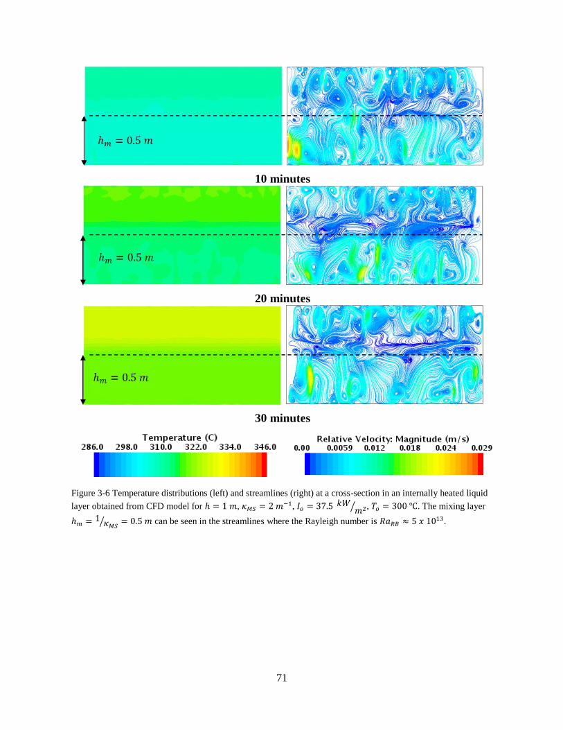
Figure 3-6 Temperature distributions (left) and streamlines (right) at a cross-section in an internally

heated liquid layer obtained from CFD model for ℎ = 1 𝑚 , 𝜅𝑀𝑆 = 2 𝑚−1 , 𝐼𝑜 = 37.5 𝑘𝑊/𝑚2 , 𝑇𝑜 = 300 ℃, and 𝑅𝑎𝑅𝐵 ≈ 5 𝑥 1010. . .......................................................................................... 71

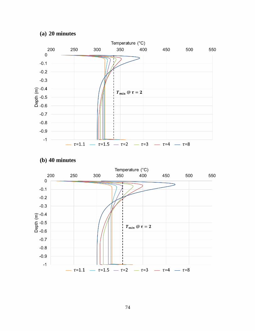
Figure 3-7 Variation of the temperature profile with optical thickness calculated using the 1D

model for the case ℎ = 1 𝑚, 𝐼𝑜 = 𝑘𝑊/𝑚2, 𝑇𝑜 = 300 ℃, with absorption coefficient ranging from

𝜅𝑀𝑆 = 1.1 𝑚−1 to 𝜅𝑀𝑆 = 8 𝑚−1 such that the optical thickness 𝜏 = 𝜅𝑀𝑆ℎ varies from 1.1 to 8.

Temperature profiles for heating times of (a) 20 minutes, (b) 40 minutes, and (c) 60 minutes. .. 75

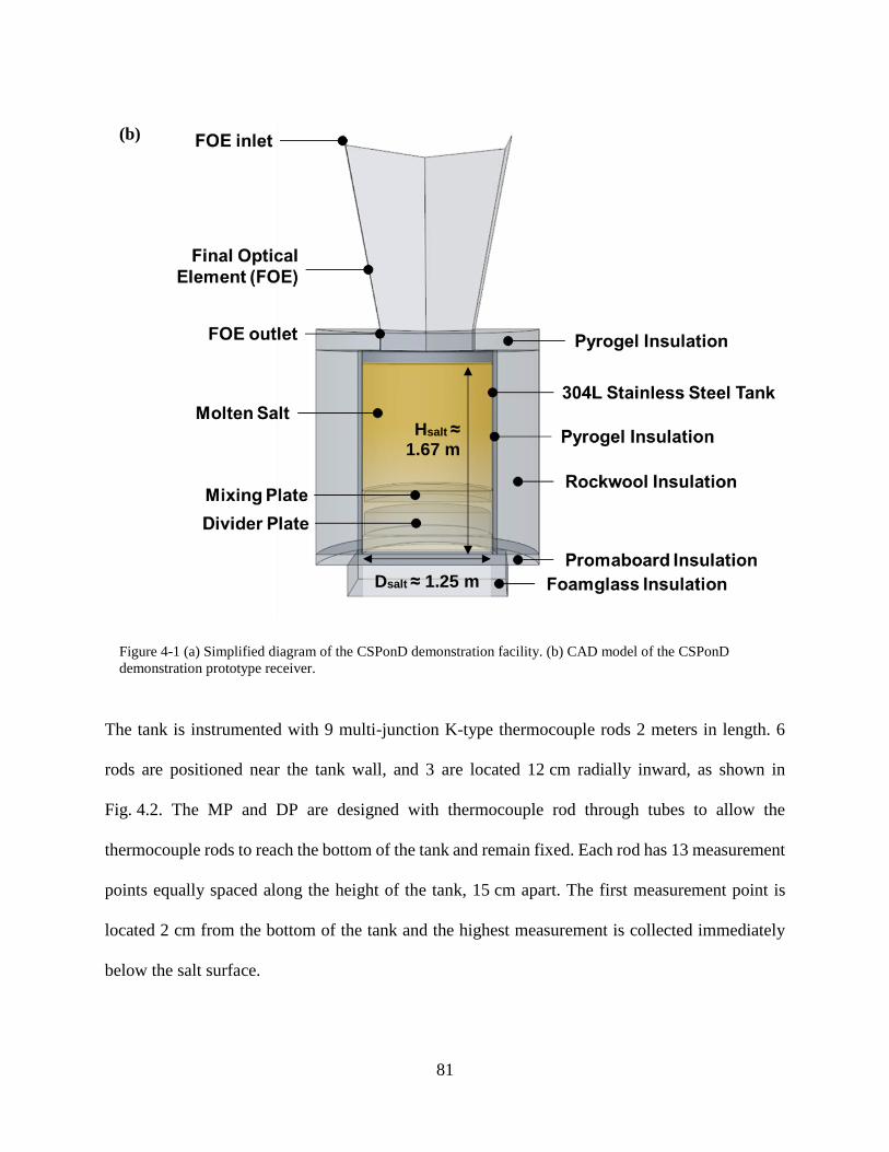
Figure 4-1 (a) Simplified diagram of the CSPonD demonstration facility. (b) CAD model of the

CSPonD demonstration prototype receiver. ................................................................................. 81

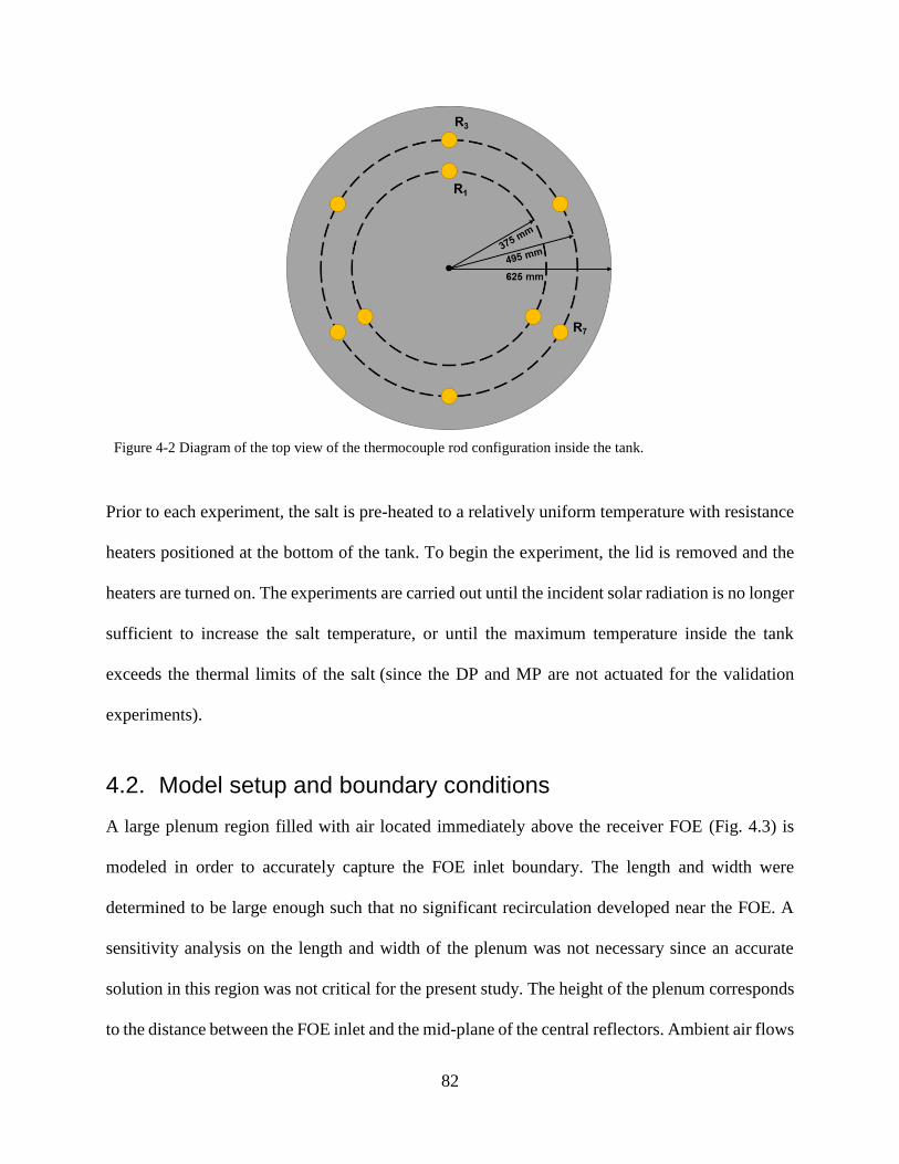
Figure 4-2 Diagram of the top view of the thermocouple rod configuration inside the tank. ...... 82

Figure 4-3 Model setup and boundary conditions (plenum not to scale). .................................... 83

Figure 4-4 Distribution of the incident solar irradiation on the final optical element (FOE) for S4,

S6, S8 ordinates discretization. ...................................................................................................... 88

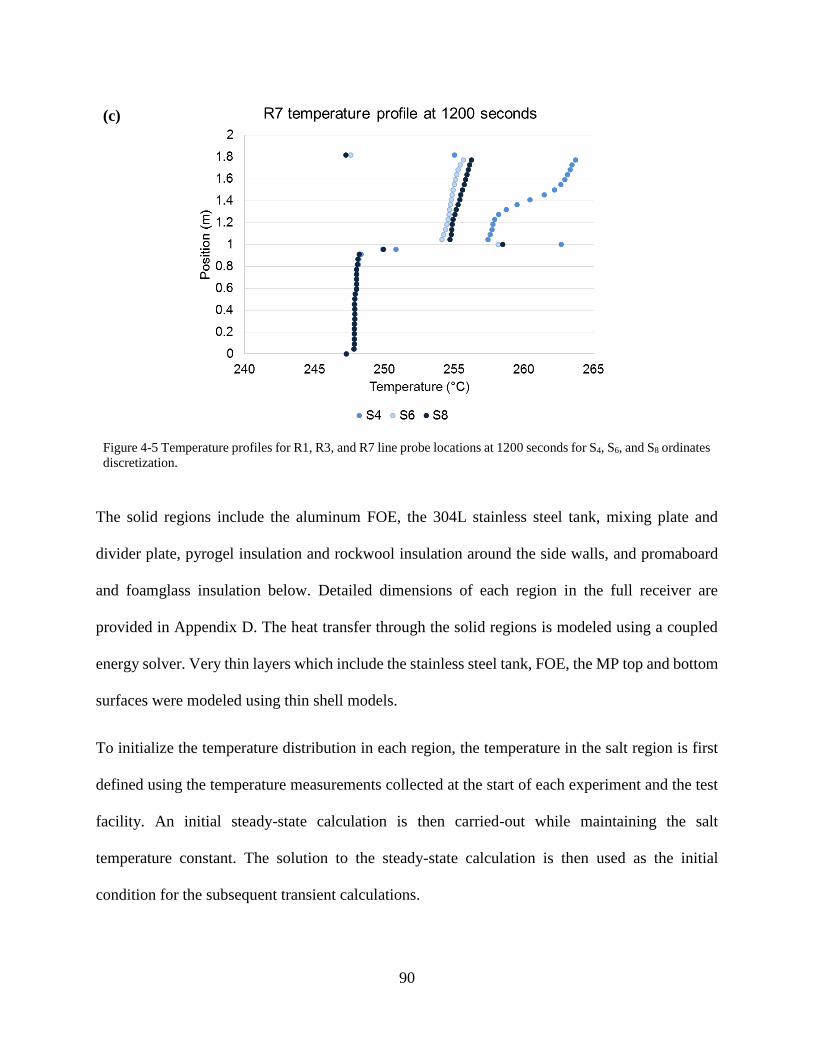
Figure 4-5 Temperature profiles for R1, R3, and R7 line probe locations at 600 seconds for S4, S6,

and S8 ordinates discretization. ..................................................................................................... 90

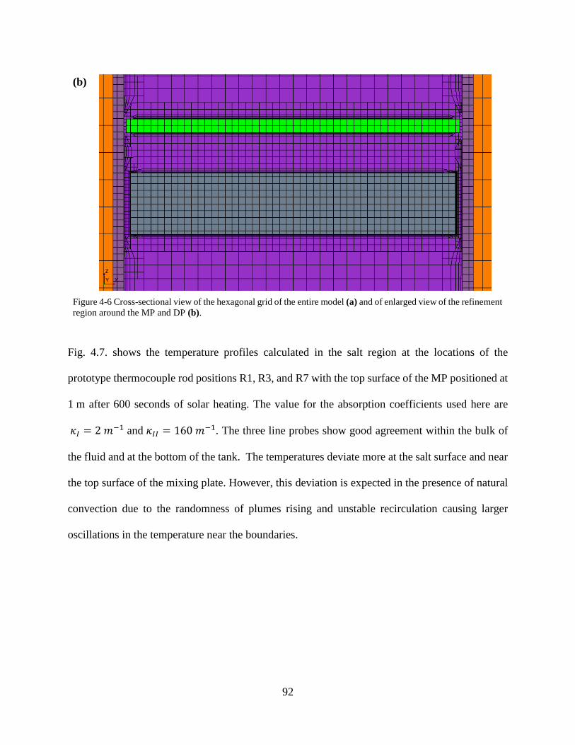
Figure 4-6 Cross-sectional view of the hexagonal grid of the entire model (a) and of enlarged view

of the refinement region around the MP and DP (b). ................................................................... 92

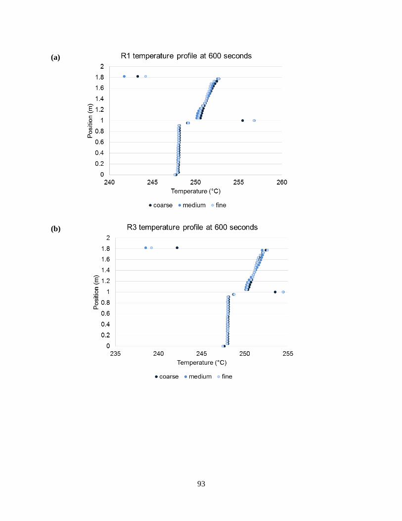
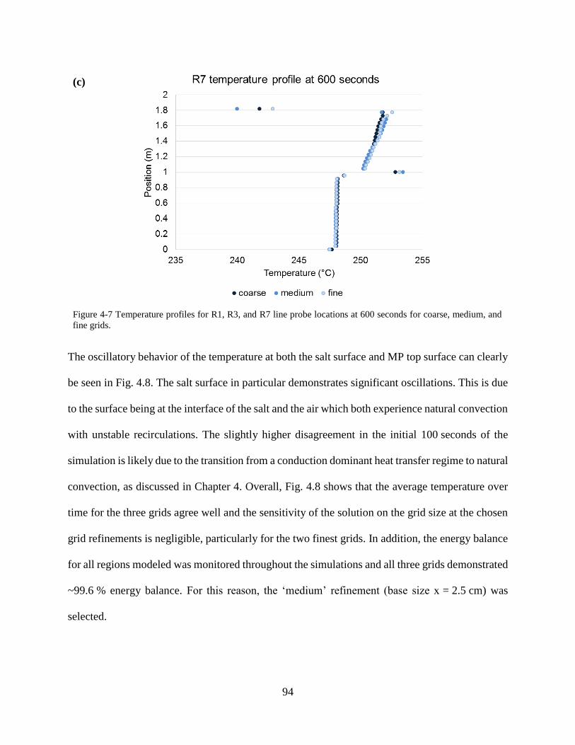
Figure 4-7 Temperature profiles for R1, R3, and R7 line probe locations at 600 seconds for coarse,

medium, and fine grids. ................................................................................................................ 94

14

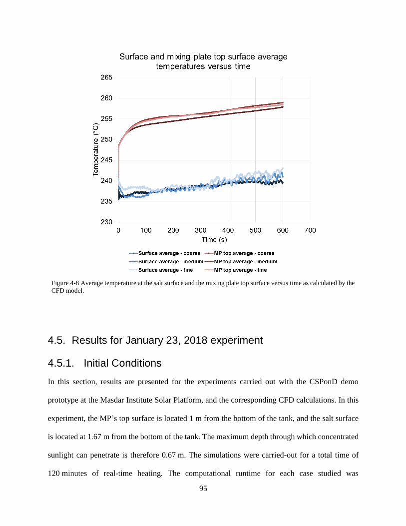
Figure 4-8 Average temperature at the salt surface and the mixing plate top surface versus time as

calculated by the CFD model. ....................................................................................................... 95

Figure 4-9 Solar flux bottom output as estimated using ray-tracing [62] and corresponding

polynomial interpolation used as input for the CFD calculations................................................. 96

Figure 4-10 Initial surface irradiation on FOE, salt surface, and MP for spectral band I (solar

spectral band). ............................................................................................................................... 97

Figure 4-11 Initial temperature and velocity distribution for all cases studied. ........................... 98

Figure 4-12 Cross-sectional temperature distribution of all modeled regions after 60 minutes of

solar heating. ................................................................................................................................. 99

Figure 4-13 Temperature distribution of salt cross-section, salt surface, and MP surface after 60

minutes of solar heating. ............................................................................................................. 100

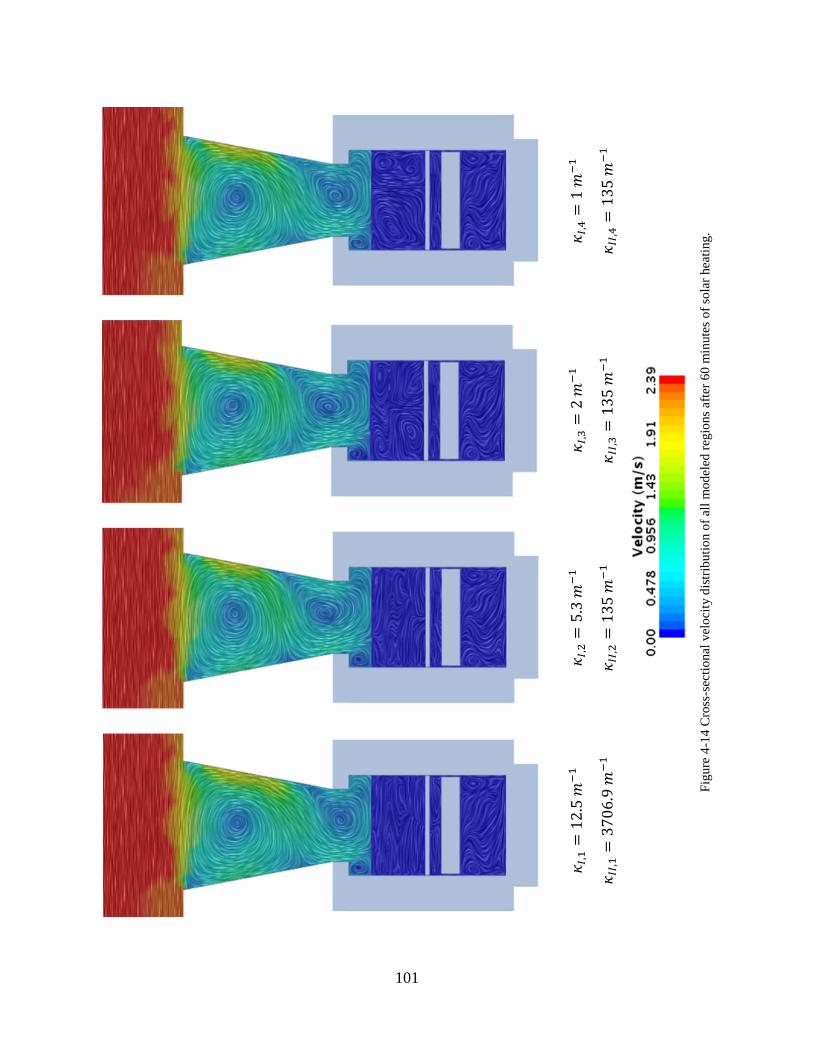
Figure 4-14 Cross-sectional velocity distribution of all modeled regions after 60 minutes of solar

heating. ........................................................................................................................................ 101

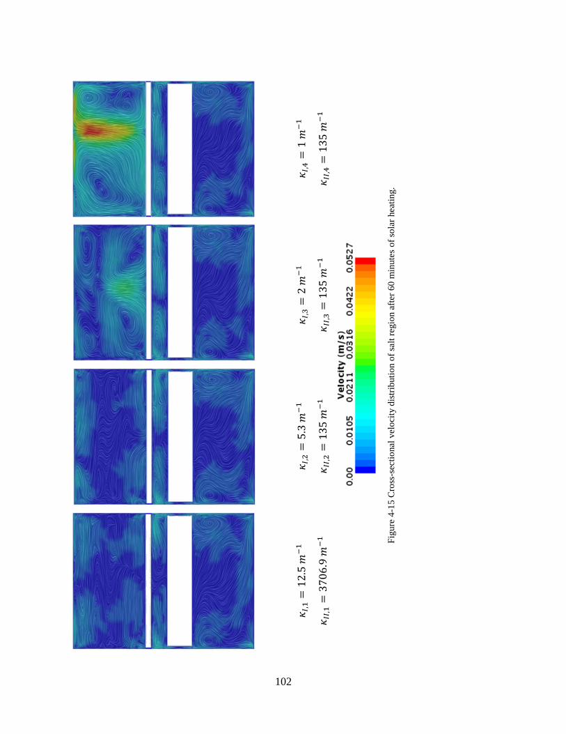
Figure 4-15 Cross-sectional velocity distribution of salt region after 60 minutes of solar heating.

..................................................................................................................................................... 102

Figure 4-16 Temperature profiles at location R1 for case 𝜅𝐼,1 = 12.5 𝑚 − 1, 𝜅𝐼𝐼,1 = 3706.9 𝑚 −1 .................................................................................................................................................. 103

Figure 4-17 Temperature profiles at location R1 for case 𝜅𝐼,2 = 5.3 𝑚 − 1,𝜅𝐼𝐼,2 = 135 𝑚 − 1104

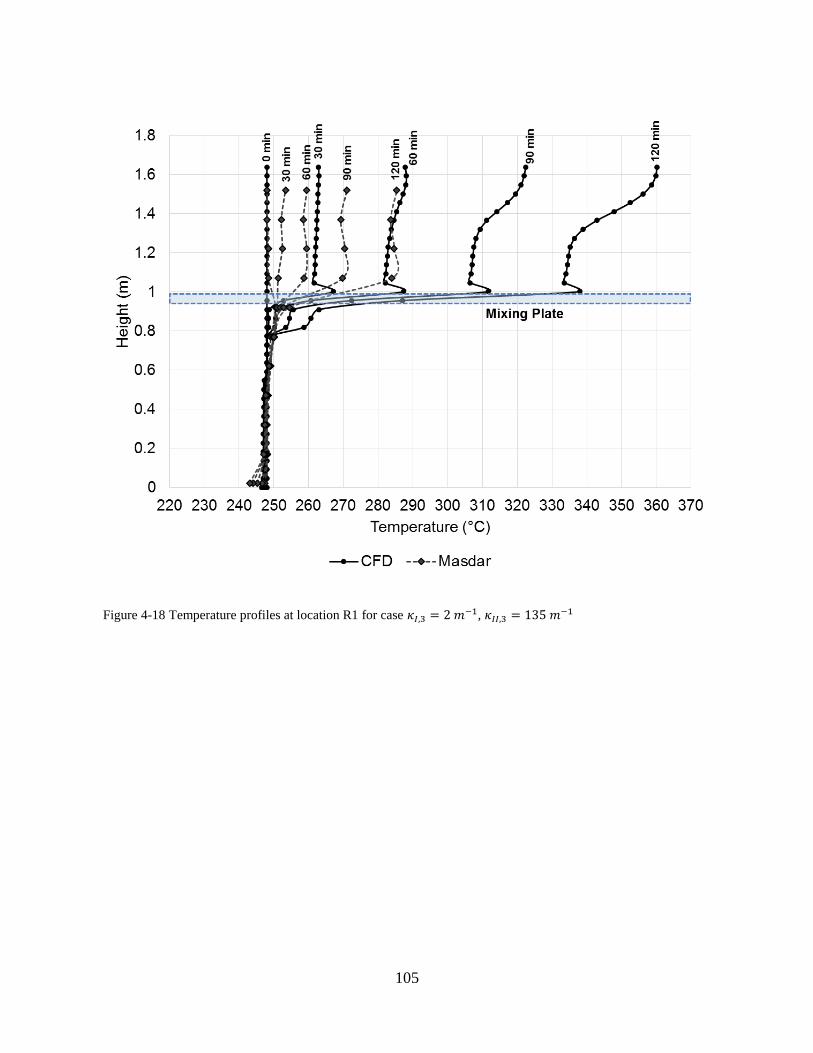
Figure 4-18 Temperature profiles at location R1 for case 𝜅𝐼,3 = 2 𝑚 − 1, 𝜅𝐼𝐼,3 = 135 𝑚 − 1 . 105

Figure 4-19 Temperature profiles at location R1 for case 𝜅𝐼,4 = 1 𝑚 − 1, 𝜅𝐼𝐼,4 = 135 𝑚 − 1 . 106

Figure 5-1 Solar pond energy balance and cover concept. ......................................................... 117

Figure 5-2 Validation experiment. Simplified diagram of the experimental setup used for

evaluating the thermal insulation performance of the floating spheres, and 3D representation of the

simulated section. An infrared camera is used to measure the photon flux losses from the surface

of a heated beaker filled with molten salt, with and without floating spheres............................ 120

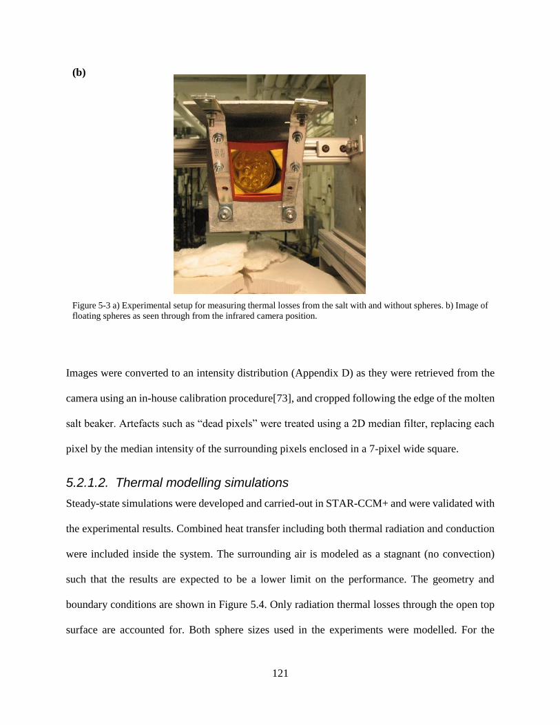
Figure 5-3 a) Experimental setup for measuring thermal losses from the salt with and without

spheres. b) Image of floating spheres as seen through from the infrared camera position. ........ 121

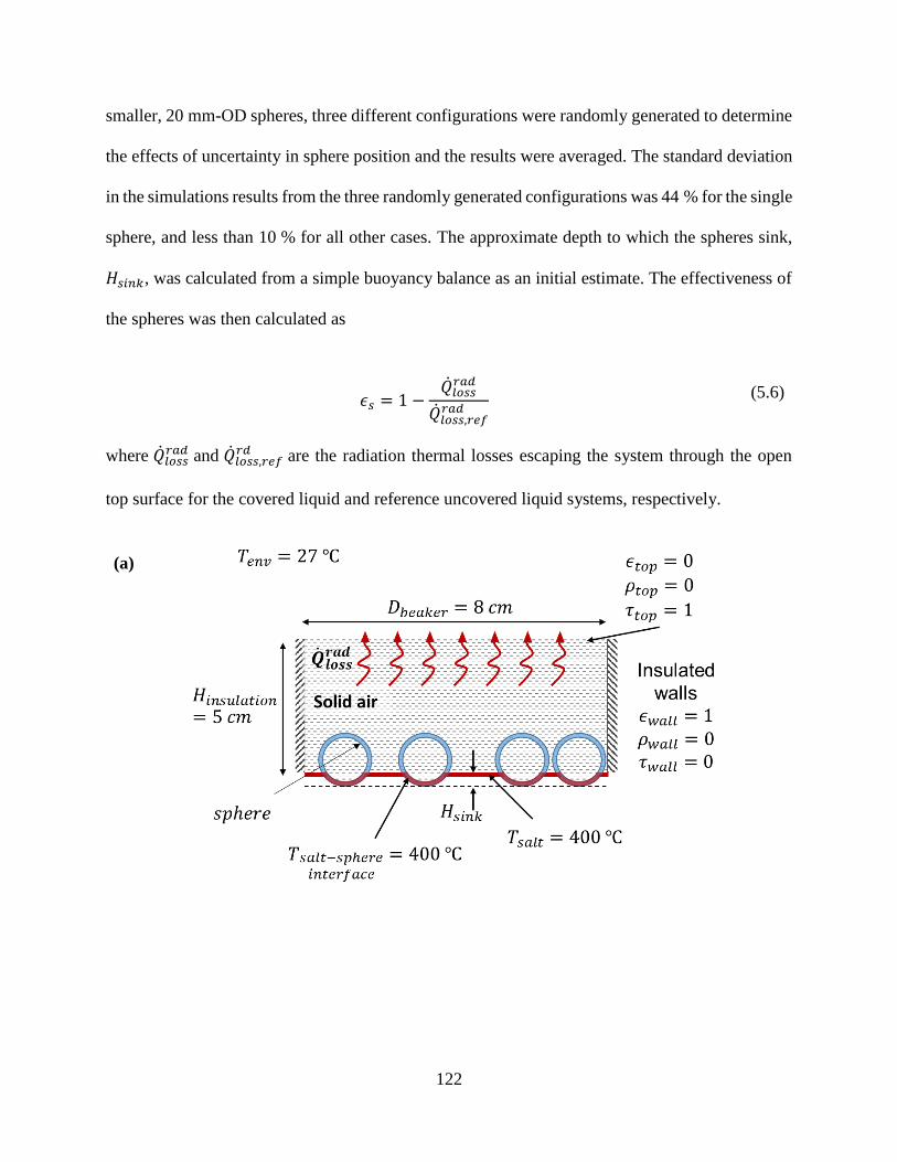
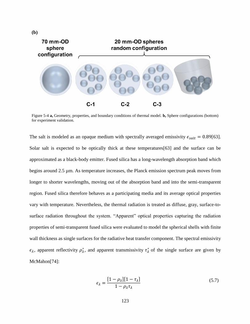
Figure 5-4 a, Geometry, properties, and boundary conditions of thermal model. b, Sphere

configurations (bottom) for experiment validation. .................................................................... 123

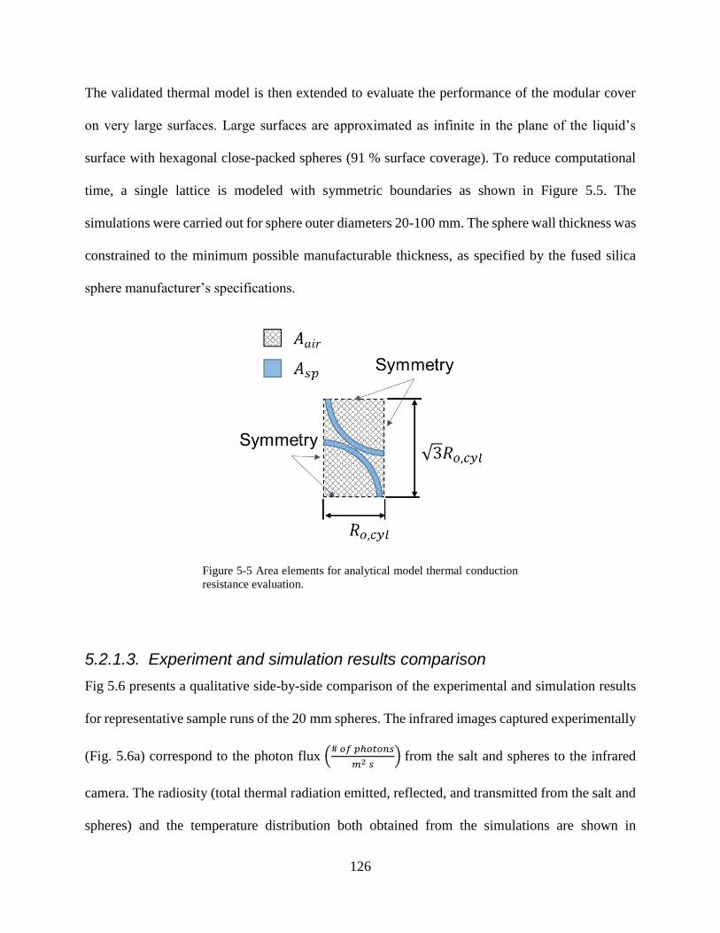
Figure 5-5 Area elements for analytical model thermal conduction resistance evaluation. ....... 126

Figure 5-6 Validation experiment and simulation results. a, Photon flux map to infrared camera

obtained experimentally. Radiosity (b) and temperature distribution (c) at salt and sphere surfaces

calculated numerically. d, Calculated thermal effectiveness of floating spheres versus surface

coverage in laboratory scale experiment and validation simulation. .......................................... 128

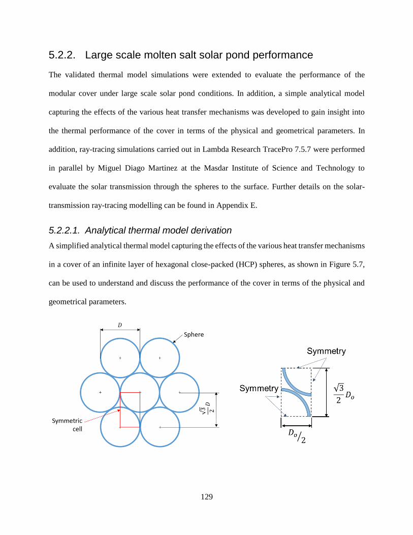
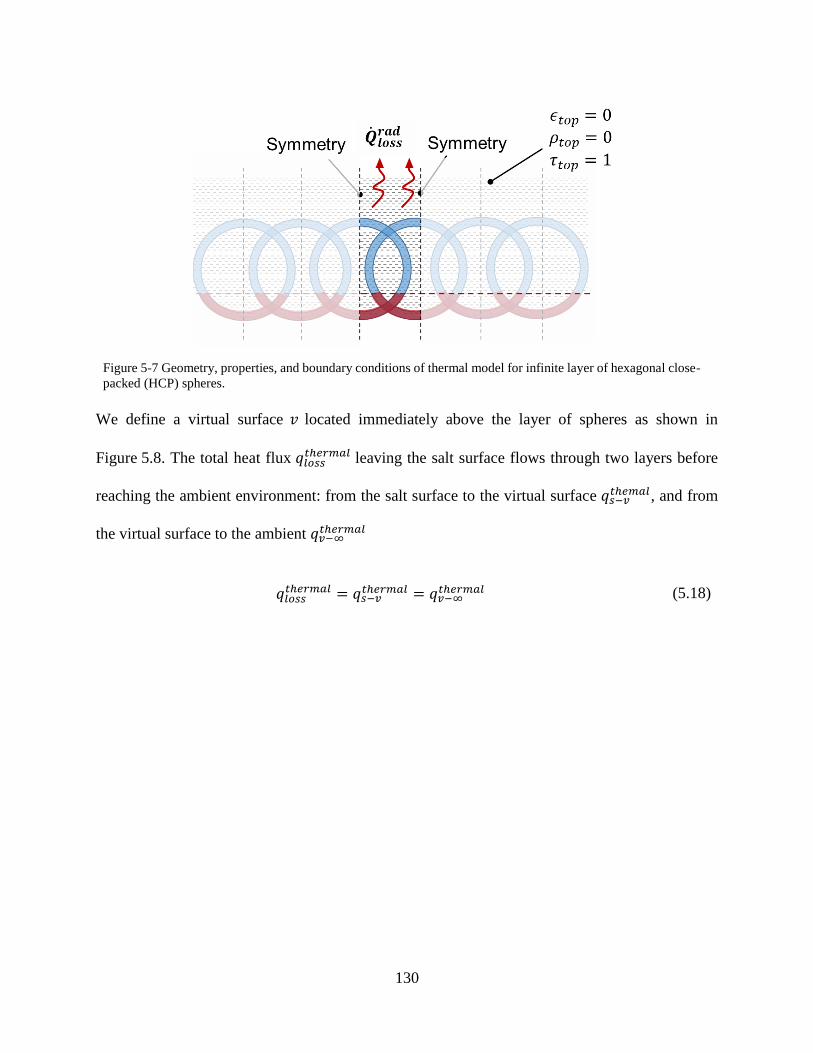
Figure 5-7 Geometry, properties, and boundary conditions of thermal model for infinite layer of

hexagonal close-packed (HCP) spheres. ..................................................................................... 130

15

Figure 5-8 Diagram illustrating the simplified analytical model. ............................................... 131

Figure 5-9 Simplified geometry for conduction through layer of spheres. ................................. 133

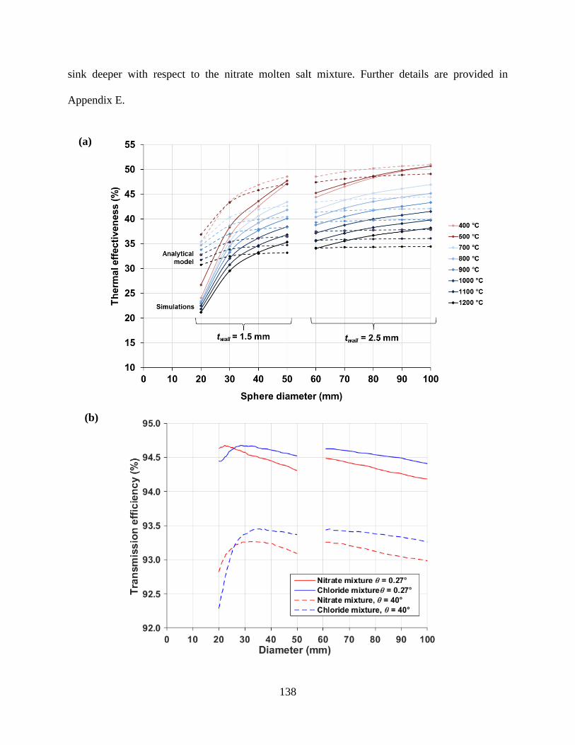
Figure 5-10 Thermal and transmission performance. a, Thermal effectiveness versus sphere

diameter. b, Transmission efficiency versus sphere diameter. Wall thicknesses in both (a) and (b)

are 1.5 mm for diameters 𝐷𝑜 ≤ 50 𝑚𝑚, and 2.5 mm for diameters 𝐷𝑜 ≥ 60 𝑚𝑚, as specified by

fused silica manufacturer. Transmission calculations and figures were carried out and prepared by

Miguel Diago Martinez. .............................................................................................................. 139

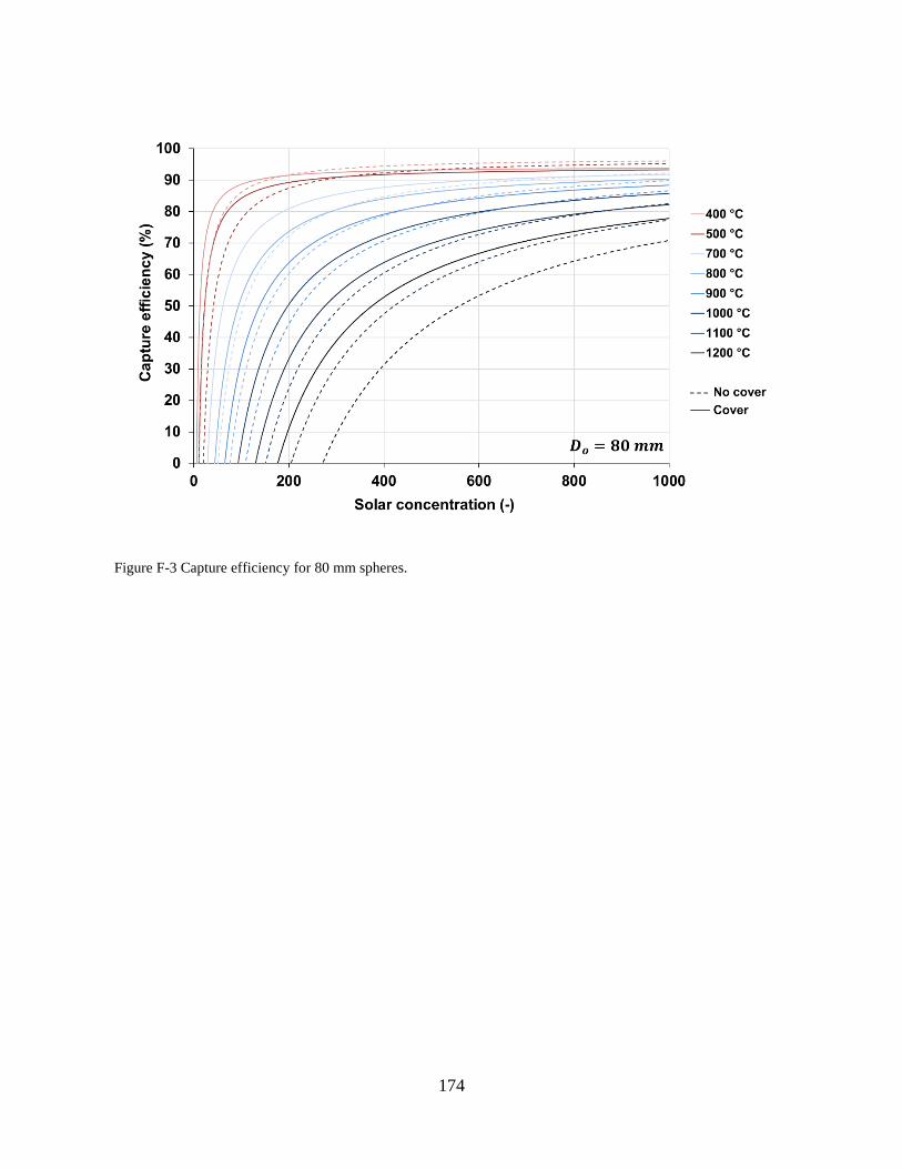
Figure 5-11 Solar pond capture efficiency. Capture efficiency of solar pond with densely packed

HCP cover for 𝐷𝑜 = 20 𝑚𝑚 (a) and 𝐷𝑜 = 100 𝑚𝑚 spheres (b), and with surface temperatures

between 400 °C - 500 °C for 40 wt. % KNO3:60 wt. % NaNO3 binary nitrate molten salt, and

700 °C - 1200 °C for 50 wt. % KCl:50 wt. % NaCl binary chloride molten salt. Dashed lines

represent capture efficiencies without a cover. ........................................................................... 140

Figure 5-12 Capture efficiency comparison between solar central receiver systems and volumetric

receiver for solar concentration C=300 (a) and C=600 (b). Solar central receiver data adapted from

Karni [80]. ................................................................................................................................... 147

Figure A-1 Absorption coefficient of 40 wt. % KNO3: 60 wt. % NaNO3 binary nitrate molten salt

(SQM) at 300 ˚C, 350 ˚C, and 400 ˚C........................................................................................ 161

Figure A-2 Absorption coefficient of decomposed 40 wt. % KNO3: 60 wt. % NaNO3 binary nitrate

molten salt (SQM) at 300 ˚C, 350 ˚C, and 400 ˚C. ..................................................................... 161

Figure E-1 Geometry, properties and boundary conditions of optical model for infinite layer of

hexagonal close-packed (HCP) spheres. ..................................................................................... 167

Figure E-2 Transmission efficiency on binary nitrate molten salt. a, Based on a sphere wall

thickness of 1 mm. b, More generally, as a function of the ratio of the sphere wall thickness to its

diameter....................................................................................................................................... 169

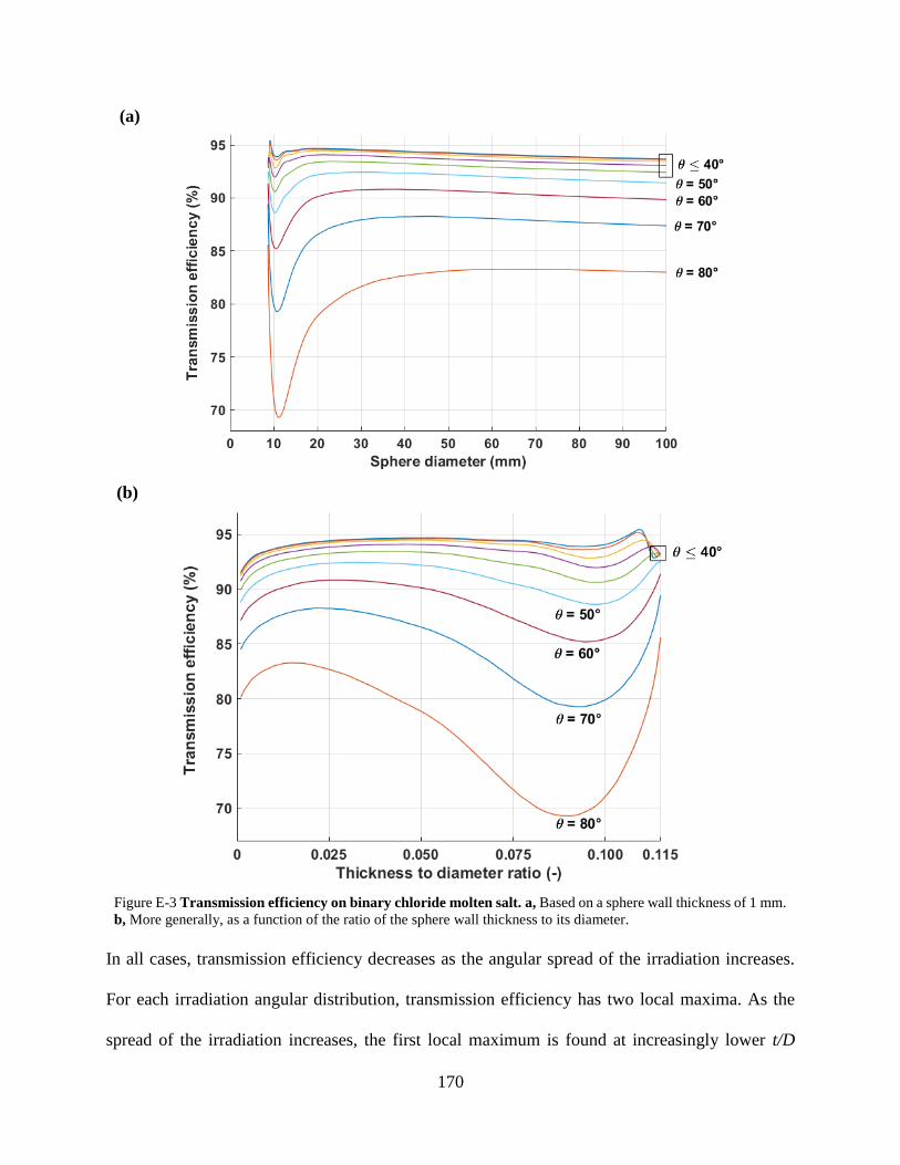
Figure E-3 Transmission efficiency on binary chloride molten salt. a, Based on a sphere wall

thickness of 1 mm. b, More generally, as a function of the ratio of the sphere wall thickness to its

diameter....................................................................................................................................... 170

Figure F-1 Capture efficiency for 40 mm diameter spheres. ...................................................... 172

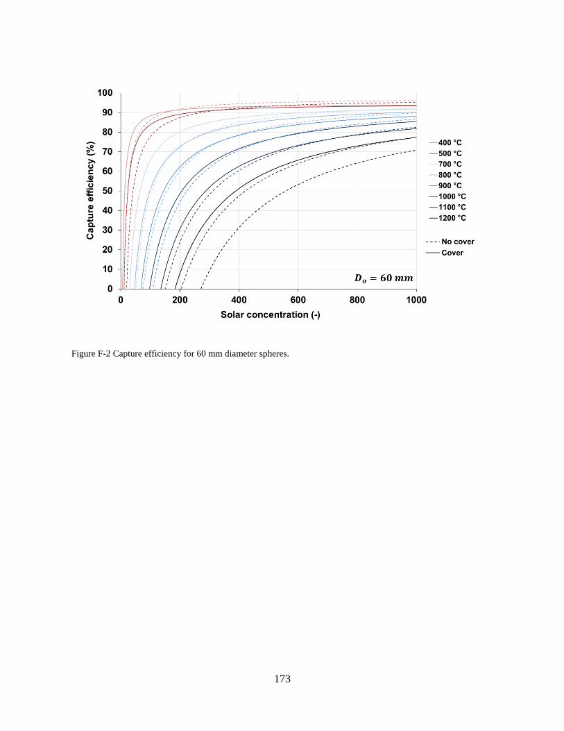
Figure F-2 Capture efficiency for 60 mm diameter spheres. ...................................................... 173

Figure F-3 Capture efficiency for 80 mm spheres. ..................................................................... 174

Figure H-1 Labelled cross-sectional views of the divider plate (a) and mixing plate (b) designs.

Adapted from Hamer et al. [61]. ................................................................................................. 176

Figure H-2 Equivalent thermal circuit for the axial conduction through the divider plate......... 176

16

List of Tables

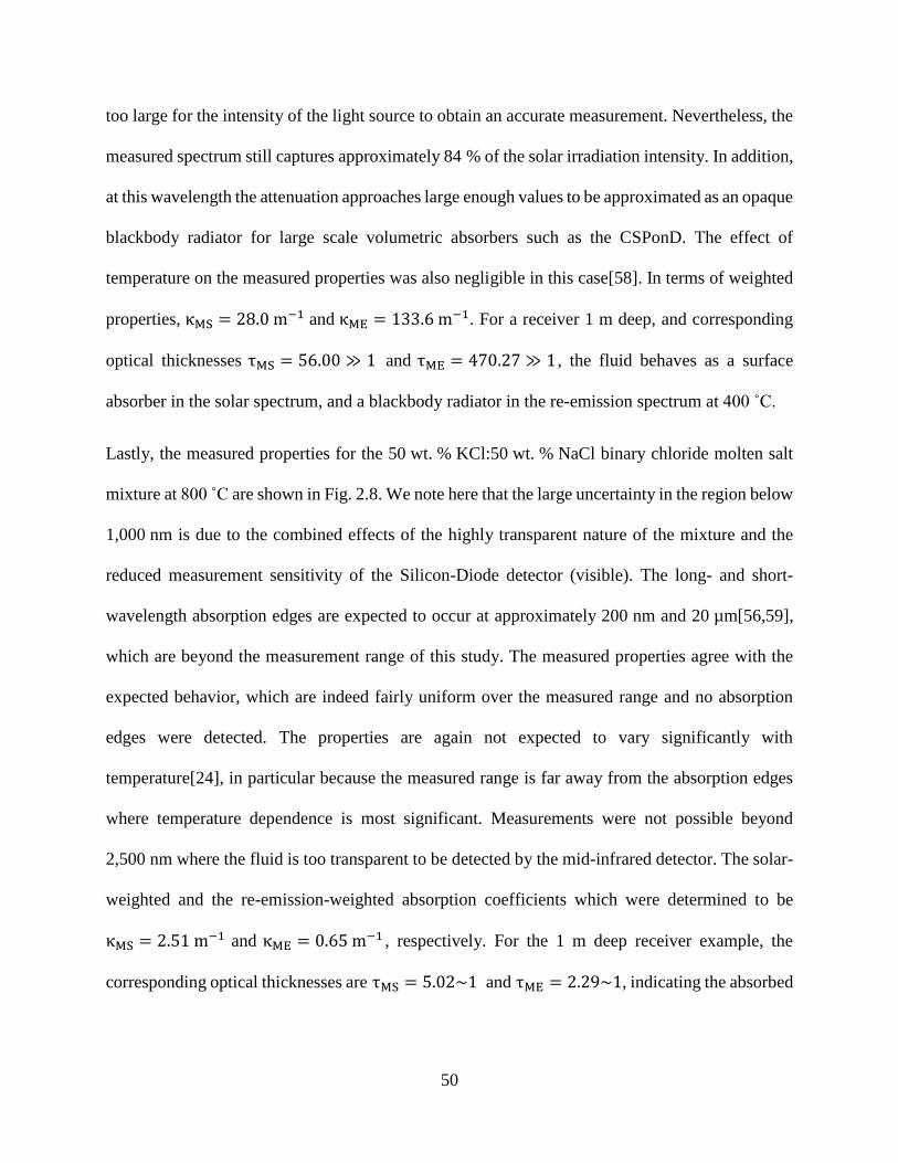
Table 2-1 Calculated solar- and re-emission-weighted absorption coefficients and optical

thicknesses based on measured and extrapolated optical properties with L=1 m......................... 48

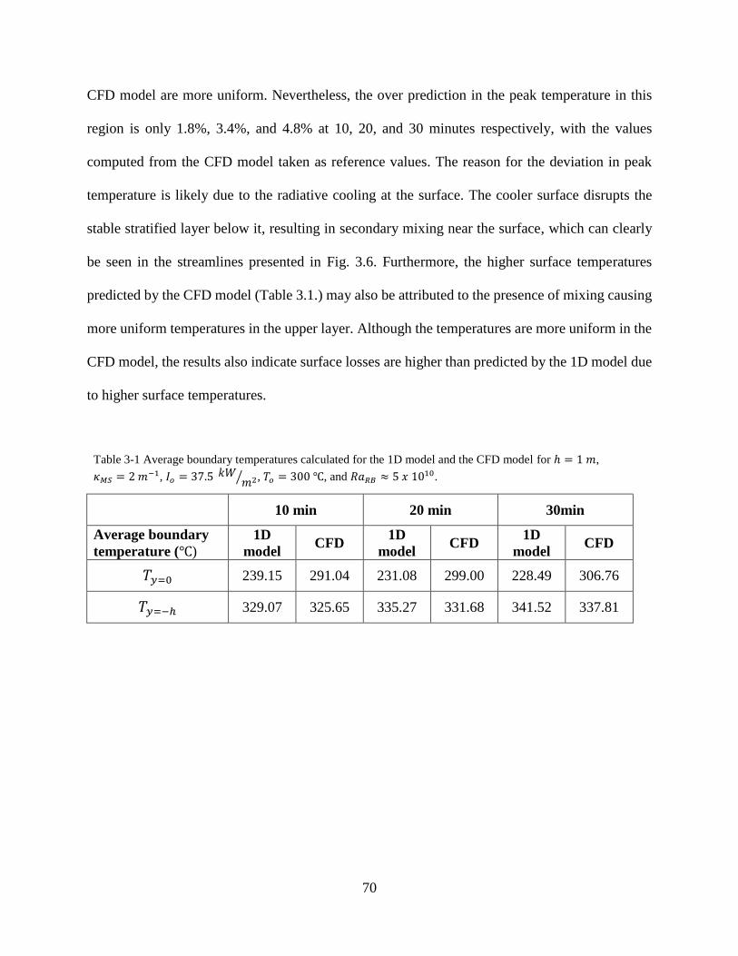
Table 3-1 Average boundary temperatures calculated for the 1D model and the CFD model for

ℎ = 1 𝑚, 𝜅𝑀𝑆 = 2 𝑚−1, 𝐼𝑜 = 37.5 𝑘𝑊/𝑚2, 𝑇𝑜 = 300 ℃, and 𝑅𝑎𝑅𝐵 ≈ 5 𝑥 1010. ..................... 70

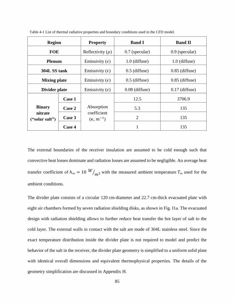
Table 4-1 List of thermal radiative properties and boundary conditions used in the CFD model.85

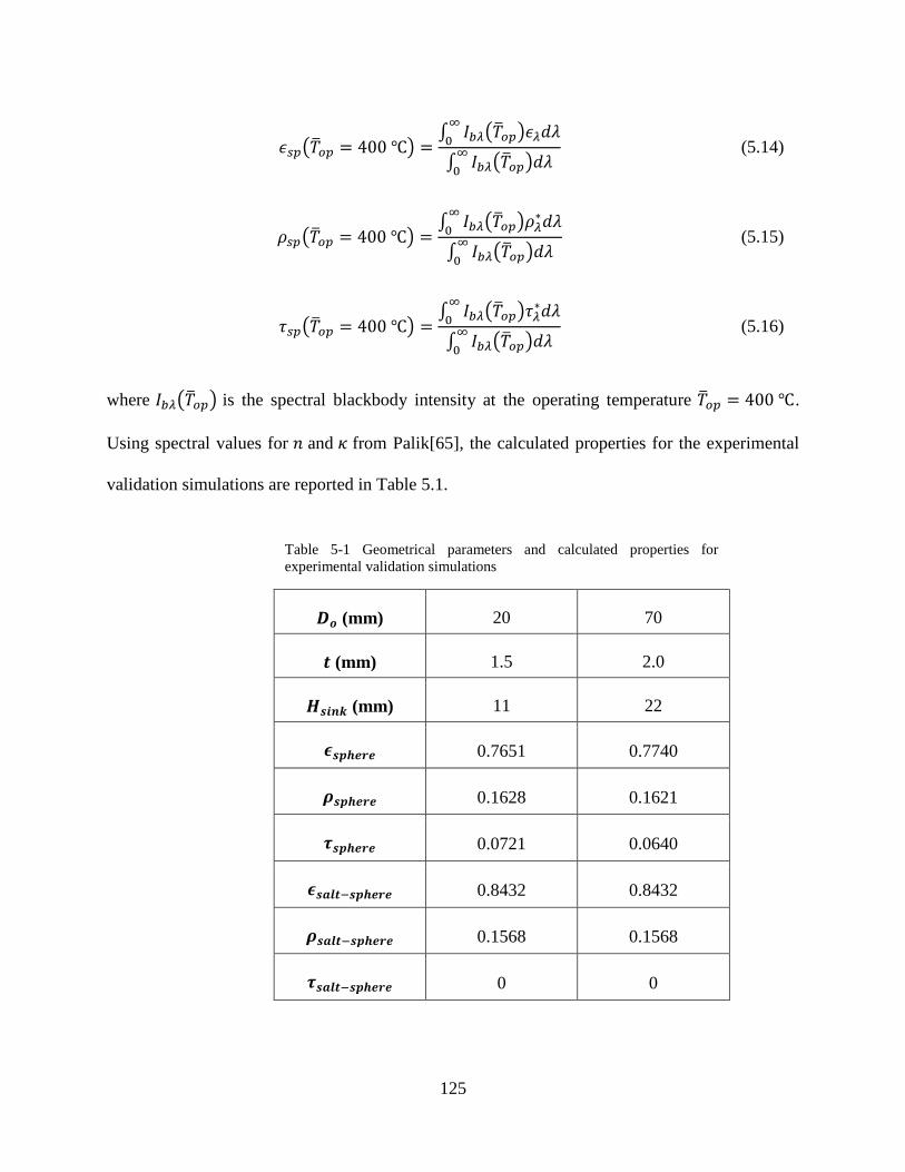
Table 5-1 Geometrical parameters and calculated properties for experimental validation

simulations .................................................................................................................................. 125

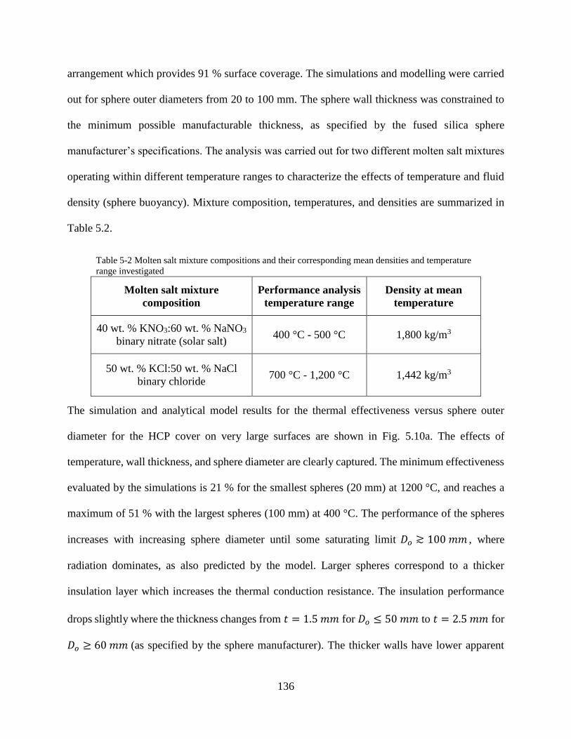
Table 5-2 Molten salt mixture compositions and their corresponding mean densities and

temperature range investigated ................................................................................................... 136

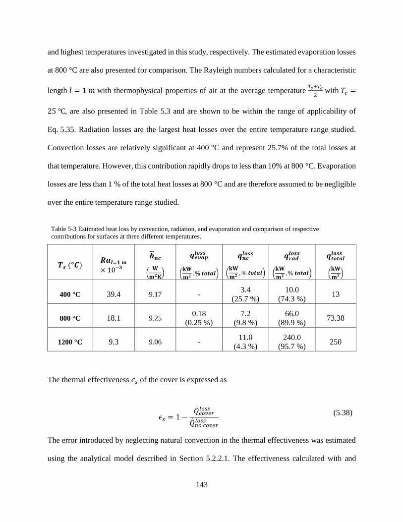
Table 5-3 Estimated heat loss by convection, radiation, and evaporation and comparison of

respective contributions for surfaces at three different temperatures. ........................................ 143

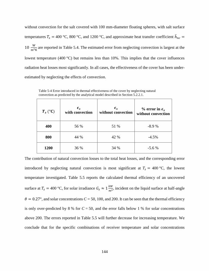
Table 5-4 Error introduced in thermal effectiveness of the cover by neglecting natural convection

as predicted by the analytical model described in Section 5.2.2.1. ............................................ 144

Table 5-5 Error introduced in calculated thermal efficiency of an uncovered receiver by neglecting

natural convection for solar irradiance 𝐺𝑠 ≈ 1𝑘𝑊/𝑚2. ............................................................. 145

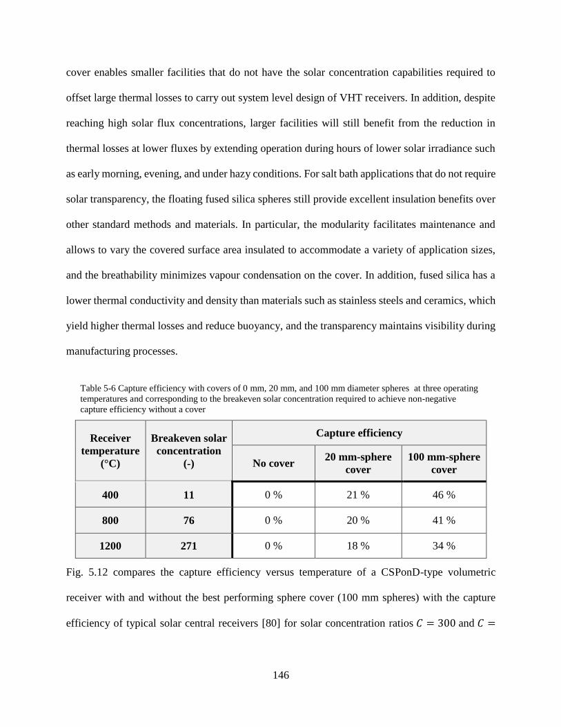
Table 5-6 Capture efficiency with covers of 0 mm, 20 mm, and 100 mm diameter spheres at three

operating temperatures and corresponding to the breakeven solar concentration required to achieve

non-negative capture efficiency without a cover ........................................................................ 146

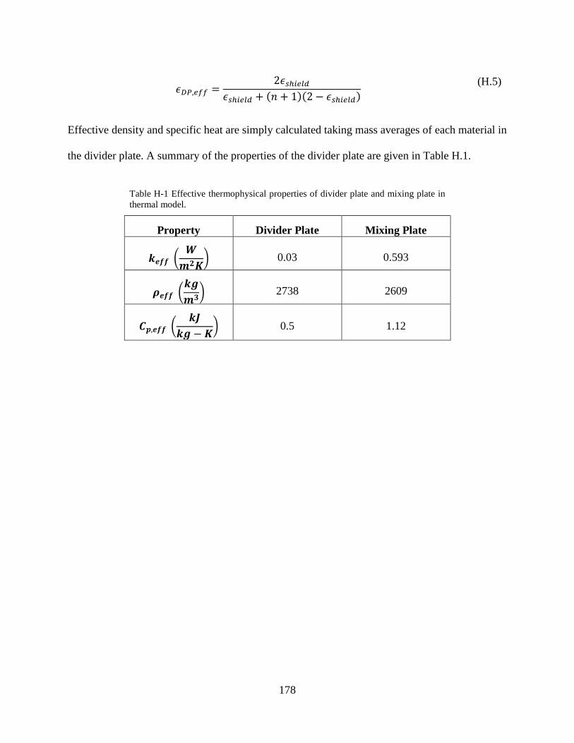
Table H-1 Effective thermophysical properties of divider plate and mixing plate in thermal model.

..................................................................................................................................................... 178

17

Nomenclature

Symbol Description Typical units

𝐴𝑚 Solar-weighted absorption factor -

𝐴𝑟𝑒𝑐 Surface area of the receiver exposed to solar irradiance m2

𝐶 Solar concentration ratio -

𝐶1 First radiation constant, W nm4 m-2

𝐶2

Second radiation constant

nm K

cp Specific heat J kg-1 K-1

𝐷𝑜 Sphere outer diameter mm

𝐹 View factor -

g Gravitational acceleration m s-2

𝐺𝑠 Solar irradiance kW m-2

ℎ𝑐𝑜𝑛𝑣 Convective heat transfer coefficient W m-2 K-1

ℎ𝑛𝑐̅̅ ̅̅ Heat transfer coefficient for natural convection W m-2 K-1

𝐻𝑠𝑖𝑛𝑘 Sink depth mm

𝐻𝑐𝑦𝑙 Cylinder length mm

Δ𝐻𝑣𝑎𝑝 Enthalpy of vaporization J/g

𝐼𝑏𝜆 Spectral blackbody intensity W m-2 μm-1

𝐼𝜆 Spectral intensity W m-2 μm-1

𝑘 Thermal conductivity W m-1 K-1

𝐿 Thickness of equivalent insulation layer mm

𝐿 Actual thickness of fluid layer m

𝐿𝑚 Average mean beam length m

𝐿𝑒,𝑆 Mean beam length through fluid thickness in solar spectrum m

𝐿𝑒,𝐸 Mean beam length through fluid thickness in re-emission spectrum m

𝑙 Characteristic length of receiver for convection m

�̇� Rate of mass transfer kg s-1

𝑛 Refractive index -

𝑁 Number of spheres -

𝑁 Conduction-to- radiation parameter -

𝑁𝑢𝑙̅̅ ̅̅ ̅ Average Nusselt number -

P Pressure Pa

Pr Prandtl number -

𝑞 Heat flux kW m-2

�̇� Rate of heat transfer kW

𝑅 Thermal resistance K W-1

R Reflectance -

𝑅𝑟𝑒𝑐 Receiver solar reflectance -

𝑅𝑎𝑙 Rayleigh number -

�̅� Average path length mm

s Geometric path length

�̇� Volumetric heat generation W m-3

t Wall thickness mm

18

t Time s

𝑇 Temperature °C

�̅�𝑜𝑝 Average operating temperature °C

𝑢𝑖 Velocity component in direction i m s-1

𝒗 velocity m s-1

∆𝑥𝑖 Fluid pathlength m

Greek letters

𝛼 Thermal diffusivity m2 s

β Coefficient of thermal expansion K-1

𝛽𝜆 Spectral attenuation coefficient m-1

𝜖 Emissivity -

𝜖𝑠 Cover thermal effectiveness -

𝜅 Absorption coefficient m-1

𝜅𝑀𝑆 Solar-weighted absorption coefficient m-1

𝜅𝑀𝐸 Re-emission-weighted absorption coefficient m-1

𝜆𝑜 Vacuum wavelength μm

𝜆 =𝜆𝑜

𝑛 Wavelength inside medium

μm

𝜈 Kinematic viscosity m2 s-1

𝜂𝑐 Capture efficiency -

𝜂𝑡ℎ Thermal efficiency -

𝜃 Irradiation half-angle °

𝛿𝑡 Themal boundary layer thickness mm

𝜌 Reflectivity -

𝜌 density kg m3

𝜌∗ Apparent reflectivity -

𝜌∥ Parallel-polarized reflectivity component -

𝜌⊥ Perpendicular-polarized reflectivity component -

𝜎 Stefan-Boltzmann constant W m-2 K-4

𝜎𝑠 Scattering coefficient m-1

𝜏 Optical thickness -

𝜏𝑀𝑆 Solar-weighted optical thickness -

𝜏𝑀𝐸 Re-emission-weighted optical thickness -

τ𝑟𝑒𝑐 Receiver transmittance -

𝜏 Transmissivity -

𝜏∗ Apparent transmissivity -

𝜇 Dynamic viscosity mPa s

𝜑 Surface coverage -

Φ𝑖 Photon flux at pixel 𝑖 m-2 s-1

Subscripts

𝑎𝑏𝑠 Absorption

𝑐𝑜𝑛𝑑 Conduction heat transfer

𝑐𝑜𝑛𝑣 Convective heat transfer

𝑒𝑓𝑓 Effective

𝑒𝑣𝑎𝑝 Evaporative losses

𝑐𝑦𝑙 Cylinder

𝑖 Pixel index

19

𝑙𝑜𝑠𝑠 Thermal loss

𝑚 Mixing layer

𝑝𝑟𝑜𝑗 Projected surface

𝑞 Quiescent

𝑟𝑎𝑑 Radiative heat transfer

𝑟𝑒𝑐 Receiver air-salt interface

𝑟𝑒𝑓 Reference situation with no cover

𝑠 Molten salt surface

𝑠𝑎𝑙𝑡 Salt surface

𝑠𝑎𝑙𝑡 − 𝑠𝑝ℎ𝑒𝑟𝑒 Salt-sphere interface

𝑠𝑝 Sphere

𝑡𝑜𝑡 Total

𝑣 Virtual surface

𝑤 Wall

∞ Environment

Abbreviations

IR Infrared

OD Outside diameter

VHT Very high temperature

20

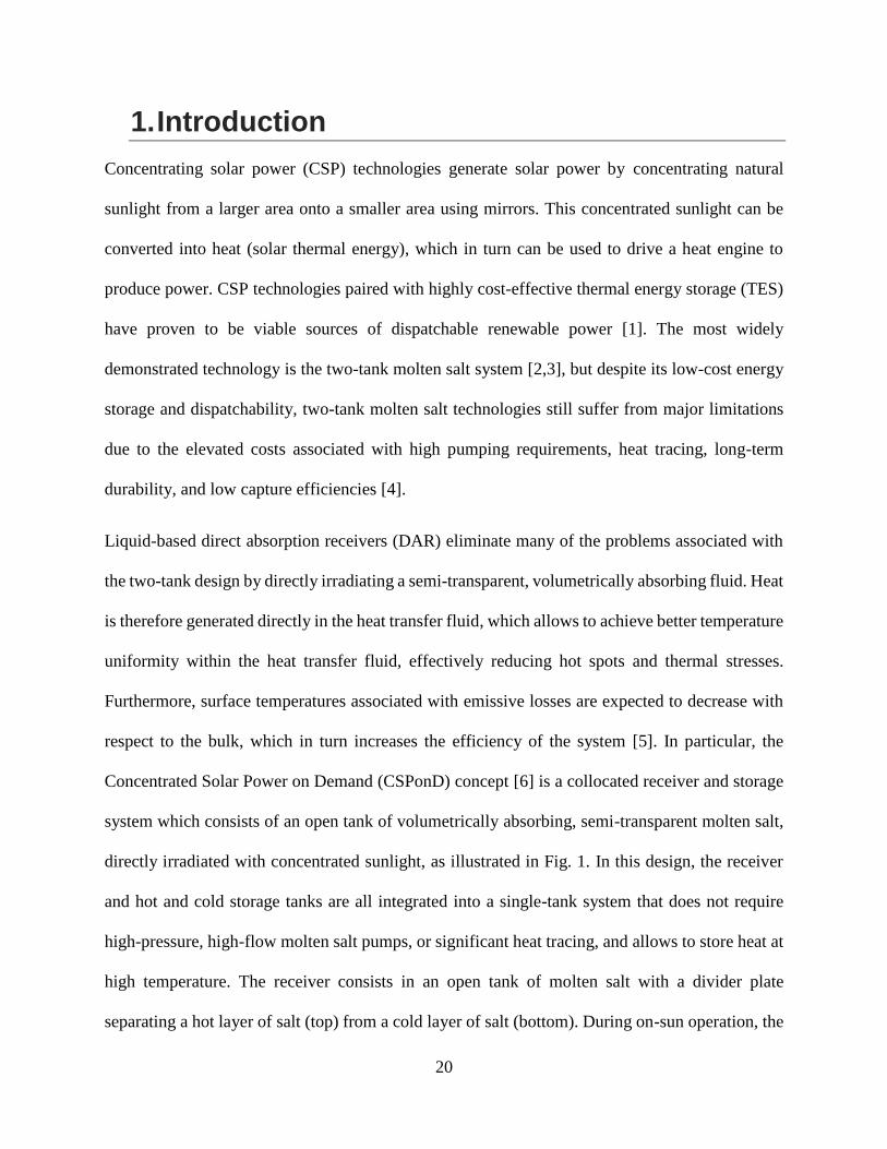
1. Introduction

Concentrating solar power (CSP) technologies generate solar power by concentrating natural

sunlight from a larger area onto a smaller area using mirrors. This concentrated sunlight can be

converted into heat (solar thermal energy), which in turn can be used to drive a heat engine to

produce power. CSP technologies paired with highly cost-effective thermal energy storage (TES)

have proven to be viable sources of dispatchable renewable power [1]. The most widely

demonstrated technology is the two-tank molten salt system [2,3], but despite its low-cost energy

storage and dispatchability, two-tank molten salt technologies still suffer from major limitations

due to the elevated costs associated with high pumping requirements, heat tracing, long-term

durability, and low capture efficiencies [4].

Liquid-based direct absorption receivers (DAR) eliminate many of the problems associated with

the two-tank design by directly irradiating a semi-transparent, volumetrically absorbing fluid. Heat

is therefore generated directly in the heat transfer fluid, which allows to achieve better temperature

uniformity within the heat transfer fluid, effectively reducing hot spots and thermal stresses.

Furthermore, surface temperatures associated with emissive losses are expected to decrease with

respect to the bulk, which in turn increases the efficiency of the system [5]. In particular, the

Concentrated Solar Power on Demand (CSPonD) concept [6] is a collocated receiver and storage

system which consists of an open tank of volumetrically absorbing, semi-transparent molten salt,

directly irradiated with concentrated sunlight, as illustrated in Fig. 1. In this design, the receiver

and hot and cold storage tanks are all integrated into a single-tank system that does not require

high-pressure, high-flow molten salt pumps, or significant heat tracing, and allows to store heat at

high temperature. The receiver consists in an open tank of molten salt with a divider plate

separating a hot layer of salt (top) from a cold layer of salt (bottom). During on-sun operation, the

21

free surface exposed to the environment is directly irradiated with sunlight as shown in Fig. 1.a. A

small fraction of incoming solar radiation is reflected at the salt surface, while the remaining

unreflected fraction penetrates the surface where it is absorbed volumetrically throughout the semi-

transparent molten salt and by the divider plate and tank walls. Actuators allow control of the

divider plate height, and an annulus between the divider plate and tank walls allows salt to move

from the cold layer to the hot layer and vice versa. During the day, the height of the divider plate

decreases to allow cold salt to flow to the hot salt layer as the hot salt layer charges. Hot salt is

continuously extracted from the top of the tank at relatively constant temperature and pumped to

a heat exchanger to extract heat for power generation. The cold (liquid) molten salt exiting the heat

exchanger is then sent back to the bottom of the tank. During night-time operation (Fig. 1.b), the

tank is closed to minimize thermal losses to the environment, and hot salt continues to be extracted

from the top layer and pumped to a heat exchanger. The divider plate height therefore increases as

the stored excess thermal energy decreases during the discharge phase.

(a) (b)

Figure 1-1 Cross-section of the general CSPonD molten salt receiver concept during (a) on-sun operation at the end

of the day, and (b) after a prolonged period with continued heat extraction but without solar heating.

22

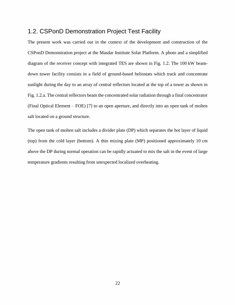
1.2. CSPonD Demonstration Project Test Facility

The present work was carried out in the context of the development and construction of the

CSPonD Demonstration project at the Masdar Institute Solar Platform. A photo and a simplified

diagram of the receiver concept with integrated TES are shown in Fig. 1.2. The 100 kW beam-

down tower facility consists in a field of ground-based heliostats which track and concentrate

sunlight during the day to an array of central reflectors located at the top of a tower as shown in

Fig. 1.2.a. The central reflectors beam the concentrated solar radiation through a final concentrator

(Final Optical Element – FOE) [7] to an open aperture, and directly into an open tank of molten

salt located on a ground structure.

The open tank of molten salt includes a divider plate (DP) which separates the hot layer of liquid

(top) from the cold layer (bottom). A thin mixing plate (MP) positioned approximately 10 cm

above the DP during normal operation can be rapidly actuated to mix the salt in the event of large

temperature gradients resulting from unexpected localized overheating.

23

(a)

(b)

Figure 1-2 (a) Photo and (b) simplified diagram of the CSPonD demonstration facility.

24

When the system is off-sun, the tank is closed with an insulating lid to reduce heat losses and to

protect the salt during inclement weather such as desert sand storms. During on-sun operation, the

incident concentrated solar radiation penetrates the salt where it is primarily absorbed

volumetrically. The remaining radiation that is not absorbed by the salt is absorbed by the tank

walls and the MP. The absorbed solar radiation is converted into heat and allows the salt

temperature to increase during the day as it stores excess thermal energy.

Design and construction of the CSPonD demonstration prototype shown in Fig. 2a was recently

completed at the Masdar Institute Solar Platform in Abu Dhabi [8,9]. The prototype has been in

operation since the completion of the construction, and the concept was successfully demonstrated

experimentally by thermally cycling molten salt between 280 °C and 450 °C during daily

charging/discharging cycles. Nevertheless, the molten salt receiver is subjected to volumetric

heating conditions that produce complex thermal and flow behavior within the salt that remain

poorly understood [10] and limits the ability to make accurate thermal-hydraulics predictions. The

desired temperature profile within the hot salt layer could not be predicted and was therefore

maintained using feedback controls for the divider plate motion. Improving our understanding of

complex heating and flow conditions in direct absorption, liquid-based volumetric receivers is

therefore necessary to further improve the design and operation of this technology which remains

in its early stages of development.

1.3. Participating media and natural convection in internally heated fluids

The interaction of a material with thermal radiation depends on its optical properties. For semi-

transparent liquids such as molten salts, thermal radiation emitted within the fluid itself or from an

external source travels an appreciable distance within the fluid between interactions. Such media

25

are known as participating media. Their interaction with thermal radiation is in contrast with

transparent media which involve only surface interactions at the boundaries, known as surface-to-

surface radiation. The radiation transport in participating media is governed by the radiative

transfer equation, given as

𝑑𝐼𝜆

𝑑𝑠= 𝜅𝜆𝐼𝑏𝜆 − 𝛽𝜆𝐼𝜆 +

𝜎𝑠𝜆

4𝜋∫ 𝐼𝜆(�̂�𝑖)Φ𝜆(�̂�𝑖

4𝜋

, �̂�)𝑑Ω𝑖 (1.1)

where 𝜅𝜆 is the spectral absorption coefficient, 𝜎𝑠𝜆 is the spectral scattering coefficient, 𝛽𝜆 = 𝜅𝜆 +

𝜎𝑠𝜆 is the spectral attenuation coefficient and is expressed as the sum of the absorption and

scattering coefficients, 𝛺 is the solid angle, 𝜆 is the wavelength, 𝐼𝑏𝜆 is the spectral blackbody

radiative intensity, 𝐼𝜆 is the radiative intensity, and 𝑠 is the path. For non-scattering liquids (𝜎𝑠𝜆 ≈

0), the radiative transfer equation reduces to

𝑑𝐼𝜆

𝑑𝑠≈ 𝜅𝜆(𝐼𝑏𝜆 − 𝐼𝜆) (1.2)

When an external source of radiation such as the sun is incident upon a participating media’s

boundary, this radiation will penetrate and be absorbed within the volume of the medium, resulting

in volumetric heat generation. This volumetric heat generation is described by the radiative flux

equation, given as

𝛻 ∙ 𝒒𝑹 = ∫ 𝜅𝜆 (4𝜋𝐼𝑏𝜆 − ∫ 𝐼𝜆𝑑𝛺4𝜋

)∞

𝜆=0

𝑑𝜆 (1.3)

26

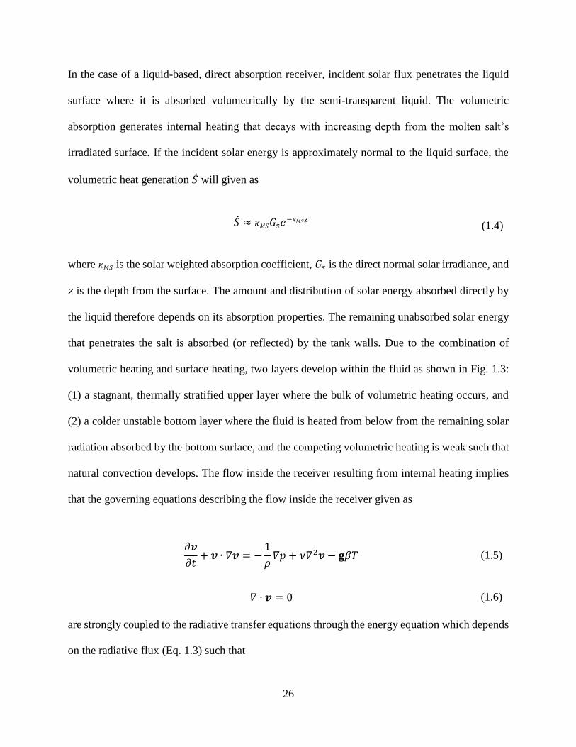
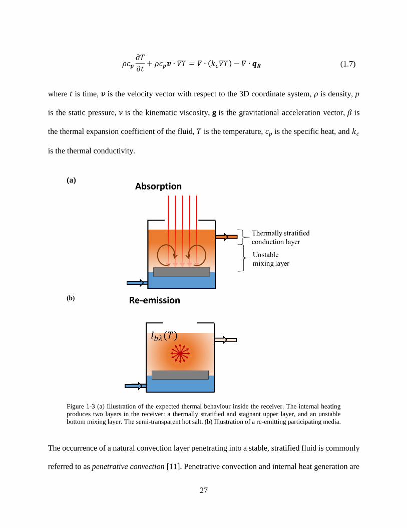
In the case of a liquid-based, direct absorption receiver, incident solar flux penetrates the liquid

surface where it is absorbed volumetrically by the semi-transparent liquid. The volumetric

absorption generates internal heating that decays with increasing depth from the molten salt’s

irradiated surface. If the incident solar energy is approximately normal to the liquid surface, the

volumetric heat generation �̇� will given as

�̇� ≈ 𝜅𝑀𝑆𝐺𝑠𝑒−𝜅𝑀𝑆𝑧 (1.4)

where 𝜅𝑀𝑆 is the solar weighted absorption coefficient, 𝐺𝑠 is the direct normal solar irradiance, and

𝑧 is the depth from the surface. The amount and distribution of solar energy absorbed directly by

the liquid therefore depends on its absorption properties. The remaining unabsorbed solar energy

that penetrates the salt is absorbed (or reflected) by the tank walls. Due to the combination of

volumetric heating and surface heating, two layers develop within the fluid as shown in Fig. 1.3:

(1) a stagnant, thermally stratified upper layer where the bulk of volumetric heating occurs, and

(2) a colder unstable bottom layer where the fluid is heated from below from the remaining solar

radiation absorbed by the bottom surface, and the competing volumetric heating is weak such that

natural convection develops. The flow inside the receiver resulting from internal heating implies

that the governing equations describing the flow inside the receiver given as

𝜕𝒗

𝜕𝑡+ 𝒗 ∙ 𝛻𝒗 = −

1

𝜌𝛻𝑝 + 𝜈𝛻2𝒗 − 𝐠𝛽𝑇 (1.5)

𝛻 ∙ 𝒗 = 0 (1.6)

are strongly coupled to the radiative transfer equations through the energy equation which depends

on the radiative flux (Eq. 1.3) such that

27

𝜌𝑐𝑝

𝜕𝑇

𝜕𝑡+ 𝜌𝑐𝑝𝒗 ∙ 𝛻𝑇 = 𝛻 ∙ (𝑘𝑐𝛻𝑇) − 𝛻 ∙ 𝒒𝑹 (1.7)

where 𝑡 is time, 𝒗 is the velocity vector with respect to the 3D coordinate system, 𝜌 is density, 𝑝

is the static pressure, 𝜈 is the kinematic viscosity, 𝐠 is the gravitational acceleration vector, 𝛽 is

the thermal expansion coefficient of the fluid, 𝑇 is the temperature, 𝑐𝑝 is the specific heat, and 𝑘𝑐

is the thermal conductivity.

(a)

(b)

Figure 1-3 (a) Illustration of the expected thermal behaviour inside the receiver. The internal heating

produces two layers in the receiver: a thermally stratified and stagnant upper layer, and an unstable

bottom mixing layer. The semi-transparent hot salt. (b) Illustration of a re-emitting participating media.

The occurrence of a natural convection layer penetrating into a stable, stratified fluid is commonly

referred to as penetrative convection [11]. Penetrative convection and internal heat generation are

28

present in a wide variety of geophysical and astrophysical phenomena such as convection resulting

from solar heating in the atmosphere, oceans, lakes and reservoirs [11,12], stellar convection [13],

and volumetrically absorbing solar receivers. Convection generated by internal heating is also an

important heat transfer process in several nuclear reactor applications such as heat generation in

spent nuclear pools and during post-accident heat removal [14–16].

Previous analyses of the thermal-fluid behavior of liquid filled cavities with solar radiation

absorption have typically been limited to 2D numerical studies of isolated cavities [17–19], and in

some cases neglect the effects of convection entirely [20]. In addition, studies of radiation induced

convection are typically concerned with low temperature applications such as absorption in water

bodies, and do not allow for the possibility of internal re-radiation. In particular, Hattori et al. [21]

developed an analytical solution for the nonlinear temperature stratification and its effects on

internal mixing for water bodies subjected to heating by solar radiation. The two-dimensional

analysis was carried out for a simple adiabatic surface boundary condition and was validated

numerically. None of the previous investigations model a solar receiver under real operating

conditions and limited analytical and computational tools exist for making predictions for better

design and optimization. Furthermore, analyses have been limited to low temperature water

applications and do not account for the significant effects of radiative cooling at the surface. The

fundamental numerical and scaling analyses provide insufficient insight into complex behavior of

the system and the design and operation of a receiver.

1.4. Molten Salts

Typical solar collectors absorb incident solar radiation through surface absorbers before

transferring this radiation as thermal energy to a working fluid or storage material. The CSPonD

29

concept uses a volumetrically absorbing high temperature fluid as storage medium and working

fluid as an alternative solar absorption approach which allows incident solar radiation to be directly

absorbed and stored by the working fluid and eliminates the need for intermediate surface

absorbers. This alternative absorption and storage method allows to increase performance and

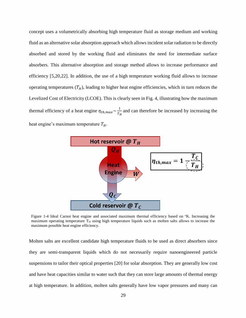
efficiency [5,20,22]. In addition, the use of a high temperature working fluid allows to increase

operating temperatures (𝑇𝐻), leading to higher heat engine efficiencies, which in turn reduces the

Levelized Cost of Electricity (LCOE). This is clearly seen in Fig. 4, illustrating how the maximum

thermal efficiency of a heat engine 𝜂𝑡ℎ,𝑚𝑎𝑥~1

𝑇𝐻 and can therefore be increased by increasing the

heat engine’s maximum temperature 𝑇𝐻.

Figure 1-4 Ideal Carnot heat engine and associated maximum thermal efficiency based on oK. Increasing the

maximum operating temperature TH using high temperature liquids such as molten salts allows to increase the

maximum possible heat engine efficiency.

Molten salts are excellent candidate high temperature fluids to be used as direct absorbers since

they are semi-transparent liquids which do not necessarily require nanoengineered particle

suspensions to tailor their optical properties [20] for solar absorption. They are generally low cost

and have heat capacities similar to water such that they can store large amounts of thermal energy

at high temperature. In addition, molten salts generally have low vapor pressures and many can

30

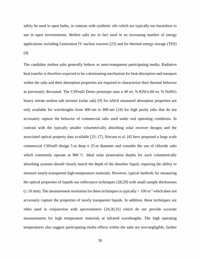
safely be used in open baths, in contrast with synthetic oils which are typically too hazardous to

use in open environments. Molten salts are in fact used in an increasing number of energy

applications including Generation IV nuclear reactors [23] and for thermal energy storage (TES)

[4].

The candidate molten salts generally behave as semi-transparent participating media. Radiative

heat transfer is therefore expected to be a dominating mechanism for heat absorption and transport

within the salts and their absorption properties are required to characterize their thermal behavior

as previously discussed. The CSPonD Demo prototype uses a 40 wt. % KNO3:60 wt. % NaNO3

binary nitrate molten salt mixture (solar salt) [9] for which measured absorption properties are

only available for wavelengths from 400 nm to 800 nm [24] for high purity salts that do not

accurately capture the behavior of commercial salts used under real operating conditions. In

contrast with the typically smaller volumetrically absorbing solar receiver designs and the

associated optical property data available [25–27], Slocum et al. [6] have proposed a large scale

commercial CSPonD design 5 m deep × 25 m diameter and consider the use of chloride salts

which commonly operate at 900 ˚C. Ideal solar penetration depths for such volumetrically

absorbing systems should closely match the depth of the absorber liquid, requiring the ability to

measure nearly-transparent high-temperature materials. However, typical methods for measuring

the optical properties of liquids use reflectance techniques [28,29] with small sample thicknesses

(≤ 10 mm). The measurement resolution for these techniques is typically > 100 m-1 which does not

accurately capture the properties of nearly transparent liquids. In addition, these techniques are

often used in conjunction with spectrometers [24,30,31] which do not provide accurate

measurements for high temperature materials at infrared wavelengths. The high operating

temperatures also suggest participating media effects within the salts are non-negligible, further

31

emphasizing the necessity of measuring optical properties over a wider spectral range extending

into the mid-infrared spectrum. It is therefore of great value to characterize the solar absorption,

the internal re-emission, and the radiative losses for these systems at elevated temperatures.

1.5. Thermal losses in open tanks of molten salt

The benefits of operating solar-receivers at higher temperatures are often offset by significant

thermal losses, particularly for relatively low solar concentration ratios 𝐶 [32] in an open-tank

configuration. This can be understood in terms of the receiver thermal efficiency 𝜂𝑡ℎ, defined as

the ratio of collected thermal energy to total incident solar energy [20], which is given by

𝜂𝑡ℎ =�̇�𝑎𝑏𝑠 − �̇�𝑙𝑜𝑠𝑠

𝐶𝐺𝑠𝐴𝑟𝑒𝑐 (1.8)

where �̇�𝑎𝑏𝑠 is the solar power absorbed by the receiver, 𝐶 is the solar concentration ratio, 𝐺𝑠 is

the direct normal irradiance, 𝐴𝑟𝑒𝑐 is the surface area of the receiver exposed to the concentrated

solar irradiation, and �̇�𝑙𝑜𝑠𝑠 is the sum of the convective, conductive, evaporative, and radiative

heat losses to the environment. For a sufficiently deep receiver with highly absorbing containment

walls, most of the non-reflected incident energy is absorbed such that �̇�𝑎𝑏𝑠 ≈ (1 − 𝑅𝑟𝑒𝑐)𝐶𝐺𝑠𝐴𝑟𝑒𝑐,

where 𝑅𝑟𝑒𝑐 is the receiver’s solar reflectance, and the thermal efficiency becomes

𝜂𝑡ℎ ≈ (1 − 𝑅𝑟𝑒𝑐) −�̇�𝑐𝑜𝑛𝑣

𝑙𝑜𝑠𝑠 + �̇�𝑒𝑣𝑎𝑝𝑙𝑜𝑠𝑠 + �̇�𝑟𝑎𝑑

𝑙𝑜𝑠𝑠


For moderate to low solar concentration ratios, thermal losses, and in particular radiative losses

�̇�𝑟𝑎𝑑𝑙𝑜𝑠𝑠 at high temperature, will be significant relative to the total incident concentrated solar energy

𝐶𝐺𝑠𝐴𝑟𝑒𝑐, resulting in low thermal efficiencies.

32

In addition to impeding the capture efficiency of a receiver, the large thermal losses at the liquid

surface also lead to very large thermal gradients near the salt surface as illustrated in Fig. 3. The

temperature at the surface will typically be significantly reduced due to radiative cooling, and the

temperature rapidly increases in only a few centimeters immediately below the liquid surface

where the volumetric heating is strongest.

Many methods have been explored to mitigate these losses in a wide variety of solar-thermal

applications [33–39]. In particular, spectrally selective surface absorbers are engineered to

maximize solar absorptivity and minimize thermal radiative losses [40–42]. High temperature

open-top liquid-based receivers such as the CSPonD have large radiative and convective losses

that are much more challenging to manage. Standard methods for reducing losses such as reflective

cavities [33,34] and windows [36,39] cannot readily be implemented in open-tank configurations,

and their effectiveness is limited due to fabrication, cost, and operation constraints especially in a

desert environment [43,44].

1.6. Objectives

In order for liquid-based direct absorption volumetric solar receivers to become competitive CSP

energy technologies, the efficiency and operation must be improved in order to reduce capital and

operation costs. The complex nature of internally heated fluids and the unique open-tank design at

high temperature are major challenges in optimizing the design and operation in volumetrically

absorbing solar receiver. A complete thermal-hydraulics analysis will therefore provide significant

insight into the complex thermal-fluid behavior of the receiver, allowing to identify optimal

operating conditions and to prevent critical system failures due to thermal stresses and thermal

degradation resulting from large temperature non-uniformities.

33

1.6.1. Scope of thesis

Given the importance in solar receiver design and the limited studies available for predicting the

thermal behavior in volumetrically absorbing solar receivers, this thesis focuses on characterizing

and improving the thermal-hydraulic design and operation of a CSPonD receiver. In addition, the

design of a transparent cover created from hollow quartz spheres is presented as a means to reduce

thermal losses. This work was carried out in collaboration with researchers in the Nuclear and

Mechanical Engineering departments at MIT, and with Prof. Nicolas Calvet’s research group at

the Masdar Institute Solar Platform in Abu Dhabi. The broader scope of the project was the

development and construction of the CSPonD Demonstration Project at the Masdar Institute Solar

Platform which was completed and went into operation in June 2017.

The thesis focuses on four main aspects as illustrated in Fig. 1.5: (1) fundamental molten salt

properties, (2) theoretical analysis, (3) computational modeling, and (4) thermal design

improvements. Chapter 2 describes the experimental apparatus developed and used for measuring

the optical properties of nearly-transparent, high temperature liquids, and presents the

measurement results. Chapter 3 outlines the fundamental thermal-fluid scaling parameters in the

receiver and presents theoretical analysis of the optimal operation and design conditions. Chapter

4 presents the computational fluid dynamics (CFD) and heat transfer model of the entire receiver

using the measured optical properties presented in Chapter 2, and compares the results with

experimental results collected at the CSPonD Demonstration Project test facility. Chapter 5 details

the design of a solar-transparent, modular molten salt cover for insulating the open tank receiver

to improve the thermal efficiency and increase the temperature uniformity. Finally, Chapter 6

summarizes the critical take-aways from the presented work and outlines future research paths.

34

Figure 1-5 Illustration summarizing the four principal thermal-fluid topics investigated in this thesis.

35

2. Molten salt optical properties measurements

In this section, we present a simple and accurate apparatus that allows for the precise measurement

of light attenuation in high temperature, nearly transparent liquids, over a broad spectrum

extending from the visible region (400 nm) into mid-infrared (8 µm). The apparatus is used to

measure the attenuation of light in the 40 wt. % KNO3:60 wt. % NaNO3 binary nitrate and the

50 wt. % KCl:50 wt. % NaCl binary chloride molten salt mixtures. The effects of salt

contamination due to thermal decomposition are also evaluated. Sources of contamination in the

CSPonD include thermal decomposition due to unexpected heating conditions and local hot spots,

and sand/dust contamination due to the open receiver design. The implications of the results are

discussed in the context of the CSPonD Demo and for general volumetrically absorbing solar

receiver applications.

2.1. Experimental Procedure

2.1.1. Apparatus description

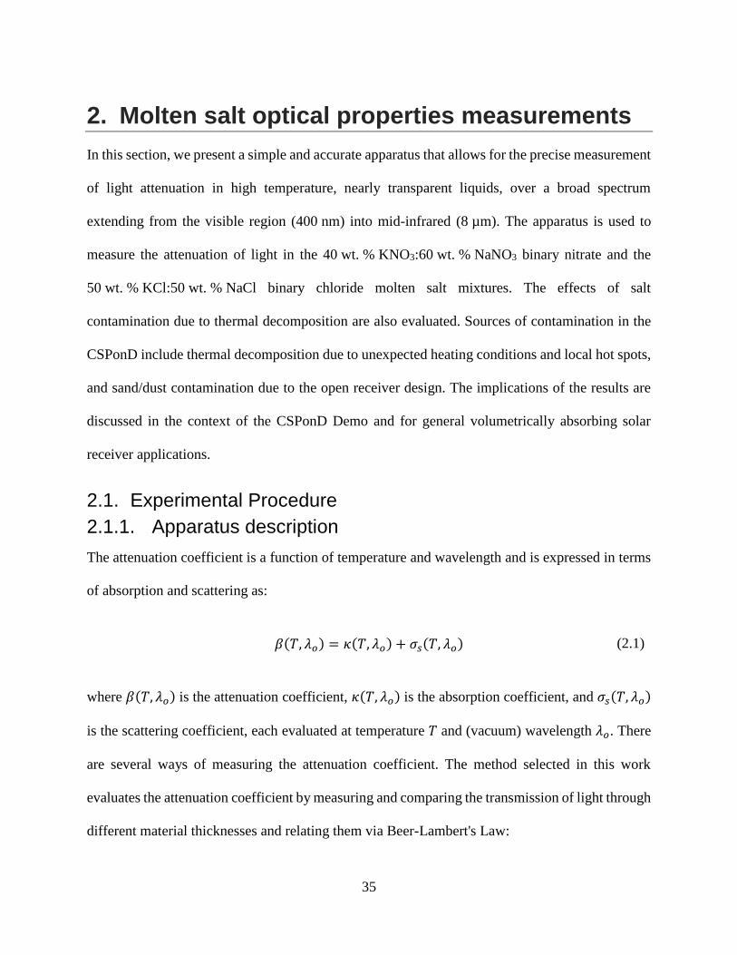
The attenuation coefficient is a function of temperature and wavelength and is expressed in terms

of absorption and scattering as:

𝛽(𝑇, 𝜆𝑜) = 𝜅(𝑇, 𝜆𝑜) + 𝜎𝑠(𝑇, 𝜆𝑜) (2.1)

where 𝛽(𝑇, 𝜆𝑜) is the attenuation coefficient, 𝜅(𝑇, 𝜆𝑜) is the absorption coefficient, and 𝜎𝑠(𝑇, 𝜆𝑜)

is the scattering coefficient, each evaluated at temperature 𝑇 and (vacuum) wavelength 𝜆𝑜. There

are several ways of measuring the attenuation coefficient. The method selected in this work

evaluates the attenuation coefficient by measuring and comparing the transmission of light through

different material thicknesses and relating them via Beer-Lambert's Law:

36

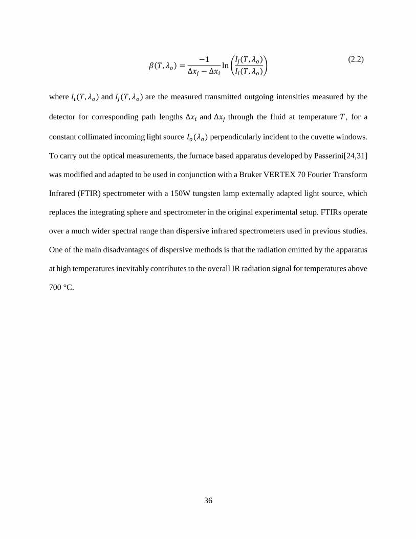
𝛽(𝑇, 𝜆𝑜) =

−1

∆𝑥𝑗 − ∆𝑥𝑖ln (

𝐼𝑗(𝑇, 𝜆𝑜)

𝐼𝑖(𝑇, 𝜆𝑜))

(2.2)

where 𝐼𝑖(𝑇, 𝜆𝑜) and 𝐼𝑗(𝑇, 𝜆𝑜) are the measured transmitted outgoing intensities measured by the

detector for corresponding path lengths ∆𝑥𝑖 and ∆𝑥𝑗 through the fluid at temperature 𝑇 , for a

constant collimated incoming light source 𝐼𝑜(𝜆𝑜) perpendicularly incident to the cuvette windows.

To carry out the optical measurements, the furnace based apparatus developed by Passerini[24,31]

was modified and adapted to be used in conjunction with a Bruker VERTEX 70 Fourier Transform

Infrared (FTIR) spectrometer with a 150W tungsten lamp externally adapted light source, which

replaces the integrating sphere and spectrometer in the original experimental setup. FTIRs operate

over a much wider spectral range than dispersive infrared spectrometers used in previous studies.

One of the main disadvantages of dispersive methods is that the radiation emitted by the apparatus

at high temperatures inevitably contributes to the overall IR radiation signal for temperatures above

700 °C.

37

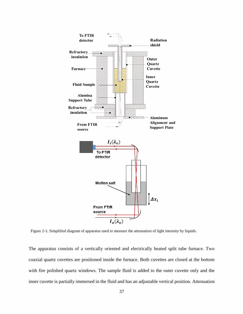
Figure 2-1. Simplified diagram of apparatus used to measure the attenuation of light intensity by liquids.

The apparatus consists of a vertically oriented and electrically heated split tube furnace. Two

coaxial quartz cuvettes are positioned inside the furnace. Both cuvettes are closed at the bottom

with fire polished quartz windows. The sample fluid is added to the outer cuvette only and the

inner cuvette is partially immersed in the fluid and has an adjustable vertical position. Attenuation

38

measurements can therefore easily be made for different fluid thicknesses by adjusting the inner

cuvette’s height. Heights of up to 10 cm provide the sensitivity required to measure the nearly

transparent salt’s attenuation coefficient. The double cuvette design is also advantageous because

it minimizes vibrational issues by eliminating the free surface of the fluid from the beam path. A

schematic of the apparatus is shown in Fig. 2.1 and a picture of the apparatus is presented in

Fig. 2.2.

As illustrated in the diagram, the outgoing intensities are measured by the FTIR detector for

different path lengths through the liquid. The selected double cuvette design and method for

calculating attenuation coefficient eliminate the effects of surface reflections at the cuvette

interfaces and any effects from impurities deposited at the bottom of the cuvette. Impurity deposits

correspond to a constant attenuation over all path lengths and do not contribute to the volumetric

attenuation. A radiation shield was required for the much higher temperature chloride in order to

prevent undesirable photons emitted by the hot fluid surface from saturating the detector. The

radiation shield is made of refractory material wrapped in aluminum foil with a small aperture in

the center allowing the light source to pass through. The design can also be extended to

wavelengths between 2.5 µm and 5.0 µm where quartz is only partially transmissive since its

attenuation is constant at all path lengths. For measurements at wavelengths greater than 5.0 µm,

the quartz windows would be replaced with a more optically transmissive window material such

as diamond, zinc selenide, or calcium fluoride. Window material selection will also depend on its

compatibility with the measured fluid.

39

Figure 2-2 Picture of the experimental apparatus for measuring the attenuation of light of high temperature liquids.

2.1.2. Mixture preparation

Refined grade sodium and potassium nitrate salts (>99.5 % purity) were provided by SQM and

pre-mixed to obtain a 40 wt. % KNO3:60 wt. % NaNO3 binary nitrate molten salt mixture. Sodium

and potassium chloride salts (>99.0% purity) were purchased separately from Alfa Aesar

(https://www.alfa.com/en/ product numbers #12314 and #11595) and pre-mixed to obtain a

50 wt. % KCl:50 wt. % NaCl binary chloride molten salt mixture. None of the salts contained anti-

caking agents.

The salts are then dried in an oven at 50 ˚C for at least 1 hour to remove excess moisture before

being loaded in the outer cuvette. A K-type thermocouple positioned at the mid-height of the

40

furnace on the outer wall of the outer cuvette is connected to a temperature controller, which

controls the furnace output and allows the salts to be heated at a slow and steady rate to a set

temperature. Passerini and McKrell[31] characterized the axial variation in temperature along the

outer cuvette and reported a maximum deviation of 10%.

Thermal decomposition of the binary nitrate molten salt mixture was achieved by raising the

temperature of the molten salt to 550 ˚C (open system decomposition temperature[45]) for

45 minutes. Bubbling was observed during decomposition and the salt developed a green tint. The

results for the three salts investigated are shown in Fig. 2.3. in their molten state.

(a) (b) (c)

Figure 2-3 40 wt. % KNO3:60 wt. % NaNO3 binary nitrate molten salt mixture at 400 ˚C (a), decomposed binary

nitrate molten salt mixture at 400 ˚C (b), and 50 wt. % KCl:50 wt. % NaCl binary chloride molten salt mixture at

400 ˚C (c).

41

2.1.3. Measurement procedure

Once the salt mixture has melted, the inner cuvette is moved to its lowest position corresponding

to approximately 1-2 cm of liquid thickness, and a transmission spectrum is acquired at each

vertical position in 5 mm increments up to its highest position. Once the maximum position is

reached, the cuvette is lowered and the measurements are taken again in 5 mm downward

increments to ensure repeatability of the collected data versus depth. In total, measurements were

taken twice for 10 to 20 different path lengths. In addition, the measurements were acquired for

three different salt temperatures for the nitrate mixture: 300 ˚C, 350 ˚C, and 400 ˚C, and at 800 ˚C

for the chloride mixture due to its weak temperature dependence as will be discussed. The

transmission spectrum scanning resolution is 8 cm-1 (< 5 nm resolution over the measured

spectrum). Error bars are only given every 25 nm for clarity. In addition, a moving average filter

with a maximum size of 160 cm-1 (< 20 nm) was used in the visible spectrum to compensate for

the noise in the signal.

2.2.3. Thermal performance evaluation

To understand the thermal behavior of the salt and in particular the radiative heat transfer within

the different media, we consider three factors: the general participating media behavior, the

volumetric absorption, and the effective emissivity. The latter two can be considered together in

the capture efficiency. We first define solar-weighted and re-emission-weighted absorption

coefficients and optical thicknesses for the fluids, given as

𝜅𝑀𝑆 =

∫ 𝐺𝑠𝜅𝜆𝑜𝑑𝜆𝑜

∞

0

∫ 𝐺𝑠𝑑𝜆𝑜∞

0

, (2.3)

42

𝜅𝑀𝐸 =

∫ 𝐼𝑏𝜆𝑜(�̅�𝑜𝑝)𝜅𝜆𝑜

𝑑𝜆𝑜∞

0

∫ 𝐼𝑏𝜆𝑜(�̅�𝑜𝑝)𝑑𝜆𝑜

∞

0

, (2.4)

𝜏𝑀𝑆 = 𝜅𝑀𝑆𝐿𝑒,𝑆 and 𝜏𝑀𝐸 = 𝜅𝑀𝐸𝐿𝑒,𝐸 (2.5)

where 𝐺𝑠 is the spectral solar irradiance[46], 𝜅𝜆𝑜 is the measured spectral absorption coefficient of

the fluid, 𝐿𝑒,𝑆 and 𝐿𝑒,𝐸 are the mean beam lengths through the fluid thickness, and 𝐼𝑏𝜆𝑜(�̅�𝑜𝑝) is the

spectral emissive blackbody intensity inside the fluid at its average operating temperature �̅�𝑜𝑝,

given by Planck’s Law:

𝐼𝑏𝜆(�̅�𝑜𝑝) =

𝐶1

𝜋𝑛2𝜆5[𝑒 𝐶2 (𝑛𝜆�̅�𝑜𝑝)⁄ − 1]

(2.6)

where 𝐶1 and 𝐶2 are the first and second radiation constants, 𝑛 is the index of refraction of the

fluid, and 𝜆 are wavelengths inside the medium, defined as 𝜆 =𝜆𝑜

𝑛. In the optically thick limit

where 𝜏 → ∞, the medium behaves as an opaque body with negligible participating media effects,

and the heat flux at the surface approaches the same value as for a blackbody radiator[47,48]. In

the limit where 𝜏 ≪ 1, the medium is said to be optically thin and its re-emitted radiation travels

long distances without being absorbed by itself. In this work, we assume scattering to be

negligible[26] and take the absorption coefficient to be approximately equal to the measured

attenuation coefficient.

The solar absorption performance can be characterized by evaluating the solar-weighted

absorption factor. The value yields the percentage of incoming solar energy absorbed by the

medium for a given thickness[25] and is defined as:

43

𝐴𝑚 =

(1 − 𝑅) ∫ 𝐺𝑠(1 − 𝑒−𝜅𝜆𝑜𝐿𝑒,𝑆)𝑑𝜆𝑜∞

0


0

(2.7)

where 𝑅 is the reflectance at the surface. The radiative losses to the environment are characterized

by the total emissivity of an isothermal fluid layer of thickness 𝐿𝑒,𝐸 given as

𝜖(𝐿𝑒,𝐸 , �̅�𝑜𝑝) = (

∫ 𝐼𝑏𝜆𝑜(�̅�𝑜𝑝)(1 − 𝑒−𝜅𝜆𝑜𝐿𝑒,𝐸)𝑑𝜆𝑜

∞

0

∫ 𝐼𝑏𝜆𝑜(�̅�𝑜𝑝)𝑑𝜆𝑜

∞

0

) (2.8)

Finally, we evaluate the capture efficiency of the medium as

𝜂𝑐 =

(1 − 𝑅) ∫ 𝐺𝑠(1 − 𝑒−𝜅𝜆𝑜𝐿𝑒,𝑆)𝑑𝜆𝑜∞

0


0

−𝑞𝑠

𝐶 ∫ 𝐺𝑠𝑑𝜆𝑜∞

0

= 𝐴𝑚 −𝑞𝑠

𝐶 ∫ 𝐺𝑠𝑑𝜆𝑜∞

0

(2.9)

where 𝐶 is the solar concentration factor. 𝑞𝑠 is the heat flux at the surface of the isothermal

medium, assuming a vacuum boundary condition at the surface, and is defined as

𝑞𝑠 = 𝜖(𝐿𝑒,𝐸 , �̅�𝑜𝑝)𝑛2𝜎�̅�𝑜𝑝4 (2.10)

where 𝑛 is the refractive index of the medium and 𝜎 is the Stefan-Boltzmann constant.

In this work, we take the average operating temperature as 400 ˚C for the binary nitrate and 800 ˚C

for the binary chloride. From the Kramers-Krönig dispersion relations[47,49–51], the refractive

index has wavelength dependence related to the absorption properties, with only small variations

away from the absorption peaks. The chloride-based salts are therefore not expected to show large

variation in n below 14 µm. Furthermore, experimental evidence from Makino[52] confirms

negligible n-variation in the nitrate salts for wavelengths below 5 µm. Therefore, the refractive

indices are simply taken to be the published values measured at the 589 nm sodium D line, where

44

n=1.41 for eutectic NaNO3-KNO3[53] and n=1.40 for the mass weighted average properties of the

50 wt. % KCl (n=1.417):50 wt. % NaCl (n=1.385)[54,55].

In order to characterize the performance of the salt itself, independently of the containment vessel

wall’s properties, we assume the fluids are contained in infinite slabs with fully reflective bottom

boundary and fully transmissive top boundary, and solar irradiance normal to the surface of the

fluid, as illustrated in Fig. 2.4 The mean beam lengths through the fluid are therefore 𝐿𝑒,𝑆 = 2𝐿

for the solar absorption, where 𝐿 is the actual thickness of the fluid, and 𝐿𝑒,𝐸 = 2𝐿𝑚 for the re-

emission, where 𝐿𝑚 is the average mean beam length given by Modest[47] as 𝐿𝑚 = 1.76𝐿 for an

infinite slab.

Figure 2-4 Diagram illustrating assumptions and boundary conditions for performance evaluation.

45

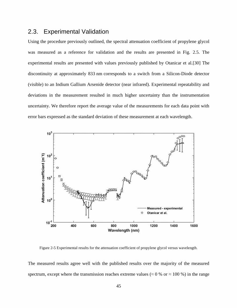
2.3. Experimental Validation

Using the procedure previously outlined, the spectral attenuation coefficient of propylene glycol

was measured as a reference for validation and the results are presented in Fig. 2.5. The

experimental results are presented with values previously published by Otanicar et al.[30] The

discontinuity at approximately 833 nm corresponds to a switch from a Silicon-Diode detector

(visible) to an Indium Gallium Arsenide detector (near infrared). Experimental repeatability and

deviations in the measurement resulted in much higher uncertainty than the instrumentation

uncertainty. We therefore report the average value of the measurements for each data point with

error bars expressed as the standard deviation of these measurement at each wavelength.

Figure 2-5 Experimental results for the attenuation coefficient of propylene glycol versus wavelength.

The measured results agree well with the published results over the majority of the measured

spectrum, except where the transmission reaches extreme values (≈ 0 % or ≈ 100 %) in the range

46

of thicknesses measured. The uncertainty is largest and diverges most from the published results

between 500 nm and 600 nm where the attenuation is on the order of 1 m-1. Nevertheless,

uncertainty due to repeatability in the measurements remains below 20 % at all reported

wavelengths. The maximum deviation between the measured and published average values is also

at this location, where the two deviate 40 %. Below 425 nm, the intensity of the light source decays

too rapidly to obtain accurate measurements. Above 1400 nm, the attenuation approaches 103 m-1

such that the transmission becomes too small to detect for the sensitivity of the apparatus. Given

these results, the optimal accuracy is achieved for wavelengths above 425 nm and for attenuation

coefficients between 0.5 m-1 to 500 m-1.

2.4. Results

Figure 2-6 Attenuation Coefficient of 40 wt. % KNO3: 60 wt. % NaNO3 binary nitrate molten salt (SQM) at 400

˚C.

47

Figure 2-7 Attenuation Coefficient of decomposed 40 wt. % KNO3: 60 wt. % NaNO3 binary nitrate molten salt

(SQM) at 400 ˚C.

Figure 2-8 Attenuation Coefficient of 50 wt. % KCl: 50 wt. % NaCl binary chloride molten salt at 800 ˚C.

48

Figure 2-9 Attenuation Coefficient of binary nitrate and decomposed binary nitrate at 400 ˚C, and binary chloride

at 800 ˚C (log-scale), with corresponding normalized blackbody intensity spectra Îb,400˚C and Îb,800˚C, and

normalized solar spectrum Gs (linear-scale).

Table 2-1 Calculated solar- and re-emission-weighted absorption coefficients and optical thicknesses

based on measured and extrapolated optical properties with L=1 m.

FLUID 𝜿𝑴𝑺 𝜿𝑴𝑬 𝝉𝑴𝑺 𝝉𝑴𝑬

(𝒎−𝟏) (𝒎−𝟏) (−) (−)

(Na-K)NaNO3

�̅�𝑜𝑝 = 400 ℃ 5.26 >135.00 10.52 >475.20

Decomposed (Na-K)NaNO3

�̅�𝑜𝑝 = 400 ℃ 28.00 >133.60 56.00 >470.27

(Na-K)Cl

�̅�𝑜𝑝 = 800 ℃ 2.51 0.65 5.02 2.29

The measured spectral attenuation coefficient at 400 ˚C for the refined grade

40 wt. % KNO3:60 wt. % NaNO3 binary nitrate molten salt mixture is presented in Fig. 2.6. A

�̂�𝒔

49

short wavelength absorption edge is observed at 500 nm and increases rapidly for decreasing

wavelengths (increasing frequency) below this point. At longer wavelengths, the absorption

decreases slowly until it reaches a minimum of 4.5 m-1 at approximately 1900 nm. Above

1900 nm, an absorption edge corresponding to Reststrahlen bands commences and rapidly

increases up to 160 m-1 at 2500 nm. After this point, the absorption band is expected to continue

increasing, extending beyond the range of accuracy of measurements. The absorption behavior at

both short and long-wavelengths agrees with the Lorentz model for ionic crystals which is valid

for both solids and liquids.[47,56,57] The measured properties had only a very weak dependence

on temperature and are therefore reserved for the supplementary discussion[58]. The short-

wavelength absorption edge shifts very lightly to longer wavelengths for increasing temperature.

A very weak Reststrahlen band shift to shorter wavelengths is also expected but was not observable

over the measured temperature range. Overall, the general behavior can be interpreted from the

solar-weighted and the re-emission-weighted absorption coefficients which were determined to be

κMS = 5.26 m−1 and κME = 135.0 m−1 . For a receiver 1 m deep, and corresponding optical

thicknesses τMS = 10.52 > 1 and τME = 475.20 ≫ 1, the fluid behaves as a participating media

in the solar spectrum, and is optically thick in the re-emission spectrum at 400 ˚C (blackbody

radiator).

The measured spectral attenuation coefficient at 400 ˚C for the decomposed

40 wt. % KNO3:60 wt. % NaNO3 binary nitrate molten salt mixture is presented in Fig. 2.7. The

location of the long-wavelength absorption edge is unchanged, but the overall attenuation in the

NIR and visible spectra increases almost a full order of magnitude. The short-wavelength

absorption edge appears to also commence at 500 nm, but the rapid growth rate with decreasing

wavelength is lessened with respect to the intact mixture. Below 500 nm, the attenuation became

50

too large for the intensity of the light source to obtain an accurate measurement. Nevertheless, the

measured spectrum still captures approximately 84 % of the solar irradiation intensity. In addition,

at this wavelength the attenuation approaches large enough values to be approximated as an opaque

blackbody radiator for large scale volumetric absorbers such as the CSPonD. The effect of

temperature on the measured properties was also negligible in this case[58]. In terms of weighted

properties, κMS = 28.0 m−1 and κME = 133.6 m−1. For a receiver 1 m deep, and corresponding

optical thicknesses τMS = 56.00 ≫ 1 and τME = 470.27 ≫ 1 , the fluid behaves as a surface

absorber in the solar spectrum, and a blackbody radiator in the re-emission spectrum at 400 ˚C.

Lastly, the measured properties for the 50 wt. % KCl:50 wt. % NaCl binary chloride molten salt

mixture at 800 ̊ C are shown in Fig. 2.8. We note here that the large uncertainty in the region below

1,000 nm is due to the combined effects of the highly transparent nature of the mixture and the

reduced measurement sensitivity of the Silicon-Diode detector (visible). The long- and short-

wavelength absorption edges are expected to occur at approximately 200 nm and 20 µm[56,59],

which are beyond the measurement range of this study. The measured properties agree with the

expected behavior, which are indeed fairly uniform over the measured range and no absorption

edges were detected. The properties are again not expected to vary significantly with

temperature[24], in particular because the measured range is far away from the absorption edges

where temperature dependence is most significant. Measurements were not possible beyond

2,500 nm where the fluid is too transparent to be detected by the mid-infrared detector. The solar-

weighted and the re-emission-weighted absorption coefficients which were determined to be

κMS = 2.51 m−1 and κME = 0.65 m−1 , respectively. For the 1 m deep receiver example, the

corresponding optical thicknesses are τMS = 5.02~1 and τME = 2.29~1, indicating the absorbed

51

solar irradiance is volumetrically distributed and the fluid behaves as a participating media in the

re-emission spectrum at 800 ˚C.

2.5. Discussion

2.5.1. Volumetric absorption

The volumetric absorption is visually and intuitively understood by the solar irradiance distribution

at multiple depths in the candidate salts as illustrated in Figs 2.10-2.11 for depths between 0 m and

2 m. The Figures show the absorption distribution for the initial irradiance penetration inside the

fluid without reflection contributions. The binary nitrate has well distributed absorption reaching

> 95 % at 2 m. The binary chloride mixture also displays well distributed absorption, with 83 %

absorbed over a 0.5 m-depth and > 95 % at 2 m. Finally, the decomposed binary nitrate has very

poor volumetric absorption performance and behaves effectively as a surface absorber, with > 95

% absorbed within only 0.25 m. Its graphical representation was therefore omitted here. These

results show that thermal decomposition will have significant detrimental effects on the overall

performance on the salts and should thus be most certainly avoided.

Figure 2-10 Solar irradiance distribution at different salt depths for binary nitrate at 400 ˚C.

52

Figure 2-11 Solar irradiance distribution at different salt depths for binary chloride at 800 ˚C.

2.5.2. Effective Emissivity

The total effective emissivity versus depth is presented in Fig. 2.12 for all three candidate salts.

The total effective emissivity of both the unaffected and decomposed binary nitrates very rapidly

approaches 1 for very thin fluid layers. These results are readily predicted from the re-emission

weighted optical thicknesses τME ≫ 1 indicating the fluids are optically thick in the re-emission

region.

The total effective emissivity of the binary chloride for the range of fluid depths explored is much

lower and requires over 1 m of fluid to reach values greater than 0.9. The results are fortuitous as

they allow to offset the elevated emission losses associated with higher operating temperatures.

Note that for the special case where the bottom boundary in Fig. 2 is a perfect absorber/emitter

53

such that 휀𝜆 = 1, the total effective emissivity becomes unity for all fluids and all temperature for

an isothermal fluid layer.

Figure 2-12 Effective total emissivity of measured molten salt mixtures for different receiver fluid depths.

2.5.3. Capture Efficiency

The capture efficiencies, as defined in section 2.4., are presented in Fig. 2.13 for the candidate salt

mixtures. The dashed line in each figure represents the maximum achievable capture efficiency in

the case where the bottom boundary is “black” over the entire spectrum. This limit is independent

of fluid thickness. Efficiencies are presented versus solar concentrations, with each curve

representing a different total receiver fluid depth. Capture efficiency is independent of the fluid

layer thickness for the decomposed binary nitrate due to the dominating surface absorption and

blackbody radiator behaviors. High capture efficiencies > 90 % are therefore achieved at relatively

low solar concentrations. The binary nitrate requires larger fluid thicknesses to achieve high

efficiency due to the more gradual volumetric absorption. When the fluid is contained in a vessel

54

with highly absorbing walls, capture efficiencies should approximately match those for the

decomposed mixture.

The binary chloride operates at much higher temperatures and the lower total effective emissivity

is not enough to offset the associated large radiative losses for low solar concentrations. For a 2 m

layer of fluid, a solar concentration of 200 suns is required to “break even” (absorption = losses),

and 1000-sun concentration yields an 80 % capture efficiency. Similar to the nitrate salt, the

performance of the chloride would improve with “black” containment vessel walls

55

(a) Binary Nitrate

(b) Decomposed Binary Nitrate

56

(c) Binary Chloride

Figure 2-13 Capture efficiency versus solar concentrations for fluid depths between 0.25 m and 2 m for binary

nitrate (a), decomposed binary nitrate (b), and binary chloride (c).

2.6. Conclusions

A method for measuring the attenuation coefficient of nearly transparent high temperature fluids

was developed and implemented. The properties of nitrate and chloride-based salt mixtures were

measured and the effects of thermal decomposition were investigated. A complete characterization

of the thermal radiation performance in the solar and the re-emission spectra was presented and

the behavior of the salts were discussed. The characterization can readily be used as a design tool

for large-scale open receivers. Future work should focus on expanding the optical properties

database of high temperature fluids to better identify optimal heat transfer fluid candidates.

57

3. Theoretical study of direct absorption receivers

Due to the combination of volumetric heating and surface heating inside the receiver, two layers

are expected to develop within the fluid as illustrated in Fig. 3.1: (1) a stagnant, thermally stratified

upper layer where the bulk of volumetric heating occurs, and (2) a colder unstable bottom layer

where the fluid is heated from below from the remaining solar radiation absorbed by the bottom

surface. The presence of non-uniform volumetric heating and surface heating results in penetrative

convection inside the receiver. In addition, radiative cooling at the surface produces a steep

temperature gradient within a thin layer of fluid immediately below the surface. The heating

conditions produce a complex thermal-fluid behavior inside the receiver. It is therefore desirable

to find an expression for the temperature distribution in the receiver versus time to evaluate the

radiative losses at the surface, and optimize the receiver design and operation parameters to

maximize the incoming solar flux while minimizing the peak temperatures. The present section

outlines the governing equations, dimensionless groups, and the development of a simple

expression for the temperature profile in the receiver. The results are compared with CFD

simulations.

58

(a) (b)

Figure 3-1 (a) Illustration of the heating and flow conditions inside a volumetric receiver. (b) Illustration of the

expected temperature profile resulting from the volumetric (internal) heating and boundary conditions.

3.1. Problem formulation

The following analysis is developed for an incompressible fluid that is semi-transparent in the solar

spectrum. Since it was determined in Chapter 2 that the binary nitrate molten salt mixture used in

the CSPonD is highly absorbing in the infrared spectrum and the corresponding optical thickness

is very large (𝜏 ≫ 1), it is assumed in this analysis that the fluid is opaque in the infrared spectrum

and we neglect participating media effects beyond the solar absorption. The coordinate system

used here is shown in Fig 3.1b. Solar radiation is incident at the salt surface where 𝑦 = 0. The

radiative intensity in the fluid layer as a function of depth is given as

𝐼 = 𝐼𝑜𝑒𝜅𝑀𝑆𝑦, 𝑦 ≤ 0 (3.1)

The surface is exposed to the environment where it is assumed thermal losses are dominated by

radiative cooling. The losses at 𝑦 = −ℎ are therefore 𝑞𝑠 = −𝜖𝜎(𝑇𝑦=04 − 𝑇𝑒𝑛𝑣

4 ).

59

The radiation penetrates down to the bottom of the receiver located at depth 𝑦 = −ℎ, where the

remaining thermal radiation unabsorbed by the salt is absorbed by the bottom surface where we

assume the emissivity is equal to unity, i.e. 𝜖𝑦=−ℎ = 1. The heat flux at this boundary is therefore

𝑞𝑤 = 𝐼𝑜𝑒−𝜅𝑀𝑆ℎ.

Initially, the salt is quiescent and at a uniform temperature 𝑇𝑜 . When solar radiation starts heating

the semi-transparent liquid and before natural convection develops, the quiescent temperature

profile 𝑇𝑞(𝑦) is dominated by 1D conduction only. Eventually, the temperature gradient is

sufficient for natural convection to initiate and an unstable mixing layer of thickness ℎ𝑚 develops.

This mixing layer does not disturb the stratified upper layer, which remains stable as it continues

to thermally develop.

3.2. Governing equations

We first define the normalization parameters used in the analysis of the governing equations, given

as

Length: 𝑥𝑖~𝜅𝑀𝑆−1𝑥𝑖

∗

Time: 𝑡 = 𝛼𝜅𝑀𝑆2𝑡∗

Temperature: 𝑇 =𝐼𝑜

𝜌𝑜𝑐𝑝𝛼𝜅𝑀𝑆

𝑇∗

Pressure: 𝑃 =𝑔𝛽𝐼𝑜

𝑐𝑝𝛼𝜅𝑀𝑆2 𝑃∗

Velocity: 𝑢𝑖 = 𝛼𝜅𝑀𝑆𝑢𝑖∗

(3.2)

where 𝜅𝑀𝑆 is the solar-weighted absorption coefficient, 𝑡 is the time, 𝛼 is the thermal diffusivity,

𝑇 is the temperature, 𝜌𝑜 is the density, 𝑐𝑝 is the specific heat, 𝑃 is the pressure, 𝑢𝑖 is the velocity

component in the 𝑥𝑖 direction, 𝛽 is the thermal expansion coefficient, and 𝐼𝑜 is the radiation

60

intensity in 𝑊/𝑚2. Variables with superscripts ‘*’ are the associated dimensionless quantities.

The governing equations in dimensionless form are therefore

𝜕𝒗∗

𝜕𝑡∗+ 𝒗∗ ∙ 𝛻𝒗∗ = −𝑅𝑎𝑃𝑟𝛻𝑝 + 𝑃𝑟𝛻2𝒗∗ + RaPr𝛿𝑖,2𝑇∗ (3.3)

𝛻 ∙ 𝒗∗ = 0 (3.4)

𝜕𝑇∗

𝜕𝑡∗+ 𝒗∗ ∙ 𝛻𝑇∗ = 𝛻2𝑇∗ + �̇�∗ (3.5)

where �̇�∗ is the volumetric heat source given as

�̇�∗ = 𝑒𝑦∗ (3.6)

And the flux Rayleigh number

𝑅𝑎 =𝑔𝛽𝐼𝑜

𝜌𝑜𝑐𝑝𝜈𝛼2𝜅𝑀𝑆4 (3.7)

The boundary conditions are

𝜕𝑇∗

𝜕𝑦∗= −

1

𝑁𝑇∗4

@ 𝑦∗ = 0

(3.8a)

𝜕𝑇∗

𝜕𝑦∗= −𝑒−ℎ∗

@ 𝑦∗ = −ℎ∗

(3.8b)

where 𝑁 is the conduction-to-radiation parameter given as

𝑁 =𝑘𝜅𝑀𝑆

𝜖𝜎(

𝜌𝑜𝑐𝑝𝛼𝜅𝑀𝑆

𝐼𝑜)

3

(3.9)

61

Initially, before heating occurs, the entire liquid layer is at a constant uniform temperature 𝑇𝑜∗ such

that the initial condition is expressed as

𝑇∗(𝑡∗ = 0, 𝑦∗) = 𝑇𝑜∗ (3.10)

In the very early stages before the onset of convection in the bottom layer, the flow is quiescent

and 1D conduction dominates, the energy equation therefore reduces to

𝜕𝑇𝑞∗

𝜕𝑡∗=

𝜕2𝑇𝑞∗

𝜕𝑦∗2 + 𝑒𝑦∗ (3.11)

where 𝑇𝑞∗ is the quiescent dimensionless temperature profile before the onset of natural

convection. The partial differential equation (Eq. 3.11) can be solved with boundary conditions in

Eq. 3.8 and initial condition in Eq. 3.10 to obtain an expression for the temperature distribution

over time

𝑇𝑞∗ = 𝑇𝑞

∗(𝑡∗, 𝑦∗) (3.12)

We now consider the time at which the unstable convective layer has developed. We note that at

the location where 𝑦∗ = 𝑦𝑚𝑎𝑥,1∗ , a local maximum exists and the first spatial derivative is zero such

that 𝜕𝑇∗

𝜕𝑦∗= 0 . The conditions for the fluid layer below 𝑦∗ = 𝑦𝑚𝑎𝑥,1

∗ are identical to the

configuration studied by Hattori et al. [12,21], which investigated the mixing in internally heated

natural convection flow with an insulated upper boundary. The authors found that the optical

thickness of the bottom mixing layer is approximately 𝜏𝑚 ≈ 1, such that ℎ𝑚∗ ≈ 1, meaning ℎ𝑚 ≈

1

𝜅𝑀𝑆

.

62

Following the onset of natural convection in the bottom layer, we assume the mixing is sufficient

to significantly homogenize the temperature distribution. Assuming the thermal boundary layer is

very thin compared to the convective layer thickness (𝛿𝑡∗ ≪ ℎ𝑚

∗ ), we may evaluate the average

bulk fluid temperature 𝑇𝑚∗ in the mixing region 𝑦∗ < ℎ𝑚

∗ as a function of time

𝑇𝑚∗ =

∫ 𝑇𝑞∗(𝑡∗, 𝑦∗)𝑑𝑦∗𝑦𝑐𝑟𝑖𝑡

∗

−ℎ

ℎ𝑚∗

(3.13)

Alternately, noting that 𝑇∗(𝑦∗ < ℎ𝑚∗ , 𝑡∗) = 𝑇𝑚

∗ (𝑡∗) and for the temperature profile to be

continuous, the temperature spatial derivative must be zero at 𝑦∗ = −(ℎ − ℎ𝑚∗ ) such that

𝜕𝑇𝑞∗

𝜕𝑡∗

𝜕𝑇𝑞∗

𝜕𝑡∗|

𝑦∗=−(ℎ−ℎ𝑚∗ )

= 0 (3.14)

We therefore may solve the partial differential equation given by Eq. 3.11 replacing the second

boundary condition in Eq. 3.8 with the condition in Eq. 3.14 and letting 𝑇𝑚∗ (𝑡∗) =

𝑇𝑞∗(𝑦∗ = ℎ𝑚

∗ , 𝑡∗). Eqns 3.1-3.14 can therefore be solved for the temperature profile in the internally

heated liquid layer following the development of the mixing layer.

It is of interest to determine the optimal optical thickness of the receiver that will result in the

highest possible temperature uniformity in the liquid layer (minimize peak temperature). It is

therefore necessary to obtain an expression for the temperature at the bottom boundary to predict

peak temperatures in the system. The temperature difference across the boundary layer 𝛿𝑡 , 𝑇𝑏 =

𝑇𝑦∗=−ℎ∗∗ − 𝑇𝑚

∗ , can be evaluated by considering the Rayleigh-Bénard convection that develops in

the bottom mixing layer. The heat flux at the bottom is given as

63

𝑞𝑤 = 𝐼𝑜𝑒−𝜅𝑀𝑆ℎ (3.15)

In the mixing layer, the classical Rayleigh number is expressed as

𝑅𝑎𝑅𝐵 =𝑔𝛽𝑇𝑏ℎ𝑚

3

𝜈𝛼 (3.16)

and the average Nusselt number can be obtained from Rayleigh-Bénard convection correlations

where it is typically expressed in the form

𝑁𝑢̅̅ ̅̅ℎ𝑚

= 𝐶𝑅𝑎𝑅𝐵𝑛 (3.17)

where 𝐶 and 𝑛 are constants that depend on the geometry and boundary conditions of the system.

For natural convection heat transfer in horizontal layers of fluids heated from below, the classical

asymptotic solution for the Nusselt number for large Rayleigh numbers yields 𝑛 → 1/3 [60], such

that


~𝑅𝑎𝑅𝐵

13⁄ 𝑅𝑎𝑅𝐵 → ∞ (3.18)

We may solve Eqns. 3.14-3.16 for the temperature difference 𝑇𝑏 by noting that

𝑞𝑤 = 𝐼𝑜𝑒−𝜅𝑀𝑆ℎ = 𝑁𝑢̅̅ ̅̅ℎ𝑚

(𝑘

ℎ𝑚) 𝑇𝑏 (3.19)

Solving for 𝑇𝑏, we find

𝑇𝑏 = [ℎ𝑚𝐼𝑜𝑒−𝜅𝑀𝑆ℎ

𝑘𝐶(

𝜈𝛼

𝑔𝛽ℎ𝑚3)

𝑛

]

1𝑛+1

(3.20)

Finally, the bottom surface temperature can be evaluated as

64

𝑇𝑦=−ℎ = 𝑇𝑚 + 𝑇𝑏 = 𝑇𝑚 + [ℎ𝑚𝐼𝑜𝑒−𝜅𝑀𝑆ℎ

𝑘𝐶(

𝜈𝛼

𝑔𝛽ℎ𝑚3)

𝑛

]

1𝑛+1

(3.21)

The thermal boundary layer thickness is therefore given as

𝛿𝑡 ≡𝑇𝑏

𝜕𝑇𝜕𝑦

|𝑦=−ℎ

=𝑘𝑇𝑏

𝑞𝑤=

𝑘

𝐼𝑜𝑒−𝜂ℎ[ℎ𝑚𝐼𝑜𝑒−𝜅𝑀𝑆ℎ

𝑘𝐶(

𝜈𝛼

𝑔𝛽ℎ𝑚3)

𝑛

]

1𝑛+1

(3.22)

3.3. Model validation

The equations developed in Section 3.2. for the simple 1D model can be solved analytically or

numerically. Due to the complexity of the nonlinear surface boundary condition, the partial

differential equation is solved numerically in the present study using Matlab software with a

standard PDE solver. A three-dimensional, unsteady CFD model was developed in parallel in the

commercially available STAR-CCM+ solver, to compare and benchmark the simple 1D model.

The modeled region is illustrated in Fig. 3.2. A liquid layer is contained within a rectangular region

of height ℎ and both length and width 𝑊. The height of the modeled region was selected as a

representative height for direct absorption volumetric receiver applications. The lateral boundaries

are defined as symmetry boundaries such that the layer is infinite in the 𝑥𝑧-plane. The width of the

region was selected to be at least large enough to contain three times the largest characteristic

length scale of the flow as shown later in the present section. In the case studied, the largest

characteristic length scale is the flow recirculation and 𝑊 = 2 𝑚.

65

Figure 3-2 Illustration of the modelled region in CFD for validation of the 1D model. Lateral walls are defined as

symmetry planes such that the region is semi-infinite in the xz-plane.

The volumetric heat source is defined in Eq. 3.6 and boundary conditions in Eq. 3.8. The

Boussinesq model was used with a constant density of 1820 𝑘𝑔/𝑚3 and a thermal expansion

coefficient of 3.8124 𝐾−1. The remaining thermophysical properties for commercial solar salt

were obtained from SQM’s product information provided in Appendix H. The natural convection

is expected to be in the transition to turbulent regime with relatively low velocities, and the flow

was therefore modeled with a laminar solver. In addition, a coupled solver was used due to the

strong temperature-flow coupling and the presence of the volumetric source term. An implicit

unsteady solver with 1st-order temporal discretization was selected. A constant time-step of 1 s

with 25 inner iterations provided sufficient temporal resolution and convergence within each time-

step. The coupled solver’s Courant Number was ramped from 1-100 within the initial time-step

and held constant at 100 for the remainder of the simulation.

A grid sensitivity study was carried out to determine the influence of the grid size on the solution.

Three different grid sizes were selected, with the finest grid shown in Fig. 3.3. The base sizes for

66

the three hexahedral meshes were 2.5 cm, 4 cm, and 6 cm. Prism layers were used at the top and

bottom boundaries. The corresponding prism layer mesh thicknesses at the walls were 0.9 mm,

1.3 mm, and 2 mm for the finest, intermediate, and coarsest mesh refinements, respectively.

(a)

(b)

Figure 3-3 Illustration of the modelled region in CFD for validation of the 1D model. Lateral walls are defined as

symmetry planes such that the region is semi-infinite in the xz-plane.

67

We first consider the case where ℎ = 1 𝑚, 𝜅𝑀𝑆 = 2 𝑚−1, 𝐼𝑜 = 37.5 𝑘𝑊𝑚2⁄ , 𝑇𝑜 = 300 ℃. In this

case, the optical thickness of the fluid layer is therefore 𝜏 = ℎ𝜅𝑀𝑆 = 2 and the thickness of the

mixing layer is expected to be ℎ𝑚 = 1𝜅𝑀𝑆

⁄ = 0.5 𝑚 . Fig. 3.4 presents the characteristic

temperature difference 𝑇𝑏 = 𝑇𝑦=−ℎ − 𝑇𝑚 versus time for the three grids studied. There is a rapid

temperature increase in all cases which occurs within the first minute of heating before the onset

of convection where conduction dominates and the bottom layer is still stable. After approximately

1 minute, the layer becomes unstable, plumes develop, and eventually turbulent natural convection

is established after ~200 seconds. The present study will focus on the time after which natural

convection has developed and the bottom layer is well mixed.

Figure 3-4 Characteristics temperature difference in the mixing layer T_b versus time as calculated from the CFD

model for three different grid sizes, where ℎ = 1 𝑚,𝜅𝑀𝑆 = 2 𝑚−1, 𝐼𝑜 = 37.5 𝑘𝑊𝑚2⁄ , 𝑇𝑜 = 300 ℃, and 𝑅𝑎𝑅𝐵 ≈

5 𝑥 1010.

68

The results in Fig. 3.4 show that 𝑇𝑏 oscillates about some constant value in time for a constant heat

flux following the onset of natural convection in the mixing layer, which is expected from the

equations derived in Section 3.2. The constant temperature difference also confirms there is no

change in the natural convection regime for the cases and time studied. The time-averaged

temperature difference 𝑇𝑏 for the coarsest to finest meshes are 22.9 ℃, 21.3 ℃, and 19.6 ℃ ,

respectively. Taking the finest mesh as the reference value, the error reduces monotonically from

16.5 % with the coarsest mesh to 7.6 % with the finest mesh. Using the value 𝑇𝑏 = 19.6 ℃, ℎ𝑚 =

1𝜅𝑀𝑆

⁄ = 0.5 𝑚 , 𝑔 = 9.81 𝑚𝑠2⁄ , 𝛽 = 3.8124 × 10−4 𝐾−1 , 𝜈 = 9.8132 × 10−7 𝑚2

𝑠⁄ , and 𝛼 =

1.886 × 10−7 𝑚2

𝑠⁄ , the Rayleigh number in the mixing layer is estimated to be 𝑅𝑎𝑅𝐵 =

𝑔𝛽𝑇𝑏ℎ𝑚3

𝜈𝛼≈ 5 𝑥 1010. The natural convection is therefore in the transition to turbulent regime. In

addition, the bottom average temperatures after 30 minutes of heating are found to be 341 ℃,

339 ℃, and 338 ℃, for the coarsest to finest grids, which represents a deviation of less than 1 %

in all cases. The finest mesh is therefore considered sufficiently refined for this analysis. To

confirm this conclusion, we evaluate the thickness of the boundary layer assuming 𝑇𝑏 = 19.6 ℃,

which yields 𝛿𝑡 =𝑘𝑇𝑏

𝐼𝑜𝑒−𝜂ℎ ≈ 2 𝑚𝑚. The mesh thickness at the wall for the most refined mesh is

0.9 mm and is therefore sufficiently thin to capture the temperature variation in the boundary layer.

The results for the axial temperature profiles for heating times of 10, 20, and 30 minutes evaluated

with both the simple 1D model and the CFD model are presented in Fig. 3.5, and the corresponding

average boundary temperatures are reported in Table 3.1. In addition, streamlines and temperature

distributions obtained from the CFD model are presented in Fig. 3.6. The bottom boundary

temperature 𝑇𝑦=−ℎ in the 1D model was evaluated using the following Nusselt number correlation

provided by Hollands et al. [60]

69


= 0.0555𝑅𝑎𝑅𝐵

13⁄ (3.23)

Figure 3-5 Axial temperature profile in an internally heated liquid layer calculated with the simple 1D model and

the CFD model for ℎ = 1 𝑚, 𝜅𝑀𝑆 = 2 𝑚−1, 𝐼𝑜 = 37.5 𝑘𝑊𝑚2⁄ , 𝑇𝑜 = 300 ℃, and 𝑅𝑎𝑅𝐵 ≈ 5 𝑥 1010.

Fig. 3.5. shows the excellent agreement between the 1D model and the results obtained from CFD

in the region between −1 𝑚 and ~ − 0.3 𝑚, which includes the mixing layer region. Greater

deviation is present in the 0.3 m-thick layer immediately below the surface. In this region, the 1D

model predicts a sharp temperature peak, whereas the temperatures predicted in this region by the

70

CFD model are more uniform. Nevertheless, the over prediction in the peak temperature in this

region is only 1.8%, 3.4%, and 4.8% at 10, 20, and 30 minutes respectively, with the values

computed from the CFD model taken as reference values. The reason for the deviation in peak

temperature is likely due to the radiative cooling at the surface. The cooler surface disrupts the

stable stratified layer below it, resulting in secondary mixing near the surface, which can clearly

be seen in the streamlines presented in Fig. 3.6. Furthermore, the higher surface temperatures

predicted by the CFD model (Table 3.1.) may also be attributed to the presence of mixing causing

more uniform temperatures in the upper layer. Although the temperatures are more uniform in the

CFD model, the results also indicate surface losses are higher than predicted by the 1D model due

to higher surface temperatures.

Table 3-1 Average boundary temperatures calculated for the 1D model and the CFD model for ℎ = 1 𝑚,

𝜅𝑀𝑆 = 2 𝑚−1, 𝐼𝑜 = 37.5 𝑘𝑊𝑚2⁄ , 𝑇𝑜 = 300 ℃, and 𝑅𝑎𝑅𝐵 ≈ 5 𝑥 1010.

10 min 20 min 30min

Average boundary

temperature (℃)

1D

model CFD

1D

model CFD

1D

model CFD

𝑇𝑦=0 239.15 291.04 231.08 299.00 228.49 306.76

𝑇𝑦=−ℎ 329.07 325.65 335.27 331.68 341.52 337.81

71

10 minutes

20 minutes

30 minutes

Figure 3-6 Temperature distributions (left) and streamlines (right) at a cross-section in an internally heated liquid

layer obtained from CFD model for ℎ = 1 𝑚, 𝜅𝑀𝑆 = 2 𝑚−1, 𝐼𝑜 = 37.5 𝑘𝑊𝑚2⁄ , 𝑇𝑜 = 300 ℃. The mixing layer

ℎ𝑚 = 1𝜅𝑀𝑆

⁄ = 0.5 𝑚 can be seen in the streamlines where the Rayleigh number is 𝑅𝑎𝑅𝐵 ≈ 5 𝑥 1013.

72

The most critical temperature in receiver design and optimization is the bottom boundary

temperature since it is the most likely to be exposed to large solar fluxes and experience significant

temperature peaks and gradients. This temperature therefore limits the maximum amount of solar

irradiation that can be absorbed before reaching critical thermal limits, in particular for liquid

layers with lower optical thicknesses 𝜏 ≲ 1.The temperature calculated at the bottom boundary

𝑇𝑦=−ℎ by the CFD and 1D models have good agreement, as presented in Table 3.1. The calculated

characteristic temperature difference 𝑇𝑏 is 𝑇𝑏,𝐶𝐹𝐷 = 19.6℃ for the CFD model, and 𝑇𝑏,1𝐷 =

23.0℃ for the 1D model. The disagreement of the 1D model with respect to the CFD model in

calculating the characteristic temperature difference is therefore 17 %. The disagreement

suggests limitations in the applicability of the classical Nusselt number correlation provided in

Eq. 3.22 for molten salts and for the configuration studied. Improvements in the computational

modeling approach may also be required. This limitation highlights the need for further

experimental studies of natural convection heat transfer in molten salts to correct and improve the

accuracy of existing heat transfer correlations and validate computational models.

3.4. Direct absorption receiver optimization

Reducing peak temperatures in volumetric receivers allows to increase the maximum energy

deposited in the absorber liquid before exceeding thermal limits. It is therefore of particular interest

to determine the effects of the liquid’s absorption coefficient and the overall optical thickness of

the layer on temperature uniformity. The simple 1D model developed allows to readily explore the

parameter space involved in the internally heated liquid. In particular, Fig. 3.7 shows the variation

of the temperature profile with optical thickness calculated using the 1D model for the case ℎ =

1 𝑚, 𝐼𝑜 = 37.5 𝑘𝑊𝑚2⁄ , 𝑇𝑜 = 300 ℃, and absorption coefficients from 𝜅𝑀𝑆 = 1.1 𝑚−1 to 𝜅𝑀𝑆 =

73

8 𝑚−1 such that the optical thickness 𝜏 = 𝜅𝑀𝑆ℎ varies from 1.1 to 8. Temperature profiles are

shown for 20, 40, and 60 minutes of heating time. The lower limit of the range studied for

absorption coefficient is limited to 𝜅𝑀𝑆 ≈ 1.1 𝑚−1 (𝜏 ≈ 1.1 ) such that ℎ𝑚 ≤ 0.91 𝑚. For optical

thicknesses below this value, the mixing region begins to overlap with the cooled surface layer

and the 1D model is no longer valid.

74

(a) 20 minutes

(b) 40 minutes

75

(c) 60 minutes

Figure 3-7 Variation of the temperature profile with optical thickness calculated using the 1D model for the case

h = 1 m , Io = 37.5 kWm2⁄ , To = 300 ℃ , with absorption coefficient ranging from 𝜅𝑀𝑆 = 1.1 m−1 to 𝜅𝑀𝑆 =

8 m−1 such that the optical thickness τ = 𝜅𝑀𝑆h varies from 1.1 to 8. Temperature profiles for heating times of (a)

20 minutes, (b) 40 minutes, and (c) 60 minutes.

It can clearly be seen from the results how the bottom surface temperature increases with

decreasing optical thickness as the radiation increases with respect to volumetric heating.

Conversely, the temperature peak below the surface located at 𝑦𝑚𝑎𝑥,1 increases with increasing

optical thickness as the fluid becomes more opaque and volumetric heating becomes more

localized to the surface. In addition, the temperature gradient within the layer increases more

rapidly with increasing heating time for higher optical thicknesses.

The most notable finding that can be observed from Fig. 3.7 is the optical thickness for which the

highest temperature uniformity (or lowest temperature peak) is achieved. For the heating times

and conditions studied, the ideal optical thickness is found to be in the range 𝜏 = 1.5 − 2. Below

76

this value, the temperature gradient at the bottom boundary becomes more significant due to the

surface absorption and heating. For optical thicknesses above the 𝜏 = 1.5 − 2 range, the

temperature peak near the surface grows too rapidly. It is generally assumed that the ideal optical

thickness for volumetric receivers should be 𝜏 ≈ 1 [44]. Although this assumption may be valid

for very long heating times where the temperature maxima near the surface may grow sufficiently

such that it exceeds the large gradient at the bottom boundary, it cannot be assumed valid at all

time scales. The analysis suggests the optical thickness should be of order 𝜏~ℴ(1) but greater than

1. In addition, the simple 1D model provides a conservative estimate in the maximum allowable

optical thickness. The results from the CFD model demonstrate a non-negligible reduction in the

peak temperature in the upper layer due to the presence of mixing produced by the cooled upper

surface boundary. This mixing allows to further increase the maximum tolerable optical thickness.

For absorption coefficients below the 𝜅𝑀𝑆 ≈ 1.1 𝑚−1 limit investigated, the mixing layer thickness

grows large enough that it overlaps with the thin region 𝑦𝑚𝑎𝑥,1 ≤ 𝑦 ≤ 0 above the first

temperature maximum at 𝑦 = 𝑦𝑚𝑎𝑥,1 such that the model breaks down and is no longer valid.

Thus, for 𝜏 ≲ 1.1, the mixing layer is large enough for stable stratified upper layer to no longer

develops. Nevertheless, it can clearly be seen that smaller values would only further increase the

temperature at the bottom boundary with respect to the bulk. We note however that the calculated

bottom boundary temperatures are first-order estimates. Further study of heat transfer correlations

in molten salts under such natural convection conditions are required to improve the accuracy of

these estimates.

Peak temperatures occurring in the layer can be minimized by adequately partitioning the absorbed

solar energy between the upper layer and the mixing layer. For a specified heating time ∆𝑡, the

ideal partitioning will yield

77

𝑇𝑦=𝑦𝑚𝑎𝑥,1|

𝑡=∆𝑡= 𝑇𝑦=−ℎ|

𝑡=∆𝑡 (3.25)

Eq. 3.25 therefore provides a design condition for direct absorption receivers to minimize peak

temperatures within the liquid absorber. Future work should focus on deriving the full expression

analytically for the 1D model temperature distribution. The expression will allow to derive an

expression for the ideal optical thickness 𝜏 of the receiver as a function of the desired heating time

and the design parameters.

3.5. Conclusions

The present chapter developed a simple expression for the temperature profile in direct absorption

liquid-based receivers based on a two-layer, 1D model of the thermal-fluid behavior. The results

were compared with CFD simulations with good agreement. The 1D model allows to easily

explore the parameter space governing directly absorbing liquid layers and to carry-out

optimization. Using this model, it was shown that the ideal optical thickness should be of order

𝜏~ℴ(1) but greater than 1. The exact value depends on the operating conditions and on the

maximum heating time. Future work should focus on deriving an analytical expression for the

ideal optical thickness as a function of the fluid properties, heating conditions, geometry, and total

heating time. This will allow to develop design rules in terms of the different parameters and to

optimize operating conditions. In addition, experimental studies of natural convection heat transfer

in internal heated layers of molten salts are required to correct and improve the accuracy of existing

heat transfer correlations and validate computational models.

Finally, the analysis also shows how the thickness of the mixing layer is less than the total thickness

of the irradiated liquid layer when the optical thickness 𝜏 > 1 . Under these conditions, the

temperature in the thermally stratified upper layer increases more rapidly than the temperature in

78

the mixed layer below it, which results in less uniform temperatures. The optical thickness is

expected to be 𝜏 > 1 in CSPonD receivers, therefore additional active mixing elements are

required to maintain temperature uniformity. This supports the development of a mixing plate for

CSPonD receivers [61].

79

4. CFD and heat transfer model of the Masdar CSPonD Demo prototype

The demonstration prototype of the CSPonD concept that was built at the Masdar Institute Solar

Platform in Abu Dhabi recently went into operation and successfully demonstrated the concept

experimentally (Section 1.2). The desired temperature profile within the hot salt layer could not

be predicted and was therefore maintained using feedback controls for the divider plate motion.

Accurate modeling is thus necessary to further improve the design and operation of this

technology, which remains in its early stages of development. In addition, an accurate model of

the prototype design would allow to evaluate the thermal losses through the receiver aperture

during on-sun operation, the effects of the time varying-solar flux, and to predict the effective

capture efficiency more accurately to determine the necessary conditions to operate with a net

positive output.

Given the importance in solar receiver design and the limited studies available for predicting the

thermal behavior in volumetrically absorbing solar receivers, three-dimensional CFD modeling of

the CSPonD Demo project receiver is considered particularly advantageous and is presented in

this study. This work provides the first complete CFD model and analysis of a molten salt, direct

absorption volumetric receiver with radiation-induced convection. The predictions are

benchmarked with the experimental results collected at the CSPonD Demonstration project test

facility at the Masdar Institute Solar Platform. The results provide significant insight into the

complex thermal-fluid behavior of the receiver and allow to identify major sources of uncertainty

in receiver operation.

80

4.1. CSPonD demonstration prototype experiments

A simplified diagram of the experimental facility and CAD model of the receiver are presented in

Fig. 4.1. The open tank of molten salt includes a divider plate (DP) which separates the hot layer

of liquid (top) from the cold layer (bottom). A thin mixing plate (MP) positioned approximately

10 cm above the DP during normal operation can be rapidly actuated to mix the salt in the event

of large temperature gradients resulting from unexpected localized overheating. For the validation

of the CFD model, the height of the DP and MP are both maintained constant throughout all

experiments.

(a)

81

(b)

Figure 4-1 (a) Simplified diagram of the CSPonD demonstration facility. (b) CAD model of the CSPonD

demonstration prototype receiver.

The tank is instrumented with 9 multi-junction K-type thermocouple rods 2 meters in length. 6

rods are positioned near the tank wall, and 3 are located 12 cm radially inward, as shown in

Fig. 4.2. The MP and DP are designed with thermocouple rod through tubes to allow the

thermocouple rods to reach the bottom of the tank and remain fixed. Each rod has 13 measurement

points equally spaced along the height of the tank, 15 cm apart. The first measurement point is

located 2 cm from the bottom of the tank and the highest measurement is collected immediately

below the salt surface.

Hsalt ≈ 1.67 m

Dsalt ≈ 1.25 m

82

Figure 4-2 Diagram of the top view of the thermocouple rod configuration inside the tank.

Prior to each experiment, the salt is pre-heated to a relatively uniform temperature with resistance

heaters positioned at the bottom of the tank. To begin the experiment, the lid is removed and the

heaters are turned on. The experiments are carried out until the incident solar radiation is no longer

sufficient to increase the salt temperature, or until the maximum temperature inside the tank

exceeds the thermal limits of the salt (since the DP and MP are not actuated for the validation

experiments).

4.2. Model setup and boundary conditions

A large plenum region filled with air located immediately above the receiver FOE (Fig. 4.3) is

modeled in order to accurately capture the FOE inlet boundary. The length and width were

determined to be large enough such that no significant recirculation developed near the FOE. A

sensitivity analysis on the length and width of the plenum was not necessary since an accurate

solution in this region was not critical for the present study. The height of the plenum corresponds

to the distance between the FOE inlet and the mid-plane of the central reflectors. Ambient air flows

83

through the plenum inlet and above the receiver. An outlet facing opposite the plenum inlet allows

the air to exit the region. The remaining plenum boundaries are modeled as walls with a slip

boundary condition. All boundaries in the plenum excluding the plenum outlet have a constant

average ambient temperature measured at the test facility during the experiment. A constant air

speed defined at the inlet is evaluated taking the average value of the air speed measurements

collected at the test facility throughout the experiment.

The concentrated sunlight beamed down from the central reflectors is approximated as an annular

diffuse, uniform, radiative flux source located at the center of the top boundary of the plenum as

shown in Fig. 4.3. The inner and outer diameters of the source correspond to the inner and outer

diameters of the central reflector mirrors. The intensity of the source versus time of day was

estimated using ray-tracing power predictions scaled with the daily DNI [62].

Figure 4-3 Model setup and boundary conditions (plenum not to scale).

84

Thermal radiation is accounted for in the molten salt and in the air region above the salt surface,

in the FOE, and in the plenum. Spectral radiation is approximated using a two-spectral band model,

Band I (< 2 µm) and Band II (> 2 µm), with average radiative properties calculated in each band

(Appendix A). Thermal radiation is treated as participating media radiation with zero-absorption

in the air regions. The molten salt mixture is treated as an absorbing, non-scattering liquid. Since

the properties of the commercial SQM salt are expected to vary significantly over time and under

various conditions, which will in turn significantly influence the temperature and velocity

distribution in the model predictions, four distinct cases of optical properties summarized in Table

4.1 are investigated in this study and presented in the results. Case 1 uses the properties as reported

by Tétreault-Friend et al. [63]. Case 2 uses the same measured properties with the extrapolation

presented in Chapter 2. The band I absorption coefficient in case 3 was estimated by visually

inspecting the experimental results for the temperature profiles in the CSPonD demo prototype

and estimating the absorption coefficient based on the mixing theory in Chapter 3. Finally, case 4

uses a band I absorption coefficient half the value used in case 3 to determine the effects of a highly

transparent liquid.

A fraction of the radiation emanating from the diffuse flux source first enters the FOE. The

boundaries of the FOE are specularly reflecting and further concentrate the radiation flux source

to the surface of the molten salt. A small fraction of the incident radiation is reflected at the salt

surface; the remainder is transmitted through the surface and is absorbed volumetrically in the salt,

by the mixing plate, and by the tank walls. The remaining fraction of the radiation source that does

not enter the FOE is absorbed by the cold black plenum boundaries. Thermal radiation can in turn

escape the salt surface boundary and be absorbed or reflected by the surrounding structure or

absorbed by the cold black plenum boundaries.

85

Table 4-1 List of thermal radiative properties and boundary conditions used in the CFD model.

Region Property Band I Band II

FOE Reflectivity (𝜌) 0.7 (specular) 0.9 (specular)

Plenum Emissivity (𝜖) 1.0 (diffuse) 1.0 (diffuse)

304L SS tank Emissivity (𝜖) 0.5 (diffuse) 0.85 (diffuse)

Mixing plate Emissivity (𝜖) 0.5 (diffuse) 0.85 (diffuse)

Divider plate Emissivity (𝜖) 0.08 (diffuse) 0.17 (diffuse)

Binary

nitrate

(“solar salt”)

Case 1

Absorption

coefficient

(𝜅, 𝑚−1)

12.5 3706.9

Case 2 5.3 135

Case 3 2 135

Case 4 1 135

The external boundaries of the receiver insulation are assumed to be cold enough such that

convective heat losses dominate and radiation losses are assumed to be negligible. An average heat

transfer coefficient of ℎ∞ = 10 𝑊𝑚2⁄ with the measured ambient temperature 𝑇∞ used for the

ambient conditions.

The divider plate consists of a circular 120 cm-diameter and 22.7 cm-thick evacuated plate with

eight air chambers formed by seven radiation shielding disks, as shown in Fig. I1a. The evacuated

design with radiation shielding allows to further reduce heat transfer the hot layer of salt to the

cold layer. The external walls in contact with the salt are made of 304L stainless steel. Since the

exact temperature distribution inside the divider plate is not required to model and predict the

behavior of the salt in the receiver, the divider plate geometry is simplified to a uniform solid plate

with identical overall dimensions and equivalent thermophysical properties. The details of the

geometry simplification are discussed in Appendix H.

86

The mixing plate consists of two 0.125 in-thick parallel slotted circular sheets made of 304L

stainless steel material connected with tabbed components as shown in Fig. H1.b. The overall

dimensions of the two-sheet mixing plate are 123 cm-diameter and 5 cm-thick. The tabs and slots

form channels such that the salt can flow through the plate’s channels or through the annulus

between the tank walls and the plate when the plate’s motion is actuated. Similarly to the divider

plate, the geometry is simplified to a uniform solid plate with identical overall dimensions and

equivalent thermophysical properties. It is expected that no salt flows through the complex

channels in the mixing plate when the plate is stationary and the fluid above is hotter than the fluid

below. Further details of the geometry simplification of the mixing plate are discussed in

Appendix H.

4.3. Numerical procedure

The penetrative convection within the salt with internal re-radiation requires the ability to model

fluid dynamics within a participating media. The governing equations for the buoyancy-driven

flow in a non-scattering, incompressible fluid with the Boussinesq approximation are therefore

given as

𝜕𝒗

𝜕𝑡+ 𝒗 ∙ 𝛻𝒗 = −

1

𝜌𝛻𝑝 + 𝜈𝛻2𝒗 − 𝐠𝛽𝑇 (4.1)

𝛻 ∙ 𝒗 = 0 (4.2)

𝜌𝑐𝑝

𝜕𝑇

𝜕𝑡+ 𝜌𝑐𝑝𝒗 ∙ 𝛻 = 𝛻 ∙ (𝑘𝑐𝛻𝑇) − 𝛻 ∙ 𝒒𝑹 (4.3)

87

𝛻 ∙ 𝒒𝑹 = ∫ 𝜅𝜆 (4𝜋𝐼𝑏𝜆 − ∫ 𝐼𝜆𝑑𝛺4𝜋

)∞

𝜆=0

𝑑𝜆 (4.4)

𝑑𝐼𝜆

𝑑𝑠= 𝜅𝜆(𝐼𝑏𝜆 − 𝐼𝜆) (4.5)

where 𝑡 is time, 𝒗 is the velocity vector with respect to the 3D coordinate system, 𝜌 is density, 𝑝

is the static pressure, 𝜈 is the kinematic viscosity, 𝐠 is the gravitational acceleration vector, 𝛽 is

the thermal expansion coefficient of the fluid, 𝑇 is the temperature, 𝑐𝑝 is the specific heat, 𝑘𝑐 is

the thermal conductivity, 𝒒𝑹 is the radiative flux vector, 𝜅𝜆 is the spectral absorption coefficient,

𝛺 is the solid angle, 𝜆 is the wavelength, 𝐼𝑏𝜆 is the spectral blackbody radiative intensity, 𝐼𝜆 is the

radiative intensity, and 𝑠 is the path.

The governing equations for three-dimensional, transient, combined convection and radiation are

solved in the STAR-CCM+ commercial software package for its capability to couple the equations

for fluid flow with the radiative transfer equation (RTE). The Boussinesq approximation is applied

for solving the momentum equation. The flow was modeled as laminar in the salt for reasons

outlined in Section 3.3. In addition, since the flow is strongly coupled to the temperature gradients,

a coupled solver is used. The RANS equations in the air region above the receiver were modeled

using the realizable k-ε turbulence model with a coupled solver. A two-layer all Y+ treatment was

used for the walls, with proper care taken for the wall mesh, particularly inside the FOE cavity

where there is significant convection.

The spectral behavior was modeled using multiband thermal radiation, with spectral bands and

properties as defined in Section 4.2. The intensity of the diffuse radiative source is scaled such that

the concentrated solar flux output from the FOE matches that calculated from ray-tracing of the

FOE. The radiative transfer equation is solved using the Discrete Ordinates Method (DOM) with

88

an S8 discretization, such that the full solid angle is divided into 8 discrete angular intervals. Lower

discretization gave spatial distributions of the solar irradiation on the FOE (Fig. 4.4) that were

inconsistent with those predicted by optics modeling of the CSPonD beam down system [62].

S4 S6 S8

Figure 4-4 Distribution of the incident solar irradiation on the final optical element (FOE) for S4, S6, S8 ordinates

discretization.

Fig. 4.5. shows the temperature profiles calculated in the salt region at the locations of the

prototype thermocouple rod positions R1, R3, and R7 with the top surface of the MP positioned at

1 m after 1200 seconds of solar heating for S4, S6, and S8 ordinates discretization. Overall, the

variation in the temperature profiles for the S6 and S8 discretizations is small. The largest variation

occurs near the mixing plate for the R3 thermocouple rod, where the temperature difference

between S6, and S8 is 4 °C and represents less than 2% uncertainty. Since the variation is small,

the S8 discretization is considered to be sufficiently refined and was therefore selected.

89

(a)

(b)

90

(c)

Figure 4-5 Temperature profiles for R1, R3, and R7 line probe locations at 1200 seconds for S4, S6, and S8 ordinates

discretization.

The solid regions include the aluminum FOE, the 304L stainless steel tank, mixing plate and

divider plate, pyrogel insulation and rockwool insulation around the side walls, and promaboard

and foamglass insulation below. Detailed dimensions of each region in the full receiver are

provided in Appendix D. The heat transfer through the solid regions is modeled using a coupled

energy solver. Very thin layers which include the stainless steel tank, FOE, the MP top and bottom

surfaces were modeled using thin shell models.

To initialize the temperature distribution in each region, the temperature in the salt region is first

defined using the temperature measurements collected at the start of each experiment and the test

facility. An initial steady-state calculation is then carried-out while maintaining the salt

temperature constant. The solution to the steady-state calculation is then used as the initial

condition for the subsequent transient calculations.

91

4.4. Dependence on the grid resolution

A grid sensitivity study was carried out to determine the influence of the grid size on the solution.

Three different grid sizes were selected. The base sizes in the salt region for the three hexahedral

meshes were 4.2 cm (fine), 5 cm (medium), and 6 cm (coarse), with the ‘medium’ refinement grid

shown in Fig. 4.6. Prism layers were used on the boundaries, with a 50 % grid refinement region

around the DP and MP as shown in Fig. 4.6b. The corresponding prism layer mesh thicknesses on

the MP and DP walls were 1.5 mm, 1.9 mm, and 2.3 mm for the finest, intermediate, and coarsest

mesh refinements, respectively.

(a)

92

(b)

Figure 4-6 Cross-sectional view of the hexagonal grid of the entire model (a) and of enlarged view of the refinement

region around the MP and DP (b).

Fig. 4.7. shows the temperature profiles calculated in the salt region at the locations of the

prototype thermocouple rod positions R1, R3, and R7 with the top surface of the MP positioned at

1 m after 600 seconds of solar heating. The value for the absorption coefficients used here are

𝜅𝐼 = 2 𝑚−1 and 𝜅𝐼𝐼 = 160 𝑚−1. The three line probes show good agreement within the bulk of

the fluid and at the bottom of the tank. The temperatures deviate more at the salt surface and near

the top surface of the mixing plate. However, this deviation is expected in the presence of natural

convection due to the randomness of plumes rising and unstable recirculation causing larger

oscillations in the temperature near the boundaries.

93

(a)

(b)

94

(c)

Figure 4-7 Temperature profiles for R1, R3, and R7 line probe locations at 600 seconds for coarse, medium, and

fine grids.

The oscillatory behavior of the temperature at both the salt surface and MP top surface can clearly

be seen in Fig. 4.8. The salt surface in particular demonstrates significant oscillations. This is due

to the surface being at the interface of the salt and the air which both experience natural convection

with unstable recirculations. The slightly higher disagreement in the initial 100 seconds of the

simulation is likely due to the transition from a conduction dominant heat transfer regime to natural

convection, as discussed in Chapter 4. Overall, Fig. 4.8 shows that the average temperature over

time for the three grids agree well and the sensitivity of the solution on the grid size at the chosen

grid refinements is negligible, particularly for the two finest grids. In addition, the energy balance

for all regions modeled was monitored throughout the simulations and all three grids demonstrated

~99.6 % energy balance. For this reason, the ‘medium’ refinement (base size x = 2.5 cm) was

selected.

95

Figure 4-8 Average temperature at the salt surface and the mixing plate top surface versus time as calculated by the

CFD model.

4.5. Results for January 23, 2018 experiment

4.5.1. Initial Conditions

In this section, results are presented for the experiments carried out with the CSPonD demo

prototype at the Masdar Institute Solar Platform, and the corresponding CFD calculations. In this

experiment, the MP’s top surface is located 1 m from the bottom of the tank, and the salt surface

is located at 1.67 m from the bottom of the tank. The maximum depth through which concentrated

sunlight can penetrate is therefore 0.67 m. The simulations were carried-out for a total time of

120 minutes of real-time heating. The computational runtime for each case studied was

96

approximately 12 days. The solar flux at the FOE outlet to the receiver versus time is shown in

Fig. 4.9. The results calculated using ray-tracing methods were interpolated with a polynomial

function to be used as input for the CFD model. The initial solar irradiation on the FOE internal

boundaries, salt surface, and MP are shown in Fig. 4.10. The variation of intensity at the MP top

surface with varying absorption properties can clearly be seen in the figure. The initial temperature

distribution and velocity distribution for all cases can be seen in Fig. 4.11. Since both the

temperature and velocity distributions are highly uniform throughout the plenum, they have been

cropped to improve visibility of the regions of interest.

Figure 4-9 Solar flux bottom output as estimated using ray-tracing [62] and corresponding polynomial

interpolation used as input for the CFD calculations.

FOE outlet solar irradiation to receiver versus time as estimated using ray-tracing for January 23, 2018 experiment

FO

E o

utle

t so

lar

irra

dia

tio

n (

kW

)

97

𝜅𝐼,

1=

12

.5 𝑚

−1

𝜅𝐼,

2=

5.3

𝑚−

1

𝜅𝐼,

3=

2 𝑚

−1

𝜅𝐼,

4=

1 𝑚

−1

𝜅𝐼𝐼

,1=

37

06

.9 𝑚

−1

𝜅𝐼𝐼

,2=

13

5 𝑚

−1

𝜅𝐼𝐼

,3=

13

5 𝑚

−1

𝜅𝐼𝐼

,4=

13

5 𝑚

−1

Fig

ure

4-1

0 I

nit

ial

surf

ace

irra

dia

tio

n o

n F

OE

, sa

lt s

urf

ace,

and

MP

fo

r sp

ectr

al b

and

I (

sola

r sp

ectr

al b

and

).

98

Fig

ure

4-1

1 I

nit

ial

tem

per

ature

and

vel

oci

ty d

istr

ibuti

on f

or

all

case

s st

ud

ied

.

99

4.5.2. Results: CFD calculated temperature and velocity distributions

𝜅𝐼,

1=

12

.5 𝑚

−1

𝜅𝐼,

2=

5.3

𝑚−

1

𝜅𝐼,

3=

2 𝑚

−1

𝜅𝐼,

4=

1 𝑚

−1

𝜅𝐼𝐼

,1=

37

06

.9 𝑚

−1

𝜅𝐼𝐼

,2=

13

5 𝑚

−1

𝜅𝐼𝐼

,3=

13

5 𝑚

−1

𝜅𝐼𝐼

,4=

13

5 𝑚

−1

Fig

ure

4-1

2 C

ross

-sec

tio

nal

tem

per

ature

dis

trib

uti

on o

f al

l m

od

eled

reg

ions

afte

r 6

0 m

inute

s o

f so

lar

hea

tin

g.

100

𝜅𝐼,

1=

12

.5 𝑚

−1

𝜅𝐼,

2=

5.3

𝑚−

1

𝜅𝐼,

3=

2 𝑚

−1

𝜅𝐼,

4=

1 𝑚

−1

𝜅𝐼𝐼

,1=

37

06

.9 𝑚

−1

𝜅𝐼𝐼

,2=

13

5 𝑚

−1

𝜅𝐼𝐼

,3=

13

5 𝑚

−1

𝜅𝐼𝐼

,4=

13

5 𝑚

−1

Fig

ure

4-1

3 T

emp

erat

ure

dis

trib

uti

on o

f sa

lt c

ross

-sec

tio

n,

salt

surf

ace,

and

MP

surf

ace

aft

er 6

0 m

inute

s o

f so

lar

hea

tin

g.

101

𝜅𝐼,

1=

12

.5 𝑚

−1

𝜅𝐼,

2=

5.3

𝑚−

1

𝜅𝐼,

3=

2 𝑚

−1

𝜅𝐼,

4=

1 𝑚

−1

𝜅𝐼𝐼

,1=

37

06

.9 𝑚

−1

𝜅𝐼𝐼

,2=

13

5 𝑚

−1

𝜅𝐼𝐼

,3=

13

5 𝑚

−1

𝜅𝐼𝐼

,4=

13

5 𝑚

−1

Fig

ure

4-1

4 C

ross

-sec

tio

nal

vel

oci

ty d

istr

ibuti

on o

f al

l m

od

eled

reg

ions

aft

er 6

0 m

inute

s o

f so

lar

hea

ting.

102

𝜅𝐼,

1=

12

.5 𝑚

−1

𝜅𝐼,

2=

5.3

𝑚−

1

𝜅𝐼,

3=

2 𝑚

−1

𝜅𝐼,

4=

1 𝑚

−1

𝜅𝐼𝐼

,1=

37

06

.9 𝑚

−1

𝜅𝐼𝐼

,2=

13

5 𝑚

−1

𝜅𝐼𝐼

,3=

13

5 𝑚

−1

𝜅𝐼𝐼

,4=

13

5 𝑚

−1

Fig

ure

4-1

5 C

ross

-sec

tio

nal

vel

oci

ty d

istr

ibuti

on o

f sa

lt r

egio

n a

fter

60

min

ute

s o

f so

lar

heat

ing.

103

4.5.3. Results: Experiment and CFD model temperature profiles comparison

Figure 4-16 Temperature profiles at location R1 for case 𝜅𝐼,1 = 12.5 𝑚−1, 𝜅𝐼𝐼,1 = 3706.9 𝑚−1

104

Figure 4-17 Temperature profiles at location R1 for case 𝜅𝐼,2 = 5.3 𝑚−1, 𝜅𝐼𝐼,2 = 135 𝑚−1

105

Figure 4-18 Temperature profiles at location R1 for case 𝜅𝐼,3 = 2 𝑚−1, 𝜅𝐼𝐼,3 = 135 𝑚−1

106

Figure 4-19 Temperature profiles at location R1 for case 𝜅𝐼,4 = 1 𝑚−1, 𝜅𝐼𝐼,4 = 135 𝑚−1

107

4.6. Discussion

Overall, the results presented in Figs. 4.12-19 show significant disagreement between the CFD

results and the experimental results from the demo prototype at the Masdar Institute Solar

Platform. The results are also highly sensitive to the absorption coefficient, as shown for the four

cases studied. The main sources of uncertainty and disagreement fall within the following three

categories:

1. Uncertainty in solar source intensity

2. Uncertainty in salt optical properties

3. Experimental uncertainty

In the following sections, the results will therefore be discussed in terms of these three key aspects.

4.6.1. Solar source intensity

The total source intensity at the FOE outlet to the receiver has been estimated using ray-tracing

calculations, as noted in Section 4.2, and was not measured. The calculations were carried out

assuming ideal operating conditions and did not account for the uncertainty in heliostat alignment,

degradation of the heliostat reflectivity, and any other sources of uncertainty. The calculated

intensity is therefore an upper limit, and the expected output should be less than the calculated

values presented in Fig. 4.9, which in turn will result in lower temperature increases in the receiver

over time than expected. The temperature gradient in the stratified layer will also grow less rapidly.

However, the deviation in the expected temperature increase over time as calculated by the CFD

model is extremely large (Figs. 4.16-4.19). We may consider a first order analysis of the net energy

increase in the molten salt compared to the calculated source intensity to gain further insight into

the relative magnitude of the uncertainty.

108

We consider the change in temperature between the initial state 𝑡 = 0 and 𝑡 = 120 minutes.

Taking the average temperature of the thermocouple probe readings for line probes R1, R3, and

R7, this yields an estimated average temperature increase of ∆�̅�𝑠𝑎𝑙𝑡 ≈ 12.6 ℃. For an estimated

total mass of salt 𝑚𝑠𝑎𝑙𝑡 = 3150 𝑘𝑔 in the receiver at the time of the experiment, and an average

specific heat 𝑐𝑝,𝑠𝑎𝑙𝑡 ≈ 1500 𝐽

𝑘𝑔℃, the total energy increase of the salt ∆𝐸𝑒𝑥𝑝,𝑡=120 as estimated

from the experiments for the first 120 minutes of heating is therefore

∆𝐸𝑒𝑥𝑝,𝑡=120 = 𝑚𝑠𝑎𝑙𝑡𝑐𝑝,𝑠𝑎𝑙𝑡∆�̅�𝑠𝑎𝑙𝑡 ≈ 3150 𝑘𝑔 × 1500 𝐽

𝑘𝑔℃× 12.6 ℃ = 59,535 𝑘𝐽 (4.6)

Assuming the capture efficiency is approximately 𝜂𝑐 ≈ 60% (Section 2.5.3) for the ranges of

temperatures and solar concentration investigated, and taking the average intensity for the first

120 minutes �̇�𝑠𝑜𝑙𝑎𝑟,𝑎𝑣𝑔 ≈ 51 𝑘𝑊, this yields a theoretically estimated energy absorption in the salt

of

∆𝐸𝑡ℎ𝑒𝑜,𝑡=120 = 𝜂𝑐�̇�𝑠𝑜𝑙𝑎𝑟,𝑎𝑣𝑔∆𝑡 = 0.6 × 51 𝑘𝑊 × 7200 𝑠𝑒𝑐 = 220,320 𝑘𝐽 (4.7)

The experimentally observed change in energy of the salt is therefore 3.7 times smaller than the

expected value. In addition, the capture efficiency used for the theoretical prediction is a

conservatively low value since it was obtained from the results presented in Chapter 2 for an open

surface with a view factor to the environment of 𝐹 = 1. It can therefore be concluded that the

predicted FOE outlet solar flux has been significantly overestimated and introduces a significant

uncertainty the CFD model. Future work should therefore focus on estimating the reduction in

source intensity due to improper heliostat alignment, heliostat and FOE reflectivity degradation,

etc., and measuring the flux output directly. In addition, it would be useful to consider a test

109

apparatus based on the original CSPonD concept where hillside heliostats are used, so potentially

an FOE would not be required.

4.6.2. Salt optical properties

The second large source of uncertainty that can clearly be observed in the results are the salt optical

properties. The range of solar weighted optical thicknesses investigated in the CFD analysis is 𝜏 ≈

0.7 − 8. The experimental results demonstrate relatively good temperature uniformity, suggesting

the mixing is well developed within the layer above the mixing plate. These results suggest that

the molten salt is much more optically transparent in the solar spectrum than predicted by the

optical property measurement results and analysis presented in Chapter 2. Cases 1 and 2 are based

on the measurement results with different extrapolation methods in the absorption bands. It can

clearly be seen in the temperature distributions (Figs. 4.12-4.13) and temperature profiles (Figs.

4.16-4.17) for cases 1 and 2 that the temperature in the stratified upper layer grows very rapidly to

temperatures approaching the thermal limit of the salt compared with the experimental results. The

mixing due to natural convection is also readily observed in the optically thinner cases studied in

the velocity distributions (Figs. 4.14-4.15). There are several sources of uncertainty and error in

the optical property measurements, CSPonD demo prototype experiments, and CFD analysis,

which give rise to the large disagreement between the results.

4.6.2.1. Measurement uncertainty

The measured optical properties of solar salt presented in Chapter 2 have a relatively large

experimental uncertainty in the solar spectrum, particularly at wavelengths near the sun’s peak

intensity. In addition, the extrapolation methods into the absorption bands have a significant effect

on the weighted-average absorption coefficients. These uncertainties are in large part due to the

nature of the experimental technique. The optimal measurement range of the FTIR is in the NIR

110

spectrum where the absorption of the salt falls within a range that is easily measurable. However,

the intensity of the FTIR source is much weaker in the visible and MIR spectra, making

measurements much more challenging, particularly for highly transparent or opaque liquids. To

eliminate any spurious variations in the attenuation during the measurement, the method therefore

requires a combination of near-perfect alignment, a very long column of liquid for highly

transparent media or very thin layers for highly absorbing media. Increasing the length of the liquid

column to increase the path length through which the light source travels further decreases the

accuracy of the optics alignment. Although the transmission method combined with FTIR

spectroscopy allowed to make rapid measurements over a relatively large range of thicknesses and

at high temperature, several limitations in the method introduce uncertainties in the measurements

that potentially limit its applicability in certain applications such as the present study. The method

may therefore be limited to higher wavelengths and a smaller range of measurable absorption

coefficients than previously expected. It may therefore be preferable to use a combination of

different measurement techniques to measure different spectral ranges. For example, the method

proposed by Passerini et al. [31] may be more appropriate in the visible spectrum down to 400 nm.

4.6.2.2. Property modeling in CFD analysis

In addition to the experimental measurement uncertainties, the spectral bands introduce another

source of error in the modeling. In particular, solar salt has a short-wavelength absorption edge

located near the peak intensity of the solar spectrum. The optical properties therefore vary

significantly in the solar spectrum as it shifts from highly absorbing at wavelengths below 450 nm

to highly transparent for wavelengths above this value and into the NIR. For the receiver MP depth

investigated, the heated salt layer is expected to be optically thick in some regions of the solar

spectrum and of order 𝜏~ℴ(1) elsewhere. The weighted-averaging method does not account for

111

this behavior, such that less solar flux appears to reach the MP. More spectral bands would allow

to resolve this limitation, however, would also significantly increase the computational time.

4.6.2.3. Optical properties of salt under receiver conditions

Finally, the solar salt used for the property measurements and prototype experiments is a

commercial grade salt. The impurities present in the salt tend to settle over time, such that the

apparent absorption coefficient may decrease with time. The salt in the demo experiment had gone

several weeks in the receiver, versus at most a few days for the optical property measurements.

This may therefore also explain the lower absorption observed in the receiver prototype. Future

work may potentially focus on characterizing the property variation over time.

4.6.3. Demo prototype experimental uncertainty

Uncertainties also arise from the demo prototype experiments and the temperature measurements

collected which have not been fully characterized. First and foremost, the demo prototype

experiment was only carried-out once and should be repeated at least once to characterize the

repeatability of the experimental results. In addition, the temperature at the MP top surface has not

been measured. This measurement is critical to determine peak temperatures in the receiver. It

would also allow to gain further insight, experimentally validate the mixing theory, and estimate

the effective absorption coefficient in the receiver. In addition, due to salt evaporation over time,

the salt surface height decreases over time and its level can only be estimated by visual inspection.

Furthermore, in the experiment presented, the top-most temperature probe falls approximately

15 cm below the salt surface. It is therefore not possible to determine if there is any thermal

stratification in the top layer, or to estimate the thermal losses to the environment and determine

its effects on the temperature profile immediately below the surface. Finally, the thermocouple

rods create a thermal shortcut which may also affect the temperature distribution and the

112

temperature reading at the locations of the thermocouple probes. Its effects should therefore be

estimated to determine the uncertainty in the measurement.

4.7. Conclusions

This chapter presented the first complete CFD model and analysis of a molten salt, direct

absorption volumetric receiver with radiation induced convection. The model setup and results

were presented and compared with the experimental results obtained at the Masdar Institute Solar

Platform. A large disagreement was observed between the model and experimental results. The

sources of uncertainty in the model input parameters and the validation experiments are

highlighted and discussed. The major sources of uncertainty were determined to be the salt optical

properties, the estimated solar source intensity, and uncertainty in the validation experiments.

Further work should focus on quantifying these uncertainties in order to improve the agreement

between the model and experiments.

113

5. Receiver cover design for enhanced thermal performance

The benefits of converting solar energy at high temperatures in terms of thermal efficiency are

typically offset by high thermal losses, in particular for low solar concentration ratios where the

solar absorption is small relative to thermal losses[32]. Improving efficiency at high temperatures

is a significant challenge in both solar-thermal and solar thermophotovoltaic applications and

many methods have been explored for overcoming this challenge[33–38]. In particular, spectrally

selective surface absorbers for solar-thermal applications are engineered to maximize solar

absorptivity and minimize thermal radiative losses[40,41,64]. Very high temperature (VHT,

> 400 °C) liquid-based receivers such as molten salts and synthetic oils are also inhibited by large

radiative losses, particularly at low solar concentrations. Standard methods for reducing losses in

these receiver designs such as reflective cavities[33,34], windows[36] and radiation shields cannot

readily be implemented, and their effectiveness is limited due to fabrication, cost, and operation

constraints[43,44]. In addition, as seen in Chapter 4, a very large temperature gradient exists near

the salt surface due to the radiative cooling, which further reduces the temperature uniformity

within the liquid absorber.

Here we demonstrate a new modular floating cover for open-tank, VHT volumetric solar-thermal

receivers. The insulating cover consists of an array of densely packed, floating hollow fused silica

spheres. This simple design uses readily available and inexpensive materials and are ideal for

commercial use. Its modular parts are inexpensive, easy to replace during operation, highly solar-

transparent[65] and stable in VHT environments. In addition, the floating parts reduce the liquid

surface area exposed the environment, which decreases the breakdown and oxidation of the fluid

114

and evaporation losses. This in turn decreases damage to structural and optical components due to

reduced vapour exposure. The proposed cover concept could be applied to reduce heat losses and

generate energy savings in a broad range of high temperature open bath applications including

chemical and food processing, and heat treating metals.

5.1. Very High Temperature Floating Modular Cover

Operating VHT fluid volumetric receivers requires significant reduction in thermal losses from the

receiver or very high solar concentrations in order to achieve non-zero system efficiencies[66,67].

This can readily be understood in terms of the receiver thermal efficiency 𝜂𝑡ℎ, defined as the ratio

of collected thermal energy to total incident solar energy[20], which, at steady state, is given by

𝜂𝑡ℎ =�̇�𝑎𝑏𝑠 − �̇�𝑙𝑜𝑠𝑠


where �̇�𝑎𝑏𝑠 is the solar power absorbed by the receiver, 𝐶 is the solar concentration ratio, 𝐺𝑠 is

the direct normal irradiance, 𝐴𝑟𝑒𝑐 is the surface area of the receiver exposed to the concentrated

solar irradiation, and �̇�𝑙𝑜𝑠𝑠 is the sum of the convective, evaporative, and radiative heat losses to

the environment. For a sufficiently deep receiver with highly absorbing containment walls, most

of the non-reflected incident energy is absorbed such that �̇�𝑎𝑏𝑠 ≈ τ𝑟𝑒𝑐𝐶𝐺𝑠𝐴𝑟𝑒𝑐 , where

τ𝑟𝑒𝑐 is the receiver’s transmittance to the liquid, and the thermal efficiency becomes

𝜂𝑡ℎ ≈ τ𝑟𝑒𝑐 −�̇�𝑐𝑜𝑛𝑣 + �̇�𝑒𝑣𝑎𝑝 + �̇�𝑟𝑎𝑑


For large solar concentrations (𝐶 > 500), thermal losses are typically much smaller than the solar

power input and the efficiency is dominated by the transmission losses 𝜏𝑟𝑒𝑐. However, for lower

concentrations (𝐶 < 100), heat losses become significant with thermal radiation dominating at

115

VHT. It is therefore critical to develop methods for mitigating thermal losses without strongly

increasing reflection losses or degrading the volumetric absorption quality of the receiver.

Fig. 5.1a shows the heat transfer processes involved in a volumetric receiver used with CSP

technology, with and without a cover. For an uncovered receiver at 800 °C, radiative losses from

the surface reach up to 75 kW/m2 for an isothermal fluid contained in a vessel material with high

emissivity. For a nominal solar flux Gs = 1 kW/m2 (≈ 1 sun) and concentration ratio 𝐶 < 100, the

thermal efficiency is limited to less than 25 %, without accounting for transmission reflection

losses. When a solar-transparent window is used to insulate the receiver, vapor condensation on

the internal side of the window and dust impurities on the external side rapidly degrade the optical

transmission. Furthermore, optical quality windows for relatively large receiver apertures (>1 m–

diameter) require expensive manufacturing and maintenance and are highly vulnerable to cracking

and are therefore a challenging option.

Outdoor swimming pool owners are familiar with solar covers which have existed for decades[68–

70]. These inexpensive floating structures are similar to bubble wrap and have the following

characteristics: nearly transparent in the solar spectrum to allow sunlight to be directly absorbed

and converted to heat in the pool, air bubble insulation to minimize convective heat loss, and

surface coverage to prevent water evaporation. Passive heating systems which include covers have

demonstrated the ability to reduce a swimming pool’s annual heating load by 90%[71]. Variations

on the floating pool structure concept have been developed for enhanced steam generation at low

solar concentrations[22,72]. However, their extension to very high temperature (VHT) fluids and

volumetric solar-thermal receiver applications imposes additional engineering constraints and has

not been implemented to this day.

116

The proposed floating hollow fused silica sphere design (Fig. 5.1b) is stable in harsh VHT

environments such as molten salts and is modular to allow easy online maintenance and component

replacement. Similar to the outdoor pool cover, the proposed cover is highly solar-transparent and

introduces minimal reflection losses, it reduces both convective and radiative thermal losses at the

surface, and it minimizes the surface area available for evaporation without trapping vapour. In

addition, the floating spheres allow impurities such as dust and sand to fall through which would

otherwise accumulate on a window’s surface, degrade solar transmission, and potentially burn in

the presence of high solar fluxes. The spheres can readily be used to cover very large surfaces

extending up to 25 m in diameter which cannot be achieved with a single continuous window pane.

(a)

117

(b)

(c)

Figure 5-1 Solar pond energy balance and cover concept. a, Very high temperature solar pond energy balance

with and without solar-transparent window. For an uncovered receiver at 800 °C, radiative losses from the surface

reach up to 75 kW/m2 for an isothermal fluid contained in a vessel material with high emissivity. For a nominal

solar flux Gs = 1 kW/m2 (≈ 1 sun) and concentration ratio 𝐶 < 100, the thermal efficiency is limited to less than

25 %, without accounting for transmission reflection losses. b, Operation of solar pond with solar-transparent

window (left) versus floating spheres (right). Salt vapours and dust from the environment are trapped by the

continuous window pane, reducing solar transmission. Vapours and dust can escape or fall through in the

breathable floating sphere concept. c, Image of a 20 mm-OD fused silica sphere (left) and 20 mm-OD floating

spheres on molten salts (right). A small open port prevents the spheres from pressurizing when subjected to high

temperatures.

118

5.2. Methodology

The purpose of the cover is to enhance the thermal efficiency (Eq. 5.2). We assume at very high

temperatures (≥ 400℃) thermal losses are dominated by thermal radiation such that the thermal

efficiency may be approximated by the capture efficiency[66]

𝜂𝑐 ≈ 𝜏𝑟𝑒𝑐 −�̇�𝑟𝑎𝑑


A detailed analysis of the heat loss mechanisms is included in Section 5.3. For fixed solar

concentration and receiver size, the quantity 𝐶𝐺𝑠𝐴𝑟𝑒𝑐 is constant, and we aim to minimize

radiation thermal losses �̇�𝑟𝑎𝑑 while maintaining high transmittance 𝜏𝑟𝑒𝑐 to the liquid. We use

experimental, analytical and numerical tools to demonstrate the floating cover concept and to

determine the achievable enhancement in capture efficiency. We first seek to predict the cover’s

thermal effectiveness defined as

𝜖𝑠 = 1 −�̇�𝑟𝑎𝑑

�̇�𝑟𝑎𝑑𝑟𝑒𝑓

(5.4)

where �̇�𝑟𝑎𝑑𝑟𝑒𝑓

and �̇�𝑟𝑎𝑑 are the thermal radiation losses to the environment from the reference

uncovered liquid and covered liquid, respectively. We evaluate this experimentally and use the

results to validate a numerical thermal model. A simplified analytical thermal model capturing the

effects of the various heat transfer mechanisms is developed in parallel and is used to understand

and discuss the performance of the cover in terms of the physical and geometrical parameters. Ray-

tracing simulations are carried out to evaluate the solar transmission through the cover. Finally,

the overall performance is discussed in terms of the capture efficiency.

119

5.2.1. Laboratory experiments and simulation validation

5.2.1.1. Laboratory experiments

The insulating performance of the floating spheres concept was first demonstrated experimentally

in a laboratory environment. An 80 mm-diameter beaker was filled with a

40 wt. % KNO3:60 wt. % NaNO3 binary nitrate molten salt mixture (solar salt) and was heated in

a tube furnace such that the salt remained molten and the surface was maintained at 400 °C. The

photon flux emanating from the surface of the salt was captured using an IRC800 Series infrared

(IR) camera with a 1.0 µm – 5.3 µm spectral response range and an integration time of 0.01 s. At

400 °C, approximately 41 % of the emitted blackbody radiation falls within the cameras response

range. Two different sizes of hollow fused silica spheres (20 mm-OD, 1.5 mm wall thickness and

70 mm-OD, 2 mm wall thickness) were then deposited one by one onto the surface of the salt such

that they were heated from below by the salts and not from the side by the furnace to replicate

solar pond conditions. The spheres included an open port to prevent pressurization when exposed

to high temperatures. An image was captured with the IR camera once the surface temperature

reached equilibrium. A simplified diagram of the experimental setup is shown in Fig. 5.2., and a

picture of the setup and spheres floating on the salt surface are presented in Fig. 5.3. The cover

effectiveness for each sphere configuration was then calculated as

𝜖𝑠 = 1 −∑ Φ𝑖𝑎𝑙𝑙 𝑝𝑖𝑥𝑒𝑙𝑠

∑ Φ𝑖,𝑒𝑓𝑎𝑙𝑙 𝑝𝑖𝑥𝑒𝑙𝑠 (5.5)

where Φ𝑖,𝑟𝑒𝑓 and Φ𝑖 are the photon fluxes at pixel 𝑖 for the reference image without spheres and

the image with spheres, respectively.

120

Figure 5-2 Validation experiment. Simplified diagram of the experimental setup used for evaluating the thermal

insulation performance of the floating spheres, and 3D representation of the simulated section. An infrared

camera is used to measure the photon flux losses from the surface of a heated beaker filled with molten salt, with

and without floating spheres.

(a)

121

(b)

Figure 5-3 a) Experimental setup for measuring thermal losses from the salt with and without spheres. b) Image of

floating spheres as seen through from the infrared camera position.

Images were converted to an intensity distribution (Appendix D) as they were retrieved from the

camera using an in-house calibration procedure[73], and cropped following the edge of the molten

salt beaker. Artefacts such as “dead pixels” were treated using a 2D median filter, replacing each

pixel by the median intensity of the surrounding pixels enclosed in a 7-pixel wide square.

5.2.1.2. Thermal modelling simulations

Steady-state simulations were developed and carried-out in STAR-CCM+ and were validated with

the experimental results. Combined heat transfer including both thermal radiation and conduction

were included inside the system. The surrounding air is modeled as a stagnant (no convection)

such that the results are expected to be a lower limit on the performance. The geometry and

boundary conditions are shown in Figure 5.4. Only radiation thermal losses through the open top

surface are accounted for. Both sphere sizes used in the experiments were modelled. For the

122

smaller, 20 mm-OD spheres, three different configurations were randomly generated to determine

the effects of uncertainty in sphere position and the results were averaged. The standard deviation

in the simulations results from the three randomly generated configurations was 44 % for the single

sphere, and less than 10 % for all other cases. The approximate depth to which the spheres sink,

𝐻𝑠𝑖𝑛𝑘, was calculated from a simple buoyancy balance as an initial estimate. The effectiveness of

the spheres was then calculated as

𝜖𝑠 = 1 −�̇�𝑙𝑜𝑠𝑠

𝑟𝑎𝑑

�̇�𝑙𝑜𝑠𝑠,𝑟𝑒𝑓𝑟𝑎𝑑

(5.6)

where �̇�𝑙𝑜𝑠𝑠𝑟𝑎𝑑 and �̇�𝑙𝑜𝑠𝑠,𝑟𝑒𝑓

𝑟𝑑 are the radiation thermal losses escaping the system through the open

top surface for the covered liquid and reference uncovered liquid systems, respectively.

(a)

123

(b)

Figure 5-4 a, Geometry, properties, and boundary conditions of thermal model. b, Sphere configurations (bottom)

for experiment validation.

The salt is modeled as an opaque medium with spectrally averaged emissivity 𝜖𝑠𝑎𝑙𝑡 = 0.89[63].

Solar salt is expected to be optically thick at these temperatures[63] and the surface can be

approximated as a black-body emitter. Fused silica has a long-wavelength absorption band which

begins around 2.5 µm. As temperature increases, the Planck emission spectrum peak moves from

longer to shorter wavelengths, moving out of the absorption band and into the semi-transparent

region. Fused silica therefore behaves as a participating media and its average optical properties

vary with temperature. Nevertheless, the thermal radiation is treated as diffuse, gray, surface-to-

surface radiation throughout the system. “Apparent” optical properties capturing the radiation

properties of semi-transparent fused silica were evaluated to model the spherical shells with finite

wall thickness as single surfaces for the radiative heat transfer component. The spectral emissivity

𝜖𝜆 , apparent reflectivity 𝜌𝜆∗ , and apparent transmissivity 𝜏𝜆

∗ of the single surface are given by

McMahon[74]:

𝜖𝜆 =[1 − 𝜌𝜆][1 − 𝜏𝜆]

1 − 𝜌𝜆𝜏𝜆

(5.7)

124

𝜌𝜆∗ = 𝜌𝜆 {1 +

𝜏𝜆2[1 − 𝜌𝜆]2

1 − 𝜌𝜆2𝜏𝜆

2 } (5.8)

𝜏𝜆∗ = 𝜏𝜆

[1 − 𝜌𝜆]2

1 − 𝜌𝜆2𝜏𝜆

2 (5.9)

which together satisfy Kirchhoff’s law 𝜖𝜆 + 𝜌𝜆∗ + 𝜏𝜆

∗ = 1. The spectral hemispherically averaged

true transmissivity 𝜏𝜆 is obtained by evaluating the following expression

𝜏𝜆 = 𝑒−4𝜋𝜅�̅�

𝜆 (5.10)

where �̅� is the average path length through the thickness of the fused silica walls. For this study,

we take this to be the minimum possible path length, �̅� = 𝑡 (wall thickness), which yields the

highest possible transmission for thermal radiation and provides a lower limit on the performance.

The spectral, hemispherical, true reflectivity 𝜌𝜆 is given by Dunkle[75]

𝜌∥ = 1 −8𝑛

𝑛2 + 𝜅2{1 −

𝑛

𝑛2 + 𝜅2ln[(𝑛 + 1)2 + 𝜅2] +

𝑛2 − 𝜅2

𝜅(𝑛2 + 𝜅2)tan−1

𝜅

𝑛 + 1} (5.11)

𝜌⊥ = 1 − 8𝑛 [1 − 𝑛 ln(𝑛 + 1)2 + 𝜅2

𝑛2 + 𝜅2+

𝑛2 − 𝜅2

𝜅tan−1

𝜅

𝑛(𝑛 + 1) + 𝜅2] (5.12)

𝜌𝜆 =1

2(𝜌∥ + 𝜌⊥) (5.13)

where 𝑛 = 𝑛(𝜆) is the refractive index and 𝜅 = 𝜅(𝜆) is the extinction index. We assume smooth

and flat surfaces due to large sphere radii[76]. For gray thermal radiation, emission-spectrum

weighted averaged quantities are evaluated as

125

𝜖𝑠𝑝(�̅�𝑜𝑝 = 400 ℃) =∫ 𝐼𝑏𝜆(�̅�𝑜𝑝)𝜖𝜆𝑑𝜆

∞

0

∫ 𝐼𝑏𝜆(�̅�𝑜𝑝)𝑑𝜆∞

0

(5.14)

𝜌𝑠𝑝(�̅�𝑜𝑝 = 400 ℃) =∫ 𝐼𝑏𝜆(�̅�𝑜𝑝)𝜌𝜆

∗𝑑𝜆∞

0


0

(5.15)

𝜏𝑠𝑝(�̅�𝑜𝑝 = 400 ℃) =∫ 𝐼𝑏𝜆(�̅�𝑜𝑝)𝜏𝜆

∗𝑑𝜆∞

0


0

(5.16)

where 𝐼𝑏𝜆(�̅�𝑜𝑝) is the spectral blackbody intensity at the operating temperature �̅�𝑜𝑝 = 400 ℃.

Using spectral values for 𝑛 and 𝜅 from Palik[65], the calculated properties for the experimental

validation simulations are reported in Table 5.1.

Table 5-1 Geometrical parameters and calculated properties for

experimental validation simulations

𝑫𝒐 (mm) 20 70

𝒕 (mm) 1.5 2.0

𝑯𝒔𝒊𝒏𝒌 (mm) 11 22

𝝐𝒔𝒑𝒉𝒆𝒓𝒆 0.7651 0.7740

𝝆𝒔𝒑𝒉𝒆𝒓𝒆 0.1628 0.1621

𝝉𝒔𝒑𝒉𝒆𝒓𝒆 0.0721 0.0640

𝝐𝒔𝒂𝒍𝒕−𝒔𝒑𝒉𝒆𝒓𝒆 0.8432 0.8432

𝝆𝒔𝒂𝒍𝒕−𝒔𝒑𝒉𝒆𝒓𝒆 0.1568 0.1568

𝝉𝒔𝒂𝒍𝒕−𝒔𝒑𝒉𝒆𝒓𝒆 0 0

126

The validated thermal model is then extended to evaluate the performance of the modular cover

on very large surfaces. Large surfaces are approximated as infinite in the plane of the liquid’s

surface with hexagonal close-packed spheres (91 % surface coverage). To reduce computational

time, a single lattice is modeled with symmetric boundaries as shown in Figure 5.5. The

simulations were carried out for sphere outer diameters 20-100 mm. The sphere wall thickness was

constrained to the minimum possible manufacturable thickness, as specified by the fused silica

sphere manufacturer’s specifications.

Figure 5-5 Area elements for analytical model thermal conduction

resistance evaluation.

5.2.1.3. Experiment and simulation results comparison

Fig 5.6 presents a qualitative side-by-side comparison of the experimental and simulation results

for representative sample runs of the 20 mm spheres. The infrared images captured experimentally

(Fig. 5.6a) correspond to the photon flux (# 𝑜𝑓 𝑝ℎ𝑜𝑡𝑜𝑛𝑠

𝑚2 𝑠) from the salt and spheres to the infrared

camera. The radiosity (total thermal radiation emitted, reflected, and transmitted from the salt and

spheres) and the temperature distribution both obtained from the simulations are shown in

127

Fig. 5.6b and Fig. 5.6c respectively. The dark blue regions in each map correspond to the location

of spheres, and clearly demonstrate their insulating effect such that for the same salt surface

temperature, the radiation emitted at the location of the spheres is visibly reduced with respect to

the uncovered salt.

The effectiveness of the cover for both the experiments and simulations are compared

quantitatively (Eq. 5.4). The effectiveness versus surface coverage 𝜑 for the configuration in Fig.

5.2 is shown in Fig. 5.6d, where the surface coverage is simply expressed as

𝜑 =𝑁𝐴𝑠𝑝

𝑝𝑟𝑜𝑗

𝐴𝑠𝑎𝑙𝑡 (5.17)

𝑁 is the number of spheres on the salt surface, 𝐴𝑠𝑝𝑝𝑟𝑜𝑗

= 𝜋𝐷𝑜2/4 is the projected area of each

sphere, and 𝐴𝑠𝑎𝑙𝑡 is the total surface area of the salt. Overall, there is good agreement between the

experiments and simulations, with a slight over prediction of the effectiveness in the simulations.

The effectiveness reached approximately 8 % thermal loss reduction for the maximum surface

coverage tested with the 20 mm spheres, however, the larger 70 mm spheres reached 32 %

reduction in the small-scale experiments and simulations.

128

(a)

(b)

(c)

(d)

Figure 5-6 Validation experiment and simulation results. a, Photon flux map to infrared camera obtained

experimentally. Radiosity (b) and temperature distribution (c) at salt and sphere surfaces calculated numerically. d,

Calculated thermal effectiveness of floating spheres versus surface coverage in laboratory scale experiment and

validation simulation.

129

5.2.2. Large scale molten salt solar pond performance

The validated thermal model simulations were extended to evaluate the performance of the

modular cover under large scale solar pond conditions. In addition, a simple analytical model

capturing the effects of the various heat transfer mechanisms was developed to gain insight into

the thermal performance of the cover in terms of the physical and geometrical parameters. In

addition, ray-tracing simulations carried out in Lambda Research TracePro 7.5.7 were performed

in parallel by Miguel Diago Martinez at the Masdar Institute of Science and Technology to

evaluate the solar transmission through the spheres to the surface. Further details on the solar-

transmission ray-tracing modelling can be found in Appendix E.

5.2.2.1. Analytical thermal model derivation

A simplified analytical thermal model capturing the effects of the various heat transfer mechanisms

in a cover of an infinite layer of hexagonal close-packed (HCP) spheres, as shown in Figure 5.7,

can be used to understand and discuss the performance of the cover in terms of the physical and

geometrical parameters.

130

Figure 5-7 Geometry, properties, and boundary conditions of thermal model for infinite layer of hexagonal close-

packed (HCP) spheres.

We define a virtual surface 𝑣 located immediately above the layer of spheres as shown in

Figure 5.8. The total heat flux 𝑞𝑙𝑜𝑠𝑠𝑡ℎ𝑒𝑟𝑚𝑎𝑙 leaving the salt surface flows through two layers before

reaching the ambient environment: from the salt surface to the virtual surface 𝑞𝑠−𝑣𝑡ℎ𝑒𝑚𝑎𝑙, and from

the virtual surface to the ambient 𝑞𝑣−∞𝑡ℎ𝑒𝑟𝑚𝑎𝑙

𝑞𝑙𝑜𝑠𝑠𝑡ℎ𝑒𝑟𝑚𝑎𝑙 = 𝑞𝑠−𝑣

𝑡ℎ𝑒𝑟𝑚𝑎𝑙 = 𝑞𝑣−∞𝑡ℎ𝑒𝑟𝑚𝑎𝑙 (5.18)

131

Figure 5-8 Diagram illustrating the simplified analytical model.

The heat flux through the layer of spheres may be decomposed into radiative and conduction

components in a decoupled parallel approach as illustrated in the equivalent circuit in Figure 5.8,

such that

𝑞𝑠−𝑣𝑡ℎ𝑒𝑟𝑚𝑎𝑙 = 𝑞𝑠−𝑣

𝑐𝑜𝑛𝑑 + 𝑞𝑠−𝑣𝑟𝑎𝑑 + 𝑞𝑠−∞

𝑟𝑎𝑑,𝑡𝑟 (5.19)

where 𝑞𝑠−𝑣𝑐𝑜𝑛𝑑 and 𝑞𝑠−𝑣

𝑟𝑎𝑑 are the conduction and radiation heat flux components through the sphere

layer, respectively, and 𝑞𝑠−∞𝑟𝑎𝑑,𝑡𝑟

is the radiative heat flux transmitted directly through the layer to

the ambient. Similarly, the heat flux from the virtual surface to the ambient is decomposed into

radiative and convective component as

𝑞𝑣−∞𝑡ℎ𝑒𝑟𝑚𝑎𝑙 = 𝑞𝑣−∞

𝑐𝑜𝑛𝑣 + 𝑞𝑣−∞𝑟𝑎𝑑 + 𝑞𝑠−∞

𝑟𝑎𝑑,𝑡𝑟 (5.20)

where again 𝑞𝑣−∞𝑐𝑜𝑛𝑣 and 𝑞𝑣−∞

𝑟𝑎𝑑 are the conduction and radiation heat flux components through the

sphere layer, respectively, and 𝑞𝑠−∞𝑟𝑎𝑑,𝑡𝑟

is the radiative heat flux transmitted directly through the

layer to the ambient. We begin our analysis with the heat flow through the layer of spheres. The

132

conduction and radiation transport are coupled by the temperature gradient through the layer. For

a densely packed array of spheres, the view factor from the salt to the infinite layer of spheres will

approach unity. We therefore approximate the layer as a single infinite parallel plane above the

salt surface at the location of the virtual surface. The plane is taken to be a semi-transparent

window with emissivity 𝜖𝑣, reflectivity 𝜌𝑣, and transmissivity 𝜏𝑣, and view factor 𝐹𝑠−𝑣 ≈ 1. The

radiative heat flux can simply by expressed

𝑞𝑠−𝑣𝑟𝑎𝑑 =

𝜎(𝑇𝑠4 − 𝑇𝑣

4)

1 − 𝜖𝑠

𝜖𝑠+

1𝐹𝑠−𝑣

+1 − 𝜖𝑣

𝜖𝑣

=𝜎(𝑇𝑠

4 − 𝑇𝑣4)

1𝜖𝑠

+1𝜖𝑣

− 1 (5.21)

where 𝑇𝑠 is the temperature of the salt surface and 𝑇𝑣 is the temperature of the virtual surface. The

transmitted component through the layer is simply given as

𝑞𝑠−∞𝑟𝑎𝑑,𝑡𝑟 = 𝜏𝑣𝜖𝑠𝜎(𝑇𝑠

4 − 𝑇∞4 ) (5.22)

We now consider the conduction heat transfer component through the layer

�̇�𝑠−𝑣𝑐𝑜𝑛𝑑 =

𝑇𝑠 − 𝑇𝑣

𝑅𝑠−𝑣𝑐𝑜𝑛𝑑 (5.23)

where 𝑅𝑠−𝑣𝑐𝑜𝑛𝑑 is the thermal conduction resistance of the layer. As a first approximation, we

simplify the geometry from spheres to open top and bottom cylinders as shown in Figure 5.9.

133

Figure 5-9 Simplified geometry for conduction through layer of spheres.

In the simplified system, we assume 𝐷𝑜,𝑐𝑦𝑙 = 𝐷𝑜,𝑠𝑝 , 𝐻𝑐𝑦𝑙 = 𝐷𝑜,𝑠𝑝 , 𝑡𝑐𝑦𝑙 = 𝑡𝑠𝑝 , and 𝐻𝑠𝑖𝑛𝑘,𝑐𝑦𝑙 =

𝐻𝑠𝑖𝑛𝑘,𝑠𝑝. The thermal conduction resistance may readily be evaluated for the new configuration by

analyzing a parallel circuit through the air layer and cylinder walls

1

𝑅𝑠−𝑣𝑐𝑜𝑛𝑑 =

1

𝑅𝑎𝑖𝑟𝑐𝑜𝑛𝑑 +

1

𝑅𝑐𝑦𝑙𝑐𝑜𝑛𝑑 (5.24)

𝑅𝑎𝑖𝑟𝑐𝑜𝑛𝑑 =

𝐿

𝑘𝑎𝑖𝑟𝐴𝑎𝑖𝑟

𝑅𝑐𝑦𝑙𝑐𝑜𝑛𝑑 =

𝐿

𝑘𝑠𝑝𝐴𝑐𝑦𝑙𝑝𝑟𝑜𝑗

(5.25)

We take the thickness of the insulation layer between the salt and virtual surface to be 𝐿 = 𝐻𝑐𝑦𝑙 −

𝐻𝑠𝑖𝑛𝑘,𝑐𝑦𝑙. We find the heat flux from conduction to be

134

𝑞𝑠−𝑣𝑐𝑜𝑛𝑑 =

�̇�𝑠−𝑣𝑐𝑜𝑛𝑑

𝐴𝑡𝑜𝑡=


𝐴𝑡𝑜𝑡(

1

𝑅𝑎𝑖𝑟𝑐𝑜𝑛𝑑 +

1

𝑅𝑐𝑦𝑙𝑐𝑜𝑛𝑑) =


𝐿(

𝑘𝑎𝑖𝑟𝐴𝑎𝑖𝑟

𝐴𝑡𝑜𝑡+

𝑘𝑐𝑦𝑙𝐴𝑐𝑦𝑙𝑝𝑟𝑜𝑗

𝐴𝑡𝑜𝑡)

=𝑇𝑠 − 𝑇𝑣

𝐿[(1 − 𝜙𝑐𝑦𝑙)𝑘𝑎𝑖𝑟 + 𝜙𝑐𝑦𝑙𝑘𝑐𝑦𝑙] =


𝐿𝑘𝑒𝑓𝑓

(5.26)

Where 𝑘𝑎𝑖𝑟 and 𝑘𝑐𝑦𝑙 are the thermal conductivities of air and the cylinder (sphere) material (fused

silica), respectively, 𝑘𝑒𝑓𝑓 is the effective thermal conductivity of the layer, 𝐴𝑡𝑜𝑡 is the total surface

area of the symmetric cell projected onto the plane of the virtual surface, expressed as the sum of

the projected areas of the air and cylinders such that 𝐴𝑡𝑜𝑡 = 𝐴𝑎𝑖𝑟 + 𝐴𝑐𝑦𝑙𝑝𝑟𝑜𝑗

, and 𝜙𝑐𝑦𝑙 =𝐴𝑐𝑦𝑙

𝑝𝑟𝑜𝑗

𝐴𝑡𝑜𝑡.

We evaluate 𝜙𝑐𝑦𝑙 taking the symmetric cell shown in Figure 5.5 with two quarter cylinders:

𝜙𝑐𝑦𝑙 =𝐴𝑐𝑦𝑙

𝑝𝑟𝑜𝑗

𝐴𝑡𝑜𝑡=

2 ×14 𝜋(𝑅𝑜,𝑐𝑦𝑙

2 −𝑅𝑖,𝑐𝑦𝑙2 )

𝑅𝑜,𝑐𝑦𝑙 × √3𝑅𝑜,𝑐𝑦𝑙

=𝜋

2√3(1 −

𝑅𝑖,𝑐𝑦𝑙2

𝑅𝑜,𝑐𝑦𝑙2 )

=𝜋

2√3[1 − (1 −

𝑡𝑐𝑦𝑙

𝑅𝑜,𝑐𝑦𝑙)

2

]

(5.27)

The effective thermal conductivity of the layer is thus given by

𝑘𝑒𝑓𝑓 = (1 − 𝜙𝑐𝑦𝑙)𝑘𝑎𝑖𝑟 + 𝜙𝑐𝑦𝑙𝑘𝑐𝑦𝑙 =𝜋(𝑘𝑐𝑦𝑙 − 𝑘𝑎𝑖𝑟)

2√3[1 − (1 −

𝑡𝑐𝑦𝑙

𝑅𝑜,𝑐𝑦𝑙)

2

] + 𝑘𝑎𝑖𝑟 (5.28)

Equations 5.27 and 5.28 may be substituted into Eq. 5.26 to solve for the conductive heat flux

through the layer of spheres 𝑞𝑠−𝑣𝑐𝑜𝑛𝑑. Finally, the total flux through the layer is given as

𝑞𝑠−𝑣𝑡ℎ𝑒𝑟𝑚𝑎𝑙 =


𝐿𝑘𝑒𝑓𝑓 +

𝜎(𝑇𝑠4 − 𝑇𝑣

4)

1𝜖𝑠

+1𝜖𝑣

− 1+ 𝜏𝑣𝜖𝑠𝜎(𝑇𝑠

4 − 𝑇∞4 ) (5.29)

135

We now consider the second layer, from the virtual surface to the ambient environment. We take

the ambient to be a perfect absorber and the view factor from the virtual surface to the ambient

environment to be 𝐹𝑣−∞ = 1 . The thermal radiation emitted to the environment is therefore

expressed as

𝑞𝑣−∞𝑟𝑎𝑑 = 𝜖𝑣𝜎(𝑇𝑣

4 − 𝑇∞4 ) (5.30)

where 𝑇∞ is the temperature of the surrounding ambient environment. The transmitted thermal

radiation is identical to the transmitted component through the layer of spheres and is given in Eq.

5.22. Finally, the convective heat flux is expressed as

𝑞𝑣−∞𝑐𝑜𝑛𝑣 = ℎ𝑐𝑜𝑛𝑣(𝑇𝑣 − 𝑇∞) (5.31)

Where ℎ𝑐𝑜𝑛𝑣 is the convective heat transfer coefficient. In this study, we assume thermal radiation

to dominate the thermal losses to the environment as in the computational model and let ℎ𝑐𝑜𝑛𝑣 ≈

0. For a more rigorous analysis, we may obtain the heat transfer coefficient from standard Nusselt

number correlations for heated horizontal plates facing upwards. Finally, the total heat flux from

the virtual surface to the environment is given by

𝑞𝑣−∞𝑡ℎ𝑒𝑟𝑚𝑎𝑙 = ℎ𝑐𝑜𝑛𝑣(𝑇𝑣 − 𝑇∞) + 𝜖𝑣𝜎(𝑇𝑣

4 − 𝑇∞4 ) + 𝜏𝑣𝜖𝑠𝜎(𝑇𝑠

4 − 𝑇∞4 ) (5.32)

Eqns. 5.29 and 5.32 may be substituted into Eq. 5.18 and solved numerically for the thermal losses

𝑞𝑙𝑜𝑠𝑠𝑡ℎ𝑒𝑟𝑚𝑎𝑙 from the salt and the intermediate virtual surface temperature 𝑇𝑣.

5.2.2.2. Solar-transmission ray-tracing and thermal modelling results

Large solar pond molten salt surfaces were approximated as an infinite plane and the liquid was

assumed to be densely covered with floating spheres in hexagonal closed-packed (HCP)

136

arrangement which provides 91 % surface coverage. The simulations and modelling were carried

out for sphere outer diameters from 20 to 100 mm. The sphere wall thickness was constrained to

the minimum possible manufacturable thickness, as specified by the fused silica sphere

manufacturer’s specifications. The analysis was carried out for two different molten salt mixtures

operating within different temperature ranges to characterize the effects of temperature and fluid

density (sphere buoyancy). Mixture composition, temperatures, and densities are summarized in

Table 5.2.

Table 5-2 Molten salt mixture compositions and their corresponding mean densities and temperature

range investigated

Molten salt mixture

composition

Performance analysis

temperature range

Density at mean

temperature

40 wt. % KNO3:60 wt. % NaNO3

binary nitrate (solar salt) 400 °C - 500 °C 1,800 kg/m3

50 wt. % KCl:50 wt. % NaCl

binary chloride 700 °C - 1,200 °C 1,442 kg/m3

The simulation and analytical model results for the thermal effectiveness versus sphere outer

diameter for the HCP cover on very large surfaces are shown in Fig. 5.10a. The effects of

temperature, wall thickness, and sphere diameter are clearly captured. The minimum effectiveness

evaluated by the simulations is 21 % for the smallest spheres (20 mm) at 1200 °C, and reaches a

maximum of 51 % with the largest spheres (100 mm) at 400 °C. The performance of the spheres

increases with increasing sphere diameter until some saturating limit 𝐷𝑜 ≳ 100 𝑚𝑚 , where

radiation dominates, as also predicted by the model. Larger spheres correspond to a thicker

insulation layer which increases the thermal conduction resistance. The insulation performance

drops slightly where the thickness changes from 𝑡 = 1.5 𝑚𝑚 for 𝐷𝑜 ≤ 50 𝑚𝑚 to 𝑡 = 2.5 𝑚𝑚 for

𝐷𝑜 ≥ 60 𝑚𝑚 (as specified by the sphere manufacturer). The thicker walls have lower apparent

137

transmissivities and are expected to increase radiation shielding. However, they also reduce the

thermal conduction resistance as well as the buoyancy of the spheres, which in turn decreases the

thickness of the insulation layer due to greater sinkage. Finally, as temperature increases, the

corresponding Planck emission spectrum of the salts shifts to shorter wavelengths where fused

silica is increasingly transparent and less effective at shielding thermal radiation. In addition, the

higher temperature, lower density chloride salts reduce the spheres’ buoyancy. Overall, the

simulation results capture the same general trends predicted by the analytical model. The deviation

at smaller sphere diameters is largely due to an over prediction in the conduction thermal

resistance. Greater agreement is expected to be achieved with a more accurate equivalent geometry

approximation in the conduction model and will better predict the relative magnitudes between

conduction and radiation effects.

The transmission efficiency of the cover depends on the outer diameter and wall thickness of the

spheres, the angular distribution of the incident irradiation, and on the buoyancy of the spheres.

The dependence of the transmission efficiency versus sphere outer diameter for 1.5 and 2.5 mm-

thick spheres floating on nitrate and chloride molten salt mixtures is shown in Fig. 5.10b. Two

limiting uniform angular distributions are shown: one with half-angle θ = 0.27° corresponding to

natural solar irradiation[77], and a second with half-angle 40° corresponding to the approximate

angular output from a representative optical concentrator. Overall, the transmission efficiency

remains above 92 % over the range studied. The cover transmission efficiency initially increases

with increasing diameter, followed by a gradual decay beyond 30 mm. Performance is higher in

all cases for incident radiation with a smaller angular distribution. The buoyancy of the spheres is

smaller on the less dense chloride molten salt mixture and the transmission increases as the spheres

138

sink deeper with respect to the nitrate molten salt mixture. Further details are provided in

Appendix E.

(a)

(b)

139

Figure 5-10 Thermal and transmission performance. a, Thermal effectiveness versus sphere diameter. b,

Transmission efficiency versus sphere diameter. Wall thicknesses in both (a) and (b) are 1.5 mm for diameters

𝐷𝑜 ≤ 50 𝑚𝑚, and 2.5 mm for diameters 𝐷𝑜 ≥ 60 𝑚𝑚, as specified by fused silica manufacturer. Transmission

calculations and figures were carried out and prepared by Miguel Diago Martinez.

5.2.3. Solar pond capture efficiency

The capture efficiency versus solar concentration at temperatures within the operating range of

40 wt. % KNO3:60 wt. % NaNO3 binary nitrate molten salt and 50 wt. % KCl:50 wt. % NaCl

binary chloride molten salt mixtures for 𝐷𝑜 = 20 𝑚𝑚 and 𝐷𝑜 = 100 𝑚𝑚 spheres are presented in

Fig. 5.11. The dashed lines correspond to capture efficiencies without a cover as reference. There

is a clear increase in capture efficiency for both the 20 mm and 100 mm spheres. The gains in

capture efficiency with respect to the uncovered salt increase both with increasing temperature and

increasing sphere diameter. At the temperatures within the operating range of the nitrate mixture

(solar salt) the cover’s effectiveness is limited to larger spheres and lower solar concentrations

(C < 200). For the higher temperature chloride mixture and larger 100 mm spheres, significant

gains are expected for solar concentrations up to C = 1000.

(a)

140

(b)

Figure 5-11 Solar pond capture efficiency. Capture efficiency of solar pond with densely packed HCP cover for

𝐷𝑜 = 20 𝑚𝑚 (a) and 𝐷𝑜 = 100 𝑚𝑚 spheres (b), and with surface temperatures between 400 °C - 500 °C for

40 wt. % KNO3:60 wt. % NaNO3 binary nitrate molten salt, and 700 °C - 1200 °C for 50 wt. % KCl:50 wt. % NaCl

binary chloride molten salt. Dashed lines represent capture efficiencies without a cover.

5.3. Analysis of receiver heat loss mechanisms

The analysis of the cover’s performance was carried out assuming radiative heat losses are

dominant for the range of operating temperatures considered and all other heat loss mechanisms

are negligible. The following section discussed the accuracy of this assumption based on a first

order analysis of the relative contributions of convection, radiation, and evaporation.

5.3.1. Convection

We first consider heat removed by convection above the surface. We assume the surface of the salt

is shielded from air flow from the surrounding environment as in the CSPonD design[6,9] such

that convection losses are due to natural convection. Assuming the surface of the salt and salt-

141

spheres can be treated as heated horizontal plate facing up and that natural convection is turbulent,

the Nusselt number is given by

𝑁𝑢̅̅ ̅̅𝑙 = 0.14𝑅𝑎𝑙

1/3; 2 × 107 < 𝑅𝑎𝑙 < 3 × 1010 (5.33)

Where the Rayleigh number 𝑅𝑎𝑙 is given as

𝑅𝑎𝑙 =𝛽∆𝑇𝑔𝑙3

𝜈2𝑃𝑟 (5.34)

where 𝛽 is the coefficient of thermal expansion, ∆𝑇 = 𝑇𝑠 − 𝑇𝑒 is the difference in temperature

between the receiver surface temperature 𝑇𝑠 and the environment temperature 𝑇𝑒 , 𝑔 is the

gravitational acceleration, 𝑙 is the characteristic length of the receiver, 𝑃𝑟 is the Prandtl number,

and 𝜈 is the kinematic viscosity. The heat transfer coefficient for natural convection ℎ̅𝑛𝑐 is then

given by

ℎ̅𝑛𝑐 =𝑘𝑁𝑢̅̅ ̅̅

𝑙

𝑙=

𝑘

𝑙0.14 [

𝛽∆𝑇𝑔𝑙3

𝜈2𝑃𝑟]

1/3

= 0.14𝑘 [𝛽∆𝑇𝑔

𝜈2𝑃𝑟]

1/3

(5.35)

where ℎ̅𝑛𝑐~∆𝑇1/3 and does not depend on the characteristic length 𝑙. The heat loss by natural

convection 𝑞𝑛𝑐𝑙𝑜𝑠𝑠 is therefore expressed as

𝑞𝑛𝑐𝑙𝑜𝑠𝑠 = ℎ̅𝑛𝑐∆𝑇 = 0.14𝑘 [

𝛽∆𝑇𝑔

𝜈2𝑃𝑟]

1/3

∆𝑇 (5.36)

142

5.3.2. Radiation

The rate of heat loss by thermal radiation is given by

𝑞𝑟𝑎𝑑𝑙𝑜𝑠𝑠 = 𝜖𝜎(𝑇𝑠

4 − 𝑇𝑒4) (5.37)

5.3.3. Evaporation

The vapor pressures of molten salts are typically quite low, ℴ(0.001 bar) for chloride salts at

900 °C, and the mass losses and corresponding energy losses by evaporation are therefore expected

to small. The fuming rate of chloride salt is given as 200 g/m2/hour of exposed surface area of

chloride salt at 870 °C[78]. Vaporization data for molten salts versus temperature is limited and

we therefore use the available enthalpy of vaporization of sodium chloride at 800 °C (melting

point) to estimate the thermal losses by evaporation, given as ∆𝐻𝑁𝑎𝐶𝑙,800℃𝑣𝑎𝑝 = 45.3 𝑘𝑐𝑎𝑙/𝑚𝑜𝑙[79].

∆𝐻𝑣𝑎𝑝,𝑁𝑎𝐶𝑙 = 45.3𝑘𝑐𝑎𝑙

𝑚𝑜𝑙×

4184 𝐽

1 𝑘𝑐𝑎𝑙×

1

58.44𝑔

𝑚𝑜𝑙

= 3243 𝐽/𝑔

�̇�𝑒𝑣𝑎𝑝𝑙𝑜𝑠𝑠 = 200

𝑔

𝑚2ℎ𝑜𝑢𝑟×

1 ℎ𝑜𝑢𝑟

3600 𝑠= 0.056

𝑔

𝑚2𝑠

𝑞𝑒𝑣𝑎𝑝𝑙𝑜𝑠𝑠 = �̇�𝑒𝑣𝑎𝑝

𝑙𝑜𝑠𝑠 ∆𝐻𝑣𝑎𝑝,𝑁𝑎𝐶𝑙 = 0.056𝑔

𝑚2𝑠× 3243

𝐽

𝑔= 180

𝑊

𝑚2= 0.18

𝑘𝑊

𝑚2

These thermal losses correspond to less than 20 % of a natural, unconcentrated solar irradiance

𝐺𝑠 ≈ 1𝑘𝑊

𝑚2.

5.3.4. Magnitude Comparison

The estimated heat losses by convection and radiation are reported in Table 5.3 for surface

temperatures 𝑇𝑠 = 400 °C, 800 °C, and 1200 °C, which correspond to the lowest, intermediate,

143

and highest temperatures investigated in this study, respectively. The estimated evaporation losses

at 800 °C are also presented for comparison. The Rayleigh numbers calculated for a characteristic

length 𝑙 = 1 𝑚 with thermophysical properties of air at the average temperature 𝑇𝑠+𝑇𝑒

2 with 𝑇𝑒 =

25 ℃, are also presented in Table 5.3 and are shown to be within the range of applicability of

Eq. 5.35. Radiation losses are the largest heat losses over the entire temperature range studied.

Convection losses are relatively significant at 400 °C and represent 25.7% of the total losses at

that temperature. However, this contribution rapidly drops to less than 10% at 800 °C. Evaporation

losses are less than 1 % of the total heat losses at 800 °C and are therefore assumed to be negligible

over the entire temperature range studied.

Table 5-3 Estimated heat loss by convection, radiation, and evaporation and comparison of respective

contributions for surfaces at three different temperatures.

𝑻𝒔 (°𝑪) 𝑹𝒂𝒍=𝟏 𝒎

× 10−8

�̅�𝒏𝒄

(𝐖

𝐦𝟐𝐊)

𝒒𝒆𝒗𝒂𝒑𝒍𝒐𝒔𝒔

(𝐤𝐖

𝐦𝟐, % 𝒕𝒐𝒕𝒂𝒍)

𝒒𝒏𝒄𝒍𝒐𝒔𝒔

(𝐤𝐖


𝒒𝒓𝒂𝒅𝒍𝒐𝒔𝒔

(𝐤𝐖


𝒒𝒕𝒐𝒕𝒂𝒍𝒍𝒐𝒔𝒔

(𝐤𝐖

𝐦𝟐)

400 °C 39.4 9.17 - 3.4

(25.7 %)

10.0

(74.3 %) 13

800 °C 18.1 9.25 0.18

(0.25 %)

7.2

(9.8 %)

66.0

(89.9 %) 73.38

1200 °C 9.3 9.06 - 11.0

(4.3 %)

240.0

(95.7 %) 250

The thermal effectiveness 𝜖𝑠 of the cover is expressed as

𝜖𝑠 = 1 −�̇�𝑐𝑜𝑣𝑒𝑟

𝑙𝑜𝑠𝑠

�̇�𝑛𝑜 𝑐𝑜𝑣𝑒𝑟𝑙𝑜𝑠𝑠

(5.38)

The error introduced by neglecting natural convection in the thermal effectiveness was estimated

using the analytical model described in Section 5.2.2.1. The effectiveness calculated with and

144

without convection for the salt covered with 100 mm-diameter floating spheres, with salt surface

temperatures 𝑇𝑠 = 400 °C, 800 °C, and 1200 °C, and approximate heat transfer coefficient ℎ̅𝑛𝑐 =

10 W

m2K are reported in Table 5.4. The estimated error from neglecting convection is largest at the

lowest temperature (400 °C) but remains less than 10%. This implies that the cover influences

radiation heat losses most significantly. In all cases, the effectiveness of the cover has been under-

estimated by neglecting the effects of convection.

Table 5-4 Error introduced in thermal effectiveness of the cover by neglecting natural

convection as predicted by the analytical model described in Section 5.2.2.1.

𝑻𝒔 (°𝐂) 𝝐𝒔

with convection

𝝐𝒔 without convection

% error in 𝝐𝒔

without convection

400 56 % 51 % -8.9 %

800 44 % 42 % -4.5%

1200 36 % 34 % -5.6 %

The contribution of natural convection losses to the total heat losses, and the corresponding error

introduced by neglecting natural convection is most significant at 𝑇𝑠 = 400 °C, the lowest

temperature investigated. Table 5.5 reports the calculated thermal efficiency of an uncovered

surface at 𝑇𝑠 = 400 °C, for solar irradiance 𝐺𝑠 ≈ 1𝑘𝑊

𝑚2, incident on the liquid surface at half-angle

𝜃 = 0.27°, and solar concentrations C = 50, 100, and 200. It can be seen that the thermal efficiency

is only over-predicted by 8 % for C = 50, and the error falls below 1 % for solar concentrations

above 200. The errors reported in Table 5.5 will further decrease for increasing temperature. We

conclude that for the specific combinations of receiver temperature and solar concentrations

145

relevant to this study, the main quantities of interest, i.e. the thermal effectiveness and thermal

efficiency, are estimated with less than 10 % error by accounting for radiation losses only.

Table 5-5 Error introduced in calculated thermal efficiency of an uncovered receiver by

neglecting natural convection for solar irradiance 𝐺𝑠 ≈ 1 𝑘𝑊 𝑚2⁄ .

Solar

Concentration

𝜼𝒄 @ 𝟒𝟎𝟎 °𝐂 with convection

𝜼𝒄 @ 𝟒𝟎𝟎 °𝐂

without convection

% error in

𝜼𝒄 @ 𝟒𝟎𝟎 °𝐂

without convection

50 0.71 0.77 +8 %

100 0.84 0.87 +4 %

200 0.91 0.92 +1 %

5.4. Discussion

The new cover has been proposed to reduce both convective and radiative thermal losses at the

surface, and minimize the surface area available for evaporation without trapping vapour, while

maintaining high solar-transparency and introducing minimal reflection losses. Overall, the

spheres behave as excellent insulators with minor transmission losses. The larger diameter spheres

demonstrate the best performance due to their larger thermal conduction resistance, while

providing radiation shielding and maintaining high solar transparency under typical incident solar

irradiation angular distributions. For the uncovered salt, the breakeven solar concentrations

required to achieve non-negative capture efficiencies are C = 11 at 400 °C, C = 76 at 800 °C, and

C = 271 at 1200 °C, as shown in Table 5.3. For the same given temperatures and solar

concentrations and using densely packed floating spheres, the capture efficiency increases from

𝜂𝑐 = 0 % to 𝜂𝑐 = 21%, 𝜂𝑐 = 20 %, and 𝜂𝑐 = 18 % with 20 mm spheres, respectively, and 𝜂𝑐 =

46 %, 𝜂𝑐 = 41%, and 𝜂𝑐 = 34 % for the 100 mm spheres, respectively. These gains in capture

efficiencies are significant in terms of both experimental and commercial CSP applications. The

146

cover enables smaller facilities that do not have the solar concentration capabilities required to

offset large thermal losses to carry out system level design of VHT receivers. In addition, despite

reaching high solar flux concentrations, larger facilities will still benefit from the reduction in

thermal losses at lower fluxes by extending operation during hours of lower solar irradiance such

as early morning, evening, and under hazy conditions. For salt bath applications that do not require

solar transparency, the floating fused silica spheres still provide excellent insulation benefits over

other standard methods and materials. In particular, the modularity facilitates maintenance and

allows to vary the covered surface area insulated to accommodate a variety of application sizes,

and the breathability minimizes vapour condensation on the cover. In addition, fused silica has a

lower thermal conductivity and density than materials such as stainless steels and ceramics, which

yield higher thermal losses and reduce buoyancy, and the transparency maintains visibility during

manufacturing processes.

Table 5-6 Capture efficiency with covers of 0 mm, 20 mm, and 100 mm diameter spheres at three operating

temperatures and corresponding to the breakeven solar concentration required to achieve non-negative

capture efficiency without a cover

Receiver

temperature

(°C)

Breakeven solar

concentration

(-)

Capture efficiency

No cover 20 mm-sphere

cover

100 mm-sphere

cover

400 11 0 % 21 % 46 %

800 76 0 % 20 % 41 %

1200 271 0 % 18 % 34 %

Fig. 5.12 compares the capture efficiency versus temperature of a CSPonD-type volumetric

receiver with and without the best performing sphere cover (100 mm spheres) with the capture

efficiency of typical solar central receivers [80] for solar concentration ratios 𝐶 = 300 and 𝐶 =

147

600. The efficiencies in both receiver designs were evaluated assuming radiation losses dominate

and neglecting convection and evaporation.

(a)

(b)

Figure 5-12 Capture efficiency comparison between solar central receiver systems and volumetric receiver for solar

concentration C=300 (a) and C=600 (b). Solar central receiver data adapted from Karni [80].

Temperature (°C)

Temperature (°C)

148

The volumetric receiver design achieves higher efficiencies with and without the cover than the

central receiver for temperatures above 600 °C. The temperatures for the central receiver designs

correspond to the heat engine upper temperature TH. Since the central receiver uses indirect

absorption, this results in lower efficiencies, even with respect to the uncovered volumetric

receiver. The covered receiver shows significant increase in efficiency, particularly for

temperature above 600 °C.

The maximum possible number of spheres 𝑁 required to completely cover a molten salt pond or

bath of diameter 𝐷𝑠𝑎𝑙𝑡 with HCP arranged spheres (91 % surface coverage) of diameter 𝐷𝑜 is given

as

𝑁 ≈ 0.91 (𝐷𝑠𝑎𝑙𝑡

𝐷𝑜 )

2

(5.39)

Thus, for a 1 m-diameter solar pond and 100 mm-diameter spheres, only 91 spheres are required

to achieve maximum salt surface coverage. This surface coverage can be further increased to

approach 100 % using smaller spheres to fill the interstitial voids, which in turn will further

enhance thermal insulation. Using custom-made 100 mm spheres at approximately $100/sphere

would cost US$9,100 to cover the salt surface. The cost of replacing a single broken sphere would

then only be $100 and would not require operation downtime. On the other hand, a single

continuous fused silica window would cost approximately $250,000 and would cost the same

amount to replace when broken, in addition to operation downtime. Furthermore, using the cost of

custom-made spheres is a highly conservative estimate and large-scale manufacturing methods

could be expected to significantly reduce costs. Custom-made fabrication could be replaced by

large scale methods such as automated light-bulb manufacturing techniques, where a standard

149

Corning ribbon machine[81] may could probably be updated to operate with spherical moulds and

at higher temperature to accommodate fused silica fabrication. Other shapes such as cylinders with

pinched ends should be considered in order to further reduce costs. In addition, methods for

vacuum sealing the open port of the spheres, long-term thermal stability, material compatibility,

and transparency reduction over time should all be investigated.

5.5. Conclusions

Overall, we have demonstrated a simple and elegant floating structure that can be used to insulate

and significantly increase the capture efficiency of very high temperature solar ponds facilitating

their use even at moderate solar concentrations. We believe this transparent, insulating cover

represents a significant breakthrough in solar pond technology as it will allow to reach much higher

temperatures than could previously be achieved, and will extend the hours of operation in

commercial power plants. The proposed cover concept could also be applied to a wide range of

high temperature open bath applications to generate energy savings. Examples include molten salt

bath furnaces for heat treating metals and curing plastics and rubbers, fryers for food processing,

and oil baths for chemical processing applications.

150

6. Concluding Remarks

6.1. Conclusions

An in-depth analysis of the thermal-fluid design and operation of direct absorption, liquid-based

receivers has been presented, with specific application to the CSPonD receiver concept. In this

receiver concept, an open tank of semi-transparent liquid is directly irradiated with concentrated

sunlight. The liquid is therefore subjected to volumetric heating and heating from the absorbing

boundaries. The respective intensities of the volumetric heating and boundary heating depend on

the optical properties of the absorber liquid and the dimensions of the receiver. Penetrative

convection develops in the receiver as a consequence of the internal heating, which in turn governs

the overall thermal behavior of the absorber liquid in the receiver. The optical properties and the

dimensions of the receiver can be selected to maximize the temperature uniformity to increase the

maximum allowable solar flux absorbed by the liquid before exceeding thermal limits in the

system. In addition, in order to increase the heat engine efficiency of the overall system, the

receiver is designed to operate at temperatures exceeding 400 °C. In particular, molten salts are

ideal candidate liquids with semi-transparent optical properties that can reach these elevated

temperatures. However, the high temperatures also imply the open tank experiences large thermal

losses to the environment, which limits the overall efficiency and produces large temperature

gradients immediately below the exposed liquid surface. Given these receiver conditions, the

thermal-fluid analysis presented in this work therefore focused on characterizing molten salt

optical properties, developing a theoretical analysis of the convection in the receiver, developing

a computational model of the CSPonD Demo prototype receiver to gain further insight into the

151

design, and proposing design improvements to reduce the thermal losses and large temperature

gradients in the absorber liquid.

In the first part, a simple and accurate apparatus that allows for the precise measurement of light

attenuation in high temperature, nearly transparent liquids, over a broad spectrum extending from

the visible region (400 nm) into mid-infrared (8000 nm) was developed. Measuring the optical

properties of high temperature fluids is challenging since they also emit significantly in the spectral

ranges relevant to solar-thermal and nuclear applications. To circumvent this problem, the method

consisted of a transmission technique paired with FTIR spectroscopy, which allowed to rapidly

measure the transmission of light through a relatively large range of liquid thicknesses up to 10 cm.

The FTIR allowed to filter between the transmitted light source and the thermal emissions from

the measured liquid. The apparatus was then used to measure the attenuation of light in the

40 wt. % KNO3:60 wt. % NaNO3 binary nitrate and the 50 wt. % KCl:50 wt. % NaCl binary

chloride molten salt mixtures. The effects of salt contamination due to thermal decomposition were

also evaluated. Sources of thermal decomposition include unexpected heating conditions and local

hot spots, and sand/dust contamination due to the open receiver design. The method presented

some limitations in the solar spectrum where the measurement resolution decays. These limitations

are inherent to the transmission technique and the FTIR performance at short wavelengths.

Measuring the optical properties of the candidate binary nitrate molten salt used in the CSPonD

Demo prototype allowed to estimate its optical thickness in the solar and thermal spectra, which

in turn allowed to predict the general thermal behavior in terms of direct solar absorption. A simple

expression was then developed for the temperature profile in direct absorption liquid-based

receivers based on a two-layer, 1D model of the thermal-fluid behavior. The results were compared

with CFD simulations with good agreement. The 1D model allows to easily explore the parameter

152

space governing directly absorbing liquid layers and to carry out optimization. Using this model,

it was shown that that the ideal optical thickness of a receiver should be 𝜏~ℴ(1), but must be great

than unity. The exact ideal conditions depend on the operating conditions and on the maximum

heating time.

With the knowledge gained from the molten salt properties and the theoretical analysis, a complete

CFD model of a molten salt, direct absorption volumetric receiver with radiation-induced

convection was developed. The model setup and results were presented and compared with the

experimental results obtained with the CSPonD Demo prototype at the Masdar Institute Solar

Platform. A large disagreement was observed between the model and experimental results, which

highlighted major sources of uncertainty in the demo prototype experiments, model input

parameters, and modeling methods. In particular, the total energy absorbed by the salt was

estimated to be 3.7 times less than the calculated predictions. The computational model therefore

provides an upper limit on expected peak temperatures in the salt and the thermal efficiency of the

receiver. The major sources of uncertainty were determined to be the salt optical properties, the

estimated solar source intensity, and the general uncertainty in the validation experiments.

Finally, in order to address the thermal losses from the open tank of molten salt, a cover consisting

of floating hollow fused silica spheres was proposed. The floating spheres are stable in harsh very

high temperature environments such as molten salts and are modular to allow easy online

maintenance and component replacement. The proposed cover is highly solar-transparent and

introduces minimal reflection losses, it reduces both convective and radiative thermal losses at the

surface, and it minimizes the surface area available for evaporation without trapping vapor. In

addition, the floating spheres allow impurities such as dust and sand to fall through which would

otherwise accumulate on a window’s surface, degrade solar transmission, and potentially burn in

153

the presence of high solar fluxes. The spheres can readily be used to cover very large surfaces

extending up to 25 m in diameter, which cannot be achieved with a single continuous window

pane. Demonstration experiments and computational analysis demonstrated that the cover can

reduce radiative losses by 50 % while only reducing the transmission to the salt by less than 5 %

with respect to the uncovered salt. The transparent, insulating cover represents a significant

breakthrough in solar pond technology as it will allow to reach much higher temperatures than

could previously be achieved, and will extend the hours of operation in commercial power plants.

6.2. Future Work

The next step in the thermal-fluid analysis of the receiver will be to determine how much the

thermal analysis and proposed design improvements can help reduce the levelized cost of

electricity (LCOE) of large scale direct absorption molten salt solar receivers. The most notable

contribution to further reducing current LCOE predictions for the CSPonD concept will be the

energy savings provided by the floating modular cover. Future research is necessary to evaluate

the performance of the cover under actual receiver conditions, to determine any unknown effects

due to long-term salt exposure, to characterize the compatibility with other molten salt candidates,

and to further optimize the shapes.

In terms of future technical research, the spectral range of the optical property measurements

should be extended to shorter wavelengths and the accuracy should be improved in the solar

spectrum. This may potentially involve significant improvements to the overall optics of the

design, or different measurement techniques for the solar and MIR spectra. A different

measurement technique that would also allow for reflection measurements would enable the ability

to evaluate the index of refraction of the liquid. Other candidate molten salt mixtures for nuclear

154

and solar-thermal energy applications should be measured, and samples collected from the

CSPonD Demo receiver should be characterized.

Theoretical studies should focus on deriving a complete analytical expression of the temperature

distribution based on the equations derived in the present study. This would allow in turn to obtain

an expression for the ideal optical thickness as a function of solar heating intensity, heating time,

receiver depth, and any other parameter of interest. The modeling approach can also be extended

to nuclear applications with internal heat generation in molten salt. In addition, the theoretical and

computational analysis in Chapter 3 highlighted the need for further experimental studies of natural

convection heat transfer in molten salts to correct and improve the accuracy of existing heat

transfer correlations. Furthermore, if molten salts that are semi-transparent in the NIR and MIR

such as chloride-based salts are considered potential candidates for large-scale receivers, the

theoretical analysis should be modified to account for the effects of the semi-transparency in the

re-emission spectrum.

Finally, in order to continue the CFD modeling efforts and fully validate the model, in depth

analysis of the sources of uncertainty in the demo experiments will be necessary in order to

improve the agreement. Reducing the computational time would further facilitate the modeling

and would enable the possibility of modeling the motion of the DP and MP. In addition, it would

be useful to consider a test apparatus based on the original CSPonD concept where hillside

heliostats are used, so potentially an FOE would not be required.

155

References

[1] US DOE Office of Energy Efficiency & Renewable Energy, “Concentrating Solar Power”

2017. https://www.energy.gov/eere/solar/concentrating-solar-power.

[2] Baum VA, Aparasi RR, Garf BA. High-power solar installations. Sol Energy 1957;1:6–12.

doi:10.1016/0038-092X(57)90049-X.

[3] Ho CK, Iverson BD. Review of high-temperature central receiver designs for concentrating

solar power. Renew Sustain Energy Rev 2014;29:835–46. doi:10.1016/j.rser.2013.08.099.

[4] Reilly HE, Kolb GJ. An evaluation of molten-salt power towers including results of the

solar two project. Sandia National Labs., Albuquerque, NM (US); Sandia National Labs.,

Livermore, CA (US); 2001.

[5] Khullar V, Tyagi H, Hordy N, Otanicar TP, Hewakuruppu Y, Modi P, et al. Harvesting

solar thermal energy through nanofluid-based volumetric absorption systems. Int J Heat

Mass Transf 2014;77:377–84. doi:10.1016/j.ijheatmasstransfer.2014.05.023.

[6] Slocum AH, Codd DS, Buongiorno J, Forsberg C, Mckrell T, Nave J, et al. Concentrated

solar power on demand. Sol Energy 2011;85:1519–29. doi:10.1016/j.solener.2011.04.010.

[7] Lahlou R, Armstrong P, Grange B, Almheiri S, Calvet N, Slocum A, et al. Thermal

modeling of a secondary concentrator integrated with an open direct-absorption molten-salt

volumetric receiver in a beam-down tower system. AIP Conf. Proc., vol. 1734, AIP

Publishing; 2016, p. 20012.

[8] Gil A, Grange B, Perez VG, Tetreault-Friend M, Codd DS, Calvet N, et al. CSPonD

demonstrative project: Start-up process of a 25 kW prototype. AIP Conf. Proc., vol. 1850,

AIP Publishing; 2017, p. 110003. doi:10.1063/1.4984477.

[9] Gil A, Codd DS, Zhou L, Trumper D, Calvet N, Slocum AH. Concentrated solar power on

demand demonstration: Construction and operation of a 25 kW prototype. AIP Conf Proc

2016;1734. doi:10.1063/1.4949115.

[10] Goluskin D, Spiegel EA. Convection driven by internal heating. Phys Lett Sect A Gen At

Solid State Phys 2012;377:83–92. doi:10.1016/j.physleta.2012.10.037.

[11] Veronis G. PENETRATIVE CONVECTION G. Veronis Woods Hole Oceanographic

Institution Received January 27, 1962; revised August 23, 1962 1962.

[12] Farrow DE, Patterson JC. On the stability of the near shore waters of a lake when subject to

solar heating. Int J Heat Mass Transf 1993;36:89–100. doi:10.1016/0017-9310(93)80069-

7.

156

[13] Spiegel EA. Convection in stars 1971;46:801–12.

[14] Baker L, Faw RE, Kulacki FA. Postaccident Heat Removal-Part I: Heat Transfer Within an

Internally Heated, Nonboiling liquid layer. Nucl Sci Eng 1976;230:222–30.

[15] Faw RE, Baker L. Postaccident Heat Removal-Part II : Heat Transfer from an Internally

Heated Liquid to a Melting Solid. Nucl Sci Eng 1976;238:231–8.

[16] Tasaka Y, Takeda Y. Effects of heat source distribution on natural convection induced by

internal heating. Int J Heat Mass Transf 2005;48:1164–74.

[17] Hattori T, Patterson JC, Lei C. Scaling and direct stability analyses of natural convection

induced by absorption of solar radiation in a parallelepiped cavity. Int J Therm Sci

2015;88:19–32. doi:10.1016/j.ijthermalsci.2014.09.005.

[18] Amber I, O’Donovan TS. Heat transfer in a molten salt filled enclosure absorbing

concentrated solar radiation. Int J Heat Mass Transf 2017;113:444–55.

doi:10.1016/j.ijheatmasstransfer.2017.04.028.

[19] Amber I, O’Donovan TS. Natural convection induced by the absorption of solar radiation:

A review. Renew Sustain Energy Rev 2018;82:3526–45. doi:10.1016/j.rser.2017.10.106.

[20] Lenert A, Wang EN. Optimization of nanofluid volumetric receivers for solar thermal

energy conversion. Sol Energy 2012;86:253–65. doi:10.1016/j.solener.2011.09.029.

[21] Hattori T, Patterson JC, Lei C. Mixing in internally heated natural convection flow and

scaling for a quasi-steady boundary layer. J Fluid Mech 2015;763:352–68.

doi:10.1017/jfm.2014.680.

[22] Ni G, Li G, Boriskina S V., Li H, Yang W, Zhang T, et al. Steam generation under one sun

enabled by a floating structure with thermal concentration. Nat Energy 2016;1:16126.

doi:10.1038/nenergy.2016.126.

[23] Sabharwall P, Ebner M, Sohal M, Sharpe P. Molten Salts for High Temperature Reactors:

University of Wisconsin Molten Salt Corrosion and Flow Loop Experiments--Issues

Identified and Path Forward. Idaho National Laboratory (INL); 2010.

[24] Passerini S. Optical and Chemical Properties of Molten Salt Mixtures for Use in High

Temperature Power Systems. Massachusetts Institute of Technology, 2010.

[25] Drotning WD. Optical properties of solar-absorbing oxide particles suspended in a molten

salt heat transfer fluid. Sol Energy 1978;20:313–9. doi:10.1016/0038-092X(78)90123-8.

[26] Webb BW, Viskanta R. Analysis of Heat Transfer and Solar Radiation Absorption in an

Irradiated Thin, Falling Molten Salt Film. J Sol Energy Eng 1985;107:113.

doi:10.1115/1.3267663.

157

[27] Viskanta R, Anderson EE. Heat transfer in semitransparent solids. Adv Heat Transf

1975;11:317–441.

[28] Myers PD, Yogi Goswami D, Stefanakos E. Molten Salt Spectroscopy for Quantification

of Radiative Absorption in Novel Metal Chloride-Enhanced Thermal Storage Media. J Sol

Energy Eng 2015;137:41002. doi:10.1115/1.4029934.

[29] Makino T, Maeda T, Edamura M, Yasuo T, Yoshida A. Thermal radiation properties of

molten salts (properties of alkali metal chlorides and conductive-radiative transfer in the

salts). Heat Transf Japanese Res 1991;20:711–21.

[30] Otanicar TP, Phelan PE, Golden JS. Optical properties of liquids for direct absorption solar

thermal energy systems. Sol Energy 2009;83:969–77. doi:10.1016/j.solener.2008.12.009.

[31] Passerini S, McKrell T. A Facile Apparatus for the High Temperature Measurement of Light

Attenuation in Nearly Transparent Liquids/Molten Salts. J Nanofluids 2012;1:78–84.

doi:10.1166/jon.2012.1010.

[32] Weinstein LA, Loomis J, Bhatia B, Bierman DM, Wang EN, Chen G. Concentrating Solar

Power. Chem Rev 2015;115:12797–838. doi:10.1021/acs.chemrev.5b00397.

[33] Weinstein L, Kraemer D, McEnaney K, Chen G. Optical cavity for improved performance

of solar receivers in solar-thermal systems. Sol Energy 2014;108:69–79.

doi:10.1016/j.solener.2014.06.023.

[34] Reynolds DJ, Jance MJ, Behnia M, Morrison GL. An experimental and computational study

of the heat loss characteristics of a trapezoidal cavity absorber. Sol Energy 2004;76:229–

34. doi:10.1016/j.solener.2003.01.001.

[35] Rowe DM. A high performance thermoelectric solar powered generator. Appl Energy

1981;8:269–73. doi:10.1016/0306-2619(81)90023-4.

[36] Cui F, He Y, Cheng Z, Li Y. Study on combined heat loss of a dish receiver with quartz

glass cover. Appl Energy 2013;112:690–6. doi:10.1016/j.apenergy.2013.01.007.

[37] Arpin KA, Losego MD, Cloud AN, Ning H, Mallek J, Sergeant NP, et al. Three-dimensional

self-assembled photonic crystals with high temperature stability for thermal emission

modification. Nat Commun 2013;4:2630. doi:10.1038/ncomms3630.

[38] Selvakumar N, Barshilia HC. Review of physical vapor deposited (PVD) spectrally

selective coatings for mid- and high-temperature solar thermal applications. Sol Energy

Mater Sol Cells 2012;98:1–23. doi:10.1016/j.solmat.2011.10.028.

[39] Singh PL, Sarviya RM, Bhagoria JL. Thermal performance of linear Fresnel reflecting solar

concentrator with trapezoidal cavity absorbers. Appl Energy 2010;87:541–50.

doi:10.1016/j.apenergy.2009.08.019.

158

[40] Bogaerts WF, Lampert CM. Materials for photothermal solar energy conversion. J Mater

Sci 1983;18:2847–75. doi:10.1007/BF00700767.

[41] Atkinson C, Sansom CL, Almond HJ, Shaw CP. Coatings for concentrating solar systems

– A review. Renew Sustain Energy Rev 2015;45:113–22. doi:10.1016/j.rser.2015.01.015.

[42] Kennedy CE. Review of mid-to high-temperature solar selective absorber materials.

National Renewable Energy Lab., Golden, CO.(US); 2002.

[43] Epstein M, Segal A, Yogev A. A molten salt system with a ground base-integrated solar

receiver storage tank. J Phys IV Fr 1999;9. doi:10.1051/jp4:1999315.

[44] Codd DS. Concentrated Solar Power on Demand. Massachusetts Institute of Technology,

2011.

[45] Alqaydi MS, Delclos T, Almheiri S, McKrell T, Calvet N. Effect of sand and moisture on

molten salt properties for open direct absorption solar receiver/storage system. AIP Conf.

Proc., vol. 1734, 2016. doi:10.1063/1.4949100.

[46] ASTM Standard G173-03, Standard Tables for Reference Solar Spectral Irradiances: Direct

Normal and Hemispherical on 37˚ Tilted Surface. 2003.

[47] Modest MF. Radiative Heat Transfer. Third. Oxford: Academic Press; 2013.

[48] Howell JR, Menguc MP, Siegel R. Thermal radiation heat transfer. CRC press; 2010.

[49] Hutchings DC, Sheik-Bahae M, Hagan DJ, Van Stryland EW. Kramers-Kronig relations in

nonlinear optics. Opt Quantum Electron 1992;24:1–30. doi:10.1007/BF01234275.

[50] Kramers HA. La diffusion de la lumiere par les atomes. Atti Congr Int Fis Como

1927;2:545.

[51] Kronig R. On the theory of dispersion of x-rays. J Opt Soc Am 1926;12:547–57.

[52] Makino T, Maeda T, Edamura M. Thermal radiation properties of molten salts (properties

of alkali metal nitrates) 1991:700–10.

[53] Jindal H, Harrington G. Refractometry in fused alkali nitrates and thiocyanates. J Phys

Chem 1967;71.6:1688–94.

[54] Bloom H, Rhodes DC. Molten Salt Mixtures. Part 2. The Refractive Index Of Molten

Nitrate Mixtures And Their Molar Refractivities. J Phys Chem 1956;60:791–3.

doi:10.1021/j150540a022.

[55] Janz GJ. Molten Salts Handbook. New York: Academic Press; 1967.

159

[56] Smakula A. Synthetic Crystals and Polarizing Materials. Opt Acta (Lond) 1962;9:205–22.

doi:10.1080/713826427.

[57] Lorentz HA. The radiation of light. Collect. Pap., Springer; 1935, p. 17–27.

[58] Supplementary information n.d.

[59] Touloukian YS, Dewitt DP. Thermal radiative properties, nonmetallic solids,

thermophysica1 properties of matter 8, IFI 1972.

[60] Hollands KGT, Raithby GD, Konicek L. Correlation equations for free convection heat

transfer in horizontal layers of air and water. Int J Heat Mass Transf 1975;18:879–84.

doi:10.1016/0017-9310(75)90179-9.

[61] Hamer TT, Zhou L, Trumper D, Slocum AH, Calvet N. Implementation of Thermal-

Insulating and-Mixing Elements in a Concentrated Solar Power on Demand System. AIP

Conf Proceeding - SolarPACES 2017 Conf 2018;0.

[62] Grange B, Kumar V, Gil A, Armstrong PR, Codd DS, Slocum A, et al. Preliminary optical,

thermal and structural design of a 100 kWth CSPonD beam-down on-sun demonstration

plant. Energy Procedia 2015;75:2163–8.

[63] Tetreault-Friend M, Gray LA, Berdibek S, McKrell T, Slocum AH. Optical properties of

high temperature molten salt mixtures for volumetrically absorbing solar thermal receiver

applications. Sol Energy 2017;153:238–48. doi:10.1016/j.solener.2017.05.054.

[64] Kennedy CE. Review of Mid- to High- Temperature Solar Selective Absorber Materials.

2002.

[65] Palik ED. Handbook of Optical Constants of Solids. Elsevier; 1997.

[66] Fletcher EA, Moen RL. Hydrogen and Oxygen from Water. Science (80- ) 1977;197:1050–

6. doi:10.1126/science.197.4308.1050.

[67] Fletcher EA. Solarthermal Processing : A Review. J Sol Energy Eng 2001;123:63–74.

doi:10.1115/1.1349552.

[68] Francey JLA, Golding P, Clarke R. Low-cost solar heating of community pools using pool

covers. Sol Energy 1980;25:407–16. doi:10.1016/0038-092X(80)90447-8.

[69] Francey JLA, Golding P. The optical characteristics of swimming pool covers used for

direct solar heating. Sol Energy 1981;26:259–63. doi:10.1016/0038-092X(81)90211-5.

[70] Czarnecki JT. A method of heating swimming pools by solar energy. Sol Energy 1963;7:3–

7. doi:10.1016/0038-092X(63)90129-4.

160

[71] Katsaprakakis D Al. Comparison of swimming pools alternative passive and active heating

systems based on renewable energy sources in Southern Europe. Energy 2015;81:738–53.

doi:10.1016/j.energy.2015.01.019.

[72] Ghasemi H, Ni G, Marconnet AM, Loomis J, Yerci S, Miljkovic N, et al. Solar steam

generation by heat localization. Nat Commun 2014;5:4449. doi:10.1038/ncomms5449.

[73] Bucci M, Richenderfer A, Su GY, McKrell T, Buongiorno J. A mechanistic IR calibration

technique for boiling heat transfer investigations. Int J Multiph Flow 2016;83:115–27.

doi:10.1016/j.ijmultiphaseflow.2016.03.007.

[74] McMahon HO. Thermal Radiation from Partially Transparent Reflecting Bodies. J Opt Soc

Am 1950;40:376. doi:10.1364/JOSA.40.000376.

[75] Dunkle R V. “Thermal radiation characteristics of surfaces” in Theory and Fundamental

Research in Heat Transfer. New York: ed. J. A. Clark, Pergamon Press; 1963.

[76] Boriskina S V, Weinstein LA, Tong JK, Hsu W-C, Chen G. Hybrid Optical–Thermal

Antennas for Enhanced Light Focusing and Local Temperature Control. ACS Photonics

2016;3:1714–22. doi:10.1021/acsphotonics.6b00374.

[77] Duffie JA, Beckman WA. Solar Engineering of Thermal Processes. Wiley; 2013.

[78] ASM. ASM Handbook. Heat Treating, 10th ed. vol. 4. 10th ed. 1991.

[79] Blander M. Molten salt chemistry. New York: Interscience Publishers; 1964.

[80] Karni J. Solar-thermal power generation. Annu Rev Heat Transf 2012;15:37–92.

[81] Cable M. Mechanization of glass manufacture. J Am Ceram Soc 1999;82:1093–112.

[82] ASTM E490-00a(2014), Standard Solar Constant and Zero Air Mass Solar Spectral

Irradiance Tables, ASTM International, West Conshohocken, PA, 2014, www.astm.org n.d.

161

Appendices

A. Effect of temperature on optical properties

Figure A-1 Absorption coefficient of 40 wt. % KNO3: 60 wt. % NaNO3 binary nitrate molten salt (SQM) at

300 ˚C, 350 ˚C, and 400 ˚C.

Figure A-2 Absorption coefficient of decomposed 40 wt. % KNO3: 60 wt. % NaNO3 binary nitrate molten salt

(SQM) at 300 ˚C, 350 ˚C, and 400 ˚C.

162

The absorption coefficient versus wavelength for the SQM binary nitrate salt and the decomposed

binary nitrate at 300 ˚C, 350 ˚C, and 400 ˚C are given in Figures S1 & S2, respectively. Although

it appears there could be a dependence on temperature for wavelengths less than 1500 nm, error

bars overlap significantly and there is no clear trend.

B. Uncertainty analysis in optical property measurements

𝛽 =

−1

∆𝑥𝑗𝑖ln (

𝐼𝑗

𝐼𝑖) =

−1

∆𝑥𝑗𝑖[ln(𝐼𝑗) − ln(𝐼𝑖)] B.1

𝛿𝛽 = √(𝜕𝛽

𝜕(∆𝑥𝑗𝑖)𝛿(∆𝑥𝑗𝑖))

2

+ (𝜕𝛽

𝜕𝐼𝑗𝛿𝐼𝑗)

2

+ (𝜕𝛽

𝜕𝐼𝑖𝛿𝐼𝑖)

2

B.2

𝜕𝛽

𝜕𝐼𝑗=

−1

𝐼𝑗∆𝑥𝑗𝑖 B.3

𝜕𝛽

𝜕𝐼𝑖=

1

𝐼𝑖∆𝑥𝑗𝑖 B.4

𝜕𝛽

𝜕(∆𝑥𝑗𝑖)=

1

(∆𝑥𝑗𝑖)2 ln (

𝐼𝑗

𝐼𝑖) B.5

𝛿𝛽 = √(1


𝐼𝑗

𝐼𝑖) 𝛿(∆𝑥𝑗𝑖))

2

+ (−1

𝐼𝑗∆𝑥𝑗𝑖𝛿𝐼𝑗)

2

+ (1

𝐼𝑖∆𝑥𝑗𝑖𝛿𝐼𝑖)

2

B.6

𝛿𝐼𝑗 = 𝛿𝐼𝑗 = 0.1% B.7

163

𝛿(∆𝑥𝑗𝑖) = 0.5 𝑚𝑚 B.8

𝛿𝛽 ≅ √(𝛿(∆𝑥𝑗𝑖)


𝐼𝑗

𝐼𝑖))

2

=𝛿(∆𝑥𝑗𝑖)

∆𝑥𝑗𝑖𝛽 B.9

Uncertainty dominated by the path length measurement uncertainty. The maximum uncertainty

calculated from the experimental data, given that the smallest path length ∆𝑥𝑗𝑖 = 10 𝑚𝑚 , is

therefore

𝛿𝛽

𝛽=

𝛿(∆𝑥𝑗𝑖)

∆𝑥𝑗𝑖≤ 5% B.10

Note that although intensity measurements were taken at 5 mm increments, the minimum path

length difference was taken such that

∆𝑥𝑗𝑖 = ∆𝑥𝑗 − ∆𝑥𝑖 = 10 𝑚𝑚, 15 𝑚𝑚, 20 𝑚𝑚, … B.11

C. Reflectance calculation

The normal reflectance 𝑅𝑛𝑜𝑟𝑚 is given as

𝑅𝑛𝑜𝑟𝑚 =

1

2[(

𝑛1 cos 𝜃2 − 𝑛2 cos 𝜃1

𝑛1 cos 𝜃2 + 𝑛2 cos 𝜃1)

2

+ (𝑛1 cos 𝜃1 − 𝑛2 cos 𝜃2

𝑛1 cos 𝜃1 + 𝑛2 cos 𝜃2)

2

] = (𝑛 − 1

𝑛 + 1)

2

C.1

where 𝑛1 and 𝑛2 are the refractive indices in the liquid and air, respectively. Taking 𝜃1 = 𝜃2 ≈ 0,

and letting 𝑛1 = 𝑛 and 𝑛2 = 1, yields

164

𝑅𝑛𝑜𝑟𝑚 = (

𝑛 − 1

𝑛 + 1)

2

C.2

The diffuse, hemispherical reflectance 𝑅𝑑𝑖𝑓𝑓 is given as

𝑅𝑑𝑖𝑓𝑓 = 1 −

1

2(𝜖∥ + 𝜖⊥) C.3

𝜖∥ =

8

𝑛2 + 𝑘2(1 −

𝑛

𝑛2 + 𝑘2ln[(𝑛 + 1)2 + 𝑘2] +

(𝑛2 − 𝑘2)

𝑘(𝑛2 + 𝑘2)tan−1

𝑘

𝑛 + 1) C.4

𝜖⊥ = 8𝑛 (1 − 𝑛 ln

(𝑛 + 1)2+𝑘2

𝑛2 + 𝑘2+

(𝑛2 − 𝑘2)

𝑘tan−𝑎

𝑘

𝑛(𝑛 + 1) + 𝑘2) C.5

where 𝑘 is the absorptive index in the complex index of refraction, with 𝑛 ≫ 𝑘 in semi-transparent

liquids. Taking the limit as 𝑘 → 0, we obtain after applying L’Hôpital’s rule and some math,

lim𝑘→0

𝜖∥ =8

𝑛(1 −

2

𝑛ln(𝑛 + 1) +

1

𝑛 + 1) C.6

lim𝑘→0

𝜖⊥ = 8𝑛 (1 − 2𝑛 ln𝑛 + 1

𝑛+

𝑛

𝑛 + 1)

C.7

and

lim𝑘→0

𝑅𝑑𝑖𝑓𝑓 = 1 −4

𝑛(1 −

2

𝑛ln(𝑛 + 1) +

1

𝑛 + 1) − 4𝑛 (1 − 2𝑛 ln

𝑛 + 1

𝑛+

𝑛

𝑛 + 1) C.8

165

D. Conversion of photon counts to heat flux ratio

The effectiveness of the cover is calculated as in Equation (1), where Φ𝑖 is the photon count at

pixel 𝑖.

𝜖𝑠 = 1 −∑ Φ𝑖𝑎𝑙𝑙 𝑝𝑖𝑥𝑒𝑙𝑠

∑ Φ𝑖,𝑟𝑒𝑓𝑎𝑙𝑙 𝑝𝑖𝑥𝑒𝑙𝑠 (D.1)

The spectral response range of the IR camera is [𝜆𝑎, 𝜆𝑏]. Therefore, the ratio of photon counts can

be expanded as shown in Equation (2), where 𝑓(𝜆𝑇) = ∫ 𝐸𝜆𝑏𝜆

0𝑑𝜆, 𝐴 is the pixel area, and 𝜎 is the

Stefan-Boltzmann constant.

∑ Φ𝑖𝑖

∑ Φ𝑖,𝑟𝑒𝑓𝑖=

∑ [𝑓(𝜆𝑏𝑇𝑖) − 𝑓(𝜆𝑎𝑇𝑖)]𝐴𝜎𝑇𝑖4

𝑖

∑ [𝑓(𝜆𝑏𝑇𝑖,𝑟𝑒𝑓) − 𝑓(𝜆𝑎𝑇𝑖,𝑟𝑒𝑓)]𝐴𝜎𝑇𝑖,𝑟𝑒𝑓4

𝑖

=∑ [𝑓(𝜆𝑏𝑇𝑖) − 𝑓(𝜆𝑎𝑇𝑖)]𝑇𝑖

4𝑖

∑ [𝑓(𝜆𝑏𝑇𝑖,𝑟𝑒𝑓) − 𝑓(𝜆𝑎𝑇𝑖,𝑟𝑒𝑓)]𝑇𝑖,𝑟𝑒𝑓4

𝑖

(D.2)

The ratio of radiative heat flux emitted from the experiment can be put as in Equation (3).

�̇�

�̇�𝑟𝑒𝑓

=∑ 𝐴𝜎𝑇𝑖

4𝑖

∑ 𝐴𝜎𝑇𝑖,𝑟𝑒𝑓4

𝑖

=∑ 𝑇𝑖

4𝑖

∑ 𝑇𝑖,𝑟𝑒𝑓4

𝑖

(D.3)

Considering that in each observation the temperature of the surface is homogeneous, Equations (2)

and (3) can be approximated as:

∑ Φ𝑖𝑖

∑ Φ𝑖,𝑟𝑒𝑓𝑖≈

[𝑓(𝜆𝑏𝑇𝑖) − 𝑓(𝜆𝑎𝑇𝑖)]𝑇4

[𝑓(𝜆𝑏𝑇𝑖,𝑟𝑒𝑓) − 𝑓(𝜆𝑎𝑇𝑖,𝑟𝑒𝑓)]𝑇𝑟𝑒𝑓4

(D.4)

166

�̇�


≈𝑇4

𝑇𝑟𝑒𝑓4 (D.5)

The relative error of approximating the radiative heat flux ratio via the ratio of photon counts is

obtained by dividing Equation (4) by Equation (5).

∑ Φ𝑖𝑖

∑ Φ𝑖,𝑟𝑒𝑓𝑖

�̇�


=𝑓(𝜆𝑏𝑇) − 𝑓(𝜆𝑎𝑇)

𝑓(𝜆𝑏𝑇𝑟𝑒𝑓) − 𝑓(𝜆𝑎𝑇𝑟𝑒𝑓) (D.6)

Fixing 𝑇𝑟𝑒𝑓 = 400°𝐶, it is possible to evaluate the relative error of the approximation given in

Equation (6) at different representative temperatures 𝑇 of the experiment. The spectral response

range of the camera is [𝜆𝑎, 𝜆𝑏] = [1.0 𝜇𝑚, 5.3 𝜇𝑚] . The relative error made using this

approximation grows as the difference in temperature with respect to the reference increases (Δ𝑇),

being below 15% for differences as large as 50 K.

167

E. Transmission modeling

Ray-tracing simulations in Lambda Research TracePro 7.5.7 are used to estimate the transmission

efficiency of concentrated solar radiation across an infinite sphere array as illustrated in

Supplementary Figure 7.

Figure E-1 Geometry, properties and boundary conditions of optical

model for infinite layer of hexagonal close-packed (HCP) spheres.

The infinite array is modeled using the symmetry characteristics of the hexagonal close-packed

arrangement, as shown in Supplementary Figure 6. The body of the spheres is modeled as a region

with spectral refraction index n and absorption coefficient 𝜅 for fused silica as provided by

Palik[65]. According to their buoyancy on molten salts, the spheres are partially immersed in a

volume with the refraction index of either nitrate (n = 1.41) of chloride (n = 1.40) molten salts[63].

Rays are generated from a plane above the sphere array and follow the solar spectral wavelength

168

distribution[82]. The intensity is constant and uniform over the entire plane source and at all angles

within the cone defined by the specified half-angle 𝜃 (c.f., Supplementary Figure 7). The power

refracted into the molten salts is measured as the power incident on the lower face of the molten

salts volume. The inputs to each simulation are the irradiation half-angle (𝜃), the diameter of the

spheres (𝐷), and their thickness (𝑡). Using 106 rays in each simulation, the relative standard

deviation on the transmission efficiency is measured below 0.3 % on the simulation results. The

geometry of the system allows to report the cover transmission efficiency as a function only of the

t/D ratio and θ. Supplementary Figures 8 and 9 show the transmission efficiency though modular

fused silica covers which rest on either nitrate or chloride molten salts.

169

(a)

(b)

Figure E-2 Transmission efficiency on binary nitrate molten salt. a, Based on a sphere wall thickness of 1

mm. b, More generally, as a function of the ratio of the sphere wall thickness to its diameter.

170

(a)

(b)

Figure E-3 Transmission efficiency on binary chloride molten salt. a, Based on a sphere wall thickness of 1 mm.

b, More generally, as a function of the ratio of the sphere wall thickness to its diameter.

In all cases, transmission efficiency decreases as the angular spread of the irradiation increases.

For each irradiation angular distribution, transmission efficiency has two local maxima. As the

spread of the irradiation increases, the first local maximum is found at increasingly lower t/D

171

values, whereas the second local maximum is found at larger t/D values. Additionally, the distance

between the maxima increases and the second maximum becomes dominant. For nitrate molten

salts, the absolute transmission efficiency maximum for each irradiation angular distribution

occurs always at high t/D values, near the sinking point of the spheres. For chloride molten salts,

the largest transmission efficiency is exceptionally found at low t/D values for a small range of

irradiation half-angles, and otherwise at high t/D values.

172

F. Calculated capture efficiency for 40 mm, 60 mm, and 80 mm spheres

Figure F-1 Capture efficiency for 40 mm diameter spheres.

173

Figure F-2 Capture efficiency for 60 mm diameter spheres.

174

Figure F-3 Capture efficiency for 80 mm spheres.

175

G. Thermophysical properties of SQM Solar Salt

176

H. Divider plate and mixing plate designs

(a)

(b)

Figure H-1 Labelled cross-sectional views of the divider plate (a) and mixing plate (b) designs. Adapted from

Hamer et al. [61].

Assuming heat transfer is approximately 1-dimensional in the axial direction along the tank, the

thermal circuit for the axial conduction through the divider plate is given in Fig. H.1.

Figure H-2 Equivalent thermal circuit for the axial conduction through the divider plate.

177

Where 𝑅𝑡ℎ,𝑡𝑜𝑡𝑐𝑜𝑛𝑑 is the total thermal conduction resistance through the divider plate, expressed as

𝑅𝐷𝑃,𝑡𝑜𝑡𝑐𝑜𝑛𝑑 = 𝑅𝑆𝑆−𝑡𝑜𝑝

𝑐𝑜𝑛𝑑 + 𝑅𝑎𝑖𝑟 𝑔𝑎𝑝,1𝑐𝑜𝑛𝑑 + 𝑅𝑠ℎ𝑖𝑒𝑙𝑑 1

𝑐𝑜𝑛𝑑 + ⋯ (H.1)

We can evaluate equivalent thermal conduction properties by defining an effective thermal

conductivity 𝑘𝐷𝑃,𝑒𝑓𝑓 such that

𝑅𝐷𝑃,𝑡𝑜𝑡𝑐𝑜𝑛𝑑 =

𝑡𝐷𝑃,𝑡𝑜𝑡

𝑘𝐷𝑃,𝑒𝑓𝑓𝐴

(H.2)

where 𝐴 = 𝐴𝑆𝑆−𝑡𝑜𝑝 = 𝐴𝑎𝑖𝑟 = 𝐴𝑠ℎ𝑖𝑒𝑙𝑑 = 𝜋𝑅𝐷𝑃2 . The effective thermal conductivity can be

calculated by equating Eqns. H.1 and H.2 and solving for 𝑘𝐷𝑃,𝑒𝑓𝑓.

The total thermal radiation from the top surface to the bottom surface of the divider plate is given

as

�̇�𝐷𝑃𝑟𝑎𝑑 = [

𝜖𝑠ℎ𝑖𝑒𝑙𝑑

(𝑛 + 1)(2 − 𝜖𝑠ℎ𝑖𝑒𝑙𝑑)] 𝜎𝐴(𝑇𝐷𝑃,𝑡𝑜𝑝

4 − 𝑇𝐷𝑃,𝑏𝑜𝑡4 )

(H.3)

where 𝑛 = 7 is the total number of shields. We can therefore model only the radiation exchange

between the top and bottom surfaces using an effective emissivity

�̇�𝐷𝑃𝑟𝑎𝑑 = [

𝜖𝑠ℎ𝑖𝑒𝑙𝑑

(𝑛 + 1)(2 − 𝜖𝑠ℎ𝑖𝑒𝑙𝑑)] 𝜎𝐴(𝑇𝐷𝑃,𝑡𝑜𝑝


= [𝜖𝐷𝑃,𝑒𝑓𝑓

2 − 𝜖𝐷𝑃,𝑒𝑓𝑓] 𝜎𝐴(𝑇𝐷𝑃,𝑡𝑜𝑝


(H.4)

assuming all surfaces have the same emissivity. Solving for the effective emissivity yields

178

𝜖𝐷𝑃,𝑒𝑓𝑓 =2𝜖𝑠ℎ𝑖𝑒𝑙𝑑

𝜖𝑠ℎ𝑖𝑒𝑙𝑑 + (𝑛 + 1)(2 − 𝜖𝑠ℎ𝑖𝑒𝑙𝑑)

(H.5)

Effective density and specific heat are simply calculated taking mass averages of each material in

the divider plate. A summary of the properties of the divider plate are given in Table H.1.

Table H-1 Effective thermophysical properties of divider plate and mixing plate in

thermal model.

Property Divider Plate Mixing Plate

𝒌𝒆𝒇𝒇 (𝑾

𝒎𝟐𝑲) 0.03 0.593

𝝆𝒆𝒇𝒇 (𝒌𝒈

𝒎𝟑) 2738 2609

𝑪𝒑,𝒆𝒇𝒇 (𝒌𝑱

𝒌𝒈 − 𝑲) 0.5 1.12

Date post:	06-Dec-2021
Category:	Documents
Upload:	others
View:	13 times
Download:	0 times

THERMAL-FLUID CHARACTERIZATION AND PERFORMANCE …

Documents