Thermal The financial a towards this rese conclusions arri Su Thesis presented in Mas Faculty lly Driven Natural Circulatio Water Pump by Kyle Hobbs March 2015 assistance of the National Research Foundation earch is hereby acknowledged. Opinions expres ived at are those of the author and not necessar attributed to the NRF. upervisor: Mr Robert Thomas Dobson n partial fulfilment of the requirements for the d ster of Engineering (Mechanical) in the y of Engineering at Stellenbosch University on n (NRF) ssed and rily to be degree of
Transcript
Thermally Driven Natural Circulation
The financial assistance
towards this research is hereby
conclusions arrived at are those of the author and not necessari
Supervisor:
Thesis presented in partial fulfilment of the requirements for the degree of
Master of
Faculty of
Thermally Driven Natural Circulation
Water Pump
by Kyle Hobbs
March 2015
assistance of the National Research Foundation (NRF)
towards this research is hereby acknowledged. Opinions expressed and
conclusions arrived at are those of the author and not necessari
attributed to the NRF.
Supervisor: Mr Robert Thomas Dobson
Thesis presented in partial fulfilment of the requirements for the degree of
aster of Engineering (Mechanical) in the
Faculty of Engineering at Stellenbosch University
Thermally Driven Natural Circulation
of the National Research Foundation (NRF)
Opinions expressed and
conclusions arrived at are those of the author and not necessarily to be
Thesis presented in partial fulfilment of the requirements for the degree of
The water utilized by passive air-conditioning systems in buildings is typically required at higher elevations. The thermally driven natural circulation water pump (TDNCWP) is a passively driven pumping system for delivering water from ground level against gravity to a higher elevation. It consists of a humid air closed duct loop to which a temperature difference is applied, resulting in a density gradient driven flow. A hot water evaporation tray inside the loop at ground level introduces water vapour to the loop air flow, and a cold condensation plate inside the loop at the elevated level removes this water vapour for passive air-conditioning usage. In this thesis, a one-dimensional theoretical and numerical simulation model is developed. Experiments were conducted on two experimental TDNCWP set-ups of different cross sectional areas to evaluate the pump design and the theoretical model. It is shown in this thesis that the TDNCWP can provide water at varied elevations using non-mechanical, passive means. A temperature difference of 9 to 12.5 °C induced an average velocity of 0.4 to 0.6 m/s for a duct cross section of 100 mm2. For a larger cross section of 400 mm2, a temperature difference of 2 to 5 °C induced an average velocity of 0.25 to 0.3 m/s. An asymmetrical velocity profile was observed which varied at different points in the loop. A water delivery rate of 1.2 to 7.5 L/day was experimentally determined which compares well to the passive air-conditioning water requirements of a small building. The theoretical model over-predicted the delivery rate at increased duct cross sectional areas but fared well when compared to the smaller experimental model results. Further refinement of the numerical model and the TDNCWP design is required, and recommendations were made regarding this. It is clear however that the TDNCWP provides an alternative to a conventional water pump for low-volume water pumping requirements.
Stellenbosch University https://scholar.sun.ac.za
iii
UITREKSEL
Die water wat gebruik word deur passiewe lugversorgingstelsels in geboue word tipies benodig op hoër vlakte. Die termies gedrewe natuurlike sirkulasie waterpomp (TDNCWP) is ʼn passiewe gedrewe pomp stelsel vir die lewering van water vanaf die grondvlak teen swaartekrag na ʼn hoër vlak. Dit bestaan uit 'n vogtige geslote lug geut siklus waarop ʼn temperatuur verskil toegepas word, dit lei tot vloei gedrewe deur ʼn digtheids gradiënt. ʼn Warm water verdampings-pan binne die geut op grondvlak stel waterdamp aan die geut lugvloei toe, en ʼn koue kondensasie plaat binne die geut op die verhoogde vlak verwyder hierdie waterdamp vir passiewe lugversorgings gebruik. In hierdie tesis word ʼn een-dimensionele teoretiese en numeriese simulasie model ontwikkel. Eksperimente is uitgevoer op twee eksperimentele TDNCWP stelsels van verskillende deursnee grootes om die pomp ontwerp en die teoretiese model te evalueer. Die tesis dui aan dat die TDNCWP water kan voorsien teen verskillende hoogtes op ʼn nie-meganiese, passiewe wyse. ʼn Temperatuur verskil van 9 tot 12.5 °C veroorsaak ʼn gemiddelde snelheid van 0.4 tot 0.6 m/s vir ʼn geut deursnit van 100 mm2.Vir ʼn groter deursnit van 400 mm2, het ʼn temperatuur verskil van 2 tot 5 °C ʼn gemiddelde snelheid van 0.25 tot 0.3 m/s veroorsaak. ʼn Asimmetriese snelheidsprofiel was waargeneem wat gewissel het op verskillende punte in die siklus. ʼn Water voorsienings tempo van 1.2 tot 7.5 L / dag was eksperimenteel waargeneem wat goed vergelyk met die passiewe water lugversorging vereistes van 'n klein gebou. Die teoretiese model het ʼn groter voorsienings tempo voorspel vir die groot deursneë, maar het goed gevaar in vergelyking met die kleiner eksperimentele model. Verdere verfyning van die numeriese model en die TDNCWP ontwerp word vereis, en aanbevelings is gemaak ten opsigte van hiervan. Dit is egter duidelik dat die TDNCWP ʼn alternatief is vir konvensionele lae-volume water pomp applikasies.
Stellenbosch University https://scholar.sun.ac.za
iv
ACKNOWLEDGEMENTS
I would like to thank the National Research Foundation (NRF) for the partial funding of this project. I would also like to thank Mr. Robert Thomas Dobson for his contributions. Without his endless assistance, enthusiasm and words of encouragement, the completion of this project would not have been possible.
Stellenbosch University https://scholar.sun.ac.za
v
DEDICATION
To my parents, Barry and Coral Hobbs,
not just for giving me my life,
but also every means to do my best at it
Stellenbosch University https://scholar.sun.ac.za
vi
CONTENTS
Page
List of figures ....................................................................................................... viii
List of tables .......................................................................................................... xi
Nomenclature ....................................................................................................... xii
1 Introduction and objectives ............................................................................... 1
2 Literature survey ................................................................................................ 2
2.1 Conventional system energy usage .......................................................... 2
D2: Calibration and data sheets .................................................................... 96
Stellenbosch University https://scholar.sun.ac.za
viii
LIST OF FIGURES
Page
Figure 1 HVAC system costs (Adapted from Fuller, 2010) .................................... 3
Figure 2 Illustration of PDEC system (Adapted from Thomas and Baird, 2006) ................................................................................................................. 4
Figure 3 Typical life cycle costs of an electrical pump (Hydraulic Institute, 2001) ................................................................................................. 7
Figure 4 The thermally driven natural circulation water pump illustrated (a) by itself and (b) within the complete passive air-conditioning system ............................................................................................................... 9
Figure 5 Development of typical velocity boundary layer in duct flow (Adapted from Cengel& Ghajar, 2011) .......................................................... 11
Figure 6 Non-dimensional velocity plot for square duct with mixed convection flow at (a) uniform wall heat flux on all walls and (b) heating on one wall only (Barletta, 2003) ...................................................... 13
Figure 7 Effect of elbows in duct flow (Smith, 2013) ........................................... 15
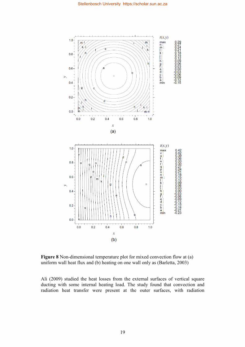
Figure 8 Non-dimensional temperature plot for mixed convection flow at (a) uniform wall heat flux and (b) heating on one wall only as (Barletta, 2003) ............................................................................................... 19
Figure 9 Variation in local Nusselt number along horizontal duct length with heated bottommost water surface (Lin et al., 1992) ............................... 20
Figure 10 Variation in local Sherwood number along horizontal duct length with heated bottommost water surface (Lin et al., 1992) .................... 24
Figure 11 Discretization schematic of the flow domain ........................................ 28
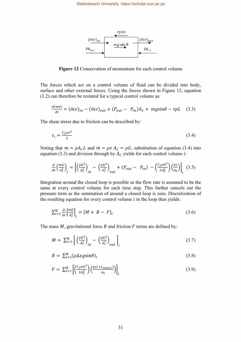
Figure 12 Conservation of momentum for each control volume ........................... 31
Figure 13 Conservation of energy for each control volume .................................. 33
Figure 14 Generalized thermal resistance network for control volume i .............. 35
Figure 15 Picture of model A (Maree, 2008) ......................................................... 39
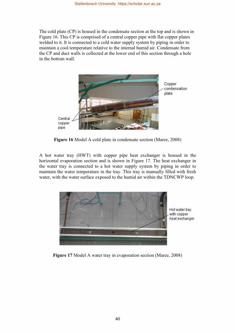
Figure 16 Model A cold plate in condensate section (Maree, 2008) ..................... 40
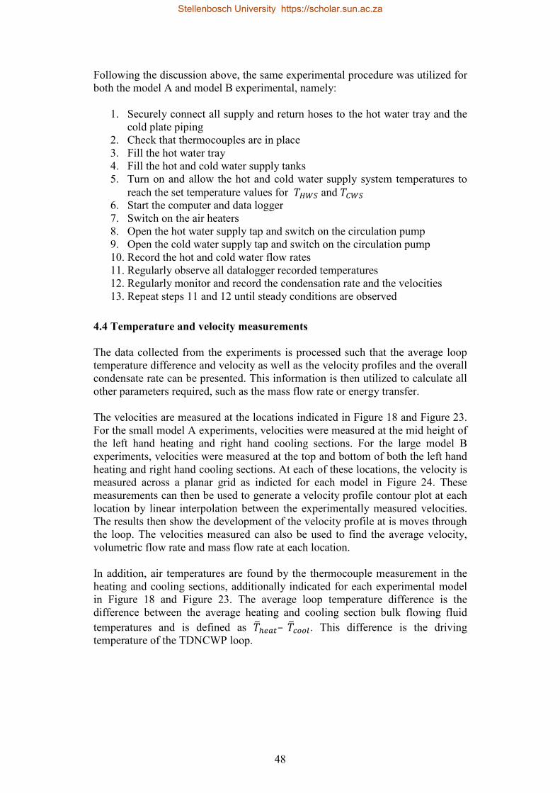
Figure 17 Model A water tray in evaporation section (Maree, 2008) ................... 40
Figure 18 Model A schematic ................................................................................ 41
Figure 19 Picture of model B ................................................................................. 42
Figure 20 Model B cold plate prior to final installation ........................................ 43
Figure 21 Model B water tray prior to final installation ........................................ 44
Figure 22 Heated wall module for model B .......................................................... 44
Figure 23 Model B model schematic ..................................................................... 45
Figure 24 Velocity measurement points with theoretical split in flow domain ............................................................................................................ 49
Figure 25 Model A loop temperature difference for Tcws = 18 °C as determined by (a) experiments and (b) numerical modelling ........................ 52
Figure 26 Model A loop temperature difference for Tcws = 10 °C as determined by (a) experiments and (b) numerical modelling ........................ 52
Figure 27 Model B temperature difference for Tcws = 18 °C as determined by (a) experiments and (b) numerical modelling ........................................... 53
Figure 28 Model B temperature difference for Tcws = 10 °C determined by (a) experiments and (b) numerical modelling ........................................... 54
Stellenbosch University https://scholar.sun.ac.za
ix
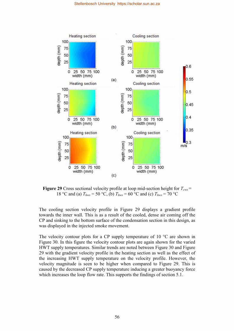
Figure 29 Cross sectional velocity profile at loop mid-section height for Tcws = 18 °C and (a) Thws = 50 °C, (b) Thws = 60 °C and (c) Thws = 70 °C ............................................................................................................... 56
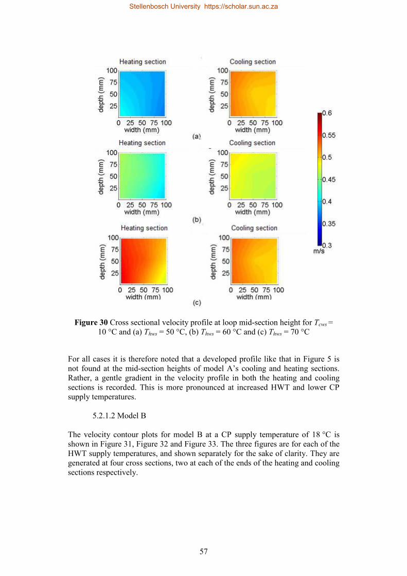
Figure 30 Cross sectional velocity profile at loop mid-section height for Tcws = 10 °C and (a) Thws = 50 °C, (b) Thws = 60 °C and (c) Thws = 70 °C ............................................................................................................... 57
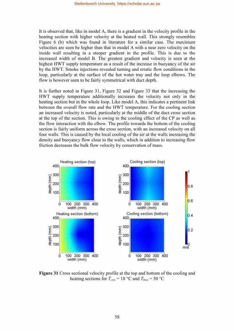
Figure 31 Cross sectional velocity profile at the top and bottom of the cooling and heating sections for Tcws = 18 °C and Thws = 50 °C .................... 58
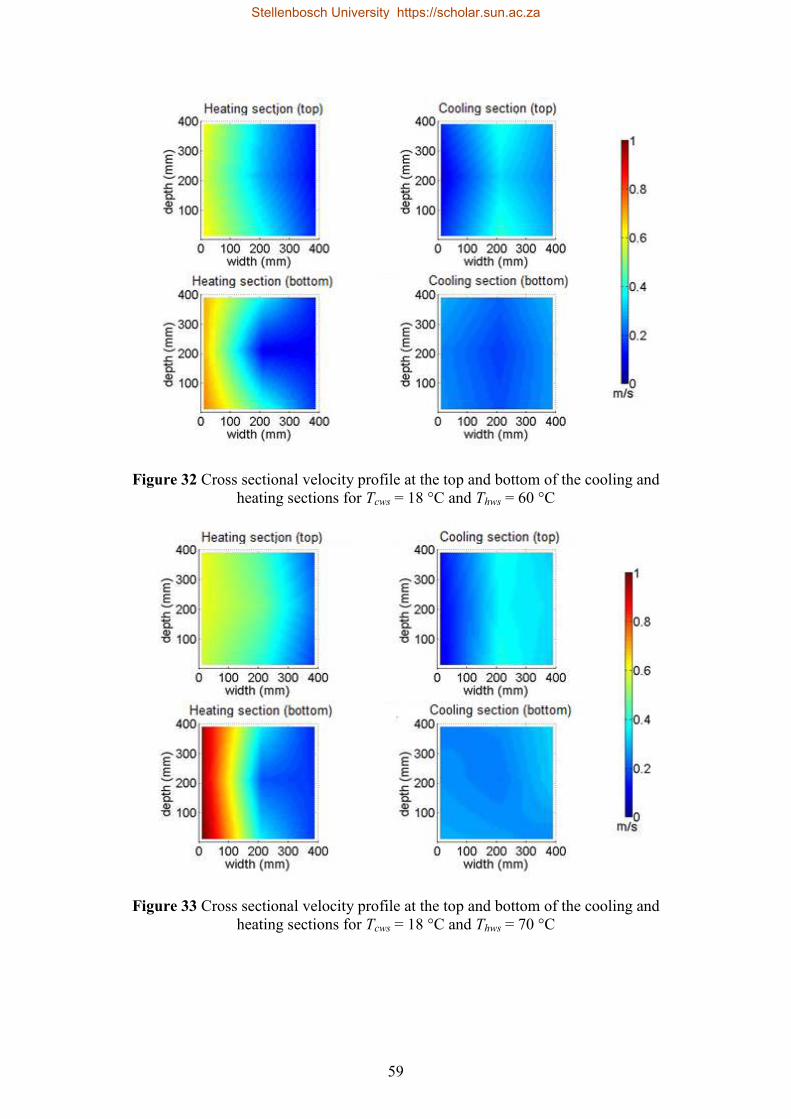
Figure 32 Cross sectional velocity profile at the top and bottom of the cooling and heating sections for Tcws = 18 °C and Thws = 60 °C .................... 59
Figure 33 Cross sectional velocity profile at the top and bottom of the cooling and heating sections for Tcws = 18 °C and Thws = 70 °C .................... 59
Figure 34 Cross sectional velocity profile normal to loop axis at the top and bottom of the cooling and heating sections for Tcws = 10 °C and Thws = 50 °C .................................................................................................... 60
Figure 35 Cross sectional velocity profile normal to loop axis at top and bottom of cooling and heating sections for Tcws = 10 °C and Thws = 60 °C ............................................................................................................... 61
Figure 36 Cross sectional velocity profile normal to loop axis at top and bottom of cooling and heating sections for Tcws = 10 °C and Thws = 70 °C ............................................................................................................... 61
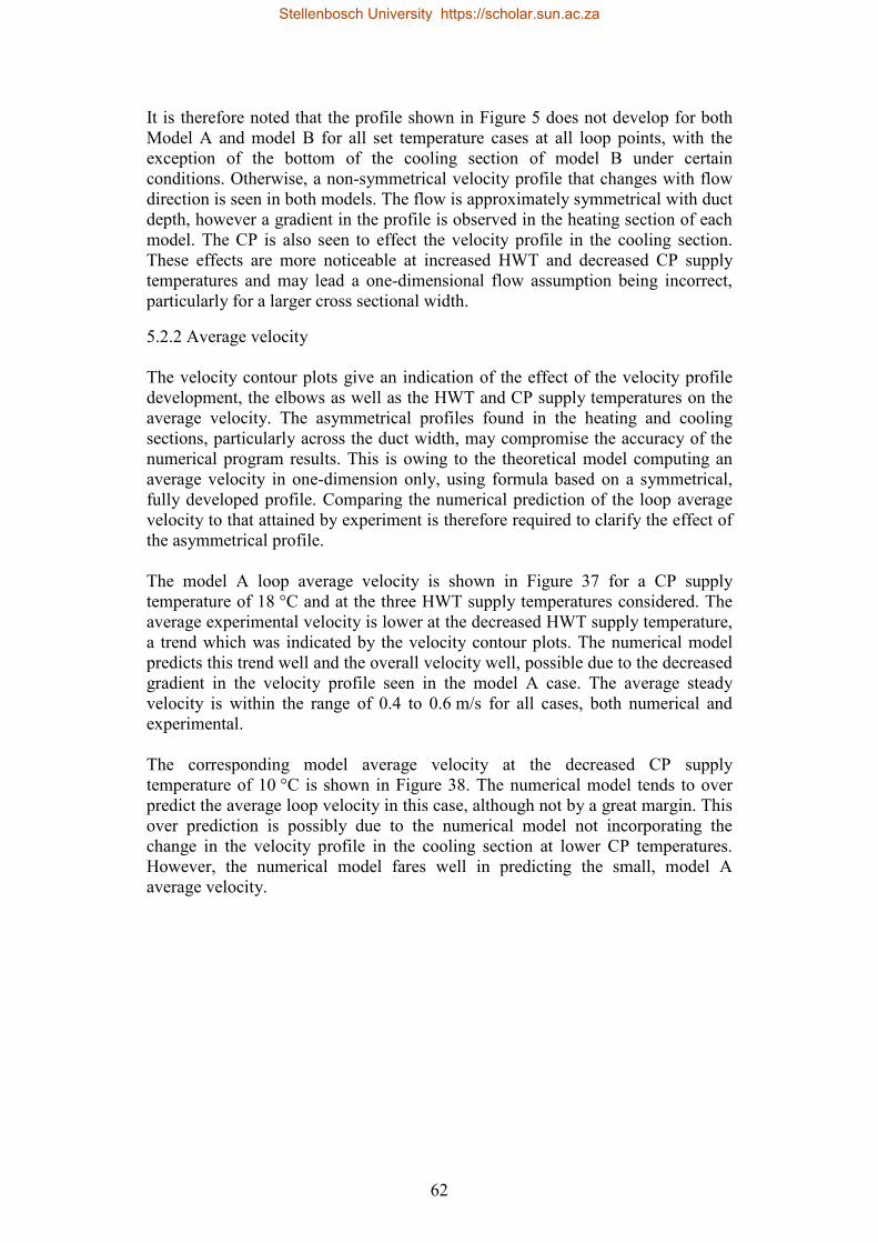
Figure 37 Model A loop average velocity for Tcws = 18 °C determined by (a) experiments and (b) numerical modelling ................................................ 63
Figure 38 Model A average loop velocity for Tcws = 10 °C as determined by (a) experiments and (b) numerical modelling ........................................... 63
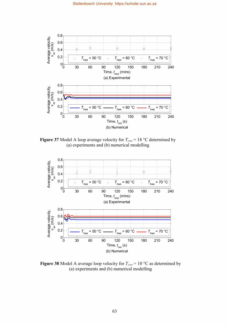
Figure 39 Model B loop average velocity for Tcws = 18 °C determined by (a) experiments and (b) numerical modelling ................................................ 64
Figure 40 Model B loop average velocity for Tcws = 10 °C determined by (a) experiments and (b) numerical modelling ................................................ 65
Figure 41 Model A condensate rate for Tcws = 18 °C as determined by (a) experiments and (b) numerical modelling ...................................................... 66
Figure 42 Model A condensate rate for Tcws = 10 °C as determined by (a) experiments and (b) numerical modelling ...................................................... 67
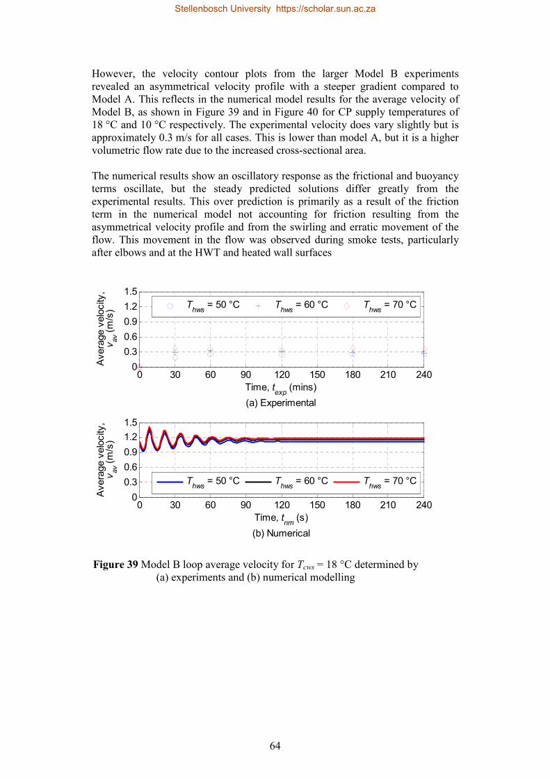
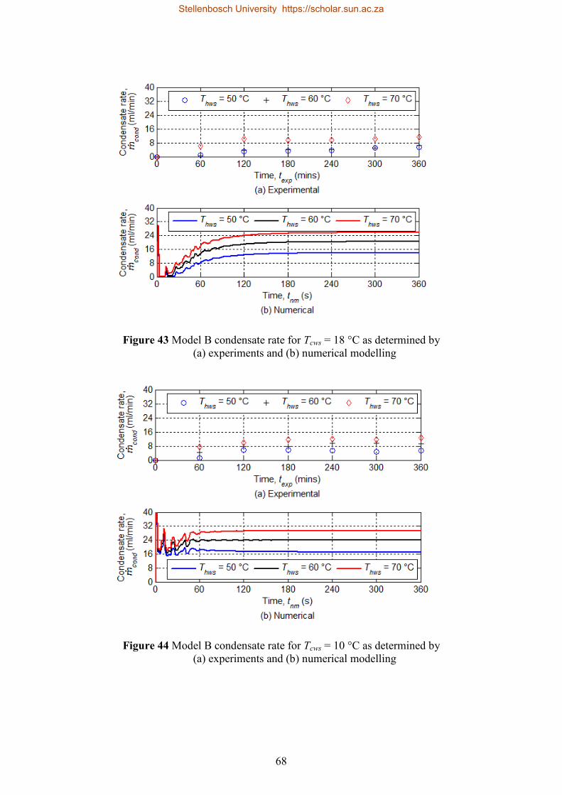
Figure 43 Model B condensate rate for Tcws = 18 °C as determined by (a) experiments and (b) numerical modelling ...................................................... 68
Figure 44 Model B condensate rate for Tcws = 10 °C as determined by (a) experiments and (b) numerical modelling ...................................................... 68
Figure 45 Model A steady water delivery per 10 hour day ................................... 69
Figure 46 Model B steady water delivery per 10 hour day ................................... 70
Figure 47 Model A energy utilization factor ......................................................... 72
Figure 48 Model B energy utilization factor ......................................................... 73
Figure 49 Condensate rate for varied duct and TDNCWP loop size at Tcws = 18 °C and Thws = 50 °C ................................................................................ 74
Figure 50 Psychometric chart demonstrating evaporative cooling process ........... 86
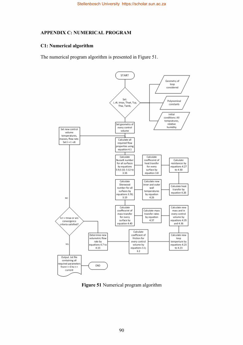
Figure 51 Numerical program algorithm ............................................................... 90
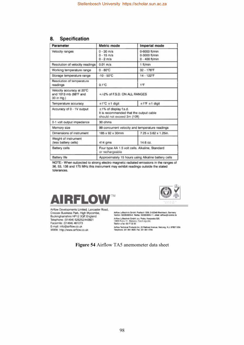
Figure 54 Airflow TA5 anemometer data sheet .................................................... 98
Stellenbosch University https://scholar.sun.ac.za
xi
LIST OF TABLES
Page
Table 1 Comparison of PDEC water requirements in buildings with varied applied loading ...................................................................................... 6
Table 2 Comparison of PDEC water requirements for various room types and climatic conditions (Kang & Strand, 2009) ............................................... 6
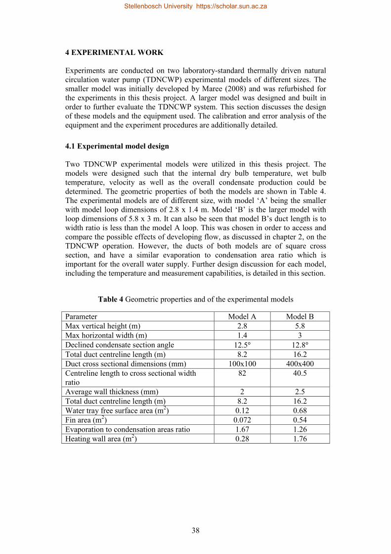
Table 4 Geometric properties and of the experimental models ............................. 38
Table 5 Experiment set temperatures ..................................................................... 47
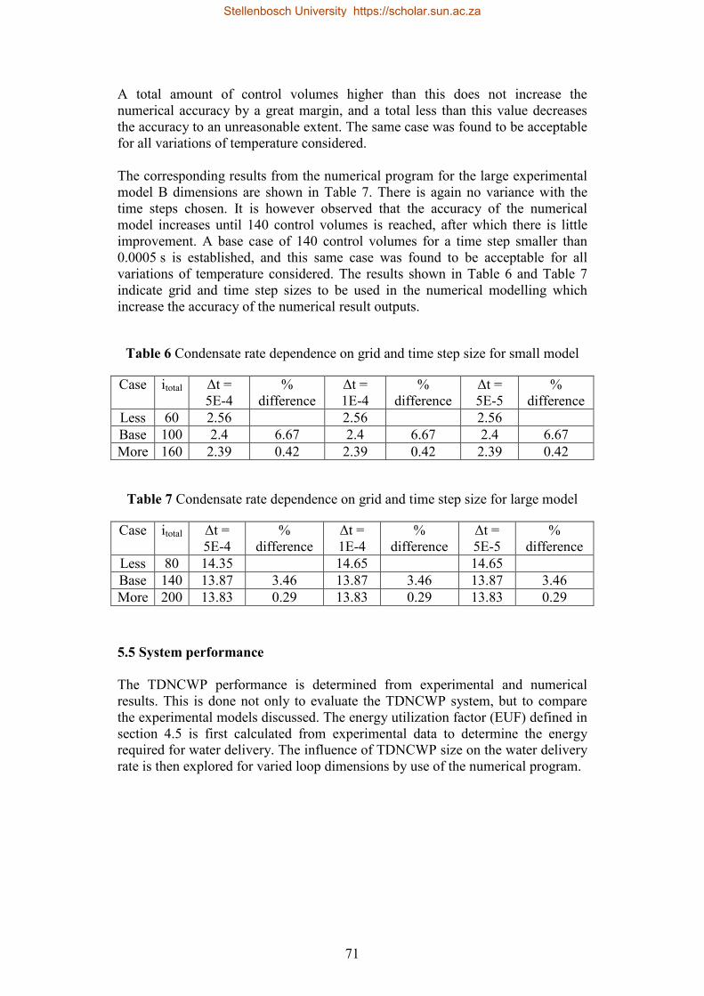
Table 6 Condensate rate dependence on grid and time step size for small model .............................................................................................................. 71
Table 7 Condensate rate dependence on grid and time step size for large model .............................................................................................................. 71
Table 8 Sample calculation of required pumping power ....................................... 87
Table 9 Energy per loop section for model A ........................................................ 88
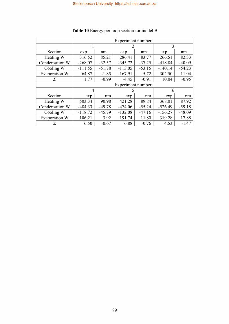
Table 10 Energy per loop section for model B ...................................................... 89
Table 11 Polynomial constants for property curve fits .......................................... 91
Table 12 Polynomial fits to calibration data for model A thermocouples ............. 93
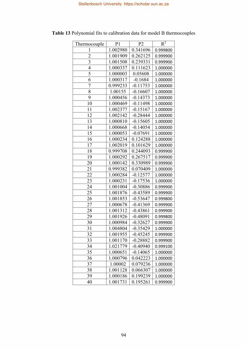
Table 13 Polynomial fits to calibration data for model B thermocouples ............. 94
Table 14 Raw calibration data ............................................................................... 95
Stellenbosch University https://scholar.sun.ac.za
xii
NOMENCLATURE
A Area B Gravitational force term C Constant CF Curve fit �� Friction coefficient �� Specific heat at constant pressure �� Hydraulic diameter ��� Diffusion coefficient for water vapour into air Total energy �� Energy utilization factor F Friction term Volumetric flow rate � Gravitational acceleration ℎ Enthalpy ℎ�� Latent heat of vaporization ℎ� Vapour saturation enthalpy ℎ�� Heat transfer coefficient ℎ�� Mass transfer coefficient � Control volume number � Conductivity � Length � Mass �� Mass flow rate � Mass term �� Molar mass �1 Momentum change term 1 �2 Momentum change term 2 � Total number of control volumes � Pressure �1 Polynomial coefficient 1 �2 Polynomial coefficient 2 � Perimeter �� Heat transfer rate Thermal resistance Gas constant of air � Gas constant of water vapour ! Temperature T1 Temperature change term 1 T2 Temperature change term 2 " Time # Internal energy $ Volume % Velocity
Stellenbosch University https://scholar.sun.ac.za
xiii
&� Work rate ' Width ( Duct length (� Mass fraction ) Height * Difference + Coefficient of volumetric expansion , Relative surface roughness - Angle relative to the horizontal . Dynamic viscosity / Density Σ Summation 1 Shear stress 2 Relative humidity 3 Specific humidity SUPERSCRIPT: % Mean %5 In all Cartesian directions " At time t Top At the top Bottom At the bottom SUBSCRIPT: 6 Air 6% Average at cross section �'7 Cold water supply � Cross section �ℎ Characteristic CS Control surface CV Control volume �8 Conductivity �9:8 Condensation �9:% Convective �99; Cooling section =(� Experimental >;#�8 Of the flowing fluid >9?�=8 Forces outside local domain ℎ' Heated wall ℎ'7 Hot water supply ℎ8 Hydrodynamic ℎ" Heat transfer
Stellenbosch University https://scholar.sun.ac.za
xiv
ℎ=6" Heating section � At control volume i �: Into control volume �::=? Inside surface ;6� In the laminar flow regime ��:9? Minor losses �" Mass transfer �! Overall into control volume :6"#?6; Due to local natural forces :� Numerical 9#" Out of control volume 9"ℎ=? Other than those specified 9#"=? Outer surface Resultant 76" At saturation condition S Maximum amount of surfaces 7 At or applied to surface 7@7 Of the entire system "� Thermocouple "#?A In the turbulent flow regime % Vapour '6;; Of the wall DIMENSIONLESS NUMBERS: Gr = �EFGH� GIJKLMNO Grashoff number
Nu = �LRJKLS Nusselt number
Pr = UVWS Prandtl number
RaZ = GrZ Pr Rayleigh number Re = \�]^ JKLW Reynolds number
Sh = �aRJKLb^]c]de Sherwood number
Sc = W\ b^]c]de Schmidt number
Stellenbosch University https://scholar.sun.ac.za
xv
ABBREVIATIONS: CP Cold plate EUF Energy utilization factor HWT Hot water tray HVAC Heating, ventilation and air conditioning LCCA Life cycle cost analysis LHS Left hand side PDEC Passive downdraft evaporative cooling RHS Right hand side TDNCWP Thermally driven natural circulation water pump
Stellenbosch University https://scholar.sun.ac.za
1
1 INTRODUCTION AND OBJECTIVES
Green building design is a manner of designing structures and using operational practices which are energy efficient, resource efficient and environmentally responsible (Green building Council of South Africa, s.a.). The design philosophy is to utilize renewable, energy conscious and sustainable design methods for buildings with a focus on reducing the energy consumption. An energy intensive practise in the built environment is that of traditional electrical air conditioning. A passive downdraft evaporative cooling (PDEC) system provides an alternative to conventional methods, using natural phenomena such as density, gravitation and evaporative cooling to condition the air ventilating a building. However, the system need water at building-roof level, which requires the use of an energy intensive, electricity driven pumping process. The thermally driven natural circulation water pump (TDNCWP) system is a passive, green building design mechanism to be used to deliver the water required for a PDEC system. The TDNCWP mechanism makes use of natural, density gradient driven air circulation and passive energy resources in manner similar to the hydrological cycle on earth. The TDNCWP has been the subject of a proof-of-concept unpublished undergraduate project by Maree (2008). It was found to be a feasible topic for further research and development. The objectives of this thesis project are to:
• Design, construct and test experimental models of the Thermally Driven Natural Circulation Water Pump (TDNCWP)
• By use of experimental data, determine the feasibility of using a simple one-dimensional theoretical model to simulate the TDNCWP system
• Evaluate the daily water delivery capabilities of the TNDCWP This report details the findings of the thesis project. The motivation for the TDNCWP system and the context of its application are first discussed. A comprehensive literature survey is then provided. The theoretical model development and experimental designs are presented, and the corresponding results detailed. Final discussions, conclusions and recommendations are then considered.
Stellenbosch University https://scholar.sun.ac.za
2
2 LITERATURE SURVEY
A literature survey on the overall system is presented. The conventional approach to building air conditioning is first explored, before a passive alternative and the TDNCWP system are introduced. As no published literature relating directly to the TDNCWP was found, the fundamental momentum, energy and mass transfer principles upon which the TDNCWP can be based are instead presented. The literature study therefore aims to provide a basis for understanding and approximating the flow conditions and is mindful of the complicated flow conditions possible. Empirical results from literature are favoured as they offer further insight into complex flow conditions. Numerical simulations are also explored in certain applications. The fluid flow conditions are explored, in particular the velocity profile and friction effects in developed and developing flow. The heat transfer mechanisms are then presented, with the different TDNCWP sections considered separately. Evaporation and condensation in the loop is then considered and discussed.
2.1 Conventional system energy usage
With the consequences of global climate change being realized, the requirement for sustainable, energy conscious design is apparent through the conservative usage of emission causing energy. This design requirement is necessary in the building sector where green house gas emissions account for 23% of the total emissions in South Africa (Milford, 2009). The application of sustainable design in the built environment has lead to the concept of so-called green building design. The methodology is to reduce the energy and life cycle resource consumption of buildings. This is achieved by increasing the efficiency and sustainability of the energy production methods for that building. It is also achieved by reducing the energy losses by improving the efficiency of the building equipment, building materials and building usage (Harvey, 2012) A conventional, energy intensive practice in the built environment is that of Heating, Ventilation and Air-Conditioning (HVAC). HVAC systems are ergonomic systems utilized with intent to improve the comfort and productivity of the occupants, as well as to maintain an air standard within health and safety regulations within building codes. HVAC systems condition the environment in a building by changing the temperature, humidity and quality of the internal air as well as the rate of air movement within the building. These systems make use of electricity driven chillers and fan-coil units as well as piping and ducts to cool and force air into and out of a building. In South Africa, the electricity used by HVAC systems is primarily generated from fossil-fuels, which produce climate changing emissions. In addition, HVAC systems are often purchased off the shelf instead of being designed and refined for the building and application conditions, and as a result they can be inefficient. This can be mitigated by the use of control systems. However, a trend analysis
Stellenbosch University https://scholar.sun.ac.za
3
performed by Austin (1997) on a typical HVAC system revealed that even with an energy management control system, unforeseen errors can occur that lead to the system operating less efficiently, and therefore using even more electricity than its design values. The actual electricity usage of HVAC systems in South Africa as stated by Eskom is around 15% of peak power consumption, or 5400 MW (Eskom demand side management, 2013). However, the specific energy usage of a typical HVAC system depends largely on the building utilization. Mathews et al. (2001) found that HVAC power consumption constituted 54% of the total building usage in an office building housing 1600 people over 4265 m2 floor area. Further to this, for specific region climatic conditions the general building usage patterns and subsequent energy usage can be categorized well by the industry the building is utilised in. In studies conducted by the City of Cape Town, it is seen that the total energy usage is over 22 000 000 GJ (2006) per annum in the commercial and industrial sectors in that city, of which 23% is in the commercial sector (2003). Moorlach & Hughes (2010) stated that approximately 27% of all electricity is utilized just for the cooling of air entering a building in the commerce sector in South Africa. HVAC can therefore constitute a large amount of a regions total energy usage. In addition to relying on fossil fuel based technologies this energy usage also has an associated financial cost. As indicated in Figure 1, a life cycle cost analysis (LCCA) presented by Fuller (2010) states that energy costs constitute 50% of typical HVAC lifecycle costs over 30 years, in addition to capital, maintenance and replacement costs.
Figure 1 HVAC system costs (Adapted from Fuller, 2010)
Stellenbosch University https://scholar.sun.ac.za
4
Despite the actual energy consumption values depending on the building type, usage, industry and annual climatic conditions, it is clear that the energy usage by current building HVAC mechanisms can be significant. By replacing these conventional means with a passive mechanism of air conditioning, overall energy usage and fossil fuel based electricity emissions could be greatly reduced.
2.2 Passive downdraft evaporative cooling
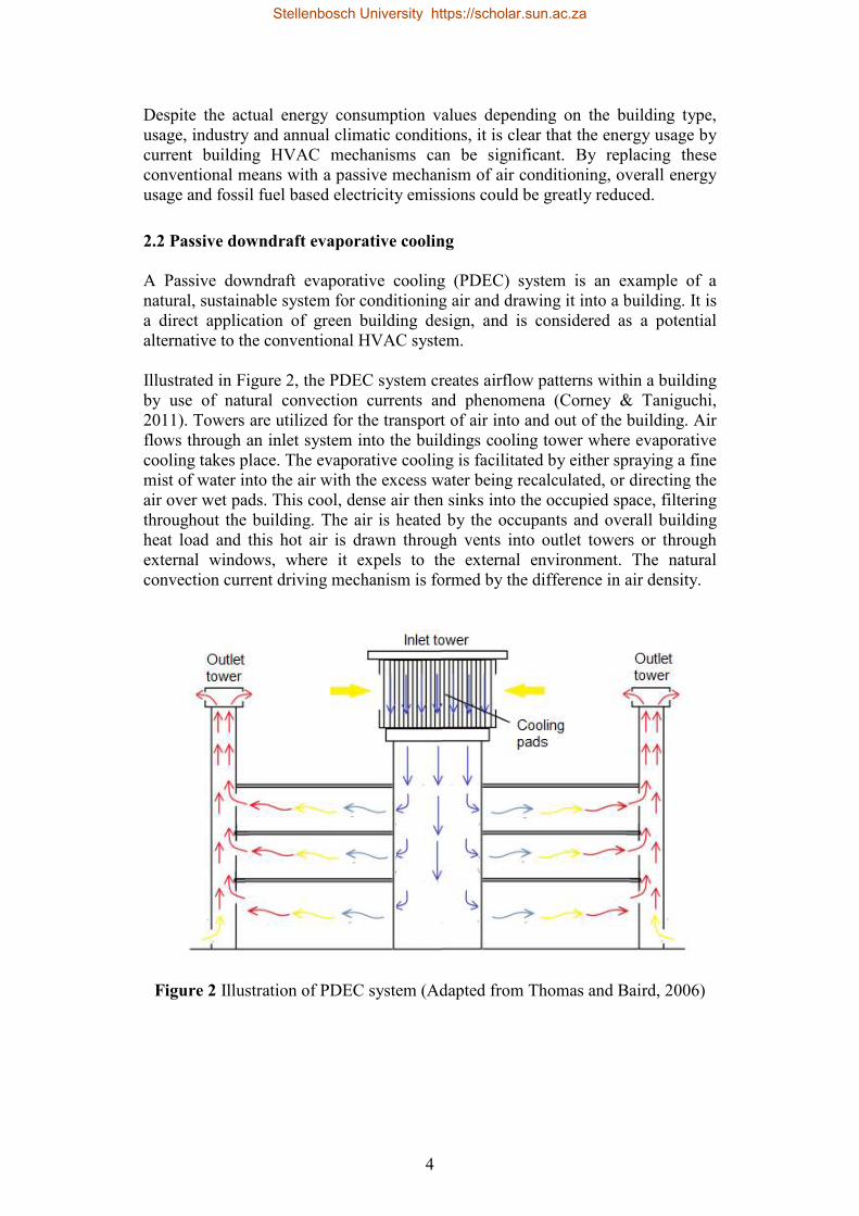
A Passive downdraft evaporative cooling (PDEC) system is an example of a natural, sustainable system for conditioning air and drawing it into a building. It is a direct application of green building design, and is considered as a potential alternative to the conventional HVAC system. Illustrated in Figure 2, the PDEC system creates airflow patterns within a building by use of natural convection currents and phenomena (Corney & Taniguchi, 2011). Towers are utilized for the transport of air into and out of the building. Air flows through an inlet system into the buildings cooling tower where evaporative cooling takes place. The evaporative cooling is facilitated by either spraying a fine mist of water into the air with the excess water being recalculated, or directing the air over wet pads. This cool, dense air then sinks into the occupied space, filtering throughout the building. The air is heated by the occupants and overall building heat load and this hot air is drawn through vents into outlet towers or through external windows, where it expels to the external environment. The natural convection current driving mechanism is formed by the difference in air density.
Figure 2 Illustration of PDEC system (Adapted from Thomas and Baird, 2006)
Stellenbosch University https://scholar.sun.ac.za
5
The evaporative cooling process in the PDEC system is a naturally occurring process and is demonstrated, in the adiabatic case, on the psychometric chart in appendix A. If the hot external air is exposed to the wet surface or a water droplet, evaporation will occur if the relative humidity of the air is less than 100%. This is the case when the wet bulb temperature of that air is less than its dry bulb temperature. As a result of the evaporation of water, adiabatic cooling of the air occurs as the latent energy required to evaporate the water is provided by a decrease in sensible energy. This reduces the dry bulb temperature of the air and can occur until it is equivalent to the wet bulb temperature of the air. At this point the relative humidity is 100% and no further cooling can occur. For this reason, PDEC systems are generally considered to be best suited to locations with a high environmental dry bulb temperature and low relative humidity. PDEC systems are often studied in the role to supplement an existing HVAC system. The Torrent research centre in Ahmedebad, India is one example of an installed PDEC system in a large, newly developed building in a region with three distinct climatic conditions per annum. The users of the building were asked in a survey to rate various aspects of comfort in this building, and the results were found to be satisfactory. A post-occupancy evaluation analysis further found that the system consumed 54 kWh/m2, which is much lower that the target of 140 kWh/m2 for newly developed buildings in India and India’s own average of 280 to 500 kWh/m2 (Thomas and Baird, 2006). The system reduced the external air temperature by an average of 5 ºC and peak of 12 to 14 ºC. Bowman et al. (1998) found that a temperature drop to within 70 to 80% of the wet bulb temperature of the inlet air is possible when sufficient water is provided to the PDEC system. The water used in the PDEC system is required at roof level, such that the water-cooled air can sink into the building. The volumetric water requirements for a PDEC system are application based and not readily available for a variety of applications. However, the water requirement findings of studies by Bowman et
al. (1998), Guedes and de Melo (2006) and Robinson et al. (2006) are summarized in Table 1. These studies are presented for a various designs, and therefore they vary in external air temperatures, required air flow rate, PDEC tower configuration, overall building size and loading, as well as desired drop in temperature. They are all presented for mister type PDEC systems. The results of these studies which are shown in Table 1 indicate that the water required to remove a unit of heating load decreases with increasing total building load. It should also be noted that with these systems, some water is not evaporated in the PDEC tower. This indicates that with a more efficient evaporation method less water would be required. Kang & Strand (2009) provided further information relating to water requirements to room types. Their findings are summarized in Table 2. It is observed that the water required per volume of cooled space decreases with increasing space volume, which supports a previous observation made on Table 1.
Stellenbosch University https://scholar.sun.ac.za
6
The water requirements for the PDEC systems are therefore shown to vary depending on the building, environment and area of application. This is much like the electrical requirements of the typical HVAC system.
Table 1 Comparison of PDEC water requirements in buildings with varied applied loading
Source Building cooled by
PDEC system
Room temperature
ºC
2
Cooling load* Water required+
Bowman et al.,
1998
4 blocks of 27 x 63 m 5-
storey buildings
27 <70 ≈8 kWh/m2 ≈1 L/day /person
27 x 70 m 4-storey
building.
26 <70 ≈20.9 kWh/m2 ≈10 L/day /person
Guedes and de Melo, 2006
19 m2 floor and 63 m3
volume with concrete walls
and 1 north facing
window. External air
temperature of 42 ºC
26.5 ≈70 ≈1.85 kWh/m2 ≈2.5 L/day /person
25.5 ≈70 ≈2.42 kWh/m2 ≈2 L/day /person
Robinson et
al., 2006
Supplementary cooling by
PDEC system
/ / ≈631 kWh/annum
≈17 L/day
*based on information given relating to building size +based on information given relating to building occupancy
Table 2 Comparison of PDEC water requirements for various room types and climatic conditions (Kang & Strand, 2009)
Room type Classroom Office Auditorium Volume m3 396 2128 7904
A water pump can be utilized to move the water required for the mister or cooling pads at roof level, which facilitate water pump, a typical PDEC system requires no electrical input and is a completely sustainable process for conditioning the air entering a building. However, the pumping of wateprocess. In a study by Kang (2011), 150 to for PDEC towers at 5 to 8m above ground. A sample calculation illustrating the pumping power required for the PDEC system by appendix B1. Use of a pump to provide the required has a high energy usage and associated cost. other electrical pump costscosts, maintenance also fois utilized, as indicated in pumped, and may vary depending on the location of the installation.
Figure 3 Typical life cycle cost
The conventional PDEC systems reliance on electricitywater further implies that if elonger be cooled. This would lead to uncomalternative to a pump system, the municipal utilized to provide the required waterand high volume of waterwould be required, and this is not always available or feasibl With energy costs that are encountered in supplying the required water for the PDEC system by use of an electrical pump, tuninterrupted and sustainableelevation is then realised
7
A water pump can be utilized to move the water required for the mister or cooling pads at roof level, which facilitate evaporative cooling. With the exception of this water pump, a typical PDEC system requires no electrical input and is a completely sustainable process for conditioning the air entering a building. However, the pumping of water to roof level is an energy intensive and expensive process. In a study by Kang (2011), 150 to 250W of pumping power was required for PDEC towers at 5 to 8m above ground. A sample calculation illustrating the pumping power required for the PDEC system by Bowman et al. (1998) is seen in
a pump to provide the required water for a typical PDEC system therefore has a high energy usage and associated cost. These energy costs, relative to all
pump costs, are shown in Figure 3. In addition to these energy costs, maintenance also forms a large portion of the cost when an electrical is utilized, as indicated in Figure 3. This also varies on the quality of the water
vary depending on the location of the installation.
cycle costs of an electrical pump (Hydraulic Institute,
PDEC systems reliance on electricity for pumping the required that if electricity supply were to fail the building would no
d. This would lead to uncomfortable working conditions. As an alternative to a pump system, the municipal water supply line couldutilized to provide the required water. However, due to the height of the towers and high volume of water required, a higher pressure water supply with piping
required, and this is not always available or feasible.
With energy costs that are encountered in supplying the required water for the PDEC system by use of an electrical pump, the motivation for a passive
sustainable alternate manner of water pumpingis then realised.
A water pump can be utilized to move the water required for the mister or cooling evaporative cooling. With the exception of this
water pump, a typical PDEC system requires no electrical input and is a completely sustainable process for conditioning the air entering a building.
nsive and expensive of pumping power was required
for PDEC towers at 5 to 8m above ground. A sample calculation illustrating the (1998) is seen in
water for a typical PDEC system therefore relative to all
. In addition to these energy electrical pump
. This also varies on the quality of the water
pump (Hydraulic Institute, 2001)
for pumping the required the building would no
fortable working conditions. As an could also be
due to the height of the towers y with piping
With energy costs that are encountered in supplying the required water for the motivation for a passive,
alternate manner of water pumping to a higher
Stellenbosch University https://scholar.sun.ac.za
8
2.3 The thermally driven natural circulation water pump
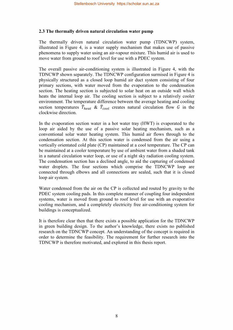
The thermally driven natural circulation water pump (TDNCWP) system, illustrated in Figure 4, is a water supply mechanism that makes use of passive phenomena to supply water using an air-vapour mixture. This humid air is used to move water from ground to roof level for use with a PDEC system. The overall passive air-conditioning system is illustrated in Figure 4, with the TDNCWP shown separately. The TDNCWP configuration surmised in Figure 4 is physically structured as a closed loop humid air duct system consisting of four primary sections, with water moved from the evaporation to the condensation section. The heating section is subjected to solar heat on an outside wall which heats the internal loop air. The cooling section is subject to a relatively cooler environment. The temperature difference between the average heating and cooling section temperatures !h�i� & !hUjjk creates natural circulation flow in the clockwise direction. In the evaporation section water in a hot water tray (HWT) is evaporated to the loop air aided by the use of a passive solar heating mechanism, such as a conventional solar water heating system. This humid air flows through to the condensation section. At this section water is condensed from the air using a vertically orientated cold plate (CP) maintained at a cool temperature. The CP can be maintained at a cooler temperature by use of ambient water from a shaded tank in a natural circulation water loop, or use of a night sky radiation cooling system. The condensation section has a declined angle, to aid the capturing of condensed water droplets. The four sections which comprise the TDNCWP loop are connected through elbows and all connections are sealed, such that it is closed loop air system. Water condensed from the air on the CP is collected and routed by gravity to the PDEC system cooling pads. In this complete manner of coupling four independent systems, water is moved from ground to roof level for use with an evaporative cooling mechanism, and a completely electricity free air-conditioning system for buildings is conceptualized. It is therefore clear then that there exists a possible application for the TDNCWP in green building design. To the author’s knowledge, there exists no published research on the TDNCWP concept. An understanding of the concept is required in order to determine the feasibility. The requirement for further research into the TDNCWP is therefore motivated, and explored in this thesis report.
Stellenbosch University https://scholar.sun.ac.za
9
Figure 4 The thermally driven natural circulation water pump illustrated (a) by itself and (b) within the complete passive air-conditioning system
Stellenbosch University https://scholar.sun.ac.za
10
2.4 Humid air flow
Interaction of the local momentum, energy and mass transfer at each section with the other sections occurs through the flow of air around the loop. The local heat and mass transfer in the loop is dependent on the flow rate, which in turn is affected by the local friction as well as the friction and heat and mass transfer everywhere else in the loop. This strong coupling of the local conditions with those everywhere else in the system complicates the development of analytical solutions as assumptions on the flow profiles cannot readily be made. It further implies that the conservation equations are applied differently to each section of the loop shown in Figure 4. The flow rate in the TDNCWP system is caused by the temperature difference between the loop’s heating and cooling systems. The temperature difference induces a buoyancy force which causes the flow of humid air within the loop. At each section of the loop this bulk fluid flow affects and is affected by the local surface heat and mass transfer. Characterising the flow conditions and velocity is therefore important in understanding the local mass and heat transfer at each section. Literature pertaining to the flow conditions and velocity is presented in this section
2.4.1 Flow characterisation Fluid flow can be categorized by what regime the fluid flow is in, namely: laminar, transition or turbulent. Laminar flow is characterized by flow which presents smooth, highly ordered motion, where turbulent flow is characterized by velocity fluctuations and very high disorder (Cengel & Cimbala, 2006). Intense mixing of the fluid is seen in these regimes, which enhances momentum, mass and energy transfer between the fluid and the surfaces. The regimes can be determined by the Reynolds number, where for internal flow if = is less than 2300 then the flow is defined as laminar Regardless of the flow regime, friction is induced by shear forces between the flowing fluid and each wall it interacts with. In straight duct lengths friction causes an overall slowing of the fluid at the wall which the bulk flow must overcome. The overall force due to friction on a body of air can be calculated from the coefficient of friction.
Stellenbosch University https://scholar.sun.ac.za
11
The Fanning coefficient of friction for fully developed internal flow is observed below (Cengel & Cimbala, 2006): ��,k� = mn.pqrs (2.1)
��,�tuv = mn wxxxy �m
m.z {|}~��.������ ���M.� ��.��������p
(2.2)
The friction induces a flow velocity profile which will develop from the leading edge of a section with constant geometric, temperature and concentration properties. The velocity profile at each section can be used to determine the average velocity at a cross section. These are related to the mass flow rate of the internal air by (Cengel and Cimbala, 2007):
%� = � \��5 ����K \�� = ��\�� = �� (2.3)
An example of the development of an ideal velocity profile inside a typical duct system is shown in Figure 5. This occurs for uniform inlet and constant wall conditions, and the development is similar for temperature and concentration profiles of the fluid.
Figure 5 Development of typical velocity boundary layer in duct flow (Adapted from Cengel& Ghajar, 2011)
With an infinitely long duct under constant wall conditions the symmetrical, fully developed profile shown in Figure 5 will eventually result for the velocity, with symmetrical profiles developing for the temperature and concentration as well. The length before the fully developed flow condition is referred to as the entry length of the flow.
Stellenbosch University https://scholar.sun.ac.za
12
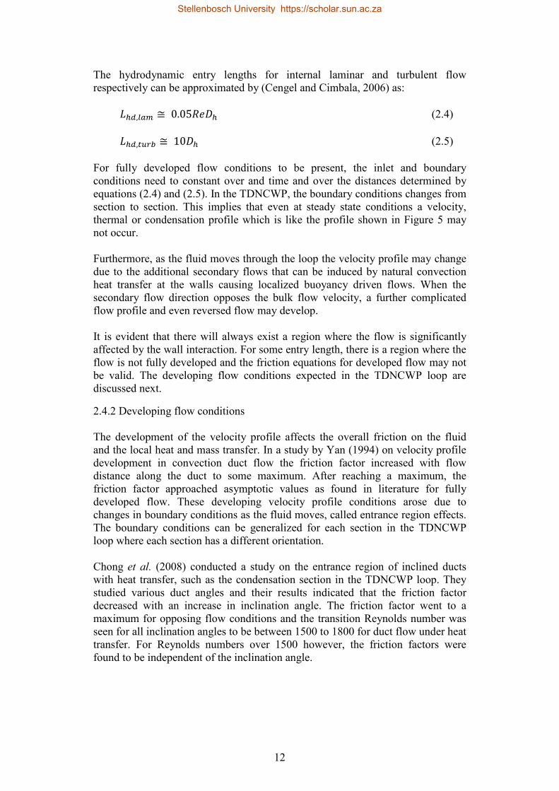
The hydrodynamic entry lengths for internal laminar and turbulent flow respectively can be approximated by (Cengel and Cimbala, 2006) as: ���,k� ≅ 0.05 =�� (2.4)
���,�tuv ≅ 10�� (2.5) For fully developed flow conditions to be present, the inlet and boundary conditions need to constant over and time and over the distances determined by equations (2.4) and (2.5). In the TDNCWP, the boundary conditions changes from section to section. This implies that even at steady state conditions a velocity, thermal or condensation profile which is like the profile shown in Figure 5 may not occur. Furthermore, as the fluid moves through the loop the velocity profile may change due to the additional secondary flows that can be induced by natural convection heat transfer at the walls causing localized buoyancy driven flows. When the secondary flow direction opposes the bulk flow velocity, a further complicated flow profile and even reversed flow may develop. It is evident that there will always exist a region where the flow is significantly affected by the wall interaction. For some entry length, there is a region where the flow is not fully developed and the friction equations for developed flow may not be valid. The developing flow conditions expected in the TDNCWP loop are discussed next.
2.4.2 Developing flow conditions The development of the velocity profile affects the overall friction on the fluid and the local heat and mass transfer. In a study by Yan (1994) on velocity profile development in convection duct flow the friction factor increased with flow distance along the duct to some maximum. After reaching a maximum, the friction factor approached asymptotic values as found in literature for fully developed flow. These developing velocity profile conditions arose due to changes in boundary conditions as the fluid moves, called entrance region effects. The boundary conditions can be generalized for each section in the TDNCWP loop where each section has a different orientation. Chong et al. (2008) conducted a study on the entrance region of inclined ducts with heat transfer, such as the condensation section in the TDNCWP loop. They studied various duct angles and their results indicated that the friction factor decreased with an increase in inclination angle. The friction factor went to a maximum for opposing flow conditions and the transition Reynolds number was seen for all inclination angles to be between 1500 to 1800 for duct flow under heat transfer. For Reynolds numbers over 1500 however, the friction factors were found to be independent of the inclination angle.
Stellenbosch University https://scholar.sun.ac.za
13
The velocity profile for vertical square duct flow was studied by Barletta et al. (2003) in their numerical work. The velocity profiles for the case of uniform heat flux at all walls and the case of one heated wall with the remaining adiabatic is shown in Figure 6.
Figure 6 Non-dimensional velocity plot for square duct with mixed convection flow at (a) uniform wall heat flux on all walls and (b) heating on one wall only
(Barletta, 2003)
Stellenbosch University https://scholar.sun.ac.za
14
An axisymmetrical profile with 4 local maxima is observed in Figure 6 (a) for the uniform heating case, and a bias profile is observed in Figure 6 (b) in the case of one heated wall. These cases are similar to those expected in the TDNCWP at the cooling and the heating sections respectively. For vertical duct flow, Oulaid et al. (2010) numerically studied vertical humid air flow with mass transfer to and from the walls. The walls were maintained at a temperature cooler than that of the air, similar to the cooling section of the TDNCWP system. The study showed that when condensation mass transfer took place this caused an opposed flow force, which created a larger boundary layer, slow heat transfer and reduced the friction factor. Down-stream of this, the velocity approached asymptotic values. For the case with one heated wall, observed in Figure 6 (b), a biased profile towards the heated wall is observed. This is due to the local buoyancy induced secondary flows being greater at that wall. Low velocity reversed flow is seen on the opposite wall. For horizontal ducts the local heat driven secondary flow combined with the entrance effects can greatly affect the bulk fluid flow. Chou (1989) studied the effects of non-uniform heating in the entrance region of horizontal square ducts, similar to the evaporation section. A secondary flow was seen to develop from the heated surface and the magnitude increased with increasing Rayleigh number or surface temperature. The friction relative to pure forced heat transfer case also increased, indicating that a higher surface temperature and associated secondary flows act to increase flow friction. In addition, the friction factor magnitude oscillated at near entrance regions, and approached an asymptotic value further along the duct. In addition to entrance effects, flow into each section is further influenced in the TDNCWP loop by the elbows at the section interfaces. The effect of elbows and the use of guide vanes is demonstrated by CFD snapshot of velocity contours in Figure 7, as presented by Smith (2013). A large area of slowed velocity is observed on the inside wall for the case without guide vanes due to the recirculation flow area. Without guide vanes a large gradient is seen in the velocity profile at a cross section of the duct downstream of an elbow. The volumetric and mass flow on the outside of the corner is therefore increased and the flow is mixed. This effect also utilizes flow energy by inducing a pressure drop and frictional loss, which can be reduced by the use of guide vanes. The frictional loss in elbows in ducts is accounted for by the addition of an equivalent straight duct or ����ju , which can be found in literature (Cengel & Cimbala, 2006).
Stellenbosch University https://scholar.sun.ac.za
15
Figure 7 Effect of elbows in duct flow (Smith, 2013)
An additional consideration for computing the flow friction and understanding the fluid flow is the variation of fluid properties. This variation occurs when the temperature or the humidity of the air changes. The effects of changing the humid air temperature was investigated for the dynamic viscosity property of air flow by Nonino et al. (2006). It was found for laminar forced convection that the effects of temperature dependent viscosity could not be neglected for all duct cross sections considered over a wide range of operatng conditions. The effects of changing the fluid humidity was investigated by Tsilinngiris (2007). It is reported that the density can be calculated from ideal gas relations and the specific heat can be calculated using the vapour mass fraction. However, the dynamic viscosity and conductivity require a modified form of the mass fraction to take into account the molecular interactions between air and vapour in a binary homogenous gas mixture. The thermal diffusivity and Prandtl numbers could then be calculated using their definitions. These varying fluid properties, coupled with the effects of developing flow complicate the computation of the friction in the TDNCWP loop. Elbows also tend to vary the flow conditions at the inlet of each section. However, the friction experienced by the fluid and overall velocity profile is a result of the flow velocity or mass flow rate gained by the heat and mass transfer everywhere else in the loop. These heat and mass transfer effects can be generalized for each section in the loop, and are discussed in subsequent sections so a further understanding of these elements is required.
Stellenbosch University https://scholar.sun.ac.za
16
2.5 Heat transfer mechanisms
Heat transfer in the TDNCWP system is caused by the wall temperature relative to the internal and external air temperatures. It is required to induce the fluid flow and increase the humidity of the humid air in the loop. The primary method of energy transfer within the TDNCWP loop is the heat transfer. Energy is also transferred by phase-change when water evaporates to or condenses from the air. Similar to the velocity profile, the air temperature profile in the loop tends to a symmetrical flow profile if there are constant inlet properties as well as velocity, mass and wall properties over a flow distance. The profile therefore redevelops when there is a change in heat transfer or physical boundary conditions from section to section, or through possible mixing due to elbows or secondary, locally induced flows. Understanding the heat and energy transfer is important in understanding the overall operation of the TDNCWP loop. Literature pertaining to this is presented in this section
2.5.1 General heat transfer Convection heat transfer takes place between the TDNCWP walls and the external and internal air. This convection is the heat transfer thorough adjacent layers of moving fluid on the internal and external surfaces of the TDNCWP walls. The heat is conducted through the wall between these two surfaces. The conduction and convection mechanisms can be defined (Cengel & Ghajar, 2011) by: ��U� = −��kt����� ��G� ¡ (2.6)
��Uj�� = ℎ��,¢ ���,¢£!¢ − !¤ (2.7) The coefficient of heat transfer is determined by finding the Nusselt number of the flow. The Nusselt number is the ratio of the magnitude of the convection heat transfer through some characteristic distance with the conductivity of that fluid. The Nusselt number can then be mathematically defined as: Nu = �LR JKLS¥¦§d¨ (2.8) To determine this Nusselt number, it must first be determined how the fluid flow is initiated. If the fluid flow is caused to move by external forces outside the local flow domain considered, the flow is said to be subjected to forced convection heat transfer.
Stellenbosch University https://scholar.sun.ac.za
17
The Nusselt number for internal flow forced convection can be found (Cengel & Ghajar, 2011) by: Nu = 2.98 (2.9) FRe < 2300I
Nu = 0.023Re® PrM (2.10) FRe > 10000; 0.5 < Pr < 2000I If the flow is caused by the body-forces in the local flow domain, such as local buoyancy, the flow is said to subject to natural convection heat transfer. The Nusselt number for external flow natural convection varies according to the orientation of the surface and is presented in Table 3. These equations, along with those for forced convection, were found by experimental observations on fully developed flow conditions. The Prandtl number and Grashoff number are found by definition. An increasing Grashoff number increases the natural heat transfer and may therefore lead to higher magnitude secondary flow.
Upper surface of a horizontal hot / lower surface of a horizontal cooled plate:
Nu = 0.54FGrZPrI� (2.11) F10n < GrZPr < 10³I Nu = 0.15FGrZPrI�M (2.12) F10³ < GrZPr < 10mmI
Lower surface of a horizontal hot / upper surface of a horizontal cooled plate:
Nu = 0.27FGrZPrI� (2.13) F10µ < GrZPr < 10mmI
Vertical plate and inclined surfaces:
Nu = 0.59FGrZPrI� (2.14) F10n < GrZPr < 10¶I Nu = 0.1FGrZPrI�M (2.15) F10m· < GrZPr < 10mqI
Stellenbosch University https://scholar.sun.ac.za
18
In addition to convection and conduction, the movement of energy is also caused by phase-change transfer, due to the enthalpy of the water molecule changing as it changes between liquid and vapour phase. The amount of heat transfer may therefore be expressed by the following (Cengel & Ghajar, 2011) where the latent enthalpy of vaporization ℎ�� can be found in property tables: ���� = �� ��ℎ�� (2.16) The heat transfer formulae for the mechanism in the TDNCWP are presented in this section for fully developed flow conditions with constant boundary and inlet conditions. However, as the flow within the TDNCWP may not be fully developed, the effect of the various boundary conditions on the internal humid air temperature requires discussion.
2.5.2 Heat transfer in the loop The bulk loop flow is due to temperature difference across the loop. However, the local temperature profile within the loop varies with the local friction as well as heat and mass transfer induced secondary local flows which can develop due to local heating. These will interact with the bulk flow. The flow conditions also depend on the orientation of the duct. For the vertical heating and cooling sections of the TDNCWP, the temperature profile was found by Barletta et al. (2003) in their numerical work. They found the temperature profiles for the case of uniform heat flux at all walls and the case of one heated wall. The results of these cases are shown in Figure 8 and are similar to that expected in the TDNCWP for the cooling and the heating sections respectively. An axisymmetrical profile is observed in Figure 6 for the former case, and a biased profile towards the heated wall in the latter. This trend is similar in the velocity profiles discussed previously. The effects of increasing the vertical channel width were investigated in a numerical study for forced and natural convection by Anand and Kim (1990). They found that the resistance to heat transfer increased with increasing width and that the resulting reduction in temperature increase along the channel impeded the local buoyancy flow effects. Shai & Barnetta. (1986) observed that for vertical duct flow that when the secondary flow assisted the bulk flow this tended to increase the boundary layer thickness. This decreased the inviscid, bulk flow region velocity, which decreased the overall heat transfer, with the opposite true for opposing flow.
Stellenbosch University https://scholar.sun.ac.za
19
Figure 8 Non-dimensional temperature plot for mixed convection flow at (a) uniform wall heat flux and (b) heating on one wall only as (Barletta, 2003)
Ali (2009) studied the heat losses from the external surfaces of vertical square ducting with some internal heating load. The study found that convection and radiation heat transfer were present at the outer surfaces, with radiation
Stellenbosch University https://scholar.sun.ac.za
20
comprising around 21% of input heat power. The analysis therefore found higher magnitude Nusselt numbers than those predicted by those proposed by Cengel and Ghajar (2011) for vertical flat plates. The vertical heated and cooling sections considered are joined at ground level to the horizontal evaporation section. For a duct with the heated bottom surface, the buoyancy induced secondary flows are orthogonal to the primary flow direction and have a greater affect on the bulk flow. Lin et al. (1992) found that the precursor to the development of these secondary buoyancy driven flows is the development of longitudinal vortex rolls. These rolls act to enhance heat transfer, induce early transition to the turbulent flow regime and cause an oscillation in the magnitude of the total Nusselt number along the duct length. Additional research on the secondary flow effects in the entrance region of ducts was conducted by Chou (1989) for horizontal square ducts. The results indicated that the strength and pattern of the secondary flow is sensitive to the circumferential distribution of wall heat flux. This local Nusselt variation along a horizontal duct is demonstrated in Figure 9 as found by Lin et al. (1992), for adiabatic walls with a heated water film at the bottom surface.
Figure 9 Variation in local Nusselt number along horizontal duct length with heated bottommost water surface (Lin et al., 1992)
Stellenbosch University https://scholar.sun.ac.za
21
The onset of secondary flows is observed in Figure 9 at the minimum Nusselt value which acts to increase the magnitude and induce oscillations. It is noted that no oscillations are seen for pure force convection case. Although heat transfer from the wetted surface does occur due to convection effects, heat transfer from the wetted wall was found by Lin et al. (1992) to be dominated by latent heat transfer associated with evaporation. The onset point of instability was also observed to occur closer to the duct entrance for a higher water temperature as well as lower inlet air humidity. This is indicative that an increased mass transfer rate induces additional local secondary, buoyancy driven flow. However, these studies did not consider the external surface heat transfer from horizontal ducts. Ali (2007) studied natural convection from the outside of horizontal duct sections of varied aspect ratios. The study found that the Nusselt number increased with increasing distance from the end of the duct section for a fixed heat flux. He further found that radiation heat transfer from the outside of the ducts was at maximum 25.5% of the total inputted heat load. The correlation developed from the experimental data are of a similar form to those for natural convection from a horizontal flat plate. With the cooling, heating and evaporation sections considered the declined condensation section at roof level remains. Chong et al. (2008) studied the thermal entrance region of inclined ducts in which they tested various angles between vertical opposing and vertical assisting flow with an internal heat source. They found that for a fixed Grashoff number and increasing Reynolds number the Nusselt number not only increased for all inclination angles but became independent of inclination angle at some Reynolds number. This was due to the secondary flow becoming negligible. Incropera and Maughan (1987) experimentally studied buoyancy aided flow in inclined ducts, for the case of heating air in inclined parallel plate flow heated from below. Relative to the case of horizontal flow, they found that the buoyancy force in the direction of the flow increased the heat transfer coefficient by 15% for an angle of 30º before the onset of Nusselt number instability. This further increased with increasing heat transfer rate. They observed that the instability point moves upstream with increasing Grashoff number and decreasing Reynolds number, corresponding to the horizontal and vertical cases observed in other studies. Correlating the data to the flow angle was not seen to be possible, due to the complex flow interaction changes with angle. Mass transfer with the walls, as expected in the TDNCWP loop condensation section, was considered by Yan (1994). The effects of simultaneous convection heat and mass transfer in inclined rectangular ducts was studied, where the walls in this study were subjected to uniform heat and mass flux. It was observed that the Nusselt number declined at the entrance region of the duct before secondary
Stellenbosch University https://scholar.sun.ac.za
22
flows influenced the flow regime and causing the Nusselt number to oscillate. Like the horizontal case, this approached an asymptotic value with increased duct length. Another consideration in the condensation section is the effect of the cold plate (CP) will cool the air flowing around it. An experimental study of the effects of heat transfer for a vertical orientated wall of a duct was conducted by Gau et al. (2000). They found that local secondary flows did develop and tended to move the cooled or heated fluid in the corners. This decreased the heat transfer from the walls in that region. They found the Reynolds number variation did not affect the accumulated flow location or size. It is therefore clear that the convection heat transfer magnitudes vary from TDNCWP section to section. The orientation of the duct affects the onset of the secondary flow conditions, which affects the Nusselt number near the duct entrance. However the Nusselt number tends to an asymptotic, forced convections solution with increased duct distance, or indeed at larger Reynolds or smaller Grashoff numbers. With the heat transfer and fluid flow conditions better understood, the mass transfer mechanisms are discussed.
2.6 Mass transfer mechanisms
In the TDNCWP loop mass transfer primarily occurs at two locations: the water-air surface at the HWT where water vapour is evaporated to the internal humid air and at the CP surface where water vapour is condensed from the humid air. At both surfaces simultaneous heat and mass transfer occurs. Mass transfer may also occur on all the internal surfaces of the loop if the conditions are favourable. Mass transfer relations by Cengel & Ghajar (2011) are developed for free surface mass transfer to and from humid air. The relations are based on the analogy that both mass and heat transfer mechanism are similar in that they occur due to diffusion and advection of mass and heat respectively. Their approach is therefore to utilize equations developed for heat transfer as a basis for similar relations for mass transfer. Mass transfer by evaporation and condensation may therefore in general be expressed by the following:
�� �� = ℎ�� ��� ¸/�,¢�@GH − /�@G]deº (2.17)
It can be seen that the mass transfer depends on a surface area, the driving property difference in vapour density at the surface which is a function of the air temperature and vapour pressures available in literature. The mass transfer coefficient is a function of the dimensionless Sherwood number. This dimensionless number corresponds to the Nusselt number in heat transfer relations, and represents the effectiveness of mass convection from a surface.
Stellenbosch University https://scholar.sun.ac.za
23
The equations for the forced convection Sherwood number (Cengel & Ghajar, 2003) are:
»ℎ = 2.98 (2.18) F = < 2300 I »ℎ = 0.023 =® »�� (2.19) F = > 10000I
The formulae are presented by Cengel & Ghajar with the caution that they may have limited accuracy as they are limited to empirical relations for certain geometries and flow conditions. The water in the evaporation section in the TDNCWP is evaporated from a free-water surface to the humid air. Sartori (2000) provides a summary of widely available correlations for evaporation from a free water surface to forced, turbulent flowing humid air. The results concluded that widely published equations which do not take into account the relative humidity of the air did not accurately predict the evaporation rates. The study further proposed that for turbulent flow conditions there was a decay in the mass transfer rate proportional to �¢�·.p. Asdrubali (2009) conducted experimental work on laminar flow over water surfaces and found that the evaporation rate increased with increasing pool temperature and with decreasing room humidity. A high sensitivity to the water temperature and flow velocity was found, with small magnitude improvements in velocity leading to much higher evaporation rates. Further research into the evaporation rates under various conditions was conducted by Smith (1993) (1999), where experimental tests on still and disturbed water surfaces pools were conducted. These results were then correlated to the phase-change energy equation (2.17). In his formulations factors are included which take into account local barometric pressure and the increase in pool area due to the agitation of the surface. Shah (2002) (2003) provides similar equations, which instead utilize the density difference shown in equation (2.17). Factors are included to account for surface agitation as well as the changing density difference. In addition, Moghiman & Jodat (2007) studied the effects of both forced evaporation due to air flow and free convection due to local density difference. They found that both mechanisms caused evaporation to occur for velocities of 0.1 to 0.3 m/s. Free surface and swimming pool heat and mass transfer provide insight into possible evaporations conditions in the TDNCWP loop. However, the evaporation rates for internal flow inside rectangular ducts were experimentally studied by Iskra & Simonson (2007) for internal humid air flow over a wet tray. This is similar to the boundary conditions in the evaporation section.
Stellenbosch University https://scholar.sun.ac.za
24
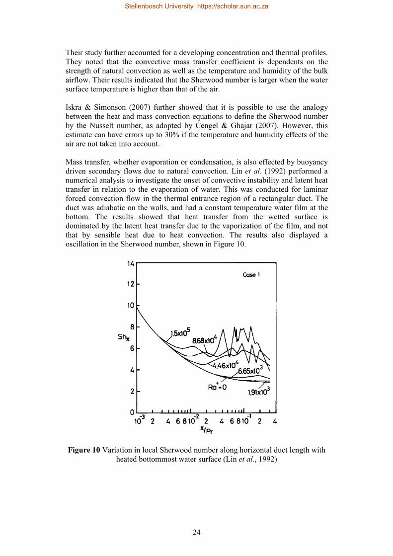
Their study further accounted for a developing concentration and thermal profiles. They noted that the convective mass transfer coefficient is dependents on the strength of natural convection as well as the temperature and humidity of the bulk airflow. Their results indicated that the Sherwood number is larger when the water surface temperature is higher than that of the air. Iskra & Simonson (2007) further showed that it is possible to use the analogy between the heat and mass convection equations to define the Sherwood number by the Nusselt number, as adopted by Cengel & Ghajar (2007). However, this estimate can have errors up to 30% if the temperature and humidity effects of the air are not taken into account. Mass transfer, whether evaporation or condensation, is also effected by buoyancy driven secondary flows due to natural convection. Lin et al. (1992) performed a numerical analysis to investigate the onset of convective instability and latent heat transfer in relation to the evaporation of water. This was conducted for laminar forced convection flow in the thermal entrance region of a rectangular duct. The duct was adiabatic on the walls, and had a constant temperature water film at the bottom. The results showed that heat transfer from the wetted surface is dominated by the latent heat transfer due to the vaporization of the film, and not that by sensible heat due to heat convection. The results also displayed a oscillation in the Sherwood number, shown in Figure 10.
Figure 10 Variation in local Sherwood number along horizontal duct length with heated bottommost water surface (Lin et al., 1992)
Stellenbosch University https://scholar.sun.ac.za
25
A high Sherwood number as observed in Figure 10 was seen near the leading edge where secondary flows were lower. Oscillations or instabilities in the Sherwood number were seen further along the duct length and eventually an asymptotic value was reached. In addition to evaporation, condensation mass transfer also occurs in the TDNCWP loop. Condensation will occur on a cooled surface in a duct when the vapour mass fraction at the duct inlet is higher than the corresponding saturation value at the wall temperature of that section (Hammou et al., 2004) In this manner, condensation occurs in the exact opposite case to that of evaporation. Surface condensation follows the same principles as evaporation, as they depend on the same properties of the air and surface. It occurs in the TDNCWP loop when warm, humid air is exposed to a relatively cooler surface at the surface of the CP in the condensation section. This also may occur on any of the inside wall surfaces of the loop. Condensation on internal walls or surfaces occurs by two means: drop-wise condensation and film condensation (Cengel & Ghajar, 2007). In drop-wise condensation, condensed water vapour forms many droplets of varied diameter on a surface. In film condensation, a continuous film forms which acts under the influence of gravity on a vertical surface. This film may have a varied thickness depending on its interaction with the flowing air and gravity, and provides a further resistance layer to heat transfer. However, in drop-wise condensation each drop eventually reaches a certain size before the gravitational force pulls the drop along the surface which exposed the surface. This allows for a higher heat transfer rate through that surface. In the TDNCWP loop however, humid air is present and not pure water vapour, and the air present may in itself effect the formation of film or drop wise condensation. In addition to the mass transfer formulae and discussion presented previously, condensation of water vapour from humid air in ducts was numerically studied by Hammou et al. (2004). In their configuration, air with uniform dry bulb temperature, humidity and velocity as well as fixed Reynolds and Schmidt numbers entered a channel. They found that the Nusselt and Sherwood profiles across the channel had a similar profile and magnitudes due to the Schmidt and Prandtl numbers being nearly equivalent. This supports the approach supplied by Cengel & Ghajar. The study further indicated that the Sherwood increases with increasing inlet temperature and specific humidity. In a similar study on condensation in duct flow for vertical rectangular ducts with condensation at one of the walls, Huang et al. (2004) found that the condensation rate at the surface decreased with increasing humid air relative humidity, due to the diffusion rate of the water vapour in the air. This was conducted for a laminar Reynolds number at an unspecified velocity.
Stellenbosch University https://scholar.sun.ac.za
26
For condensation on the CP, Cheng & Junming (2011) conducted an investigation on the humid air flow over a cooled vertical flat plate. They found that the condensate rate increased as a nearly linear function of increasing velocity between 0.5 to 3 m/s, and that this function had a higher growth rate at higher inlet humidity ratios. Coney et al. (1988) also considered condensation from humid air to a flat plate. They observed that for a fixed relative humidity the condensate rate increased with increasing air temperature. This was due to the absolute humidity increasing, as warmer air can contains a higher mass of water vapour. The overall mass transfer rate at a surface varies with the flowing air conditions such as the relative and specific humidity, the pressure, temperature, velocity, flow regime and its physical interaction with the surface. It also varies with the characteristics of this surface such as the temperature, exposed area and smoothness of the mass transfer surface. Although the governing principles for condensation and evaporation are generally the same, there are specific mechanisms of condensation and they affect the heat transfer rate on that surface. However, the mass-heat transfer analogy is proposed. These concepts, combined with those found for the flow conditions and heat transfer in the loop, provide a good understanding of the mechanism of the TDNCWP loop.
2.7 Chapter summary
The motivation for research on the TDNCWP and the literature survey were presented in this chapter. As there exists no published data on the TDNCWP, this literature survey could not be conducted on the whole system. It therefore focused on the various component systems in the TDNCWP system. In chapter 3, the formulae and information found is applied with the conservation equations to develop a theoretical model.
Stellenbosch University https://scholar.sun.ac.za
27
3 THEORETICAL MODEL
Using the theory presented in the literature survey in chapter 2, a one-dimensional theoretical model of the thermally driven natural circulation water pump (TDNCWP) is developed. A numerical model is then generated which is based on this theoretical model and the TDNCWP configuration discussed in section 2.3. This is used to simulate the flow conditions within the TDNCWP loop and predict the overall water supply output. In this section the theoretical model development is detailed. First the developmental assumptions are discussed, before the momentum transfer, mass transfer and heat transfer equations are presented based on the findings of the literature review. The discretization of these equations for use in the numerical model is further detailed. Finally, the system mass changes are discussed.
3.1 Developmental assumptions
Theoretical model equations are developed based on fundamental theories. Numerical simulation solves the theoretical model equations across small control volumes. These control volumes are formed by discretizing the entire flow domain around the TDNCWP loop into � computational domains. This is demonstrated in Figure 11. The humid air mixture in the loop is exposed to a variety of boundary conditions: a heated wall; a cold plate (CP); a hot water surface at the water tray (HWT); as well as a varying wall temperature around the loop. The theoretical model therefore aims to incorporate the heat transfer at these locations, as well as mass transfer at particular locations in the loop. Each control volume in the numerical model has a unique set of initial, boundary and internal conditions which are utilized to solve the coupled heat transfer, mass transfer and momentum change equations at that control volume. A time dependent model with an explicit discretization method is utilized in the numerical program to solve these coupled equations. The flow is additionally assumed to be quasi-steady in the time steps specified. The numerical model was implemented into a computer program using Fortran95 and the program algorithm implemented is shown in appendix C1. Numerical accuracy is improved by performing grid and time step independence tests. Numerical convergence can be seen when a steady temperature, velocity and condensate rate result and is confirmed by calculating an energy balance of the system, where a near-zero balance in indicative of convergence. As identified in chapter 2, the flow within the TDNCWP loop may be complex. Further fundamental assumptions are required in order to develop the theoretical model.
Stellenbosch University https://scholar.sun.ac.za
28
The usage of assumptions may reduce the absolute accuracy, but are necessary to facilitate the development of a robust, useful numerical program. These assumptions are detailed in this section.
Figure 11 Discretization schematic of the flow domain
3.1.1 Flow orientation and friction In chapter 2 it was noted that the flow profile expected within the TDNCWP could be influenced by the heat and mass transfer characteristics. However, the flow is modelled as one-dimensional internal flow. All flow is therefore assumed parallel to the duct walls at some average flow rate everywhere in the loop due to the quasi-steady assumption. This should be a good representation at the cooling sections due to the uniform boundary conditions but may be less accurate in the others due to the secondary flow direction and higher levels of mass transfer. However, the assumption is made in order to determine the feasibility of modelling the TDNCWP with a simple theoretical approach.
Stellenbosch University https://scholar.sun.ac.za
29
3.1.2 Heat transfer The heat transfer on the internal and external surfaces of the TDNCWP loop is found by determining the Nusselt number for the convection at these surfaces. For the internal flow, this is based on the forced heat transfer relations in equations (3.9) and (3.10) and calculates forced rather than local natural convection heat transfer. This natural convection is not calculated as secondary, natural convection flows are not accounted for by a one-dimensional flow assumption, although the overall loop flow rate due to natural density differences all around the loop is modelled. Furthermore, it was found in chapter 2 that natural convection heat transfer only affects the overall heat transfer relations near each section entrance, as well as at internal surfaces with temperatures much higher than that of the air which is not expected. The external surface heat transfer is assumed to only be by natural convection only, corresponding to experimental conditions. The one-dimensional flow assumption also implies that the temperature of the entire control volume is at the same uniform temperature !� at each time step. Similarly, all duct walls at each control volume have uniform temperatures, with the external and internal temperatures calculated separately. Further to this, the hot water tray, cold plate and heated wall surfaces are assumed to have constant temperatures along their entire lengths. The characteristic length used in determining the heat transfer rate at each surface is based on the hydraulic diameter to encompass the entire control volume.
3.1.3 Mass transfer From the literature survey in chapter 2, it can be seen that mass transfer can occur on all internal surfaces in the TDNCWP loop provided there are favourable conditions between the internal air and that surface. However, the locations with the highest mass transfer rates in the TDNCWP loop will be the water surface in the evaporation section and the cold plate surface in the condensation section. These mass transfer locations are incorporated into the theoretical model and all other mass transfer is not. The exception to this is the four duct walls of the condensation section of the TDNCWP loop, as any condensate which forms here would be captured with the CP condensate. Additionally, from the one-dimensional flow assumption it is evident that the mass of the air at every control volume is modelled to be evenly distributed through every control volume. The mass transfer is therefore assumed to be taken from or distributed to the entire volume, and is accounted for in the mass transfer coefficient by use of the hydraulic diameter. The Sherwood number is approached in a similar manner to the Nusselt number, and only a forced component of mass transfer is modelled based on the air properties.
Stellenbosch University https://scholar.sun.ac.za
30
3.1.4 Humid air properties The air mixture in the TDNCWP is treated as a binary homogenous mixture of dry air and water vapour components, each with their own partial pressures which contribute to the total pressure according to Daltons law (Cengel & Boles, 2007). It was also indicated in chapter 2 that the variation in flow properties with temperature may affect the accuracy of the theoretical model. All air and vapour properties required are therefore calculated to reasonable accuracy using 5th order curve fits to data available in literature for a range of 0 to 100 °C using the following formula: ��F!�I = �m F!�Iµ + �p F!�In + �q F!�Iq + �n F!�Ip + �µ F!�Im + �½ (3.1) The polynomial constants found using data available in Cengel & Ghajar (2007) are presented in appendix C2. Each component is additionally assumed to obey ideal gas which is used to calculate the density of the air mixture. In addition to varying with temperature, the properties of the air also vary with the specific humidity fraction. The relations developed by Tsilingiris (2007) for the humid air viscosity, conductivity and specific heat are presented in appendix C2. The enthalpy of the air mixture also depends on the vapour fraction is evaluated by using formulae from Cengel & Boles (2007) and is also shown in appendix C2. Using this approach to the fluid property changes with the assumptions regarding heat, mass and momentum transfer, the fundamental equations can be developed by using the conservation laws.
3.2 Conservation of momentum
By applying the conservation of momentum to the TDNCWP loop, the flow rate at each time step can be determined. The assumptions regarding the fluid flow stated in section 3.1 are incorporated in order to develop the theoretical model equations utilized in the numerical model. The conservation of linear momentum (Cengel & Cimbala, 2006) as defined in 1 dimension for a control volume is:
��� F�%I¢¾¢ = ∑ �À,¢¾¢ (3.2)
The conservation of momentum diagram applied to a typical control volume in the TDNCWP loop is shown in Figure 12 with - as defined in Figure 11.
Stellenbosch University https://scholar.sun.ac.za
31
Figure 12 Conservation of momentum for each control volume
The forces which act on a control volume of fluid can be divided into body, surface and other external forces. Using the forces shown in Figure 12, equation (3.2) can therefore be restated for a typical control volume as: �F��I�� = F�� %I�� − F�� %Ijt� + F�jt� − ���I�� + ��sin- − 1�� (3.3)
The shear stress due to friction can be described by: 1� = �¥\�¯
p (3.4)
Noting that � = /��� and �� = /% �� = / , substitution of equation (3.4) into equation (3.3) and division through by �� yields for each control volume �: ��� ��Ä�K ¡� = Å�\Ư
�K ¡�� − �\Ư�K ¡jt� + F�jt� − ���I − Ç�¥\Ư
p�� È ��J��¡É� (3.5)
Integration around the closed loop is possible as the flow rate is assumed to be the same at every control volume for each time step. This further cancels out the pressure term as the summation of around a closed loop is zero. Discretization of the resulting equation for every control volume � in the loop then yields: ∑ ÊÊ� ��Ä�K ��Ë�Ìm = £� + Í − �¤� (3.6)
The mass �, gravitational force Í and friction � terms are defined by:
� = ∑ Å �\Ư�K ¡�� − �\Ư
�K ¡jt� É�Ë�Ìm (3.7)
Í = ∑ F/∆(�sin-I�Ë�Ìm (3.8) � = ∑ ÅÇ�¥\Ư
p�� È ��FJ�JadÏÐeI�� ¡É� Ë�Ìm (3.9)
Stellenbosch University https://scholar.sun.ac.za
32
An additional frictional loss ����ju is introduced to account for minor losses due to the corners and obstructions and �� is presented in section 2.4.1 for internal fluid flow. Momentum change terms M1 and M2 are then defined as: �1 = ∑ Ç�dRÑÒR
�K,d¯ ÈË�Ìm (3.10)
�2 = ∑ Ç�dR�K,d¯ ÈË�Ìm (3.11)
The term mÔÕ�ÖÕ in equation (3.10) is available from equation (3.34) developed in section 3.4. The momentum change term of the LHS of equation (3.6) can then be modified to form: ∑ ÊÊ� ��Ä�K �Ë�Ìm = ÄRÑÒR�m�ÄR�p Ê� (3.12)
Equations (3.6) and (3.12) can then be combined, and the resulting equation for the flow rate in the loop is: ��Ê� = ÄR�p �m + *" F��×�ØIR
�m (3.13)
One observes that equation (3.13) then relates the volumetric flow rate at each control volume in the loop to the friction, buoyancy as well as the mass and density changes at every control volume in the loop. The newly calculated flow rate is then used to find the flow velocity and mass flow rate at the new time step.
3.3 Conservation of energy
Energy flow into and out of the TDNCWP system is in the form of convective heat transfer and mass-energy transfer. Convection heat transfer occurs on the inside and outside of the TDNCWP loop, and mass-energy transfer is possible where there is evaporation and condensation. These energy transfer mechanisms are discussed in section 3.2 and the assumptions applied in the development of the theoretical model are discussed in section 3.1. In this section the conservation of energy equation is developed, as well as the equations governing energy flow in and out of every control volume within the loop. The conservation of energy diagram applied to every control volume in the TDNCWP loop is shown in Figure 13.
Stellenbosch University https://scholar.sun.ac.za
33
Figure 13 Conservation of energy for each control volume
The conservation of energy equation (Cengel & Boles, 2007) can be defined for a control volume as:
The heat transfer and work terms in Figure 13 can be described by: ��ÛÚG = ����,�� − ����,jt� + ����,�� − ����,jt� (3.15) &� ÛÚG = &� �� − &� jt� + &� �kt��,�� − &� �kt��,jt� − &� Ükk¢ (3.16)
The work done on the internal walls due to pressure changes is assumed to be negligible. Flow energy can be defined as the work done by pressure to displace a body of fluid, and is described by the following equation:
Further to this, enthalpy of a flowing fluid can be described as: ℎ = # + �$ (3.18)
The change in velocity v can be neglected as the flow rate is assumed constant everywhere in the loop and the area is constant in each section. The change in height ) over a control volume is also neglected due to the low density of the humid air. Using Figure 13, equation 3.14 can then be combined with equations (3.15) to (3.18) to form the energy change formula for each control volume in the loop: �ÙÚÙ� ¡� = Ý����,ÛÚG − ����,ÛÚG + &� �� − &� jt� + F�� ℎI�� − F�� ℎIjt�Þ� (3.19)
The mass-enthalpy can be divided into that for the air and vapour portions of the flowing humid air. The energy change of the control volume can be described by:
The change of mass term in equation (3.21) is calculated as described in section 3.4.1. The change in specific heat term in can be discretized as: ��Uà�� ¡�
� = UàdRÑÒR� UàdR Ê� (3.24)
Noting that the specific heat at constant volume is calculated at a specific temperature, the term �ß���Ê� cannot be explicitly evaluated. However, it is assumed that the term can be linearly approximated with reasonable accuracy based on the specific heat at the previous two time steps and temperatures, that is: �ß�� = UàdRÑÒR� UàdRcÒR p
The mass-energy transfer ����,ÛÚG in equation (3.22) is the energy transfer due to phase changes that occur due to evaporation and condensation at the hot water tray and CP respectively. The mass transfer rate, calculated in section 3.4, can be used to determine the overall mass-energy transfer by: ����,� = ∑ F�� ��ℎ�Iâ¢Ìm F�,¢I (3.26)
The enthalpy of the water which changes phase is found by property relations, where it is evaluated at the temperature of the mass transfer surface for evaporation, and the internal humid air temperature for condensation. The heat transfer ����,ÛÚG in equation (3.22) is that between the internal air and the walls. In order to determine this, a generalized thermal network is constructed for every control volume, as observed in Figure 14. It can be observed that for every control volume then there is then a system of four heat transfer equations.
Stellenbosch University https://scholar.sun.ac.za
35
Figure 14 Generalized thermal resistance network for control volume i
The thermal resistance values shown in Figure 14 associated with the internal convection, wall conduction and external convection heat transfer mechanisms can be computed by the following:
Where the heat transfer area for each wall is �Ükk,� = �� '. The heat transfer at each wall can therefore be found between any two known temperatures by: ����,m�p = G�� GÀ�c¯ (3.30)
Stellenbosch University https://scholar.sun.ac.za
36
The terms !m and !p are the known temperatures and m�p is the sum of all resistances between the two temperatures. For the wall heat transfer, the conductivity of the TDNCWP walls are assumed to be constant for the temperature ranges expected. The conductive resistance is therefore constant for all temperatures. The convection heat transfer resistance of a surface is a function of the surface area and the coefficient of convective heat transfer. The coefficient of heat transfer calculated from the Nusselt number by: ℎ��,F�,¢I = �S¥¦§d¨bL �#¡�,¢ (3.31)
The forced internal flow Nusselt number relations are utilized for all the internal surfaces and natural flat plate Nusselt number relations are used for the external wall surfaces. These relations are shown in section 2.5.1. Using this method, the magnitude of heat transfer across the TDNCWP walls is calculated between the ambient air temperature and the internal air temperature. The heat transfer due to the heated wall, CP and HWT is similarly found. The heat transfer with each control volume is then the summation of the heat transfer through every surface in that control volume.
3.4 Conservation of mass
Mass transfer in the TDNCWP loop occurs at the hot water tray, cold plate and the walls of the condensation section. The mass transfer mechanism is discussed in section 3.3 and the assumptions when applying these equations in the theoretical model and numerical program discussed in section 3.1. In this section the conservation of mass equation is developed, as well as the equations for mass transfer within the loop. The conservation of mass equation can be defined (Cengel & Cimbala, 2006) for a fixed control volume as:
��� � / 8$æç + � /% 8�æè = 0 (3.32)
Applying the assumption that the flow is 1-dimensional through a constant volume, and using the explicit numerical method, equation (3.32) is discretized to become:
���� = ∑ �� �� − ∑ �� jt� (3.33)
The finite difference approximation of equation (3.33) using an explicit numerical method results in:
����Ê� = �� + *"F�� ��m − �� �I (3.34)
Stellenbosch University https://scholar.sun.ac.za
37
Equation (3.34) is for the total mass in control volume i, and it can be separated into equations for both the air and water vapour components of the bulk flow. Equations for the new vapour and air masses can then be defined by: ��,���Ê� = ��,� + *"F�� �,��m − �� �,� + �� ��,�I (3.35) �,���Ê� = �,� + *"F�� ,��m − �� ,�I (3.36) The mass transfer term in equation (3.35) is calculated for every control volume � for surface 7 by the following equation:
Equation (3.38) is defined positive for evaporation. The density terms are calculated by ideal gas laws, /�@Gd,� = ��^,déd ¡Gd,� (3.38)
/�,¢�@GH,� = �ß^,H]R@êHr^ GH ¡� (3.39)
The mass transfer coefficient for control volume � is determined by:
ℎ��,� = �â� b^c]bL ¡� (3.40)
The Sherwood number relations number relations which are utilized in the theoretical model development are given in section 2.6.
3.5 Chapter summary
In this chapter the formulae shown in chapter 2 were used with the fundamental conservation laws to develop a simple one-dimensional theoretical model of the TDNCWP loop. Assumptions based on the findings of chapter 2 were applied, and discretized equations to be used in a numerical program were generated. The numerical programs accuracy will be ascertained by comparison to results found from experimental work. The experimental work, presented in chapter 4, will additionally serve to show the functionality of the TDNCWP system, and indicate improvements that can be made in the theoretical model.
Stellenbosch University https://scholar.sun.ac.za
38
4 EXPERIMENTAL WORK
Experiments are conducted on two laboratory-standard thermally driven natural circulation water pump (TDNCWP) experimental models of different sizes. The smaller model was initially developed by Maree (2008) and was refurbished for the experiments in this thesis project. A larger model was designed and built in order to further evaluate the TDNCWP system. This section discusses the design of these models and the equipment used. The calibration and error analysis of the equipment and the experiment procedures are additionally detailed.
4.1 Experimental model design
Two TDNCWP experimental models were utilized in this thesis project. The models were designed such that the internal dry bulb temperature, wet bulb temperature, velocity as well as the overall condensate production could be determined. The geometric properties of both the models are shown in Table 4. The experimental models are of different size, with model ‘A’ being the smaller with model loop dimensions of 2.8 x 1.4 m. Model ‘B’ is the larger model with loop dimensions of 5.8 x 3 m. It can also be seen that model B’s duct length is to width ratio is less than the model A loop. This was chosen in order to access and compare the possible effects of developing flow, as discussed in chapter 2, on the TDNCWP operation. However, the ducts of both models are of square cross section, and have a similar evaporation to condensation area ratio which is important for the overall water supply. Further design discussion for each model, including the temperature and measurement capabilities, is detailed in this section.
Table 4 Geometric properties and of the experimental models
Parameter Model A Model B Max vertical height (m) 2.8 5.8 Max horizontal width (m) 1.4 3 Declined condensate section angle 12.5° 12.8° Total duct centreline length (m) 8.2 16.2 Duct cross sectional dimensions (mm) 100x100 400x400 Centreline length to cross sectional width ratio
82 40.5
Average wall thickness (mm) 2 2.5 Total duct centreline length (m) 8.2 16.2 Water tray free surface area (m2) 0.12 0.68 Fin area (m2) 0.072 0.54 Evaporation to condensation areas ratio 1.67 1.26 Heating wall area (m2) 0.28 1.76
Stellenbosch University https://scholar.sun.ac.za
39
4.1.1 Model A The smaller TDNCWP experimental model A is shown in Figure 15. Model A’s closed duct loop system is constructed from angle iron and acrylic plastic sheets, with cross sectional duct dimensions of 100 x 100 mm. The vertical heating wall is the outside wall of the heating section on the left in Figure 15. Heating of the internal TDNCWP humid air is achieved using a warm air current on the external side of that wall, by heating ambient air and forcing it over the outside surface. Heat is then conducted across the wall into the TDNCWP loop. The actual heat transfer rate at the heated wall is therefore not directly controllable but the temperature of the wall can be measured. The vertical cooling section is the right hand channel in Figure 15, and is subjected only to ambient air.
Figure 15 Picture of model A (Maree, 2008)
Stellenbosch University https://scholar.sun.ac.za
40
The cold plate (CP) is housed in the condensate section at the top and is shown in Figure 16. This CP is comprised of a central copper pipe with flat copper plates welded to it. It is connected to a cold water supply system by piping in order to maintain a cool temperature relative to the internal humid air. Condensate from the CP and duct walls is collected at the lower end of this section through a hole in the bottom wall.
Figure 16 Model A cold plate in condensate section (Maree, 2008)
A hot water tray (HWT) with copper pipe heat exchanger is housed in the horizontal evaporation section and is shown in Figure 17. The heat exchanger in the water tray is connected to a hot water supply system by piping in order to maintain the water temperature in the tray. This tray is manually filled with fresh water, with the water surface exposed to the humid air within the TDNCWP loop.
Figure 17 Model A water tray in evaporation section (Maree, 2008)
Stellenbosch University https://scholar.sun.ac.za
41
A schematic indicating the measurement points is shown in Figure 18. Air velocities are found at the mid-height cross section of the left and right sections on a planar grid at five points. Twenty type-t thermocouples were placed as indicated in Figure 18 such that the average dry and wet bulb temperatures in each section can be determined. The cold and hot water supply and return temperatures are monitored, as well as the mass flow rate in these pipes. The thermocouples are removable so that they can be used to take other temperature readings such as the ambient temperature in the laboratory. The wall heating temperature is additionally recorded. The small experimental model provided a good model for evaluating the TDNCWP mechanism. However, in order to compare the possible effects of scale and irregularities that may occur in the flow, a larger model is required.
Figure 18 Model A schematic
Stellenbosch University https://scholar.sun.ac.za
42
4.1.2 Model B The larger TDNCWP experimental loop ‘model B’ is shown in Figure 19. This model is a working TDNCWP system of large dimensions developed over the course of this project. The design is therefore based on the same configuration as small model A, with heated wall, HWT and CP in the same sections. It has a similar duct construction from angled iron and acrylic plastic sheeting and is of 400mmx400mm duct cross section. The acrylic plastic is again utilized to view the flow conditions within the loop. However, the overall height, width, water tray area and cold plate area are increased in model B. The entire model B loop is broken into modules which are bolted together. This aides the manufacturing, transport and assembly of the loop. The water tray heat exchanger and the CP are connected to the same piping networks as used for model A.
Figure 19 Picture of model B
Stellenbosch University https://scholar.sun.ac.za
43
The CP is housed in the condensation section at the top and is shown in Figure 20. It is comprised of a central aluminium pipe with flat aluminium plates welded to it due to its high thermal conductivity. As in model A, it has cold water circulated through it using a cold water supply system to maintain a cool temperature relative to the internal humid air. Condensation is collected at the lower end of the condensate, where it runs though a gap in the ducting into a gutter system.
Figure 20 Model B cold plate prior to final installation
The water tray is shown in Figure 21 and is housed in the evaporation section. It is a copper pipe heat exchanger connected to a hot water supply system by piping in order to maintain the hot water temperature in the tray. It also has a 50mm foam insulation layer below it as shown in order to reduce losses to the ground. This tray is manually filled with fresh water with the water surface exposed to the humid air within the TDNCWP loop. The heated wall for model B is comprised of four heating modules with internal aluminium sheets. These run from the bottom corner to the top corner of the heating section shown in Figure 19. Four independent 3kW elements are attached to the outside of these panels, bolted against the aluminium panels with good contact by mild steel backing plates with 50mm glass fibre insulation. An example of the complete module, as well as the components disassembled, is shown in Figure 22. These elements are connected to rheostats to vary the input power and control the internal wall temperature.
Stellenbosch University https://scholar.sun.ac.za
44
Figure 21 Model B water tray prior to final installation
Figure 22 Heated wall module for model B
Stellenbosch University https://scholar.sun.ac.za
45
A schematic indicating the measurement points for model B is shown in Figure 23. The cross sectional velocity of the internal air is monitored at the top and bottom of the heating and cooling sections at nine grid points across a planar grid. This is done to find the velocity profile and the average velocity. Forty type-t thermocouples are placed around the loop. The internal dry and wet bulb temperatures are monitored in every section, across the width of the duct such that the average temperature and vapour concentration can be determined. The power input of the four aluminium heating walls is adjusted by rheostats and the temperature of each internal heating module wall is also monitored. In addition to the supply and return temperatures, the water of the HWT as well as the temperature of the CP surface are monitored. Two additional thermocouples are utilized to record the ambient dry and wet bulb temperatures at loop mid-height.
Figure 23 Model B model schematic
Stellenbosch University https://scholar.sun.ac.za
46
4.2 Equipment calibration and error analysis
Type-t thermocouples are utilized in the measurement of temperature in both experimental models. Calibration was performed on all thermocouples in both models to reduce the measurement errors. The thermocouples were connected to an Agilent 34980A (S/N: MY44051115) data logger, and the measurement end was placed in a Fluke 9142 field metrology well (S/N: B29291). Using this Fluke device (Fluke Corporation, 2013) the temperature was varied in the range 0 to 80 ºC in 10 ºC steps. The temperature was additionally monitored by an Isotech 72 (S/N: 191069) temperature probe connected to a HP 34401A multimeter (S/N: 247446B/N). The certificate of calibration for the temperature probe as well as the output data of the calibration process for all the system thermocouples from both models is shown in appendix D. The output of the Isotech temperature probe measurement is converted from voltage into degrees Celsius at each set point using the calibration formula on the calibration sheet. Linear regression was then applied to the measured data to attain the polynomial coefficients �1 and �2 of the relationship between the thermocouple measured temperature and the probe measured temperature. A coefficient of determination is found for each in order to ascertain the goodness of fit. All of the coefficients are shown in Table 12 and Table 13 in appendix D for the small and large model respectively. The relationship between the thermocouple measured temperature and the actual temperature can then be described by: !U�tk = F�1IF!UI + �2 (4.1) In addition to the temperatures, the velocity of the fluid is measured by use of a hot wire anemometer. By using the measured velocity and the density the mass flow rate can be found. The measurements are taken at a number of points in a grid at specific cross sections in the model shown in Figure 18 and Figure 23. A Airflow TA-5 (9020758/B/194) anemometer was used to take the velocity measurements. The datasheet for this anemometer is shown in Figure 54 in appendix D. As seen on the datasheet in appendix D, the anemometer has a measurement error of 2% on the velocity from 0 to 30 m/s. The anemometer additionally compensates the measured velocity for temperature changes in the air based on the temperature it measures locally. However, there is an error of 1% on this temperature measurement. Another consideration is the angle of the anemometer probe, as it must be parallel to the flow. No error information is supplied by Airflow with regards to this. Therefore, when using the probe, it is assured during experiments by careful placement to be within 5° of the vertical. This leads to an assumed maximum placement error of 5° out of 90°, which is approximately 5.5%. A compounded measurement error of approximately 8.5% is therefore found as the maximum error in the velocity measurement at each point.
Stellenbosch University https://scholar.sun.ac.za
47
The anemometer is configured to measure the flow in a certain direction only, so possible recirculation must be monitored. The bulk flow direction is checked by injecting non-reacting smoke into the flow within the loop. The average flow rate can also be determined by use of the smoke velocity. This is found by recording the time it takes to cover a set distance. The flow rate of water in the cold water plate system and hot water tray systems are additionally measured. The return water of these piping systems is bypassed into a large tank. The time taken to increase the volume by a set am is amount monitored. This is repeated several times, and the average time taken is utilized.
4.3 Experimental procedure
Experiments were conducted utilizing the two TDNCWP experimental models and the equipment discussed in section 4.1 and section 4.2 respectively. Six principle experiments were conducted on both models by applying set temperatures to the hot water tray supply temperature !ìíâ and cold plate supply temperature !�íâ. The mass flow rate in the hot water and cold water supply systems is kept high, such that the supply and return temperatures to and from the TDNCWP are approximately equal. The experiments conducted are shown in Table 5.
Table 5 Experiment set temperatures
Experiment
Set temperatures !ìíâ °C !�íâ °C 1 50 18 2 60 18 3 70 18 4 50 10 5 60 10 6 70 10
Utilizing the set temperatures in Table 5, the same six experiments were conducted on both the model A and model B experimental models. They were conducted for ambient temperatures and ambient relative humidities in the range of 18 to 20 °C and 65 to 75% respectively. The heated wall was maintained at an average of 65 °C, which was verified by thermocouple measurements. During the experiments, the internal dry bulb and wet bulb temperature measurements were recorded at 1minute intervals. In addition, the velocity and condensate measurements were regularly taken. Steady state conditions were then observed by comparing the measurements over time. However, verification of steady state conditions was found by calculating the energy balance of the system, using the method outlines in appendix B2.
Stellenbosch University https://scholar.sun.ac.za
48
Following the discussion above, the same experimental procedure was utilized for both the model A and model B experimental, namely:
1. Securely connect all supply and return hoses to the hot water tray and the cold plate piping
2. Check that thermocouples are in place 3. Fill the hot water tray 4. Fill the hot and cold water supply tanks 5. Turn on and allow the hot and cold water supply system temperatures to
reach the set temperature values for !ìíâ and !�íâ 6. Start the computer and data logger 7. Switch on the air heaters 8. Open the hot water supply tap and switch on the circulation pump 9. Open the cold water supply tap and switch on the circulation pump 10. Record the hot and cold water flow rates 11. Regularly observe all datalogger recorded temperatures 12. Regularly monitor and record the condensation rate and the velocities 13. Repeat steps 11 and 12 until steady conditions are observed
4.4 Temperature and velocity measurements
The data collected from the experiments is processed such that the average loop temperature difference and velocity as well as the velocity profiles and the overall condensate rate can be presented. This information is then utilized to calculate all other parameters required, such as the mass flow rate or energy transfer. The velocities are measured at the locations indicated in Figure 18 and Figure 23. For the small model A experiments, velocities were measured at the mid height of the left hand heating and right hand cooling sections. For the large model B experiments, velocities were measured at the top and bottom of both the left hand heating and right hand cooling sections. At each of these locations, the velocity is measured across a planar grid as indicted for each model in Figure 24. These measurements can then be used to generate a velocity profile contour plot at each location by linear interpolation between the experimentally measured velocities. The results then show the development of the velocity profile at is moves through the loop. The velocities measured can also be used to find the average velocity, volumetric flow rate and mass flow rate at each location. In addition, air temperatures are found by the thermocouple measurement in the heating and cooling sections, additionally indicated for each experimental model in Figure 18 and Figure 23. The average loop temperature difference is the difference between the average heating and cooling section bulk flowing fluid temperatures and is defined as !h�i�– !hUjjk. This difference is the driving temperature of the TDNCWP loop.
Stellenbosch University https://scholar.sun.ac.za
49
As observed, these thermocouples are located at the top and bottom of each section and placed across the cross sectional width at each location. The average temperatures at steady state conditions can then be found by: !h�i� = !hU,�i� �j� + !hU,�i�vj��j� (4.2)
!hUjjk = !hU,Ujjk�j� + !hU,Ujjkvj��j� (4.3)
However, it was found in chapter 2 that the velocity profile may have a gradient, and the mass flow rate may not be evenly distributed at each cross section. As a result, the average temperature at the top and bottom of the cooling and heating sections is found by calculating the mass flow rate averaged temperature. This is done by first theoretically splitting the flow domain into 7�j�k equal segments at each cross section where the velocity and temperatures are measured. The domain is split across the width of the duct, orthogonal to the TDNCWP loop midplane. This is shown for each model in Figure 24.
Figure 24 Velocity measurement points with theoretical split in flow domain
The mass flow is assumed to be approximately symmetrical across the midplane of the loop and the mass flow rate in each segment is therefore calculated using the average of the recorded velocities and temperatures for that segment. The cross sectional temperatures at the top and bottom of the heating and cooling sections can then be mathematically defined by: !hU =∑ F�� GRKIH�� ¥¦§d¨
¢Ì¢RÐR]¦¢Ì m (4.4)
Stellenbosch University https://scholar.sun.ac.za
50
This is calculated at each of the cross sectional locations in the heating and cooling sections of each loop at steady state conditions. The result is substituted into equation (4.2) and (4.3) to find the temperature difference for the loop.
4.5 Experimental model performance
The pumping performance of the TDNCWP can be evaluated by its condensate output, which is amount of water it supplies. This allows for comparison of different TDNCWP systems. However, the condensate output alone cannot fully evaluate the overall performance of the system. As the TDNCWP does not have an electrical energy source or the design requirements of a traditional water pump, an experimental performance factor is therefore proposed. This performance factor, called the energy utilization factor (��), is the ratio of the mass of condensate produced to the heat energy required. At steady state, this heat added to the system will be equivalent to the heat energy extracted. The following is therefore proposed:
�� then represents the net heating and cooling energy in kJ required to produce a kg of condensate at steady conditions. This performance factor is dependent on the HWT and CP supply temperatures, as well as the geometry of the TDNCWP loop. The heat transfer components can be found by calculating the sum of the sensible energy and the latent energy for each section. This is demonstrated in appendix B2. It provides a useful measure for the comparison of TDNCWP systems.
4.6 Chapter Summary
Having presented the literature survey in chapter 2 and in chapter 3 deriving a theoretical model, chapter 4 detailed the experiments which were conducted during this thesis project. The experiments were conducted not only as a validation tool for the theoretical model, but to assess the complete, functional TDNCWP design. The results of the experimental work are therefore presented in chapter 5.
Stellenbosch University https://scholar.sun.ac.za
51
5 RESULTS
Experiments were conducted on the two experimental models as discussed in chapter 4. The model dimensions were then inputted into the numerical program to find the corresponding numerical results. It was noted that these numerical results moved to a steady condition after a much shorter time period when compared to the experimental conditions. This is due to the numerical model calculating the transient response of the air properties only and not those of the loop structure, as well as the choice of initial conditions. Due to this quicker response, the numerical results which are presented in this section are displayed on different time scale to the experimental, with both the experimental "i � the numerical "�� indicating real time. In this section, the experimental and numerical results are presented for the set temperature conditions for the hot water tray (HWT) and cold plate (CP) supply temperatures, specified in section 4.3. The average loop temperature difference, average velocity and velocity profile as well as the condensate produced are first discussed. The grid and time step independence tests are then presented, before the effects of TDNCWP size on its performance are explored.
5.1 Loop temperature difference
The loop temperature difference, !h�i�– !hUjjk, is calculated as detailed in section 4.4. This loop temperature difference induces the density driven buoyancy force necessary for natural circulation flow and is more important than the absolute loop temperatures in understanding the overall system. It is derived from the experimental data and compared to the temperature difference results found by calculation in the numerical program. The model A temperature difference is shown in Figure 25 for a CP supply temperature of 18 °C. A loop temperature difference of 9 to 12.5 °C was experimentally found at all three HWT supply temperatures. The loop temperature difference in the experimental case is seen in Figure 25 to be steady after approximately 20 minutes for all cases and remain so for the duration of the experiment. The numerical model predicted a temperature difference of between 12 and 14.5 °C for all set temperatures, and has a transient response which dissipates quickly. Similarly, the model A loop temperature difference for a CP supply temperature of 10 °C is shown in Figure 26. When compared to Figure 25 a larger loop temperature difference is observed in the experimental and numerical results of 12.5 to 14 °C and 15 to and 17.5 °C respectively. The experimental loop temperature difference is approximately equal for all cases, due the CP cooling effect.
Stellenbosch University https://scholar.sun.ac.za
52
Figure 25 Model A loop temperature difference for Tcws = 18 °C as determined by (a) experiments and (b) numerical modelling
Figure 26 Model A loop temperature difference for Tcws = 10 °C as determined by (a) experiments and (b) numerical modelling
Stellenbosch University https://scholar.sun.ac.za
53
The model B loop temperature difference is shown in Figure 27 for a CP supply temperature of 18 °C. A experimental temperature difference of 2.5 to 5 °C was found at all three HWT supply temperatures. These results are lower than the model A results, possibly as a result of the much larger volume of air to be heated or cooled. The experimental temperature difference is seen in Figure 27 to be steady after approximately 60 minutes for all cases. The numerical results reveal a temperature difference which has a highly transient response as a result of the buoyancy and frictional forces at different points in the loop being unbalanced. This leads to an oscillation in the velocity and the temperature, before these stabilise and a temperature difference of approximately 2.5 °C results. A similar response is observed in Figure 28 for the experimental and numerical results at a CP supply temperature of 10 °C. The temperature difference in both the experimental and numerical results display similar magnitudes to the higher CP supply temperature, with the exception being the !�Ü¢ = 50 °C case. This implies that the CP does not have the same effect on the loop temperature difference that it does in the smaller model A.
Figure 27 Model B temperature difference for Tcws = 18 °C as determined by (a) experiments and (b) numerical modelling
Stellenbosch University https://scholar.sun.ac.za
54
Figure 28 Model B temperature difference for Tcws = 10 °C determined by (a) experiments and (b) numerical modelling
In summary, the loop temperature difference is seen to be effected by the HWT and CP supply temperatures in both models. An average temperature difference of approximately 13 °C is observed for model A. The lower CP supply temperature resulted in a higher variance in temperature difference in the model with each of the HWT cases. In contrast, an overall temperature difference of approximately 4 °C is observed for model B, with the effect of the CP additionally reduced. The temperature difference was over predicted by the numerical model for the smaller loop, and under predicted in the larger loop. This may have implications on the numerically predicted condensate production rate and flow velocity.
5.2 Natural circulation velocity
The temperature difference between the left hand heating and right hand cooling columns, discussed in section 4.1, induces the natural circulation flow and velocity. Although the temperature difference does induce the buoyancy forces which cause the natural circulation flow, the flow rate is also affected by the wall friction. This wall friction is as a result of the flow velocity profile and its interaction with each wall, and may affect the overall condensate rate output. The velocity in the TDNCWP models was therefore determined during the experiments. This was done by anemometer measurement at cross section locations around each model’s loop as shown in Figure 18 and Figure 23.
Stellenbosch University https://scholar.sun.ac.za
55
At each cross section, it was measured across a planar grid, as shown in Figure 24. An experimental velocity contour plot was then generated for each cross section at steady conditions to indicate the flow distribution at those locations. This is presented in this section for each model for every experimental case indicated in Table 5. In addition, an average loop velocity was calculated and is also presented. This is compared to the average loop velocity found by calculation of the loop volumetric flow rate by the numerical model. The air profile and velocity were also physically observed by smoke injections during the experiments, and comments are made on the observations.
5.2.1 Velocity profile Velocity contour plots are developed by linear interpolation between the experimentally measured velocities across each cross section. They indicate the overall flow profile and its development. They are presented at a cross section, where the width and depth are as indicated in Figure 24.
5.2.1.1 Model A The velocity contour plots for model A at a CP supply temperature of 18 °C is shown in Figure 29. The contour plots are generated for the three HWT supply temperatures. It can be seen that the left hand heating section has a gradient in the velocity profile across the cross section, with a higher velocity near the heated wall. This resembles Figure 6 (b) which was found in literature for a similar case. and implies a higher flow rate in that area of the duct. By smoke injections, the flow was observed to move from the HWT to the heated wall side of the duct as it exits the linking elbow and accelerate due to the heating. The flow also displays a fairly symmetrical profile with duct depth, across the midplane of the TDNCWP loop. Figure 29 further indicates that for lower HWT supply temperatures the velocity in the cooling section exceeds that in the heating section. This unexpected response may be owing to cooling effect at the CP being more significant when the TDNCWP heating inputs are lower. However, at increased HWT supply temperatures the velocity in the heating section exceeds that in the cooling section, due to the increased temperature of the air. A fairly flat velocity profile is noticed in both the heating and cooling sections for a water tray supply temperature of 60 °C.
Stellenbosch University https://scholar.sun.ac.za
56
Figure 29 Cross sectional velocity profile at loop mid-section height for Tcws = 18 °C and (a) Thws = 50 °C, (b) Thws = 60 °C and (c) Thws = 70 °C
The cooling section velocity profile in Figure 29 displays a gradient profile towards the inner wall. This is as a result of the cooled, dense air coming off the CP and sinking to the bottom surface of the condensation section in this design, as was displayed in the injected smoke movement. The velocity contour plots for a CP supply temperature of 10 °C are shown in Figure 30. In this figure the velocity contour plots are again shown for the varied HWT supply temperatures. Similar trends are noted between Figure 30 and Figure 29 with the gradient velocity profile in the heating section as well as the effect of the increasing HWT supply temperature on the velocity profile. However, the velocity magnitude is seen to be higher when compared to Figure 29. This is caused by the decreased CP supply temperature inducing a greater buoyancy force which increases the loop flow rate. This supports the findings of section 5.1.
Stellenbosch University https://scholar.sun.ac.za
57
Figure 30 Cross sectional velocity profile at loop mid-section height for Tcws = 10 °C and (a) Thws = 50 °C, (b) Thws = 60 °C and (c) Thws = 70 °C
For all cases it is therefore noted that a developed profile like that in Figure 5 is not found at the mid-section heights of model A’s cooling and heating sections. Rather, a gentle gradient in the velocity profile in both the heating and cooling sections is recorded. This is more pronounced at increased HWT and lower CP supply temperatures.
5.2.1.2 Model B The velocity contour plots for model B at a CP supply temperature of 18 °C is shown in Figure 31, Figure 32 and Figure 33. The three figures are for each of the HWT supply temperatures, and shown separately for the sake of clarity. They are generated at four cross sections, two at each of the ends of the heating and cooling sections respectively.
Stellenbosch University https://scholar.sun.ac.za
58
It is observed that, like in model A, there is a gradient in the velocity profile in the heating section with higher velocity at the heated wall. This strongly resembles Figure 6 (b) which was found in literature for a similar case. The maximum velocities are seen be higher than that in model A with a near zero velocity on the inside wall resulting in a steeper gradient in the profile. This is due to the increased width of model B. The greatest gradient and velocity is seen at the highest HWT supply temperature as a result of the increase in buoyancy of the air by the HWT. Smoke injections revealed turning and erratic flow conditions in the loop, particularly at the surface of the hot water tray and the loop elbows. The flow is however seen to be fairly symmetrical with duct depth. It is further noted in Figure 31, Figure 32 and Figure 33 that the increasing the HWT supply temperature additionally increases the velocity not only in the heating section but in the whole loop. Like model A, this indicates a pertinent link between the overall flow rate and the HWT temperature. For the cooling section an increased velocity is noted, particularly at the middle of the duct cross section at the top of the section. This is owing to the cooling effect of the CP as well as the flow interaction with the elbow. The profile towards the bottom of the cooling section is fairly uniform across the cross section, with an increased velocity on all four walls. This is caused by the local cooling of the air at the walls increasing the density and buoyancy flow close to the walls, which in addition to increasing flow friction decreases the bulk flow velocity by conservation of mass.
Figure 31 Cross sectional velocity profile at the top and bottom of the cooling and heating sections for Tcws = 18 °C and Thws = 50 °C
Stellenbosch University https://scholar.sun.ac.za
59
Figure 32 Cross sectional velocity profile at the top and bottom of the cooling and heating sections for Tcws = 18 °C and Thws = 60 °C
Figure 33 Cross sectional velocity profile at the top and bottom of the cooling and heating sections for Tcws = 18 °C and Thws = 70 °C
Stellenbosch University https://scholar.sun.ac.za
60
Similar trends are observed in the velocity profile around the loop for the CP supply temperatures of 18 °C previously discussed and the decreased CP temperature of 10 °C. The velocity contour plots for the cooler CP temperature are presented in Figure 34, Figure 35 and Figure 36. The contour plots are shown separately for each of the HWT supply temperatures for clarity sake. At this cooler temperature, the gradient in the velocity profile across the width is again observed and the same comments on the velocity profile development can be made. In addition, the profile is again fairly symmetrical with cross sectional depth. However, the average velocity in the loop is higher for each HWT supply temperature due to the increased cooling effect of the CP. This additionally affects the profile in the cooling section, as a higher velocity fluid enters from the condensation section. As the air is cooled in the cooling section by the walls with flow direction, a fairly axisymmetrical profile can be observed near the end. However, this is the only cross section location where a velocity profile develops that resembles a symmetrical fully developed profile.
Figure 34 Cross sectional velocity profile normal to loop axis at the top and bottom of the cooling and heating sections for Tcws = 10 °C and Thws = 50 °C
Stellenbosch University https://scholar.sun.ac.za
61
Figure 35 Cross sectional velocity profile normal to loop axis at top and bottom of cooling and heating sections for Tcws = 10 °C and Thws = 60 °C
Figure 36 Cross sectional velocity profile normal to loop axis at top and bottom of cooling and heating sections for Tcws = 10 °C and Thws = 70 °C
Stellenbosch University https://scholar.sun.ac.za
62
It is therefore noted that the profile shown in Figure 5 does not develop for both Model A and model B for all set temperature cases at all loop points, with the exception of the bottom of the cooling section of model B under certain conditions. Otherwise, a non-symmetrical velocity profile that changes with flow direction is seen in both models. The flow is approximately symmetrical with duct depth, however a gradient in the profile is observed in the heating section of each model. The CP is also seen to effect the velocity profile in the cooling section. These effects are more noticeable at increased HWT and decreased CP supply temperatures and may lead a one-dimensional flow assumption being incorrect, particularly for a larger cross sectional width.
5.2.2 Average velocity The velocity contour plots give an indication of the effect of the velocity profile development, the elbows as well as the HWT and CP supply temperatures on the average velocity. The asymmetrical profiles found in the heating and cooling sections, particularly across the duct width, may compromise the accuracy of the numerical program results. This is owing to the theoretical model computing an average velocity in one-dimension only, using formula based on a symmetrical, fully developed profile. Comparing the numerical prediction of the loop average velocity to that attained by experiment is therefore required to clarify the effect of the asymmetrical profile. The model A loop average velocity is shown in Figure 37 for a CP supply temperature of 18 °C and at the three HWT supply temperatures considered. The average experimental velocity is lower at the decreased HWT supply temperature, a trend which was indicated by the velocity contour plots. The numerical model predicts this trend well and the overall velocity well, possible due to the decreased gradient in the velocity profile seen in the model A case. The average steady velocity is within the range of 0.4 to 0.6 m/s for all cases, both numerical and experimental. The corresponding model average velocity at the decreased CP supply temperature of 10 °C is shown in Figure 38. The numerical model tends to over predict the average loop velocity in this case, although not by a great margin. This over prediction is possibly due to the numerical model not incorporating the change in the velocity profile in the cooling section at lower CP temperatures. However, the numerical model fares well in predicting the small, model A average velocity.
Stellenbosch University https://scholar.sun.ac.za
63
Figure 37 Model A loop average velocity for Tcws = 18 °C determined by (a) experiments and (b) numerical modelling
Figure 38 Model A average loop velocity for Tcws = 10 °C as determined by (a) experiments and (b) numerical modelling
0 30 60 90 120 150 180 210 2400
0.2
0.4
0.6
0.8
Time, texp
(mins)
(a) Experimental
Average velocity,
vav (m/s)
Thws
= 50 °C Thws
= 60 °C Thws
= 70 °C
0 30 60 90 120 150 180 210 2400
0.2
0.4
0.6
0.8
Time, tnm (s)
(b) Numerical
Average velocity,
vav (m/s)
Thws
= 50 °C Thws
= 60 °C Thws
= 70 °C
0 30 60 90 120 150 180 210 2400
0.2
0.4
0.6
0.8
Time, texp
(mins)
(a) Experimental
Average velocity,
vav (m
/s)
Thws
= 50 °C Thws
= 60 °C Thws
= 70 °C
0 30 60 90 120 150 180 210 2400
0.2
0.4
0.6
0.8
Time, tnm (s)
(b) Numerical
Average velocity,
vav (m
/s)
Thws
= 50 °C Thws
= 60 °C Thws
= 70 °C
Stellenbosch University https://scholar.sun.ac.za
64
However, the velocity contour plots from the larger Model B experiments revealed an asymmetrical velocity profile with a steeper gradient compared to Model A. This reflects in the numerical model results for the average velocity of Model B, as shown in Figure 39 and in Figure 40 for CP supply temperatures of 18 °C and 10 °C respectively. The experimental velocity does vary slightly but is approximately 0.3 m/s for all cases. This is lower than model A, but it is a higher volumetric flow rate due to the increased cross-sectional area. The numerical results show an oscillatory response as the frictional and buoyancy terms oscillate, but the steady predicted solutions differ greatly from the experimental results. This over prediction is primarily as a result of the friction term in the numerical model not accounting for friction resulting from the asymmetrical velocity profile and from the swirling and erratic movement of the flow. This movement in the flow was observed during smoke tests, particularly after elbows and at the HWT and heated wall surfaces
Figure 39 Model B loop average velocity for Tcws = 18 °C determined by (a) experiments and (b) numerical modelling
0 30 60 90 120 150 180 210 2400
0.3
0.6
0.9
1.2
1.5
Time, texp
(mins)
(a) Experimental
Average velocity,
vav (m/s)
Thws
= 50 °C Thws
= 60 °C Thws
= 70 °C
0 30 60 90 120 150 180 210 2400
0.3
0.6
0.9
1.2
1.5
Time, tnm (s)
(b) Numerical
Average velocity,
vav (m
/s)
Thws
= 50 °C Thws
= 60 °C Thws
= 70 °C
Stellenbosch University https://scholar.sun.ac.za
65
Figure 40 Model B loop average velocity for Tcws = 10 °C determined by (a) experiments and (b) numerical modelling
An average experimental velocity of approximately 0.45 m/s is seen in all cases in the small model A loop and around 0.3 m/s in the model B loop. There is however some variation with the HWT and CP supply temperatures. Although the numerical model predicts the temperature difference to a reasonable accuracy for both model A and model B, as seen in section 5.1, the velocity for model B is still over predicted. This infers that the calculated frictional force is too low in the model B numerical model, which is due to the asymmetrical velocity profile observed during experiments not being accounted for. The overall effect of these factors on the condensation rate and the numerical prediction thereof is discussed in the next section.
5.3 Condensate production
In this section both the experimental and numerical condensate rate results are given for the set temperatures in Table 5. This experimental condensate output or water supply is the amount water which condenses on the condensation section walls and the CP, and it is modelled as such in numerical program. Both the steady state condensate output as well as the time taken to develop to that condition are relevant in accessing the TDNCWP operation.
0 30 60 90 120 150 180 210 2400
0.3
0.6
0.9
1.2
1.5
Time, texp
(mins)
(a) Experimental
Average velocity,
vav (m/s)
Thws
= 50 °C Thws
= 60 °C Thws
= 70 °C
0 30 60 90 120 150 180 210 2400
0.3
0.6
0.9
1.2
1.5
Time, tnm (s)
(b) Numerical
Average velocity,
vav (m
/s)
Thws
= 50 °C Thws
= 60 °C Thws
= 70 °C
Stellenbosch University https://scholar.sun.ac.za
66
Condensate rate development is influenced by the internal air flow properties and the set supply temperatures of the HWT and CP and is therefore determined during the six experiments by measuring the condensate output at time intervals. The condensate rate from start-up for Model A at a CP supply temperature of 18°C is shown in Figure 41, and the corresponding condensate rate for a CP supply temperature of 10 °C in Figure 42. The experimentally determined condensate rates develop and reach steady conditions within 60 minutes of start-up in all cases. The condensate rate increases with increasing HWT supply temperature as expected. This effect encompasses the overall air velocity and temperature increase explored previously, but also is as a result of the increased evaporation rate possible at higher HWT supply temperatures. Similarly, the condensate rate increases with decreasing CP temperature. It is noted though that the absolute condensate rate has a higher dependence on the HWT supply temperature than the CP supply temperature. The numerical model tends to over predict the condensate rate for all HWT and CP supply temperatures, with the effect more noticeable when the former is increased. An overshoot in numerical the prediction is initially seen due to the initial humid air conditions in the loop, as well as the transient velocity and temperature responses of the system.
Figure 41 Model A condensate rate for Tcws = 18 °C as determined by (a) experiments and (b) numerical modelling
Stellenbosch University https://scholar.sun.ac.za
67
Figure 42 Model A condensate rate for Tcws = 10 °C as determined by (a) experiments and (b) numerical modelling
The condensate rate from start-up for Model B at a CP supply temperature of 18°C and 10°C is shown in Figure 43 and Figure 44 respectively. The experimentally determined condensate rate develops and reaches a steady condition within approximately 150 minutes of start-up in all cases. This is longer than the model A start-up time due to the higher volume of air contained in the system as well as the increased surface area exposure to ambient conditions. Similarly to Model A, the condensate rate for model B increases with increasing HWT and with decreasing CP supply temperature, with a higher dependence on the former. However, the numerical model tends to over predict the condensate rate by up to 2.5 times in all cases. This is as a result of the over predicted average velocity. It may also be due to the mass transfer equation (4.32) over-predicting the condensate rate in the condensation section or the evaporation rate is the evaporation section. The numerical model further displays a highly transient response at start-up, which varies according with the temperature of the CP.
Stellenbosch University https://scholar.sun.ac.za
68
Figure 43 Model B condensate rate for Tcws = 18 °C as determined by (a) experiments and (b) numerical modelling
Figure 44 Model B condensate rate for Tcws = 10 °C as determined by (a) experiments and (b) numerical modelling
Stellenbosch University https://scholar.sun.ac.za
69
Although the development of the condensate rate and the start-up time is relevant, the steady water delivery is important in evaluating the performance as a water pump. Utilizing the experimental and numerically attained results, the steady water delivery rate for each of the experimental set temperatures is presented in L/day in Figure 45 and Figure 46 for model A and model B respectively. The water delivery rate is based on 10 hours operation per day. It is interesting to note the approximately linear increase with HWT supply temperature in both the models. Furthermore, it is observed that although the decreased CP temperature improves the water delivery, it has less of an effect when compared with the result of an increased HWT supply temperature. The magnitude of the numerical model over-prediction for both the experimental models is also better observed, with model A’s numerical results up to 0.5 times higher and model B’s up to 2.5 times higher In summary, the condensate rate predicted by the numerical model is seen to be higher than that found by experiments for all set temepratures and both models. This over-prediction is worse for the larger width of model B, as a result of the over predicted velocity. However, the numerical model predicts the condensate rate of the experimental model A with reasonable accuracy, and predicts the same response as the experimental data to the increasing HWT and decreasing CP supply temperatures for both model A and model B. A higher dependence on the HWT supply temperature is noted, which is a consequence of both the increased evaporation rate and increased velocity at hihher HWT supply temperatures.
Figure 45 Model A steady water delivery per 10 hour day
50 55 60 65 700
0.5
1
1.5
2
2.5
3
3.5
4
4.5
5
Temperature, Thws
(°C)
Water delivery (L/day)
Tcws
= 18°C (experimental)
Tcws
= 18°C (numerical)
Tcws
= 10°C (experimental)
Tcws
= 10°C (numerical)
Stellenbosch University https://scholar.sun.ac.za
70
Figure 46 Model B steady water delivery per 10 hour day
5.4 Grid and time step independence
The numerical model accuracy is increased when the number of control volumes in the discretization domain is increased. This is due to the length of each control volume decreasing and the theoretical equations with assumed boundary conditions being applied over smaller distances. The accuracy is also increased with a decrease in time step size. However, the computational power requirement and the running time also increase with increasing accuracy which motivates the choice of a good grid and time step size. A grid and time step independence study is therefore conducted to ascertain the accuracy of the numerical model for a chosen number of control volumes and time step size. A case is then found for which the accuracy is acceptable. This case is found by varying the time step and number of control volumes and analysing their effect on the condensate rate. Results corresponding to the small experimental model A dimensions are shown in Table 6. It is observed that the accuracy of the numerical model increases until 100 control volumes is reached, after which little improvement is observed. Furthermore, there is no variance with decreasing time step size, with only the computational time increasing. A base case of 100 control volumes for a time step smaller than 0.0005 s is established.
50 55 60 65 700
2
4
6
8
10
12
14
16
18
20
Temperature, Thws
(°C)
Water delivery (L/day)
Tcws
= 18°C (experimental)
Tcws
= 18°C (numerical)
Tcws
= 10°C (experimental)
Tcws
= 10°C (numerical)
Stellenbosch University https://scholar.sun.ac.za
71
A total amount of control volumes higher than this does not increase the numerical accuracy by a great margin, and a total less than this value decreases the accuracy to an unreasonable extent. The same case was found to be acceptable for all variations of temperature considered. The corresponding results from the numerical program for the large experimental model B dimensions are shown in Table 7. There is again no variance with the time steps chosen. It is however observed that the accuracy of the numerical model increases until 140 control volumes is reached, after which there is little improvement. A base case of 140 control volumes for a time step smaller than 0.0005 s is established, and this same case was found to be acceptable for all variations of temperature considered. The results shown in Table 6 and Table 7 indicate grid and time step sizes to be used in the numerical modelling which increase the accuracy of the numerical result outputs.
Table 6 Condensate rate dependence on grid and time step size for small model
Case itotal ∆t = 5E-4
% difference
∆t = 1E-4
% difference
∆t = 5E-5
% difference
Less 60 2.56 2.56 2.56 Base 100 2.4 6.67 2.4 6.67 2.4 6.67 More 160 2.39 0.42 2.39 0.42 2.39 0.42
Table 7 Condensate rate dependence on grid and time step size for large model
Case itotal ∆t = 5E-4
% difference
∆t = 1E-4
% difference
∆t = 5E-5
% difference
Less 80 14.35 14.65 14.65 Base 140 13.87 3.46 13.87 3.46 13.87 3.46 More 200 13.83 0.29 13.83 0.29 13.83 0.29
5.5 System performance
The TDNCWP performance is determined from experimental and numerical results. This is done not only to evaluate the TDNCWP system, but to compare the experimental models discussed. The energy utilization factor (EUF) defined in section 4.5 is first calculated from experimental data to determine the energy required for water delivery. The influence of TDNCWP size on the water delivery rate is then explored for varied loop dimensions by use of the numerical program.
Stellenbosch University https://scholar.sun.ac.za
72
5.5.1 Energy utilization factor The EUF is calculated based on the condensate collected, and the energy balance results shown in appendix B2, both of which are based on data collected during the experiments. The result is presented for model A in Figure 47 for the various set temperatures. The figure indicates that less energy is required to be added and removed for the lower CP and, more significantly, at higher HWT supply temperatures. The two CP temperatures do however display a similar, linear trend
Figure 47 Model A energy utilization factor
The EUF for model B is shown in Figure 47 for the varied set temperatures. The linear increase indicated for model A is not seen here, with both temperatures having a curved profile. The trends indicate that more energy is required to produce a kg of condensate for the larger model. This is due to the higher loop volume and asymmetrical flow velocity discussed in section 5.2. For the CP supply temperature of 18 °C the EUF initially decreases then increases again with increasing HWT supply temperature. For the CP supply temperature of 10 °C, the trend is increasing always with the gradient diminishing. The strange behaviour in the EUF for model B is as a result of the energy exchange at the heating section changing at a different rate to the energy exchange at the evaporation sections.
Stellenbosch University https://scholar.sun.ac.za
73
The effect differs depending on the CP supply temperature and the overall condensate rate, leading to a different EUF trend in each case. Nevertheless, the decreased CP supply temperature generally provides a higher condensate supply per kJ of energy.
Figure 48 Model B energy utilization factor
5.5.2 Influence of TDNCWP size Two TDNCWP loop sizes have thus far been experimentally and numerically considered. Further consideration into loops of varied size provides insight into the feasibility of the TDNCWP system. The duct width dimension and the associated cross sectional area, as well as the overall loop height by width dimension are varied. These are chosen as the flow rate and the pumping potential varies primarily with these dimensions. Other dimensions such as the HWT and CP width are proportional to the duct width parameter and the overall loop, HWT and CP lengths are proportional to the height and parameters. The numerically generated steady condensate rate versus the duct width for fixed overall loop dimensions and set temperatures is shown in Figure 49. The condensate rate is seen to increase with increasing duct width to some asymptotic value, where the maximum amount of water is extracted from the humid air. At a lower duct width the condensate rate decreases, due to the loop mass flow rate being lower with decreased cross sectional area for a similar velocity and the mass transfer areas too small for the loop volume.
Stellenbosch University https://scholar.sun.ac.za
74
However, due to the numerical model limitations discussed in section 5.3, the prediction at these lower widths is likely more accurate than at higher widths. The condensate rate is also seen to increase with increasing TDNCWP loop size. This is due to the CP, HWT and heated wall dimensions increasing too, and the additional duct friction induced being lower than the additional natural circulation buoyancy force.
Figure 49 Condensate rate for varied duct and TDNCWP loop size at Tcws = 18 °C and Thws = 50 °C
5.6 Chapter summary
Chapter 5 provides the results of the experimental and numerical studies conducted on the TDNCWP system. Two different sizes of system were considered, under six possible test conditions indicated in section 4.3. The temperature, velocity, condensate rate were all presented. In addition, the system performance was discussed. This chapter thus provides a basis for discussion and conclusion on the TDNCWP system and this thesis project, which is explored in chapter 6.
0.1 0.2 0.3 0.4 0.5 0.6 0.70
20
40
60
80
100
120
Duct width, w (m)
Water supply (L/day)
6 x 3m
12 x 6m
18 x 9m
Stellenbosch University https://scholar.sun.ac.za
75
6 DISCUSSION
The experimental and numerical results presented in chapter 5 provide insight into the mechanism and response of the TDNCWP loop. The results in chapter 5 are presented for the designed experimental models and experimental set temperatures. This chapter further explores the complete thesis project findings in the context of the thesis objectives. These objectives were stated in chapter 1 as:
• Design, construct and test experimental models of the TDNCWP • By use of experimental data, determine the feasibility of using a simple
one-dimensional theoretical model to simulate the TDNCWP system • Evaluate the daily water delivery capabilities of the TNDCWP
Using these objectives as the basis for discussion, findings explored in previous chapters can be used to assess the TDNCWP system and this thesis project. Therefore, simple theoretical model performance is first discussed, before the daily water supply rates and possible design improvements are explored.
6.1 System design
Experimental flow velocities were found to be between 0.25 to 0.6 m/s, with the larger model B having a larger flow rate. However, it can be deduced from the experimental and numerical results, as well as the literature review that a design with increased velocity will improve the condensate output significantly. This was particularly seen in the model B numerical results, where the over-predicted velocity verified by experimental readings resulted in a significant increase in the condensate production. This increased velocity insures water is evaporated, moved to roof level and then condensed at a higher rate. The velocity can be increased by increasing the buoyancy force, driven by the temperature difference across the loop. This can be done by heating the internal air on all four walls of the heating section, and insuring that the cooling section is not exposed to warm temperatures. The velocity can also be increased by decreasing the internal flow friction, particularly the swirling flow at the elbows which was observed during smoke tests. This can be achieved by the use of circular ducting of reduced surface area for the four sections, but primarily with these sections joined by smooth elbows with contained guide vanes. The guide vanes, likes those indicated in Figure 7 will reduce the friction by keeping the flow ordered through and after the elbow. However, the design of these guide vanes would have to take into account the gradient possible in the asymmetrical velocity profile. The TDNCWP design adopted in this thesis project has many areas where is could be improved. Multiple experiments were conducted on the adopted design on models of two different sizes. Calibration and error analysis was performed on all equipment to insure accuracy in the results.
Stellenbosch University https://scholar.sun.ac.za
76
The experimental findings provide a clear indication of the design aspects to be improved, and the accuracy of the numerical model predictions.
6.2 Accuracy of theoretical model
A simple one-dimensional theoretical model was developed in chapter 3 based on fundamental theory found and presented in chapter 2. The fundamental assumptions in the theoretical model development are that the flow is one-dimensional, symmetrical and parallel to the walls always. \ However, experimental velocity results and smoke tests revealed that although the bulk flow direction was parallel to the walls and in the clockwise direction, there was some swirling and erratic flow particularly after the elbows and at the heated surfaces due to secondary buoyancy driven flows and the elbows. This agrees with information on the possible flow found in chapter 2. It was further revealed by experimental results in chapter 5 that the actual velocity profile was asymmetrical and that it changed as the air flows around the loop. The flow was however observed to have some symmetry across the TDNCWP midplane, and axisymmetrical flow at the end of the large model cooling section under certain conditions. The high gradient in this profile was more noticeable at greater loop dimensions as well as increased HWT and decreased CP supply temperatures. It follows that the numerical model did not perform well under these conditions. The condensate rate was over predicted by a maximum of 50% for 0.1 m duct width, and around 230% at 0.4 m duct width. This is in part due to the velocity being over numerically predicted by similar margins as a result of the one-dimensional flow assumption, and the increased loop dimensions. The over prediction of the condensate rate is additionally due to the assumption that all the humid air in each control volume is available for mass transfer, where in the experimental model mass transfer only occurs in the layers of fluid immediately in the vicinity of the mass transfer surface. This would further explain the over prediction at larger widths, as more moisture is contained within the larger control volume. Despite these over predictions, the average loop temperature difference is predicted reasonable well. This implies that the flow within the loop is predominantly a forced flow situation, with velocity induced in each control volume and the entire loop due to the overall loop buoyancy difference rather than the secondary buoyancy flows at each individual control volume. The simple, one-dimensional numerical model is therefore robust and good for indication of TDNCWP system trends. However, for accurate prediction of the water supply rate it is better suited to TDNCWP loops of smaller cross sectional area and longer duct runs where the one-dimensional assumption is valid. A two-dimensional numerical model may be better suited for larger cross section ducts. In this manner, changes in temperature, velocity and water vapour concentration in the axial as well as the orthogonal direction would be accounted for.
Stellenbosch University https://scholar.sun.ac.za
77
6.3 Water delivery
The TDNCWP daily water delivery was explored in section 5.3 and section 5.5.2. It was observed that the water supply was primarily increased by increasing the HWT supply temperature, and evaporating more water into the loop. The smaller 2.8 x 1.4 x 0.1 m experimental model detailed in chapter 4 delivered a steady rate if 1.2 L/day with the least favourable and 3 L/day under the most favourable conditions considered. By comparison, the larger 5.8 x 3 x 0.4 m experimental model detailed in chapter 4 delivery a steady rate if 2.5 L/day under the least favourable and 7.5 L/day at roof level under the most favourable conditions explored.
In comparison to that which could be delivered by a conventional pump, these delivery rates are much lower. However, it should be noted that these rates were achieved without any optimization of the pumping process and the TDNCWP design itself. Also, in its intended installation, this would be achieved without electrical any energy input or control mechanisms, and would be supplying water for the PDEC system. It can be observed on the psychometric chart shown in appendix A that the water requirements of a well-designed PDEC system should not be high. However, the limited literature available indicates that high water delivery rates are used, typically in a system where excess water is supplied for evaporation purposes. Data presented by Guedes and de Melo (2006), discussed in chapter 2, indicates that for a two story house 2.5 L/day/person water is required with a sprayer-evaporation system at roof level. Assuming a passive solar heating system of 60 °C and cooling system at 18 °C, it can be seen from Figure 46 that two parallel TDNCWP systems of model B dimensions would produce sufficient water for a completely electricity free air-conditioning system. Kang and Strand (2009) indicate that 84.9 L/day of water would be required for a 396 m3 classroom with 5 m tower. If model B is utilized, from Figure 46 it can been seen that twelve parallel TDNCWP loops would be required to totally replace the pumping system with a passive solar heating system of 60 °C and cooling system at 10 °C. A larger loop with a relatively small cross section could also be considered. One example is the 12x6m loop considered in Figure 49 at a heating of 50 °C and cooling system at 18 °C. Based on experimental findings in Figure 45, it is assumed that Figure 49 over-predicts the condensate delivery by approximately 50% for a 0.1 m duct width. Were a 12x6 m TDNCWP design with a 0.1 m width utilized, only six parallel TDNCWP systems would be required. Therefore, it can be deduced that utilizing the TDNCWP independently in its current configuration to supply the required water for PDEC systems may not be feasible for larger buildings due to the number of systems required. This deduction is based on the limited data for currently available for PDEC system water requirements, where excess water is utilized.
Stellenbosch University https://scholar.sun.ac.za
78
In these larger buildings, the TDNCWP system could perhaps be used to supplement the existing pumping system and reduce electrical usage and pumping costs. It would additionally continue to operate should electricity supply fail. However, the TDNCWP in its current design could be independently applied to smaller building PDEC systems such as residential houses and small commercial buildings or applications where electricity is not readily available..
Stellenbosch University https://scholar.sun.ac.za
79
7 CONCLUSION
The thermally driven natural circulation water pump (TDNCWP) provides an electricity free manner of supplying water for the PDEC air-conditioning system. In this report, the conventional HVAC energy usage was explored as a motivation for the PDEC system and research into the TDNCWP. A comprehensive literature survey was conducted which focused on the expected fluid flow, heat transfer and mass transfer conditions in the TDNCWP. In order to predict the water delivery rate, a simple theoretical model was then developed based on the fundamental formulas and other concepts which were found during the literature survey. The experimental design, set-ups and procedure were then detailed. The results of a set of six experiments conducted on both small and large experimental models were presented and compared to the theoretical results. It was found that the theoretical results did not accurately predict the water output at large duct widths due to an over-predicted velocity. The TDNCWP was however demonstrated by experiment to function with water outputs of 1.2 to 7.5 L/day This is less than typical PDEC water requirements for larger buildings, and as a result design recommendations were made which will improve design and the water output. Further research recommendations and design improvements are also proposed. The TDNCWP is however demonstrated to be a functional, passive water pump that can pump water to a higher elevation without the use of any electricity. The results indicate a primary application in smaller buildings. However, with future research and design refinement the TDNCWP could be utilized in large building applications.
Stellenbosch University https://scholar.sun.ac.za
80
8 RECOMMENDATIONS AND FUTURE WORK
In this chapter recommendations for the Thermally Driven Natural Circulation Water Pump are considered. Based on the preliminary work by Maree (2008), and the exploratory work done in this thesis project, the following recommendations can be made:
• Improvement of the overall design by increasing the velocity within the loop. This can be achieved by increasing the buoyancy forces, decreasing the frictional effects as well as mitigating the asymmetrical profile observed by use of uniform heating, cooling and guide vanes. The usage of multiple, parallel flow loops could also mitigate the losses and increase the velocity and overall condensate production.
• Conduct experimental tests with the existing model A and/or model B loop(s) connected to a passive means of HWT heating and CP cooling, with exposure to varied heated wall and ambient temperatures. These will give a further indication of the TDNCWP response and feasibility in the intended usage scenarios.
• Modify the experimental set-up to include guide vanes and different HWT, CP and elbow configurations. This design should aim to increase the flow rate by ordering the flow after corners. The condensate rate can further be increased by directing the airflow towards mass transfer surfaces.
• Develop a performance evaluation equation which incorporates the overall height of the TDNCWP system.
• Expand the current theoretical model to a two-dimensional model to incorporate the effects of varying temperature, velocity and concentration across the duct width. A two-dimensional assumption may model the outputs as higher widths to a greater accuracy.
• Perform a CFD numerical study to visualize and optimize the flow within the loop.
• Perform a feasibility study where a TDNCWP is designed and built to complement a specific PDEC systems with well defined water requirements.
Stellenbosch University https://scholar.sun.ac.za
81
9 REFERENCES
Ali, M. 2007. Natural convection heat transfer from horizontal rectangular ducts. Journal of Heat Transfer 129.1: 1195-1202. Ali, M. 2009. Natural convection heat transfer along vertical rectangular ducts. Heat Mass Transfer 46.1: 255-266. Anand, N.K. & Kim, S.H. 1990. Effect of wall conduction on free convection between asymmetrically heated vertical plates: uniform wall temperature. International Journal of Heat Mass Transfer 33.5: 1025-1028. Asdrubali, F. 2009. A scale model to evaluate water evaporation from indoor swimming pools. Energy and Buildings 41.1: 311-319. Austin, S. B. 1997. HVAC System trend Analysis. ASHRAE Journal 39.2: 44-50. Barletta, A E., di Schio, R. & Zanchini, E. 2003. Combined forced and free flow in a vertical rectangular duct with prescribed wall heat flux. International journal
of heat and fluid flow 24.1: 874-887. Bowman, NT., Lomas, K. J., Cook, M. J., Eppel, H., Robinson, D., Ford, B., Diaz, C., Wilton, O., Cucinella, M., Badano, E., Bombardi, F., Francis, E., Galatà, A., Lanarde, P., Belarbi, R., Rodríguez, E. & Álvarez, S. 1998. The Application of
Passive Downdraught Evaporative Cooling (PDEC) to Non-domestic Buildings. [Online]. Available:http://www.phdc.eu/uploads/media/PDEC_3_Publishable_ final_report.pdf [22 May 2014]. Cengel,Y.A. & Boles, M.A. 2007. Thermodynamics: An Engineering Approach. 6ed. New York: McGraw Hill. Cengel,Y.A. & Cimbala, J.M. 2006. Fluid Mechanics: Fundamentals and
applications. 1ed. New York: McGraw Hill. Cengel,Y.A. & Ghajar, A.J. 2011. Heat and Mass transfer: Fundamentals and
applications. 4ed. New York: McGraw Hill. Cheng, L.I. & Junming, L.I. 2011. Laminar forced convection heat and mass transfer of humid air across a vertical plate with condensation. Chinese Journal of
Chemical Engineering 19.6: 944-954.
Chong, D., Liu, J. & Yian, J. 2008. Effects of duct inclination angle on thermal entrance region of laminar and transition mixed convection. International journal
of heat mass transfer. 51.1: 3353-3362.
Stellenbosch University https://scholar.sun.ac.za
82
Chou, F.C. (1989). Effect of nonuniform heating on laminar mixed convection in the entrance region of horizontal ducts. Computers & Fluids 17.3: 487-496. City of Cape Town. 2003. State of Energy Report for Cape Town. [Online]. Available: http://www.capetown.gov.za/en/EnvironmentalResourceManagement /publications/Documents/State_of_Energy_Report_2003.pdf. [22 July 2013]. City of Cape Town. 2006. Energy and Climate Change Strategy. [Online]. Available: http://www.capetown.gov.za/en/EnvironmentalResourceManagement /publications/Documents/Energy_+_Climate_Change_Strategy_2_-_10_2007_301020079335_465.pdf. [22 July 2013]. Corney, A & Taniguchi, T. 2011. ‘Performance analysis methods for passive downdraft HVAC systems’. Paper presented at Twelfth Conference of
International Building Performance Simulation Association. Sydney, Australia, 14-16 November. Coney, J.E.R., Shappard, C.G.W. & El-Shafei, E.A.M. 1989. Fin performance with condensation from humid air: a numerical investigation. International
Journal of Heat and Fluid Flow. 10.3: 224-231. Eskom demand side management. 2013. DSM 0002: Air-conditioning facts. [Online]. Available:http://www.eskom.co.za/content/ DSM_0002AirConFactsRev5.pdf. [25 July 2013]. Fluke Corporation. 2013. Field Metrology Well 9142, 9143, 9144: Technical
Guide. [Online]. Available: http://us.flukecal.com/products/temperature-calibration/industrial-calibrators/field-metrology-wells/914291439144-field-m-0?quicktabs_product_details=4. [January 10 2014]. Fuller, S. 2010. Life-cycle cost analysis (LCCA). National Insitute of Standards and Technology. [Online]. Available: http://www.wbdg.org/resources/lcca.php. [25 May 2014]. Gau, C., Jeng, Y.C. & Liu, C.G. 2000. An experimental study on mixed convection in a horizontal rectangular channel heated from a side. Journal of Heat
Transfer. 122.1: 701-707. Green building council of South Africa. s.a. About green building. [Online]. Available: https://www.gbcsa.org.za/about/about-green-building. [14 September 2014]. Guedes, M.C. & de Melo, A.C.M. 2006. Passive Downdraught Evaporative
Cooling Applied on Existing Fabric: Using Traditional Chimney as Case Study in
Portugal . [Online]. Available: http://pleaarch.org/ARCHIVE/2006/Vol1/ PLEA2006_PAPER129.pdf. [22 May 2014].
Stellenbosch University https://scholar.sun.ac.za
83
Hammou, Z.A., Benhamou, B., Galanis, Ni. & Orfi, J. 2004. Laminar mixed convection of humid air in vertical channel with evaporation or condensation at the wall. International journal of thermal sciences. 43.1: 531-539. Harvey, D. 2012. A Handbook on Low-Energy Buildings and District-Energy
Systems. London: Earthscan. Huang, C.C., Yan, W.M. & Jang, J.H. 2005. Laminar mixed convection heat and mass transfer in vertical rectangular ducts with film evaporation and condensation. International Journal of Heat and Mass Transfer. 48.1: 1772-1784. Hydraulic Institute. 2001. Pump Life Cycle Costs: A Guide to LCC Analysis for
Pumping Systems. [Online].Available: http://www1.eere.energy.gov/industry/ bestpractices/pdfs / pumplcc_1001.pdf. [10 June 2013]. Iskra, C.R. & Simonson, C.J. 2007. Convective mass transfer coefficient for a hydrodynamically developed airflow in a short rectangular duct. International
journal of heat and mass transfer. 50.1: 2376-2393 Kang, D. 2011. ‘Advances in the application of passive down-draft evaporative cooling technology in the cooling of buildings’. Paper submitted for Doctor of Philosophy. University of Illinois, Urbana-Champaign. Kang, D. & Strand, R.K. 2009. ‘Simulation of Passive Down-Draught Evaporative Cooling (PDEC) Systems in Energyplus’. Paper presented at Eleventh International IBPSA Conference, Glasgow, Scotland, 27-30 July. Lin, J.N., Tzeng, P.Y., Chou, F.C. & Yan, W.M. 1992. Convective instability of heat and mass transfer for laminar forced convection in the thermal entrance region of horizontal rectangular channels. International journal of heat and fluid
flow . 13.3: 250-258. Maree, F. 2008. ‘Thermally Driven Naturally Circulating Water Pump’. Undergraduate Project. Stellenbosch University, Stellenbosch, South Africa. Mathews, E.H., Botha, C.P, Arndt, D.C. & Malan, A. 2001. HVAC Control strategies to enhance comfort and minimize energy usage. Energy and Buildings 33.1: 853-863. Maughan, J.R. & Incropera, F.P. 1987. Experiments on mixed convection heat transfer for airflow in a horizontal and inclined channel. International journal of
heat mass transfer. 30.7: 1307-1318. Milford, R. 2009. Greenhouse gas emission baselines and reduction potentials
from buildings in South Africa. Paris: United Nations Environment Programme.
Stellenbosch University https://scholar.sun.ac.za
84
Moghiman, M. & Jodat, A. 2007. Effect of air velocity on water evaporation rate in indoor swimming pools. Iranian journal of mechanical engineering. 8.1: 19-30. Moorlach, M & Hughes, A, 2010, ‘Energy savings through HVAC retrofits in the commercial sector in South Africa’. Paper presented at ICUE, Cape Town, South Africa. 11-12 August. Nonino, C., Del Giudice, S. & Savino,S. 2006. Temperature dependent viscosity effects on laminar forced convection in the entrance region of straight ducts. International Journal of Heat and Mass Transfer. 49.1: 446-4481. Oulaid, O., Benhamou, B. & Galanis,N. 2010. Flow reversal in combined laminar mixed convection heat and mass transfer with phase change in a vertical channel. International journal of heat and fluid flow . 31.1: 711-721. Robinson, D., Lomas, K.J., Cook, M.J. & Eppel, H. 2004. Passive down-draught evaporative cooling: thermal modelling of an office building. Indoor and Built
Environment. 13.3: 205-221. Sartori, E. 2000. A critical review on equations employed for the calculation of the evaporation rate from free water surfaces. Solar Energy. 68.1: 77-89.
Shah, M.M. 2002. Rate of Evaporation from Undisturbed Water Pools: Evaluation of Available Correlations. International Journal of HVAC&R Research. 8.1: 125-131. Shah, M.M. 2003. Prediction of evaporation from occupied indoor swimming pools. Energy and buildings . 35.7: 707-713.
Shai,I & Barnetta. Y. 1986. Simple Analysis of mixed convection with uniform heat flux. International journal of heat mass transfer. 29.8: 1139-1147. Smith, C.C., Jones, R.W. & Lof, G . 1993. Energy Requirements and Potential Savings for Heated Indoor Swimming Pools. ASHRAE Transactions. 9.2: 864-874. Smith, C.C. & Lof, G . 1999. Rates of evaporation from swimming pools in active use. ASHRAE Transactions. 104.1A: 514-523. Smith, R. 2013. Turning vanes required. [Online]. Available: http://www.symscape.com/blog/turning-vanes-required [July 17 2014]. Thomas, L. & Baird, G. 2006. Post-occupancy evaluation of passive downdraft
evaporative cooling and air-conditioned buildings at Torrent Research Centre,
Ahmedabad, India. [Online]. Available: http://www.archidev.org/IMG/pdf/
Stellenbosch University https://scholar.sun.ac.za
85
Post_Occupancy_Evaluation_of_TRC-_Paper_by_Thomas_Baird.pdf. [20 July 2013]. Tsilingiris, P.T. 2009. Thermophysical and transport properties of humid air at temperature range between 0 and 100degC. Energy conversion and management. 49.1: 1098-1110. Yan, W.M. 1994. Mixed convection heat and mass transfer in inclined rectangular ducts. International journal of heat mass transfer. 37.13: 1857-1866.
Stellenbosch University https://scholar.sun.ac.za
86
APPENDIX A: PSYCHROMETRIC CHART
The psychometric chart with evaporative cooling process demonstrated is shown in Figure 50. In the example, a reduction in air temperature of 40 to 25 °C is observed for a relative humidity increase of 50% and specific humidity increase of 0.008 to 0.014 kg H20/kg air.
Figure 50 Psychometric chart demonstrating evaporative cooling process
Stellenbosch University https://scholar.sun.ac.za
87
APPENDIX B: ADDITIONAL RESULTS
In this appendix, results additional to those presented in chapter 5 are discussed.
B1 Pumping power requirements
A sample pumping power calculation, based on data given by Bowman et al.
(1998), is calculated to demonstrate the pumping power requirements in a conventional PDEC system.
Table 8 Sample calculation of required pumping power
Given by Bowman et al. (1998) Water requirements per person:
Building floor area: Tower height above roof level:
Number of towers
≈10 L/day/person =7560 m2 =6 m =9
Assumed parameters Height of 1 storey:
Length of day: Density of water:
Motor-pump efficiency: Piping network losses :
Occupation density:
≈3 m =8 hours ≈1000 kg/m3 =100% =0 m =5 m2/person
Calculations Roof height:
Total floor area: Total persons:
Total required flow rate: Total height of PDEC towers:
Shaft Power required
≈3 m ≈7560 m2 ≈1512 ≈15120 L/day ≈ 9 x 20 m = G/gz/η =927 W =7.416 kWh/day
B2 Energy balance
An energy balance is performed on the TDNCWP system, utilizing the experimentally determined parameters. Under steady operating conditions with converged conditions, the energy inputs in the TDNCWP system should be approximately equivalent to the energy outputs.
Stellenbosch University https://scholar.sun.ac.za
88
The energy gained or lost for each section can be determined from the following: ��¢i��i�� = ��¢i�¢�vki + �� k�i�� = F�� �ß*!I + �� ��ℎ�� (B1) The temperature difference is found by utilizing the thermocouple measurements, where the overall temperature at a cross section is found by mass-weighting the measured temperatures, as described in section 4.4. The mass flow rate and is found from �� �kjÜ = /%�U (B2) The specific heat is found by equation (C4) and the mass transfer rate can be found by psychometric chart. This is done by finding the specific humidity at the inlet and outlet of each section using both air the dry bulb and wet bulb temperatures. The mass transfer rate is then:
�� �� = �� �kjÜF3�� − 3jt�I (B3) The energy balance results are shown in Table 9 and Table 10 for every experimental case listed in section 4.3. A no-zero balance is as a result of experimental reading errors of the velocity, and the frictional work term not being accounted for in the energy balance.
The numerical program algorithm is presented in Figure 51.
Figure 51 Numerical program algorithm
Stellenbosch University https://scholar.sun.ac.za
91
C2: Flow properties
The polynomial constants are used in equation (4.1) to determine the flow properties from the air temperature. They are listed in Table 11, noting that the specific heat of air is assumed to be constant.
Table 11 Polynomial constants for property curve fits
The dynamic viscosity of the humid air mixture can then be found by the following formulae presented by Tsilingiris (2007): .�kt�� = W] Fm� ^Ió �]� Fm� ^I + W] ^ó � �^ Fm� ^I (C1)
The conductivity of the humid air mixture is also found by replacing . with � in the formula (C1.1), (C1.2) and (C1.3). The specific heat of the humid air mixture is found by ��,�kt�� = ��, F1 − (�I Ç �õ,]�õ,^È + ��,� (� Ç�õ,]�õ,^È (C4)
Stellenbosch University https://scholar.sun.ac.za
92
The enthalpy of the mixture is then found by Cengel & Boles (2007): ℎ = ℎ + 3ℎ� (C5)
The enthalpy of the air portion can be found by: ℎ = ��, !� (C6) The following assumptions are then employed: ℎ� ≅ ℎ� (C7)
ℎ� ≅ 2500100 + ��,�!� (C8)
Stellenbosch University https://scholar.sun.ac.za
93
APPENDIX D: EQUIPMENT CALIBRATION
In this section all data raw calibration data, polynomial coefficients and the equipment calibration and data sheets are presented.
D1: Polynomial fits
In this appendix, the data related to the equipment calibration discussed in section 4.2 is presented. Linear regression is applied to the raw data taken from the calibration process find the polynomial fits required by equation (5.1), which relates the actual to the measured temperature. The polynomial fitting variables for the small and large models are shown in Table 12 and Table 13, with the raw data for both models in Table 14. Raw data measurements are taken with the system thermocouples and the Isotech 72 (S/N: 191069) temperature probe. The certificate of calibration for this probe is shown in Figure 52 and Figure 53. Velocity measurements are also subject to error, and the datasheet for the Airflow TA5 anemometer utilized is shown in Figure 54
Table 12 Polynomial fits to calibration data for model A thermocouples