The focus of this paper is the calculation of densities and
1. Introduction
The multi-scale Gibbs–Helmholtz constrained (GHC) equationof state is a radically new approach to equations of statemodeling and is currently part of a multi-phase equilibriumflash suite (GFLASH) used in two separate advanced reser-voir simulators [Finite element heat & mass transfer (FEHM)developed and supported by Los Alamos National Labora-tory and Automatic Differentiation-General Purpose ResearchSimulator (AD-GPRS) developed and supported by StanfordUniversity]. These simulators are used to model enhanced oilrecovery (EOR), permafrost basins, and other reservoirs.
Reservoir simulation models are comprised of coupledunsteady-state mass and energy balance equations (nonlinearPDEs) plus constitutive relationships. For its part, GFLASH withthe GHC equation is used to repeatedly solve equilibrium flashproblems for each finite element or finite volume (i.e., gridblock) in a reservoir at each time step in order to determine thenumber of equilibrium phases, their corresponding composi-tions and densities, and other thermodynamic properties (e.g.,
fugacity coefficients, chemical potentials, and enthalpies).
∗ Corresponding author. Tel.: +1 401 874 2814; fax: +1 401 874 4689.E-mail address: [email protected] (A. Lucia).Received 4 October 2012; Received in revised form 18 March 2013; Acc
Reservoir simulation problems are generally computationallyintensive. To illustrate, Table 1 gives some statistics associ-ated with the simulation of a single 2D horizontal layer in a‘small’ 3D reservoir, where each horizontal layer consists ofapproximately 5000 grid blocks.
Table 1 illustrates the scope of this class of problems.Over the course of a simulation millions of flash solutionsand density roots to the equation of state are required. Com-pare this to a distillation problem in which maybe hundredand thousands of flash/roots to equation of state solutionsare required. Clearly the size of reservoir simulation prob-lems is many orders of magnitude larger than distillationproblems. Moreover, since reservoir models generally includemulti-phase flow through porous media, it is extremely impor-tant to calculate both accurate and consistent densities andphase equilibrium. Incorrect densities and phase equilibriumimpact the flow of each phase through the reservoir due to thecoupling of the PDEs and poor estimates of either can, overtime, corrupt a simulation.
epted 19 March 2013
fugacities using the multi-scale GHC equation of state. The
neers. Published by Elsevier B.V. All rights reserved.
f, fi fugacity, partial fugacity for component ip, pc pressure, critical pressureR universal gas constantT, Tc absolute temperature, critical temperatureUD, UD
i, UD
M internal energy of departure for liquid,internal energy of departure for component i,mixture internal energy of departure
bjective of this article is to show that the GHC equationrovides thermodynamically consistent densities and fugaci-ies. Accordingly this paper is organized in the following way.ection 2 provides the necessary theory and numerical veri-cation of the thermodynamic consistency of the multi-scaleHC equation. Section 3 shows that the multi-scale GHC equa-
ion provides accurate density and phase equilibrium resultsn addition to being thermodynamically consistent. This ismportant because if the calculated results were not accurate,he GHC equation would not be useful in practice. Conclusionsf this work are presented in Section 4.
Table 1 – Illustrative statistics for a reservoir simulationexample.
Quantity Value
# of components 3 – CO2, C20H42, water# flash problems = # of grid block 4867Grid block dimensions 50 m2
# of flash iterations/time step 398,049# of EOS solves/time step 790,712Flash time/time step 2.95 CPU sTime per flash/time step 0.00061 CPU sTime step 2 daysTime horizon 400 daysTotal simulation time 24.58 CPU min
2. Thermodynamic consistency: theory andverification
In this section, the basic theory behind the multi-scale GHCequation and verification of thermodynamic consistency arepresented.
2.1. Theory
Starting with the pVT relationship or equation of state (EOS)
p = RT
V − b− a
V(V + b)(1)
and the Soave–Redlich–Kwong (SRK) expression for the naturallog of the fugacity coefficient
ln(ϕ) = z − 1 − ln
[z(V − b)
V
]−
(a
bRT
)ln
[V + b
V
](2)
Lucia (2010) used the temperature derivative of Eq. (2),(∂ ln ϕ/∂T)p, the Gibbs–Helmholtz equation
(∂ ln ϕ
∂T
)p
= − H
RT2(3)
and the high pressure limit, limp→∞
V = b, to derive the following
expression for the attraction (or energy) parameter, a, in Eq.(1) for pure liquids
a(T, p) =[
a(Tc, pc)Tc
+ bUD
Tc ln 2+ 2bR ln Tc
ln 2
]T − bUD
ln 2
−[
2bR
ln 2
]T ln T (4)
where Tc is the critical temperature, pc is the critical pressure,a(Tc, pc) = 0.42748R2T2
c /pc, b is the molecular co-volume, R isthe gas constant, and UD is a molecular length scale inter-nal energy of departure for the liquid phase given by UD =UD(T, p) = U(T, p) − Uig(T), where Uig(T) is the ideal gas inter-nal energy. Note that UD serves as a natural bridge betweenthe molecular and bulk phase length scales. When Eq. (4) isused to determine the energy parameter in Eq. (1), the EOSis called the multi-scale Gibbs–Helmholtz constrained (GHC)equation of state.
The derivation for mixtures, follows essentially the samesteps as that for pure components. Starting with the funda-mental expressions
GDM
RT= ln ϕM −
∑ln ϕi (5)
where M denotes a mixture property and ϕi is the pure com-ponent fugacity coefficient for component i and
(∂ ln ϕM
∂T
)p,x
= − HDM
RT2(6)
the general form of the EOS for the mixture
p = RT
VM − bM− aM
VM(VM + bM)(7)
1750 chemical engineering research and design 9 1 ( 2 0 1 3 ) 1748–1759
and the high pressure limit, limp→∞
VM = bM, Lucia (2010) derived
the expression for the energy parameter, aM, given by
aM ={
0.42748R2TcM
pcM+ bMUD
M
TcM ln 2+ 2bMR ln TcM
ln 2
}T
−bMUDM
ln 2−
(2bMR
ln 2
)T ln T (8)
where Kay’s rules, TcM =∑
xiTci and pcM =∑
xipci, are usedto determine mixture critical temperature and pressure,bM =
∑xibi, and UD
M =∑
xiUDi
and where the quantitiesTci, pci, bi, and UD
iare pure component critical temperatures,
critical pressures, molecular co-volumes, and internal ener-gies of departure, and xi denotes the mole fraction ofcomponent i. Note that Eq. (8) is essentially the one fluid the-ory approximation of aM. It is also important for the reader tounderstand that there is no explicit mixing rule for aM usingpure component energy parameters, a
′is, and mixing and com-
bining rules.The general form of the expression for the partial fugacity
coefficient of component i is
ln ϕi = − ln(
V − bM
V
)+ RT
V − bM−
(1
nbM
)ln
(V + bM
V
)(
∂n2am
∂ni
)+
[aM
b2M
ln(
V + bM
V
)− aM
bM(V + nbM)
]
(∂nbM
∂ni
)− ln zM (9)
which, using (∂nbM/∂ni) = bi, simplifies to the
ln ϕi =(
bi
bm
)(zM − 1) − ln(zM − bM)
+(
AM
BM
)[bi
bM− (∂n2aM/∂ni)
aM
]ln
(1 + BM
zM
)(10)
where AM = paM/R2T2 and BM = pbM/RT. To complete theexpression for ln ϕi the derivative (∂n2aM/∂ni) must be deter-mined. The expression for (∂n2aM/∂ni) is quite tedious becausethe expression for aM is complicated and is given in Appendixin Lucia et al. (p. 96, 2012). There is no need to repeat it here. Asnoted in Lucia and Bonk (2012) the term (∂n2aM/∂ni)/aM playsthe role of the term (2/a˛)
[∑xi(a˛ij)
]in the SRK equation with
Lorentz–Berthelot mixing rules, where a =∑ ∑
xixj(a˛)ij.In summary, it is very important for the reader to under-
stand that the multi-scale GHC equation of state starts withthe exact same expression for ln(ϕ) or ln ϕi, as the SRK EOS, cal-culates the temperature derivative of ln ϕ or ln ϕM, andthen uses the Gibbs–Helmholtz equation to constrain a or am
to derive the radically different expressions for the energyparameter given by Eqs. (4) and (8). The question central to thisarticle is whether or not the a posteriori development of themulti-scale GHC expressions for a and am preserve thermo-dynamic consistency. As shown in Section 2.3, and illustrated
throughout this article, that depends on the methodology forestimating UD and UD
M.
2.2. Internal energies of departure from NTP MonteCarlo simulations
Before turning to the issue of thermodynamic consistency, webriefly describe our procedure for constructing look-up tablesof pure component internal energies of departure using NTPMonte Carlo simulations. Pure component look-up tables con-tain discrete sets of UD
ias a function of T and p, at varying
intervals of temperatures from 250 to 600 K (or 750 K in the caseof water) and pressures from 1 to 600 bar. In generating one UD
i
data point for a given T and p, we typically use a small num-ber of particles (e.g., N = 32 particles) and run 4 sets of 50,000equilibration cycles + 400,000 sampling cycles. Results for all 4sets are then averaged and entered as a single data point ina look-up table. This procedure is described in considerabledetail in Lucia et al. (p. 82, 2012) and has been cross validatedwith MCCCS Towhee [see http://towhee.sourceforge.net], anopen source Monte Carlo simulation code.
The key points in generating and using molecular lengthscale information are (1) look-up tables contain discrete setsof UD
idata with uncertainty, (2) defining UD
ifor points between
values of T and p in look-up tables is open and can be done inany number of ways (e.g., by averaging and linear interpola-tion), and (3) each way of defining UD
iimpacts thermodynamic
consistency differently.
2.3. Verification
To verify the thermodynamic consistency of the GHC equation,the following expressions are needed
V = RT
(∂ ln f
∂p
)T
= RT
p+ RT
(∂ ln ϕ
∂p
)T
(11)
for pure components
VM =∑
xiVi (12)
and
Vi = RT
(∂ ln fi
∂p
)T,x
= RT
p+ RT
(∂ ln ϕi
∂p
)T,x
(13)
for mixtures. It is important for the reader to understand thatEqs. (11)–(13) only hold locally (at a given state of the system)and therefore can only be verified at a given thermodynamicstate. This means that while the derivation of ln ϕ requiresthat a = a(T) only, the condition of thermodynamic consis-tency only holds locally. This means that a = a(T) only canbe relaxed locally and we are free to define the functionalityof a differently as long as we do not violate thermodynamicconsistency.
The procedure for verifying thermodynamic consistency isas follows:
1) Fix T for pure components or T and x for mixtures. Set ∈ tosome small number (e.g., 10−4).
2) Choose p.3) Establish a methodology for determining UD
iat the given T
and p (e.g., nearest point in look-up table and interpolation)4) Compute f = ϕp or fi = xiϕip as a function of p using Eqs.
(2) and (10), where a and aM are calculated using Eqs. (4)and (8) respectively.
) Set �p (e.g., 10−3), calculate p = p + �p, and use finitedifferences to approximate the pressure derivatives(� ln f/�p)T or (� ln fi/�p)T,x.
) Do the following:a) For pure components, calculate V from Eq. (11) and VEOS
by solving the GHC cubic EOS.b) For mixtures, calculate VM from Eqs. (12) and (13) and
VEOSM by solving the GHC cubic EOS.
) Check the following differencea) If |V − VEOS| < ∈b) if |VM − VEOS
M | < ∈) If the condition in (7a) or (7b) is satisfied, then the GHC
equation is thermodynamically consistent.
The critical step with regard to thermodynamic consis-ency is the methodology used to determine UD
i(T, p), which
an be conveniently separated into two parts - a temperatureart and a pressure part. Some of the ways in which UD
ican
e determined are as follows:
) For any temperature, T, linear interpolation between theappropriate isothermal UD
idata in a look-up table can be
used to determine UDi
(T, p).) There are various ways to include the pressure effect once
the temperature effect has been calculated.a) Average UD
iover the pressure range of interest, say
UDi
(T). In this case, UDi
(T, p) = UDi
(T) for all pressures atthe given temperature, T. There will generally be a dif-ferent average value at each temperature.
b) For the given pressure p, set UDi
(T, p) = nearest UDi
(T, p).c) For the given pressure p, use linear interpolation in pres-
sure.
We recommend using linear interpolation in temperature,s in step 1, followed by setting UD
i(T, p) = nearest UD
i(T, p),
Table 3 – Illustration of thermodynamic consistency for the GHC
Quantity
Ba
T (K) 300
p (bar) 100
UD (cm3 bar/mol) −4.645a (cm6 bar/mol2) 9,385,1z 0.0721� (mol/cm3) 0.0555V (cm3/mol) from EOS 17.995ln f −6.165(� ln f/�p)T 0.0007V (cm3/mol) from Eq. (12) 17.995|V − VEOS| 1.119 ×
which is the equivalent of constructing isothermal staircasefunctions for UD
i(p).
Clearly (2a) yields thermodynamic consistency since theuse of average UD
i(T) at all pressures for any given T
implies a and aM depend only on temperature. Also, (2b)yields thermodynamic consistency because the condition forthermodynamic consistency, V = RT(∂ ln f/∂p)T, involves onlypoint functions, and thus holds locally. We do not recommendusing linear interpolation in pressure.
2.3.1. Pure componentsIn this sub-section three separate cases for determining UD forpure components are described.
Case 1. Direct use of UD in look-up table. Table 2 gives UD(p)data for water at 300 K. Table 3, on the other hand, shows thedetails of a specific computation at 100 bar that verifies thecondition of thermodynamic consistency for the GHC equa-tion using a finite difference pressure derivative for a pressureperturbation �p = 10−3 bar. Table 2 clearly shows that theGHC equation satisfies the condition of thermodynamic con-sistency since |V − VEOS| = 1.119 × 10⁻⁷ cm3/mol.
Case 2. Linear temperature interpolation of UD. The resultsin Table 3 correspond to a case where T and p correspondto a data point in the UD look-up table for water. Supposeinstead, the specified temperature did not correspond to atemperature in the look-up table for water. Then linear inter-polation should be used. That is, suppose the UD look-uptable for water contained data at 270 and 300 K but the giventemperature was 273.15 K. Table 4 shows the results of lin-ear temperature interpolation of UD. Table 5 shows resultsfor the computational verification of thermodynamic consis-tency for T = 273.15 K and p = 300 bar and clearly shows thatthe GHC equation satisfies thermodynamic consistency since|V − VEOS| = 1.695 × 10⁻⁷ cm3/mol.
D
Case 3. Temperature and pressure effects on U . Table 6repeats the same verification of thermodynamic consistency
1752 chemical engineering research and design 9 1 ( 2 0 1 3 ) 1748–1759
Table 5 – Thermodynamic consistency results for the GHC equation for liquid water at 273.15 K.
Quantity Value
Base case Perturbed case
T (K) 273.15 K 273.15 Kp (bar) 300 300.001UD (cm3 bar/mol) −4.811427 −4.811427a (cm6 bar/mol2) 9,853,314.4525 9,853,314.4525z 0.2342242459732 0.2342250254902� (mol/cm3) 0.0563978449856 0.0563978452819V (cm3/mol) from EOS 17.731173952732 17.73117386ln f −8.3842699423298 −8.382691615823(� ln f/�p)T 0.0007807474791V (cm3/mol) from Eq. (12) 17.731173783187|V − VEOS| 1.695 × 10⁻⁷
for the case where the temperature and pressure of interestdo not correspond to a data point in the look-up table.Here the methodology for choosing UD consists of lin-ear interpolation in temperature followed by UD(T, p) =nearest UD(T, p). Let T = 273.15 K and p = 220 bar. From Table 4,UD(T, p) = nearest UD(T, p) = −4.815222 × 105 cm3 bar/mol.Once again, the GHC equation satisfies the condi-tion of thermodynamic consistency in this case since|V − VEOS| = 1.458 × 10⁻⁷ cm3/mol.
These exercises verifying the thermodynamic consistencyof the GHC equation have been repeated for a large numberof pure components and different conditions of temperatureand pressure and in all cases the condition defining thermo-
dynamic consistency (i.e., condition 7a) in Section 2.3 wassatisfied.
Table 6 – Thermodynamic consistency for the GHC equation for
Quantity
Bas
T (K) 273.15 Kp (bar) 220
UD (cm3 bar/mol) −4.8152a (cm6 bar/mol2) 9,858,49z 0.17182� (mol/cm3) 0.05637V (cm3/mol) from EOS 17.7378ln f −8.4558(� ln f/�p)T 0.00078V (cm3/mol) from Eq. (12) 17.7378|V − VEOS| 1.458 ×
Table 7 – Thermodynamic consistency of the GHC equation for
2.3.2. MixturesIn this sub-section, verification of the thermodynamic con-sistency of the multi-scale GHC equation for mixtures ispresented.
2.3.2.1. Methane–water. Mixtures of light gas and water areusually challenging so we have selected the methane–watersystem as a first example to illustrate the thermodynamic con-sistency of the multi-scale GHC equation for mixtures. Table 7shows calculated results comparing the mixture volume cal-culated from the GHC EOS, VEOS
M , and the mixture volumecalculated using Eqs. (12) and (13), VM, for methane–waterVLE at conditions of temperature and pressure given in Servio
and Englezos (2002), where all (� ln fi/�p)T,x were computedby forward finite differences using �p = 10−3 bar. Note that
where uncertainties are shown as black diamonds with errorbars.
Density (mol/cm ) 0.017749
n each case, |VM − VEOSM | < 10−6 cm3/mol; and thus the con-
ition of thermodynamic consistency is satisfied. Values ofnternal energies of departure for methane and water deter-
ined by the methodology described in Section 2.3 can beound in Table 8. The details of a specific computation, includ-ng finite difference values for (� ln fi/�p)T,x and computedartial molar volumes, verifying thermodynamic consistencyf the GHC equation can be found in Table 9.
.3.2.2. CO2–octane–water. In this second example for mix-ures, a vapor–liquid–liquid equilibrium (VLLE) flash solutions used to verify the thermodynamic consistency of the GHCquation. Table 10 gives the feed and equilibrium phase com-ositions for a flash of 30 mol% CO2, 20 mol% n-octane and0 mol% water at 313.15 K and 20 bar computed using the GHCquation. Table 11, on the other hand, provides details of theerification that the feed and both liquids in the VLLE sat-sfy conditions of thermodynamic consistency. Note that in allases the condition of thermodynamic consistency is satisfied.
.4. The staircase function
his next section of the paper provides a brief summaryf the underlying mathematical framework for the pres-ure dependence of UD
i. Use of the methodology UD
i(T, p) =
earest UDi
(T, p) is equivalent to defining UDi
as a staircaseunction in pressure, where the staircase function is simply
mathematical construct that permits any quantity, in thisase internal energy of departure, to vary with respect to anyndependent variable (e.g., pressure) and has the following
athematical properties:
) It is not continuous everywhere. In fact, the smaller thestep width (run) and step height (rise) of the staircase,
5088 0.000850 0.006435
the finer the granularity and number of points of disconti-nuity for a given range.
2) It has either a derivative or one-sided derivative of zeroeverywhere.
Fig. 1 gives an illustration of a staircase function for UDi
forliquid water at 273.15 K for pressures between 10 and 100 barfor a run (or staircase width) of 10 bar. Thirty-two (32) watermolecules and an average of 4 runs of 50,000 equilibrationsteps and 400,000 production cycles were used to generateeach UD
idata point (denoted by X) shown in Fig. 1. Fig. 1 also
shows the uncertainty in UDi
for the 95% confidence limit (or2 standard deviations) for some of the discrete values of UD
i,
Fig. 1 – Isothermal staircase function for UD for waterversus pressure.
1754 chemical engineering research and design 9 1 ( 2 0 1 3 ) 1748–1759
Table 11 – Thermodynamic consistency of GHC equation for VLLE problem at 313.15 K and 20 bar.
staircase function for water, UDwater, as well as the staircase
function for UDM for an aqueous-rich mixture of 3 mol% carbon
|VM − VM |
Note that by adopting an isothermal staircase represen-tation of the pressure dependence of the internal energy ofdeparture the following statements are true:
1) UDi
clearly depends on pressure but the derivative (or one-sided derivative) of UD
i(T, p) with respect to p at constant
temperature, (∂UDi
/∂p)T
= 0.
2) The staircase can have any desired level of granularity.3) Finer granularity can be achieved by adding more NTP
Monte Carlo simulations data to the look-up table. Eachstep of the staircase would then have a smaller height (rise)and smaller run (width).
4) The staircase function in Fig. 1 can also be interpreted asquasi-linearization of UD
iwith respect to p, as described by
Bellman (1973). Quasi-linearization in this context is sim-ply a Taylor series of isothermal UD
i(T, p) expanded about a
discrete data point with all pressure derivatives set to zero.5) Since (∂UD
i/∂p)
T= 0 everywhere, this clearly implies that
(∂a/∂p)T = 0 and therefore the multi-scale GHC equation isthermodynamically consistent.
The proposed staircase procedure for isothermal values ofmolecular UD
iwith respect to pressure stands in stark contrast
to more traditional approaches where
1) A least-squares, chi-squared, or maximum likelihood func-tion is used to fit internal energies of departure so that bulkphase UD
ican be treated as a smooth function of pressure.
2) Multiple NTP Monte Carlo simulations are run at differentpressures, averaged, and then numerical differentiation isused to approximate bulk phase (∂UD
i/∂p)
T.
In contrast and regardless of granularity, using a stair-
case representation of UD
iversus p, gives molecular values of
(∂UDi
/∂p)T
that are always zero!
1.4362 × 10
Recall that molecular internal energies of departure formixtures, UD
M, are calculated using the simple linear mixingrule
UDM =
∑xiU
Di (14)
where xi and UDi
are the mole fraction and internal energyof departure for the ith component in the mixture. If eachUD
iin Eq. (14) is given by an isothermal staircase function in
pressure, then UDM is also an isothermal staircase function.
Moreover there is no restriction that the UD data points foreach component need to coincide or that the height (rise) orwidth (run) of each staircase function for UD
ibe the same.
These facts are easily proved. However, in our opinion, it ismore informative and instructive to give a clear geometricinterpretation of these facts. Thus Fig. 2 shows the component
Fig. 2 – Isothermal staircase functions for UDwater and
UDCO2–water versus pressure.
chemical engineering research and design 9 1 ( 2 0 1 3 ) 1748–1759 1755
Table 12 – Internal energies of departure for CO2, water and 3 mol% CO2–97 mol% water at 300 K.
ioxide and 97 mol% water with uncertainty bars. Due to thearge differences in scale between UD
CO2and UD
water, the stair-ase function for UD
CO2is not shown in Fig. 2. However, UD data
or both components and the mixture are given in Table 12o illustrate that the UD data points for CO2 and water do noteed to coincide. The conditions of temperature, pressure andomposition in Fig. 2 were selected because they correspondo approximate conditions in Teng et al. (1997).
.5. Molecular vs. bulk phase (∂UD/∂p)T
hile the pressure functionality of UD at the molecular scales given by the staircase function and its pressure derivatives everywhere zero, bulk phase values of UD can still be calcu-ated from
D =(
1b
) [a − T
(∂a
∂T
)]ln
(1 + b
V
)(15)
nd bulk phase pressure derivatives of the internal energy ofeparture readily computed from
∂UD/∂p)T = −[T(∂V/∂T)p + p(∂V/∂p)T
](16)
here the partial derivatives (∂V/∂T)p and (∂V/∂p)T are easilyalculated from the equation of state. See pp. 511–512 in Walas1985) for a derivation of Eq. (15). Moreover, for any phase oneould expect the bulk phase value of UD to become more neg-tive (i.e., move farther away from the ideal gas state of UD = 0)s pressure increases so (∂UD/∂p)T should be negative. Table 13ives the bulk phase pressure derivative of internal energies ofeparture in the multi-scale GHC framework for liquid watert 273.15 K and shows that there are no inconsistencies cre-ted by the staircase approximation of UD at the molecular
cale with regard to bulk phase internal energies and theirssociated pressure derivative.
Table 13 – Bulk phase (∂UD/∂p)T for the GHC EOS for water at 27
p (bar) (∂UD/∂p)T (cm3/mol)
5.30 −1.9977
12.60 −1.9958
20.00 −1.9939
27.40 −1.9921
42.11 −1.9884
56.81 −1.9841
71.51 −1.9801
86.31 −1.9760
101.01 −1.9720
115.71 −1.9768
130.52 −1.9631
151.89 −1.9568
1.07664
3. Density and phase equilibrium results
In our opinion, thermodynamic consistency is only part of thepicture. Any given equation of state must also provide accuratedensities and phase equilibrium to be useful in practice.
3.1. Pure components
Table 14 gives a comparison of liquid density predictions forthe SRK equation (Soave, 1972) with Peneloux volume trans-lation (SRK+) (Peneloux et al., 1982), the volume translatedPeng–Robinson (VTPR) equation (Ahlers and Gmehling, 2001),and the GHC equation with experimental data for a numberof different compounds. The symbol Nd in Table 14 refers tothe number of experimental data points and AAD% error iscalculated as
AAD% = 1Nd
Nd∑i=1
100|(�expi
− �calci
)|�
expi
(17)
or
AAD% = 1Nd
Nd∑i=1
100|(Vexpi
− Vcalci
)|V
expi
(18)
depending on the way the experimental data was reported.The summation in the definition of AAD% error is over all datapoints. Note that Table 14 shows that overall the VTPR andGHC equations are superior to the SRK+ equation and thatthe multi-scale GHC equation provides more accurate densitypredictions than the VTPR equation.
Table 15 compares detailed calculations of molar densityfor liquid water at 273.15 K with the experimental data of Kell
and Whalley (1965). Note again that the AAD% error in molarvolume is quite small – less than 1%.
1756 chemical engineering research and design 9 1 ( 2 0 1 3 ) 1748–1759
Tabl
e
14
–
Su
mm
ary
of
som
e
liq
uid
den
sity
pre
dic
tion
s
for
the
SR
K+,
VT
PR
and
GH
C
equ
atio
ns.
Com
pou
nd
T
(K)
p
(bar
)N
dA
AD
%
erro
r
SRK
+
AA
D%
erro
r
VT
PR
AA
D%
erro
r
GH
C
Exp
erim
enta
l dat
a
refe
ren
ce
Met
han
ol
283.
15–3
33.1
51–
350
77
4.74
0.60
0.66
Gol
don
et
al. (
2007
)C
O2
233.
383–
297.
644
84–3
1628
8.56
9.90
0.79
Mag
ee
and
Ely
(198
6)B
enze
ne
280–
600
1–50
056
9.12
5.83
1.64
Kes
sel’m
an
et
al. (
1970
)To
luen
e27
0–40
05.
2–34
0
181
10.6
2
1.12
1.22
Mag
ee
and
Bru
no
(199
6)m
-Xyl
ene
293.
15–5
48.1
51–
400
63
13.7
2
4.12
2.38
Var
gaft
ik
(198
3)n-
Oct
ane
298–
521
1–28
36
188
13.1
4
2.65
1.51
Mor
a’vk
ova
et
al. (
2006
);
Cau
dw
ell e
t
al. (
2009
);
Liu
et
al. (
2010
)H
exad
ecan
e29
8.15
–348
1
8
25.7
9
4.22
1.30
Cam
in
et
al. (
1954
);
Dys
the
et
al. (
2000
);
Qu
eim
ada
et
al. (
2003
)Te
trac
osan
e
324.
25–3
72.0
5
1
–120
.6
58
33.1
3
3.25
1.60
van
Hoo
k
and
Silv
er
(194
2); T
emp
lin
(195
6); P
eter
s
et
al. (
1987
)W
ater
273.
15–3
03.1
55.
3–79
3
115
2.26
3.14
0.83
Kel
l an
d
Wh
alle
y (1
965)
Tota
l/av
erag
e
774
11.3
2
2.83
1.31
While it is tempting to extrapolate the results for averageUD in Table 15, we caution the reader to be careful. For waterat 273.15 K, the values of UD do not change very much as afunction of pressure, and this is the primary reason why anaverage value of UD gives acceptable density predictions. If,on the other hand, we consider n-octane at 298.15 K, the sit-uation is much different because the values of UD vary from−3.97 × 10⁵ to −5.58 × 105 cm3 bar/mol over the pressure range100–700 bar. In this case, an average value of UD gives anAAD% error in octane mass density of 0.85 when comparedto experimental data from NIST, which is almost twice thatfor an isothermal staircase representation of UD, which givesan AAD% error of 0.46.
3.2. Mixtures
In this sub-section, density and phase equilibrium results fora number of mixtures are presented and, where possible, cal-culated results are compared with experimental data.
3.2.1. DensityIn this section, density predictions for CO2–water andNaCl–water are presented to illustrate that the GHC equa-tion provides accurate mixture densities in addition to beingthermodynamically consistent. Density results for the GHCequations are also compared with predictions using the SRK+,PSRK, VTPR, and, where applicable, the ePSRK equations ofstate, and with experimental density data.
3.2.1.1. CO2–water. Table 16 further illustrates the efficacyof using a composite isothermal staircase function for UD
Mand the multi-scale GHC approach by providing details ofthe density predictions of the SRK+, VTPR and GHC equa-tions with the experimental data in Teng et al. (1997). Resultsfor the GHC equation shown in Table 16 were calculatedusing an isothermal staircase function for UD
M with a widthof 1 bar. Staircase functions for CO2 and water with runs of1 bar were determined from the NTP Monte Carlo simula-tion data. Note that the VTPR equation shows the unusualtrend of decreasing mass density with increasing pressure,which is counter to the pressure trend of the experimen-tal density data in Teng et al. (1997). Critical propertiesand the b parameter for water and CO2 can be found inAppendix. Table 16 also shows that the multi-scale GHCequation outperforms the SRK+ and VTPR equations in pre-dicting mass densities of aqueous phase CO2–water mixturesand we attribute this superior performance to the uniquemulti-scale GHC expression for the mixture energy parameter,aM.
3.2.1.2. CO2–water and NaCl–water. Table 17 summarizessome comparisons of experimental densities for mixtureswith densities calculated by the SRK+, VTPR, predictive SRK(PSRK) or electrolyte PSRK (ePSRK) of Kiepe et al. (2004), andGHC equations. Unfortunately experimental liquid densitydata for mixtures is not as readily available as that for purecomponents. Nonetheless, Table 17 shows that the multi-scaleGHC equation does an excellent job of matching experimentaldensity data for mixtures.
3.2.2. Phase equilibriumThe phase equilibrium calculations of mixtures exhibiting
vapor–liquid and vapor–liquid–liquid behavior are describedin Sections 3.2.2.1 and 3.2.2.2.
chemical engineering research and design 9 1 ( 2 0 1 3 ) 1748–1759 1757
Table 15 – Comparison of molar volumes for water at 273.15 K calculated using pressure dependent energy parameters inthe GHC equation.
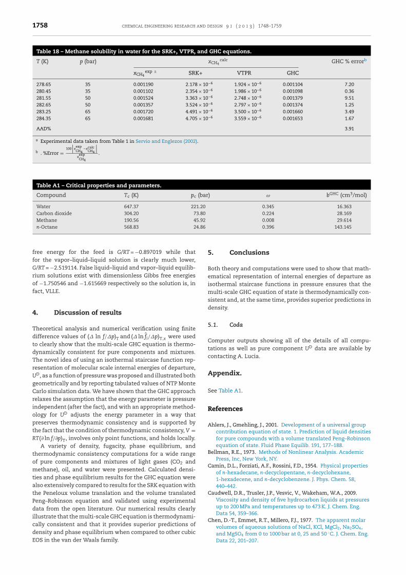
.2.2.1. Methane–Water VLE. Here we compare vapor–liquidhase equilibrium (VLE) results for the SRK+, VTPR, and GHCquations in the form of solubility of methane in liquid waterith experimental data taken from Servio and Englezos (2002)
or conditions that admit a VLE solution. Methane compo-ition in the equilibrium water-rich liquid phase is given inable 18.
While there is some scatter in the GHC predictions ofethane solubility in water shown in Table 18, overall these
esults are quite reasonable and capture all of the correcthysics associated with gas solubility. In particular, the multi-cale GHC equation predicts decreasing methane solubilitydegassing) with increasing temperature and higher methaneolubility with increasing pressure. Remember, unlike many
ther EOS, the multi-scale GHC equation does not use binary
nteraction parameters (kijs) and is purely predictive. In
Table 17 – Some mixture density results for SRK+, VTPR, ePSRK
Mixture Nd AAD%SRK+ VTPR PS
CO2–H2O 24 2.30 1.38 4NaCl–H2O 68 NA NA NA
.47 1.27 0.75
contrast, calculated methane solubility in water using theSRK+ equation with no binary interaction parameter (i.e.,kij = 0) and the VTPR equation at the conditions given inTable 18 are quite poor – 3 orders of magnitude too low.
3.2.2.2. CO2–Octane–Water VLLE. The purpose of this exam-ple is to show that the multi-scale GHC equation is capableof reliably predicting 3-phase equilibrium. Therefore, con-sider again a mixture of 30 mol% CO2, 20 mol% n-octane and50 mol% water at 313.15 K and 20 bar. Table 10 gives the feedand VLLE solution. Pure component critical properties and bparameters for the GHC equation can be found in Appendix.
In this example, the VLLE solution is found by travers-ing a sequence of flash sub-problems – in this case from
single liquid to liquid–liquid, to vapor–liquid, and finallyto vapor–liquid–liquid equilibrium. The dimensionless Gibbs
, and GHC equations.
error ReferenceRK ePSRK GHC
.03 NA 0.67 Teng et al. (1997) 2.65 0.91 Chen et al. (1977)
1758 chemical engineering research and design 9 1 ( 2 0 1 3 ) 1748–1759
Table 18 – Methane solubility in water for the SRK+, VTPR, and GHC equations.
free energy for the feed is G/RT = −0.897019 while thatfor the vapor–liquid–liquid solution is clearly much lower,G/RT = −2.519114. False liquid–liquid and vapor–liquid equilib-rium solutions exist with dimensionless Gibbs free energiesof −1.750546 and −1.615669 respectively so the solution is, infact, VLLE.
4. Discussion of results
Theoretical analysis and numerical verification using finitedifference values of (� ln f/�p)T and (� ln fi/�p)T,x were usedto clearly show that the multi-scale GHC equation is thermo-dynamically consistent for pure components and mixtures.The novel idea of using an isothermal staircase function rep-resentation of molecular scale internal energies of departure,UD, as a function of pressure was proposed and illustrated bothgeometrically and by reporting tabulated values of NTP MonteCarlo simulation data. We have shown that the GHC approachrelaxes the assumption that the energy parameter is pressureindependent (after the fact), and with an appropriate method-ology for UD adjusts the energy parameter in a way thatpreserves thermodynamic consistency and is supported bythe fact that the condition of thermodynamic consistency, V =RT(∂ ln f/∂p)T, involves only point functions, and holds locally.
A variety of density, fugacity, phase equilibrium, andthermodynamic consistency computations for a wide rangeof pure components and mixtures of light gases (CO2 andmethane), oil, and water were presented. Calculated densi-ties and phase equilibrium results for the GHC equation werealso extensively compared to results for the SRK equation withthe Peneloux volume translation and the volume translatedPeng–Robinson equation and validated using experimentaldata from the open literature. Our numerical results clearlyillustrate that the multi-scale GHC equation is thermodynami-cally consistent and that it provides superior predictions of
density and phase equilibrium when compared to other cubicEOS in the van der Waals family.
5. Conclusions
Both theory and computations were used to show that math-ematical representation of internal energies of departure asisothermal staircase functions in pressure ensures that themulti-scale GHC equation of state is thermodynamically con-sistent and, at the same time, provides superior predictions indensity.
5.1. Coda
Computer outputs showing all of the details of all compu-tations as well as pure component UD data are available bycontacting A. Lucia.
Appendix.
See Table A1.
References
Ahlers, J., Gmehling, J., 2001. Development of a universal groupcontribution equation of state. 1. Prediction of liquid densitiesfor pure compounds with a volume translated Peng–Robinsonequation of state. Fluid Phase Equilib. 191, 177–188.
Bellman, R.E., 1973. Methods of Nonlinear Analysis. AcademicPress, Inc, New York, NY.
Camin, D.L., Forziati, A.F., Rossini, F.D., 1954. Physical propertiesof n-hexadecane, n-decyclopentane, n-decyclohexane,1-hexadecene, and n-decyclobenzene. J. Phys. Chem. 58,440–442.
Caudwell, D.R., Trusler, J.P., Vesvic, V., Wakeham, W.A., 2009.Viscosity and density of five hydrocarbon liquids at pressuresup to 200 MPa and temperatures up to 473 K. J. Chem. Eng.Data 54, 359–366.
Chen, D.-T., Emmet, R.T., Millero, F.J., 1977. The apparent molarvolumes of aqueous solutions of NaCl, KCl, MgCl2, Na2SO4,
and MgSO4 from 0 to 1000 bar at 0, 25 and 50 ◦C. J. Chem. Eng.Data 22, 201–207.
chemical engineering research and design 9 1 ( 2 0 1 3 ) 1748–1759 1759
D
G
K
K
K
L
L
L
L
M
M
ysthe, D.K., Fuchs, A.H., Rousseau, B., 2000. Fluid transportproperties by equilibrium molecular dynamics, III. Evaluationof united atom interaction potential models of pure alkanes. J.Chem. Phys. 112, 7581–7590.
oldon, A., Dabrowska, K., Hofman, T., 2007. Densities andexcess volumes of the 1,3-dimethylimidazoliummethylsulfate + methanol system from (313.15 to 33.15) K andpressures from (0.1 to 25) MPa. J. Chem. Eng. Data 52,1830–1837.
ell, G.S., Whalley, E., 1965. The PVT properties of water, I. Liquidwater in the temperature range 0 to 150 degrees C and atpressures up to 1 kb. Philos. Trans. Roy. Soc. Lond. A 258,565–614 (1094).
essel’man, P.M., et al., 1970. Transactions of the 3rd all-unionconference on thermophysics. In: Thermophysical Propertiesof Gases. Nauka Press, Moscow.
iepe, J., Horstmann, S., Fischer, K., Gmehling, J., 2004.Application of the PSRK model for systems containing strongelectrolytes. Ind. Eng. Chem. Res. 43, 6607–6615.
iu, K., Wu, Y., McHugh, M.A., Baled, H., Enick, R.M., Morreale,B.D., 2010. Equation of state modeling of high-pressure,high-temperature hydrocarbon density data. J. Supercrit.Fluids 55, 701–711.
ucia, A., 2010. A multi-scale Gibbs–Helmholtz constrained cubicequation of state. J. Thermodyn., article id: 238365.
ucia, A., Bonk, B.M., Waterman, R.R., Roy, A., 2012. A multi-scaleframework for multi-phase equilibrium flash. Comput. Chem.Eng. 36, 79–98.
ucia, A., Bonk, B.M., 2012. Molecular geometry effects and theGibbs–Helmholtz constrained equation of state. Comput.Chem. Eng. 37, 1–14.
agee, J.W., Bruno, T.J., 1996. Isochoric (p, �, T) measurements forliquid toluene from 180 K to 400 K at pressures to 35 MPa. J.Chem. Eng. Data 41, 900–905.
agee, J.W., Ely, J.F., 1986. Specific heats of saturated and
compressed liquid and vapor carbon dioxide. Int. J.Thermophys. 7, 1163–1182.
Mora’vkova’, L., Wagner, Z., Aim, K., Linek, J., 2006. (P, Vm, T)measurements of (octane + 1-chlorohexane) at temperaturesfrom 298. 15 K to 328. 15 K and at pressures up to 40 MPa. J.Chem. Thermodyn. 38, 861–870.
Peneloux, A., Rauzy, E., Freze, R., 1982. A consistent correction forRedlich–Kwong–Soave volumes. Fluid Phase Equilib. 8,7–23.
Peters, C.J., van der Kooi, H.J., De Swaan Arons, J., 1987.Measurements and calculations of phase equilibria for(ethane + tetracosane) and (p, Vm, T) of liquid tetracosane. J.Chem. Thermodyn. 19, 395–405.
Servio, P., Englezos, P., 2002. Measurement of dissolved methanein water in equilibrium with its hydrate. J. Chem. Eng. Data 47,87–90.
Soave, G., 1972. Equilibrium constants from a modifiedRedlich–Kwong equation of state. Chem. Eng. Sci. 27,1197–1203.
Templin, P.R., 1956. Coefficient of volume expansion forpetroleum waxes and pure n-paraffins. Ind. Eng. Chem. 48,154–161.
Teng, H., Yamasaki, A., Chun, M.-K., Lee, H., 1997. Solubility ofliquid CO2 in water at temperatures from 278 K to 293 K from6.44 MPa to 29.49 MPa and densities of the correspondingaqueous phase. J. Chem. Thermodyn. 29,1301–1310.
van Hook, A., Silver, L., 1942. Pre-melting anomalies of somelong-chain normal paraffin hydrocarbons. J. Chem. Phys. 10,686–690.
Vargaftik, N.B., 1983. Handbook of Physical Properties of Liquidsand Gases: Pure Substances and Mixtures, 2nd ed.Hemisphere, Bristol, UK.
Walas, S.M., 1985. Phase Equilibria in Chemical Engineering.Butterworth Publishers, Stoneham, MA.