doi.org/10.26434/chemrxiv.12960197.v1

Thermodynamic Discrimination Between Energy Sources for ChemicalReactionsZachary Schiffer, Aditya Limaye, Karthish Manthiram

Submitted date: 16/09/2020 • Posted date: 17/09/2020Licence: CC BY-NC-ND 4.0Citation information: Schiffer, Zachary; Limaye, Aditya; Manthiram, Karthish (2020): ThermodynamicDiscrimination Between Energy Sources for Chemical Reactions. ChemRxiv. Preprint.https://doi.org/10.26434/chemrxiv.12960197.v1

Chemical transformations traverse large energy differences, yet the choice of energy source to drive achemical reaction is often decided on a case-by-case basis; there is no fundamentally-driven, universalframework with which to analyze and compare the choice of energy source for chemical reactions. In thiswork, we present a reaction-independent expression for the equilibrium constant as a function of temperature,pressure, and voltage. With a specific set of axes, all reactions can be represented by a single (x,y) point anda quantitative divide between electrochemically and thermochemically driven reactions is visually evident. Inaddition, we show that our expression has a strong physical basis in work and energy fluxes to the system,although more specific data about reaction operation is necessary to provide a quantitative energy analysis.Overall, this universal equation and facile visualization of chemical reactions enables quick and informedjustification for electrochemical versus thermochemical energy sources without knowledge of detailed processparameters.

File list (2)

download fileview on ChemRxivManuscript.pdf (1.91 MiB)

download fileview on ChemRxivSI.pdf (1.36 MiB)

Thermodynamic Discrimination between Energy Sources for ChemicalReactions

Zachary J Schiffera, Aditya M. Limayea, Karthish Manthirama,∗

aDepartment of Chemical Engineering, Massachusetts Institute of Technology, Cambridge, Massachusetts 02139, UnitedStates

Abstract

Chemical transformations traverse large energy differences, yet the choice of energy source to drive a chemicalreaction is often decided on a case-by-case basis; there is no fundamentally-driven, universal framework withwhich to analyze and compare the choice of energy source for chemical reactions. In this work, we presenta reaction-independent expression for the equilibrium constant as a function of temperature, pressure, andvoltage. With a specific set of axes, all reactions can be represented by a single (x, y) point and a quantitativedivide between electrochemically and thermochemically driven reactions is visually evident. In addition, weshow that our expression has a strong physical basis in work and energy fluxes to the system, although morespecific data about reaction operation is necessary to provide a quantitative energy analysis. Overall, thisuniversal equation and facile visualization of chemical reactions enables quick and informed justification forelectrochemical versus thermochemical energy sources without knowledge of detailed process parameters.

Keywords: Electrochemistry, Chemical thermodynamics, Electrochemical synthesis

In chemical synthesis, the making and breakingof chemical bonds often requires traversing largeenergy differences. In fact, the basic chemical in-dustry accounts for close to 20% of total deliveredenergy consumption in the industrial sector, which5

itself uses the most delivered energy of any end-usesector globally (54%) [1, 2]. Traditionally, indus-trial chemical synthesis has relied on pressure andtemperature as driving forces to synthesize chem-icals; a reactor requires an exchange of heat and10

work in order to drive a chemical transformation[3, 2, 4]. Yet, with the advent of abundant andaccessible renewable electricity, it is attractive toconsider driving chemical reactions that are conven-tionally driven with temperature and pressure with15

electrical voltage instead [5, 6, 7, 8, 9]. Hence, one isconfronted with the question, “why should a givenchemical reaction be driven preferentially with tem-perature (thermal energy), pressure (mechanicalenergy), or voltage (electrical energy)?” The re-20

sponse to this question is generally either broad andqualitative or extremely reaction-specific. Broadly,

∗To whom correspondence should be addressed. E-mail:karthish@mit.edu

if a reaction is highly endothermic (results in a verypositive change in enthalpy), then one may preferan electrochemical approach that avoids excessively25

high operating temperatures to shift the equilib-rium toward products [10, 9]. Additionally, if a re-action requires high pressures to drive conversion toproducts via Le Chatelier’s principle, then one mayprefer using voltage to avoid these excessively high30

pressures. Technoeconomic analyses are also oftenused to discriminate between thermochemical andelectrochemical driving forces based on feedstockcosts and system efficiencies [11, 12, 13, 14, 15, 16].However, these technoeconomic analyses remain fo-35

cused on specific reactions without investigating thephysical basis for the preference of driving force ina general manner. While many of the choices inthe driving chemical reactions are determined byfactors such as kinetics, cost, and safety, research40

and development often begins before estimates ofthese specific parameters are known. Accordingly,an intermediate-level heuristic for choosing a driv-ing force based on available physical parameters ismissing; specifically, one that is simple and intu-45

itive, yet also quantitative and dependable across awide range of chemical reactions.

Preprint submitted to ChemRxiv September 16, 2020

We address the question of how to discriminatebetween energy sources for driving chemical reac-tions via a theoretical framework built around re-50

action thermodynamics. Efficiency and thermo-dynamic limits on extraction of useful work havebeen studied for centuries (e.g., with the Carnotengine) [17, 18], and more recent work has slowlyrelaxed ideal constraints to add in real-world prac-55

ticalities via developments in fields such as endore-versible thermodynamics and finite-time thermody-namics [19, 20]. However, these theories are of-ten built to describe the extraction of energy froma chemical reaction, e.g., in a combustion engine,60

and they often still require significant knowledgeof specific process parameters such as heat trans-fer coefficients, compressor efficiencies, thermody-namic paths, etc [21]. In this work, we constructa universal equation to describe and analyze the65

thermodynamics of chemical reactions driven bytemperature, pressure, and voltage. We have fo-cused on these driving forces due to their preva-lence in chemical synthesis, although the analysiscan be extended to the direct use of photons or70

mechanochemical methods. We compare heat, me-chanical work, and electrical work as energy inputsto a chemical system and find that an ideal, loss-less model of energy comparison provides a phys-ical basis for our non-dimensional thermodynamic75

parameter analysis. After constructing a universalequation, we then introduce a facile visualizationmethod for comparing chemical reactions, with afocus on redox reactions (voltage is generally notan option for non-redox reactions), and show a80

clear divide between chemical reactions tradition-ally driven by elevated temperatures and pressuresin industry and reactions that rely on electrical volt-age. Our approach provides a simple, universalmethod to justify using temperature, pressure, or85

voltage as a driving force for a chemical reaction,and our analysis can be leveraged by researchers ina broad range of fields to help determine the impor-tant systems-level choice of thermodynamic drivingforce.90

Results and discussion

Non-dimensionalization of reaction equilibrium

We are interested in comparing the effects of tem-perature, pressure, and voltage as driving forces forshifting the equilibrium of a chemical reaction. Ac-95

cordingly, we start with a chemical reaction that

has some defined stoichiometry given by,∑i

νiAi = 0, (1)

where νi are the stoichiometric coefficients forchemical species Ai. Chemical equilibrium at con-stant temperature (T ), pressure (P ), and voltage100

(E) provides the constraint,∑i

νiµi(T, P,E) = 0, (2)

where µi are the species chemical potentials. As-suming that the system is an ideal mixture of gasesand that ∆CP,rxn ≡

∑i νiCP,i = 0, the equilibrium

constant, K, is a simple function of thermodynamic105

variables (Supplemental Derivation S1) [22, 23, 24],

logeK =−∆Grxn(T, P,E)

RT(3)

= −∆H0rxn

RT− ne−FE

RT−∆nrxn loge

P

P 0

+∆S0

rxn

R,

where ∆H0rxn and ∆S0

rxn are the enthalpy and en-tropy of reaction, respectively, at ambient con-ditions (namely no applied voltage, T = T 0 =298.15 K, and P = P 0 = 1 bar), R is the ideal gas110

constant, ne− is the minimum number of electronsnecessarily transferred in the overall reaction (Sup-plemental Derivation S1), and ∆nrxn ≡

∑i∈gas νi.

Although we assume for simplicity that all of ourcomponents are gases (with a few exceptions for115

pure liquids and solids), the extension to liquids,dissolved species, and solids is not difficult to incor-porate when going through the full derivation (Sup-plemental Derivation S1). Equation 3 is a famil-iar description of the equilibrium constant with one120

major difference: we have defined K ≡∏i∈gas y

νii ,

with yi being the mole fraction of each componentin the gas phase, instead of the more traditionalK =

∏i pνii , where pi is the partial pressure of

a species (i.e., the activity of an ideal gas) [25].125

In this work, the equilibrium constant is definedby equation 3 instead of the traditional definitionso that pressure will be explicitly included in theexpression. Through equation 3 and proper sto-ichiometry normalization, we can better compare130

reaction equilibriums based on a more consistentrelationship between mole fractions and K that is

2

not present when K is written in terms of activity(e.g., partial pressures) instead of mole fractions.

The practically relevant quantity for describing a135

chemical reaction is conversion, not the equilibriumconstant. However, conversion will be dependenton the exact reaction equation and not a universalfunction. To keep the analysis general, the equi-librium constant, K, will be used as a proxy for140

conversion since conversion is a strictly increasing,sigmoidal function of K ranging from 0 to 1 (Sup-plemental Derivation S2).

Unfortunately, the expression for the equilib-rium constant given by equation 3 does not al-145

low for facile comparison of temperature, pressure,and voltage in its current form since the quanti-ties ∆H0

rxn, ∆S0rxn, ∆nrxn, and ne− are reaction-

specific, preventing a general analysis of chemi-cal reaction equilibrium. To facilitate a compar-150

ison, the equilibrium constant expression can benon-dimensionalized to remove any specifics aboutthe chemical reaction. Non-dimensionalization isa useful tool for solving differential equations incertain limits and for quickly determining charac-155

teristic properties of a system such as time andlength; for these reasons it finds wide use acrossthe fields of chemical engineering, physics, fluid dy-namics, etc [26]. In the case of a chemical reac-tion, non-dimensionalization combines the reaction-160

specific details of the system with the reactionoperating conditions to create new variables thatare reaction-independent and scale simply with thethermodynamic driving forces of interest (Figure1, Supplemental Derivation S3). Traditional non-165

dimensionalization, e.g., of reaction-diffusion sys-tems, relies on the structure of a differential equa-tion to provide the non-dimensional groupings; analgebraic equation such as equation 3 does nothave equivalently straightforward non-dimensional170

groupings, and non-dimensionalization must in-stead rely on underlying physical intuition.

Equation 3 can be non-dimensionalized toachieve a universal expression for how thermal, me-chanical, and electrical energy shift the chemical175

equilibrium through non-dimensional temperature(T → Θ), pressure (P → Π), and voltage (E → Ψ),

Figure 1: Non-dimensionalization scheme for thermody-namic variables. Given a generic reaction, here shown asthe conversion of reactants A and B to products C and D,reaction-specific thermodynamic parameters (right) and thereaction operation conditions (left) can be combined to ob-tain non-dimensional groupings that scale with the thermo-dynamic driving forces and enable non-dimensionalization ofequation 3 to obtain equation 4.

Θ ≡ RT loge 10

∆H0rxn

,

Π ≡ ∆nrxn log10

P

P 0,

Ψ ≡ ne−FE

∆H0rxn

,

σ ≡ ∆Srxn

R loge 10,

log10K = − 1

Θ− Ψ

Θ−Π + σ. (4)

Note that we have chosen to use Θ ∝ T insteadof a potentially “natural” quantity Θ ∝ 1/T so thatchanges in Θ are more intuitively interpretable [27] .180

One of the advantages of equation 4 is that all reac-tions collapse onto simple plots that show the equi-librium constant, a proxy for reaction conversion, asa function of non-dimensional thermodynamic driv-ing forces (Figure 2). This visualization reveals that185

crossing equilibrium contours with pressure requiresa larger relative increase in thermodynamic drivingforce than crossing equilibrium contours with tem-perature or voltage (further supporting analysis ofcontours and derivatives provided in Supplemental190

Derivation S4). This discrepancy is magnified bythe fact that the scaling of Π is logarithmic withpressure whereas the scalings of Θ and Ψ are linearwith temperature and voltage, respectively.

So far, the analysis has relied on the math-195

ematical form of our non-dimensional parame-

3

Figure 2: Plots of equation 4. Every chemical reaction can be mapped onto these universal plots. When no voltage is applied(Ψ = 0), contours showing how pressure and temperature affect reaction equilibrium are visualized (a). At ambient pressure(Π = 0), contours showing how voltage and temperature affect the reaction equilibrium are visualized (b). Contours of howvoltage and pressure affect the equilibrium at 298.15 K (ambient temperature) are not as simple to visualize; there is a Θambient

term in these contours that make the plot less useful because it is reaction dependent and not generalizable (these plots and fulldiscussion in Supplemental Derivation S4). Crossing the constant K contours using pressure requires a larger relative change innon-dimensional driving force than it does using voltage or temperature. Note that the colorbar axis is log10K−σ so that theplot remains independent of reaction; different reactions will essentially provide a constant shift from σ that does not changethe shape of the plot. Additionally, that crossing Θ = 0 for a given reaction is impossible since the sign of Θ is determined bythe reaction enthalpy (a fixed quantity assuming ∆CP,rxn = 0).

ters. In practice, there are many alternative non-dimensional groupings with additional constant fac-tors or functional forms that would change thisanalysis. However, these non-dimensional ther-200

modynamic parameters (Figure 1) are not onlyconvenient from a mathematical perspective, butalso represent physical groupings related to analo-gous work and energy fluxes, discussed below, suchthat conclusions drawn from analysis of the non-205

dimensional thermodynamic parameters are physi-cally relevant.

Work and energy exchange

A direct comparison between temperature, pres-sure, and voltage is difficult since each driving force210

has different units. Even with our non-dimensionalscalings, there is no reason to assume a priorithat these non-dimensional parameters have anyphysical meaning and can be directly comparedto each other. Instead, a metric for comparing215

driving forces on equal footing would be to com-pare work and energy exchanges of the system; thiscomparison will provide a physical basis for ournon-dimensional parameters so that we can directlycompare them.220

In practice, no general method to convert be-tween thermodynamic parameters and work existssince heat and work are path functions. However,if the system does not have any energy losses, theoverall, steady-state energy exchanges of the system225

must obey the law of energy conservation,

WM +WE +Q = ∆H0rxn · z, (5)

where z is the reaction conversion at equilibrium,a function of K and defined between 0 and 1. Amore convenient form of equation 5 results fromnon-dimensionalization of the work terms with the230

reaction enthalpy as the characteristic energy of thesystem (Supplemental Derivation S5),

ΩWM + ΩWE + ΩQ = z. (6)

Ignoring the exact functional form of the workterms for now and assuming that the system isdriven by either pressure or voltage individually,235

but not both simultaneously, the constraint im-posed by equation 6 has the geometric form of aplane in ΩWi

–ΩQ space (Figure 3). Accordingly,for a system with no energy losses, any energy in-put will result in an equivalent change in conver-240

sion, regardless of the energy source. If additional

4

Figure 3: Conversion, z, as a function of various energy in-puts assuming no energy losses in the system. In this system,either pressure or voltage is utilized, but not both simultane-ously. In the absence of losses, all energy exchanges producethe same change in conversion, regardless of the source ofthe energy. Thus, in the absence of additional, reaction-and process-specific information, this energy analysis simplyprovides a physical basis for the non-dimensional analysis,as discussed in the main text.

information is available, such as the cost of electric-ity, efficiency of heat flux, compressor losses, etc.,there are a multitude of thermodynamic and tech-noeconomic heuristics that can lead to a quantita-245

tive conclusion, but these are beyond the scope ofthis work.

In the absence of more information, there arestill important insights to glean from the functionalforms of the work and heat inputs. In addition to250

the previous assumptions (ideal gas mixture and∆CP,rxn = 0), additional assumptions are necessaryto convert from thermodynamic parameters to workand energy fluxes: (1) the reactor is isothermal, iso-baric, and does not exchange mechanical work with255

the environment, and (2) the processes that bringthe inputs to the operating conditions and bringthe outputs back to ambient conditions have accessto a single heat bath at some Tbath. Given theseassumptions, as well as assuming unit efficiency of260

every process, the total energy and work exchangeswith the overall system are functions of the pre-vious thermodynamic parameters, the conversion,z = z(K), which is a function of the equilibriumconstant, and the single non-dimensional thermal265

bath temperature, Θbath ≡ RTbath loge 10∆H0

rxn(Supple-

mental Derivation S5) [28, 29, 30, 31],

ΩWE= −z(K)Ψ

ΩWM= −z(K)ΘbathΠ (7)

ΩQ = z(K) (Ψ + ΘbathΠ + 1)

Without additional practical information, our en-ergy analysis is qualitative, and these equations bythemselves do not reveal a preference for mechan-270

ical work, electrical work, or heat. However, theseequations do provide justification for our previousanalysis. We initially began our reaction analy-sis by non-dimensionalizing temperature, pressure,and voltage to remove any reaction-specific quanti-275

ties from the equilibrium expression given in equa-tion 3. The non-dimensionalization was intuitiveyet somewhat arbitrary, and there was no indica-tion that the non-dimensional parameters (Θ, Π,and Ψ) had any physical meaning. The energy280

analysis presented here, however, reveals that thenon-dimensional electrical work (ΩWE

) will scale di-rectly with non-dimensional voltage (Ψ), the non-dimensional mechanical work (ΩWM

) will scale di-rectly with non-dimensional pressure (Π), and the285

heat flux is a convolution of all the energy in-puts but has a clear characteristic energy given by∆H0

rxn, which was used to non-dimensionalize tem-perature (Θ). Accordingly, although the previousanalysis dealt with non-dimensional driving forces290

that were not, a priori, comparable, this energyanalysis reveals that these non-dimensional quanti-ties are reasonable proxies for work and energy ex-changes and that our non-dimensional analysis hasa strong physical basis. Direct comparisons of the295

non-dimensional thermodynamic parameters there-fore correspond to comparisons of analogous energyand work exchanges, validating conclusions drawnfrom such direct comparisons.

Example chemical reactions on universal plot300

While the universal colormaps of equation 4 areinteresting on their own (Figure 2), contour linesof constant K for a specific reaction help visual-ize the thermodynamics of that reaction. This isthe advantage of plotting the equilibrium constant305

in non-dimensional space: instead of qualitativelylooking at endo- vs. exo-thermicity or analyzinga specific reaction’s equilibrium constant at vari-ous temperatures, pressures and voltages, we canquantitatively display the influence of these driving310

5

forces on a single set of axes since the thermody-namic landscapes for individual reactions all col-lapse onto a single plot in non-dimensional space(Figure 2). Two well-studied reactions are ammo-nia synthesis (Reaction R1, industrially known as315

the Haber-Bosch process),

1

2N2 +

3

2H2 −−→ NH3 , (R1)

and water splitting (Reaction R2),

H2O −−→ H2 +1

2O2 . (R2)

The constant K contours for these reactions canbe plotted on the universal colormaps and com-pared (Figure 4) [32]. Using the reaction thermo-dynamic properties, dimensional parameters (T , P ,320

and E) are shown for each reaction on the sec-ondary axes. In addition to helping visualize theequilibrium constants for these reactions in stan-dard units, these secondary axes demonstrate thatthe non-dimensional axes span a sufficient range325

of operating conditions for most reactions. Thekey points to consider with these plots are: (1)the red dot represents ambient conditions, and thehorizontal distance to Θ = 0 is inversely propor-tional to the enthalpy of reaction; (2) the red verti-330

cal line attached to each ambient conditions pointon the pressure-temperature plots (Figure 4a andc) represents an increase of an order of magnitudein pressure; (3) the vertical distance from the reddot to the solid pink line (K = 1) on the voltage-335

temperature plots (Figure 4b and d) is the non-dimensional equilibrium potential of the reaction.

For the case of ammonia synthesis (Figure 4a andb), the thermodynamic equilibrium favors full con-version of nitrogen and hydrogen to ammonia at340

ambient conditions; however, kinetics mandate theuse of an elevated operating temperature and pres-sure. This reaction is an important example of theutility of thermodynamic analyses even for reac-tions where kinetics dictate operating conditions.345

The scaling of the axes (seen by the secondaryaxes) demonstrates that crossing equilibrium con-tours and moving around the thermodynamic equi-librium space with temperature and pressure arefeasible at practical operating conditions for am-350

monia synthesis. In other words, at a temperatureat which the kinetics are favorable for ammoniasynthesis, the visualization demonstrates that pres-sure can allow us to easily move through thermo-dynamic equilibrium space; this is reflected in the355

fact that ammonia synthesis is commercially prac-ticed at elevated pressures that enable higher equi-librium conversions. This is in contrast with watersplitting (Figure 4c and d), for which the visual-ization clearly demonstrates that increasing pres-360

sure decreases conversion, and enormous tempera-tures are necessary to achieve meaningful equilib-rium conversions. However, voltage remains a pow-erful tool, since approximately 1.2 V is sufficient todrive water splitting, a feasible amount compared to365

the high temperature or low pressure necessary oth-erwise. This analysis is currently limited to thermo-dynamic equilibrium considerations, while in realitytemperature, pressure, and voltage also play a rolein kinetics, cost, selectivity, and safety, all of which370

strongly influence the trade-offs between thermo-chemistry and electrochemistry. These other fac-tors are beyond the scope of this analysis as we aimto describe broad trends in driving forces for chem-ical reactions using a thermodynamic framework.375

Even without knowledge of these other factors, athermodynamic analysis reveals whether high con-version is even physically possible, a prerequisiteto engineering reactivity given operating conditionsdictated by kinetics and other non-thermodynamic380

constraints. This continues to motivate the searchfor catalysts that are active at lower temperaturesin the case of ammonia synthesis, while telling usnot to search for thermochemical water splittingcatalysts at ambient conditions due to thermody-385

namic restrictions.

While these universal colormaps are useful for vi-sualizing individual reactions, they are not idealfor comparing multiple reactions because they re-quire unique constant K contours for each reaction,390

meaning that multiple reactions would quickly ob-scure each other. Instead, the axes can be redefinedsuch that every reaction has the same K contours,facilitating direct comparison between different re-actions.395

Visual comparison and analysis of chemical reac-tions

Instead of using the non-dimensional groups de-rived above as axes, in which each reaction has adistinct set of K-contours, a simple variable trans-400

formation can collapse these to a single set of equi-librium K contours for all reactions (Figure 5).Specifically, the x-axis is transformed to 1/Θ andthe y-axis is transformed to Ψ/Θ + Π− σ (Supple-mental Derivation S6). In general, we assume that405

6

Figure 4: Plots of equation 4 for ammonia synthesis (Reaction R1) and water splitting (Reaction R2), using the given sto-ichiometry. Pink lines indicate constant K contours for each reaction, the red dots represent ambient conditions, and thevertical line extending from each red point in the thermochemistry plots (a and c) represents an increase in pressure of oneorder of magnitude. In particular, the horizontal distance from the red dot to Θ = 0 is inversely proportional to the enthalpyof reaction, and the vertical distance between the red dot and the solid pink line on the electrochemistry plots (b and d) repre-sents the non-dimensional equilibrium potential. Dimensional thermodynamic parameters on the secondary axes demonstratethat the axes span a sufficient range of operating conditions and are reaction dependent. Dimensional parameters also showhow reactions cannot cross Θ = 0 since that would correspond to a switch in sign of ∆H0

rxn, a quantity fixed by the reaction(assuming ∆CP,rxn = 0). Temperature and pressure enable facile movement in thermodynamic space for ammonia synthesis,whereas voltage is necessary to drive water splitting.

in addition to temperature, either voltage or pres-sure is being used to drive the reaction, not bothsimultaneously, which results in either Π = 0 orΨ = 0, respectively.

As depicted, in these axes a change in pressure or410

voltage corresponds to a vertical movement relativeto the reaction point and an increase (decrease) in Tcorresponds to a movement toward (away from) thepoint (0,Π − σ) (Figure 5a, Supplemental Deriva-tion S6). These new, composite axes allow for the415

direct comparison of chemical reactions since all re-actions have the same K contours, with each reac-tion at ambient conditions represented by a singlepoint,

(x, y)ambientrxn =

(1

Θambient,−σ

)(8)

=

(∆H0

rxn

RT 0 loge 10,− ∆S0

rxn

R loge 10

),

where T 0 = 298.15 K. For each reaction point at420

ambient conditions, the distance from the reactionpoint to x = 0 is proportional to ∆H0

rxn, the dis-tance to y = 0 is proportional to ∆S0

rxn, and thedistance to the solid black line (K = 1, given byy = −x) is proportional to the dimensional equi-425

librium potential of the reaction (Figure 5b, Sup-plemental Derivation S7).

7

Figure 5: Redefined axes such that all reactions have the same equilibrium K contours. A contour corresponding to K = 1 isindicated with a diagonal black line (y = −x). The filled red diamonds represent example reaction points at ambient conditionsgiven by equation 8. An increase in either pressure (Π) or voltage (Ψ) is a vertical movement on these axes (a, new reactionpoint given by blue square) and an increase in temperature (Θ) is a movement towards the point (0,Π − σ) (a, new reactionpoint given by blue circle, movement along the line connecting to the empty blue diamond). As shown, the x-coordinate ofeach point is proportional to ∆H0

rxn, the y-coordinate of each point is proportional to ∆S0rxn, and the vertical distance from

each point to the solid black line (K = 1, given by y = −x) is proportional to the dimensional equilibrium potential of thereaction (b). Further details in Supplemental Derivations S6 and S7.

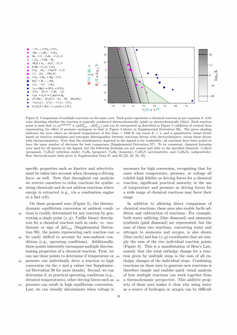
When multiple reactions are plotted on theseaxes, a clear divide appears between those that areconventionally driven thermochemically versus elec-430

trochemically (Figure 6). Reactions to the left ofthe K = 1 line (y = −x) are already thermodynam-ically favorable at ambient conditions. Any adjust-ment to the reaction conditions (e.g., an increasein temperature to improve kinetics) must keep the435

reaction as far left as possible to maintain thermo-dynamic favorability. If the reaction point is nearor to the right of the K = 1 line (y = −x), thenpressure or temperature can practically cross theequilibrium contours only if the reaction point is440

within a reasonable distance to the K = 1 line.In particular, to use pressure to drive conversion,the vertical distance from the reaction point to theline y = −x must be within a couple of orders ofmagnitude of pressure (a version of Figure 6 with445

pressure effects depicted for each reaction is shownin Supplemental Derivation S6).

If the reaction point lies to the right of theK = 1 line (y = −x), then the reaction can bedriven to quantifiable conversion using just tem-450

perature when the horizontal distance from thereaction point to y = −x is sufficiently smalland the reaction point does not lie in the top-right quadrant; in that quadrant, the ∆H0

rxn and∆S0

rxn conspire to make the K = 1 contour un-455

reachable with temperature. The horizontal dis-

tance to y = −x is quantified by the tempera-ture, T eq, when K(P = 1 bar, T = T eq) = 1,namely when T eq = ∆H0

rxn/∆S0rxn. Due to phys-

ical practicalities, the operating temperature must460

be within a factor of ca. 5 of the ambient temper-ature (∼ 1500 K). Mathematically, this translatesto T eq/T ambient = 1/

(σΘambient

)≤ 5. For a reac-

tion point given by (x, y)ambientrxn on these axes, the

reaction can practically be driven by temperature465

alone when 1/(σΘambient

)= −x/y ≤ 5, approxi-

mately (green shading on Figure 6).

Voltage, however, is particularly well suited todrive chemical reactions that are far from theK = 1line since even large values of Ψ/Θ generally cor-470

respond to voltages of order 1 V (SupplementalDerivation S4). Thus, this visualization quanti-tatively supports our intuition, namely that reac-tions with large, positive values of ∆H0

rxn (highlyendothermic) are generally better driven by volt-475

age. In particular, reactions which require large ex-cursions on these non-dimensional axes can gener-ally only be done electrochemically (Figure 6, bluepoints). Those requiring small excursions on theseaxes can generally be done either electrochemically480

or thermochemically, and these reactions often aredriven with temperature and pressure due to in-dustrial expertise and convenience (Figure 6, pinkpoints). For reactions that could be driven eitherthermochemically or electrochemically, reaction-485

8

Figure 6: Comparison of multiple reactions on the same axes. Each point represents a chemical reaction as per equation 8, withcolor denoting whether the reaction is typically conducted thermochemically (pink) or electrochemically (blue). Each reactionpoint is such that (x, y)ambient ∝ (∆H0

rxn,−∆S0rxn) and can be interpreted as described in Figure 5 (addition of vertical lines

representing the effect of pressure analogous to that in Figure 4 shown in Supplemental Derivation S6). The green shadingindicates the area where an elevated temperature of less than ∼ 1500 K can reach K = 1, and a quantitative visual dividebased on reaction enthalpies and entropies distringuishes between reactions driven with electrochemistry versus those drivenwith thermochemistry. Note that the stoichiometry depicted in the legend is for readability; all reactions have been scaled tohave the same number of electrons for best comparison (Supplemental Derivation S7). To be consistent, chemical formulaswere used for all species in the legend, but the following formulas are not unique and refer to the specified chemical: C3H6O(propanal), C2H4O (ethylene oxide), C3H6 (propene), C6H6 (benzene), C3H3N (acrylonitrile), and C6H8N2 (adiponitrile).Raw thermodynamic data given in Supplemental Data S1 and S2 [32, 33, 34, 35].

specific properties such as kinetics and selectivitymust be taken into account when choosing a drivingforce, as well. Note that throughout our analysiswe restrict ourselves to redox reactions for synthe-sizing chemicals and do not address reactions where490

energy is extracted (e.g., via a combustion engineor a fuel cell).

On these proposed axes (Figure 5), the thermo-dynamic equilibrium conversion at ambient condi-tions is readily determined for any reaction by gen-495

erating a single point (x, y). Unlike binary descrip-tors for a chemical reaction such as endo- vs. exo-thermic or sign of ∆Grxn (Supplemental Deriva-tion S8), the points representing each reaction canbe easily shifted to account for non-ambient con-500

ditions (e.g., operating conditions). Additionally,these points inherently encompass multiple discrim-inating properties of a chemical reaction. First, wecan use these points to determine if temperature orpressure can individually drive a reaction to high505

conversion via the x and y values (see Supplemen-tal Derivation S6 for more details). Second, we candetermine if, at practical operating conditions (e.g.,elevated temperatures), other driving forces such aspressure can result in high equilibrium conversion.510

Last, we can visually discriminate when voltage is

necessary for high conversion, recognizing that forcases where temperature, pressure, or voltage allexhibit high fidelity as driving forces for a chemicalreaction, significant practical maturity in the use515

of temperature and pressure as driving forces fora wide range of chemical reactions may favor theirusage.

In addition to allowing direct comparison ofchemical reactions, these axes also enable facile ad-520

dition and subtraction of reactions. For example,both water splitting (blue diamond) and ammoniasynthesis (pink diamond) are represented, but thesum of these two reactions, converting water andnitrogen to ammonia and oxygen, is also shown525

(blue circle) and has (x, y) coordinates that are sim-ply the sum of the two individual reaction points(Figure 6). This is a manifestation of Hess’s Law,namely that the total enthalpy change for a reac-tion given by multiple steps is the sum of all en-530

thalpy changes of the individual steps. Combiningreactions on these axes to generate new reactions istherefore simple and enables quick visual analysisof how multiple reactions can work together froma thermodynamic perspective. This additive prop-535

erty of these axes makes it clear why using wateras a source of hydrogen or oxygen can be difficult

9

with pressure and temperature but is feasible withvoltage as a driving force; since the water splittingpoint is so far from the vertical axis (very endother-540

mic), the specific reaction where we want to replacehydrogen or oxygen would need to be equally far onthe opposite side of x = 0 to be thermochemicallyfeasible using water as a reactant.

Conclusions545

Beginning with the question: “why shoulda given chemical reaction be driven preferen-tially with temperature (thermal energy), pres-sure (mechanical energy), or voltage (electrical en-ergy)?” we developed a non-dimensional, reaction-550

independent expression for chemical equilibrium asa function of thermodynamic driving forces. Wethen analyzed the thermodynamics for multiple in-dustrial and lab-scale chemical reactions that relyon different combinations of temperature, pressure,555

and voltage as driving forces and compared themvisually on the same axes, finding a clear discrimi-nation between electrochemically and thermochem-ically driven reactions. Converting from tempera-ture, pressure, and voltage to heat and work fluxes560

reveals that our analysis has a strong physical basisin work and energy exchanges.

The universal equation and facile visualization ofchemical reactions provide both a quantitative jus-tification for thermodynamic driving force as well565

as an intuitive platform for comparing multiple re-actions. However, chemical reaction conditions areoften dictated by more than just thermodynamicsand require knowledge of kinetics, selectivity, costs,and associated unit operations, such as those in-570

volved in separations. Other parameters such asreactant availability, the possibility of modular anddistributed manufacturing, and safety are also nec-essary considerations. Thus, the decision betweenusing traditional heat and mechanical work to drive575

a reaction versus using electricity in reality dependson much more than the thermodynamics. However,academic and industrial research on chemical reac-tions often begins long before estimates of practicaloperating parameters are available. Quantitative580

thermodynamic visualizations of the type presentedhere can allow for comparing candidate reactionsand driving forces at the early stages of developingnew reactions and processes, before a process is suf-ficiently mature to inform detailed technoeconomic585

and safety analyses.

Methods

Thermodynamic data was taken from NIST [32],the Dortmund Data Bank [33], Lange’s Handbookof Chemistry [34], and group additivity theory via590

RMG [35] depending on availability, with the mostrecent data point used if multiple data points wereprovided (raw data provided in Supplemental Ta-ble S1). Derivations for all analytical thermo-dynamic expressions shown in the main text are595

provided in the Supplemental Derivations S6 andS7. Starting with the expression for an equilib-rium constant (equation 3), we derived an expres-sion that explicitly included the dependence on spe-cific driving forces of interest (pressure, tempera-600

ture, and voltage). This expression was then non-dimensionalized in preparation for better compari-son and visualization. Energy and work exchangeswere calculated by conducting energy and entropybalances. Analysis and visualization of all data was605

performed using Python and matplotlib. Prior topublication, this code will be hosted on Zenodo andbe identifiable with a DOI URL.

Supplemental Information

Document S1: Supplemental derivations and610

supplemental tables S1-S2.

Acknowledgments

This material is based on work supported bythe National Science Foundation under grant no.1944007. The authors thank Nathan Corbin, Niki-615

far Lazouski, and Kindle Williams for useful discus-sions. ZJS and AML also acknowledge a graduateresearch fellowship from the National Science Foun-dation under Grant No. 1745302.

Author Contributions620

Conceptualization, Z.J.S., and K.M.; Methodol-ogy, Z.J.S., A.M.L., and K.M.; Software, Z.J.S.;Validation, Z.J.S., A.M.L., and K.M.L.; Investiga-tion, Z.J.S., A.M.L, and K.M.; Resources, Z.J.S.,A.M.L., and K.M.; Writing—Original Draft, Z.J.S.;625

Writing—Review &Editing, Z.J.S., A.M.L, andK.M.; Visualization, Z.J.S.; Supervision, K.M.;Funding Acquisition, K.M.

10

Declaration of Interests

The authors declare no competing interests.630

References

[1] EIA, International Energy Outlook 2016, Tech. rep.(2016).

[2] IEA, ICCA, DECHEMA, Technology Roadmap: En-ergy and GHG Reductions in the Chemical Industry635

via Catalytic Processes, Tech. rep. (2013).[3] C. M. Friend, B. Xu, Heterogeneous Catalysis:

A Central Science for a Sustainable Future, Ac-counts of Chemical Research 50 (3) (2017) 517–521.doi:10.1021/acs.accounts.6b00510.640

URL http://pubs.acs.org/doi/abs/10.1021/acs.

accounts.6b00510

[4] A. Arora, A. Gambardella, Implications for Energy In-novation from the Chemical Industry, in: Accelerat-ing Energy Innovation: Insights from Multiple Sec-645

tors, University of Chicago Press, 2011, pp. 87–111.doi:10.7208/chicago/9780226326856.001.0001.URL http://www.nber.org/chapters/c11751

[5] K. M. van Geem, V. V. Galvita, G. B. Marin, Mak-ing chemicals with electricity, Science 364 (6442) (2019)650

734–735. doi:10.1126/science.aax5179.[6] S. Gu, B. Xu, Y. Yan, Electrochemical Energy Engi-

neering: A New Frontier of Chemical Engineering In-novation, Annual Review of Chemical and Biomolec-ular Engineering 5 (1) (2014) 429–454. doi:10.1146/655

annurev-chembioeng-060713-040114.[7] C. Schnuelle, J. Thoeming, T. Wassermann, P. Thier,

A. v. Gleich, S. Goessling-Reisemann, Socio-technical-economic assessment of power-to-X: Potentials and lim-itations for an integration into the German energy sys-660

tem, Energy Research & Social Science 51 (2019) 187–197.

[8] Z. J. Schiffer, K. Manthiram, Electrification and Decar-bonization of the Chemical Industry, Joule 1 (1) (2017)10–14. doi:10.1016/j.joule.2017.07.008.665

URL http://dx.doi.org/10.1016/j.joule.2017.07.

008

[9] G. G. Botte, Electrochemical Manufacturing in theChemical Industry, Interface magazine 23 (3) (2014)49–55. doi:10.1149/2.F04143if.670

URL http://interface.ecsdl.org/cgi/doi/10.1149/

2.F04143if

[10] Z. Wang, R. R. Roberts, G. F. Naterer, K. S. Gabriel,Comparison of thermochemical, electrolytic, photoelec-trolytic and photochemical solar-to-hydrogen produc-675

tion technologies, International Journal of HydrogenEnergy 37 (21) (2012) 16287–16301. doi:10.1016/j.

ijhydene.2012.03.057.URL http://dx.doi.org/10.1016/j.ijhydene.2012.

03.057680

[11] M. Jouny, W. Luc, F. Jiao, General Techno-EconomicAnalysis of CO2 Electrolysis Systems, Industrial andEngineering Chemistry Research 57 (6) (2018) 2165–2177. doi:10.1021/acs.iecr.7b03514.

[12] Y. Zhao, B. P. Setzler, J. Wang, J. Nash, T. Wang,685

B. Xu, Y. Yan, An Efficient Direct Ammonia Fuel Cellfor Affordable Carbon-Neutral Transportation, Joule(2019) 1–13doi:10.1016/j.joule.2019.07.005.

URL https://linkinghub.elsevier.com/retrieve/

pii/S2542435119303216690

[13] J. Na, B. Seo, J. Kim, C. W. Lee, H. Lee, Y. J.Hwang, B. K. Min, D. K. Lee, H. S. Oh, U. Lee,General technoeconomic analysis for electrochemicalcoproduction coupling carbon dioxide reduction withorganic oxidation, Nature Communications 10 (1)695

(2019). doi:10.1038/s41467-019-12744-y.URL http://dx.doi.org/10.1038/

s41467-019-12744-y

[14] K. Muller, K. Brooks, T. Autrey, Hydrogen Storage inFormic Acid: A Comparison of Process Options, En-700

ergy Fuels 31 (2017) 12603–12611. doi:10.1021/acs.

energyfuels.7b02997.[15] M. Jouny, G. S. Hutchings, F. Jiao, Carbon monoxide

electroreduction as an emerging platform for carbonutilization, Nature Catalysis 2 (12) (2019) 1062–1070.705

doi:10.1038/s41929-019-0388-2.URL http://dx.doi.org/10.1038/

s41929-019-0388-2

[16] S. Verma, S. Lu, P. J. Kenis, Co-electrolysis of CO2and glycerol as a pathway to carbon chemicals with710

improved technoeconomics due to low electricityconsumption, Nature Energy 4 (6) (2019) 466–474.doi:10.1038/s41560-019-0374-6.URL http://dx.doi.org/10.1038/

s41560-019-0374-6715

[17] S. Carnot, Reflexions sur la puissance motrice du feu etsur les machines propres a developper cette puissance,Paris, 1824.

[18] J. Smeaton, XVIII. An experimental enquiry concern-ing the natural powers of water and wind to turn720

mils, and other machines, depending on a circular mo-tion., Philosophical Transactions of the Royal Society51 (1759) 100–174.

[19] K. H. Hoffmann, An Introduction to Endore-versible Thermodynamics (2008) 1–18doi:10.1478/725

C1S0801011.[20] B. Andresen, R. S. Berry, A. Nitzan, P. Salamon, Ther-

modynamics in finite time. I. The step-Carnot cycle,Physical Review A 15 (5) (1977) 2086–2093. doi:

10.1103/PhysRevA.15.2086.730

[21] S. Sieniutycz, J. Jezowski, Energy limits for thermalengines and heat pumps at steady states, 2018. doi:

10.1016/b978-0-08-102557-4.00003-7.[22] G. Inzelt, Crossing the bridge between thermodynam-

ics and electrochemistry. From the potential of the cell735

reaction to the electrode potential, ChemTexts 1 (1)(2015) 1–11. doi:10.1007/s40828-014-0002-9.

[23] E. Keszei, Chemical Thermodynamics: An introduc-tion. doi:10.1017/CBO9781107415324.004.

[24] E. Clarke, D. Glew, Evaluation of Thermodynamic740

Functions from Equilibrium Constants, Transactions ofthe Faraday Society 62 (1966) 539–547.

[25] J. O. Bockris, Comprehensive Treatise of Electrochem-istry Vol. 3: Electrochemical Energy Conversion andStorage, 1981. doi:10.1007/978-1-4615-6687-8\_8.745

[26] T. Hecksher, Insights through dimensions, NaturePhysics 13 (10) (2017) 1026. doi:10.1038/nphys4285.

[27] J. Meixner, Coldness and temperature, Archive for Ra-tional Mechanics and Analysis 57 (3) (1975) 281–290.doi:10.1007/BF00280159.750

[28] N. M. Bazhin, Mechanism of electric energy produc-tion in galvanic and concentration cells, Journal of En-gineering Thermophysics 20 (3) (2011) 302–307. doi:

11

10.1134/S1810232811030076.[29] N. M. Bazhin, V. N. Parmon, Conversion of the chem-755

ical reaction energy into useful work in the Van’t Hoffequilibrium box, Journal of Chemical Education 84 (6)(2007) 1053–1055. doi:10.1021/ed084p1053.

[30] A. Kowalewicz, Fuel-cell: power for future, Journal ofKONES 8 (3) (2001) 325–333.760

[31] A. Z. Panagiotopoulos, Essential Thermodynamics, 1stEdition, CreateSpace Independent Publishing Plat-form, 2011.

[32] D. Burgess, Thermochemical Data, in: P. Linstrom,W. Mallard (Eds.), NIST Chemistry WebBook, NIST765

Standard Reference Database Number 69, NationalInstitute of Standards and Technology, Gaithersburg,MD, Ch. Thermochem. doi:10.18434/T4D303.

[33] Dortmund Data Bank (2020).URL www.ddbst.com770

[34] N. A. Lange, Lange’s Handbook of Chemistry, 15th Edi-tion, McGraw-Hill, Inc., 1999.

[35] C. W. Gao, J. W. Allen, W. H. Green, R. H. West,Reaction Mechanism Generator: Automatic construc-tion of chemical kinetic mechanisms, Computer Physics775

Communications 203 (2016) 212–225. doi:10.1016/j.

cpc.2016.02.013.URL http://dx.doi.org/10.1016/j.cpc.2016.02.013

12

download fileview on ChemRxivManuscript.pdf (1.91 MiB)

Supplemental Information for ThermodynamicDiscrimination between Energy Sources for Chemical

Reactions

Zachary J Schiffer1, Aditya M. Limaye1, and Karthish Manthiram1,*

1Department of Chemical Engineering, Massachusetts Institute of Technology,Cambridge, Massachusetts 02139, United States

*To whom correspondence should be addressed. E-mail: karthish@mit.edu

ContentsSupplemental Data S-1S1 Raw data for chemical species . . . . . . . . . . . . . . . . . . . . . . . . . . S-1S2 Raw reaction thermodynamics for reaction equations . . . . . . . . . . . . . S-2

Supplemental Derivations S-3S1 Equilibrium constant . . . . . . . . . . . . . . . . . . . . . . . . . . . . . . . S-3S2 Relationship between equilibrium constant K and conversion . . . . . . . . . S-5S3 Non-dimensionalization of equilibrium expression . . . . . . . . . . . . . . . S-6S4 Constant K contours and comparison of driving forces . . . . . . . . . . . . S-7S5 Derivation of work and energy exchange . . . . . . . . . . . . . . . . . . . . S-10S6 Redefinition of axes to collapse K contours . . . . . . . . . . . . . . . . . . . S-15S7 Scaling of reaction stoichiometry to compare reactions . . . . . . . . . . . . . S-16S8 Simple Descriptors . . . . . . . . . . . . . . . . . . . . . . . . . . . . . . . . S-18

Supplemental References S-20

Supplemental Data

S1 Raw data for chemical species

These raw values are used to generate the reaction enthalpies and entropies used in the maintext (primarily Figure 6).

S-1

Table S1: Molecule raw thermodynamic parameters

Molecule ∆H0f (kJ/mol) a S0

f (J/mol.K) a PhaseCO2 -393.52 213.79 gCO -110.53 197.66 gCH4 -74.6 186.25 gH2O -241.83 188.84 gH2O -285.83 69.95 `MeOH -205 239.81 c gH2 0 130.68 gN2 0 191.61 gO2 0 205.15 gNH3 -45.9 192.77 gAl2O3 -1675.69 50.92 sC b 0 5.6 sAl 0 28.3 s

NaCl -411.12 72.11 sCl2 0 223.08 g

NaOH -425.93 64.46 sPropanal -188.7 304.4 gC2H4 52.4 219.32 gC2H6 -84.0 229.1 d gH2S -20.5 205.77 gS 1.85 36.85 `S 276.98 167.83 g

Benzene 82.9 269.2 d gEthyleneOxide -52.64 243.00 gAcrylonitrile 179.7 274.1 d gAdiponitrile 149 400.5 e g

C3H8 -104.7 270.2 d gPropene 20.41 266.6 d g

a Data from NIST unless otherwise specified [4]b Data for graphitec Data from Dortmund Data Bank [1]d Data from Lange’s Handbook of Chemistry [6]e Data from RMG using group additivity [5]

S2 Raw reaction thermodynamics for reaction equations

These are the reaction thermochemical parameters used throughout this work (primarilyFigure 6). The stoichiometry is normalized as described in Section S7 and the raw data forindividual molecules is provided in Table S1.

S-2

Table S2: Reaction raw thermodynamic parameters

Reaction Stoichiometry ∆H0rxn (kJ/mol) ∆S0

rxn (J/mol.K)∑

i∈gas νi ne−12 N2 + 3

2 H2 −−→ NH3 -45.9 -99.1 -1 3NH3 −−→ 1

2 N2 + 32 H2 45.9 99.1 1 3

CHECK H2 +CO+C2H4 −−→ Propanal -130.7 -243.3 -2 2Propane −−→ Propylene + H2 125.1 127.1 1 22H2S + O2 −−→ 2 S (`) + 2H2O -439.0 -165.3 -1 4

6CH4 −−→ Benzene + 9H2 530.5 327.8 4 18CO2 + 3H2 −−→ CH3OH+H2O -53.3 -177.2 -2 6

CO+ 2H2 −−→ CH3OH -94.5 -219.2 -2 4CHECK 6 CO2 +CH4 −−→ 2H2 + 2CO 247.0 256.6 2 6

H2O −−→ H2 + 12 O2 241.8 44.4 0.5 2

CO2 −−→ CO+ 12 O2 283.0 86.4 0.5 2

N2 + 3H2O −−→ 2NH3 + 32 O2 633.7 -64.9 -0.5 6

2CO2 + 2H2 O −−→ C2H4 + 3O2 1323.2 29.5 0 12C2H4 +H2 O −−→ 136.7 -34.5 0 2EthyleneOxide + H2

2NaCl (s) + 2H2O(`) −−→ 542.0 198.6 2 2H2 +Cl2 + 2NaOH (s)

2Al2O3 (s) + 3C (s) −−→ 2170.9 635.9 3 124Al (s) + 3CO2

2Acrylonitrile + H2O −−→ 31.4 -233.9 -1.5 2Adiponitrile + 1

2 O2

Supplemental Derivations

S1 Equilibrium constant

As in the main text, we will start with a generic chemical equation and a statement ofequilibrium at constant T , P , and E: ∑

i

νiAi = 0 (S1)

∑i

νiµi(T, P,E) = 0 (S2)

We can express the chemical potentials (µi) in terms of the activities (ai) and the chemicalpotentials of the ideal pure substance (µ0

i (T, P0, E)),

µi(T, P,E) = µ0i (T, P

0, E) +RT loge ai (S3)

We can set our reference states such that µ0i (T, P

0, E) = ∆Gf (T, P0, E) (the Gibbs Free

Energies of formation). In addition, we are dealing with an ideal gas mixture—thereforeai = pi/P

0 = yiP/P0, where pi are the partial pressures and yi are the mole fractions of the

S-3

components. The influence of the electrochemical potential on our system can be expressedas, ∑

i

νiµi(T, P,E) =∑i

νiµi(T, P,E0) + ne−FE = 0 (S4)

where ne− is the minimum number of electrons necessarily transferred in the reaction andF is Faraday’s constant. Note that in theory, convoluted half-reactions and reaction designcan allow for an arbitrary number of electrons to be transferred, but we choose the mini-mum possible number of electrons given a reaction stoichiometry in order for ne− to havea unique value for each overall reaction stoichiometry (choice of stoichiometry discussed inSupplemental Derivation S7). Plugging in, we get the following result:

0 =∑i

νiµi(T, P,E) (S5)

= ne−FE +∑i

[νi∆Gf (T, P

0, E0) + νiRT logepiP 0

](S6)

= ne−FE + ∆Grxn(T, P 0, E0) +RT logeP

P 0

∑i

νi +RT∑i

νi loge yi (S7)

0 = ne−FE + ∆Hrxn(T 0, P 0, E0)− T∆Srxn(T 0, P 0, E0) +RT∆nrxn logeP

P 0+RT logeK

(S8)

Note we have introduced the variable K ≡∏

i∈gas yνii . We have implicitly used the assump-

tion that ∆Grxn(T, P 0, E0) = ∆Hrxn(T 0, P 0, E0)− T∆Srxn(T 0, P 0, E0). In practice, one willuse the Gibbs-Helmholtz equation to find ∆Grxn(T, P 0, E0) as a function of temperature.If we assume that ∆Hrxn(T, P 0, E0) and ∆Srxn(T, P 0, E0) are not functions of temperature(equivalently that ∆CP,rxn = 0), then the expression used here is accurate.

Rearranging the above and taking P 0 = 1 bar, we get the result from the main text:

logeK = −∆H0rxn

RT− ne−FE

RT−∆nrxn loge

P

1 bar+

∆S0rxn

R(S9)

Relaxing our assumption ∆CP,rxn = 0 so that ∆CP,rxn = const. changes our expressionto the following,

logeK = −∆H0rxn

RT−

∆C0P,rxn(T − T 0)

RT− ne−FE

RT

−∆nrxn logeP

1 bar+

∆S0rxn

R+

∆C0P,rxn

Rloge

T

T 0

logeK = −∆H0rxn

RT− δ1 −

ne−FE

RT−∆nrxn loge

P

1 bar+

∆S0rxn

R+ δ2 (S10)

We could relax this assumption even further such that ∆CP,rxn = f(T ), but this wouldneedlessly complicate our equation and has only second order effects on the result for theoperating conditions and reactions we are generally considering. In Equation (S10), we have

S-4

introduced two new terms: δ1 and δ2. δ2 ∝ loge T/T0, and for T <∼ 1500 K = 5T 0 this

term will be be approximately∆C0

P,rxn

R. δ1 can be analyzed two ways. The first is that it

will have two effects: (1) it will add an additional constant term (∆C0

P,rxn

Rto the equilibrium

expression and it will change the “effective” enthalpy of reaction by ∆C0P,rxnT

0, likely a smallvalue if ∆C0

P,rxn is close to zero. The second way δ1 can be analyzed will be through the

lens that T 0 < T <∼ 1500 K = 5T 0 Accordingly, 0 < δ1 <45

∆C0P,rxn

R. Because δ1 and δ2 are

subtracted and added to Equation (S10), respectively, we see that together they actuallyresult in a negligible contribution to our expression that qualitatively changes nothing aboutour results as long as ∆C0

P,rxn ∆H0rxn.

We have assumed that all of our species are gas phase. If we have species that are liquidsor solids, we can replace the activities ai = 1, which results in ∆nrxn =

∑i∈gas νi and K is

only a function of the mole fractions in the gas phase.To adjust for solvated species reactions, we would change the activity to be a concentra-

tion (ci) instead of a partial pressure and our equilibrium constant would be a function ofthe system volume. This is beyond the scope of this work but remains a useful exercise forunderstanding solvated systems which are ubiquitous to electrochemistry.

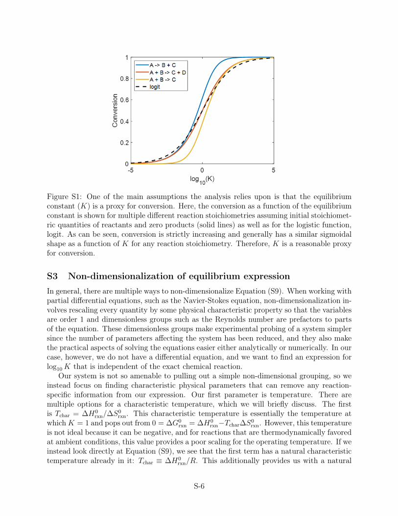
S2 Relationship between equilibrium constant K and conversion

As mentioned in the main text, we generally are looking for a value for the thermodynamicconversion, z ∈ [0, 1], when analyzing a reaction since conversion is a much more meaningfulquantity to work with when designing reactors than an equilibrium constant. Unfortunately,each reaction will have a slightly different expression for conversion as a function of theequilibrium constant, z = z(K), depending on the stoichiometry. However, there are somecommonalities in all of these conversion functions that mean that using K as a proxy forconversion is reasonable. We have shown a couple functions for conversion in terms ofthe equilibrium constant (Figure S1), where the strict increasing nature of the conversionfunction is evident. Conversion will in general always be a sigmoidal, increasing function ofK, similar to the logistic function (logit(x) = 1

1+e−x ). Moreover, z will generally span thefull range from 0 to 1 in the domain −5 < log10K < 5 regardless of stoichiometry. Becausewe are normalizing our stoichiometries (Discussion S7), our conversion functions are evenmore likely to have a similar shape and range.

In order to derive an exact expression for z as a function of K given a reaction stoichiom-etry, we will use the common RICE method (Reaction, Initialization, Change, Equilibrium).For example,

Table S3: RICE method for A + B → C + D

R A B C DI 1 1 0 0C -ε -ε ε εE 1 - ε 1 - ε ε ε

We can then write an expression for K =∏

i yi and solve for conversion, z = ε, as afunction of K algebraically or numerically.

S-5

Figure S1: One of the main assumptions the analysis relies upon is that the equilibriumconstant (K) is a proxy for conversion. Here, the conversion as a function of the equilibriumconstant is shown for multiple different reaction stoichiometries assuming initial stoichiomet-ric quantities of reactants and zero products (solid lines) as well as for the logistic function,logit. As can be seen, conversion is strictly increasing and generally has a similar sigmoidalshape as a function of K for any reaction stoichiometry. Therefore, K is a reasonable proxyfor conversion.

S3 Non-dimensionalization of equilibrium expression

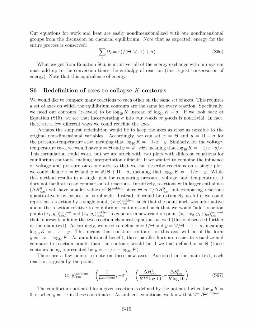
In general, there are multiple ways to non-dimensionalize Equation (S9). When working withpartial differential equations, such as the Navier-Stokes equation, non-dimensionalization in-volves rescaling every quantity by some physical characteristic property so that the variablesare order 1 and dimensionless groups such as the Reynolds number are prefactors to partsof the equation. These dimensionless groups make experimental probing of a system simplersince the number of parameters affecting the system has been reduced, and they also makethe practical aspects of solving the equations easier either analytically or numerically. In ourcase, however, we do not have a differential equation, and we want to find an expression forlog10K that is independent of the exact chemical reaction.

Our system is not so amenable to pulling out a simple non-dimensional grouping, so weinstead focus on finding characteristic physical parameters that can remove any reaction-specific information from our expression. Our first parameter is temperature. There aremultiple options for a characteristic temperature, which we will briefly discuss. The firstis Tchar = ∆H0

rxn/∆S0rxn. This characteristic temperature is essentially the temperature at

whichK = 1 and pops out from 0 = ∆G0rxn = ∆H0

rxn−Tchar∆S0rxn. However, this temperature

is not ideal because it can be negative, and for reactions that are thermodynamically favoredat ambient conditions, this value provides a poor scaling for the operating temperature. If weinstead look directly at Equation (S9), we see that the first term has a natural characteristictemperature already in it: Tchar ≡ ∆H0

rxn/R. This additionally provides us with a natural

S-6

energy scaling, ∆H0rxn. Of course, this brings up the question, why not use ∆G0

rxn as an energyscaling since it is perhaps a more relevant quantity for reaction conversion? Unfortunately,using the Gibbs free energy as our characteristic energy results in a needlessly complicatedexpression for K that makes the entire analysis less intuitive. One last detail is that wechose to define our non-dimensional temperature quantity as ∝ T instead of ∝ 1/T becausethe scaling is more intuitive with the direct proportionality.

Given a characteristic energy scaling, a characteristic voltage is simply, Echar ≡ ∆H0rxn

ne−F.

The last parameter we need to take care of is pressure. Pressure is different from therest because it already has a characteristic pressure (the reference pressure, 1 bar) built intothe equilibrium expression. However, we still want to remove any dependence on ∆nrxn. Ifwe did not want to include the logarithm in our non-dimensional quantity, we would end upwith Π =

(PP 0

)∆nrxn . This, however, is even less intuitive of a non-dimensional pressure thansimply wrapping up the entire term into a non-dimensional quantity. As a result, includinga change of base so that our expression is in base 10 instead of base e, we get the followingexpressions from the main text:

Θ ≡ RT loge 10

∆H0rxn

, (S11)

Π ≡ ∆nrxn log10

P

P 0, (S12)

Ψ ≡ ne−FE

∆H0rxn

, (S13)

σ ≡ ∆Srxn

R loge 10, (S14)

log10K = − 1

Θ− Ψ

Θ− Π + σ. (S15)

While this justification for non-dimensional groupings may appear slightly arbitrary, itnot only results in a simple equilibrium expression but also has a physical basis in the workand heat exchanges with our system, as discussed in the main text.

S4 Constant K contours and comparison of driving forces

Our non-dimensional equation is:

log10K = − 1

Θ− Ψ

Θ− Π + σ (S16)

We can see that the level curves for a given K at no applied potential (Ψ = 0) result inan inverse relationship between Π (base 10 logarithm of pressure) and Θ (temperature):

Π = (σ − log10K)− 1

Θ(S17)

Similarly, we can see that the level curves for a given K at ambient pressure (Π = 0)result in a linear relationship between Ψ (potential) and Θ (temperature):

S-7

Ψ = Θ (σ − log10K)− 1 (S18)

Last, we can see that the level curves for a givenK at ambient temperature (Θ = Θambient)result in a linear relationship between Ψ (potential) and Π (pressure):

Π = − 1

Θambient(1 + Ψ)− log10K + σ (S19)

These are the equations used to draw constant K contours in the main text (reproducedin Figure S3). Note that the constant K contours for a pressure-voltage relationship are notreaction-independent due to the appearance of Θambient, such that this cannot be plotted inuniversal form, as we are able to do in the two other cases (Figure S2). Because a voltage-pressure plot is not generalizable to all chemical reactions, we do not discuss it in detail andassume that our system relies on either voltage as a driving force (Π = 0) or pressure as adriving force (Ψ = 0), but not both simultaneously.

Figure S2: Pressure-voltage contour plot with Θambient = 0.1. Unlike the pressure-temperature and voltage-temperature plots, a pressure-voltage plot depends Θambient whichmeans it depends on ∆Hrxn (Equation S15). For this reason, it is not a universal colormapand we have included it here for completeness of visualization only. Θambient = 0.1 was chosenarbitrarily, but different values of the enthalpy of reaction will change the magnitude andsign of the contours’ slopes.

As seen visually in Figure S3, both temperature (Θ) and potential (Ψ) can easily crosscontours of constant log10K, making them powerful thermodynamic tools. Pressure, how-ever, cannot cross constant K contours as easily, requiring a large change in pressure to alterthe conversion (keep in mind that Π ∝ log10 P so an order of magnitude change in P isnecessary to change Π). Simply by looking at the colormaps of Equation S15, one can seethat qualitatively potential is a better choice than pressure for improving conversion.

We can better compare these thermodynamic driving forces quantitatively by comparingthe derivatives of log10K with respect to each variable. Taking the partial derivatives ofEquation S15, we get:

S-8

Figure S3: Plots of Equation S15, reproduced from main text. Every reaction can be mappedonto these plots. When no voltage is applied (Ψ = 0), the contours of how pressure andtemperature affect the equilibrium are visualized (left). At ambient pressure (Π = 0),the contours of how voltage and temperature affect the equilibrium are visualized (right).Qualitatively, crossing the constant K contours using pressure is more difficult than usingvoltage or temperature. Note that the colorbar axis is log10K − σ so that the plot remainsindependent of reaction; different reactions will essentially provide a constant shift from σthat does not change the shape of the plot. Note that crossing Θ = 0 for a given reactionis impossible since the sign of Θ is determined by the reaction enthalpy (a fixed quantityassuming ∆CP,rxn = 0).

(∂ log10K

∂Π

)Θ,Ψ

= −1 (S20)(∂ log10K

∂Θ

)Π,Ψ

=1

Θ2(1 + Ψ) (S21)(

∂ log10K

∂Ψ

)Θ,Π

= − 1

Θ(S22)

We can see right away from these derivatives that, given Θ < 1 (generally true forreasonable reaction enthalpies and operating temperatures, Table S4), log10K will scalemore favorably with voltage (Ψ) and temperature (Θ) than with pressure (Π). Additionally,given that Π ∝ logP , K has a logarithmic relationship with pressure, making it a relativelypoorer driving force compared to temperature and voltage. In order to better comparethese derivatives, we can compare the derivatives of log10K with respect to log10 Θ andlog10 Ψ. This would put them on equal footing with the derivative with respect to Π sothat all the derivatives are with respect to the logarithm of a dimensional thermodynamicparameter. Additionally, this removes some of the arbitrariness of the non-dimensionalizationsince instead of comparing a "unit" increase in Θ to a "unit" increase in Ψ and Π, we arenow comparing relative increases in dimensional thermodynamic parameters (e.g., we arecomparing the effect of doubling temperature, pressure, and voltage).

S-9

(∂ log10K

∂Π

)Θ,Ψ

= −1 (S23)(∂ log10K

∂ log10 Θ

)Π,Ψ

=loge 10

Θ(1 + Ψ) (S24)(

∂ log10K

∂ log10 Ψ

)Θ,Π

= −Ψ

Θloge 10 (S25)

These derivatives further support that qualitatively, crossing voltage and temperaturecontours is easier and more effective than crossing pressure contours since they have relativelylarger derivatives than the derivative with respect to Π. We additionally see that at lowvalues of Ψ, crossing voltage contours may be less effective, but that with moderate to largevalues of Ψ (Ψ can easily increase above 2 in some reactions with smaller |∆H0

rxn|, TableS4), crossing voltage contours becomes significantly more effective than crossing pressurecontours. Crossing temperature contours remains perhaps the most effective at increasingK, but temperature is limited in that we cannot practically go to operating temperaturesabove ca. 1500 K, which is insufficient to drive some reactions.

We have so far stated as fact that Θ < 1 for many reactions, and to back this up, I haveprovided values for Θambient for ammonia synthesis and water splitting:

1

2N2 +

3

2H2 −−→ NH3 , (R1)

H2O −−→ H2 +1

2O2 . (R2)

Table S4: Reaction parameters for ammonia synthesis and water splitting

Rxn ∆H0rxn (kJ/mol) ∆S0

rxn (J/mol.K)∑

i=gas νi n Θambient E at Ψ = 1

Eq. R1 -46 -99 -1 3 -0.12 -0.16 VEq. R2 242 44 0.5 2 0.024 1.25 V

We can see that for these very different reactions, Θambient and Ψ have values as we havedescribed above.

S5 Derivation of work and energy exchange

We want to convert our chemical reaction system away from the variables T , P , and E, whichare not directly comparable, to quantities that are directly comparable. In particular, wewant to compare relevant work and energy quantities for our system, specifically mechanicalwork input (WM,on), heat input (Qon) and electrochemical work input (WE,on). All of theseparameters have units of Watts, and we will assume continuous, steady state operationof our system with each step being reversible. Additionally, we will continue toassume that all of our mixtures are ideal mixtures of ideal gases. As we all know fromthermodynamics, work and heat flow are path variables and should depend on exactly how

S-10

we operate our system. However, if we constrain our system to operate with one heat bath(e.g., the atmosphere), then all reversible paths will result in the same work and heat flux.We have introduced one additional parameter to our system, T bath, but in return work andheat flux become state functions.

The system we will work with is shown in Figure S4, a variation on a Van’t Hoff Equi-librium box[2, 3]. In particular, we will first change our system from ambient conditions toreaction conditions, operate the reaction for some extent of reaction at constant T, P, andE, and then return our system to ambient conditions.

Figure S4: Model for calculating work and heat flow for our system. Each box is a separateunit we will analyze as described in the text. Note that as written, nin and nout are vectorsof mole flowrates with nout = nin − ξν (ξ is the extent of reaction between 0 and 1 and ν isa vector of the stoichiometric coefficients)

We will treat each sub-unit of Figure S4 in turn. First, let’s look at the unit that changesthe T and P to operating conditions. We can do an entropy (Second law) balance over thisunit and get the following equation for the heat flow.

Suniverse = Sunit + Senvironment − ninS(T0, P0, E0) + ninS(T, P,E) (S26)

0 = − Qon

T bath+ nin

(CP,rxts log

T

T0

−R logP

P0

)(S27)

Qon = ninTbath

(CP,rxts log

T

T0

−R logP

P0

)(S28)

We have assumed steady state (Sunit = 0) and reversible (Suniverse = 0), and have usedthe entropy for an ideal gas. Additionally, R is the ideal gas constant and CP,rxts is the molaraverage CP of the reactant mixture. We can next perform an energy (First Law) balance toget the mechanical work on the system.

U = Qon + WM,on + ninH(T0, P0, E0)− ninH(T, P,E) (S29)

0 = Qon + WM,on + ninCP,rxts(T0 − T ) (S30)

WM,on = ninCP,rxts(T − T0)− ninTbath

(CP,rxts log

T

T0

−R logP

P0

)(S31)

Again, we have assumed steady state and an ideal gas with the enthalpy being only afunction of temperature. A few important items to note about these equations: First, we needto specify T bath. We chose this additional parameter instead of a specific thermodynamic

S-11

path to increase generality of our analysis. In practice, though, our derivation is not sodifferent from an adiabatic compressor followed by a heat exchanger. Second, because ourpath is reversible, the work and heat flow on the unit after the reactor will essentially be thesame expression except with nout instead of nin and CP,prds instead of CP,rxts. Third, becauseour system is reversible, the work we calculate is the maximum possible work by our system(or the minium work on our system).

The remaining unit we need to analyze is the reaction unit itself (the post-reactor unit isidentical to the pre-reactor unit with some sign changes). We will follow the same procedureas above. Since our reaction is at constant T and P, the environment must also be at T andP for the sake of thermodynamic consistency in our derivation. First, a second law balancegives:

Qon = ξT

(∆S0

rxn + ∆CP,rxn logT

T 0−∆nrxnR log

P

P 0

)(S32)

= ξT∆Srxn (S33)

A first law energy balance gives:

WM,on + WE,on = −ξT(

∆S0rxn + ∆CP,rxn log

T

T 0−∆nrxnR log

P

P 0

)+ ξ

(∆H0

rxn + ∆CP,rxn(T − T 0))

(S34)

= ξ∆Grxn(T, P ) (S35)

This makes intuitive sense, but does not allow for the case where the reaction doesnot allow for mechanical work and the reaction’s mechanical work is dissipated as heat.Incorporating the known electrical work allows us to write the following expressions:

WE,on = −ξnFE (S36)

WM,on ≤ ξ(∆Grxn(T, P ) + nFE) (S37)

Qon = ξ(∆H0

rxn + ∆CP,rxn(T − T 0))−(WM,on + WE,on

)(S38)

Combining Equations S36, S37, and S38 along with Equations S28 and S31 for the preand post change in state give us an expression for the total work and heat flow of the entiresystem.

WE,on = ηrxn,WEW rxnE,on (S39)

WM,on = ηpre,W W preM,on + ηrxn,WMW rxn

M,on + ηpost,W W postM,on (S40)

Qon = ηpre,QQpreon + ηrxn,QQrxn

on + ηpost,QQposton (S41)

Here all of the ηi represent efficiencies that can be put in if more information is know abouta system (e.g., if you will not be using an expander to retrieve work ηpost,W = 0). Forthe sake of analysis, we will assume that all ηi = 1, representing the theoretical minimum

S-12

work performed on our system and its corresponding heat flow. We then get the followingexpression for the total work and heat flow in our system given a certain T and P (rememberthat the extent of reaction is also just a function of T and P). In this derivation we assumethat mechanical work can be exchanged with the reactor.

WM,on = (ninCP,rxts − noutCP,prds)(T − T0) (S42)

− T bath

((ninCP,rxts − noutCP,prds) log

T

T0

− (nin − nout)R logP

P0

)(S43)

+ ξ(∆Grxn(T, P ) + nFE) (S44)

= −ξ∆CP,rxn(T − T0) + ξT bath

(∆CP,rxn log

T

T0

−∆nrxnR logP

P0

)(S45)

+ ξ(∆Grxn(T, P ) + nFE) (S46)

WM,on = ξ

(∆G0

rxn + (T bath − T )

[∆CP,rxn log

T

T0

−∆nrxnR logP

P0

]+ nFE

)(S47)

Qon = T bath

((ninCP,rxts − noutCP,prds) log

T

T0

− (nin − nout)R logP

P0

)(S48)

+ ξ(∆H0

rxn + ∆CP,rxn(T − T 0)−∆Grxn(T, P ))

(S49)

= −ξT bath

(∆CP,rxn log

T

T0

−∆nrxnR logP

P0

)(S50)

+ ξ(∆H0

rxn + ∆CP,rxn(T − T 0)−∆Grxn(T, P ))

(S51)

Qon = ξ

(T∆S0

rxn − (T bath − T )

[∆CP,rxn log

T

T0

−∆nrxnR logP

P0

])(S52)

WE,on = −ξnFE (S53)

If we assume that no mechanical work can be exchanged with the reactor (areasonable industrial situation that corresponds to us relaxing the constraint Suniverse = 0for the reactor unit itself), we get the following:

WE,on = −ξnFE (S54)

WM,on = ξ

(−∆CP,rxn(T − T0) + T bath

[∆CP,rxn log

T

T0

−∆nrxnR logP

P0

])(S55)

Qon = ξ

(−T bath

[∆CP,rxn log

T

T0

−∆nrxnR logP

P0

]+ ∆H0

rxn + ∆CP,rxn(T − T0) + nFE

)(S56)

Interestingly enough, even though we began this analysis allowing enthalpy to vary withtemperature, we find that in these final expressions for work and heat flow that the enthalpicterms all contain ∆CP,rxn. We previously assumed this value to be zero, and while this is not a

S-13

good assumption for quantitative results, it is a reasonable assumption to qualitativelystudy the system. From here forward, we will assume that no mechanical work isexchanged between the reactor and the environment. With these assumptions, weget the following expressions for work and heat flows:

WE,on = −ξnFE (S57)

WM,on = −ξ∆nrxnRTbath log

P

P0

(S58)

Qon = ξ

(∆nrxnRT

bath logP

P0

+ ∆H0rxn + nFE

)(S59)

These are remarkably simple expressions that still make qualitative sense. The electricalwork depends on the voltage and conversion by definition. The mechanical work dependson the conversion and the pressure, with any temperature terms having been neglectedat this point in the simplification. The heat flow is a function of the reaction enthalpy,the pressure, and the potential as well as conversion. We note that temperature does notappear explicitly in these expressions due to the fact that the temperature components cancelout to enough of a degree that we neglect them with our assumption that the enthalpy ofreaction is independent of temperature. However, these expressions still depend strongly ontemperature since the conversion will depend strongly on temperature.

A major assumption that we are making is that the heat bath used to bring the reactantsto operating conditions and the heat bath used to bring the products to ambient conditions isat the same T bath. This is likely a poor assumption in practice, but for the sake of qualitativeanalysis it is sufficient to give us an idea of the functional form of the work and heat fluxterms in terms of simple parameters while avoiding complications from the various heatcapacities of reactants and products.

As it turns out, we can write our equations for work and heat flow in non-dimensionalform as in the main text. Let us define new non-dimensional quantities:

ΩW,E =WE,on

∆H0rxn

(S60)

ΩW,M =WM,on

∆H0rxn

(S61)

ΩQ =Won

∆H0rxn

(S62)

Additionally, note that ξ = z(log10Keq) = z(f(Θ,Ψ,Π)+σ), where f = −1/Θ−Ψ/Θ−Π.The exact function form of ξ depends on the reaction, but we know it is roughly logistic inshape and spans 0 to 1 from log10Keq = −5 to log10Keq = 5, respectively.

We can now write:

ΩW,E = −z(f(Θ,Ψ,Π) + σ)Ψ (S63)ΩW,M = −z(f(Θ,Ψ,Π) + σ)ΘbathΠ (S64)ΩQ = z(f(Θ,Ψ,Π) + σ)(ΘbathΠ + Ψ + 1) (S65)

S-14

Our equations for work and heat are easily nondimensionalized with our nondimensionalgroups from the discussion on chemical equilibrium. Note that as expected, energy for theentire process is conserved: ∑

i

Ωi = z(f(Θ,Ψ,Π) + σ) (S66)

What we get from Equation S66, is intuitive: all of the energy exchange with our systemmust add up to the conversion times the enthalpy of reaction (this is just conservation ofenergy). Note that this equivalence of energy

S6 Redefinition of axes to collapse K contours

We would like to compare many reactions to each other on the same set of axes. This requiresa set of axes on which the equilibrium contours are the same for every reaction. Specifically,we need our contours (z-levels) to be log10K instead of log10K − σ. If we look back atEquation (S15), we see that incorporating σ into our x-axis or y-axis is nontrivial. In fact,there are a few different ways we could redefine the axes.

Perhaps the simplest redefinition would be to keep the axes as close as possible to theoriginal non-dimensional variables. Accordingly, we can set x = Θ and y = Π − σ forthe pressure-temperature case, meaning that log10K = −1/x− y. Similarly, for the voltage-temperature case, we would have x = Θ and y = Ψ−σΘ, meaning that log10K = −1/x−y/x.This formulation could work, but we are stuck with two plots with different equations forequilibrium contours, making interpretation difficult. If we wanted to combine the influenceof voltage and pressure onto one axis so that we can describe reactions on a single plot,we could define x = Θ and y = Ψ/Θ + Π − σ, meaning that log10K = −1/x − y. Whilethis method results in a single plot for comparing pressure, voltage, and temperature, itdoes not facilitate easy comparison of reactions. Intuitively, reactions with larger enthalpies(∆H0

rxn) will have smaller values of Θambient since Θ ∝ 1/∆H0rxn, but comparing reactions

quantitatively by inspection is difficult. Instead, it would be extremely useful if we couldrepresent a reaction by a single point, (x, y)ambient

rxn , such that the point itself was informativeabout the reaction relative to equilibrium contours and such that we would “add” reactionpoints (x1, y1)ambient

rxn,1 and (x2, y2)ambientrxn,2 to generate a new reaction point (x1+x2, y1+y2)ambient

rxn

that represents adding the two reaction chemical equations as well (this is discussed furtherin the main text). Accordingly, we need to define x = 1/Θ and y = Ψ/Θ + Π− σ, meaninglog10K = −x − y. This means that constant contours on this axis will be of the formy = −x − log10K. As an additional benefit, these parallel lines are easier to visualize andcompare to reaction points than the contours would be if we had defined x = Θ (thosecontours being represented by y = −1/x− log10K).

There are a few points to note on these new axes. As noted in the main text, eachreaction is given by the point:

(x, y)ambientrxn =

(1

Θambient,−σ

)=

(∆H0

rxn

RT 0 log 10,− ∆S0

rxn

R log 10

)(S67)

The equilibrium potential for a given reaction is defined by the potential when log10K =0, or when y = −x in these coordinates. At ambient conditions, we know that Ψeq/Θambient−

S-15

σ = yeq = −xambient. From this, we can get:

Ψeq = Θambient(yeq + σ) (S68)= Θambient(yeq − yambient) (S69)= (yeq − yambient)/xambient (S70)= −(yeq − yambient)/yeq (S71)

= −1 +yambient

yeq(S72)

Ψeq = −1− yambient

xambient(S73)

We can see that the non-dimensional equilibrium potential is proportional to the ratioof yambient to yeq, or equivalently the ratio yambient to xambient which is the slope of a linefrom (0, 0) to (x, y)ambient

rxn , a simple and intuitive read from the plot. However, there is aneven simpler measure of equilibrium potential available from this plot that makes these axesextremely powerful and is described in detail in Discussion S7.

In these redefined axes, a change in voltage or pressure will result in a vertical movementon the axes, and an increase (decrease) in temperature corresponds to a movement toward(away from) the point (0,Π − σ) (movement along the line given by y = −σ + Π + Ψx).A reproduction of the comparison of multiple reactions from the text if provided with theaddition of vertical lines representing an increase in pressure by an order of magnitude(Figure S5).

S7 Scaling of reaction stoichiometry to compare reactions

In order to make a proper comparison between reactions, we need to normalize the stoi-chiometry. To do this, each reaction is scaled to a fixed number of electrons transferred inthe reaction (fixed ne−). This means that each of ∆Hrxn, ∆Srxn, and ∆nrxn are rescaled suchthat ne− = ρ. The big question is: what value of ρ should be used? A value between 1 and4 makes the most sense as it leads to reactions collapsing visually on these axes such thatthe reactions can be compared easily while still being spaced sufficiently apart. To aid withreadability, it makes sense to scale to a number that will result in a meaningful point (x, y).We have therefore chosen to scale to ne− = 2.956. This value, although it appears arbitrary,is actually chosen such that a reaction at point (x, y) will have a dimensional equilibriumpotential Eeq = −20(x+ y) (Eeq in mV).

We can see that for a reaction defined by,

(x, y)ambientrxn =

(1

ΘRT,−σ

)=

(∆H0

rxn

RT 0 log 10,− ∆S0

rxn

R log 10

)(S74)

the sum of the coordinates is

S-16

Figure S5: Reproduction from main text of comparison of multiple reactions on the sameaxes. Each point represents a chemical reaction, with color denoting whether the reaction istypically conducted thermochemically (pink) or electrochemically (blue). Each reaction pointis such that (x, y)ambient ∝ (∆H0

rxn,−∆S0rxn) and can be interpreted as described in Figure S6.

Vertical lines represent an increase in pressure by one order of magnitude. The green shadingindicates the area where an elevated temperature of less than ∼ 1500 K can reachK = 1, anda quantitative visual divide based on reaction enthalpies and entropies distinguishes betweenreactions driven with electrochemistry versus those driven with thermochemistry. Note thatthe stoichiometry depicted in the legend is for readability; all reactions have been scaled tohave the same number of electrons for best comparison (Supplemental Derivation S7). To beconsistent, chemical formulas were used for all species in the legend, but the following formu-las are not unique and refer to the specified chemical: C3H6O (propanal), C2H4O (ethyleneoxide), C3H6 (propene), C6H6 (benzene), C3H3N (acrylonitrile), and C6H8N2 (adiponitrile).Raw thermodynamic data given in Tables S1 and S2. [4, 1, 6, 5].

(x+ y) =∆H0

rxn

RT 0 log 10− ∆S0

rxn

R log 10(S75)

=∆G0

rxn

RT 0 log 10(S76)

=−ne−F

RT 0 log 10Eeq (S77)

Solving for ne− such that −nFRT 0 log 10

= −0.05 mV−1 (arbitrarily chosen so that the pointswill be well spaced on the plot and the numbers will be easy for mental math) gives ne− =2.956. Unlike previously where we equated the non-dimensional equilibrium potential with aratio of yambient to xambient, here we see that the dimensional equilibrium potential can be readdirectly from this plot. As a corollary to this fact, we can see that reaction points that have|Eeq| ≤ 1 V must satisfy the condition that 1000 mV ≥ | − 20(x+ y)|, or equivalently mustsatisfy −50− x ≤ y ≤ 50− x. Although we have not drawn these lines, they unsurprisinglyshow that voltages of order 1 V are sufficient to drive thermodynamic conversion of mostchemical reactions encountered in the wild.

S-17

Figure S6: Reproduction from main text. Redefined axes such that all reactions have thesame equilibriumK contours. A contour corresponding toK = 1 is indicated with a diagonalblack line. The filled red diamonds represent an example reaction point at ambient conditionsgiven by Equation (S67). An increase in either pressure (Π) or voltage (Ψ) is a verticalmovement on these axes (A, new reaction point given by blue square) and an increase intemperature (Θ) is a movement towards the point (0,Π − σ) (A, new reaction point givenby blue circle, movement along the line connecting to the empty blue diamond). As shown,the distance from the reaction point to the y-axis is proportional to ∆H0

rxn, the distanceto the x-axis is proportional to ∆S0

rxn, and the distance to the solid black line (y = −x) isproportional to the dimensional equilibrium potential of the reaction (B). Further details inSupplemental Derivations S5 and S6

S8 Simple Descriptors

Some of the major points about reaction feasibility and thermodynamic equilibrium can bedetermined from simple descriptors without the need for our non-dimensionalization scheme.For example, simply looking at the sign of ∆Grxn at a given temperature will tell us whetherthe reaction is thermodynamically favorable, and Tchar = ∆H0

rxn/∆S0rxn provides us with

a metric of whether temperature alone can drive a given reaction to thermodynamic equi-librium. Other potential descriptors such as

∑i νi for a reaction tell us the influence of

pressure and Eeq = ∆Grxn/nF gives an idea of how much voltage is necessary to drive thereaction. Individually, each of these descriptors is extremely useful, but they unfortunatelymust be calculated for each specific reaction, often at various operating conditions. Thesedescriptors are therefore useful, but do not contain the same amount of information as ourvisualization in Figure S5. As an example, using ∆Grxn and Tchar as descriptors, we haveplotted the same data as in Figure S5 on new axes (Figure S7). While discrimination viathese quantities can tell us whether a reaction is capable of being driven by temperature toequilibrium conversion, they do not provide information about the magnitude of the influ-ence of temperature, pressure, and voltage, and they do not provide any information on theinfluence of pressure on the reaction. When temperature, pressure, and voltage deviate fromambient conditions, the new equilibrium conversion is readily apparent on Figure S5 as theaxes scale with these thermodynamic quantities as discussed in the main text. Additionally,the influence of pressure on a reaction can be quickly ascertained on our axes based on the

S-18

y-value of the point (or explicitly shown in Figure S5 with the vertical lines), whereas the roleof pressure is difficult to determine from the Gibbs free energy of reaction or the equilibriumtemperature. Because our axes allow for quantification of the influence of thermodynamicparameters on the equilibrium conversion, our axes can be used to investigate such questionsas: what is the equilibrium conversion of ammonia synthesis at operating conditions? And:which reactions can rely on pressure to increase equilibrium conversion at conditions whichfacilitate fast kinetics? The answers to these questions are not novel—we could easily gatheradditional descriptors similar to those mentioned above that would encompass more aspectsof the system. However, with our carefully chosen non-dimensional scheme, we can visualizeall of these descriptors on a single plot for multiple reactions instead of requiring a list ofdescriptors for each individual reaction at every temperature, pressure, and voltage of inter-est. We can also add and subtract reactions on our proposed axes for simple exploration ofpossible reactants and products as discussed in the main text.

Figure S7: Transformation of Figure S5 data to potential binary descriptors as axes. Al-though some of the information is preserved on these axes, there is a significant loss ofinformation as described in SI Appendix, Discussion 8.

S-19

Supplemental References

References[1] Dortmund Data Bank, 2020.

[2] N. M. Bazhin. Mechanism of electric energy production in galvanic and concentrationcells. Journal of Engineering Thermophysics, 20(3):302–307, 2011.

[3] N. M. Bazhin and V. N. Parmon. Conversion of the chemical reaction energy into usefulwork in the Van’t Hoff equilibrium box. Journal of Chemical Education, 84(6):1053–1055,2007.

[4] D.R. Burgess. Thermochemical Data. In P.J. Linstrom and W.G. Mallard, editors,NIST Chemistry WebBook, NIST Standard Reference Database Number 69, chapter Ther-mochem. National Institute of Standards and Technology, Gaithersburg, MD.

[5] Connie W. Gao, Joshua W. Allen, William H. Green, and Richard H. West. ReactionMechanism Generator: Automatic construction of chemical kinetic mechanisms. Com-puter Physics Communications, 203:212–225, 2016.

[6] Norbert Adolph Lange. Lange’s Handbook of Chemistry. McGraw-Hill, Inc., 15 edition,1999.

S-20

download fileview on ChemRxivSI.pdf (1.36 MiB)