THERMODYNAMIC EQUILIBRIUM COMPUTATION OF SYSTEMS WITH AN ARBITRARY NUMBER OF PHASES FLOW MODELING WITH LATTICE BOLTZMANN METHODS: APPLICATION FOR RESERVOIR SIMULATION A REPORT SUBMITTED TO THE DEPARTMENT OF ENERGY RESOURCES ENGINEERING OF STANFORD UNIVERSITY IN PARTIAL FULFILLMENT OF THE REQUIREMENTS FOR THE DEGREE OF MASTER OF SCIENCE By C´ edric Frac` es Gasmi August 2010
Transcript
THERMODYNAMIC EQUILIBRIUM
COMPUTATION OF SYSTEMS WITH AN
ARBITRARY NUMBER OF PHASES
FLOW MODELING WITH LATTICE
BOLTZMANN METHODS: APPLICATION FOR
RESERVOIR SIMULATION
A REPORT
SUBMITTED TO THE DEPARTMENT OF ENERGY RESOURCES
ENGINEERING
OF STANFORD UNIVERSITY
IN PARTIAL FULFILLMENT OF THE REQUIREMENTS
FOR THE DEGREE OF
MASTER OF SCIENCE
By
Cedric Fraces Gasmi
August 2010
I certify that I have read this report and that in my
opinion it is fully adequate, in scope and in quality, as
partial fulfillment of the degree of Master of Science in
Energy Resources Engineering.
Hamdi Tchelepi(Principal advisor)
ii
Abstract
Reservoir recovery processes involve complex mass and heat transfer between the
injected fluid and the resident rock-fluid system. Thermal-compositional reservoir
simulators can be used to plan such displacement processes, in which the phase behav-
ior is computed with an Equation of State (EoS). These thermodynamic-equilibrium
computations include phase-stability tests and flash calculations, and can consume a
significant fraction of the total simulation time, especially for highly detailed reservoir
models and a large number of components. Here, we propose a general Compositional
Space Parameterization (CSP) method for complex mixtures, especially those where
more than two fluid phases can coexist in parts of the parameter space. For a given
pressure (P), temperature (T) and overall composition, a unique tie-simplex (tie-line
for two phases, tie-triangle for three phases, etc.) can be defined. For a particular
composition at P and T, the tie-simplex provides the necessary phase equilibrium
information (i.e., phase state and phase compositions). For compositional flow simu-
lation, a set of tie-simplexes can be calculated in a preprocessing step, or adaptively
constructed during the simulation. The tie-simplex representation can be used to
replace standard phase-equilibrium calculations completely, or it can be used as an
initial guess for standard EoS calculations. Challenging examples with two and three
phases are presented to validate this tie-simplex CSP approach. Standard EoS meth-
ods, which are widely used in industrial compositional simulators, are compared with
CSP-based simulations for problems with large numbers of components and complex
two- and three-phase behaviors spanning wide ranges of pressure and temperature.
The numerical experiments indicate that our multi-dimensional tie-simplex represen-
tation combined with linear pressure and temperature interpolation in tie-simplex
iii
space, which is implemented as an adaptive tabulation strategy, leads to highly ro-
bust and efficient computations of the phase behavior associated with compositional
flow simulation.
The characterization of reservoir models requires information such as porosity,
permeability, relative permeability, and capillary pressure. Various techniques are
used to describe the pore-scale details and model the flow dynamics. This knowl-
edge is then used to estimate the macroscopic (Darcy-scale) properties and solve the
macroscopic equations governing flow and transport in very large domains. We sur-
vey different pore-scale simulators based on Lattice Boltzman methods. We present
qualitative and quantitative results obtained from available simulators, as well as,
our own implementation of existing algorithms. We document and test different ap-
proaches and give an overview of the advantages and the challenges that remain to
be resolved.
iv
Acknowledgments
I would like to express my sincere gratitude to my adviser Prof. Hamdi Tchelepi for
his time, confidence, support and guidance. None of this would have been possible
without him. I also wish to thank Dr. Denis Voskov for his trust, valuable comments
and help.
I wish to thank Lisette Quettier and Arthur Moncorge (Total) who gave me the
opportunity to come to Stanford and initiated this adventure. I would also like
to thank the Stanford University Petroleum Research Institute (SUPRI-B), and its
affiliates for their financial support.
I am very grateful to the staff of the Department of Petroleum Engineering who
has contributed in creating an ideal environment for the development of research
projects.
I thank Youngseuk Kheem, Ratnanabha Sain and Tapan Mukerji for use of their
Lattice Boltzmann Simulation code.
I would like to thank warmheartedly my classmates, friends and beloved office-
mates, whose help and friendship made my stay at Stanford a wonderful experience.
Special thanks to Guillaume Moog, Antoine Bertoncello, Mathieu Rousset, Sebastien
Matringe, Bruno Dujardin, Danny Rojas, Mehrdad Honarkhah, Markus Buchgraber,
Mohammad Al Dossary, Ekin Ozdogan, Israel Reyna, Mohammad Shahvali, Obi Ise-
bor, Alejandro Leiva.
Finally, I thank my family for their constant support and belief in me.
v
Contents
Abstract iii
Acknowledgments v
Table of Contents vi
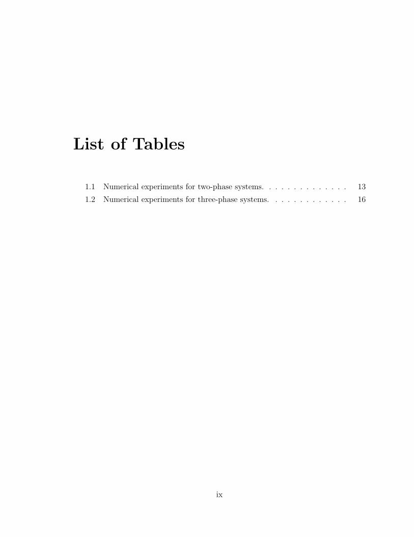
List of Tables ix
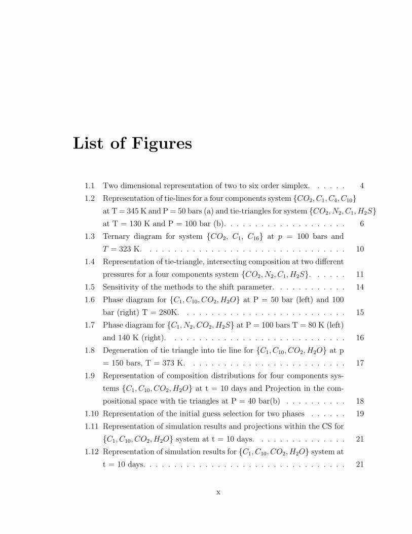
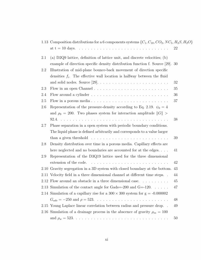
List of Figures x
1 Thermodynamic Equilibrium: Arbitrary Number of Phases 1
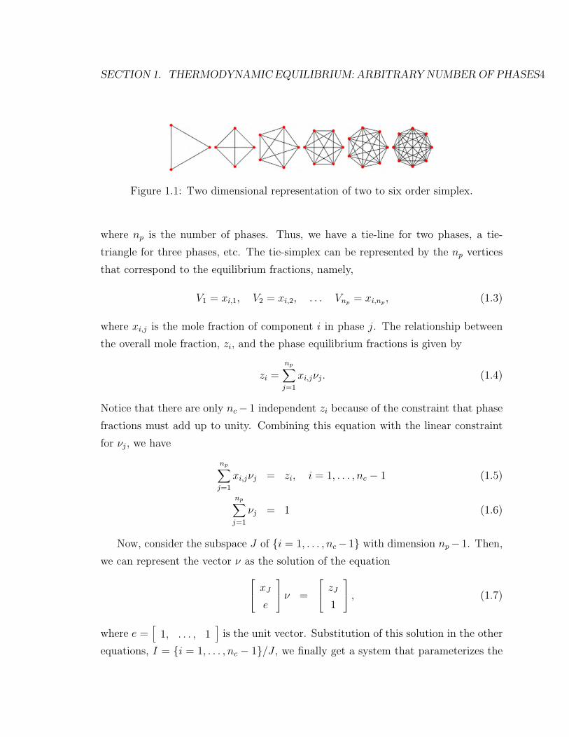
1.1 Two dimensional representation of two to six order simplex. . . . . . 4
1.2 Representation of tie-lines for a four components system CO2, C1, C4, C10at T = 345 K and P = 50 bars (a) and tie-triangles for system CO2, N2, C1, H2Sat T = 130 K and P = 100 bar (b). . . . . . . . . . . . . . . . . . . . 6
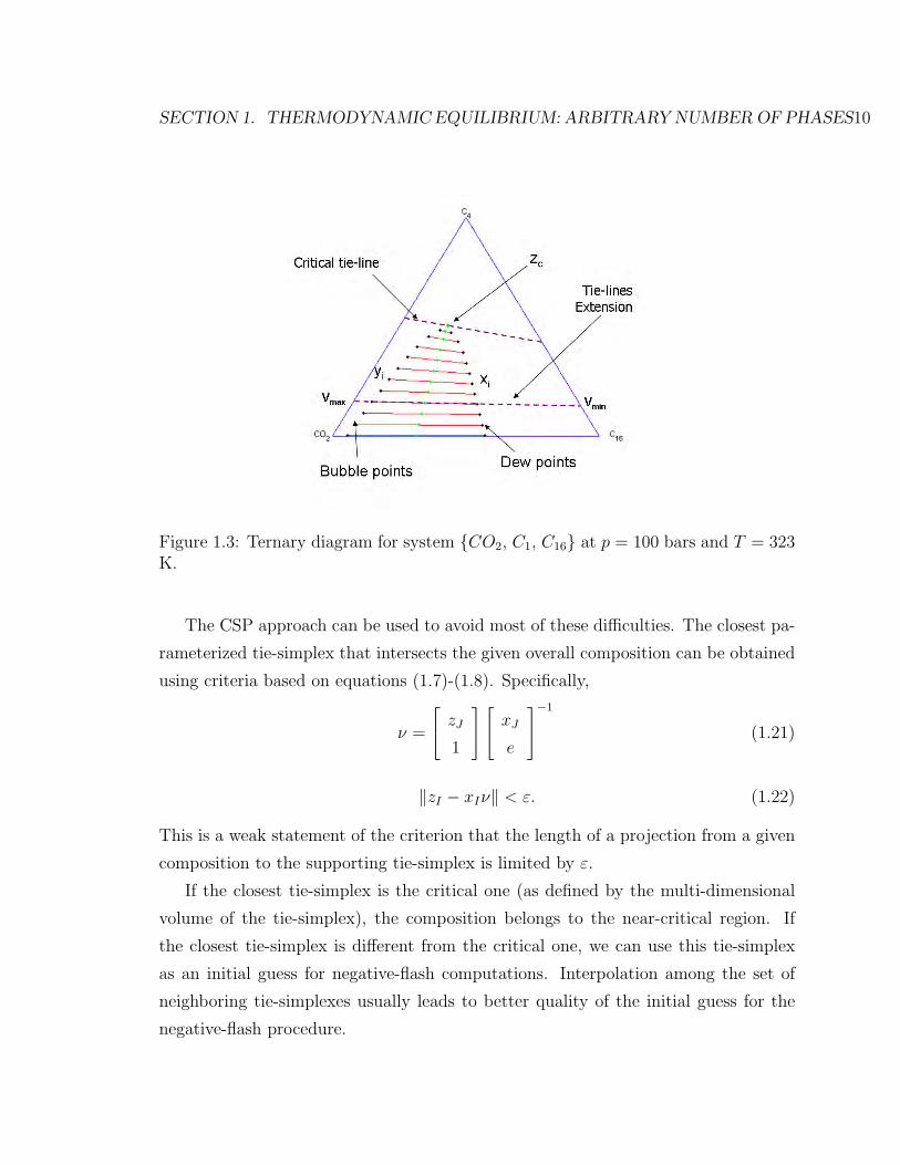
1.3 Ternary diagram for system CO2, C1, C16 at p = 100 bars and
Enhanced oil recovery (EOR) of heavy hydrocarbons usually involve thermal pro-
cesses that are described using a thermal-compositional model [3]. The equations
that describe the flow, transport and thermodynamic behavior include mass and en-
ergy conservation and thermodynamic-equilibrium relations. The accurate descrip-
tion of the phase behavior of the multi-component multiphase mixtures as a function
of pressure and temperature is a major challenge in compositional flow simulation. A
thermodynamic approach using an Equations of State (EoS) is usually employed to
describe the phase behavior. It is possible to determine the state of a mixture (phases)
based only on the overall component compositions, pressure, and temperature. The
use of an EoS based approach makes the simulation process time consuming. The
thermodynamic-equilibrium equations are usually solved iteratively for each computa-
tional gridblock at every Newton iteration during a time step. Accurate and efficient
integration of thermodynamic computations in compositional simulation has been the
subject of several recent books [1], [8].
One of the widely used simplifications is the assumption of constant K-values, [4].
In this approach, the component equilibrium ratios between are taken to be a function
1
SECTION 1. THERMODYNAMIC EQUILIBRIUM: ARBITRARY NUMBER OF PHASES2
of pressure and temperature only, and this reduces the complexity of dealing with
the nonlinear behaviors due to compositional dependence of the phase equilibrium
equations. Extensions for this K-value approach have been proposed, [11], in which
the equilibrium ratios are assumed to depend on the overall fraction of one of the
components. However, this approximation is accurate only for low temperatures and
can lead to difficulties in representing the phase behavior in the near-critical region.
The determination of the phase state of the mixture is necessary to solve the sys-
tem of conservation laws that describes multi-component, multi-phase transport in
porous media. Once the phase state of a given gridblock is determined for the current
nonlinear (Newton) iteration, the solution for the next iteration can be computed.
The phase-state definition is an important aspect of compositional simulation. One
needs to track the appearance and disappearance of the various phases. The disap-
pearance of a phase is detected based on the saturation. When a phase saturation
becomes negative, the phase is assumed to have disappeared. Phase appearance is
usually treated using a phase stability analysis [9]. In this case, we need to determine
the equilibrium state by computing the tangent plane distance (TPD) of the Gibbs
energy function. This procedure must be performed for every single-phase cell at
every nonlinear iteration of the flow computation process. It can be time consuming,
especially when the numbers of phases and components are large.
Michelsen et al. [6] presented a method to speed up the phase behavior computa-
tions for compositional mixtures in pipe flow. They proposed criteria for avoiding the
phase stability test in single-phase fluids. This approach is very efficient for transient
simulation where the compositions change slowly. Since most nonlinear solvers for
reservoir simulation include limits on the compositional changes during an iteration,
this method can be applied to gas injection processes as well. However, it is difficult
to extend this method to systems with more than two phases, or for more sophisti-
cated nonlinear solvers, in which significant changes in the mixture composition in
gridblock can take place.
While two-phase EoS computations associated with compositional flow simula-
tion are becoming quite robust and efficient, reliable methods for handling multi-
component fluids with more than two phases are generally lacking. The purpose of
SECTION 1. THERMODYNAMIC EQUILIBRIUM: ARBITRARY NUMBER OF PHASES3
this work is to provide an alternative method for phase-behavior computations in
flow simulation for systems with an arbitrary number of phases. Specifically, we pro-
pose a negative-flash based strategy within a compositional space parametrization
(CSP) framework. Comparisons with standard EoS based approaches are used to
demonstrate the effectiveness of our method.
1.2 Compositional space parametrization for sys-
tems with arbitrary numbers of phases
We summarize the compositional space parameterization (CSP) framework, which
serves as the basis of our approach. The details of the CSP framework are presented
in [16].
1.2.1 General Thermodynamic Parameterization
The overall mole fraction of a component, zi, is usually used in thermodynamic equi-
librium calculations. The independent mole fractions form a subset of <nc , where nc
is the number of components, and can be expressed as follows:
∆nc−1 = (z1 . . . znc) ∈ <nc |∑
zi = 1, zi ≥ 0, ∀i. (1.1)
This relation defines an (nc − 1)-dimensional simplex in <nc . Geometrically, this
means we can represent the compositional space using a line for two components, a
triangle for three component (∆2), a tetrahedron for four components (∆3), and so
on. Fig. 1.2.1 shows the projection in two dimension of a few simplexes. For higher
dimensions, the visualization is more complex.
In a multi-component multi-phase system, the state of thermodynamic equilibrium
is defined by the volume fractions of the phases, νj, and can be represented using an
(np − 1)-dimensional tie-simplex defined as
∆np−1 = (ν1 . . . νnp) ∈ <np |∑
νj = 1, νj ≥ 0 ∀j. (1.2)
SECTION 1. THERMODYNAMIC EQUILIBRIUM: ARBITRARY NUMBER OF PHASES4
Figure 1.1: Two dimensional representation of two to six order simplex.
where np is the number of phases. Thus, we have a tie-line for two phases, a tie-
triangle for three phases, etc. The tie-simplex can be represented by the np vertices
that correspond to the equilibrium fractions, namely,
V1 = xi,1, V2 = xi,2, . . . Vnp = xi,np , (1.3)
where xi,j is the mole fraction of component i in phase j. The relationship between
the overall mole fraction, zi, and the phase equilibrium fractions is given by
zi =np∑j=1
xi,jνj. (1.4)
Notice that there are only nc− 1 independent zi because of the constraint that phase
fractions must add up to unity. Combining this equation with the linear constraint
for νj, we have
np∑j=1
xi,jνj = zi, i = 1, . . . , nc − 1 (1.5)
np∑j=1
νj = 1 (1.6)
Now, consider the subspace J of i = 1, . . . , nc− 1 with dimension np− 1. Then,
we can represent the vector ν as the solution of the equation xJ
e
ν =
zJ
1
, (1.7)
where e =[
1, . . . , 1]
is the unit vector. Substitution of this solution in the other
equations, I = i = 1, . . . , nc − 1/J , we finally get a system that parameterizes the
SECTION 1. THERMODYNAMIC EQUILIBRIUM: ARBITRARY NUMBER OF PHASES5
compositional space, in terms of tie-simplexes as follows:
zI = xIν = xI
xJ
e
−1 zJ
1
, (1.8)
or in more familiar form
zI = AzJ + b, (1.9)
where A is a matrix whose dimensions are [(nc − np) × (np − 1)] and b is a vector
with [nc − np] entries. Equation (1.8) defines a complete parametrization for multi-
component systems with an arbitrary number of phases.
1.2.2 Tie-simplex computation
We extend the tie-line approach for the representation of the two-phase compositional
space (i.e., two hydrocarbon phases) with a predefined density, [5]. The method is
extended for any number of phases, and we use a tie-simplex for the representation
of the multi-phase (more than two phases) thermodynamic equilibrium of mixtures
with large numbers of components.
We start with a definition of the initial ‘face’ of a tie simplex. For a system
with np-phases, this face represents an np-dimensional subspace of the nc-dimensional
compositional space. For two-phase systems, we need to start from the edge that
represents the longest tie-line; for three phases, we start from the face (triangle) that
encloses the largest tie-triangle, and for four phases, one starts from the tetrahedral
cell that contains the largest tie-tetrahedron, etc.
From the initial ‘face’, a negative-flash procedure is performed in order to find the
first tie-simplex. This simplex is defined by the phase fraction vector, x. Starting
from the center of the simplex
z =∑j
xj1
np. (1.10)
An orthogonal shift with lengthD in the direction of one of the secondary components,
i can be made; the corresponding coordinates for the shift in the primary components
SECTION 1. THERMODYNAMIC EQUILIBRIUM: ARBITRARY NUMBER OF PHASES6
J are defined based on the normal vector dj = det(XjJ), where Xj
J is a square matrix
XJ with column j replaced by 1. The shift correction, ∆z, orthogonal to tie-simplex
face is given by
∆zJ = −D dj‖dj‖
, ∆zi = D. (1.11)
The negative-flash procedure is performed starting from the shifted point z + ∆z
in order to calculate the next tie-simplex. Notice that the previous fractions, x, can
be used as an initial guess for this step. The tie-simplex calculations are repeated
recursively for all directions from I until any z fractions becomes negative, or a
critical (degenerate) tie-simplex is encountered. The result yields a set of tie-simplexes
that parameterize the np-phase region completely. In Fig. 1.2, you can see the end-
points of tie-lines that fully parameterize the two-phase region for a four-component
system. Fig. 1.2,b represents the parameterization of the three-phase region for a
four-component system.
(a) (b)
Figure 1.2: Representation of tie-lines for a four components systemCO2, C1, C4, C10 at T = 345 K and P = 50 bars (a) and tie-triangles for systemCO2, N2, C1, H2S at T = 130 K and P = 100 bar (b).
The tie-simplex calculation method is a reasonable approach if the number of
equilibrium phases is close to the number of components. For systems with large
numbers of components, the level of recursion in order to calculate all directions from
SECTION 1. THERMODYNAMIC EQUILIBRIUM: ARBITRARY NUMBER OF PHASES7
I is equal to nc − np can be prohibitive. For practical general-purpose simulation,
adaptive tabulation of the tie-simplexes is recommended.
1.2.3 Interpolation in parameterized space
The tie-line interpolation procedure presented in [15] is extended to general multi-
component systems, in which an arbitrary number of phases can coexist at equilib-
rium. Interpolation in tie-simplex space is possible from observations of the smooth-
ness of the solution space associated with flash computations when analyzed in terms
of the tie-simplex, γ, parameter, [5].
Interpolation among tie-simplexes as a function of the γ-parameter is performed
using the natural-neighbor interpolation method, [12], where the nc−np-dimensional
tie-simplex space is triangulated. For any tessellation of scattered data, interpolation
of any point inside a hyper-triangle is performed, namely,
λi =n∑k=1
ai,kγk + bi, i = 1, . . . , n+ 1, (1.12)
where the λi denote the barycenter coordinates of each neighbor (n+ 1 neighbors for
n-dimensional space), γk is the coordinate of the interpolated point in the k direction.
In order to find the coefficients ai,k and bi, we use the barycenter coordinates, which
serve as a basis vector for each vertex. Thus, we can write a system of equations for
each vertex as
ei = Γai + bi, ∀i ∈ 1, . . . , n+ 1 (1.13)
Here, Γ is a matrix of the coordinates of all the neighbors ((n + 1) × n), and ei is a
unit vector (e1 = [1, 0, . . . , 0], e2 = [0, 1, 0, . . . , 0], etc.). In order to find coefficients ai
and bi, we solve Eq. 1.13 for each ei. That is, we compute the inverse of the matrix
[Γ 1].
For a given z, the tie-simplex that intersects this composition must be computed.
Inside a hyper-triangle, linear interpolation is used. For this purpose, the exact
solution of the following problem:
ν = αtzJ + βt, ∀t, (1.14)
SECTION 1. THERMODYNAMIC EQUILIBRIUM: ARBITRARY NUMBER OF PHASES8
fi =∑j
xti,jνj − zi = 0, i ∈ I. (1.15)
is computed. For the compositional space, the dimension n from Eq. 1.12 is equal to
nc − np.Using Eq. 1.12, we can write the following linear system
fAγ = −fb. (1.16)
The solution of this system, γ, provides the barycenter coordinates for tie-simplex
interpolation.
1.3 CSP preconditioning for phase behavior com-
putation
In this section, we describe how to use the CSP framework to deal with phase-
behavior computations of multi-phase, multi-component systems. First, a general
preconditioning strategy based on the negative-flash procedure is presented. Then,
computational results for two and three-phase computations are reported.
1.3.1 Negative flash
The main purpose of this work is to demonstrate that the tie-simplex parameterization
of the compositional space combined with a negative-flash procedure provides a gen-
eral method to solve phase behavior problems of multi-phase systems. The essence
of the negative-flash strategy and challenges related to standard EoS methods are
described first.
The phase behavior of multi-phase, multi-component systems is usually defined
by thermodynamical-equilibrium relations. In compositional flow simulation, the first
step is the phase-stability test, which helps to determine the number of stable phases
for the mixture at prevailing p and T . Usually, this phase-stability test is performed
using a minimization of Gibbs free energy [8], or the tangents plane distance (TPD)
criterion [9].
SECTION 1. THERMODYNAMIC EQUILIBRIUM: ARBITRARY NUMBER OF PHASES9
Once the number of stable phases is determined, one must compute the component
mole fractions of each phase. This is usually performed using a flash calculation, [10].
The system that describes the flash problem can be written as:
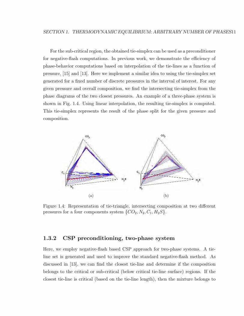
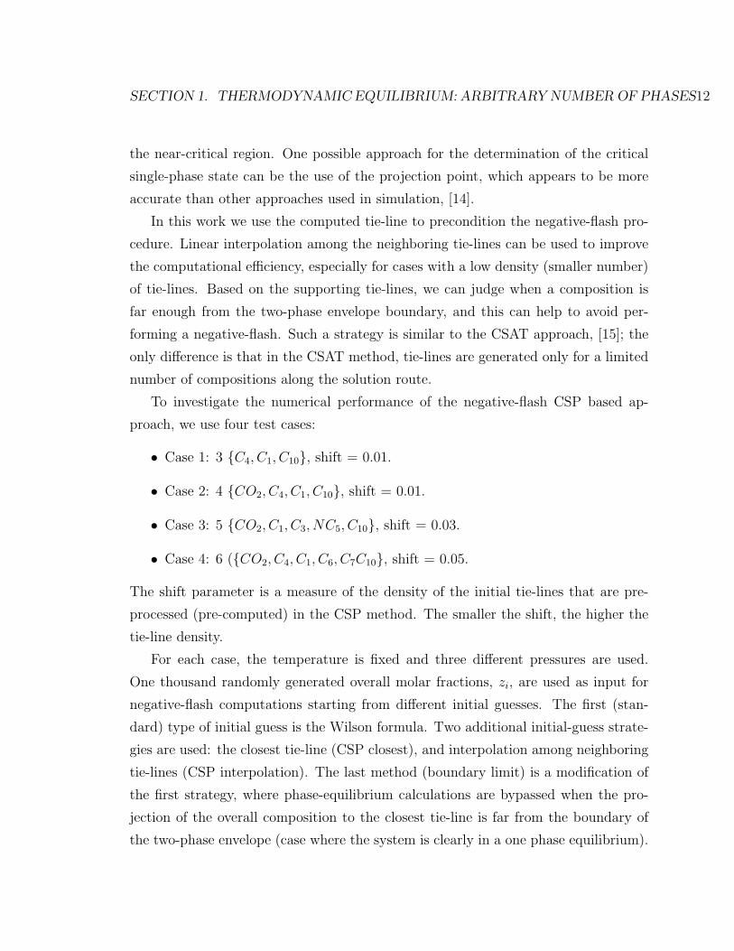
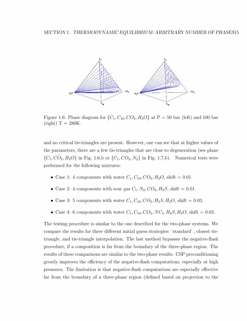
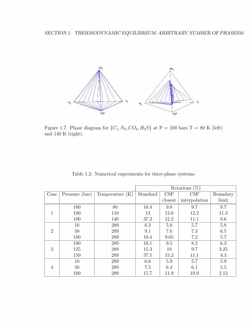
SECTION 1. THERMODYNAMIC EQUILIBRIUM: ARBITRARY NUMBER OF PHASES17
supporting tie-triangle), and that makes CSP preconditioning a very efficient method
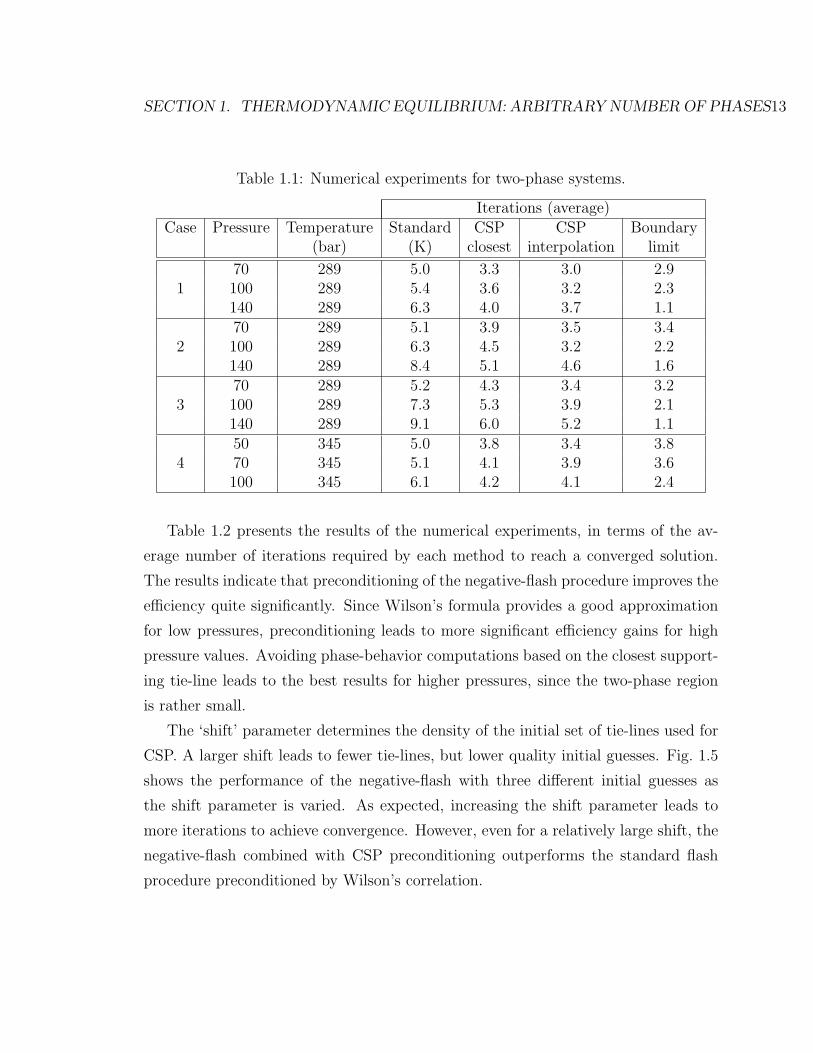
for high-pressure systems.
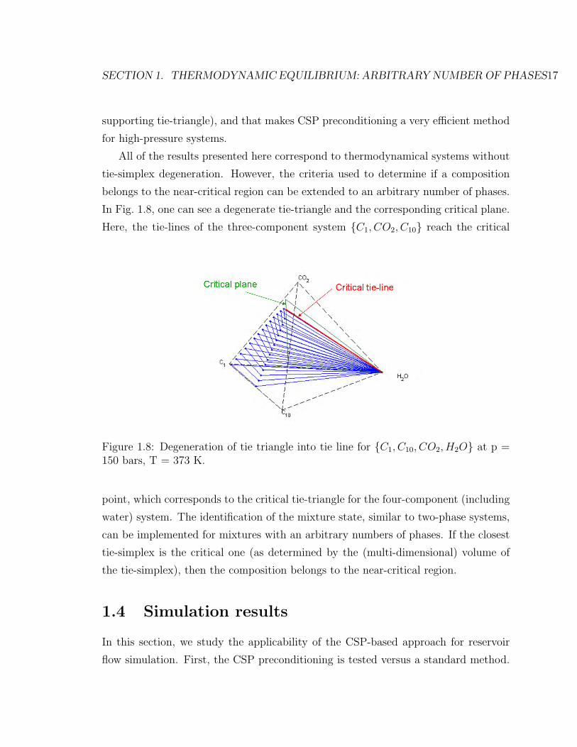
All of the results presented here correspond to thermodynamical systems without
tie-simplex degeneration. However, the criteria used to determine if a composition
belongs to the near-critical region can be extended to an arbitrary number of phases.
In Fig. 1.8, one can see a degenerate tie-triangle and the corresponding critical plane.
Here, the tie-lines of the three-component system C1, CO2, C10 reach the critical
Figure 1.8: Degeneration of tie triangle into tie line for C1, C10, CO2, H2O at p =150 bars, T = 373 K.
point, which corresponds to the critical tie-triangle for the four-component (including
water) system. The identification of the mixture state, similar to two-phase systems,
can be implemented for mixtures with an arbitrary numbers of phases. If the closest
tie-simplex is the critical one (as determined by the (multi-dimensional) volume of
the tie-simplex), then the composition belongs to the near-critical region.
1.4 Simulation results
In this section, we study the applicability of the CSP-based approach for reservoir
flow simulation. First, the CSP preconditioning is tested versus a standard method.
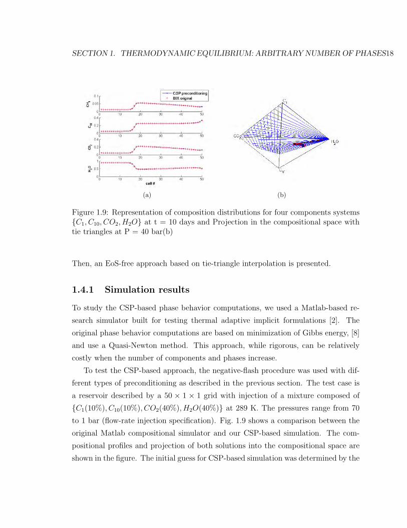
SECTION 1. THERMODYNAMIC EQUILIBRIUM: ARBITRARY NUMBER OF PHASES18
(a) (b)
Figure 1.9: Representation of composition distributions for four components systemsC1, C10, CO2, H2O at t = 10 days and Projection in the compositional space withtie triangles at P = 40 bar(b)
Then, an EoS-free approach based on tie-triangle interpolation is presented.
1.4.1 Simulation results
To study the CSP-based phase behavior computations, we used a Matlab-based re-
search simulator built for testing thermal adaptive implicit formulations [2]. The
original phase behavior computations are based on minimization of Gibbs energy, [8]
and use a Quasi-Newton method. This approach, while rigorous, can be relatively
costly when the number of components and phases increase.
To test the CSP-based approach, the negative-flash procedure was used with dif-
ferent types of preconditioning as described in the previous section. The test case is
a reservoir described by a 50 × 1 × 1 grid with injection of a mixture composed of
C1(10%), C10(10%), CO2(40%), H2O(40%) at 289 K. The pressures range from 70
to 1 bar (flow-rate injection specification). Fig. 1.9 shows a comparison between the
original Matlab compositional simulator and our CSP-based simulation. The com-
positional profiles and projection of both solutions into the compositional space are
shown in the figure. The initial guess for CSP-based simulation was determined by the
SECTION 1. THERMODYNAMIC EQUILIBRIUM: ARBITRARY NUMBER OF PHASES19
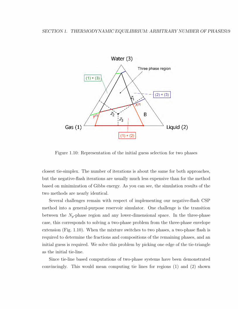
Figure 1.10: Representation of the initial guess selection for two phases
closest tie-simplex. The number of iterations is about the same for both approaches,
but the negative-flash iterations are usually much less expensive than for the method
based on minimization of Gibbs energy. As you can see, the simulation results of the
two methods are nearly identical.
Several challenges remain with respect of implementing our negative-flash CSP
method into a general-purpose reservoir simulator. One challenge is the transition
between the Np-phase region and any lower-dimensional space. In the three-phase
case, this corresponds to solving a two-phase problem from the three-phase envelope
extension (Fig. 1.10). When the mixture switches to two phases, a two-phase flash is
required to determine the fractions and compositions of the remaining phases, and an
initial guess is required. We solve this problem by picking one edge of the tie-triangle
as the initial tie-line.
Since tie-line based computations of two-phase systems have been demonstrated
convincingly. This would mean computing tie lines for regions (1) and (2) shown
SECTION 1. THERMODYNAMIC EQUILIBRIUM: ARBITRARY NUMBER OF PHASES20
in Fig. 1.10. However, Fig. 1.10 represents a ternary diagram with constant K-
values. In real cases, super-critical effects may appear and the two-phase envelope
may degenerate into a point (see Fig. 1.3).
1.4.2 EoS-free approach
One of the advantages of the CSP approach is the possibility to avoid EoS related
computations during a simulation run, since the pre-computed tie-simplex set provides
a parameterization of the compositional space. Tie-simplex interpolation provides a
continuous description of the entire compositional space, not only as a function of
pressure, but also as a function of the tie-simplex parameter, γ. Even when the
density of the tie-simplex set is small, the precision of linear interpolation among the
tie-simplexes is usually quite good. In previous work, [15], the efficiency of the EoS-
free approach was demonstrated for tie-line parameterization; here we demonstrate
it for tie-triangles.
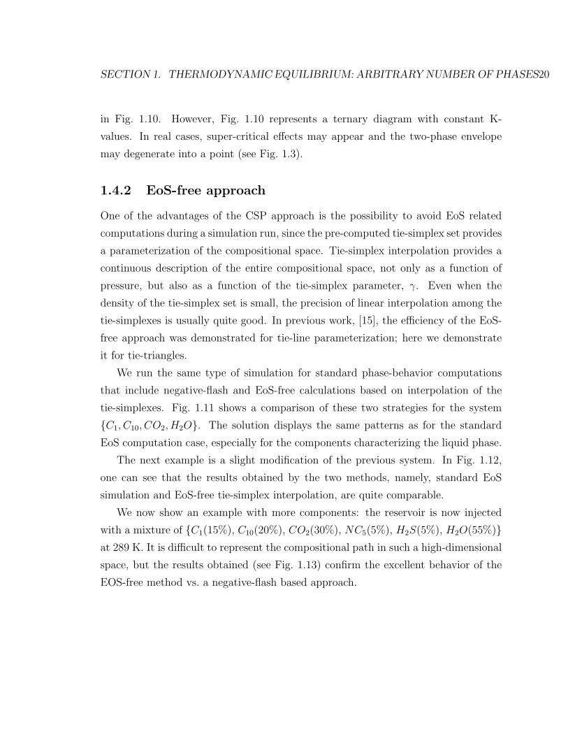
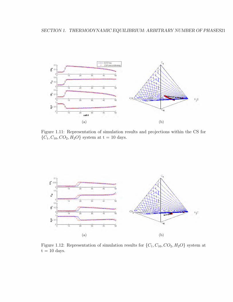
We run the same type of simulation for standard phase-behavior computations
that include negative-flash and EoS-free calculations based on interpolation of the
tie-simplexes. Fig. 1.11 shows a comparison of these two strategies for the system
C1, C10, CO2, H2O. The solution displays the same patterns as for the standard
EoS computation case, especially for the components characterizing the liquid phase.
The next example is a slight modification of the previous system. In Fig. 1.12,
one can see that the results obtained by the two methods, namely, standard EoS
simulation and EoS-free tie-simplex interpolation, are quite comparable.
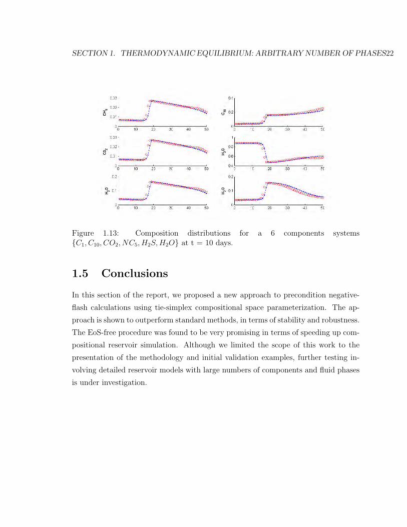
We now show an example with more components: the reservoir is now injected
with a mixture of C1(15%), C10(20%), CO2(30%), NC5(5%), H2S(5%), H2O(55%)at 289 K. It is difficult to represent the compositional path in such a high-dimensional
space, but the results obtained (see Fig. 1.13) confirm the excellent behavior of the
EOS-free method vs. a negative-flash based approach.
SECTION 1. THERMODYNAMIC EQUILIBRIUM: ARBITRARY NUMBER OF PHASES21
(a) (b)
Figure 1.11: Representation of simulation results and projections within the CS forC1, C10, CO2, H2O system at t = 10 days.
(a) (b)
Figure 1.12: Representation of simulation results for C1, C10, CO2, H2O system att = 10 days.
SECTION 1. THERMODYNAMIC EQUILIBRIUM: ARBITRARY NUMBER OF PHASES22
Figure 1.13: Composition distributions for a 6 components systemsC1, C10, CO2, NC5, H2S,H2O at t = 10 days.
1.5 Conclusions
In this section of the report, we proposed a new approach to precondition negative-
flash calculations using tie-simplex compositional space parameterization. The ap-
proach is shown to outperform standard methods, in terms of stability and robustness.
The EoS-free procedure was found to be very promising in terms of speeding up com-
positional reservoir simulation. Although we limited the scope of this work to the
presentation of the methodology and initial validation examples, further testing in-
volving detailed reservoir models with large numbers of components and fluid phases
is under investigation.
Bibliography
[1] Firoozabadi A. Thermodynamics of Hydrocarbon Reservoirs. New York, NY:
McGraw-Hill, 1999.
[2] Tchelepi H. Agarwal A., Moncorge A. Criteria for the thermal adaptive im-
plicit method. SPE Annual Technical Conference and Exhibition, (SPE 103060),
September 2006. held in San Antonio, Texas.
[3] K. Aziz and A. Settari. Petroleum Reservoir Simulation. Applied Science Pub-
lishers, 1979.
[4] K. Aziz and T.W. Wong. Considerations in the development of multipurpose
reservoir simulation models. Proceedings of the 1st and 2nd International Forum
on Reservoir Simulation, September 1988-1989.
[5] Voskov D.V. Entov V.M., Turetskaya F.D. On approximation of phase equilibria
of multicomponent hydrocarbon mixtures and prediction of oil displacement by
gas injection. 8th European Conference on the Mathematics of Oil Recovery,
Freiburg, Germany, September 2001.
[6] Rasmussen C.P. Krejbjerg K. Michelsen M.L. Bjurstrom K.E. Increasing of
computational speed of flash calculations with applications for compositional,
transient simulations. SPE REE, February 2006.
[7] Y.K. Li and L.X. Nghiem. The development of a general phase envelope construc-
tion algorithm for reservoir fluid studies. 57th Annual Fall Technical Conference
and Exhibition, New Orleans, (SPE Paper 11198), September 1982.
23
BIBLIOGRAPHY 24
[8] M.L. Michelsen and J.M. Mollerup. Thermodynamic Models: Fundamentals and
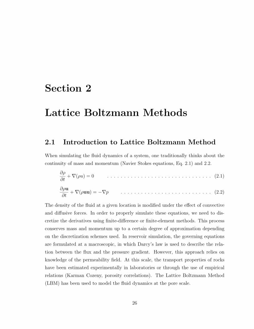
The density of the fluid at a given location is modified under the effect of convective
and diffusive forces. In order to properly simulate these equations, we need to dis-
cretize the derivatives using finite-difference or finite-element methods. This process
conserves mass and momentum up to a certain degree of approximation depending
on the discretization schemes used. In reservoir simulation, the governing equations
are formulated at a macroscopic, in which Darcy’s law is used to describe the rela-
tion between the flux and the pressure gradient. However, this approach relies on
knowledge of the permeability field. At this scale, the transport properties of rocks
have been estimated experimentally in laboratories or through the use of empirical
relations (Karman Cozeny, porosity correlations). The Lattice Boltzmann Method
(LBM) has been used to model the fluid dynamics at the pore scale.
26
SECTION 2. LATTICE BOLTZMANN METHODS 27
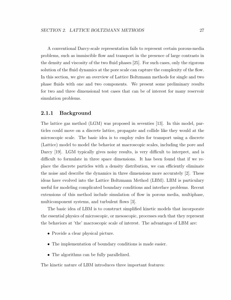
A conventional Darcy-scale representation fails to represent certain porous-media
problems, such as immiscible flow and transport in the presence of large contrasts in
the density and viscosity of the two fluid phases [25]. For such cases, only the rigorous
solution of the fluid dynamics at the pore scale can capture the complexity of the flow.
In this section, we give an overview of Lattice Boltzmann methods for single and two
phase fluids with one and two components. We present some preliminary results
for two and three dimensional test cases that can be of interest for many reservoir
simulation problems.
2.1.1 Background
The lattice gas method (LGM) was proposed in seventies [13]. In this model, par-
ticles could move on a discrete lattice, propagate and collide like they would at the
microscopic scale. The basic idea is to employ rules for transport using a discrete
(Lattice) model to model the behavior at macroscopic scales, including the pore and
Darcy [19]. LGM typically gives noisy results, is very difficult to interpret, and is
difficult to formulate in three space dimensions. It has been found that if we re-
place the discrete particles with a density distribution, we can efficiently eliminate
the noise and describe the dynamics in three dimensions more accurately [2]. These
ideas have evolved into the Lattice Boltzmann Method (LBM). LBM is particulary
useful for modeling complicated boundary conditions and interface problems. Recent
extensions of this method include simulation of flow in porous media, multiphase,
multicomponent systems, and turbulent flows [3].
The basic idea of LBM is to construct simplified kinetic models that incorporate
the essential physics of microscopic, or mesoscopic, processes such that they represent
the behaviors at ’the’ macroscopic scale of interest. The advantages of LBM are:
• Provide a clear physical picture.
• The implementation of boundary conditions is made easier.
• The algorithms can be fully parallelized.
The kinetic nature of LBM introduces three important features:
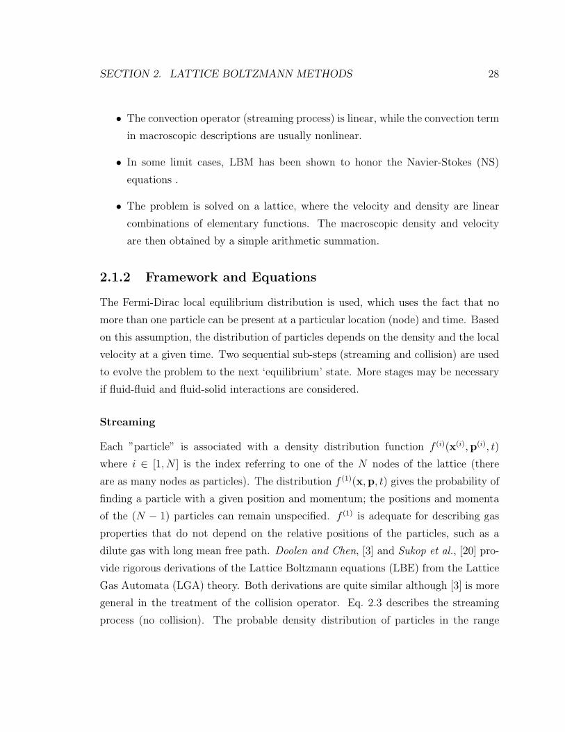
SECTION 2. LATTICE BOLTZMANN METHODS 28
• The convection operator (streaming process) is linear, while the convection term
in macroscopic descriptions are usually nonlinear.
• In some limit cases, LBM has been shown to honor the Navier-Stokes (NS)
equations .
• The problem is solved on a lattice, where the velocity and density are linear
combinations of elementary functions. The macroscopic density and velocity
are then obtained by a simple arithmetic summation.
2.1.2 Framework and Equations
The Fermi-Dirac local equilibrium distribution is used, which uses the fact that no
more than one particle can be present at a particular location (node) and time. Based
on this assumption, the distribution of particles depends on the density and the local
velocity at a given time. Two sequential sub-steps (streaming and collision) are used
to evolve the problem to the next ‘equilibrium’ state. More stages may be necessary
if fluid-fluid and fluid-solid interactions are considered.
Streaming
Each ”particle” is associated with a density distribution function f (i)(x(i),p(i), t)
where i ∈ [1, N ] is the index referring to one of the N nodes of the lattice (there
are as many nodes as particles). The distribution f (1)(x,p, t) gives the probability of
finding a particle with a given position and momentum; the positions and momenta
of the (N − 1) particles can remain unspecified. f (1) is adequate for describing gas
properties that do not depend on the relative positions of the particles, such as a
dilute gas with long mean free path. Doolen and Chen, [3] and Sukop et al., [20] pro-
vide rigorous derivations of the Lattice Boltzmann equations (LBE) from the Lattice
Gas Automata (LGA) theory. Both derivations are quite similar although [3] is more
general in the treatment of the collision operator. Eq. 2.3 describes the streaming
process (no collision). The probable density distribution of particles in the range
SECTION 2. LATTICE BOLTZMANN METHODS 29
x + dx with momentum p + dp is f (1)(x,p, t)dxdp
f (1)(x + dx,p + dp, t+ dt) = f (1)(x,p, t)dxdp (2.3)
The linearization of the streaming step is quite straightforward, since the probability
density distribution at a given time depends only on the state of the system at the
previous time. The introduction of collisions makes the problem nonlinear and more
difficult to solve.
Collision
Let Γ(−)dxdpdt be the number of molecules (particles) that do not reach the expected
portion of the phase space (x,p) due to collisions, and Γ(+)dxdpdt be the number of
molecules that start from somewhere other than (x,p) and arrive in that portion of
space due to collisions.
f (1)(x + dx,p + dp, t+ dt)dxdp =
f (1)(x,p, t)dxdp +[Γ(+) − Γ(−)
]dxdpdt (2.4)
Boltzmann’s equation is derived from a first-order Taylor series expansion of Eq. 2.4.
f (1)(x + dx,p + dp, t+ dt) =
f (1)(x,p, t) + dx.∇xf(1) + dp.∇pf
(1) +
(∂f (1)
∂t
)dt+ . . . (2.5)
We replace the left member in Eq. 2.4. We obtain Boltzmann’s equation, Eq. 2.6[f (1)(x,p, t) + dx.∇xf
(1) + dp.∇pf(1) +
(∂f (1)
∂t
)dt+ . . .
]dxdp =
f (1)(x,p, t)dxdp +[Γ(+) − Γ(−)
]dxdpdt (2.6)
We approximately solve Eq. 2.6. We first introduce the discretized mesh that is used
to solve the system.
Macroscopic scale
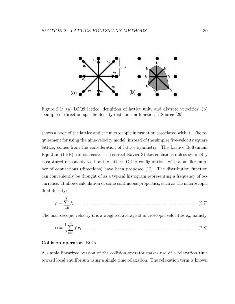
Particle positions are confined to the nodes of the lattice. Eight directions, three mag-
nitudes, and one particle mass define what is called the D2Q9 lattice [29]. Fig. 2.1
SECTION 2. LATTICE BOLTZMANN METHODS 30
Figure 2.1: (a) D2Q9 lattice, definition of lattice unit, and discrete velocities; (b)example of direction specific density distribution function f. Source [29].
shows a node of the lattice and the microscopic information associated with it. The re-
quirement for using the nine-velocity model, instead of the simpler five-velocity square
lattice, comes from the consideration of lattice symmetry. The Lattice Boltzmann
Equation (LBE) cannot recover the correct Navier-Stokes equations unless symmetry
is captured reasonably well by the lattice. Other configurations with a smaller num-
ber of connections (directions) have been proposed [12]. The distribution function
can conveniently be thought of as a typical histogram representing a frequency of oc-
currence. It allows calculation of some continuous properties, such as the macroscopic
where a b c and d are lattice constants. This expansion is valid only for small velocities,
or small Mach numbers u/Cs , where Cs is the speed of sound. If we use the constraint
in Eq. 2.8, we obtain the coefficients of Eq. 2.10.
f eqi (x) = wiρ(x)
[1 + 3
ei.u
c2+
9
2
(ei.u)2
c4− 3
2
u2
c2
]. . . . . . . . . . . . (2.11)
Where the weights wi are 4/9 for particle (i = 0), 1/9 for i = 1, 2, 3, 4 and 1/36 for
i = 5, 6, 7, 8. Here, c is the basic celerity of the lattice.
Bounce-back boundaries
LBM’s ability to solve flow problems for any type of boundary condition provides a
clear advantage over other discretization approaches. This is due to the inherently
local character of LBM based descriptions. Interactions between fluid and solid are
resolved at the boundary and involve the set of particles that are directly in contact
with the ‘walls’ in the system. We separate the solid into two types: boundary solids
SECTION 2. LATTICE BOLTZMANN METHODS 32
that lie at the solid-fluid interface and isolated solids that do not contact the fluid.
With this division it is possible to eliminate unnecessary computations at inactive
nodes. Indeed, the volume occupied by immobile particles do not need to be included
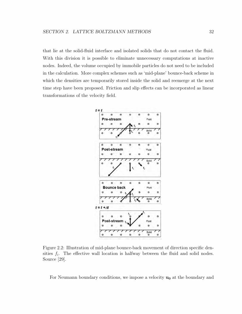
in the calculation. More complex schemes such as ‘mid-plane’ bounce-back scheme in
which the densities are temporarily stored inside the solid and reemerge at the next
time step have been proposed. Friction and slip effects can be incorporated as linear
transformations of the velocity field.
Figure 2.2: Illustration of mid-plane bounce-back movement of direction specific den-sities fi. The effective wall location is halfway between the fluid and solid nodes.Source [29].
For Neumann boundary conditions, we impose a velocity u0 at the boundary and
SECTION 2. LATTICE BOLTZMANN METHODS 33
use equations 2.8. Fig. 2.2 shows the decomposition of a bounce-back collision. Here,
we solve the system
ρ0 = f1 + f2 + f3 + f4 + f5 + f6 + f7 + f8
0 = f1 − f3 + f5 − f6 − f7 + f8
ρ0v = f2 − f4 + f6 − f7 − f8
f4 − f eq4 = f2 − f eq2 (2.12)
in order to find the remaining density distribution functions. For Dirichlet bound-
ary conditions, we use an Equation of State (EoS) of type P = RTρ to relate the
density and pressure. Then, we use the same equation to find the velocity, and then
calculate the macroscopic variables. Chapter 4.4 and 4.5 of Sukop [20] give a detailed
description of the system of equations 2.12.
2.2 Single Component Single Phase, SCSP
We begin with a single phase fluid featuring only one component. This scenario is
the starting point of several publications, [29], [21], [12]. We implemented many of
these methods in Matlab simulator in order to study various flow settings and better
understand the jump from a particle based representation to newtonian fluid prop-
erties. One important element concerns the boundary condition. The pressure needs
to decrease along the flow direction; otherwise, unphysical results may be obtained.
Then the pressure and density are related via an EoS of the type P = C2sρ = ρ/3
(Fig. 2.6). This transition is essential in order to relate microscopic, statistical data
(particles velocities, probability distribution) to a macroscopic description of the fluid
(density, velocity). One starts with a non-dimensional head gradient, convert to a real
world pure pressure gradient, compute the Reynolds number and define an equivalent
LBM system. We rarely mention the Reynolds number in flow in natural porous-
media. Here, it is reintroduced since it gives information about the size of particles
in comparison with the characteristic length of the system via the global velocity. As
mentioned previously, we do not solve a real microscopic problem since the number
of particles to consider would be prohibitively large. Instead, we solve the problem
SECTION 2. LATTICE BOLTZMANN METHODS 34
using particles of intermediate size (mesoscopic). The gap between these scales has
to be bridged through assumptions on the collision operator. Cases with too few par-
ticles result in high Reynolds numbers that cannot be dealt with easily. Some rules
of thumb concerning an appropriate number of particles are drawn from heuristic
considerations [26].
The LBM algorithm for single-phase flow is as follows:
1. Calculate the local density, momentum and stress using Eq. 2.7, 2.8.
2. Calculate the post-collision distribution (collision step).
3. Apply a force according to the pressure gradient ∇P .
4. Move the distribution to the neighboring nodes (propagation step).
5. Repeat (1)-(4) until a steady state is reached.
An external force (gravity) is implemented as a perturbation of the density distribu-
tion after collision. The no-slip boundary condition is implemented using the bounce-
back scheme. There is a no-flow boundary condition perpendicular to the pressure
gradient. Periodic boundary conditions are imposed at the inlet and outlet.
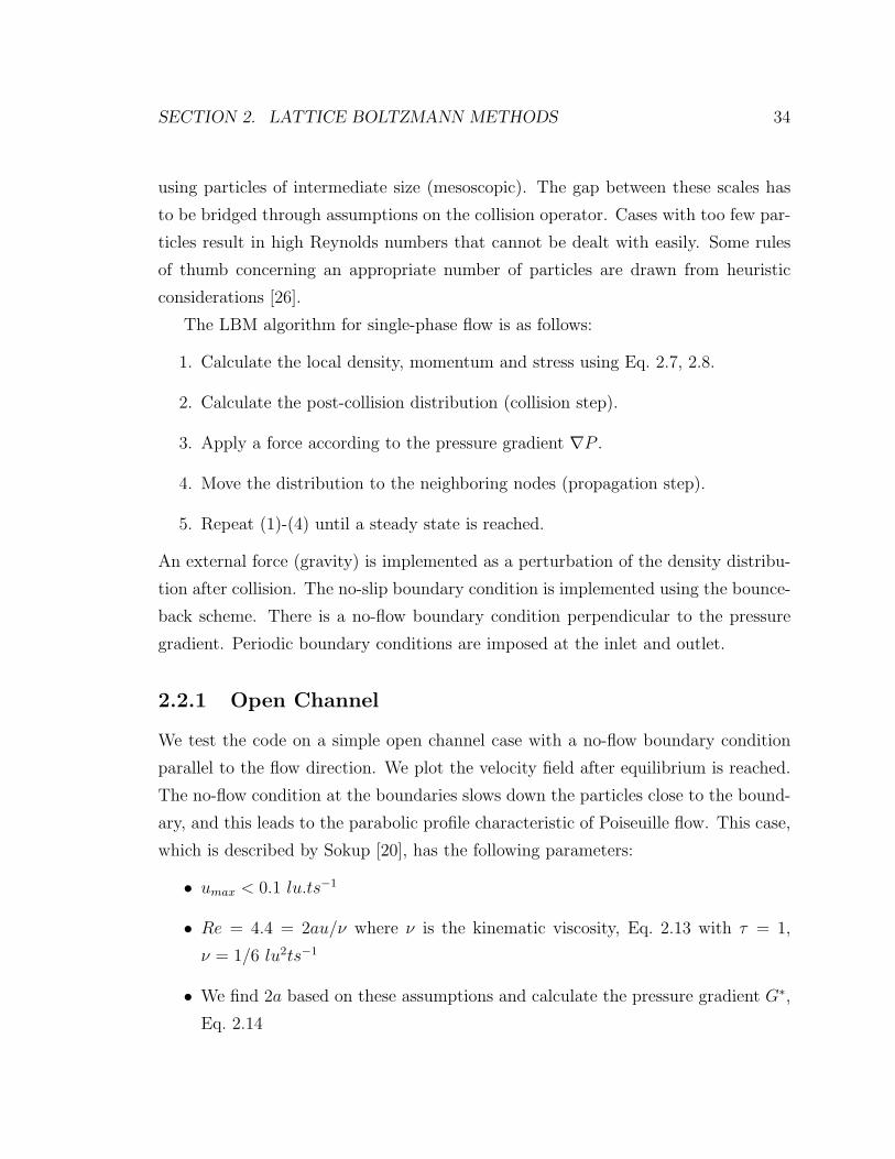
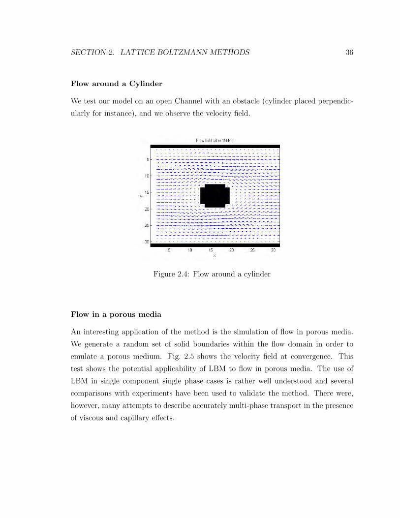
2.2.1 Open Channel
We test the code on a simple open channel case with a no-flow boundary condition
parallel to the flow direction. We plot the velocity field after equilibrium is reached.
The no-flow condition at the boundaries slows down the particles close to the bound-
ary, and this leads to the parabolic profile characteristic of Poiseuille flow. This case,
which is described by Sokup [20], has the following parameters:
• umax < 0.1 lu.ts−1
• Re = 4.4 = 2au/ν where ν is the kinematic viscosity, Eq. 2.13 with τ = 1,
ν = 1/6 lu2ts−1
• We find 2a based on these assumptions and calculate the pressure gradient G∗,
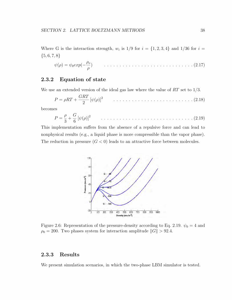
This implementation suffers from the absence of a repulsive force and can lead to
nonphysical results (e.g., a liquid phase is more compressible than the vapor phase).
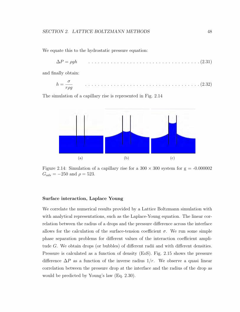
The reduction in pressure (G < 0) leads to an attractive force between molecules.
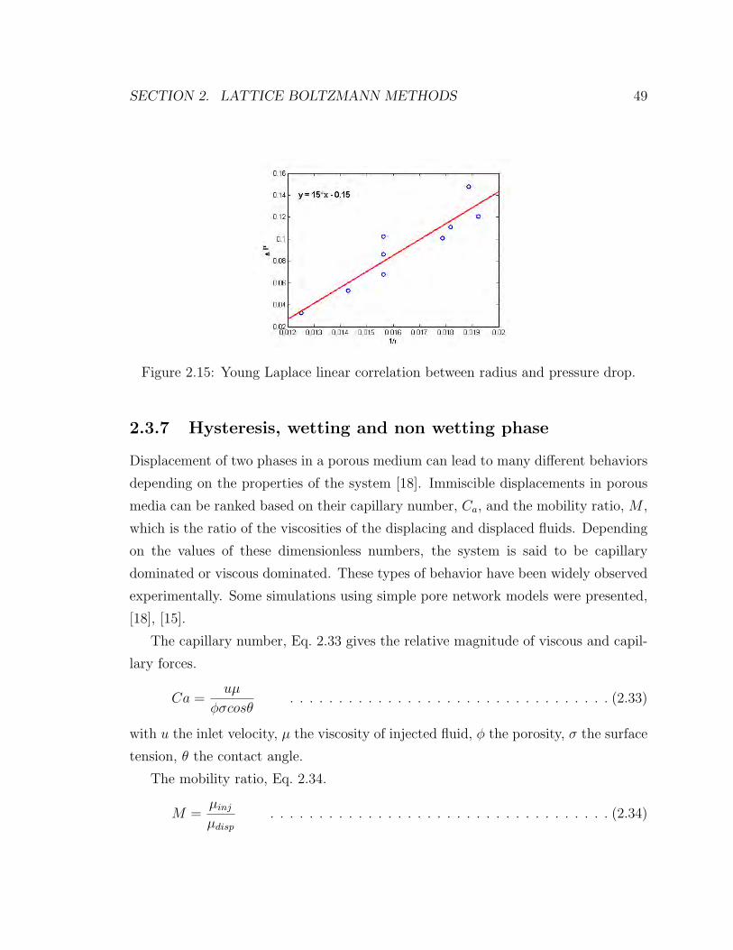
Figure 2.6: Representation of the pressure-density according to Eq. 2.19. ψ0 = 4 andρ0 = 200. Two phases system for interaction amplitude ‖G‖ > 92.4.
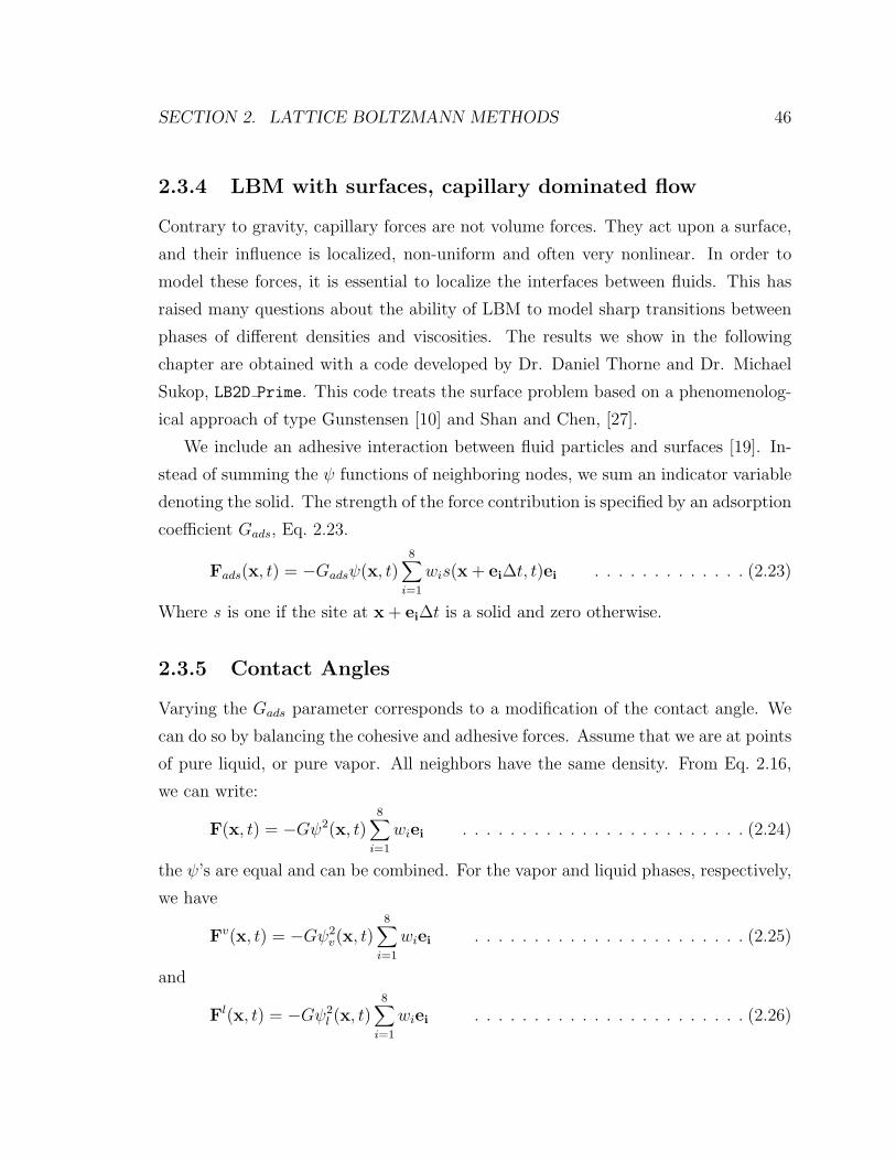
2.3.3 Results
We present simulation scenarios, in which the two-phase LBM simulator is tested.
SECTION 2. LATTICE BOLTZMANN METHODS 39
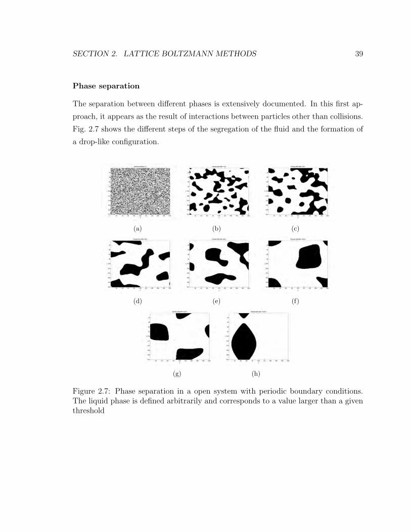
Phase separation
The separation between different phases is extensively documented. In this first ap-
proach, it appears as the result of interactions between particles other than collisions.
Fig. 2.7 shows the different steps of the segregation of the fluid and the formation of
a drop-like configuration.
(a) (b) (c)
(d) (e) (f)
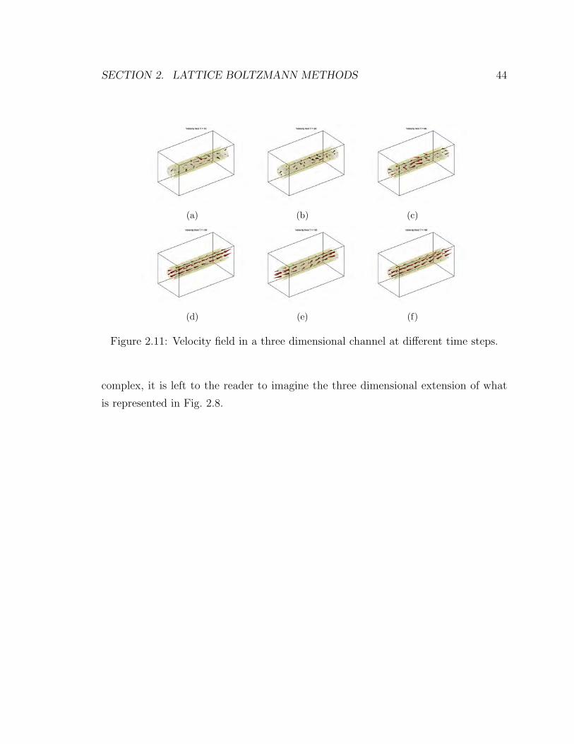
(g) (h)
Figure 2.7: Phase separation in a open system with periodic boundary conditions.The liquid phase is defined arbitrarily and corresponds to a value larger than a giventhreshold
SECTION 2. LATTICE BOLTZMANN METHODS 40
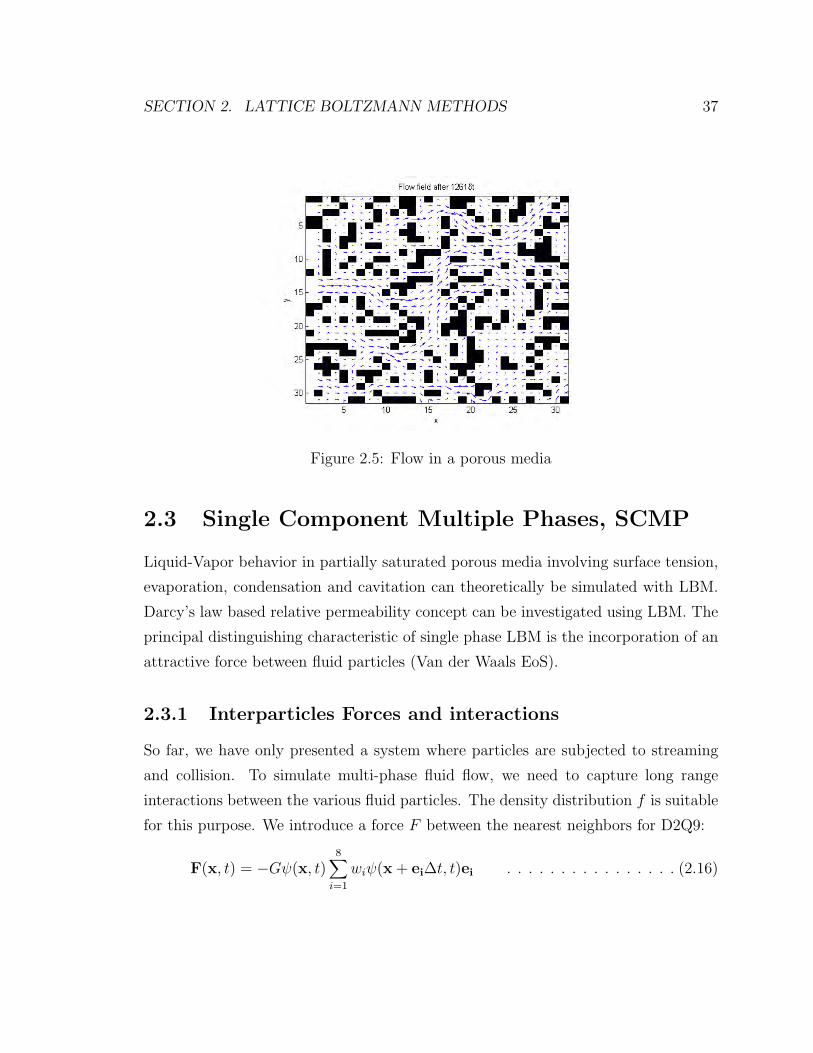
Porous media Flow without capillary effects
The boundary-condition treatment raises several questions. In the code implementa-
tion used here, our attempts to introduce a particle-solid interaction were not success-
ful. The introduction of a surface tension requires the computation of an interface.
The position of this interface depends on the force balance, which is a function of the
surface tension. This nonlinear problem may be overcome by modifying the collision
operator. However, the literature on this topic does not point in one overall direction,
and a reference method has not been clearly established yet. We were able to simulate
some effects, such as the apparition of contact angles and curved interfaces. However,
the convergence in a case where we clearly define an interface between two fluids was
not achieved. The reason for this is associated with a time-scale constraint. The flow
problem considered here is doubly transient. The first transient period relates to the
statistical nature of the microscopic information and the fact that the information is
propagated locally from one node to its direct neighbors. As a consequence, the sys-
tem needs time to reach a steady state in the Boltzmann sense. There is also a second
transient period due to the dynamics of the system at the macroscale (e.g., compress-
ibility). This results in a time constraint comparable to a CFL number. When the
two characteristic times are of the same order, such as in regions close to an interface
where the density gradient induces an acceleration of particles, the system becomes
unstable. This effect has been reported by several authors, [9], [21] and reveals one of
the limitations of the single relaxation-time proposed by the Bhatnagar-Gross-Krook
(Eq. 2.9) model.
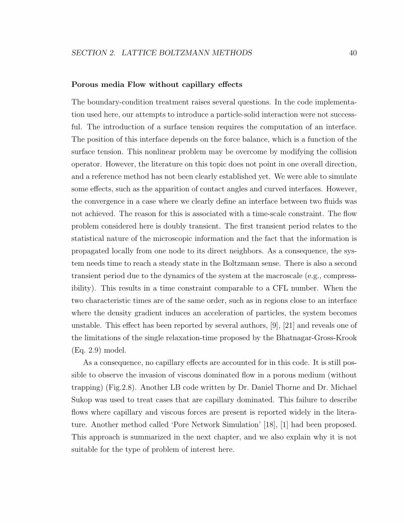
As a consequence, no capillary effects are accounted for in this code. It is still pos-
sible to observe the invasion of viscous dominated flow in a porous medium (without
trapping) (Fig.2.8). Another LB code written by Dr. Daniel Thorne and Dr. Michael
Sukop was used to treat cases that are capillary dominated. This failure to describe
flows where capillary and viscous forces are present is reported widely in the litera-
ture. Another method called ‘Pore Network Simulation’ [18], [1] had been proposed.
This approach is summarized in the next chapter, and we also explain why it is not
suitable for the type of problem of interest here.
SECTION 2. LATTICE BOLTZMANN METHODS 41
(a) (b) (c)
(d)
Figure 2.8: Density distribution over time in a porous media. Capillary effects arehere neglected and no boundaries are accounted for at the edges.
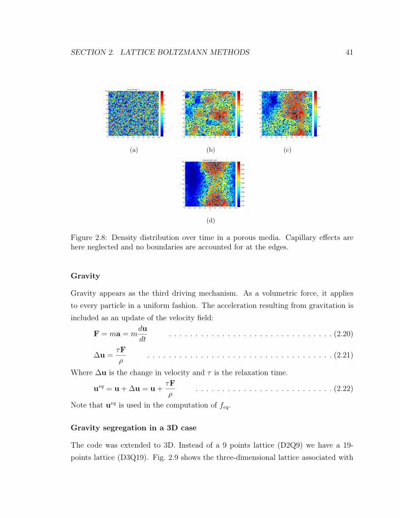
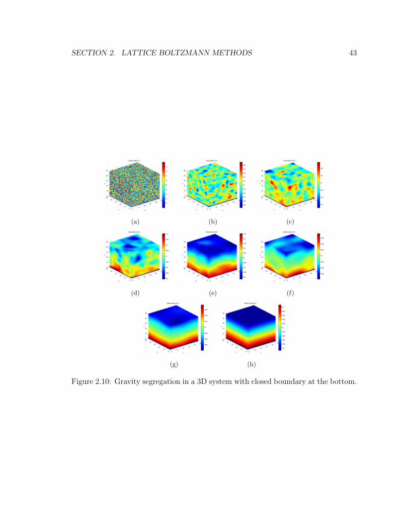
Gravity
Gravity appears as the third driving mechanism. As a volumetric force, it applies
to every particle in a uniform fashion. The acceleration resulting from gravitation is
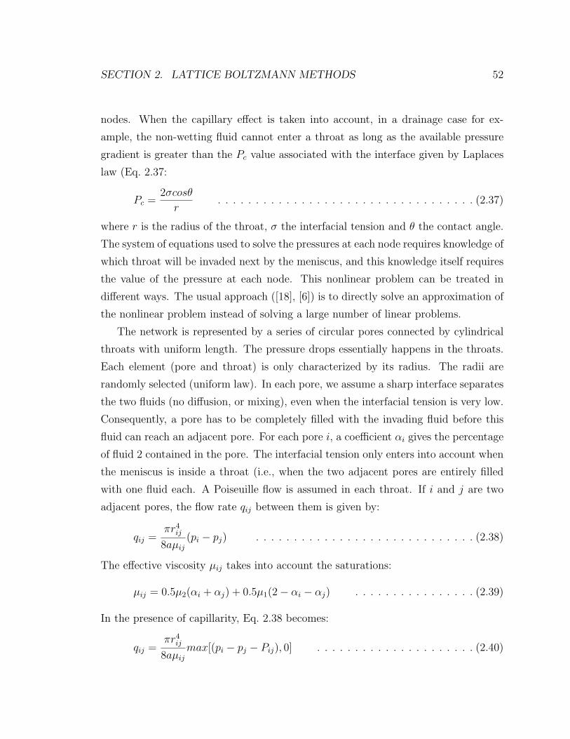
This means that there is no flow between i and j as long as the pressure difference is
lower than the pressure necessary for the invasion of the pore (Eq. 2.37).
The flow between two interfacial nodes no longer depends linearly on the pressure
difference: the flow is zero up to a threshold value. The solution of this nonlinear
problem is approached through a relaxation technique. At each time step, the network
is swept several times, updating the pressure at each node from the pressure of its
neighbors through the flow-conservation equation (the flow is taken to be zero between
two interfacial nodes as long as the pressure threshold is not reached). Once the
computations arrive at a stable numerical state, the simulation stops. At this stage,
the total flow rate and the contents of each pore are known. The time step is then
calculated as the time required to completely fill one pore. This means that the
interface is moved in all the pores until it reaches a throat.
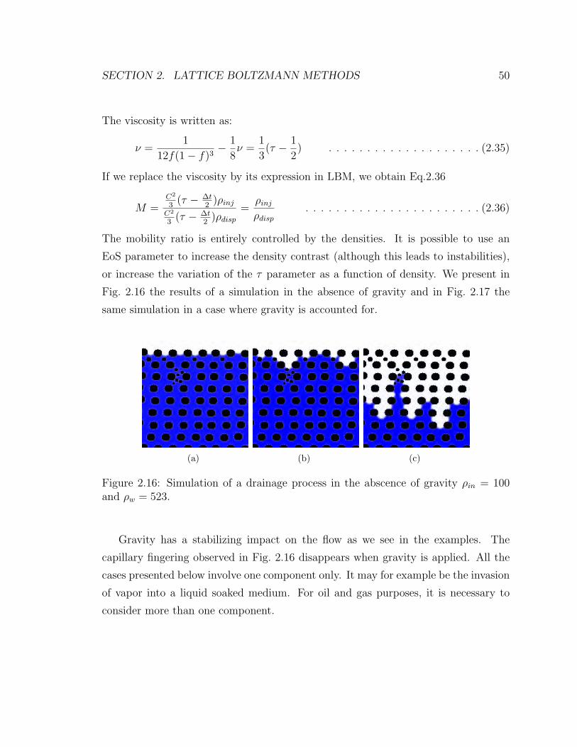
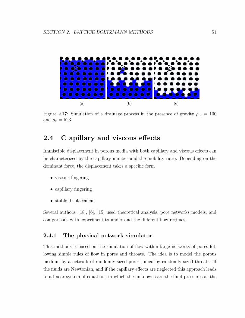
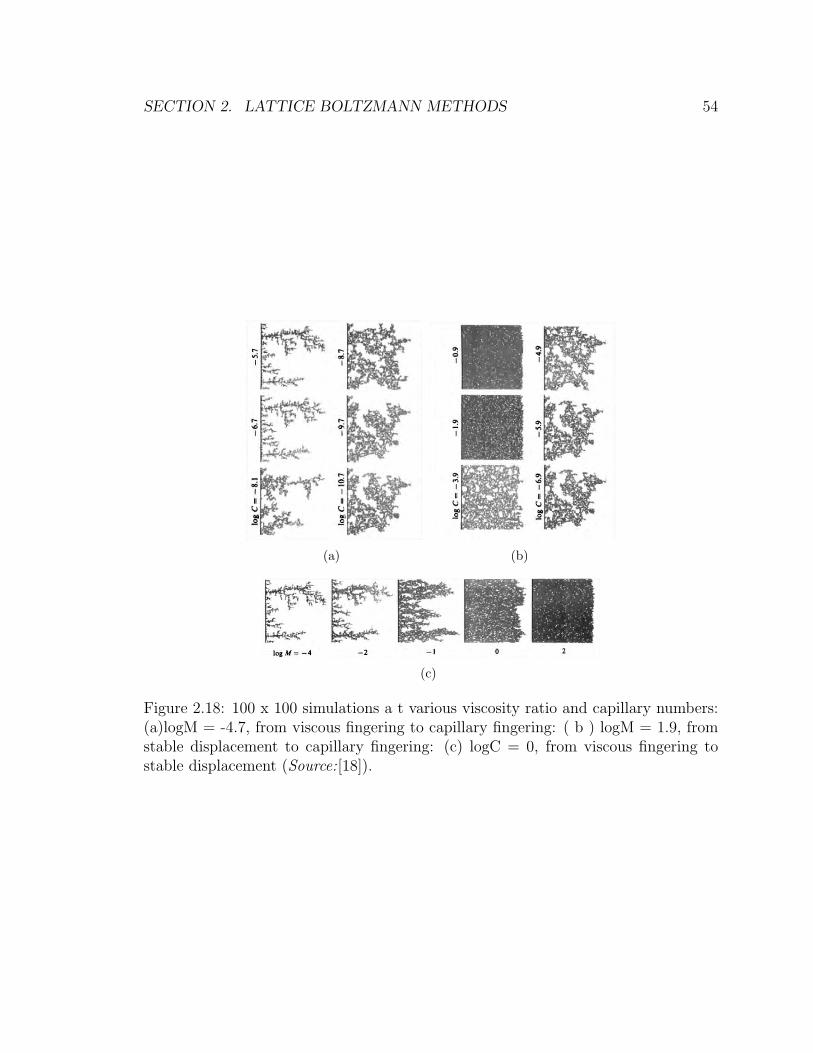
2.4.2 Phase diagram
The three modes of displacement are compared based on two numbers: the mobility
ratio M and the capillary number C. The regimes are:
1. Stable displacement : the principal force is due to the viscosity of the injected
fluid; capillary effects and pressure drop in the displaced fluid are negligible,
Fig. 2.18 (b) logC = −0.9.
2. Viscous fingering : the principal force is due to the viscosity of the displaced
fluid; capillary effects and pressure drop in the displacing fluid are negligible.
The tree-like fingers have no loops. They spread across the whole network and
they grow towards the exit, Fig. 2.18 (a) logC = −5.7
3. Capillary fingering : at low capillary number, the viscous forces are negligible in
both fluids and the principal force is due to capillarity. The fingers also spread
across the network but the pattern is different from the previous case and the
final saturation is larger. At all scales, the fingers grow in all directions, even
backward (toward the entrance). They form loops which trap the displaced
SECTION 2. LATTICE BOLTZMANN METHODS 54
(a) (b)
(c)
Figure 2.18: 100 x 100 simulations a t various viscosity ratio and capillary numbers:(a)logM = -4.7, from viscous fingering to capillary fingering: ( b ) logM = 1.9, fromstable displacement to capillary fingering: (c) logC = 0, from viscous fingering tostable displacement (Source:[18]).
SECTION 2. LATTICE BOLTZMANN METHODS 55
fluid. The size of the trapped clusters range from the pore size to macroscopic
scales, of the order of the network size, Fig. 2.18 (a), logC = −10.7.
2.5 LBM simulation of multi-component, multi-
phase flows
Lattice-gas models of phase separation have been reviewed by several authors, [26], [3].
Three main implementations have been proposed over the past fifteen years. These
are the Gunstensen [10], Shan and Chen [27], and the Free Energy [24], [23] models.
In these methods, various schemes are used to identify the interface and compute a
collision operator that can model phase separations in cases where different types of
particles are interacting.
In the method of Gunstensen et al. [10], [7], [8], red and blue particle distribution
functions f ri (x, t) and f bi (x, t) are introduced to represent the two different fluids. The
total particle distribution function (or the color-blind particle distribution function)
is defined as: fi = f ri (x, t) + f bi (x, t). The LBM equation is written for each phase:
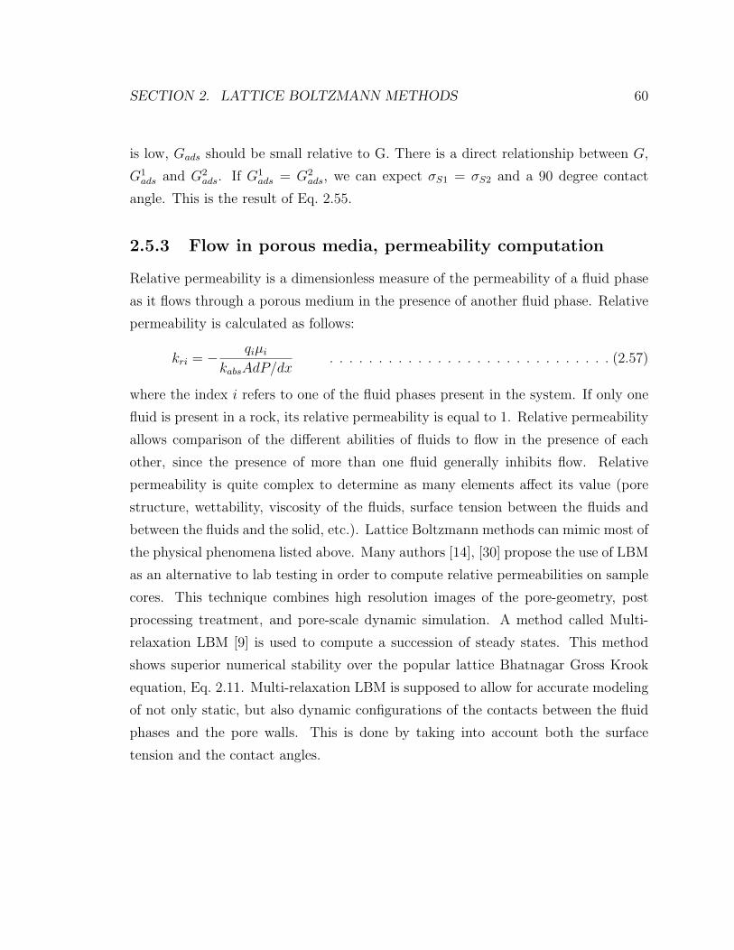
where the index i refers to one of the fluid phases present in the system. If only one
fluid is present in a rock, its relative permeability is equal to 1. Relative permeability
allows comparison of the different abilities of fluids to flow in the presence of each
other, since the presence of more than one fluid generally inhibits flow. Relative
permeability is quite complex to determine as many elements affect its value (pore
structure, wettability, viscosity of the fluids, surface tension between the fluids and
between the fluids and the solid, etc.). Lattice Boltzmann methods can mimic most of
the physical phenomena listed above. Many authors [14], [30] propose the use of LBM
as an alternative to lab testing in order to compute relative permeabilities on sample
cores. This technique combines high resolution images of the pore-geometry, post
processing treatment, and pore-scale dynamic simulation. A method called Multi-
relaxation LBM [9] is used to compute a succession of steady states. This method
shows superior numerical stability over the popular lattice Bhatnagar Gross Krook
equation, Eq. 2.11. Multi-relaxation LBM is supposed to allow for accurate modeling
of not only static, but also dynamic configurations of the contacts between the fluid
phases and the pore walls. This is done by taking into account both the surface
tension and the contact angles.
SECTION 2. LATTICE BOLTZMANN METHODS 61
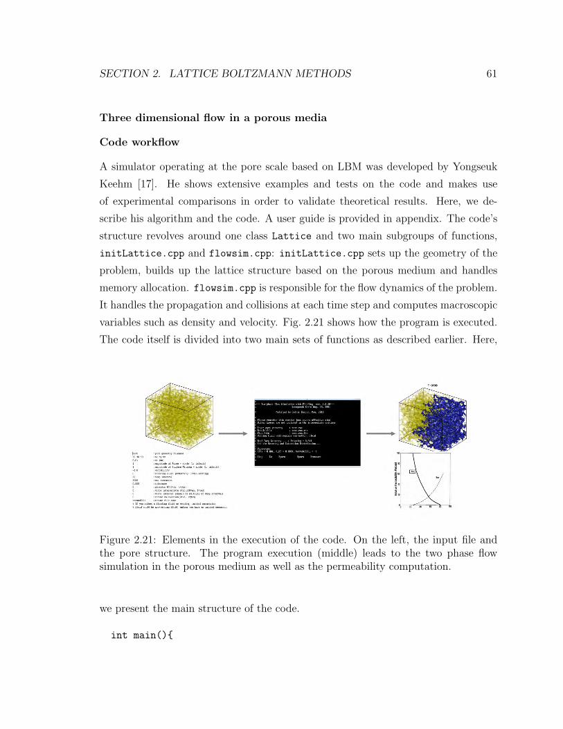
Three dimensional flow in a porous media
Code workflow
A simulator operating at the pore scale based on LBM was developed by Yongseuk
Keehm [17]. He shows extensive examples and tests on the code and makes use
of experimental comparisons in order to validate theoretical results. Here, we de-
scribe his algorithm and the code. A user guide is provided in appendix. The code’s
structure revolves around one class Lattice and two main subgroups of functions,
initLattice.cpp and flowsim.cpp: initLattice.cpp sets up the geometry of the
problem, builds up the lattice structure based on the porous medium and handles
memory allocation. flowsim.cpp is responsible for the flow dynamics of the problem.
It handles the propagation and collisions at each time step and computes macroscopic
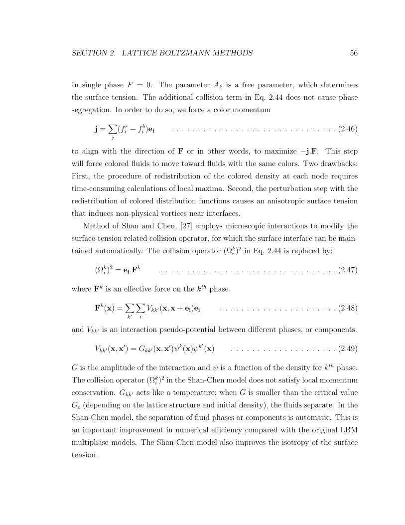
variables such as density and velocity. Fig. 2.21 shows how the program is executed.
The code itself is divided into two main sets of functions as described earlier. Here,
Figure 2.21: Elements in the execution of the code. On the left, the input file andthe pore structure. The program execution (middle) leads to the two phase flowsimulation in the porous medium as well as the permeability computation.
we present the main structure of the code.
int main()
SECTION 2. LATTICE BOLTZMANN METHODS 62
Lattice lat(’inputFile’);// Constructs the lattice based on input file parameter
lat.initLattice(); // Sets the geometry of the problem
lat.flowSim(); // Runs the 2-phase flow simulation
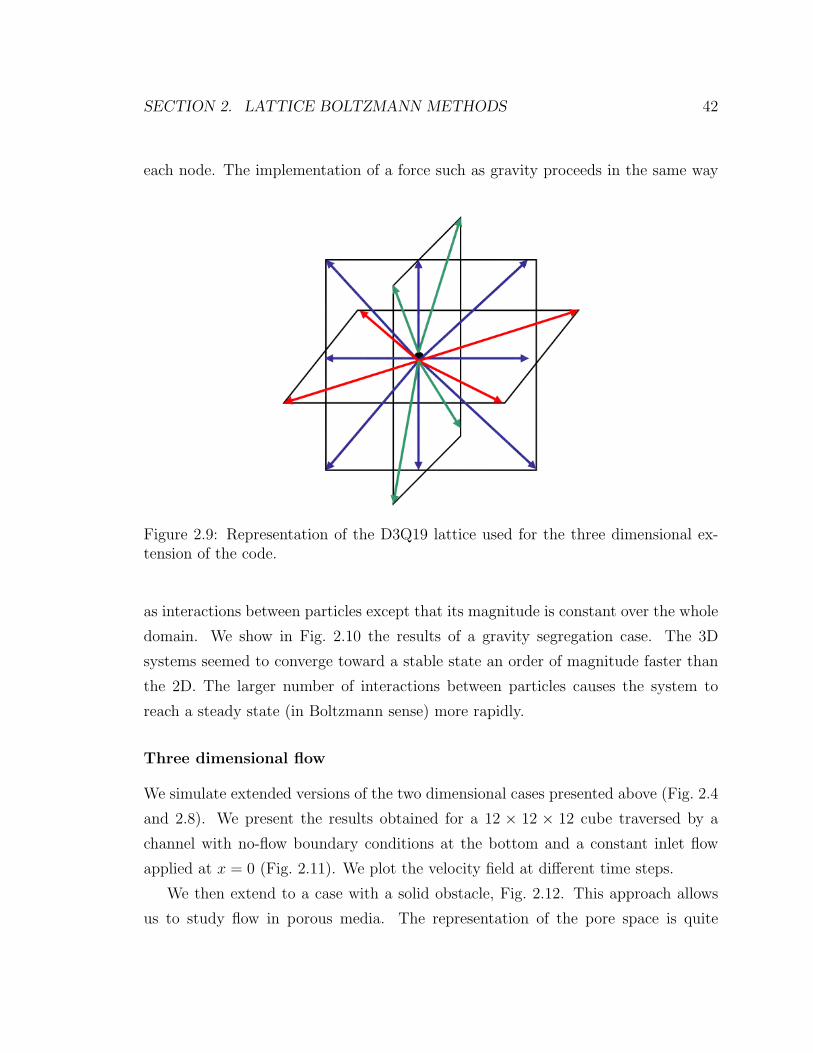
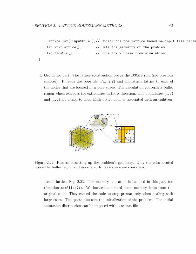
1. Geometric part: The lattice construction obeys the D3Q19 rule (see previous
chapter). It reads the pore file, Fig. 2.22 and allocates a lattice to each of
the nodes that are located in a pore space. The calculation concerns a buffer
region which excludes the extremities in the x direction. The boundaries (x, z)
and (x, z) are closed to flow. Each active node is associated with an eighteen-
Figure 2.22: Process of setting up the problem’s geometry. Only the cells locatedinside the buffer region and associated to pore space are considered.
stencil lattice, Fig. 2.23. The memory allocation is handled in this part too
(function memAlloc()). We located and fixed some memory leaks from the
original code. They caused the code to stop prematurely when dealing with
large cases. This parts also sees the initialization of the problem. The initial
saturation distribution can be imposed with a restart file.
SECTION 2. LATTICE BOLTZMANN METHODS 63
Figure 2.23: Lattice structure and indexing chosen in the code.
SECTION 2. LATTICE BOLTZMANN METHODS 64
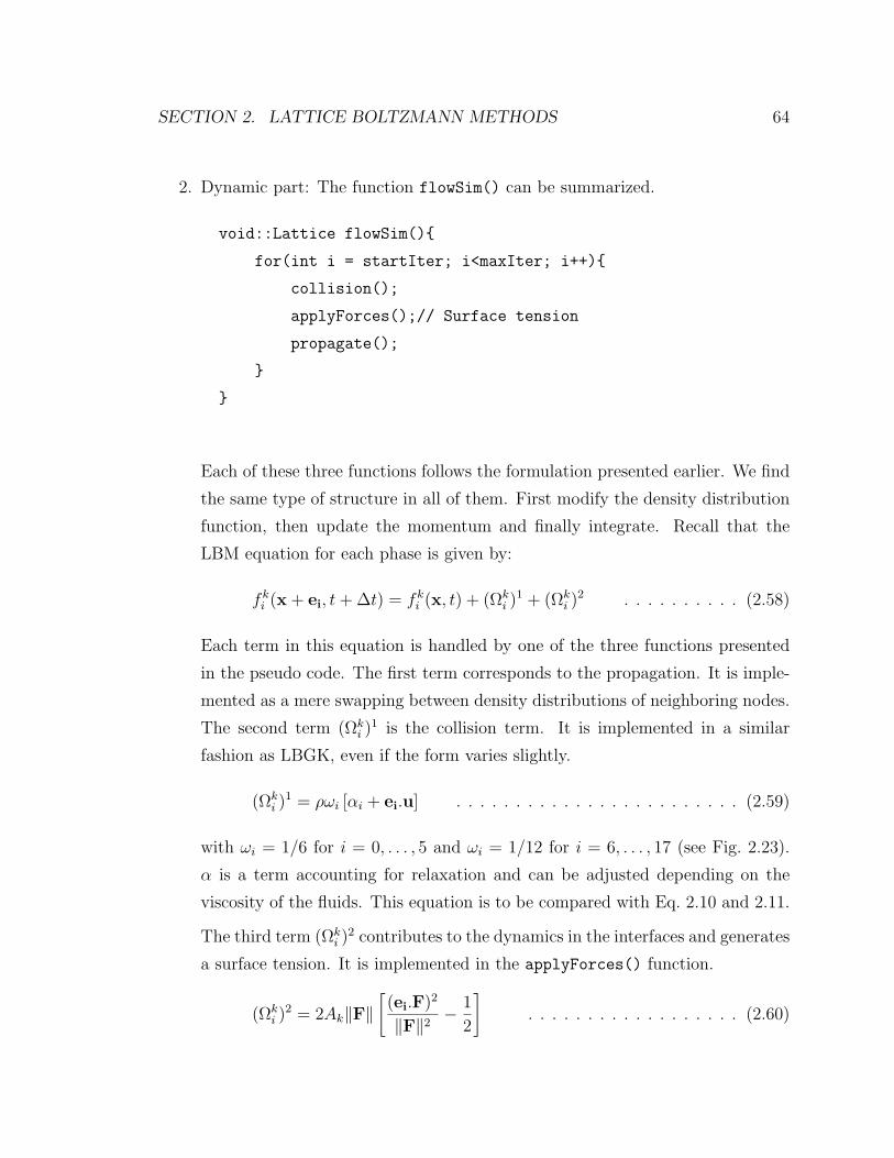
2. Dynamic part: The function flowSim() can be summarized.
void::Lattice flowSim()
for(int i = startIter; i<maxIter; i++)
collision();
applyForces();// Surface tension
propagate();
Each of these three functions follows the formulation presented earlier. We find
the same type of structure in all of them. First modify the density distribution
function, then update the momentum and finally integrate. Recall that the
LBM equation for each phase is given by:
fki (x + ei, t+ ∆t) = fki (x, t) + (Ωki )
1 + (Ωki )
2 . . . . . . . . . . (2.58)
Each term in this equation is handled by one of the three functions presented
in the pseudo code. The first term corresponds to the propagation. It is imple-
mented as a mere swapping between density distributions of neighboring nodes.
The second term (Ωki )
1 is the collision term. It is implemented in a similar
fashion as LBGK, even if the form varies slightly.
The function maxST() ranks the node by order of highest gradient and updates
the density distribution following Eq. 2.59. The density distributions are up-
dated (as well as the color gradient), and we stop applying forces when the
gradient becomes very small.
The simulation stops when the code reaches the maximum number of iterations,
or when the system reaches a steady state. Convergence is established when the
new computed flow is close to the one calculated from the previous time step. The
convergence ratios (ratioR and ratioB) are not computed at every time step. Instead
they are updated every time the program outputs results.
Examples
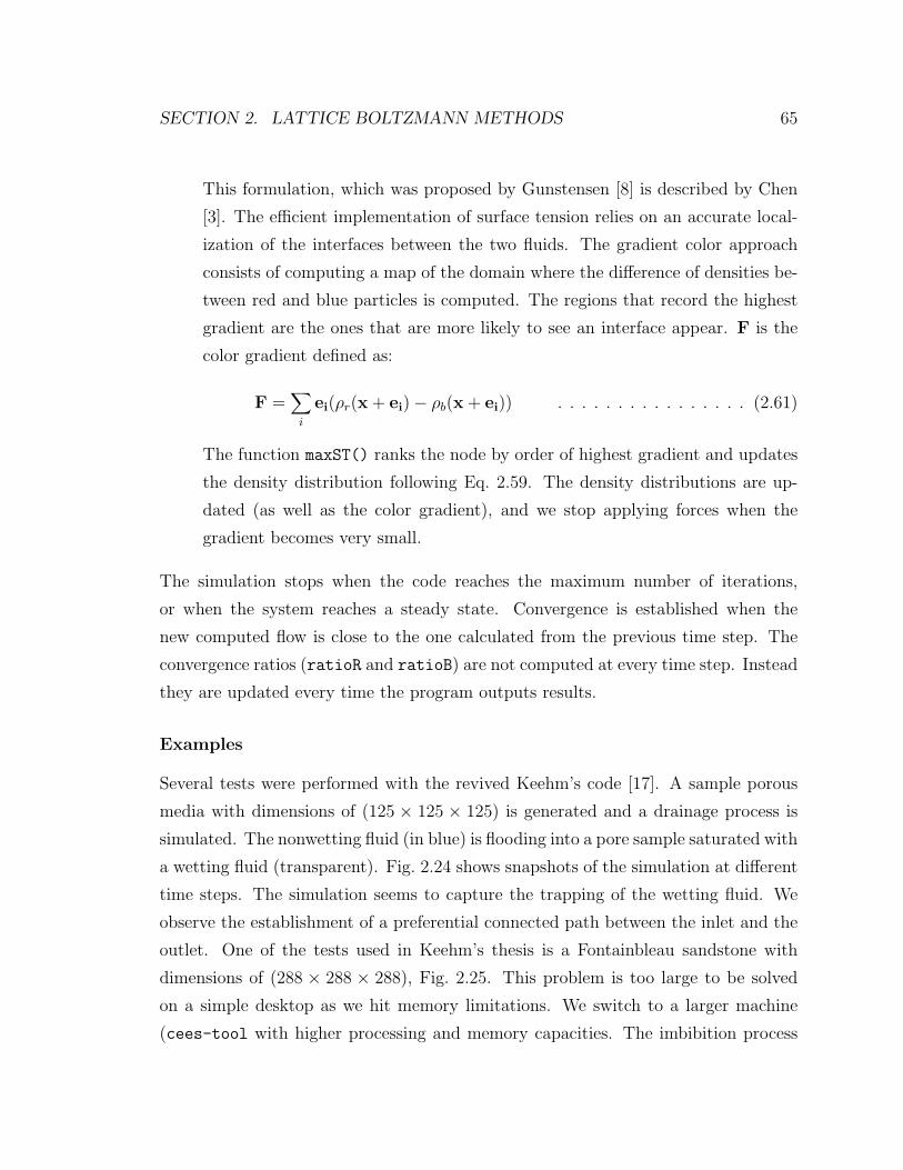
Several tests were performed with the revived Keehm’s code [17]. A sample porous
media with dimensions of (125 × 125 × 125) is generated and a drainage process is
simulated. The nonwetting fluid (in blue) is flooding into a pore sample saturated with
a wetting fluid (transparent). Fig. 2.24 shows snapshots of the simulation at different
time steps. The simulation seems to capture the trapping of the wetting fluid. We
observe the establishment of a preferential connected path between the inlet and the
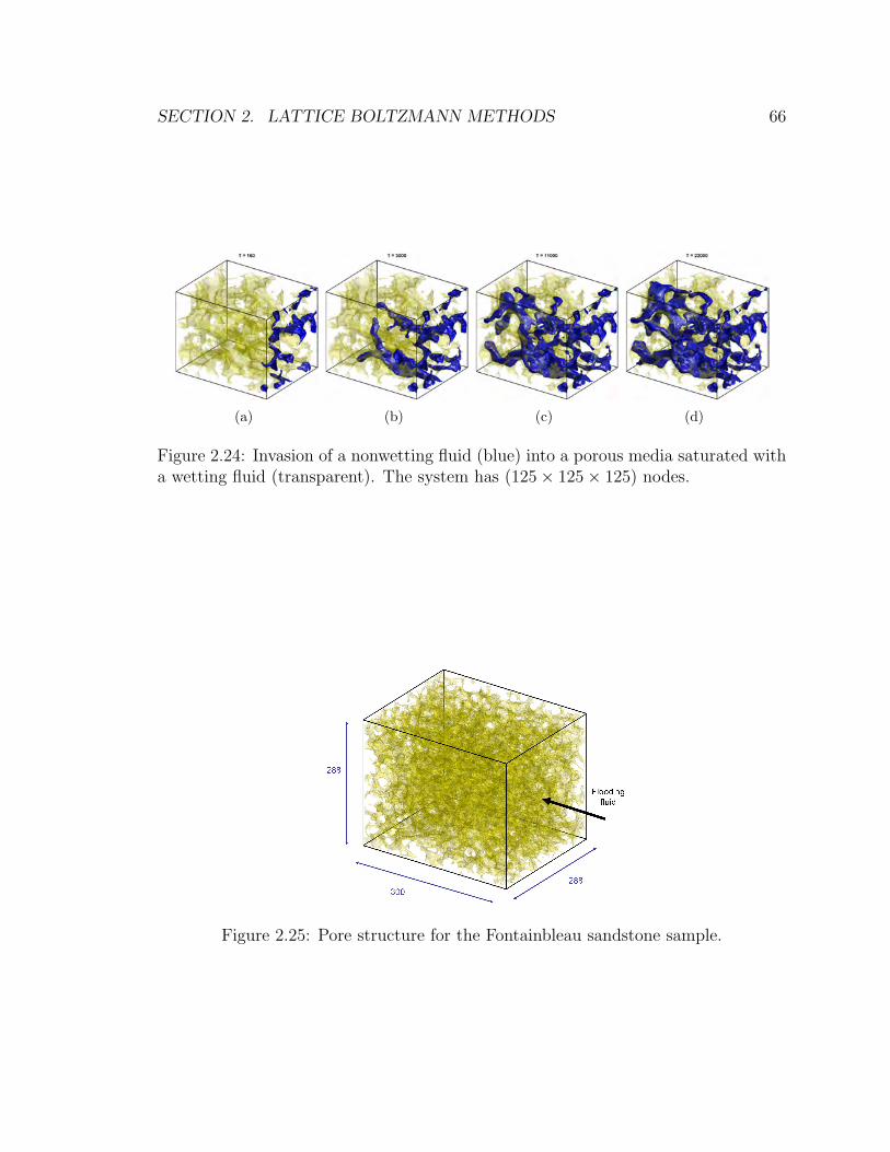
outlet. One of the tests used in Keehm’s thesis is a Fontainbleau sandstone with
dimensions of (288 × 288 × 288), Fig. 2.25. This problem is too large to be solved
on a simple desktop as we hit memory limitations. We switch to a larger machine
(cees-tool with higher processing and memory capacities. The imbibition process
SECTION 2. LATTICE BOLTZMANN METHODS 66
(a) (b) (c) (d)
Figure 2.24: Invasion of a nonwetting fluid (blue) into a porous media saturated witha wetting fluid (transparent). The system has (125× 125× 125) nodes.
Figure 2.25: Pore structure for the Fontainbleau sandstone sample.
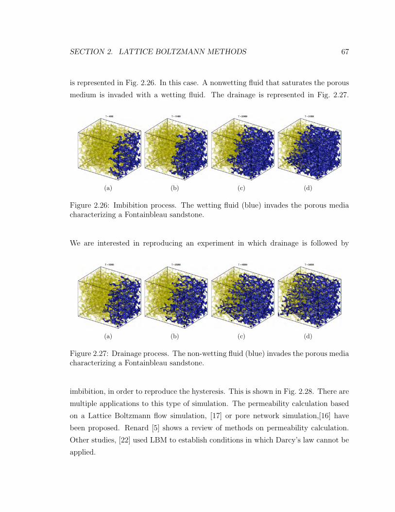
SECTION 2. LATTICE BOLTZMANN METHODS 67
is represented in Fig. 2.26. In this case. A nonwetting fluid that saturates the porous
medium is invaded with a wetting fluid. The drainage is represented in Fig. 2.27.
(a) (b) (c) (d)
Figure 2.26: Imbibition process. The wetting fluid (blue) invades the porous mediacharacterizing a Fontainbleau sandstone.
We are interested in reproducing an experiment in which drainage is followed by
(a) (b) (c) (d)
Figure 2.27: Drainage process. The non-wetting fluid (blue) invades the porous mediacharacterizing a Fontainbleau sandstone.
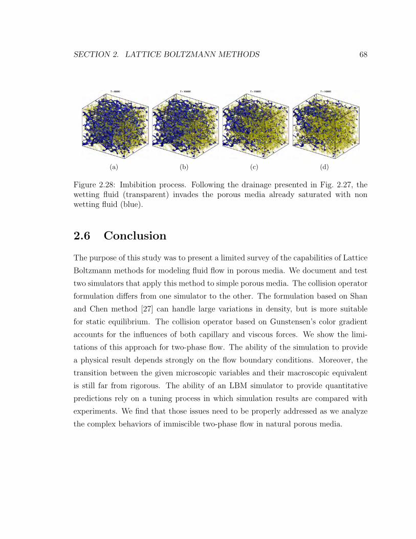
imbibition, in order to reproduce the hysteresis. This is shown in Fig. 2.28. There are
multiple applications to this type of simulation. The permeability calculation based
on a Lattice Boltzmann flow simulation, [17] or pore network simulation,[16] have
been proposed. Renard [5] shows a review of methods on permeability calculation.
Other studies, [22] used LBM to establish conditions in which Darcy’s law cannot be
applied.
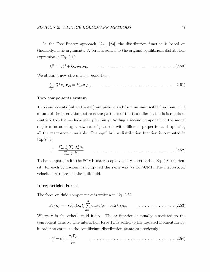
SECTION 2. LATTICE BOLTZMANN METHODS 68
(a) (b) (c) (d)
Figure 2.28: Imbibition process. Following the drainage presented in Fig. 2.27, thewetting fluid (transparent) invades the porous media already saturated with nonwetting fluid (blue).
2.6 Conclusion
The purpose of this study was to present a limited survey of the capabilities of Lattice
Boltzmann methods for modeling fluid flow in porous media. We document and test
two simulators that apply this method to simple porous media. The collision operator
formulation differs from one simulator to the other. The formulation based on Shan
and Chen method [27] can handle large variations in density, but is more suitable
for static equilibrium. The collision operator based on Gunstensen’s color gradient
accounts for the influences of both capillary and viscous forces. We show the limi-
tations of this approach for two-phase flow. The ability of the simulation to provide
a physical result depends strongly on the flow boundary conditions. Moreover, the
transition between the given microscopic variables and their macroscopic equivalent
is still far from rigorous. The ability of an LBM simulator to provide quantitative
predictions rely on a tuning process in which simulation results are compared with
experiments. We find that those issues need to be properly addressed as we analyze
the complex behaviors of immiscible two-phase flow in natural porous media.
Bibliography
[1] Pierre M. Adler and Howard Branner. Multiphase flow in porous media. Annual
Review Fluid Mechanics, 20:35–59, 1988.
[2] Chopard B. and Droz M. Cellular automata modeling of physical systems. Cam-
bridge Univeristy Press, page 341, 1998.
[3] Shiyi Chen and Gary D. Doolen. Lattice boltzmann method for fluid flow. Annual
Review Fluid Mechanics, 30(329-364), 1998.
[4] Romain de Loubens. Construction of High Order Adaptive Implicit Methods for
Reservoir Simulation. Department of Energy Resources Engineering Stanford
University, June 2007.
[5] Ph. Renard G. de Marsily. Calculating equivalent permeability: A review. Ad-
vances in Water Resources, 20(5), 1997.
[6] Cancelliere A. Chang C. Foti E. Rothman D.H. and Succi A. The permeability
of a random medium: Comparison of simulation with theory. Physics of Fluids,
A(2):2085–2088, 1990.
[7] Gunstensen A.K. Rothman D.H. Microscopic modeling of immiscible fluids in
three dimensions by a lattice boltzmann method. EPL (Europhysics Letters),
18(2):157–161, 1992.
[8] Gunstensen A.K. Rothman D.H. Lattice boltzmann studies of immiscible two
phase flow through porous media. Journal of Geophysical Research, 98(B4):6431–
6441, 1993.
69
BIBLIOGRAPHY 70
[9] Dominique dHumi‘eres Irina Ginzburg Manfred Krafczyk Pierre Lallemand and
Li-Shi Luo. Multiple-relaxation-time lattice boltzmann models in three dimen-
sions. The Royal Society, 360, February 2002.
[10] Gunstensen A.K. Rothman D.H. Zaleski S. Zanetti G. Lattice boltzmann model
of immiscible fluids. Physical Review A, 43(8):4320–4327, 1991.
[11] P. L. Bhatnagar E. P. Gross and M. Krook. A model for collision processes in
gases. small amplitude processes in charged and neutral one-component systems.
Physical Review, 94:511–525, 1954.
[12] Andrew K. Gunstensen. Lattice Boltzmann Studies of Multiphase Flow Through
Porous Media. Massachusetts Institute of Technology, June 1992.
[13] J. Hardy and Y. Pomeau. Microscopic model for viscous flow in two dimensions.
The American Physical society, (DOI: 10.1103/PhysRevA.16.720), 1976.
[14] Boaz Nur Amos Nur Jack Dvorkin Meghan Armbruster Chuck Baldwin Qian
Fang Naum Derzhi Carmen Gomez and Yaoming Mu. The future of rock physics:
Computational methods vs. lab testing. Ingrain, 2008.
[15] Che J.D. and D. Wilkinson. Pore-scale viscous fingering in porous media. Phys-
ical Review Letters, 55(18):1892–1895, 1985.
[16] Liping Jia. Reservoir Definition Through Integration of Multiscale Petrophysical
Data. Department of Energy Resources Engineering Stanford University, March
2005.
[17] Youngseuk Keehm. Computational Rock Physics: Transport Properties in Porous
Media and Applications. Department of Geophysics School of Earth Sciences
Stanford University, June 2003.
[18] Roland Lenormand and Eric Touboul. Numerical models and experiments on
immiscible displacements in porous media. Journal of Fluid Mechanics, 189:165–
187, 1988.
BIBLIOGRAPHY 71
[19] Nicos S. Martys and Hudong Chen. Simulation of multicomponent fluids in
complex three dimensional geometries by the lattice boltzmann method. The
American Physical society, 53(47.55.Mh), January 1996.
[20] Jr Michael C. Sukop, Daniel T. Thorne. Lattice Boltzmann Modeling. An Intro-
duction for Geoscientists and Engineers. Springer, krips bv edition, 2006.
[21] A. Kuzmin A.A. Mohamad. Multirange multi-relaxation time shan-chen model
with extended equilibrium. Computers and Mathematics with Applications, (El-
sevier), 2009.
[22] Dardis O. and McCloskey J. Lattice boltzmann scheme with real numbered
solid density for the simulation of flow in porous media. Physical Review E,
57(4):4834–4837, 1998.
[23] Michael R. Swift E. Orlandini W. R. Osborn and J. M. Yeomans. Lattice boltz-
mann simulations of liquid-gas and binary fluid systems. Physical Review E,
54(5), 1996.
[24] Michael R. Swift W. R. Osborn and J. M. Yeomans. Lattice boltzmann simula-
tion of nonideal fluids. Physical Review Letters, 75(5), 1995.
[25] Y. Cinar A. Riaz and H.A. Tchelepi. Experimental study of co2 injection into
saline formations. SPEJ, December 2009.
[26] Rothman D.H. Zaleski S. Lattice-gas models of phase separation: interfaces,
phase transitions and multiphase flow. Review Mod. Physics, (66):14171479,
1994.
[27] X. Shan and H. Chen. Lattice boltzmann model for simulating flows with multiple
phases and components. Physical Review E, 47(3), 1993.
[28] F. J. Higuera S. Succi and R. Benzi. Lattice gas dynamics with enhanced colli-