UCGE Reports Number 20254
Department of Geomatics Engineering
Improved Techniques for Measuring and Estimating Scaling Factors Used to Aggregate
Forest Transpiration (URL: http://www.geomatics.ucalgary.ca/research/publications/GradTheses.html)
by
María Rebeca Quiñonez-Piñón
March 2007
THE UNIVERSITY OF CALGARY
Improved Techniques for Measuring and Estimating
Scaling Factors Used to Aggregate Forest Transpiration
by
Marıa Rebeca Quinonez-Pinon
A DISSERTATION
SUBMITTED TO THE FACULTY OF GRADUATE STUDIES
IN PARTIAL FULFILLMENT OF THE REQUIREMENTS
FOR THE DEGREE OF DOCTOR OF PHILOSOPHY
DEPARTMENT OF GEOMATICS ENGINEERING
CALGARY, ALBERTA
MARCH, 2007
c© Marıa Rebeca Quinonez-Pinon 2007
Abstract
This research deals with transpiration scaling issues, and its aim is to improve five
boreal species canopy transpiration estimates that are computed by scaling up single
tree transpiration to the canopy scale. The improvement of canopy transpiration esti-
mates is made by developing a robust scaling approach. The robustness of the scaling
approach rests on fine input scaling parameter data and allometric regression models
developed at two different scales, tree and plot (i.e. canopy scale). Moreover, the scal-
ing approach integrates the habitat’s vegetation heterogeneity by developing regression
models for each species, and by adapting the scaling process to the particular allometric
characteristics of each species.
The scaling approach has three spatial scales: microscopic, tree, and plot. The
microscopic scale was used to accurately measure tree sapwood depth by means of
microscopical wood tissue analysis. Individual sapwood depth variations around the tree
trunk were also observed and quantified. There were interspecific allometric differences
showing that a tree’s sapwood area does not always grow as the tree grows. At the plot
scale, pure and mixed vascular vegetation plots of 60×60m and 10×10m were delimited.
Plot’s tree quantity and outside bark circumference at the breast height were recorded.
LAI was measured using the Tracing Radiation and Architecture of Canopies (TRAC)
and the LAI-2000 optical devices.
The results helped to generate the robust regression models. At the tree scale, re-
gression models were fitted between sapwood depth and outside bark diameter at the
breast height (DBHOB) to later estimate tree and plot sapwood area. However, not
all the models developed were linear relationships. Results for Pinus banksiana, Pinus
contorta, and Picea mariana did not lead to linear relationships, while results for Pop-
iii
iv
ulus tremuloides and Picea glauca did provide strong linear relationships. These results
prove that not all vascular species sapwood depth is directly proportional to their re-
spective DBHOB. Thus, two approaches to aggregate sapwood area to the plot scale
were combined. The new combined approach drew strong linear correlations at the plot
scale between sapwood area and leaf area. This last outcome conclusively proves the
theory claiming a linear correlation between sapwood area and leaf area at different
scales, where a lack of conclusive proof existed before.
The heat dissipation technique was used to collect diurnal tree sap flow and estimate
transpiration using sapwood area as the scaling parameter. Single tree sap flow was
aggregated to the plot scale using the plot’s sapwood area estimates. Since vegetation
transpiration rates vary among species, mixed forest transpiration is therefore influ-
enced by vegetation heterogeneity. Thus, the internal plot’s vegetation heterogeneity
was included in the scaling approach. Additionally, tree sap flow radial variations were
computed to provide a correction to in situ measurements. The final canopy transpi-
ration estimates were compared with the canopy actual evapotranspiration which was
estimated using the Penman-Monteith equation. Canopy transpiration was found to
be a large proportion of the canopy’s actual evapotranspiration, normally greater than
the 50%.
This improved scaling approach includes the error propagation estimation, and showed
that the error associated with a plot’s leaf area estimate increases with the plot size.
The error associated with tree and plot scale sapwood area estimates is practically null.
These demonstrate that the error associated with the biometrics can be significantly
minimized by using the most robust mensuration methods that currently exist.
Overall, the dissertation outcomes demonstrate that the use of robust methods and
the careful formulation of the scaling approach were fundamental in obtaining reliable
transpiration estimates. It is recommended that prior characterization of the intraspe-
cific biometrics variations be made in order to develop an adequate scaling approach.
Acknowledgements
This work was financially supported by several organizations. I thank for helping me to
accomplish this research The National Council of Science and Technology (CONACyT,
Mexico), the Center for Environmental Engineering Research and Education (CEERE,
U of C), the Metropolitan University (UAM, Mexico), Alberta Ingenuity, and the De-
partment of Geomatics Engineering. I would like also to thank the Department of
Biology and Dr. El-Sheimy for lending me the infrastructure needed to develop part of
this research.
I would like to thank especially my supervisor, Dr. Caterina Valeo, for her constant
encouragement, patience, valuable feedback, and confidence in all what I have done
along this research. I will never find the words to express my gratitude to her. I feel
quite lucky for having her as my supervisor. Her help and support will not be forgotten.
I would also like to thank my Supervisory Committee. To Dr. Naser El-Sheimy
for his words of support when I started this research. To Dr. Darren Bender for his
interesting feedback and suggestions. Thanks to both of them for giving me critical,
but always valuable and kind comments during our meetings (thanks for your patience
and for listening to my presentations).
I cannot forget to acknowledge the kindness and great help that I always received
from the staff of the Kananaskis Field Stations (Barrier Lake facilities). Judy Buchanan-
Mappin’s help and provision of data was always outstanding and prompt, thanks so
much! To Cindy Payne, Mike Mappin, Gary Wainwright, and David Billingham for
their constant willing to help. To Ernst, for the great pastries he used to bake.
The field work was a challenging task and without the help of Dr. Valeo, Lynn
Raaflaub (thanks for the songs! and the English pronunciation lectures), Angeles Men-
v
vi
doza (gracias por las fotografıas), and David McAllister, it could not be possible to
accomplish this work. The four of them were great field mates. Valuable information
for this research was collected by David McAllister (LAI measurements). Many thanks
to Lynn Raaflaub for allowing me to use part of her 10×10m plots data for my own
research.
Thanks to Elena Rangelova, Rossen Grebenitcharsky, Alberto Nettel, and Tamara
Renkas for their unselfish friendship and interesting discussions about our research.
Also, I am deeply thankful to Sharon, and to Janet Gehring, whose insight and clever
words helped me to overcome the tough times.
Finally, I would like to thank my family for their great love and support, especially
to my siblings, Luis and Carolina, who are the light of my life. To my grandmother,
Rebeca, who introduced me into the fascinating world of the books. To my parents,
who have always supported me in all that I have done.
Contents
Abstract iii
Acknowledgements v
Contents vii
List of Tables x
List of Figures xiv
List of Symbols xviii
List of Acronyms xxvii
1 Introduction 1
1.1 Research objectives . . . . . . . . . . . . . . . . . . . . . . . . . . . . . 4
1.2 Dissertation layout . . . . . . . . . . . . . . . . . . . . . . . . . . . . . 5
2 Literature Review 8
2.1 Ecohydrology of forested areas . . . . . . . . . . . . . . . . . . . . . . . 8
2.2 Transpiration mensuration . . . . . . . . . . . . . . . . . . . . . . . . . 10
2.3 Velocity of sap flow . . . . . . . . . . . . . . . . . . . . . . . . . . . . . 11
2.3.1 Radioisotopes and stable isotope tracers . . . . . . . . . . . . . 11
2.3.2 Thermal techniques . . . . . . . . . . . . . . . . . . . . . . . . . 12
2.3.3 Agreement between techniques . . . . . . . . . . . . . . . . . . . 18
2.4 Scaling transpiration by means of vegetation characteristics . . . . . . . 26
2.5 Evapotranspiration derived from remotely sensed data . . . . . . . . . 31
2.6 Observed gaps . . . . . . . . . . . . . . . . . . . . . . . . . . . . . . . . 33
3 The Montane and Boreal forests experimental setup 37
3.1 The Montane forest study area . . . . . . . . . . . . . . . . . . . . . . 37
3.1.1 Vegetation type . . . . . . . . . . . . . . . . . . . . . . . . . . . 38
3.1.2 Abiotic characteristics . . . . . . . . . . . . . . . . . . . . . . . 39
vii
Contents viii
3.2 The Boreal forest study area . . . . . . . . . . . . . . . . . . . . . . . . 40
3.2.1 Vegetation type . . . . . . . . . . . . . . . . . . . . . . . . . . . 40
3.2.2 Abiotic characteristics . . . . . . . . . . . . . . . . . . . . . . . 41
3.3 Equipment setup and data collection . . . . . . . . . . . . . . . . . . . 42
3.3.1 Meteorological Station, setup and collected data . . . . . . . . 42
3.3.2 Thermal Dissipation sensors, field work logistics . . . . . . . . . 43
3.3.3 Soil moisture sensors . . . . . . . . . . . . . . . . . . . . . . . . 45
3.3.4 Data control . . . . . . . . . . . . . . . . . . . . . . . . . . . . . 45
4 Sapwood area estimates 47
4.1 Introduction . . . . . . . . . . . . . . . . . . . . . . . . . . . . . . . . . 49
4.1.1 Estimation of sapwood depth and sapwood area . . . . . . . . . 49
4.2 Material and methods . . . . . . . . . . . . . . . . . . . . . . . . . . . 55
4.2.1 Injection of dye in situ . . . . . . . . . . . . . . . . . . . . . . . 55
4.2.2 Microscopical analysis of wood anatomy . . . . . . . . . . . . . 55
4.2.3 Visual tracing of the sapwood-heartwood edge by light transmission 57
4.2.4 Tracing boundaries by change in wood coloration . . . . . . . . 58
4.2.5 Sapwood area calculation . . . . . . . . . . . . . . . . . . . . . . 58
4.3 Results and analysis of results . . . . . . . . . . . . . . . . . . . . . . . 60
4.3.1 Plant material . . . . . . . . . . . . . . . . . . . . . . . . . . . . 60
4.3.2 Injection of dye in situ . . . . . . . . . . . . . . . . . . . . . . . 61
4.3.3 Microscopical analysis of wood anatomy . . . . . . . . . . . . . 62
4.3.4 Comparison between methods to measure sapwood depth . . . . 98
4.4 Discussion and Conclusions . . . . . . . . . . . . . . . . . . . . . . . . 104
4.4.1 Future work . . . . . . . . . . . . . . . . . . . . . . . . . . . . . 106
5 Allometric correlations 107
5.1 Modelling SAplot :LAplotSAplot :LAplotSAplot :LAplot relationship . . . . . . . . . . . . . . . . . . . 108
5.1.1 Introduction . . . . . . . . . . . . . . . . . . . . . . . . . . . . . 108
5.1.2 Material and methods . . . . . . . . . . . . . . . . . . . . . . . 111
5.2 Results and analysis of results . . . . . . . . . . . . . . . . . . . . . . . 116
5.2.1 Tree scale allometric correlations . . . . . . . . . . . . . . . . . 116
5.2.2 Aggregation of sapwood area at the plot scale . . . . . . . . . . 121
5.2.3 Plot scale allometric correlations . . . . . . . . . . . . . . . . . 126
5.2.4 Error propagation . . . . . . . . . . . . . . . . . . . . . . . . . . 138
5.3 Discussion and Conclusions . . . . . . . . . . . . . . . . . . . . . . . . 143
6 Scaling up transpiration 146
6.1 Material and methods . . . . . . . . . . . . . . . . . . . . . . . . . . . 147
Contents ix
6.2 Spatial scaling: Canopy Transpiration . . . . . . . . . . . . . . . . . . . 149
6.3 Computing forest evapotranspiration . . . . . . . . . . . . . . . . . . . 153
6.3.1 Actual evapotranspiration . . . . . . . . . . . . . . . . . . . . . 153
6.3.2 Potential evapotranspiration . . . . . . . . . . . . . . . . . . . . 164
6.4 Computing canopy transpiration, modified Penman-Monteith equation 165
6.5 Results and analysis of results . . . . . . . . . . . . . . . . . . . . . . . 169
6.5.1 Spatial scaling: Canopy transpiration . . . . . . . . . . . . . . . 169
6.5.2 Forest evapotranspiration . . . . . . . . . . . . . . . . . . . . . 174
6.5.3 Canopy transpiration, modified Penman-Monteith equation . . . 177
6.5.4 Agreement between methods . . . . . . . . . . . . . . . . . . . . 179
6.6 Discussion and Conclusions . . . . . . . . . . . . . . . . . . . . . . . . 183
6.7 Future work . . . . . . . . . . . . . . . . . . . . . . . . . . . . . . . . . 186
7 General discussion and conclusions 187
7.1 Conclusions and novel contribution . . . . . . . . . . . . . . . . . . . . 190
8 Glossary 192
Appendices 194
A The process of evapotranspiration 194
A.0.1 Evaporation . . . . . . . . . . . . . . . . . . . . . . . . . . . . . 194
A.0.2 Transpiration . . . . . . . . . . . . . . . . . . . . . . . . . . . . 195
A.1 Meteorological factors driving transpiration . . . . . . . . . . . . . . . . 198
B Angiosperms and Gymnosperms vascular structure 201
C Regression analyses 203
Bibliography 217
List of Tables
2.1 Summary of research comparing transpiration and evapotranspiration values
at the canopy and catchment scales. . . . . . . . . . . . . . . . . . . . . . 21
4.1 Tree species, their wood type, number of trees sampled (n) per each species in
the different sites (Prince Albert National Park [ PANP], Kananaskis country
[ KC], and Whitecourt[ WC ]). Maximum and minimum DBHOB are reported
in cm. . . . . . . . . . . . . . . . . . . . . . . . . . . . . . . . . . . . . 61
4.2 Specimen trees diameter and the depth at which the dye was dispersed. . . . 62
4.3 Basic statistics of the sdcp values obtained from the Jack pine sample set (24
trees). Individual’s DBHOB ranges from 11.5cm to 23.9cm. . . . . . . . . . 67
4.4 One-way ANOVA Jack pine sdcp as a response of cardinal direction (i.e. re-
peated measurements, α = 0.05). . . . . . . . . . . . . . . . . . . . . . . . 69
4.5 Variance of Jack pine trees sdcp variances (cm4) with respect to DBHOB. To
keep consistency with the forest survey classification, here the DBHOB classes
are reported in inches. . . . . . . . . . . . . . . . . . . . . . . . . . . . . 70
4.6 Basic statistics of the sdcp values obtained from the Lodgepole pine sample
set. Individual’s DBHOB ranges from 16.5cm to 30.9cm. . . . . . . . . . . 73
4.7 One-way ANOVA Lodgepole pine sdcp as a response of cardinal direction (i.e.
repeated measurements, α = 0.05). . . . . . . . . . . . . . . . . . . . . . . 75
4.8 One-way ANOVA between Lodgepole pine sdcp and DBHOB. The null hy-
pothesis (Ho) tests the equality between the sdcp and DBHOB means, where
sdcp is the response value (α = 0.05). . . . . . . . . . . . . . . . . . . . . 75
4.9 Computed 2sd variance per SALP class and the variance of variances of the
three classes. . . . . . . . . . . . . . . . . . . . . . . . . . . . . . . . . . 77
4.10 Basic statistics of the sdcp values obtained from the Trembling aspen sample
set. Individual’s CBHOB ranges from 9.5cm to 38.2cm. . . . . . . . . . . . 79
4.11 One-way ANOVA between Trembling aspen sdcp and DBHOB. The null hy-
pothesis (Ho) tests the equality between the sdcp and DBHOB means, where
sdcp is the response value (α = 0.05). . . . . . . . . . . . . . . . . . . . . 80
4.12 One-way ANOVA Trembling aspen sdcp as a response of cardinal direction
(i.e. repeated measurements, α = 0.05). . . . . . . . . . . . . . . . . . . . 81
x
List of Tables xi
4.13 Basic statistics of the sdcp values obtained from the Black spruce sample set.
Individual’s DBHOB ranges from 9.55cm to 37.88cm. . . . . . . . . . . . . 85
4.14 One-way ANOVA between Black spruce sdcp and DBHOB. The null hypoth-
esis (Ho) tests the equality between the sdcp and DBHOB means, where sdcp
is the response value (α = 0.05). . . . . . . . . . . . . . . . . . . . . . . . 86
4.15 One-way ANOVA Black spruce sdcp as a response of cardinal direction (i.e.
repeated measurements, α = 0.05). . . . . . . . . . . . . . . . . . . . . . . 87
4.16 Variance of Black spruce trees sdcp variances (cm4) with respect DBHOB. To
keep consistency with the forest survey classification, here the DBHOB classes
are reported in inches. . . . . . . . . . . . . . . . . . . . . . . . . . . . . 88
4.17 Basic statistics of the sdcp values obtained from the White spruce sample set.
Individual’s CBHOB ranges from 11.5cm to 50cm. . . . . . . . . . . . . . 92
4.18 One-way ANOVA between White spruce sdcp and DBHOB. The null hypoth-
esis (Ho) tests the equality between the sdcp and DBHOB means, where sdcp
is the response value (α = 0.05). . . . . . . . . . . . . . . . . . . . . . . . 93
4.19 One-way ANOVA White spruce sdcp as a response of cardinal direction (i.e.
repeated measurements, α = 0.05). . . . . . . . . . . . . . . . . . . . . . . 94
4.20 Variance of White spruce trees sdcp variances (cm4)with respect DBHOB. To
keep consistency with the forest survey classification, here the DBHOB classes
are reported in inches. . . . . . . . . . . . . . . . . . . . . . . . . . . . . 95
5.1 Descriptive statistics of the 60×60m plots located in the Sibbald areas of
Kananaskis Country, Alberta, and Whitecourt [WC ], Alberta. ∆SAplot is
the error on SAplot. . . . . . . . . . . . . . . . . . . . . . . . . . . . . . . 124
5.2 Descriptive statistics of the 10×10m plots located in the Sibbald areas of
Kananaskis Country, Alberta. ∆SAplot is the error on SAplot. . . . . . . . . 125
5.3 Measured LAIeff and LAI estimates for the plots located in Whitecourt,
Alberta. Due to logistics, the LAI-2000 was used to obtain LAI estimates for
these two sites. The rest of the plots’ LAI values were measured with the
TRAC optical device. . . . . . . . . . . . . . . . . . . . . . . . . . . . . 127
5.4 LAI and estimated LAplot according to plot size for the Coniferous sites.
∆LAplot is the error on LAplot estimates (see § 5.2.4 for details.) . . . . . . 128
5.5 LAI and estimated LAplot according to plot size for the Deciduous sites.
∆LAplot is the error on LAplot estimates (see § 5.2.4 for details). . . . . . . 128
5.6 Estimated sapwood area and their respective leaf area per plot. Results cor-
respond to the Trembling aspen sites. The first two sites are of size 60×60m
while the last three are of 10×10m. ρ is the Pearson’s correlation coefficient. 130
List of Tables xii
5.7 The two linear regression models fitted between SAplot and LAplot of Trem-
bling aspen. SE is the model’s Standard Error. . . . . . . . . . . . . . . . 131
5.8 Estimated sapwood area and their respective leaf area per plot. Results cor-
respond to the Coniferous sites. The first six sites are of size 10×10m while
the last four are of 60×60m. ρ is the Pearson’s correlation coefficient (α = 0.05).134
5.9 The two linear regression models fitted between SAplot and LAplot of Conifer-
ous sites. . . . . . . . . . . . . . . . . . . . . . . . . . . . . . . . . . . . 135
5.10 Coniferous and Deciduous plots’ SAplot, LAplot, and LAI 95% C.I. for their
COV s by applying Payton’s equation. . . . . . . . . . . . . . . . . . . . . 137
6.1 Steady parameters in the calculation of the aerodynamic resistance to heat
and vapour transfer, ra. All parameters are reported in meters, with exception
of ς, which is unitless. . . . . . . . . . . . . . . . . . . . . . . . . . . . . 157
6.2 Fsp and Fplot at each site. The number of individuals used per plot (Ind. #)
to estimate the mass flows and the number of days used to obtain the average
values is shown in this table as well. . . . . . . . . . . . . . . . . . . . . . 173
6.3 Penman-Monteith Ea and Ea estimates during the same days that sap flow
was measured at each site. Ea is the average of the daily Ea . Field campaign
2004. . . . . . . . . . . . . . . . . . . . . . . . . . . . . . . . . . . . . . 175
6.4 Ep estimates during the same days that sap flow was measured at each site.
Field campaign 2004. . . . . . . . . . . . . . . . . . . . . . . . . . . . . . 177
6.5 Modified Penman-Monteith Tplant estimates during the same days that sap
flow was measured at the Coniferous site. Tplant is the summation of Tshade
and Tsun. Tplant is the average of the daily Tplant . Field campaign 2004. . . 178
6.6 Modified Penman-Monteith Tplant estimates during the same days that sap
flow was measured at the Deciduos site. Field campaign 2004. Tplant is the
summation of Tshade and Tsun. Tplant is the average of the daily Tplant . Field
campaign 2004. . . . . . . . . . . . . . . . . . . . . . . . . . . . . . . . . 178
6.7 Daily average of Ea and Tplot at the Coniferous (8 days average) and Deciduous
(4 days average) sites. SAplot was used as the unit ground area to estimate
Tplot . . . . . . . . . . . . . . . . . . . . . . . . . . . . . . . . . . . . . . 180
6.8 Daily average of Tplant and Tplot at the Coniferous (8 days average) and De-
ciduous (4 days average) sites. SAplot was used as the unit ground area to
estimate Tplot . . . . . . . . . . . . . . . . . . . . . . . . . . . . . . . . . 181
6.9 LAplot, LAeff , and site average canopy transpiration along eight days, Conif-
erous site. L-p is Lodgepole pine, W-s is White spruce. . . . . . . . . . . . 182
6.10 LAplot, LAeff , and site average canopy transpiration along four days, Decid-
uous site. . . . . . . . . . . . . . . . . . . . . . . . . . . . . . . . . . . . 182
List of Tables xiii
C.1 Regression analysis, ANOVA, and unusual observations for the tree scale fitted
linear regression model between sd and DBHOB of White spruce. . . . . . . 204
C.2 Regression analysis, ANOVA, and unusual observations for the tree scale fitted
linear regression between SAplot and LAplot of Trembling aspen. . . . . . . 207
C.3 Regression analysis, ANOVA, and unusual observations for the first fitted
linear regression between SAplot and LAplot of Trembling aspen. . . . . . . 210
C.4 Regression analysis, ANOVA, and unusual observations for the second fitted
linear regression between SAplot and LAplot of Trembling aspen. Observations
from site “Deciduous-6” was removed to fit this model. . . . . . . . . . . . 212
C.5 Regression analysis, ANOVA, and unusual observations for the fitted linear
regression between SAplot and LAplot of the 10×10m Coniferous sites. . . . 213
C.6 Regression analysis, ANOVA, and unusual observations for fitted linear re-
gression between SAplot and LAplot of the Coniferous 60×60m plots. . . . . 215
List of Figures
3.1 Meteorological station. Notice the trail of the Loop 1 at the back. . . . . . . 43
3.2 Installation of TDP sensors in a set of coniferous trees, site Conifer-4. . . . . 45
3.3 Installation of soil moisture sensors in the coniferous site Conifer-4. . . . . . 46
4.1 Schematic representation of vascular tissues in a tree trunk cross section. . . 52
4.2 Transversal view of a tree trunk disk at the breast height. When a tree
transverse cut (I) is flipped 90 deg (II), it gives a cross- sectional view of the
wood structure. The tree’s figure was modified from Farrar (2003). . . . . . 59
4.3 Scanning electron micrographs of Jack and Lodgepole pine stems tissues.
Notice the clogged resin canals (RC) in the Jack pine heartwood. The sapwood
micrographs show the bordered pits (BP) between tracheids (Tr). . . . . . . 64
4.4 Scanning electron micrographs of Black and White spruce stems tissues.
The sapwood micrographs for both species show open resin canals (RC) and
bordered
pits (BP) between tracheids. Notice that the resin canals are clogged in the
heartwood
tissues. The tracheids’ walls look thicker as well. . . . . . . . . . . . . . . 65
4.5 Scanning electron micrographs of Trembling aspen stems tissues. On the right,
micrographs are at a scale of 200µm. Micrographs on the right are at higher
magnification
(50µm). The sapwood micrographs show the vessels (V) and fibers (F), and
arrows show
the lateral pitting between vessels. The heartwood vessels (T) do not conduct
sap
anymore since they are sealed by tyloses. . . . . . . . . . . . . . . . . . . 66
4.6 Dot plot of sdcp values (cm) for the Jack pine sample set. Notice the wide
spread of the data mostly for the South and East sides. . . . . . . . . . . . 68
4.7 Jack pine sapwood depth per cardinal point (sdcp) per each tree, versus its
DBHOB. Notice that two values are missing: one sdE and one sdW due to
wood decay. . . . . . . . . . . . . . . . . . . . . . . . . . . . . . . . . . 68
4.8 Jack pine sample set histogram of 2sd values. . . . . . . . . . . . . . . 71
xiv
List of Figures xv
4.9 Jack pine sample set histogram of SAJP values. . . . . . . . . . . . . . . . 72
4.10 Bar graph showing values of SAJP , DBHOB and 2sd register values for each
Jack pine individual. Observe how much of the total DBHOB length of each
tree is sdcp . . . . . . . . . . . . . . . . . . . . . . . . . . . . . . . . . . . 72
4.11 Dot plot of sdcp values (cm) for the Lodgepole pine sample set. Notice the
wide spread of the data mostly for the North and East sides. . . . . . . . . 74
4.12 Sapwood depth per cardinal point (sdcp) per each tree, versus its DBHOB for
Lodgepole pine. . . . . . . . . . . . . . . . . . . . . . . . . . . . . . . . . 76
4.13 Lodgepole pine sample set histogram of 2sd values. . . . . . . . . . . . . . 76
4.14 Lodgepole pine sample set histogram of SALP values. . . . . . . . . . . . . 78
4.15 Bar graph showing values of SALP , DBHOB and 2sd register values for each
Lodgepole pine individual. . . . . . . . . . . . . . . . . . . . . . . . . . . 78
4.16 Dot plot of sdcp values (cm) for the Trembling aspen sample set. Notice the
wide spread of the data mostly for the South and East sides. . . . . . . . . 80
4.17 Sapwood depth per cardinal point (sdcp) per each tree, versus its DBHOB for
Trembling aspen. . . . . . . . . . . . . . . . . . . . . . . . . . . . . . . . 82
4.18 Trembling aspen sample set histogram of 2sd values. . . . . . . . . . . . . 82
4.19 Trembling aspen sample set histogram of SATA values. . . . . . . . . . . . 83
4.20 Bar graph showing values of SATA, DBHOB and 2sd values for each Trembling
aspen individual. . . . . . . . . . . . . . . . . . . . . . . . . . . . . . . . 84
4.21 Dot plot of sdcp values (cm) for the Black spruce sample set. Notice the wide
spread of the data mostly for the West and East sides. . . . . . . . . . . . 86
4.22 Sapwood depth per cardinal point (sdcp) per each Black spruce tree, versus
its DBHOB. Notice that two values are missing: one sdE and two sdW . Two
values were not estimated due to wood decay and one sdW was an outlier
(CBHOB = 15.28cm). . . . . . . . . . . . . . . . . . . . . . . . . . . . . 88
4.23 Black spruce sample set histogram of 2sd values. . . . . . . . . . . . . . . 89
4.24 Black spruce sample set histogram of SABS values. . . . . . . . . . . . . . 90
4.25 Bar graph showing values of SABS , DBHOB and 2sd values registered for
each Black spruce individual. . . . . . . . . . . . . . . . . . . . . . . . . . 91
4.26 Dot plot of sdcp values (cm) for the White spruce sample set. In general, there
is a wide spread of sdcp in every cardinal point, being the largest at the East
and West sides (Same as it occurs for the other three coniferous species). . . 93
4.27 Sapwood depth per cardinal point (sdcp) per each White spruce tree, versus
its DBHOB. There are two missed sdE values. One sdE is missed since it was
not possible to sample the individual in that side. The second sdE value was
dismissed due to wood decay. . . . . . . . . . . . . . . . . . . . . . . . . 95
4.28 White spruce sample set histogram of 2sd values. . . . . . . . . . . . . . . 96
List of Figures xvi
4.29 White spruce sample set histogram of SAWS values. . . . . . . . . . . . . . 97
4.30 Bar graph showing values of SAWS , DBHOB and 2sd values register for each
White spruce individual. . . . . . . . . . . . . . . . . . . . . . . . . . . . 97
4.31 Plot of the paired response differences between sdcp values obtained with the
microscopical analysis and the translucence methods. White spruce sample
set. Notice that five values are missing because they overlap. . . . . . . . . 99
4.32 Plot of the paired response differences between measured sapwood area with
the microscopical analysis and the translucence methods. White spruce sam-
ple set. . . . . . . . . . . . . . . . . . . . . . . . . . . . . . . . . . . . . 100
4.33 Plot of the paired response differences between sd values obtained with the
microscopical analysis and the translucence methods. Jack pine and Lodgepole
pine sample set. . . . . . . . . . . . . . . . . . . . . . . . . . . . . . . . 101
4.34 Plot of the paired response differences between sapwood area values obtained
with the microscopical analysis and the translucence methods. Jack pine and
Lodgepole pine sample set. . . . . . . . . . . . . . . . . . . . . . . . . . . 102
4.35 Measured sapwood depth paired difference between the microscopical analysis
and the coloration methods. Trembling aspen wood cores of different DBHOB. 103
5.1 Geographical location of Coniferous plots. The plots are in the Sibbald areas of
Kananaskis Country. Contour lines were extracted from the Base Features GIS
(AltaLIS, 2006), 1:20,000. Aspect was retrieved from the GEODE archive’s
Digital Elevation Models (100m grid, [MADGIC (2006)]). . . . . . . . . . . 114
5.2 Geographical location of Deciduous plots. The plots are in the Sibbald areas,
South-East of Barrier Lake ( Kananaskis Country). Contour lines and Hydro-
graphic features were extracted from the Base Features GIS (AltaLIS, 2006),
1:20,000. Aspect was retrieved from the GEODE archive’s Digital Elevation
Models (100m grid, [MADGIC (2006)]). . . . . . . . . . . . . . . . . . . . 115
5.3 Jack pine and Lodgepole pine sd in relation to DBHOB. . . . . . . . . . . 117
5.4 Black spruce sd in relation to DBHOB. . . . . . . . . . . . . . . . . . . . 117
5.5 White spruce sd in relation to its DBHOB. . . . . . . . . . . . . . . . . . 119
5.6 Trembling aspen sd in relation to its DBHOB. . . . . . . . . . . . . . . . . 120
5.7 The 10×10m LAI values taken from East to West and from North to South. 130
5.8 Trembling aspen SAplot in relation to LAplot. . . . . . . . . . . . . . . . . 132
5.9 Plots of 60×60m. Deciduous Log(SAplot) in relation to their Log(LAplot) and
the regression model’s fitted line. Dotted lines are the 95% C.I. This Figure
is intended to decrease the large difference among LAplot values, and make
clearer visualization of the 60×60m regression model. . . . . . . . . . . . . 133
List of Figures xvii
5.10 Conifers’ SAplot in relation to their LAplot, and the regression model’s fitted
line. Plots of 10×10m. . . . . . . . . . . . . . . . . . . . . . . . . . . . . 136
5.11 Conifers’ SAplot in relation to their LAplot, and the regression model’s fitted
line. Plots of 60×60m. . . . . . . . . . . . . . . . . . . . . . . . . . . . . 136
5.12 Plots of 60×60m. Conifers’ Log(SAplot) in relation to their Log(LAplot) and
the regression model’s fitted line. Dotted lines are the 90% C.I. This figure
is intended to decrease the large difference among LAplot values, and make
clearer visualization of the 60×60m regression model. . . . . . . . . . . . . 137
6.1 Thermal Dissipation Sensors (TDP’s) installed in a coniferous tree. . . . . . 148
6.2 Same coniferous tree with the isolation material (upper part of the picture)
ready to cover the sensors. . . . . . . . . . . . . . . . . . . . . . . . . . . 148
6.3 Typical understory spectral reflectance in KFS study sites during the summer
of 2003. . . . . . . . . . . . . . . . . . . . . . . . . . . . . . . . . . . . . 163
6.4 Diurnal sap flow of a Lodgepole pine tree. Tree’s DBHOB = 24 cm. Day of
the year: 212, in 2004. . . . . . . . . . . . . . . . . . . . . . . . . . . . . 170
6.5 Diurnal sap flow of a Lodgepole pine tree. Tree’s DBHOB = 17 cm. Day of
the year: 216, in 2004. . . . . . . . . . . . . . . . . . . . . . . . . . . . . 170
6.6 Diurnal sap flow of a White spruce tree. Tree’s DBHOB = 18 cm. Day of the
year: 232, in 2004. . . . . . . . . . . . . . . . . . . . . . . . . . . . . . . 171
6.7 Diurnal sap flow of a White spruce tree. Tree’s DBHOB = 32 cm. Day of the
year: 232, in 2004. . . . . . . . . . . . . . . . . . . . . . . . . . . . . . . 171
6.8 Diurnal sap flow of a Trembling aspen tree. Tree’s DBHOB = 31 cm. Day of
the year: 228, in 2004. . . . . . . . . . . . . . . . . . . . . . . . . . . . . 172
6.9 Diurnal sap flow of a Trembling aspen tree. Tree’s DBHOB = 15 cm. Day of
the year: 228, in 2004. . . . . . . . . . . . . . . . . . . . . . . . . . . . . 172
A.1 The tree main physical phenomena involved in the transpiration process (mod-
ified from Dingman, 2002). . . . . . . . . . . . . . . . . . . . . . . . . . . 197
List of Symbols
English nada
alphabet: nada
Aplot Total surface area of a plot
B Emittance of a single leaf
C Multiple scattering of direct radiation parameter
CBH Outside bark Circumference at the Breast Height
Cs Sap heat capacity
D Outside Bark Diameter at Breast Height(only used in equations)
DBH Diameter at the Breast Height
DBHOB Outside Bark Diameter at Breast Height (in text)
DBHOBiOutside Bark Diameter at Breast Heightof the ith species
Ea Actual forest evapotranspiration
Ea Average actual forest evapotranspiration
ET Evapotranspiration
Ep Potential Evapotranspiration
F Sap flow velocity SBH and THB techniques
F0 Explained variation to unexplained variation ratio,used to determine the P-value, ANOVA
Fs Single tree’s sap mass flow
Fplot Plot’s total sap mass flow
Fsp Average of the total sap mass flow of a groupof individuals of a sp species
FspiAverage sap mass flow of the ith species
G Soil heat flux
H Sensible heat transfer
H Null Hypothesis
Ji Single individual sap flow or sap flux density,HD technique
xviii
List of Symbols xix
Jsp Average sap velocity or sap flux density ofa species sp
K In Chapter 2, Flux index (Granier’s techniquecalibrated constant)
K In Chapter 5, point estimate of COV
KR Empirical factor used to calculate g(Rs)
KT Optimum conductance temperature;empirical factor to calculate g(Ta)
KV PD Empirical factor used to calculate g(V PD)
Kθ Empirical factor used to calculate g(θsm)
L Length (units)
LA Leaf Area
LAeff Effective Leaf Area
LAplot Plot’s Leaf Area
LAsp Leaf area of the species sp
LAI Leaf Area Index
LAIeff Effective Leaf Area Index
LAImax Maximum LAI along the year
LAIo Leaf Area Index of the overstory
LAIshade LAI for shaded leaves
LAIsun LAI for sunlit leaves
LAIu Leaf Area Index of the understory
NDVIu Understory NDVI
P In Chapter 2, directed power, THB technique
P In Chapter 6, mean atmospheric pressure
Qh Heater power, SHB technique
Qr Radial heat conduction, SHB technique
Qs Stored heat, SHB technique
Qv Vertical heat conduction, SHB technique
R In Chapter 2, the electric resistance, HD technique
R In Chapter 6, Specific gas constant (287Jkg−1K−1)
RH Relative Humidity
Rn Net solar radiation
Rn, shade Net solar radiation for shaded leaves
Rn, sun Net solar radiation for sunlit leaves
Rnl Net outgoing longwave solar radiation
Rnl, shade Net outgoing longwave solar radiation, shaded leaves
Rnl, sun Net outgoing longwave solar radiation, sunlit leaves
List of Symbols xx
Rs Shortwave solar radiation (i.e. global solar irradiation)
Rs, dif Diffuse shortwave solar radiation
Rs, dif−under Diffuse shortwave solar radiation under the overstory
Rs, dir Direct shortwave solar radiation
Rs, shade Shortwave solar radiation for shaded leaves
Rs, sun Shortwave solar radiation for sunlit leaves
R2 Coefficient of determination
R2adj Adjusted coefficient of determination
R2pred Coefficient of determination for predictions
S In Chapter 2, Surficial area of heat interchange,HD technique
S In Chapter 5, Standard deviation, Vangel’s equation
SA Cross-sectional sapwood area
SAIactual Sapwood area index (LA is the unit ground area)
SAi Cross-sectional sapwood area of the ith individual
SABS Sapwood area of Black spruce individuals
SAIeff Sapwood area index (LAeff is the unit ground area)
SAJP Sapwood area of Jack pine individuals
SALP Sapwood area of Lodgepole pine individuals
SAplot Plot’s sapwood area
SA′
plot Plot’s sapwood area estimate
SAsp Sapwood area of a species sp
SAsp Average sapwood area of the species sp
SATA Sapwood area of Trembling Aspen individuals
SAtree Single tree’s sapwood area
SAWS Sapwood area of White spruce individuals
SC Solar constant (1367Wm−2)
T Probe temperature, HD technique
Ta Air temperature
Ta Daily average air temperature
TM Maximum daily temperature
TN Minimum daily temperature
Tplant Actual canopy transpiration, modifiedPenman-Monteith equation
Tplant Average actual canopy transpiration,modified Penman-Monteith equation
Tplot Average actual canopy transpiration
Tshade Actual transpiration of shaded leaves
List of Symbols xxi
Tsun Actual transpiration of sunlit leaves
Tv Virtual temperature
T∞ Sap temperature in the absence of heat,HD technique
Vh Heat pulse velocity, HPV technique
V PD Vapour pressure deficit
V PDc Threshold vapour pressure deficit
X Sample mean
Xd Distance from the heater tothe sap downstream, HPV technique
Xu Distance from the heater tothe sap upstream, HPV technique
nada nada
Lowercases: nada
a Calibrated polynomial coefficient to estimate e as afunction of Ta (Chebyshev procedure)
a1 Calibrated polynomial coefficient to estimate e as afunction of Ta (Chebyshev procedure)
a2 Calibrated polynomial coefficient to estimate e as afunction of Ta (Chebyshev procedure)
a3 Calibrated polynomial coefficient to estimate e as afunction of Ta (Chebyshev procedure)
a4 Calibrated polynomial coefficient to estimate e as afunction of Ta (Chebyshev procedure)
a5 Calibrated polynomial coefficient to estimate e as afunction of Ta (Chebyshev procedure)
a6 Calibrated polynomial coefficient to estimate e as afunction of Ta (Chebyshev procedure)
cp Specific heat of air at constant pressure(1.010kJ kg−1 C−1)
cw Specific heat of water
d Zero-plane displacement
dT Temperature difference inside the bark, THB technique
ea Actual vapour pressure
ea Daily average actual vapour pressure
e Saturation vapour pressure
List of Symbols xxii
f(x) Sap flow rate index
gc Canopy conductance
gcmaxMaximum canopy conductance
genv Minimum value of an environmental parameterreached at a specific time
h Coefficient of heat transfer, HD technique
hc Canopy height
hd Heartwood depth
h Coefficient of heat transfer when sap flow is null,HD technique
i Intensity of electrical current, HD technique
k von Karman’s constant (0.40)
m Number of individuals of the same species ina single plot
n Number of trees sampled at each site
n In Chapter 4, sample size
n In Chapter 6, number of species in a single plot
r Rs : SC cos θ ratio
ra Aerodynamic resistance to vapour and heat transfer
rc Bulk canopy resistance
rcminMinimum canopy surface resistance
rs Stomatal resistance
s2 Sample variance
sd Sapwood depth
sdmicroscopic Sapwood depth measured with the microscopicalanalysis of wood tissue
sdtranslucence Sapwood depth measured with the translucencetechnique
sd Average sapwood depth
sd ′ Average sapwood depth estimate
sdi Average sapwood depth of the ith species
sdi′ Average sapwood depth estimate of the ith species
sdcp Sapwood depth at each cardinal point
sdE An individual’s sapwood depth at its East side
sdN An individual’s sapwood depth at its North side
sdS An individual’s sapwood depth at its South side
sdW An individual’s sapwood depth at its West side
t Time that takes to two thermosensors to gainequal temperature
List of Symbols xxiii
tq Trees quantity (i.e. number of trees inside a plot)
tqA Number of trees inside a plot of the species A
tqB Number of trees inside a plot of the species B
uz Wind speed at the height z
u The wind speed at a reference height zu1 Lower bound of the coefficient of variation
confidence interval
u2 In Chapter 5, Upper bound of the coefficient ofvariation confidence interval
u2 In Chapter 6, the wind speed at a height of 2m
vmax A tree maximum sap velocity, or maximumsap flux density
v0−3 Sap velocity or sap flux density in the first 3cmof sapwood depth
v0−sd Single individual sap flow or sap flux density(same as Ji)
w/v Ratio of water per volume of certain chemicalsubstance (i.e. safranin-O)
x In Chapter 5, regressor parameter in linearregression models (independent variable)
x In Chapter 6, depth at which sap flow is originallymeasured
xo Sapwood depth at which the maximum sap flowrate occurs
y Estimate of the true value y, linear regression model
z Reference height at which wind speed is measured
zoh Roughness length for the heat transfer
zom Roughness length for the momentum
zu Height at which uz is recorded
nada nada
List of Symbols xxiv
Greek nada
alphabet: nada
∆ In Chapter 6, the slope of the saturationvapour pressure curve
∆ Aplot Absolute error on Aplot
∆DBHOBiAbsolute error on DBHOBi
∆L Absolute error on the length of the plot
∆LAplot Absolute error on LAplot
∆LAI Absolute error on LAI
∆n Absolute error on n
∆SAplot Absolute error on SAplot estimates
∆SAsp Absolute error on the SA average valueof the species sp
∆T Temperature differences across a heatedsection, SHB and HD techniques
∆Tm Maximum temperature difference betweenprobes, HD technique
∆ tq Absolute error on tq
∆sd ′ Absolute error on sdi′
∆sd ′ Absolute error on sd ′
χ2 Chi square test
ΩE Overstory clumping index
Ωu Understory clumping index
α In Chapter 2, Coefficient in Granier’sfinal equation (i.e. 0.0206, or 119.01)
α In Chapter 4 and 5, probability of type I error(significance level of a statistical test)
α In Chapter 6, surface albedo value
αl Woody-to-total area ratio
αL Leaf scattering coefficient (0.25)
αsa Mean leaf-sun angle
β0 Linear regression model intercept
β1 Linear regression model slope
β−1 Rate at which sap flow decreases towardsthe pith’s trunk
γ Psychrometric constant
γE Needle-to-shoot area ratio
List of Symbols xxv
ǫ Vapour ratio molecular weight (0.622)
ǫa Emissivity of the atmosphere
ǫg Emissivity of the ground
ǫo Emissivity of the overstory
ǫu Emissivity of the understory
θ Solar zenith angle
θe Fraction available of soil moisture for transpiration
θfc Soil field capacity
θo Overstory representative transmission zenith angle
θu Understory representative transmission zenith angle
θsm Volumetric soil moisture content
θwp Soil wilting point
λ Latent heat of vaporization (2.45 × 10⁶JKg−1)
λ c Heat loss coefficient at the measuring point,THB technique
λE Latent heat of evapotranspiration (Appendix A)
λEa Latent heat of actual evapotranspiration
ν Degrees of freedom (n-1)
π The ratio of the circumference to the diameterof a circle (≈ 3.1416)
Maximum sap flow rate expressed as afraction (equals 1)
ρ Pearson’s product-moment correlation coefficient
ρa Air density
Fraction of temperature available for optimumcanopy conductance
σsb Stefan-Boltzmann constant(5.675 × 10⁻⁸Jm−2K−4s−1)
ς Empirical factor used to calculate zom
nada nada
List of Symbols xxvi
Functions: nada
Σ Summation sign
δ Partial derivative
tan Tan trigonometric function
cos θu Transmission of diffuse radiant energy throughthe understory
cos θo Transmission of diffuse radiant energy throughthe overstory
exp Exponential function
nada nada
Basic units: nada
cm Centimetre
g Gram
h Hour
ha Hectare
J Joule
K Kelvin degrees
kg Kilogram
kPa Kilo Pascal
MJ Mega Joule
m Metre
mbar Millibar
mm Millimetre
s Second
W WattsC Celcius degrees
List of Acronyms
ANOVA Analysis of Variance
ASCII American Standard Code for Information Interchange
AVHRR Advanced Very High Resolution Radiometer
BA Basal Area
BEPS Boreal Ecosystem Productivity Simulator
BP Bordered pits
CBH Outside Bark Circumference at the Breast Height
C.I. Confidence Intervals
COV Coefficient of Variation
C++ High-level programming language
DBH Diameter at Breast Height
DOY Day Of the Year
EC Eddy covariance method
ET Evapotranspiration
F Fibers (Wood tissue)
HD Heat Dissipation (named also Thermal Dissipation)
HEWE Human Enhanced Water Evapotranspiration
HFD Heat Field Deformation
HPV Heat Pulse Velocity
IPCC Intergovernmental Panel on Climate Change
ILE Instrument Limit of Error
KC Kananaskis country
LA Leaf Area
LAI Leaf Area Index
Landsat-TM Landsat-Thematic Mapper
MODIS Moderate Resolution Imaging Spectroradiometer
NDVI Normalized Difference Vegetation Index
PANP Prince Albert National Park
PAR Photosynthetic Active Radiation
PET Potential Evapotranspiration
PM Penman-Monteith equation
xxvii
List of Acronyms xxviii
PRESS Prediction Error Sum of Squares
RC Resin canals
RS Remotely Sensed (data)
SA Cross-sectional sapwood area
SE Standard Error
SHB Stem Heat Balance
TD Thermal Dissipation
TDP Thermal Dissipation Probes
THB Trunk Heat Balance
TRAC Tracing Radiation and Architecture of Canopies
T Heartwood vessels
Tr Tracheids
V Vessels
V PD Vapour Pressure Deficit
WB Water Balance
WC Whitecourt
1 Introduction
The increment of greenhouse gas emissions due to human activities (e.g. deforestation,
fossil fuels combustion) has created an enhanced greenhouse effect. As a consequence,
the Earth’s climate is changing and it is now crucial that we predict the environmental
consequences or advantages of such a change. Most climate change predictions and the
effects on biodiversity and natural resources are based on global models. Global model
outcomes point to the increment of precipitation and air temperature as climate change
indicators (Dias et al., 2002; IPCC, 2001). Still, the IPCC report (2001) stresses that the
consequences (or inconsequences) of climate change might vary from region to region;
however, the increment of evapotranspiration occurs worldwide (Dias et al., 2002; IPCC,
2001; Gedney and Valdes, 2000). Moreover, in forested regions the evapotranspiration
rates could quickly rise due to the trees’ physiological need to cool down (i.e. Human
Enhanced Water Evapotranspiration [HEWE]). This can be implied since the vegetation
of forested ecosystems is the main source of water removal by transpiration, which is
normally considered a loss in the water budget for human use (Pimentel et al., 2004). At
this point, there are already worldwide water shortages (consequences of overpopulation,
human misuse of water and alteration of water balance due to climate change) that have
left millions of human beings without even drinkable water (Pimentel et al., 2004).
Even though the global climate change models give plausible prognosis, they still
carry uncertainty (IPCC, 2001); therefore, it would not be wise to use global models for
predicting evapotranspiration changes at small scales or for environmental management
purposes (e.g. water plan management). IPCC (2001) feels that reductions of global
model uncertainty should be done by introducing new observational data. Also, in order
to improve the global predictions, IPCC (2001) stressed the need to “understand and
1
1 Introduction 2
characterise more completely dominant processes...in the atmosphere, biota, land...”.
Thus, natural processes at regional and local scales require in depth study to improve
global predictions of climate change.
In the same context, while conducting spatially distributed estimates of evapotran-
spiration, Jones (1997) stressed that the determination of the appropriate ways to
quantify the variation in the factors influencing evapotranspiration, as well as in evap-
otranspiration itself, “is one of the pressing research issues facing those who need to
describe, understand and predict hydrologic and climatic systems especially at regional
scales”. Thus, it is evident that the quantification of forest evapotranspiration deserves
researchers’ attention due to first, its importance as a primary component of the wa-
ter budget of any ecosystem; second, by its dependency to, and at the same time,
influence on climate change; and finally by its influence on human water availability.
The description and characterization of evapotranspiration at small scales is crucial for
the adequate parameterization of global climate change modelling as well. Nonethe-
less evapotranspiration is a process worth studying because its better understanding,
estimation and prediction benefits several fields. Among those fields are ecohydrol-
ogy, hydrology, ecology, meteorology, agricultural and forest management, and urban
planning.
Evapotranspiration accounts for loss of solid or liquid water that is evaporated to the
atmosphere, and normally it is partitioned in two components: evaporation and tran-
spiration. Appendix A defines in detail the concepts of evaporation and transpiration.
The information in Appendix A will help the reader to become familiar with concepts
that are the cornerstone of this research.
Evaporation and transpiration are complex processes to either measure or estimate
at any spatial and temporal scale. However, transpiration mensuration is even more
complex since spatial and temporal variations in transpiration are large and influenced
by biological and meteorological factors. Specifically, the rate at which transpiration
takes place is influenced by the spatial and temporal heterogeneity of vegetation type
and its physiological functions, in addition to the variations in available energy and
1 Introduction 3
water (Jones, 1997). During a detailed evaluation of studies determining patterns and
organization in evapotranspiration, Hipps and Kustas (2000) concluded that the limi-
tations for analysing and modeling evapotranspiration spatial variations are related to:
1) “capabilities of making accurate measurements of critical processes over appropriate
scales”, 2) “missing theoretical knowledge about processes” and 3) “scaling issues”.
These three constraints are interrelated and the adequate solution to the first will lead
to adequate solutions to the others.
The capability to accurately measure transpiration over appropriate scales is related
in first place to the accuracy in mensuration techniques. The use of rough mensura-
tion techniques could carry considerable error estimates while scaling up (i.e. large
error propagation). For instance, transpiration mensurations aggregated from trees to
a plot scale (a delimited surface area whose vascular vegetation may be composed by
individuals of a single vascular species, or more than one) normally differ from transpi-
ration mensurations made at the latter scale. After studying the results of past research
(e.g. Wilson et al., 2001; Bovard et al., 2005; Granier et al., 1990; Hogg et al., 1997;
Cienciala et al., 1997; Granier et al., 1996; Zhang et al., 1997), differences between
scaled and measured transpiration values can be attributed to the technique used to
measure single point transpiration, and to the accuracy of the technique used to esti-
mate plot scale transpiration (i.e. canopy transpiration), which normally includes for
evapotranspiration and is not just transpiration per se.
At the tree scale, transpiration aggregated from a single point to the whole tree
requires the estimation (or mensuration) of the trees’ sapwood area to be used as the
scaling factor. Sapwood area is complex to measure as well (Vertessy et al., 1997, 1995;
Cermak and Nadezhdina, 1998); besides, most of the sapwood mensuration techniques
are tree destructive. For these reasons, sapwood area is generally interpolated through
linear models obtained from its relationship to other biometrics (e.g. Diameter at the
Beast Height (DBH); Poyatos et al., 2005).
To aggregate transpiration from single trees to the canopy scale it is necessary to look
for an adequate scaling factor. Past studies established as adequate scaling factor(s) the
1.1 Research objectives 4
plot’s basal area (e.g. Whitehead, 1978), sapwood area (e.g. Nadezhdina et al., 2002;
Waring et al., 1977; Marchand, 1984), leaf area (e.g. Vertessy et al., 1995, 1997), DBH
(e.g. Poyatos et al., 2005; Vertessy et al., 1995), leaf area index (e.g. Poyatos et al.,
2005; Vertessy et al., 1995), and solar equivalent leaf area (Cermak, 1989).
Along with the mensuration or estimation of scaling factors and the generation of
models for biometric interpolation, there must be an error associated with the mensu-
ration technique. Therefore, not only will the technique used to measure transpiration
at a single point contribute to some error while scaling up, but there will also be uncer-
tainty associated with the scaling factors. This does not mean that the techniques are
inadequate; however, it is necessary to recognize the existence of uncertainty and look
for a solution. Two ways to deal with the uncertainty coming from specific techniques
are to estimate and report it, or to improve the technique. This should be a solid step
to first improving transpiration estimates at small scales (i.e. tree scale), and second, to
either diminishing or at least reporting the error that is propagated during the scaling
up process.
1.1 Research objectives
Hence, the main aim of this research is to improve five Boreal species canopy tran-
spiration estimates that are calculated through scaling up single trees transpiration
by:
1. Creating robust allometric relationships between the chosen scaling parameters
(i.e. sapwood depth, sapwood area, leaf area index, leaf area, and outside bark
DBH).
2. Decreasing the uncertainty associated with the scaling parameters mensuration
techniques, especially, for sapwood area mensuration.
3. Integrating vegetation heterogeneity during the scaling process.
Once the objectives above are met, the expected final outcome is a new, robust scal-
ing approach that will considerably improve the final canopy transpiration estimates
1.2 Dissertation layout 5
of Lodgepole pine (Pinus contorta Dougl. ex Loud var. latifolia Engelm.), Jack pine
(Pinus banksiana Lambert), White spruce (Picea glauca [Moench] Voss), Black spruce
(Picea mariana [Miller] Britton Sterns, & Poggenburg), and Trembling aspen (Populus
tremuloides Michx). Furthermore, this research should provide the sapwood area inter-
specific (between species) and intraspecific (between individuals of the same species)
variations with respect to other biometrics such as outside bark DBH (DBHOB) and
sapwood depth. Finally, the new scaling approach reliability is validated by comparing
the obtained canopy transpiration values with the outcomes of a robust, well known
model, the Penman-Monteith equation.
Focus on those vascular species that are common to the Boreal and the Montane
forests was of interest, because they not only live in both forests, but they are also
part of the large transition zones between these two forests in the Western Canada
(Peet, 1988). Thus, it is considered that the characterization of these species in terms
of transpiration is a wide contribution to the ecohydrology of both the Boreal and the
Montane forests. The chosen vascular species were Trembling aspen, Lodgepole pine,
and White spruce. Two more species, Jack pine and Black spruce were of great interest
due to their particular ecophysiology. Black spruce is considered the most opportunistic
Boreal species with a great capacity to regenerate and to easily populate sites with
poor environmental conditions. Jack pine, which is one of the dominant species in the
Boreal forest, is not well known in terms of its physiological tolerances (Peet, 1988);
thus, the study of its water requirements is a contribution at least to ecohydrology and
ecophysiology. Section 3.2.1 describes the main ecological characteristics of Jack pine
and Black spruce.
1.2 Dissertation layout
The above objectives are covered in six Chapters as follows:
Chapter 2 begins with a review of the transpiration dependency on vascular veg-
etation characteristics and questions the influence of each of them at different spatial
1.2 Dissertation layout 6
scales. This is followed by a detailed revision of actual techniques for measuring tree
transpiration as well as observing their pros and cons. This chapter also includes a
review of research that has compared scaled transpiration estimates with canopy evap-
otranspiration measurements. Here, the agreement between techniques and the possible
causes for unsuccessful results were examined. Additionally, observations were made
whether or not researchers reported the error associated with their estimates.
Chapter 3 is focused on the description of the study areas, their biotic and abiotic
characteristics, and the studied vascular species main ecophysiological characteristics.
In order to fulfill the dissertation objectives, a three year field data collection was con-
ducted in three different sites: Prince Albert National Park, Saskatchewan; Whitecourt,
Alberta; and Sibbald areas (Kananaskis Country), Alberta. Kananaskis country was
the site used to aggregate trees’ transpiration estimates to the canopy scale. Finally,
this Chapter lists the type of collected data, and lists the equipment and the temporal
resolutions used for data collection.
You will find that Chapters 4, 5, and 6 have a journal paper structure ( i.e. introduc-
tion, material and methods, results and analysis of results, discussion and conclusions).
Each one of these chapters has a detailed description of the applied methods. For that
reason, there is no a single Chapter dedicated to “Material and Methods”.
Chapter 4 Focuses on the improved mensuration of trees’ sapwood depth, the analy-
sis of each species sapwood depth relationship with two other parameters: DBHOB and
sapwood area. The results turned into a detailed description and statistical analysis of
the intraspecific sapwood area variations as DBHOB and sapwood depth change.
In Chapter 5, previous outcomes lead to the development of allometric correlations
between the chosen scaling factors at two different scales: tree and plot. The latter
correlations (plot scale) were modelled after developing a combined approach to aggre-
gate scaling parameters from trees to plot. Here, error propagation was estimated (and
reported) for each parameter that leads to the final canopy transpiration estimates.
Chapter 6 includes the validation of final canopy transpiration estimates (and there-
fore of the scaling approach). Firstly, canopy transpiration is computed for some of the
1.2 Dissertation layout 7
studied plots through in situ sap flow mensurations and a unit ground area. The Heat
Dissipation (or Thermal Dissipation) method (Granier, 1985) was used to measure
trees’ sap flow. Here, just as a mere enquiry, different unit ground areas were used.
Secondly, the actual forest evapotranspiration was computed using the well known
Penman-Monteith equation. Recently suggested equations were used to incorporate
the influence of understory and overstory leaf area on actual forest evapotranspiration.
Finally, Chapter 7 gives a general discussion, draws overall conclusions, and lists
the dissertation’s novel contributions.
It is worth mentioning that every chapter begins with an outline giving the reader
more detailed information of the chapter’s structure and content.
2 Literature Review
Chapter Outline
In this study, it is of primary interest to analyse and mathematically state the spatial
and temporal variation in vegetation type, function, and its influence on transpiration
rates. Thus, the central point of this chapter focuses on a detailed review of previous
works analysing and describing the close correlation between characteristics of vege-
tation and transpiration. There is also a review of the research work that scales up
transpiration from a single tree to the canopy (i.e. stand or plot), catchment and re-
gional scales. This review focuses on the reliability of the different methods used to
estimate and scale up transpiration. Finally, there is an analysis of the vegetation
characteristics used until now as scaling parameters and each method’s variant. This
chapter ends with a discussion of the uncertainty and constraints found in these pre-
vious works while scaling up transpiration, and a brief discussion of the importance of
the present study.
2.1 Ecohydrology of forested areas
Recently, there has been more interest in understanding the links between vegetation
and hydrological processes. In fact, it has been recognized that vegetation ecophysiology
influences water uptake by plants (Elliot-Frisk, 1988), which is an important modifier
of the water yield in forested areas. Consequently, this water uptake influences the
available water for other ecological processes and human consumption. Additionally,
8
2.1 Ecohydrology of forested areas 9
species type and age, soil characteristics, and meteorological conditions mingle with
vegetation physiology creating different responses in transpiration rates at different
spatio-temporal scales.
Moreover, due to differences in vegetation structure, each type of plant differs in its
physiological process and therefore in the amount of water required for transpiration
(Tyree, 1999). For instance, coniferous trees are less water demanding than deciduous
trees because of their more conservative vascular structure and their tolerance to growth
in xeric-mesic environments (Elliot-Frisk, 1988). At the same time, each tree’s transpi-
ration rates change according to the meteorological conditions, solar energy, and water
availability (Veihmeyer and Hendrickson, 1950). This combination of physiological and
meteorological factors generates spatio-temporal vegetation heterogeneity. Indeed, it
is expected that the total transpiration of a forested area that holds mixed vegetation
will be the integration of each tree’s transpiration at a certain time and under specific
meteorological conditions. Appendix A describes the meteorological parameters gov-
erning the evapotranspiration rates. It is suggested that the reader become familiar
with these parameters as they will be constantly used in this and future chapters.
Leaf characteristics such as area, shape, orientation, and anatomy influence transpi-
ration from the tree to the global scale (Kostner, 2001; Kramer, 1969). Leaves control
transpiration rates through their stomata; and several authors have concluded that
the main factor driving stomatal control is the vapour pressure deficit (Meinzer et al.,
1993). At the tree scale, the leaves’ major influence is normally summarized into the
leaf area of the tree. At the canopy scale, the Leaf Area Index (LAI) has played an
important role on indirectly estimating leaf area and correlating it to transpiration (see
§ 2.4). At this scale, other factors might influence the amount of water uptake, such
as tree stand density (Cienciala et al., 2000), as well as the spatial location of vegeta-
tion into its habitat (Matlack, 1993). Hence, it is based on the spatial and temporal
scales at which transpiration will be estimated or later scaled up that will define which
vegetation characteristics should be measured and integrated into the equation.
To give an example, effects of forest fragmentation and forest edges are reflected in
2.2 Transpiration mensuration 10
the whole hydrological cycle. Vegetation that is found at the forest edges shows different
transpiration and growth rates because water availability varies from the forest interior
to its edges. Normally, trees found at the edges have access to that water accumulated
in the clearings; besides the microclimatic conditions and solar radiation are different at
the edges (Matlack, 1993). Thus, estimating water use without taking into account the
edge and fragmentation effects on vegetation can bring some underestimations when
aggregating to a whole catchment (Cienciala et al., 2002).
At the tree scale most of the actual transpiration mensuration methods require mea-
suring the tree sapwood area to scale up sap flow from a single point to the entire
tree. Here, the vegetation characteristic to be measured is already stated; however, it is
now the mensuration method which will determine the uncertainty associated with the
transpiration estimates. Thus, besides the careful determination of the vegetation char-
acteristics to be used as scaling factor, it is necessary to carefully choose the adequate
mensuration method. For that reason, the actual methods to measure transpiration in
situ are described and discussed in the following section.
2.2 Transpiration mensuration
Some of the most recent compilations and analysis of the different methods to measure
transpiration have been made by Swanson (1994), Kozlowski and Pallardy (1997), and
Roberts (1999). The authors classified the methods by the type of techniques used and
by the spatio-temporal scale at which transpiration is measured.
This section is a revision of the most common methods used to measure transpiration
in terms of sap flow velocity, the pros and cons that several authors have reported for
each method and their estimated accuracy, if it was reported.
2.3 Velocity of sap flow 11
2.3 Velocity of sap flow
As mentioned in §A.0.2, the velocity at which the sap ascends towards the leaves is
determined by the rate of evaporation from the same leaves. Thus, measuring the
rate at which sap travels along the tree trunk gives its rate of transpiration. Sap
flow velocity is measured either by using radioisotopes and stable isotope tracers or by
thermal techniques such as the heat pulse and heat balance methods.
2.3.1 Radioisotopes and stable isotope tracers
Although this technique was introduced fourteen years ago, few works have applied it
(Waring and Roberts, 1979). The theoretical principle of the radioisotopes and stable
isotopes tracers technique is based on the conservation of mass principle, the amount of
mass concentration injected into the tree trunk equals the mass concentration transpired
by the tree leaves.
The method consists of injecting a certain amount of a tracer into the tree trunk
and measuring the rate at which the tracer concentration is transpired by the tree
leaves. The total amount of evaporated tracer is related to sap flow by means of the
conservation of mass equation. The method is explained in detail by Calder (1992).
Two conditions should be met to accomplish the estimation of transpiration. First, the
input of tracer must completely leave the tree to respect the law of mass conservation;
and second, before the tracer travels along the tree and separates into the branches, it
must completely mix at the trunk level.
The most commonly used tracer is deuterium oxide (D2O). With this tracer, authors
have reported that transpiration rates have showed good agreement between trees of
the same species and diameter, with a standard mean error considered “adequate”
for most hydrological studies (Calder et al., 1986). Calder (1992) stated that one of
the method’s constraints is the limitation to collect the transpired tracer from the
leaves. Since the whole canopy cannot be sampled, some of the shoots are selected at
different levels to collect the transpired tracer in plastic bags (transpired water and
2.3 Velocity of sap flow 12
tracer are trapped in the bag, causing condensation). Meinzer et al. (2006) believed
that the radial diffusion of tracer causes a loss and the measured velocity of sap flow
is an underestimation. Besides, the transpiration rates are measured at no less than a
daily basis, which might become a constraint when finer time scales are needed. Still,
the transpiration values obtained with this method have been found to be in good
agreement with evapotranspiration values obtained, for instance, with the Penman-
Monteith equation. The use of radioisotopes and stable isotopes tracers is an alternative
method when the use of more demanding methods, in terms of input values, are not
suitable, and also when the time-resolution required is daily or seasonally based.
2.3.2 Thermal techniques
As mentioned, there are two main thermal techniques, the heat pulse and the heat
balance methods. These techniques are distinguished by the power characteristics used
to warm up the sap, and of course, it makes a difference in the theoretical bases to
estimate the sap flow velocity. The first attempts with the thermal techniques were in
1932, with Huber’s heat pulse instrumentation published work (Swanson, 1994; Cermak
et al., 2004). Early attempts at heat balance techniques were in the 1960’s, but the
first applicable method and instrumentation was in 1973 by Cermak et al.
Heat balance techniques.
The heat balance principle was described by Cermak et al. (1973). The theory is based
on the conservation principles, and it states that a certain amount of heat injected
into a tree trunk (and assuming that there will be no heat loss) equals the total heat
transported upwards by the sap flow stream.
The heat balance techniques have instrumentation variants with invasive and non-
invasive sensors and heaters; and the instruments are specific for certain sizes and
sections of the plant. The most widely used techniques are Stem Heat Balance (SHB),
developed by Sakuratani (1981); Trunk Heat Balance (THB) by Cermak et al. (1973);
2.3 Velocity of sap flow 13
Heat Dissipation (HD) by Granier (1985); and Heat Field Deformation (HFD) by
Cermak et al. (2004). The heat balance techniques are quantitative and the outcome
is the sap flux density over normally short periods of time. Swanson (1994) gives a
detailed description of each technique.
Stem Heat Balance.
The SHB is mainly used in herbaceous plant stems, and consists of heating a vertical
section of the tree trunk exterior and the sap velocity is measured by determining the
changes in sap temperature between the heated and non-heated sections of the trunk.
The sap flow velocity F [gs−1] is determined by:
F =Qh − Qr − Qv − Qs
Cs∆T(2.1)
which is the ratio of the differences between the heat fluxes and the changes in the
power heat. The heat fluxes account for the heater power Qh, the radial heat conduction
Qr, the vertical heat conduction Qv, and the stored heat Qs. The changes in power
heat are estimated by multiplying the specific heat capacity of the sap (Cs) by the
temperature differences across the heated section (∆T ).
The use of the SHB method is restricted to certain trees because they are specific
for certain tree diameters and also requires stem invasion (Dugas, 1990). Steinberg
(1988) concluded that SHB worked adequately under the conditions consistent with
the physical principles by which it is governed.
Trunk Heat Balance.
The THB technique is useful for tree trunks of large diameter (DBHOB > 0.1m). Main
characteristics of the technique is the internal heating and sensing of sap temperature
changes (invasive instrumentation). Its particular characteristic is that it follows the
compensation principle; that is, the temperature difference inside the bark (dT ) is kept
2.3 Velocity of sap flow 14
constant by varying the power source, or vice versa. The heat balance of a specific
space in the trunk is given by:
P = FdTcw + dTλc (2.2)
where P is the directed power (Watts, [W]), F is the sap flow rate [kgs−1], dT is
the temperature difference inside the bark at the measuring point (K), cw is the spe-
cific heat of water [Jkg−1K−1], and λc is the heat loss coefficient from the measuring
point [WK−1]. λc is an adjustable variable, and sometimes is considered negligible and
eliminated from the equation (Cermak et al., 2004).
According to Dugas (1990), the THB technique effectively measures changes in F .
The technique does not need a previous calibration. Some of the drawbacks of the
technique is the type of instrumentation needed (complex) and the power for internal
heating.
Heat Field Deformation.
The technique was first presented in 1998 by Nadezhdina in an International Work-
shop on Measuring sap flow in intact plants. The technique’s description given here
is based on Cermak et al. (2004). The basics of this technique is that it measures the
“deformations” on the field heated around a small heater. The sap flow is a function
of a series of constant values that consider the geometry of the measuring point, the
stem heat conductivity and specific heat of water besides the ratio between the axial
and tangential gradients of temperature around the heater. The method is suggested
for modelling radial sap flow in large vascular trees, which requires the correction of
the distances between the different thermocouple pairs. A detailed explanation of the
methodology is found in Cermak et al. (2004). The technique is still new and Cermak
et al. felt that its theoretical analysis needs greater explanation before it can be said
that the method is complete.
2.3 Velocity of sap flow 15
Heat Dissipation.
Granier (1985) proposed a slightly different thermal balance approach, the heat dis-
sipation (HD) technique. The instrumentation is invasive and consists of two probes
of 2mm in diameter, and 20mm in length and a parallel separation of 5cm (original
instrument). The upper probe has a thermosensor and a heater while the lower probe
has a thermosensor. The heater provides a constant heating power, and the thermosen-
sors are used to measure the temperature difference (∆T ) between the two probes. In
theory, the amount of heat provided must equal the amount of heat dissipated by the
sap flux (Granier, 1985). Originally, the theory is mathematically represented by:
hS(T − T∞) = Ri 2 (2.3)
were h is the coefficient of heat transfer [Wm−2 C−1], S is the surficial area of
interchange [m2], T is the probe temperature [C], T∞ is the sap temperature in the
absence of heat [C], R is the electric resistance [ohms] and i is the intensity of electrical
current [amps].
The coefficient of heat transfer is a function of the velocity of sap flow and the heat
transfer coefficient when the sap flow is null h.
In theory, when the sap flow is constant, Granier assumed that the sap’s velocity is:
Ji =1
α
[
∆Tm − ∆T
∆T
]
(2.4)
where ∆Tm is the maximum temperature difference given when the sap flow is null
(i.e. Ji = 0), ∆T is the difference in temperature between the two probes at a specific
time. The ratio between the temperature differences becomes the calibrated constant
K (flux index) in Granier’s technique. With a sample size of 53 trees of three differ-
ent species and diameters, Granier determined that the flux index has an exponential
2.3 Velocity of sap flow 16
relationship with the velocity of sap flow:
K = 0.0206Ji0.8124 (2.5)
with a R2 = 0.96, and units of Ji are 10−6ms−1. Ji is expressed in the same way
as sap flux density, that is, flow rate of sap volume per unit of sapwood area (i.e.
10−6m3sap m2
SA s−1). Substituting K into Equation (2.5) by Equation (2.4), and consid-
ering the α term independent of the experimentation the sap flow velocity is estimated
by:
Ji = 0.0119
[
∆Tm − ∆T
∆T
]1.231
(2.6)
where Ji is in units of cms−1 (or cm3sap cm2
SA s−1). Granier validated his results with
the Penman equation outcomes, finding a good agreement between both set of results
(of course, Penman estimates were greater than the ones obtained with the Granier
method). The studied species were Douglas fir (Pseudotsuga menziesii), European
black pine (Pinus nigra), and Oak tree (Quercus pedunculata). The velocity of sap flow
is converted into total trunk’s mass flow (Fs, [cm3s−1]) by scaling from the point of
measurement to the total sapwood cross-sectional area (SA, [cm2]):
Fs = SAJi (2.7)
Advantages of the HD technique is the obtention of sap flow values at a very low
time resolution (seconds if needed). The HD probes are very sensitive and are able to
record slight changes in temperature, which finally correspond to changes in sap flow.
If SA is known, transpiration for the entire tree can be estimated.
The estimation of ∆Tm by assuming that the maximum temperature is reached when
2.3 Velocity of sap flow 17
Ji is null has been questioned (Green et al., 1989), since a null sap flow could be observed
when meteorological conditions change drastically, mainly the vapour pressure deficit.
However, the problem occurs when there is not enough data to observe the diurnal
response together with meteorological data and decide whether the high temperature
value corresponds to a null sap flow or a drastic change in meteorological conditions
(i.e. vapour pressure deficit is high or very low).
The use of HD instrumentation is relatively simple; however, to maintain and provide
the constant heat, a large amount of power is needed. Moreover, the instrumentation
is invasive and may damage the sampled trees if they are not adequately treated after
sampling (e.g. seal the holes).
According to Hogg et al. (1997) sap flow readings may be influenced by the tree’s
response to nightly vapour pressure deficits and the tree’s water storage capacity.
Dynamax Inc. commercialized the HD instrumentation and named it Thermal Dis-
sipation Probes (TDP), providing choices for trees of different diameters. TDP are
known for their accurate estimations of sap flow in single trees (Schulze et al., 1985;
Samson, 2001) without requiring an empirical calibration factor. Two important ad-
vantages are that it is possible to measure the transpiration of a single tree in mixed
forests, and that the sap flow patterns of different tree species can be described for
different diameters. The main constraint in the estimation of transpiration for a single
tree is the differentiation and quantification of the sapwood area for including the radial
variation of sap flow and for scaling purposes.
Heat Pulse Velocity technique.
The Heat Pulse Velocity (HPV) technique is based on the conservation principle as
well. With this technique, the velocity of sap flow is measured by estimating the period
of time in which a heat pulse moves away by convection from the heated point in the
trunk. This technique is based on maintaining a constant temperature along the stem
by varying the heating power (i.e. compensation principle). A detailed explanation of
the theory and the equipment characteristics is given by Swanson (1994) and Cermak
2.3 Velocity of sap flow 18
et al. (1976).
The instrumentation is invasive and consists of a set of two thermosensors and a
heater. The heater is placed between the two thermosensors. The distance between the
heater and the upper thermosensor is normally smaller than between the heater and
the lower thermosensor.
The heat pulse velocity is estimated by:
Vh =Xd − Xu
2t(2.8)
where Xd and Xu are the distances from the heater to the downstream and upstream
thermosensors, t is the time that it takes the two sensors to gain an equal temperature
after a heat pulse has been released.
There are some important drawbacks of the HPV technique that should be kept in
mind. The HPV does not differentiate between sap flow in the early-wood and the
one that occurs in the late-wood (Granier et al., 1994). The conversion of sap heat
pulse velocity, which is the measured value, requires a conversion factor to estimate the
velocity of sap flow. This conversion factor is species-specific.
2.3.3 Agreement between techniques
Transpiration is complex to measure and there is no single method that can determine
the actual transpiration at multiple scales (single tree, canopy, catchment or region).
Some methods have been claimed as more accurate and reliable than others. And, as
normally happens with environmental variables, the true transpiration value is rarely
known, and the only way to observe the reliability of each method is by comparing
results between the different methods.
In order to scale up sap flux density to whole stands, it is very common to estimate
the sap flux density in a representative stand sample. The sample can be chosen by
observing the tree size histogram and selecting at least one tree of each size for sap flow
2.3 Velocity of sap flow 19
mensuration. Another approach is to choose trees that are evenly distributed along the
stand in order to take into account the dominance of trees’ canopy. Moreover, in frag-
mented areas, the trees that are close to open areas have normally larger transpiration
rates. Thus, for transpiration estimates of fragmented areas, transition zones, or areas
close to clearings, it is necessary to sample trees at the stand’s edges as well.
To estimate the sap flux density of the stand, most authors are prone to estimate a
stand average sap flux density. Cermak et al. (1995) argued that only stand’s mean sap
flux density is comparable to evapotranspiration values, such as the Potential Evapo-
transpiration (PET).
Some authors have chosen to compare transpiration estimates with evapotranspira-
tion values obtained with well recognized techniques such as the eddy correlation (i.e.
eddy covariance, [EC]) method, or the Penman-Monteith equation. The differences be-
tween values change from region to region, and they are a function of vegetation type,
density, health and heterogeneity. For instance, in dense forested areas, transpiration
is considered the largest proportion of total evapotranspiration; the rest is soil or water
surface evaporation. Thus, one is expected to observe a slightly larger evapotranspi-
ration value than transpiration. Table 2.1 gives a summary of some of the research
comparing transpiration values obtained with different techniques.
Granier (1985) validated his HD technique by comparing the evapotranspiration ob-
tained with the Penman equation. Granier found good agreement between both sets of
results, and reported that the largest differences between them were when the environ-
ment reached a dew point, or the trees were close to open areas.
Hogg et al. (1997) compared the HD and HPV transpiration values with eddy water
vapour fluxes above the canopy of a Trembling aspen (Populus tremuloides) stand.
Hogg et al. found a significant difference between absolute transpiration estimates.
Authors concluded that Trembling aspen physiological characteristics influenced the
relationship between tree scale and canopy scale transpiration values.
Granier et al. (1990) compared HD transpiration with the stand’s PET obtained
with the Penman equation and the total water vapour flux from the eddy correlation.
2.3 Velocity of sap flow 20
Studies were conducted in a Maritime pine (Pinus pinastra) of low tree density. Stand
transpiration results are 55% of PET obtained with the Penman equation and 70% of
total water vapour flux (measured by the EC technique). Granier et al. considered
that there was a low interspecific transpiration variability due to the low tree density
of the stand which allowed each canopy tree to have a full cover of sunlight. Another
interesting observation is the influence of microtopography in tree transpiration, being
larger in trees located in the higher (in elevation) part of the stand.
Cienciala et al. (1997) estimated the HPV transpiration of coniferous mixed stands
with different ages. Transpiration HPV results were lower than those of eddy fluxes.
Authors felt that the transpiration values were incomparable; however, there was an
acceptable correlation between EC and HPV transpiration. What it is noticeable and
obvious is that HPV stand transpiration was lower that the actual fluxes of EC. In
cases in which HPV transpiration was higher than EC values, Cienciala et al. felt that
there was a footprint influence on the EC fluxes.
Granier et al. (1996) reported that HPV transpiration rates were 75% of PET in a
mixed stand of 8 different species in the rain forest. On the contrary, Cermak et al.
(1995) obtained THB transpiration values were a minimum fraction of PET (e.g. 0.07%
for spruce trees) in mixed stands of Scots pine (Pinus sylvestris) and Norway spruce
(Picea abies). The large discrepancy between values was not discussed.
Bovard et al. (2005) reported that HD stand transpiration estimates were in closer
agreement with EC evapotranspiration during small water vapour fluxes. When water
vapour fluxes increased, HD transpiration estimates were lower than EC evapotranspi-
ration values.
Granier et al. (2000) compared HD transpiration estimates with EC water vapour
fluxes in stands dominated by Beech (Fagus sylvatica), finding a high linear correlation
between HD and EC outcomes during a drought period (R2 = 77.0%). Like the rest of
the previous research, Granier et al. obtained smaller daily transpiration values from the
HD technique than the daily water vapour fluxes coming from the EC measurements.
Barbour et al. (2005) reported that HD sap flow was 51% and 22% of the total EC
2.3
Velo
cityofsa
pflow
21
Table 2.1: Summary of research comparing transpiration and evapotranspiration values at the canopy and catchment scales.
Techniques Tree species Scale Agreement Author, year
EC
Populus tremuloides Canopy Hogg et al. 1997HD HD 6= EC
HPV HPV 6= EC
HD
Pinus pinaster Canopy Granier et al. 1990EC 0.70EC
PET (Penman) 0.55PET
HPV Pinus sylvestrisPicea abies Canopy Cienciala et al. 1997EC HPV < EC
HD Mixed rain forest,8 species
Canopy 0.75PET Granier et al. 1996PET (Penman)
HD Quercus montanaQuercus alba
Nyssa sylvaticaAcer rubrum
Canopy Wilson et al. 2001EC HD ≈ EC
Water balance (WB) HD ≈ WB
2.3
Velo
cityofsa
pflow
22
Table 2.1: Summary of research comparing transpiration and evapotranspiration values at the canopy and catchment scales(cont.).
Techniques Tree species Scale Agreement Author, year
HD Quercus montanaQuercus alba
Nyssa sylvaticaAcer rubrum
Catchment Wilson et al. 2001ECHD 6= EC
Water balance (WB)HD 6= WB
Quercus montanaQuercus alba
Nyssa sylvaticaAcer rubrum
Canopy HD 6= EC Wilson et al. 2001HD
EC
HDPinus grandidentata
A. rubrumB. papyriferaQuercus rubra
Canopy Bovard et al. 2005EC
HD ≈ ECand
HD < EC
HD
ECDacrydium cupressinum Canopy
HD = 0.51ECand
HD = 0.22EC
Barbour andWhitehead 2003
2.3 Velocity of sap flow 23
during days with no rainfall and with rainfall, respectively.
Other common comparisons are between techniques that only account for transpi-
ration. Granier et al. (1994) compared three techniques, water absorption, HPV, and
TDP. The HPV and TDP transpiration estimates showed a good agreement, and the
diurnal transpiration trends obtained with both techniques were similar. Contrary to
what it is normally expected, the TDP results were slightly higher than the HPV ones.
The water absorption method underestimated the sap flow values with respect to the
TDP method, however, it was felt by the authors to be a good approximation to tran-
spiration estimates. In the same work, Granier et al. introduced the water absorption
technique, which consists of attaching a Mariotte system to the tree trunk and is filled
with a safranin solution that is absorbed by the tree through previously drilled holes.
The technique was more useful in determining sap flow pathway than velocity. It is
well known that once the tree trunk is chiseled to expose the sapwood, the pressure
gradients are altered and consequently the sap flow changes as well.
Cermak et al. (2004) made a detailed comparison of THB and HFD techniques based
on previous results obtained by different authors. Cermak et al. found that THB’s out-
comes are considered reliable and thus it is commonly used as a standard to examine
the results of other techniques. The main constraint with the THB is its weakness in
estimating the sap flow at very low rates in ring-porous trees. Unlike the THB, the
HFD technique is considered “extremely sensitive” to the sap flowing at very low rates.
Studies comparing HFD transpiration results with other techniques results have demon-
strated that the method could be reliable enough once the validation is completed.
Zhang et al. (1997) compared values of Populus transpiration estimated by means
of two different methods: the sap flow mensuration and the Penman-Monteith (PM)
equation. The latter equation was modified to obtain transpiration estimations for a
whole tree, by integrating the leaf area parameter. Another important modification to
the combination equation was to the net solar radiation Rn term (see Appendix A for
a detailed definition of the term), which was needed for a single tree. Mensuration of
sap flow was performed using the heat balance method. Sap flow values were scaled up
2.3 Velocity of sap flow 24
by means of an average leaf area value and the number of branches present in a specific
layer (upper, middle or lower). Transpiration rates obtained with the sap flow method
and the PM equation (using the stomatal conductance average value) were very similar
for about 66% of the time they conducted the experiment. Authors found that even
if there was a good agreement between estimates obtained with both methods, they
suggested care in using the modified PM equation, since it considers the environmental
conditions to be the same for each leaf in the tree. This assumption of homogeneity
is not quite correct because there exists a gradient of climatic parameters across the
canopy that normally decreases from the outermost to the innermost part of the canopy
(e.g. solar radiation decreases as it passes through the canopy crown).
In forested areas, values of transpiration and evapotranspiration at larger spatio-
temporal scales are even more similar. In fact, Wilson et al. (2001) concluded that
evaporation was a not significant fraction of the annual evapotranspiration process in
a forested catchment. Wilson et al. compared the soil water budget, HD, EC, and
catchment water balance techniques on a daily and annual basis. In an annual basis,
the EC and the catchment water balance were comparable. In a daily basis, authors
found a significant linear correlation between EC and HD transpiration outcomes.
Intraspecific and interspecific variability on sap flow velocity is given by each indi-
vidual’s particular anatomy, species characteristics and environmental conditions. Such
variability will be reflected while aggregating transpiration to the canopy scale. Besides,
the carefulness and experience applying the technique to measure sap flow influences the
final estimates at the tree level and determines the propagated uncertainty while scal-
ing up. The literature has indicated the main sources of error in sap flow techniques
(Nadezhdina et al., 2002; Dugas, 1990; Swanson, 1994); and therefore, new projects
should take these into account to avoid large sources of error. In some cases, it should
be even possible to suggest new methods in which those errors are decreased to their
minimum.
The estimation of a tree transpiration rates using the TDP technique carries errors
from two main sources. Firstly, the estimation of the tree’s water storage capacity; and
2.3 Velocity of sap flow 25
secondly, the fact that sap flow radially varies around the tree trunk. As mentioned,
the water storage capacity can be estimated by knowing a whole day-night sap flow
pattern. Several authors have estimated the water storage capacity of a tree using
different approaches (e.g. Hogg et al., 1997; Goldstein et al., 1998; Kumagai et al.,
2004; Loustau et al., 1996). These authors have concluded that the water storage
capacity is a negligible fraction and does not influence transpiration estimates at larger
scales. Although the conclusions might direct us to dismiss the estimation of water
storage capacity, it is important to acknowledge that these conclusions are site and
species-specific. Thus, for scaling purposes, it is still necessary to assess the influence
of the water storage capacity of the species present at the study area (Phillips et al.,
1996).
The sap flow variability around a tree’s trunk should be accounted for scaling purposes
as well. Most approaches have measured sap flow in different points around the tree, and
at different depths (Granier et al., 1994; Phillips et al., 1996; Nadezhdina et al., 2002).
The constraint by measuring sap flow at different depths is that not one of the thermal
techniques are sensitive enough to determine the boundary between the sapwood and
heartwood (i.e. sapwood depth), and some radial flow and moisture transfer between
sapwood and heartwood can be confounded with transversal sap flow. These radial
variations in sap flow are related to the species vascular structure, specifically the radial
distribution and length of sapwood depth around the tree circumference (Nadezhdina
et al., 2002; Cermak and Nadezhdina, 1998). Thus, the influence of a single tree’s
sapwood depth variability on estimating sap flow velocity should be acknowledged.
The key point for most of the thermal techniques is that the accurate mensuration of
sapwood depth or sapwood area is required to take into account the sap flow radial
pattern. Obtaining accurate measurements of sapwood depth and therefore sapwood
area, will help to better understand the mass flow variations due to tree size (Oren
et al., 1999). In Chapter 4 this problem is addressed by using proper sapwood depth
measurements around each tree trunk.
Once these two main constraints for accurately measuring sapwood depth are ad-
dressed, the scaling process depends on finding the adequate scaling parameter(s) at
2.4 Scaling transpiration by means of vegetation characteristics 26
larger scales than a tree. The handful of approaches for scaling up transpiration sug-
gests that the estimation of a scaling parameter is complex and time consuming. Hence,
most of the studies look for simpler methods to finally obtain rough transpiration esti-
mates at the canopy scale without reporting the uncertainty associated with the scaling
process. As it has been described in this chapter, the most common way to observe the
accuracy of transpiration estimates is by comparing results with measured or modelled
evapotranspiration estimates.
The variability and sources of errors using the HD technique can be accounted for by
measuring sap flow in a representative sample of the plot under study. For instance,
Kumagai et al. (2005) studied the intraspecific and radial sap flow variations in a stand
of Japanese cedar (Cryptomeria japonica), concluding that the intraspecific sap flow
variation is more significant than the radial sap flow variation for scaling purposes.
Still sap flow radial variation has been of some concern arguing that the use of TDP
thermocouples does not account for radial variation (James et al., 2002). As mentioned,
the radial variation is given by the sapwood depth variation; thus, once the sapwood
variation is known, the TDP technique becomes a reliable source of sap flow velocity
measurements.
2.4 Scaling transpiration by means of vegetation
characteristics
There have been many approaches for estimating transpiration at different scales. The
difference between them is the input parameters and the weight given to them. Most of
these approaches are based on the influence of vegetation characteristics on transpira-
tion rates. At the tree scale, sapwood area coupled with leaf anatomy can determine the
capacity of a tree to hold and transport specific amounts of water. At the canopy scale,
transpiration is influenced by leaf area, leaf anatomy, basal area, species composition,
stand density and canopy aerodynamic roughness (Schipka et al., 2005).
Scaling transpiration from a single tree to a whole stand has been attempted from
2.4 Scaling transpiration by means of vegetation characteristics 27
using single quantities of tree diameters to allometric correlations and remotely sensed
data. DBH is commonly used as a scaling parameter because of its close relationship
with sapwood area. In theory, sapwood area increases as the DBH increases as well. In
addition to this theory, some power functions have been developed based on a parallel
theory establishing that sap flow increases with DBH (e.g. Marc and Robinson, 2004;
Calder, 1992).
Authors have used basal area as scaling factor even if basal area accounts not only for
the sapwood area but the non active part of the tree, the heartwood. However, it seems
that basal area correlates well with transpiration values at the tree scale. Cermak et al.
(1995) concluded that basal area is an easy anatomical characteristic for measuring
in situ, and Cienciala et al. (1997) felt that basal area is a suitable scaling factor
when there is a large variability in sap flow velocity between trees of different stands.
The same method was applied by Jimenez et al. (1996) in a Mediterranean forest of
Laurus azorica (Laurel trees), finding that the correlation between sap flow and basal
area was exponential and just 5% of the sap flow variability was not explained by the
basal area. Using the exponential model, Jimenez et al. scaled up single tree sap flow
mensurations to the stand scale. One interesting conclusion in Jimenez et al. is that the
Laurel forest total transpiration accounted for just 65% of the PET, which addresses
the transpiration differences between cold, dry forests (such as the Boreal forest) and
humid, tropical forests. The lower transpiration rates in the Mediterranean forest may
be related to the stomatal control against large water loss in hot environments.
The sapwood area estimates of a whole stand are used to scale up transpiration from
single trees. Hogg et al. (1997) determined a stand’s sapwood area as the product
of the stand’s basal area and the fraction of sapwood area present in the basal area.
The fraction of sapwood area was estimated from a set of 16 wood increment cores
where the sapwood depth was stained with methyl blue. As mentioned before, Hogg
et al. stand transpiration values demonstrated a lack of consistency between the three
methods used. One of the reasons, besides the ones mentioned by the authors, may be
that the sapwood area estimates were a general approximation to the real value.
2.4 Scaling transpiration by means of vegetation characteristics 28
Cienciala et al. (2000) used a linear correlation between each tree’s sapwood area
and its mean daily sap flow value. The fitted linear regressions gave large coefficients of
determination (74% and 82%) for the two studied stands of Acacia mangius. Authors
observed that the rate of increment of the two linear models (represented by the slope)
were similar and concluded that sapwood area was a robust scaling parameter indepen-
dent of the stands’ tree density. In the same manner, authors studied the effectiveness
of basal area to scale up, and they found discrepancies between the fitted models for
both stands.
Other attempts for scaling up transpiration used either average transpiration or aver-
age sapwood area (Oren et al., 1998, 1999). Granier et al. (1990) used sapwood area as
a scaling factor and calculated a Maritime pine (Pinus pinaster) stand’s transpiration
as the product of the fraction of mean sap flow velocity at a specific tree class and
the stand’s sapwood area. Authors did not specify how the tree classes were arranged.
When Granier et al. compared transpiration results with PET from Penman equation
and total vapour flux from eddy correlation, they found a reasonable agreement, which
implied that their scaling factor and use of mean sap flow velocity values were adequate.
Poyatos et al. (2005) estimated canopy transpiration in a forested area by multi-
plying individual sap fluxes by the total sapwood area of each stand. Poyatos et al.
adjusted a logarithmic equation that relates canopy transpiration to PET estimated
with the Penman-Monteith equation. In that way, Poyatos et al. took into account the
influence of stomatal control and therefore the influence of vapour pressure deficit into
the transpiration process. The logarithmic equation was considered as an acceptable
approach to scale up transpiration to the canopy scale. Based on this logarithmic equa-
tion, Poyatos et al. calibrated a model that estimates canopy transpiration based on
soil moisture content and tree water uptake.
There have been a few attempts for scaling up HD transpiration values from single
trees to a whole catchment on an annual basis. Unfortunately, the results were not
promising. For instance, Wilson et al. (2001) found that scaled HD measurements from
single trees to a whole catchment are not representative of the expected transpiration
2.4 Scaling transpiration by means of vegetation characteristics 29
(based on results obtained with other techniques). Authors concluded that there must
be some other factors influencing the process of aggregation to a whole catchment that
were not included. Thus, further work is needed to improve estimates of transpiration
at large scales.
Oren et al. (1999) used the sap flux weighted value multiplied by the fraction of stand
sapwood area per unit ground area. With sap flux weighted values, Oren et al. included
the sap flux variation around the tree trunk.
It goes without saying that radial patterns of transpiration vary around the tree
because of the natural variation in sapwood thickness. In order to determine the thick-
ness of sapwood, some authors opted for determining the radial patterns of sap flow and
together with the stand’s sapwood area estimates, determined the fraction of active sap-
wood for scaling purposes (Wullschleger and Norby, 2001; James et al., 2002; Barbour
et al., 2005). Oren et al. (1999) observed similar diurnal patterns of sap flow around a
tree trunk but the sap flow values differed in magnitude. Oren et al. attributed it to
the radial variation of sapwood around the tree trunk (i.e. sapwood depth variation).
An important sap flow scaling issue, which will be later elaborated, is the use of
sapwood area as the scaling factor at the tree scale. When scaling sap flow measure-
ments from a single point to the whole tree, it is necessary (in most of the Thermal
techniques) to know the tree’s sapwood area. Sapwood area becomes an accurate scal-
ing factor when it is properly estimated. However, accurate mensurations of sapwood
area are time consuming and there is still a polemic about which is the most adequate
method to measure sapwood area. Several authors have recognized this issue as a
source of error while scaling up transpiration (Poyatos et al., 2005; James et al., 2002;
Cermak and Nadezhdina, 1998). Hence, it is necessary to address this problem before
attempting to scale up from a single tree to the canopy scale.
Cermak (1989) evaluated several vegetation characteristics at the stand scale in order
to obtain the most adequate parameter to scale up transpiration. Based on the compar-
ison of the standard errors of transpiration estimates obtained with the different scaling
parameters, Cermak decided that the “solar equivalent leaf area” parameter was the
2.4 Scaling transpiration by means of vegetation characteristics 30
most adequate parameter to scale up transpiration values.
Another interesting attempt to scale up transpiration was by means of “leaf mass”
estimates, which is the product of the trees leaf area and the leaf mass per area values
(Cermak, 1998). Leaf mass was considered an adequate scaling factor due to its close
correlation with the amount of sunlight trapped by a tree canopy in both deciduous
and coniferous trees.
Barbour et al. (2005) integrated wood density as an important factor for scaling up
sap velocity values to a whole stand. The work is based on the theory of the Poiseuille’s
law as modified by Roderick and Berry (2001), which considers the influence of wood
density and other structural wood characteristics to the sap flow velocity. This approach
was introduced when Barbour et al. found that none of the common scaling parameters
were suitable for rainforest vascular vegetation.
Leaf area and plant density are other parameters used as scaling factors. Ham et al.
(1990) followed a very particular approach to scale up sap flow velocities of a cotton
crop (Gossypium hirsutum). Ham et al. scaled SHB sap flow velocities to larger areas
by means of normalizing SHB sap flow velocities using plant density or leaf area values.
The normalization with plant density overestimated plot transpiration values due to the
large vegetation size variance inside the plot. The normalization with leaf area values
was made at the tree scale. The use of a single tree’s leaf area to normalize its sap flow
velocity was considered an adequate predictor of transpiration at the canopy scale.
There has been some controversy about transpiration patterns at the regional scale.
Authors working in similar regions have opposite conclusions with respect to the vari-
ability of regional transpiration rates. Schipka et al. (2005) reviewed this fact for
the Western and Central European forests, finding that while some authors (Roberts,
2000) concluded that forest transpiration is homogenous between individuals of differ-
ent species and meteorological conditions, others concluded that there are large differ-
ences in different species’ transpiration rates (e.g. Kostner, 2001; Granier et al., 2003).
Schipka et al. proposed that those differences are related to the methods used to es-
timate canopy transpiration. Methods include different parameters and of course, the
2.5 Evapotranspiration derived from remotely sensed data 31
combination of those parameters determines the accuracy of the estimate at different
spatio-temporal scales. For that reason, it is important to understand the method used
to measure/estimate well transpiration and to report the error propagation for making
our results available for comparison.
2.5 Evapotranspiration derived from remotely sensed
data
At larger scales than the canopy scale, remotely sensed (RS) information is often used
to indirectly estimate ET . Estimates are commonly approached by means of retrieving
meteorological or vegetation parameters that regulate ET . Finally, these parameters
are integrated into ET equations, hydrological models, or into algorithms to estimate
ET . This section briefly describes the actual methods used to estimate ET at larger
scales than the canopy scale. Even if it is not of the scope of the present research to use
remotely sensed data to scale up transpiration, it is important to mention the efforts
made to obtain transpiration estimates at larger scales, and the role that estimates at
small scales play in these efforts.
Most common meteorological parameters retrieved from RS data are Temperature,
Rn, and Vapour Pressure Deficit (V PD) (Granger, 1997, 2000). Radiometric tempera-
tures and Rn are used to estimate components of the energy balance method (Hasager
and Jensen, 2001) or they are correlated to aerodynamic temperatures (Bussieres and
Granger, 2000). Retrieved vegetation parameters are commonly LAI, through correla-
tions with NDVI or other vegetation indices (Price, 1990; Kondoh and Higuchi, 2001;
Szilagy, 2002).
At large scales, changes in surface temperature are related to moisture fluxes and
thereupon to ET . In other words, surface temperature is extracted from RS for re-
lating a surface cool down to a loss of energy which implies a direct surface water
evaporation. For instance, Granger (1997) developed an algorithm that combines land
surface temperatures and Rn, which are extracted from RS data, and ground meteoro-
2.5 Evapotranspiration derived from remotely sensed data 32
logical parameters such as air temperature, ground heat transfer, and wind speed. In
2000, Bussieres and Granger applied this algorithm (named feedback algorithm) to the
Mackenzie basin, and assessed their final daily average ET map with a high level of
uncertainty since there was limited knowledge on how to apply the algorithm to certain
regions of the basin, specifically water bodies and mountains.
Most of the ET estimations using RS surface temperature values are based on
AVHRR data (Yunhao et al., 2003; Kite et al., 2001; Bussieres and Granger, 2000;
Kakane, 1998) and MODIS (Naglera et al., 2005; Nishida et al., 2003). Some attempts
for improving ET estimates include the integration of NDVI for weighting the contri-
bution of vegetation to changes in surface temperature which have been assumed to
be related to changes in transpiration rates (Price, 1990) due to its direct correlation
to photosynthesis (Yunhao et al., 2003). Also, some authors have retrieved LAI from
Landsat-TM and correlated to energy fluxes estimated with MODIS or AVHRR in order
to obtain a more detailed information of the spatial distribution of vegetation (Hasager
et al., 2003; Caselles et al., 1998) for improving the estimates of evapotranspiration
from vegetated areas.
The energy balance method for estimating evaporation has been modified to estimate
evapotranspiration by including LAI or NDVI, and surface vegetation temperatures.
LAI or NDVI accounts for the fraction of vegetated areas and to estimate the contribu-
tion of transpiration to the total evapotranspiration. The energy balance method is the
most applied in RS because most of its parameters can be retrieved from RS data (Kite
et al., 2001; Liu et al., 2003; Kant and Badarinath, 1998). Other RS approaches are
the application of combination equations, such as Penman-Monteith and/or Priestley-
Taylor (Nishida et al., 2003; Szilagy, 2002; Biftu and Gan, 2001).
Field tower EC evapotranspiration estimates have been correlated to vegetation in-
dices and surface temperatures derived from RS data, in order to generate model equa-
tions to interpolate ET estimates to other areas. These methods gave acceptable results
in a riparian zone (Naglera et al., 2005).
Remotely sensed based evapotranspiration estimates have a few sources of error that
2.6 Observed gaps 33
cover spatial ranges from field data to sensor specifications and correction/calibration of
the raw RS data. One of the most important constraints is that still surface temperature
extracted from RS carries errors associated with matching the radiometric temperatures
to the atmospheric or aerodynamic ones (Kustas et al., 2001; Price, 1990). On the other
hand, the use of point based field data to characterize larger areas (i.e. pixel) carries
error because it roughly generalizes a real value. This is of concern when dealing with
parameters such as soil moisture, vegetation density, air temperatures, and so forth.
Another constraint is the spatial resolution of the final evapotranspiration estimates.
Since the sensors which provide the finest radiometric resolution lack a fine spatial
resolution, evapotranspiration outcomes are for pixels of about 1 kilometre.
Still, as in any other RS application, field data and description of processes governing
transpiration at small scales is of importance for reliable modelling of hydrological
processes and for obtaining more accurate estimates of each component of water balance
in vegetated areas (Prueger et al., 2001). Liu et al. (2003) stated that there is still work
to do to improve satellite imagery based ET estimates. Liu et al. addressed attention
to the importance of improving the determination of using imagery of higher spatial
resolution and the generation of more elaborate understanding and modelling of the
processes involved in ET .
In the present dissertation, one of the main objectives is to characterize transpiration
rates due to vegetation spatial heterogeneity at the canopy (i.e. plot) scale, in order to
contribute to a better understanding of such variability’s impact on scaling transpiration
estimates using RS derived parameters, specifically LAI.
2.6 Observed gaps
After reviewing previous research attempts to scale up single tree transpiration to the
canopy scale, one can conclude that it is necessary to address four main issues: 1)
the chosen scaling parameters and the lack of conclusive evidence of the correlation
of these parameters at large scales; 2) the accuracy in mensuration methods and the
2.6 Observed gaps 34
applicability to specific types of vascular species; 3) the influence of tree physiological
characteristics on estimating tree transpiration; and 4) the validate of the final canopy
transpiration estimates. These four issues are elaborated in the following paragraphs.
Scaling process accuracy depends on finding the adequate scaling parameters. An
adequate scaling parameter estimated at certain scale, should have a strong relationship
with another scaling parameter at a larger scale. All the previous research demonstrates
that the common scaling parameters (i.e. sapwood area, basal area, DBHOB) are not
always adequate for every vegetated forest. Thus, the canopy transpiration scaling
parameters for each forested area need to be tested and finally defined.
From all the known scaling parameters, sapwood area, as mentioned before is an
accurate biometric if it is properly estimated. On the other hand, interspecific anatom-
ical differences restrict the applicability of every mensuration method to every species.
Therefore, it is necessary to have more research determining the accuracy of the actual
mensuration methods in order to decide which one is the most adequate for a partic-
ular species, and for the particular research purposes. Or at least, to report the error
associated with the mensuration method used.
At the same time, there is not enough research proving the scaling parameters’ re-
lationships at large scales. Most of the canopy aggregation is based in the assumed
linear allometric relationship between the most common scaling parameters (e.g. sap-
wood area and leaf area). Thus, more research should focus on proving these allometric
relationships at large scales.
Tree physiological characteristics are claimed to be one of the reasons for observ-
ing large variations between the canopy transpiration aggregated estimates and other
methods that measure evapotranspiration at large scales (e.g. EC method). If so, it
is necessary to describe each tree species transpiration patterns before attempting any
scale in any region. Here, it is also questionable the way in which canopy transpira-
tion values should be validated. There is no better way to prove the reliability of the
canopy transpiration estimates, but by comparing with modelled or estimated canopy
evapotranspiration values. Another problem is that only mean canopy transpiration
2.6 Observed gaps 35
values or sap flow are comparable with most of the methods used to observe reliability.
Therefore, it is necessary to look for more adequate validation methods. Here, it is
suggested that on top of a conventional comparison of results, one should also consider
developing transpiration scaling approaches that address the reduction of error propa-
gation. This could be another way to establish the validity of the scaling approach and
its final outcomes. Thus it is necessary to generate scaling approaches that integrate
the estimation of uncertainty.
Inter and intraspecific variability in sap flow is given by each individual’s particular
anatomy, species characteristics and environmental conditions. Such variability should
be taken into account to scale up. The two main issues that arise from sap flow variabil-
ity are the radial patterns of sap flow and the water storage capacity. Radial patterns
of sap flow influence the measured sap flow velocity and should be estimated in order
to avoid under or overestimations of transpiration due to this physiological condition.
There are several ways in which water storage capacity can be taken into account while
estimating tree sap flow. Still, there is no a formal method that can accurately deter-
mine it, and each species has a different pattern in water storage capacity. Thus it is
particularly necessary to define each species water storage capacity diurnal trends.
As mentioned before, given the sources of error in sap flow techniques, it should be
possible to suggest new methods in which those errors are minimized. Doing this re-
quires a thorough understanding of the method used to measure/estimate transpiration
and will allow for error propagation reporting that will facilitate comparing the results
obtained in this study to other results.
At larger scales (i.e. catchment, regional scale), improved estimation or mensuration
of the transpiration process at the tree and stand scales is necessary. This will be
a valuable tool to global model parameterization. For global model parameterization
purposes, the reduction of error propagation and reporting the error associated with
the final transpiration estimates is essential. Thus, transpiration scaling approaches
that significantly reduce error propagation effects are necessary. It is suggested that
new scaling approaches should mainly focus on two aims; first, on obtaining reliable,
2.6 Observed gaps 36
representative single tree transpiration values; and second, on measuring as accurately
as possible, scaling parameters values.
In RS, the issues associated with the estimation of transpiration at large scales are:
1. To decrease the error associated with matching atmospheric or aerodynamic tem-
peratures with radiometric temperatures.
2. Point based sampling to characterize large areas is a serious source of error when
scaling up or comparing with pixel values. Thus, better methods of field data
collection should be addressed in order to have representative values comparable
to large scale information.
3. Field data and description of processes governing transpiration at small scales is
of importance for reliable modelling of hydrological processes and for obtaining
more accurate transpiration estimates.
3 The Montane and Boreal forests
experimental setup
Chapter Outline
The experimental sites were established in Montane and Boreal forest areas. The Mon-
tane forest experimental sites are located in the Sibbald areas in Kananaskis Country,
Alberta. The Boreal forest experimental sites are near Whitecourt, Alberta. This Chap-
ter describes these two areas in terms of abiotic and biotic characteristics with close
attention to the studied vascular vegetation in this research. Thereafter, the equipment
set up and data collection are described, with close description of the meteorological
and soil moisture data collection. The experimental sites, location, and main charac-
teristics are highlighted in § 5.1.2. Therefore, the main focus of this Chapter is on
describing the study areas and the equipment set up.
3.1 The Montane forest study area
The Barrier Lake Kananaskis Field Station is located in the Kananaskis Valley, which is
considered a Montane Forest. The experimental sites were classified into two vegetation
communities, coniferous and deciduous. The coniferous sites as well as the meteorologi-
cal station were established within the Sibbald areas, in the base of the Baldy mountain,
to the North-West of the Kananaskis Field Station facilities. The deciduous sites were
established at the South-East of the Barrier Lake, within the Bow Valley Wildland
37
3.1 The Montane forest study area 38
Provincial Park. Maps of the study area are shown in Figures 5.1 and 5.2.
3.1.1 Vegetation type
The study area inside of Kananaskis Valley is a Montane closed forest formation (Peet,
1988) within the Rocky Mountains (Rowe, 1972; Strong and Leggat, 1992). Inside the
study area, the dominant vascular species are Lodgepole pine (Pinus contorta Dougl.
ex Loud. var. latifolia Engelm.), White spruce (Picea glauca [Moench] Voss), Trem-
bling aspen (Populus tremuloides Michx.), and Balsam poplar (Populus balsamifera L.).
The first two species are softwood, while the last two are hardwood. Forest ecologists
consider the vegetation composition of the Montane forest to be driven by the elevation,
topography, soil composition, soil moisture, and climate (Peet, 1988).
Trembling aspen is a deciduous tree of broad, oval leaves, and cylindrical trunk whose
roots are widely spread very close to the soil surface. Trembling aspen is considered
a species of high tolerance that grows within pure and mixed communities in a wide
variety of soil types and climatic conditions. Still, Trembling aspen prefers the Valley
bottoms with low acidity (i.e. basic pH), and mesic soil with high nutrient concentra-
tions. Yearly average temperatures of 16 C have been recorded in Trembling aspen
sites (Burns and Honkala, 1990b). Trembling aspen is as shade-intolerant as Lodgepole
pine. Inside the study area, Trembling aspen frequently mixes with White spruce and
Lodgepole pine. In the study area, the largest density of Trembling aspen surrounds
the Barrier Lake, especially in the Lake’s South-West.
Lodgepole pine is considered the Montane and Boreal species that most easily spreads
after fire. This coniferous species grows in a wide variety of soils but dominates in
coarse, granitic, moist soils (Peet, 1988; Burns and Honkala, 1990a). Its root system
is normally shallow and narrow spread, which makes it prone to falling if exposed to
strong winds. Extreme climatic conditions do not constrain Lodgepole pine growth. For
instance, large stands of this species settle in areas that reach temperatures between
-57 C and 38 C. Consequently, the species is widespread within the Rocky Mountains
along elevations between 400m and 3600m (Burns and Honkala, 1990a). In the study
3.1 The Montane forest study area 39
area, Lodgepole pine occupies the Baldy Mountain North-facing base in mixed stands
with White spruce and a few Trembling aspen individuals.
Like Lodgepole pine, White spruce spreads in a wide variety of soil types and climatic
conditions; however, they differ in their tolerance to shade (Farrar, 2003). White spruce
preferably grows in basic-loam, xeric-mesic substrates. Within the Rocky Mountains,
this species occupies sites with elevations from 1220m to 1520m above sea level, which
exposes it to extreme temperatures (e.g. -29 Cand 24 C in winter and summer times
respectively, Burns and Honkala, 1990a). White spruce’s root system is very flexible and
widely spreads close to the ground surface. In the study area, White spruce dominates
the stands where it mixes with Lodgepole pine.
An important factor in this study is the capacity of these species to conduct and
use water. The water use capacity and water conduction efficiency is determined by
each species’ vascular structure, which also changes between Gymnosperm and An-
giosperm species. Appendix B describes the main characteristics of angiosperms and
gymnosperms vascular structure. This information will introduce the reader with some
of the principles behind the mensuration methods explained in Chapter 4.
3.1.2 Abiotic characteristics
The Montane forest is classified as an ecoregion within the Cordilleran ecoprovince,
whose particular mix of physiography and air masses creates particular climatic condi-
tions (Strong and Leggat, 1992). In general, the Montane forest has an average annual
precipitation of about 515mm. The summer mean annual temperatures range from 5.1
C to 18.9 C, while the winter mean annual temperatures are from -11.3 C to -0.2 C.
The temperatures can easily drop to freezing at anytime of the year. Within Alberta,
the Montane forest maintains the warmest temperatures during the winter than any
other forested ecosystem.
According to Strong and Leggat (1992), the reference soil is eutric-brunisol, which
generates moderately-well drained substrates. Gray-luvisols are also common in the
Montane forest. Topographically, the study area is characterized by ridged foothills and
3.2 The Boreal forest study area 40
a marked rolling topography (Strong, 1992). The complex topography together with
climate and soil type create a wide variety of habitats suitable for different vegetation
communities. Lodgepole pine is considered as the reference species in the Montane
forest, followed by Trembling aspen and White spruce. Strong and Leggat (1992)
include Douglas-fir (Pseudotsuga menziesii var. menziesii Mirb. Franco) as a Montane
species for practical purposes; however, this species is better identified as a Subalpine
one (Judy Buchanan-Mappin, personal communication, 2006).
3.2 The Boreal forest study area
According to the Ecological Land Classification (Strong and Leggat, 1992), the White-
court forested area is within the Mid Boreal Mixedwood ecoregion. Two experimental
sites were set up in the Whitecourt forested area, one of Jack pine individuals and one
of Black spruce. The Jack pine site was established just at the edge of the Hilltop
Industrial Area. The Black spruce site was located towards the West Whitecourt area,
in a site parallel to the Highway 43 (Grand Prairie).
3.2.1 Vegetation type
Whitecourt is considered as a closed forest formation (Elliot-Frisk, 1988) in the Southern
Alberta uplands (Strong, 1992). In the Whitecourt forested area, there are Trembling
aspen and Balsam poplar individuals, as well as Jack pine, Lodgepole pine and Black
spruce. It was possible to distinguish large amount of pure stands; however, there were
also mixed sites of coniferous and deciduous trees. Both experimental sites of Jack pine
and Black spruce were inside pure stands.
Jack pine is a Boreal species widely distributed in North-Eastern of Canada. In the
West of Canada, there are Jack pine patches in central Alberta and North-Eastern
British Columbia. Individuals of this species grow in low nutrient soils, such as coarse
sands, shallow soils, including permanently frozen soils (Elliot-Frisk, 1988; Farrar, 2003).
Its climate tolerance changes from the Maritimes to the interiors. In general, the
3.2 The Boreal forest study area 41
species survives to annual maximum temperatures between 29C and 38C and an-
nual minimum temperatures between -29C and -4C (Burns and Honkala, 1990a).
Jack pine’s root system spreads widely in the horizontal and vertical ground, and it is
shade-intolerant that mixes with other shade intolerant species (e.g. Trembling aspen,
Lodgepole pine) (Farrar, 2003).
As mentioned, Black spruce is considered an opportunistic species that easily grows
in poorly drained sites, preferably in xeric-hygric, organic soils with low nutrient con-
centration. Black spruce individuals have a very shallow root system (Farrar, 2003)
that allows them to easily grow in high water table sites. Black spruce, as with most
of the Boreal species, tolerate extreme atmospheric temperatures. Low extreme tem-
peratures range between -62 C and -34 C, and the high extreme ranges between 27
C and 41C (Burns and Honkala, 1990a). Probably, the main characteristic of Black
spruce is its ability to grow in bogs and swamps, but still it is known that the densest
stands are found in well-drained sites with sandy soils (Burns and Honkala, 1990a).
3.2.2 Abiotic characteristics
The combination of low insolation and circulation patterns (i.e. Arctic air masses and
Westerlies) define the climatic conditions of the Boreal forest ecoprovince. Furthermore,
there are slight climatic variations from one ecoregion to another due to the changes
in local topography (Strong and Leggat, 1992). In fact, the Mid Boreal Mixedwood
ecoregion is characterized by its moister atmospheric conditions than the rest of the
Boreal ecoregions (Strong and Leggat, 1992). In this ecoregion, the average annual
precipitation is about 240mm during the summer and 64mm in winter time (Strong
and Leggat, 1992). The summer mean annual temperatures range from 7.3 C to 19.6
C, while the winter mean annual temperatures range from -18.6 C to -7.7 C. Thus,
the average precipitation is larger in the Montane area than in this ecoregion; however,
the Mid Boreal Mixedwood forest is slightly warmer than the Montane forest. The
Mid Boreal Mixedwood forest lacks a complex topography. The topography in this
ecoregion is mainly composed of a rolling terrain that creates low height hills as well as
3.3 Equipment setup and data collection 42
some uplands (Rowe, 1972).
Although the two forests differ in climatic conditions, both of them share the same
soil types, eutric-brunisol and gray-luvisol. Gray-luvisol is the reference soil in this
area, though (Strong and Leggat, 1992; Rowe, 1972). The substrate ranges from well-
drained to very poorly drained. The soil type in the very-poorly drained sites is mainly
gleysol with high concentration of organic matter, which are the preferred sites of Black
spruce (Rowe, 1972). Opposite to this, the well-drained areas with eutric-brunisols are
populated by Jack pine individuals (Strong and Leggat, 1992; Rowe, 1972).
3.3 Equipment setup and data collection
3.3.1 Meteorological Station, setup and collected data
In the Montane Forest, the meteorological station was set up in a 25m radius clearing
located inside the Loop 1 of the Barrier Lake Forestry Trails, in the South corner of
the Coniferous plot 5 (Conifer-5, see Figure 5.1). In the Mid Mixedwood Boreal Forest,
the station was established in the West side of the Whitecourt town, about 200m away
from the experimental sites.
The installed sensors measured temperature, relative humidity, dew point, rainfall,
atmospheric pressure, wind speed, gust speed, wind direction, solar radiation, and
Photosynthetically Active Radiation. The sensors were placed at height of about 3.0m
above the ground level. The sensors are made to work with the HOBO weather station
logger (H21-002). All the variables values were collected every minute and downloaded
every week to a laptop using the HOBO Weather station software (Boxcar Pro ver.
4.0; Figure 3.1). The data was initially stored in the format of Excel files and lately
processed as ASCII files to match by time (hour and minutes) the data variables with
the sap flow mensurations (C++ program).
3.3 Equipment setup and data collection 43
Figure 3.1: Meteorological station. Notice the trail of the Loop 1 at the back.
3.3.2 Thermal Dissipation sensors, field work logistics
Dugas (1990) analyzed the different methods to estimate transpiration and concluded
that sap flow measurement methods have the advantages of being an integrated value for
the whole plant and being appropriate for measurements in small plots. There are two
common thermal techniques: the Thermal Dissipation Probe method (TDP) (Delta-T
Devices Ltd., 2003) or Granier’s Continuous Heating Method (Granier, 1985) and the
Steam Heat Balance (SHB) (Steinberg, 1988; Steinberg et al., 1989). The use of the SHB
method is restricted to certain trees because they are specific for certain tree diameters
and also requires stem invasion (Dugas, 1990). Steinberg (1988) concluded that SHB
worked adequately under the conditions consistent with the physical principles by which
it is governed.
On the other hand, TDP techniques are known for their accurate estimations of sap
flow in single trees (Schulze et al., 1985; Samson, 2001) without requiring an empirical
calibration factor. Two important advantages are that it is possible to measure tran-
spiration of single trees in mixed forests and that the sap flow patterns of different tree
species can be described at different diameters. The main constraint in the estimation
3.3 Equipment setup and data collection 44
of transpiration for a single tree is the differentiation and quantification of the sapwood
area for scaling purposes. Thus, TDP-30 sensors (Dynamax, Inc.) were used in trees’
sap flow mensuration. The sensors’ and system description are given in Chapter 6.
Sap flow was measured in sets of four trees during periods of 48 hours. For each
species, trees were chosen by their size in order to cover the whole size range found in
the study area. Once the period of 48 hours was met, another set of four trees was
chosen and TDP equipment installed in them for obtaining a new data set. At the
end of the summer 2003 there were sap flow data of 34 individuals, of which eight were
White spruce, five Jack pine, nine Lodgepole pine and twelve Trembling aspen. Black
spruce individuals were not included in sap flow measurements due to weather and site
constraints.
Sap flow mensurations were collected every five minutes and stored in a Data Dolphin
data logger with 4 differential, 24 bit inputs (Data Dolphin logger DD-124). The
data logger was fed by a 12V battery. Extra gel batteries were used to keep the 12V
battery fully charged; the gel batteries are Power-Sonic, model PS-2330 NB (12 Volt, 35
Amperes hour). The power for heating the thermocouples was controlled by installing
an adjustable dual voltage regulator-controlled power (AVRDC, Dynamax Inc.). The
collected sap flow data was downloaded to a laptop every 24 hours using the Data
Dolphin data logger software. The files were in ASCII format and the information
was processed in Excel (Microsoft Office Excel 2003), Minitab (ver. 13.32) or S-Plus
(ver. 7.0, student version) according to the purpose. The accuracy of the sensor for
measuring changes in sap temperature is 0.025 C(AVRDC, Dynamax Inc.)1. Figure
3.2 illustrates the set up in a group of coniferous trees.
1Lab tests were conducted in order to verify the sensors accuracy reported by the manufacturers.Distilled water was heated and then left at room temperature. Changes in water temperature weremeasured every five minutes with a high accuracy thermometer and the thermocouples. There wasno difference between the two sets of observed temperatures
3.3 Equipment setup and data collection 45
Figure 3.2: Installation of TDP sensors in a set of coniferous trees, site Conifer-4.
3.3.3 Soil moisture sensors
For each tree set, one tree was chosen for measuring the soil moisture in the perimeter
surrounding the tree. The distance at which the sensors were installed was about 1m,
and the soil moisture data was collected every four minutes. Six soil moisture sensors
were set up 1m away from the tree; four sensors were installed in the direction of the
main four cardinal points, one more in the South-West and the sixth one in the North-
East (Figure 3.3). Every time the TDP equipment was changed to a new tree set,
the soil moisture data was downloaded before uninstalling the sensors. The data was
downloaded into a laptop using the DL6 software.
3.3.4 Data control
The meteorological data was controlled by comparing the variables values with those
registered at the Meteorological station of the Kananaskis Field Station. It was con-
sidered that the distance between the two stations should not create a large difference
in measured values. Besides, the two stations were located in open areas, facing the
3.3 Equipment setup and data collection 46
Figure 3.3: Installation of soil moisture sensors in the coniferous site Conifer-4.
North-East. For instance, the sets of solar radiation values were compared against those
registered with the solar radiation sensor of the Kananaskis Field Station. A good agree-
ment was found between the two data sets. The same was done with other variables
values available at the Field Station, such as temperature and wind speed/direction.
The sap flow values were controlled by observing the order or magnitude and their
agreement between some meteorological variables and the sap flow trends. It was
expected that sap flow rates would be greater in sunny, calm days than in rainy, cold,
cloudy days. There are periods of the day when sap flow decreases to avoid desiccation,
and some other periods in which it is known that all trees reach their maximum sap
flow rates.
The soil moisture data was controlled by comparing the amount of water lost by
the soil and the amount of water sucked up by the tree. Also, the rainfall periods were
observed and soil moisture data checked; thus, after a rainfall it was expected to observe
an increase in soil moisture.
4 Sapwood area estimates
Chapter Outline
Sapwood cross-sectional area (or sapwood area) is calculated as the annulus formed
by two circles of different sizes. The smaller circle’s diameter equals the heartwood’s
diameter and the larger circle’s diameter equals the Diameter at Breast Height (DBH).
The complex part of estimating sapwood area is the mensuration of sapwood depth for
each species.
Due the complexity of obtaining accurate sapwood depth mensurations, researchers
have developed different methods claiming to differentiate sapwood from heartwood and
thus estimate sapwood and heartwood depths. Those methods are normally based on
physiological and morphological characteristics that make a distinction between both
sapwood and heartwood. Sapwood-heartwood distinction has been obtained by: stain-
ing specific wood tissues (e.g. Shelburne et al., 1993; Baynes and Dunn, 1997), injecting
the tree with methyl-blue dye (e.g. Goldstein et al., 1998; Samson, 2001), visually trac-
ing the sapwood-heartwood edge through their differences in colour and water content
(e.g. Marchand, 1984; Gilmore et al., 1996; Delzon et al., 2004; Eckmullner and Sterba,
2000), by measuring the concentrations of organic, chemical and bacteriological wood
components (Jeremic et al., 2004), perfusing a chemical dye through branch or trunk
segments (e.g. Zimmermann and Jeje, 1981; Sperry et al., 1991) and by microscopical
analysis of wood anatomy (e.g. Aloni et al., 1997; Jeremic et al., 2004). The accu-
racy of the results that are obtained with any of these methods are dependent on tree
species type, differences between individuals of the same species, and the environmental
47
4 Sapwood area estimates 48
conditions.
There is also a wide variety of indirect methods for estimating sapwood area. At
the tree scale, sapwood area has been statistically correlated to DBHOB, LAI and BA
(Basal Area), and there is a considerable amount of linear and non-linear equations
explaining such correlations for different tree species and forest environments.
The main objectives of this chapter are:
1. To obtain tree sapwood area estimates for the five boreal tree species of interest:
Trembling aspen, Lodgepole pine, Jack pine, Black spruce and White spruce; and
2. To describe and statistically evaluate the intraspecific sapwood area variations as
a function of DBHOB and sapwood depth.
In this work, direct estimates of sapwood depth were used to estimate sapwood area
for a single tree, and later used to calculate sap flux density (Ji) (Chapter 6), while the
allometric correlations were applied to estimate transpiration rates at the plot scale.
Three different direct methods for measuring sapwood depth were tested and statisti-
cally analysed: the injection of dye in situ, the microscopical analysis of wood anatomy
to differentiate sapwood from heartwood, and the visual differentiation and tracing of
the sapwood-heartwood edge by light transmission and wood change coloration. The
first method was the first option and used in situ during the field campaign of 2003;
however the results were not successful, and during the same field campaign, increment
cores (also known as wood cores) were collected to perform the microscopical analysis
of wood anatomy. The third method was performed to investigate its reliability since
it is widely used, and it has been applied with little concern. Comparison between the
last two methods revealed the over and underestimation that may occur using the third
method, and possible causes are discussed. Results of sapwood depth obtained from
differences in the anatomy of wood microscopic tissues are later used to estimate tran-
spiration at the tree level and for scaling up to the plot level by allometric correlations.
4.1 Introduction 49
4.1 Introduction
4.1.1 Estimation of sapwood depth and sapwood area
The method used to estimate sapwood area may considerably influence sap flow values
scaled to the whole tree (Cermak and Nadezhdina, 1998; James et al., 2002). The main
factor that carries error into the sapwood area estimates is the measurement of sapwood
depth. Studies that required the estimation of sapwood area normally used one method,
and just a couple of studies have compared the results obtained with different methods
(Cermak and Nadezhdina, 1998; James et al., 2002).
In this study, estimation of sapwood depth was addressed by applying three differ-
ent methods in order to compare results and estimate the error associated with each
method. The main objective of this exercise is to avoid large errors in sapwood depth
mensuration. The sapwood depth values with the least error should be used for scaling
sap flow to the whole tree and to obtain the allometric correlations. To the author’s
knowledge, there is no previous study that compares the three methods used here.
Injection of dye in situ.
This method involves injecting the tree with methyl-blue dye, which is an organic
solution that easily travels through the sapwood conducting tissues while staining them.
The stained wood is measured as the total sapwood depth. Goldstein et al. (1998) used
the method in tropical species, while Samson (2001) used it with mixed deciduous
forest species (following Goldstein et al.’s method). Neither work reported accuracy
assessments, and only Goldstein et al. commented on the need for coring the trees in
different places in order to locate traces of the dye.
Anatomical and physiological characteristics of trees influence the success of the as-
cent of a chemical solution injection. Tyree and Zimmermann (2002) analysed the
drawbacks dye injection due to the trees’ physiology. These authors stressed that pre-
vious knowledge of probable dye ascent patterns of the species of interest is necessary
4.1 Introduction 50
because every species has a particular tangential spread “that varies from 1 to 3 ” and
this diffuses the solution more around the trunk than into its inner structure. Tyree
and Zimmermann (2002) proposed that the number of injection holes around the trunk
should be enough for spreading the dye towards the crown without damaging the tree.
Another important point is the pattern of water conduction governed by the type of ves-
sels or tracheids present in the tree. These authors also felt that diffuse-porous species
(e.g. Trembling aspen) are not complicated since most of their sapwood is mainly com-
posed of conducting vessels and a single target may allow the dye to move towards
the crown. However, ring-porous species are much more problematic, since in these
species, the earliest sapwood is the active conducting tissue. Tyree and Zimmermann
also determined that is not easy to successfully use the dye injection method in these
species unless special techniques are used to inject the earliest sapwood with the dye.
Probably the most important point mentioned by Tyree and Zimmermann (2002) is
the fact that the sap is under a negative pressure. The authors explained that once
the tree is cored, there is a drastic change in pressure due to the intrusion of air into
the cored hole. The torus-margo pit membranes are normally broken, which alters
the original sapwood path. Therefore, there will not be an acropetal movement of
the injected dye once the vessels or tracheids are damaged. Still knowing all those
drawbacks, the injection of the dye method was attempted and results are presented
here.
On the other hand, using air pressure for injecting the dye (i.e. perfusion of the
chemical dye) through a branch or trunk segments could improve the method; however,
this method was firstly developed with the main objective of measuring vessels/tracheids
lengths (Skene and Balodis, 1968). Still, Sperry and Tyree (1990) and Sperry et al.
(1991) used the dye perfusion to differentiate between functional and non-functional
sapwood while studying embolism. Spicer and Gartner (2001) firstly used the alizarine-
red dye to mark the heartwood-sapwood boundary. Authors perfused the same samples
with 0.5% w/v safranin-O solution where they determined that in 27% of their samples,
the innermost sapwood was wrongly marked as actively conductive by the alizarine-red
dye; however, they do not reported any further assessment of the methods used.
4.1 Introduction 51
Microscopical analysis of wood anatomy.
Differentiation of sapwood by anatomic analysis requires one to identify the capillary
structures (vessels/tracheids), density of these conducting elements, and some other
characteristics such as the presence of ray parenchyma and starch grains. In this
study, it is expected to observe a distinguishable gradient in the number of active ves-
sels/tracheids, decreasing inwards to the pith. Another anatomical characteristic that
might be useful (if possible to apply) is the decrement of alive ray parenchyma cells, as
explained by Yang (1993). His results on the survival rate of ray parenchyma in Jack
pine, Black spruce, Trembling aspen and Balsam fir (Abies balsamea) explained that
the amount of death ray parenchyma cells increases from the outer sapwood towards
the inner sapwood. Thus, there is the possibility of defining the sapwood-heartwood
boundary by their anatomic differences at the microscopic level.
In order to microscopically differentiate sapwood from heartwood tissues, it is nec-
essary to know and distinguish the anatomic characteristics of the different vascular
tissues at a microscopic level. The vascular tissues that are expected to be microscop-
ically differentiable in a trunk cross-section are the phloem, cambium and sapwood,
going from the outermost part (cork) to the innermost part (pith), where the heart-
wood should be differentiated as well (Figure 4.1).
Results of a recent work have stated that wood anatomy, extractives, and bacteria
concentrations are the main differences between heartwood and sapwood. Jeremic et al.
(2004) studied the physical, anatomical, chemical and bacteriological characteristics of
sapwood, heartwood and wetwood in Balsam fir (Abies balsamea). The physical study
showed that wetwood and sapwood have similar water content, and even wetwood
can reach higher water content than sapwood. Therefore, there is the possibility of
reading wet heartwood as sapwood. The results of the anatomical study demonstrated
obvious differences in the cellular structure of heartwood-wetwood and sapwood. Those
differences were explained by the presence of bordered, clean pits in sapwood, while pits
in heartwood and wetwood looked generally incrusted and aspirated. Sapwood showed
the highest number and concentration of bacteria and methanol dissolved extractives
4.1 Introduction 52
Outer bark
Phloem
Cambium
SapwoodHeartwood
Figure 4.1: Schematic representation of vascular tissues in a tree trunk cross section.
as well. Authors concluded that the only confident way of differentiating heartwood
and wetwood from sapwood is by means of wood anatomy.
Visual tracing of the sapwood-heartwood edge by light transmission or change in
wood coloration.
A trunk’s cross-section normally presents two different coloured zones: a light one lo-
cated at the outermost part of the trunk, and a zone with a darker coloration, located
at the innermost part of the tree (Jeffrey, 1922; Kozlowski and Pallardy, 1997). The
lighter in colour zone is generally translucent due to a high water concentration and
considered to be the active sapwood. The darker zone is opaque due to a high ac-
cumulation of extractives (e.g. tannins, gums, oils, resins), and it is considered the
heartwood (ibidem).
For a majority of woody species, their sapwood has a lighter coloration than the heart-
wood. However, this principle does not apply to species such as Black spruce and White
spruce that have very slight sapwood-heartwood colour differences; in Black spruce the
4.1 Introduction 53
sapwood is not translucent enough to distinguish it against the light (personal obser-
vation). Also, not all individuals of the same species show this remarkable difference in
sapwood-heartwood coloration. Gartner (2002) noticed that the boundary marked by
difference in coloration in individuals of Douglas-fir (Pseudotsuga menziesii) in general
matched the sapwood-heartwood edges highlighted with alizarine-red dye, but there
were exceptions.
Lopez et al. (2005) studied and described the wood anatomy of Prosopis pallida
(algaroba) by means of scanned images of cross-sections at the base of the stem. Authors
noticed a slightly darker coloration of the late (older) sapwood in a few section samples
of Prosopis pallida, and being aware of this situation, they measured the sapwood depth
taking into account those darker rings as part of the sapwood.
Some researchers had visually traced the sapwood-heartwood edges in boreal species
(coniferous and deciduous), and reported that those boundaries were evident due to
the semitransparency of the sapwood, but difficult to bound by difference in coloration
(Kaufmann and Troendle, 1981).
The sapwood-heartwood bounding by means of difference in coloration and light
transmission in the sapwood is commonly applied due to its apparent ease. Besides,
this method’s sapwood area estimates generally gives high correlations with other mor-
phological characteristics of the trees (Dean and Long, 1986; Sievanen et al., 1997;
Marchand, 1984). Very little concern has been shown for the accuracy of the method
used in a study, and no one has conducted a study specifically on this issue.
More concern has been shown with respect to sapwood area estimates required for
scaling up transpiration from a single point in the tree to the entire tree and to the plot.
Cermak and Nadezhdina (1998) performed a comparison between results obtained with
two different sapwood area estimation methods: xylem water content and radial pat-
terns of sap flow rate. For Arizona cypress (Cupressus arizonica), a coniferous species,
the results from the two methods were almost similar. However, significant differences
were found with the rest of the species analysed (4 coniferous and 4 deciduous) be-
cause sapwood-heartwood water content largely varied; while some species had higher
4.1 Introduction 54
water content in their sapwood than in their heartwood other species had a much lower
water content (e.g. 20%vol in sapwood and 80%vol in heartwood [Poplars, Populus inter-
americana]). Even some species had similar water content between their heartwood’s
outermost part (transitional zone between sapwood and heartwood) and their sapwood.
Hence, the boundaries between sapwood and heartwood were not defined by water con-
tent. Moreover, radial patterns of sap flow demonstrated that for most of the species,
sap flow occurs in approximately 60% of the outermost part of the tree radius, after
the cambium. The authors concluded that for scaling purposes (of transpiration) ei-
ther method of estimating sapwood depth by water content or by colour differentiation
would involve considerable errors.
The same observation with respect to a tree’s water content radial variations was
made by Yazawa et al. (1965). Based on his results of transitional sapwood-heartwood
zone water content, the authors classified the transitional zones into three categories:
the moisture content of the transitional area can be equal to either the sapwood or the
heartwood zones, it can be lower than either zone, or it can be an average of both zones.
Pathological conditions of the wood (e.g. wood invasion for pathogens, tree injury,
age-growth) can create false sapwood-heartwood zones. For example, wound-induced
discoloration, which is a mechanism of defence against the dispersion of pathogens in
the whole tree, consists of the generation of a protective, discoloured sapwood that
surrounds the invaded zone. Change in wood coloration generates what is known as
false heartwood, which actually has been described as an extension of sapwood with
a coloration similar to heartwood (Kozlowski and Pallardy, 1997; Ward and Pong,
1980). Another example is the presence of wetwood in standing trees. Wetwood is
actual heartwood that has suffered an internal infusion of water, and therefore, it has
a high moisture content. The causes of this malfunction are still unknown; however,
the wetwood has a translucent look and it is always located at the outermost part of
the heartwood, close to the sapwood, which confuses it with sapwood (Ward and Pong,
1980; Jeremic et al., 2004).
High concentrations of water content is what makes the wood look semitransparent,
4.2 Material and methods 55
and observing the results obtained in the previous work, there may not be complete
reliability in the translucence of the wood for bounding the heartwood-sapwood. Tran-
sitional zones are not marked by coloration either, and sometimes the sapwood stops
functioning before the darker coloration takes place and vice versa. Thus, there might
be an over or underestimation of sapwood depth by bounding sapwood-heartwood edges
using changes in coloration and translucence of sapwood. This research reports results
on tracing the heartwood-sapwood edges by means of differences in coloration and
translucence of the sapwood. Also, these values are compared with those obtained
using the microscope to identify the sapwood depth based on wood anatomy (see §4.3.4).
4.2 Material and methods
4.2.1 Injection of dye in situ
Attempts at measuring the sapwood depth by injecting methyl-blue in the tree trunk
were made in Prince Albert National Park. The injection of the dye was through a hole
made by an increment borer (Haglof borer, 200mm of length, and 5.15mm of diameter).
As Goldstein et al. (1998) did, the hole and injection was made at the breast height, i.e.
1.3m. After 2 hours, a wood core was extracted at 2cm above each dye injection point.
The total conducting area of sap was determined from the depth of the wood coloured
by the dye as it is moved up in the transpiration stream (Goldstein et al., 1998; Samson,
2001). According to Goldstein et al. (1998), a larger distance to extract the core may
be used; however, the shorter distance minimizes damage to the tree. The selected dye,
methyl-blue, is soluble in water and does not cause alterations in the composition of
the sap (Samson, 2001).
4.2 Material and methods 56
4.2.2 Microscopical analysis of wood anatomy
Section 4.3.1 describes in detail the collection of plant material, which mainly consisted
of collecting the wood cores that would be used to estimate sapwood depth. Once the
wood cores were extracted, the procedure was as follows:
Every core was submerged in distilled water after leaving it at room temperature for
at least 8 hours. When the core was completely soaked, it was placed in a Petri dish
full of distilled water, and free-hand cut into very thin cross-sections. The reason for
soaking the cores and cutting them under water was to avoid air embolism (Aloni R.,
e-mail communication, 2003).
To cut the cores for identifying the sapwood region and quantifying its depth was
conducted as follows:
i The core total length was measured in order to eventually calculate the percentage
of xylem, sapwood, cambium and phloem in the sample.
ii The core rings were counted and their length measured as well.
iii The first cut was always made in the innermost part of the core. It was a longitu-
dinal cut of about 2mm or more. The length of the cut was determined according
to the width of the rings to keep them complete and to maintain the elements of
every ring as a whole. These cuts are referred to as small cores in the rest of the
present work.
iv The small core was cut to obtain at least 4 thin cross-sectional slices and 4 lon-
gitudinal thin slices.
v The half of both the cross-sectional and the longitudinal slices were stained with
safranin dye and the other half were stained with methyl-blue.
vi The dyes were left for 10 minutes to obtain well-stained sections (i.e. uniform
coloration). After that, the sections were washed with a few drops of distilled
water to eliminate the excess of dye.
vii Sections were used to prepare temporal microscopic preparations.
4.2 Material and methods 57
viii The sections were placed in microscope slides and observed in a light microscope
(Olympus Optical Co., LTD, model CH30RF100). The process was repeated,
cutting sample sections towards the innermost part of the core, until the sapwood
region appeared. Then, the rest of the core length was measured.
ix At this stage, 1mm slices were cut tangentially at the outermost part of the core,
to identify the cambium and phloem regions.
x The small sample was treated as explained in steps iv to vi.
xi The last two steps were repeated until the sapwood region appeared in this side
of the core.
xii The total depth of the sapwood is the resultant core length.
4.2.3 Visual tracing of the sapwood-heartwood edge by light
transmission
Bounding the sapwood-heartwood edge by difference in light transmission consisted of
exposing the wood cores samples to a source of artificial light (bulb of white light,
14W). The cores were soaked in distilled water, as explained in § 4.2.2, in order to
easily observe the translucence zone and differentiate it from the opaque zone. The
depth of the translucent zone was then measured and is reported here as the sapwood
depth. For comparison of methods, selected samples of Jack and Lodgepole pine and
White spruce were analysed by both the translucence and microscopical differentiation
of wood anatomy methods.
After the boundary was set by translucence, each core was longitudinally cut from
the marked boundary towards the sapwood (about two rings). Same procedure was
performed from the marked boundary towards the heartwood (about two rings). Thin
cross-sectional slices were prepared for both sections (as explained in § 4.2.2). If the
wood anatomy did not concur with translucence method results (i.e. sapwood depth did
not end where wood translucence ended), more sections were cut and microscopically
analysed to delimit the sapwood depth based on wood anatomy.
4.2 Material and methods 58
4.2.4 Tracing boundaries by change in wood coloration
Samples were soaked in distilled water, as explained in § 4.2.2. This made the difference
in coloration between sapwood and heartwood more evident. The wood core section
with lighter coloration was identified and measured as the sapwood depth.
In order to compare both microscopical differentiation of wood anatomy and col-
oration methods, sapwood depth of Trembling aspen core samples was estimated by
means of both methods. Once the boundary was set by coloration, each core was lon-
gitudinally cut from the marked boundary towards the sapwood (about two rings).
The same procedure was performed from the marked boundary towards the heartwood
(about two rings). Thin cross-sectional slices were prepared for both sections (as ex-
plained in § 4.2.2). If the wood anatomy did not concur with coloration results (i.e.
sapwood depth did not end at the coloured boundary), more sections were cut and
microscopically analysed to delimit the sapwood depth based on wood anatomy.
4.2.5 Sapwood area calculation
Sapwood cross-sectional area can be defined as the region bounded by two concentric
circles: the outermost part of the tree that is formed by the bark and vascular cambium
(forming the external circle), while the innermost circle is the one formed by the tree’s
heartwood. Under natural conditions these circles are of nonuniform shape, which make
them thicker or thinner around tree trunk’s basal area. However, it is considered that
for many cases tree trunks come close to a circle (Husch et al., 1972). Thus, for each
species the total sapwood area was estimated assuming that the trees under study are
of consistent cylindrical shape (Figure 4.2).
Consequently, the sapwood cross-sectional area, SA, is quantified as an annulus by:
SA =π
4(D2 − hd2) (4.1)
4.2 Material and methods 59
D
hd
sdI
II
Figure 4.2: Transversal view of a tree trunk disk at the breast height. When a tree transversecut (I) is flipped 90 deg (II), it gives a cross- sectional view of the wood structure. The tree’sfigure was modified from Farrar (2003).
where D is the DBH of outside bark (DBHOB), calculated from field measurements
of the Circumference of outside bark at Breast Height (CBH):
D =CBH
π(4.2)
hd is the tree’s heartwood diameter that is estimated based on the average tree’s
sapwood depth and DBHOB:
hd = D − 2sd (4.3)
4.3 Results and analysis of results 60
where sd is estimated as an average sapwood depth:
sd =sdN + sdS + sdE + sdW
4(4.4)
sdN , sdS, sdE and sdW are the individual’s sapwood depth [L] at each cardinal point
(North [N], South [S], East [E], West [W]).
A simplified form of estimating SA is obtained by substituting Equation (4.3) into
Equation (4.1):
SA = (sdD − sd2)π (4.5)
4.3 Results and analysis of results
4.3.1 Plant material
Table 4.1 lists the five species considered in this study, their respective wood types,
the field sites, the number of trees sampled in each site (n), and the maximum and
minimum DBHOB of the trees sampled. The first set of wood cores was collected in
Prince Albert National Park, Saskatchewan, during the summer of 2003.
During the summer of 2004, a second set of wood cores was collected in Kananaskis
country, AB, and Whitecourt, AB (Table 4.1). The first set collected was used to
develop allometric correlations. The second set of sapwood area results was integrated
with the first set to increase the number of samples used in the correlations, but also,
the second set corresponds to those trees used to measure sap flow.
Every tree was cored out at the breast height in its North, South, East and West
sides. The diameter of the cores was 5.15mm and the length varied as a function of
the total diameter of the tree. The circumference at the breast height (CBH) was
4.3 Results and analysis of results 61
Table 4.1: Tree species, their wood type, number of trees sampled (n) per each speciesin the different sites (Prince Albert National Park [ PANP], Kananaskis country [ KC], andWhitecourt[WC ]). Maximum and minimum DBHOB are reported in cm.
Species type Wood type n Site DBHOB
Maximum Minimum
Trembling aspen diffuse-porous 23 PANP 46 10
12 KC 31 12
Black spruce coniferous 25 PANP 38 15
6 WC 13 10
White spruce coniferous 18 KC 50 11
Lodgepole pine coniferous 9 KC 31 17
Jack pine coniferous 21 PANP 24 11
6 WC 24 13
measured to calculate each tree’s DBHOB (Equation [4.2]).
Cores were immediately wrapped in aluminium foil and kept in polyethylene bags
under a cold environment. While the analyses were being conducted, samples were
kept in refrigeration and occasionally misted with distilled water to avoid cracks and
dehydration.
Since the tracheids of every conifer and vessels of Trembling aspen can support ex-
treme changes in weather (Sperry et al., 1994; Woodward, 1995), the specimens can be
preserved under refrigeration without damaging their active xylem structure. To avoid
the invasion of the remaining holes in the trees by insects and then the possibility of
infestations by fungus, the holes were completely sealed using a special wax (Tree wax
[combination of natural resins] Trimona, Germany.).
4.3.2 Injection of dye in situ
After two hours of injecting the dye, there was no clear indication of a radial dye
dispersion. The time and dye were incremented: six hours, injecting the dye every
4.3 Results and analysis of results 62
hour until the hole was completely soaked. The dye was injected in 23 specimens of
Trembling aspen, 21 of Jack pine and 25 of Black spruce. Traces of dye were observed
in 4 specimens of Black spruce, two in Trembling aspen and one in Jack pine (Table
4.2).
Table 4.2: Specimen trees diameter and thedepth at which the dye was dispersed.
Treespecies
DBHOB Dye depth
(cm) (cm)
Blackspruce
22.00 2.10
17.00 1.64
22.00 1.70
22.00 1.25
Tremblingaspen
38.00 5.40
24.00 2.40
Jack pine 11.00 0.35
4.3.3 Microscopical analysis of wood anatomy
The mensuration of sapwood depth in the four cardinal points was performed for indi-
viduals of the 5 species of interest. A total of 480 wood cores were observed through
the microscope. For most of the wood cores (396), it was possible to measure sapwood
depth with an accuracy of 0.01mm by using the microscope ocular micrometer. Factors
that affected the observation of wood microscopic anatomy are related to wood decay,
high concentrations of bacteria, malformations, and some other factors that are species
specific (these factors will be addressed later). Thus, for 17.5% of collected samples, it
was not possible to differentiate and measure their sapwood.
To illustrate each species’ microscopic anatomy (described in § 4.1.1), images of sap-
wood and heartwood were captured on Scanning Electron Micrographs by using the En-
vironmental Scanning Electronic Microscope Philips [FEI]-ESEM, Model: XL30 (Fig-
ures 4.3, 4.4, 4.5). Micrographs of conifer trees show some singular sapwood character-
4.3 Results and analysis of results 63
istics, such as the presence of bordered pits and open resin canals. Bordered pits are
microscopical cavities formed between the tracheids that allow the transversal sap flow.
The bordered pits have a membrane (torus-margo pit membrane) which is centred be-
tween the tracheids’ walls (Jeffrey, 1922; Hacke et al., 2004). The open resin canals are
rounded, empty holes randomly distributed in the sapwood; and they are larger than
the tracheids. The heartwood lacks bordered pits and pit membranes adhere to one
side of the pit. The pits are filled with fibres and the tracheids’ walls become thicker.
the heartwood tissues lose their living contents such as protoplasm, starch grains and
nuclei as well.
In deciduous trees, like Trembling aspen, the vessels are widely spread in the sapwood
(diffuse-porous) and fibers between them sustain the entire sapwood structure. When
the sapwood loses its sap-conducting capability, those vessels are sealed either with
tyloses or gums, and the sapwood becomes heartwood (see micrographs in Figure 4.5).
The presence of tyloses is more common in angiosperm trees such as those pertaining
to the genus Populus (Kozlowski and Pallardy, 1997). Tyloses are the key feature
for distinguishing between sapwood and heartwood. Trembling aspen has tyloses in its
sapwood as well; however the increment of tyloses in its heartwood is considerably high.
Other features used for sapwood recognition were the presence of bacteria and starch
grains (not visible in the micrographs), as well as pitting between tracheids and the ray
tracheids. Once each individual’s sapwood depth at each cardinal point was measured
(sdcp), its sd, and SA were estimated. The following paragraphs report the results per
species.
4.3
Resu
ltsan
dan
alysis
ofresu
lts64
Heartwood
Sapwood
Jack pine Lodgepole pine
Figure 4.3: Scanning electron micrographs of Jack and Lodgepole pine stems tissues.Notice the clogged resin canals (RC) in the Jack pine heartwood. The sapwoodmicrographs show the bordered pits (BP) between tracheids (Tr).
4.3
Resu
ltsan
dan
alysis
ofresu
lts65
Black spruce White spruce
Heartwood
Sapwood
Figure 4.4: Scanning electron micrographs of Black and White spruce stems tissues.The sapwood micrographs for both species show open resin canals (RC) and borderedpits (BP) between tracheids. Notice that the resin canals are clogged in the heartwoodtissues. The tracheids’ walls look thicker as well.
4.3
Resu
ltsan
dan
alysis
ofresu
lts66
Heartwood
Sapwood
Trembling aspen
Figure 4.5: Scanning electron micrographs of Trembling aspen stems tissues. On the right,micrographs are at a scale of 200µm. Micrographs on the right are at higher magnification(50µm). The sapwood micrographs show the vessels (V) and fibers (F), and arrows showthe lateral pitting between vessels. The heartwood vessels (T) do not conduct sapanymore since they are sealed by tyloses.
4.3 Results and analysis of results 67
Jack pine. The tissues of 24 Jack pine trees (96 cores) were successfully analysed
under the microscope. The remaining three individuals (12 cores) were analysed but
sapwood depth was not measured, since the presence of tylosis (a mechanism to seal
injured or dead parts [Tyree and Zimmermann (2002)]) in intermediate zones of the
whole sapwood depth made it impossible to differentiate heartwood from sapwood.
Therefore, the new Jack pine sample set remains a 24 individuals, whose DBHOB
range from 11.5cm to 23.9cm. Statistics of sapwood depths for the Jack pine sample
set are given in Table 4.3.
Table 4.3: Basic statistics of the sdcp values obtained from the Jack pinesample set (24 trees). Individual’s DBHOB ranges from 11.5cm to 23.9cm.
Sapwood depth
Cardinalpoint
Maximum Minimum Mean Mode Variance
(cm) (cm) (cm) (cm) (cm2)
North 5.20 1.34 3.37 3.30 0.89
South 5.06 1.25 3.05 2.10 0.91
East 5.90 1.90 4.00 4.00 1.01
West 5.20 2.00 3.54 3.00 0.62
Jack pine maximum sdcp ranges from 5.06cm to 5.9cm. These maximum values are
related to trees whose DBHOB ≤ 17.83 (i.e. the DBHOB sample mean). The minimum
sdcp values pertain to trees whose DBHOB ≤ 17.83cm with the exception of one tree
whose DBHOB = 21.65cm (minimum sdW = 2.00cm). For the Jack pine sample set,
it could be told that the smallest sdcp values pertain to trees whose DBHOB is smaller
than the sample mean; but also, the larger sdcp were recorded for smaller trees. This
suggests that trees’ sapwood depth compensates the large sapwood growth in some
sides with thinner sapwood depth in other sides of the trees, creating the well known
heterogeneity of sapwood depth around the tree trunk. This is better observed with
the following plots and statistical analyses. Here, what it is suggested is that the larger
sapwood depths do not necessarily pertain to the larger trees, and the smaller sapwood
depths do not necessarily pertain to the smaller trees.
4.3 Results and analysis of results 68
Figure 4.6 is the Jack pine sample set dotplot showing the sapwood depth variability
at each cardinal point. This figure shows that the largest variance is for sdE values,
with lower variations for sdW and sdN ; also the South side registered low sdS for most
of the samples.
Figure 4.6: Dot plot of sdcp values (cm) for the Jack pine sample set. Notice the wide spreadof the data mostly for the South and East sides.
Each individuals’s sdcp values plotted against its DBHOB is shown in Figure 4.7.
The variance in each individual’s sdcp does not show a pattern with respect to its
DBHOB; that is, changes in sdcp are not dependent on the increment of DBHOB. On
the contrary, each individual shows a pattern of variation in sdcp around the tree. For
instance, most of the individuals have a maximum, minimum, and intermediate sdcp
values, which in general gives large variance between sdcp values (Figure 4.7). Once
again, these results support the knowledge that sapwood depth varies along the tree
trunk.
The next question is do the trees commonly grow thicker sapwood in certain directions
versus others? It was observed that sixty six percent of the sample set has the largest
sapwood depth at the North and East sides, while 68% has the shortest sapwood depth
at the South and West sides; however, there were individuals having the largest sapwood
depth at the South-West sides (34%) and the shortest at the North and East sides as well
(32%). The results seem to indicate that there is a preference to grow larger sapwood
4.3 Results and analysis of results 69
0.00
1.00
2.00
3.00
4.00
5.00
6.00
7.00
11.4
6
12.4
1
12.7
3
13.3
7
14.3
2
14.6
4
14.9
6
15.2
8
15.6
0
16.2
3
16.8
7
17.8
3
17.8
3
18.7
8
19.7
4
20.3
7
20.6
9
21.3
3
21.6
5
21.6
5
22.9
2
23.5
5
23.8
7
23.8
7
DBHOB (cm)
Sap
wo
od
dep
th(c
m)
North SouthEast West
Figure 4.7: Jack pine sapwood depth per cardinal point (sdcp) per each tree, versus itsDBHOB. Notice that two values are missing: one sdE and one sdW due to wood decay.
depth in a particular direction. In order to support these results, a one-way ANOVA
with repeated measures was computed (Table 4.4). The statistical analysis suggests that
indeed, cardinal direction has a significant effect on Jack pine sdcp values (α = 0.05).
What can be concluded is that in this Jack pine sample set there is preference to grow in
a specific cardinal direction. A pairwise comparison indicates that there is a significant
statistical difference between the sdS and sdE (with Bonferroni P-value= 0.031). Also, a
slight significant difference between the sdE and sdW (with Bonferroni P-value= 0.031)
was also observed.
In order to observe how each individuals sdcp’s variability behaves with respect to
the tree size (i.e. if variance increases for certain DBHOB classes), the 24 tree samples
were grouped in diameter classes and the variance of sdcp variances was calculated for
each DBHOB class. The highest sdcp variance was for trees of the 6-inch class, while
the lowest variance of sdcp was recorded for trees larger than 8 inches (Table 4.5).
About 58% of the 2sd values fall between 7.0cm and 8.0cm with a variance between
4.3 Results and analysis of results 70
Table 4.4: One-way ANOVA Jack pine sdcp as a response of cardinal direction (i.e. repeatedmeasurements, α = 0.05).
Source ofvariation
Degrees ofFreedom
Sum ofsquares
Meansquare
F0 P-value
Cardinal direction 3 11.667 3.889 3.990 0.011
Residual Error 63 61.402 0.975
Total 66 73.069
Table 4.5: Variance of Jack pine trees sdcp variances (cm4) with respectto DBHOB. To keep consistency with the forest survey classification,here the DBHOB classes are reported in inches.
Diameter
class
Variance of
variances
(inches) (depth)
4-5 1.47
6-7 3.62
8-9 0.43
2sd values of 0.1cm2. These 2sd values pertain to trees with a DBHOB ranging be-
tween 11.5cm to 23.9cm (s2 = 17.1cm2). The remaining 42% have 2sd values between
5.8cm and 6.9cm (also a s2 = 0.1cm2, with DBHOB values that range from 12.7cm to
20.4cm, with a variance between DBHOB values of 14.0cm2 (Figure 4.8). For those two
individuals whose sdE and sdW are missing due to wood decay, the sd is the average of
the remaining three sides.
With respect to the sapwood area (SAJP ), 25% of the sampled trees fall into the class
of 120cm2, which corresponds to trees with a DBHOB of 12.7cm to 15.2cm; 16% have
an SAJP between 140 − 160cm2, corresponding to trees between 16.8cm and 20.4cm.
Also, trees with a DBHOB between 21.3cm and 23.9cm fall into the SAJP class of
200 − 220cm2 (Figure 4.9). However, in particular cases a large SAJP is registered for
relatively small trees that have a large sapwood depth. For instance, a tree with an
SAJP of 194.15cm2 registered a 2sd of 7.83cm and a DBHOB of 19.7cm. As it can
4.3 Results and analysis of results 71
!"#$
Figure 4.8: Jack pine sample set histogram of 2sd values.
be appreciated in Figure 4.101, the increments in SAJP do not correspond to sapwood
depth increments, but to tree size. It means that trees with a large DBHOB could have
smaller or similar sapwood depths than trees with a small DBHOB; however, the larger
trees will still be observed to have a larger sapwood area due to their larger DBHOB.
It is also appreciated in this plot that 2sd does not increases as the trees’ DBHOB
increases, which raises the assumption that in mature Jack pine, the sapwood depth
may be quasi constant as the individual grows (at least when its DBHOB grows from
11.5cm to 23.9cm). This constancy in sapwood depth was also found by Granier et al.
(1996), curiously, for eight different rain forest species.
1This plot is an unconventional way of presenting this type of data. A scatterplot over a bar graph isnormally preferred. However, the author feels that this graph explicitly shows which values pertainto each tree. Be aware of the x-axis scale, which is not continuous. Furthermore, scatterplots ofthe data proved that the scale does not trick the eye with respect to the lack of continuity. Thissame comment applies for the rest of the species.
4.3 Results and analysis of results 72
Figure 4.9: Jack pine sample set histogram of SAJP values.
0.00
5.00
10.00
15.00
20.00
25.00
87
.86
10
0.6
1
10
5.6
0
10
8.0
3
11
5.1
3
11
8.7
2
11
9.1
8
12
7.5
2
13
2.3
4
13
2.6
6
14
0.2
8
15
0.5
9
15
7.5
2
15
9.1
8
17
5.2
9
18
9.0
2
19
4.4
9
19
9.5
3
20
5.2
2
20
5.9
8
20
9.7
5
21
6.3
3
22
2.7
2
23
0.5
9
Sapwood area (cm2)
Len
gth
(cm
)
Average sapwood depth
Diameter at Breast Height
Figure 4.10: Bar graph showing values of SAJP , DBHOB and 2sd register values for eachJack pine individual. Observe how much of the total DBHOB length of each tree is sdcp .
4.3 Results and analysis of results 73
Lodgepole pine. Jack pine and Lodgepole pine pertain to the same taxonomic group
and they have a similar vascular structure (personal observation); therefore, it is felt
that sapwood depth and sapwood area estimates for both Jack pine and Lodgepole
pine can be obtained by integrating their sample sets. The Paired t-test was applied
to analyse if the mean values of the two sample sets are the same. From the results,
the confidence interval for the mean difference between the two sets of sd suggests a
similarity between them (the interval includes zero: −0.77, 0.061); furthermore, the
resultant P-value of the Paired t-test (≃ 0.1) suggests that the two sample sets are
from the same population type (α = 0.05). Thus, the Lodgepole pine sapwood depth
estimations of 9 individuals (35 cores) were integrated into the set of Jack pine for setting
allometric correlations. The following analysis is just on Lodgepole pine individuals;
statistics of sapwood depths for the Lodgepole pine sample set are given in Table 4.6.
Table 4.6: Basic statistics of the sdcp values obtained from the Lodgepole pine sample set.Individual’s DBHOB ranges from 16.5cm to 30.9cm.
Sapwood depth
Cardinalpoint
Maximum Minimum Mean Mode Variance
(cm) (cm) (cm) (cm) (cm2)
North 5.10 2.00 3.40 2.20 1.17
South 4.80 3.70 3.75 4.30 0.11
East 5.80 0.90 2.93 2.00 2.63
West 4.80 2.40 3.70 4.10 0.44
At the four cardinal points, maximum values range from 4.80cm to 5.80cm. These
maximum values pertain to trees whose DBHOB > 23.80cm (i.e. the DBHOB sample
mean). The sdcp minimum values that range from 0.9cm to 3.70cm were recorded for
trees whose DBHOB > 23.80cm. For this particular sample set, it could be told that
the smallest sdcp values pertain to trees whose DBHOB is larger than the sample mean;
but also, the larger sdcp were recorded for larger trees. Also, these results denote the
heterogeneous sapwood growth pattern around the tree trunk. For instance, the smallest
sdcp (0.9cm) was found in the East side of one of the largest trees (DBHOB ≃ 27.40).
4.3 Results and analysis of results 74
As a consequence, such a small sdE value makes the sdcp considerable larger at the other
cardinal points (e.g. this tree sdN is 5.10cm). The smallest variance was observed for
the sdS and sdW set of values, while larger variances in sdcp were registered for the East
and North sides (Figure 4.11). These variations in sapwood depth around every tree
trunk were definitely expected.
Figure 4.11: Dot plot of sdcp values (cm) for the Lodgepole pine sample set. Notice the widespread of the data mostly for the North and East sides.
Also, these sapwood depth variations around the tree trunk cause one to observe a
maximum, minimum, and intermediate sdcp values in every tree. Each individual’s sdcp
values were plotted against its DBHOB is shown in Figure 4.12. From the Lodgepole
pine sample set, 33.3% has the largest sapwood depths at the East side, 33.3% at the
North side, and 33.3% at the South side. Just 11% of the sample has the shortest
sapwood depth in the West side, 67% at the East side, and 22% at the North side. A
one-way ANOVA with repeated measurements shows that cardinal direction does not
have a significant effect on Lodgepole pine sdcp values (Table 4.7). This may imply that
Lodgepole pine does not have a preference to growth thicker or thinner sapwood in any
direction.
Figure 4.12 also shows that each individual’s sdcp does not show a pattern with
respect to its DBHOB (i.e. sdcp does not increases as DBHOB increases), and these
results are similar to the results observed for the Jack pine sample set. These conclusions
4.3 Results and analysis of results 75
Table 4.7: One-way ANOVA Lodgepole pine sdcp as a response of cardinal direction (i.e.repeated measurements, α = 0.05).
Source ofvariation
Degrees ofFreedom
Sum ofsquares
Meansquare
F0 P-value
Cardinal direction 3 3.83 1.28 0.73 0.546
Residual Error 24 42.17 1.76
Total 35 54.41
are supported by the one-way ANOVA testing the hypothesis of the means of DBHOB
and sdcp being equal (Table 4.8). With the one- way ANOVA results, it is observed
that there is not significant difference between the mean values of sdcp and DBHOB
(assuming that sdcp is independent of the cardinal direction). Thus, it can be said that
in Lodgepole pine, incremental growth in DBHOB does not directly drive sdcp growth.
Table 4.8: One-way ANOVA between Lodgepole pine sdcp and DBHOB. The null hypothesis(Ho) tests the equality between the sdcp and DBHOB means, where sdcp is the response value(α = 0.05).
Source ofvariation
Degrees ofFreedom
Sum ofsquares
Meansquare
F0 P-value
DBHOB 6 8.26 1.38 0.87 0.532
Residual Error 29 46.15 1.59
Total 35 54.41
About 67% of the 2sd values fall between 7.2cm and 7.9cm with a variance between
2sd values of 0.03cm2. These 2sd values pertain to trees with a DBHOB ranging
between 16.5cm to 30.9cm (s2 = 35.3cm2). The 33% left have 2sd values between
6.0cm and 6.3cm (s2 = 0.004cm2), with DBHOB that range from 20.0cm to 26.1cm,
and a variance between DBHOB values of 12.2cm2 (Figure 4.13). Since 2sd values had
a range within one centimetre, the 2sd variability for this set of individuals is relatively
small (s2 = 0.4cm2).
With respect to the sapwood area (SALP ), about 56% of the sampled trees fall into
4.3 Results and analysis of results 76
0.00
1.00
2.00
3.00
4.00
5.00
6.00
16.55 16.55 20.05 23.87 26.10 26.10 26.74 27.37 30.88
DBHOB (cm)
Sap
wo
od
Dep
th(c
m)
North South
East West
Figure 4.12: Sapwood depth per cardinal point (sdcp) per each tree, versus its DBHOB forLodgepole pine.
!"#$
%
Figure 4.13: Lodgepole pine sample set histogram of 2sd values.
4.3 Results and analysis of results 77
the class of 150 − 250cm2, which corresponds to trees with a DBHOB of 16.5cm to
23.9cm; 33% have an SALP between 250 − 350cm2, corresponding to trees between
26.7cm and 30.9cm in DBHOB. Also, one tree with a DBHOB of 16.5cm falls into the
SALP class of 150cm2 (Figure 4.14).
Figure 4.15 shows the corresponding values of 2sd and DBHOB for each tree’s es-
timated SALP . Trees between 160cm2 and 225cm2 in SALP (DBHOB of 20 − 26cm)
have 2sd ranging from 6.13cm to 6.25cm (s2 = 0.004cm2). As Lodgepole pine indi-
viduals reach a DBHOB of 26 − 30cm and SALP of 225 − 235cm2, the 2sd is between
7.25 − 7.45cm for this group of trees. As observed with Jack pine individuals, the
increments in SAJP do not correspond to sapwood depth increments, but to the tree
size. Two individuals whose DBHOB is 16.5cm, have an SALP of 145cm2 and 155cm2,
while the 2sd are 7.25cm and 7.8cm. As mentioned, the 2sd variance for this set of
individuals is relatively small (s2 = 0.4cm2); now, it is observed that the largest 2sd
difference between bigger and smaller trees is 1.7cm and that the lowest is 0.0. Thus,
it might be concluded that the differences between 2sd is due to some random error;
that sapwood depth does not vary as the tree grows; and SALP becomes larger due to
the individual’s bigger basal area. These are the same conclusions made for Jack pine.
In order to support these conclusions, the variance of 2sd variances per SALP class was
computed. The computed variance of variances is 0.04cm8, which is a negligible value;
hence, it is concluded that the difference in 2sd is negligible as well. Table 4.9 displays
the obtained results that support previous conclusions.
Table 4.9: Computed 2sd variance per SALP class and thevariance of variances of the three classes.
SALP
classVarianceper class
Varianceof
variances(m2) (m4)
145-155 0.15
160-225 0.39
225-235 0.007
0.04m8
4.3 Results and analysis of results 78
0.00
10.00
20.00
30.00
40.00
50.00
60.00
51 - 150 151 - 250 251 - 350
Sapwood area (cm2) classes
Cla
ssfr
equ
ency
(%)
Figure 4.14: Lodgepole pine sample set histogram of SALP values.
0.00
5.00
10.00
15.00
20.00
25.00
30.00
35.00
147.22 155.02 163.66 225.57 225.57 235.78 269.31 281.44 315.89
Sapwood area (cm2)
Len
gth
(cm
)
Average sapwood depth
Diameter at Breast Height
Figure 4.15: Bar graph showing values of SALP , DBHOB and 2sd register values for eachLodgepole pine individual.
4.3 Results and analysis of results 79
Trembling aspen. Mensuration of sapwood depth was done in 26 Trembling aspen
individuals (104 cores). Due to the anatomical structure of this species, it was the most
complex one to microscopically differentiate sapwood-heartwood boundaries. During
the analysis of the Trembling aspen sample set, 9 sampled trees (36 samples) were lost
due to the complexity involved in differentiating the wood structure. The remaining 26
samples not only were analysed through this method, but also through the difference
in colour (see § 4.3.4 for results). DBHOB ranges from 9.5cm to 38.2cm. Statistics per
cardinal point for the Trembling aspen sample set are given in Table 4.10.
Table 4.10: Basic statistics of the sdcp values obtained from the Trembling aspen sample set.Individual’s CBHOB ranges from 9.5cm to 38.2cm.
Sapwood depth
Cardinalpoint
Maximum Minimum Mean Mode Variance
(cm) (cm) (cm) (cm) (cm2)
North 7.90 0.50 4.27 4.40 4.81
South 9.90 1.20 4.70 7.00 6.06
East 13.90 0.00 4.26 4.40 9.85
West 7.80 0.00 3.98 1.10 6.56
Maximum sdcp ranges from 7.80cm to 13.90cm (s2 = 8.14cm2), and minimum sdcp
from 0.5cm to 1.20cm (s2 = 0.32cm2). Maximum sdcp values correspond to trees whose
DBHOB > 22.9cm (i.e. the average DBHOB), while minimum sdcp were measured in
trees whose 9.55cm ≥ DBHOB ≤ 27.60cm. In this case, Trembling aspen maximum
sdcp values were related to the trees larger than the average DBHOB, while minimum
sdcp were found either in trees larger or smaller than the average DBHOB.
The Trembling aspen sdcp values are shown in Figure 4.16. The variances of sdcp are
the largest of the five studied species (see also Table 4.10), being for sdE the largest
variance of the whole data set, followed by the West and South sides. The lowest sdcp
variance is registered in the North side. The large sdcp values in Trembling aspen concur
with the knowledge that angiosperms vascular tissues are less efficient to transport water
(Tyree and Zimmermann, 2002); thus, more sapwood area is required to fulfill the tree’s
water demands.
4.3 Results and analysis of results 80
Figure 4.16: Dot plot of sdcp values (cm) for the Trembling aspen sample set. Notice thewide spread of the data mostly for the South and East sides.
Each individual’s sdcp values were plotted against its DBHOB and is shown in Figure
4.17. Every individual’s sdcp value shows a pattern with respect to its DBHOB; that is,
sdcp tend to increase as DBHOB increases. The ANOVA for observing the relationship
between sdcp and DBHOB (Table 4.11) shows that changes in sdcp respond to changes
in DBHOB (assuming that sdcp is independent of the cardinal direction) as well.
Table 4.11: One-way ANOVA between Trembling aspen sdcp and DBHOB. The null hypoth-esis (Ho) tests the equality between the sdcp and DBHOB means, where sdcp is the responsevalue (α = 0.05).
Source ofvariation
Degrees ofFreedom
Sum ofsquares
Meansquare
F0 P-value
DBHOB 20 412.78 20.64 7.97 <0.001
Residual Error 75 194.24 2.59
Total 95 607.02
What remains similar to the coniferous trees is that each individual shows a pattern
of variation in sdcp around the tree (i.e. individuals have a maximum, minimum and
intermediate sdcp value). The largest variance between sdcp for a single tree occurs for
4.3 Results and analysis of results 81
the bigger trees (DBHOB from 27.7cm to 38.2cm). Fifty eight percent of the sample
set has the largest sapwood depth at the North and East sides, while 50% has the
shortest sapwood depth at the South and West sides; also, there are individuals having
the largest sapwood depth at the South-West sides (42%) and the shortest at the North
and East sides as well (38.5%). About 11.5% of the sample set register the same
minimum sdcp at their North-East, North-West and East-West sides (Figure 4.17). A
one-way ANOVA with repeated measurements (α = 0.05) suggests that there is no
significant cardinal direction effect on sdcp (Table 4.12). Thus, it seems that there is
not preference to growth thicker or thinner sdcp in a specific direction.
Table 4.12: One-way ANOVA Trembling aspen sdcp as a response of cardinal direction (i.e.repeated measurements, α = 0.05).
Source ofvariation
Degrees ofFreedom
Sum ofsquares
Meansquare
F0 P-value
Cardinal direction 3 9.85 3.28 0.733 0.536
Residual Error 75 332.78 4.48
Total 78 342.73
As it is shown in Figure 4.18, the range of 2sd values for Trembling aspen have a
larger range than any of the coniferous species reported here. The 2sd ranges from
minimum values of 1.95cm to a maximum of 18.1cm. About 50% of the 2sd values
fall between 8.1cm and 12.0cm with a variance between 2sd values of 1.5cm2. These
2sd values pertain to trees with a DBHOB ranging between 11.4cm to 30.1cm (s2 =
39.33cm2). About 15.4% of the 2sd fall into the 4cm class (s2 = 0.3cm2) with DBHOB
values ranging between 13.4 and 21cm (s2 = 12.8cm2). The 11.5% of the Trembling
aspen sample set falls into the 6cm class, with DBHOB values of 17.8cm and 20.05cm
(s2 = 1.6cm2). This 6cm class has the lowest 2sd variance (s2 = 0.09cm2). The
19.2% falls into the 14cm and 2sd > 14.1cm classes, with 2sd variances of 0.9cm2 and
3.8cm2 respectively. DBHOB of these last two classes range between 22.9cm − 23.2cm
(s2 = 0.05cm2) and 28.6−38.20cm (s2 = 26.2cm2) respectively. Notice as well that the
4.3 Results and analysis of results 82
DBHOB (cm)
Saw
oo
dd
epth
(cm
)
North SouthEast West
Figure 4.17: Sapwood depth per cardinal point (sdcp) per each tree, versus its DBHOB forTrembling aspen.
0.00
5.00
10.00
15.00
20.00
25.00
0.0 - 2.0 2.1 - 4.0 4.1 - 6.0 6.1 - 8.0 8.1 - 10.0 10.1 - 12.00 12.1 - 14.00 >14.1
Average sapwood depth classes (cm)
Cla
ssfr
equ
ency
(%)
Figure 4.18: Trembling aspen sample set histogram of 2sd values.
4.3 Results and analysis of results 83
2sd histogram shows a distribution close to Normal. The remaining 3.9% falls into the
2cm class that includes trees with a DBHOB ranging between 9.5cm − 21.01cm.
With respect to the sapwood area (SATA), 42% of the sampled trees fall into the
class of 200cm2, whose DBHOB is between 9.55cm and 21.0cm. About 38.5% have
an SATA between 201 − 400cm2 with DBHOB values in the range of 22.9 − 29.6cm.
The SATA class of 600cm2 gathers 15.5% of the whole sample set, whose DBHOB is
between 28.7cm and 30.2cm. The last class includes the sample set’s largest tree that
reached an SATA of 819.2cm2 (Figure 4.19).
0.00
5.00
10.00
15.00
20.00
25.00
30.00
35.00
40.00
45.00
26.0 - 200.0 201.0 - 400.0 401.0 - 600.0 > 800.0
Sapwood area (cm2
) classes
Cla
ssfr
equ
ency
(%)
Figure 4.19: Trembling aspen sample set histogram of SATA values.
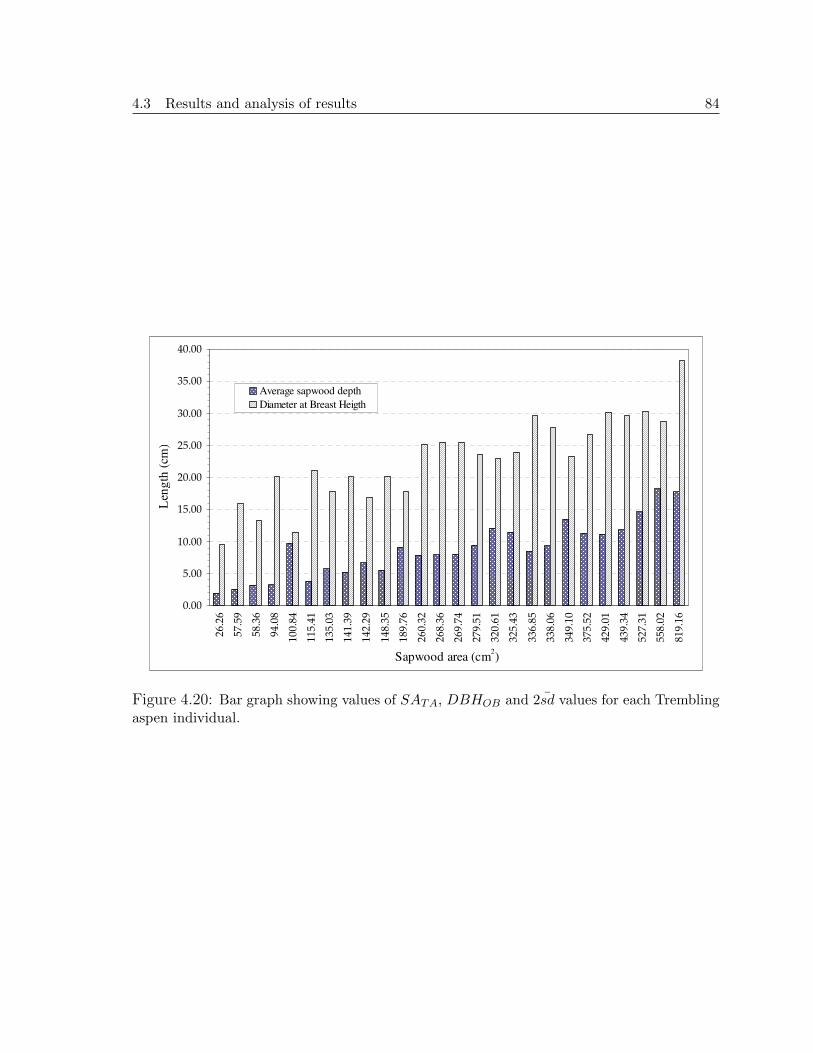
Figure 4.20 shows the corresponding values of 2sd and DBHOB for each tree’s es-
timated SATA. In the whole sample set, there is a large variability in both 2sd and
DBHOB as SATA increases. The clearest trend is for the last six individuals, where 2sd
increases together with size (DBHOB) and SATA. From this figure, it can be appreci-
ated that sapwood area depends on both individual’s DBHOB and 2sd. Small individ-
uals can reach large SATA if 2sd is large (e.g. individual whose SATA is 558.02cm2),
and vice versa, larger trees have a small SATA if 2sd is small (e.g. individual whose
SATA is 148.35cm2).
4.3 Results and analysis of results 84
Sapwood area (cm2)
Len
gth
(cm
)
Average sapwood depth
Diameter at Breast Heigth
Figure 4.20: Bar graph showing values of SATA, DBHOB and 2sd values for each Tremblingaspen individual.
4.3 Results and analysis of results 85
Black spruce. Twenty two Black spruce trees (88 cores) out of 33 were suitable for
analysis with the microscope. This coniferous species presented several problems due
to wood decay and malformations that made the differentiation of sapwood-heartwood
boundaries difficult. As a consequence, 11 trees were dismissed from the sample set, and
6 of them were the ones collected in Whitecourt. Finally, the new Black spruce sample
set remains with 22 individuals, with DBHOB ranging from 9.5cm to 37.9cm. In this
sample set, an outlier was found on the West side of an individual with a DBHOB of
15.28cm (sdcp = 7.30cm). Statistics of sapwood depths for the Black spruce sample set
are given in Table 4.13.
Table 4.13: Basic statistics of the sdcp values obtained from the Black spruce sample set.Individual’s DBHOB ranges from 9.55cm to 37.88cm.
Sapwood depth
Cardinalpoint
Maximum Minimum Mean Mode Variance
(cm) (cm) (cm) (cm) (cm2)
North 5.00 1.60 3.20 2.72 0.92
South 5.10 0.90 3.12 0.90 1.98
East 6.00 0.60 3.64 3.30 2.49
West 5.80 0.90 3.36 0.90 1.82
Maximum sdcp values range between 5.00cm and 6.00cm that pertain to trees whose
9.55cm < DBHOB ≤ 24.51cm. Minimum sdcp values range between 0.60cm and 1.60cm
that pertain to trees whose 9.55cm ≤ DBHOB ≤ 27.06cm. Thus, it seems that sdcp
indistinctly grows around the tree trunk; or at least, with this sample set there is no
evidence to correlate thicker/thinner sdcp to larger/smaller trees.
The last column of Table 4.13 shows each cardinal point’s sapwood depth variance;
this is also appreciated in Figure 4.21. The smallest variance is registered for the sdN
values, followed by the sdW values. On the other hand, sdS values register a slightly
larger variance than sdW values; however, the largest variance is registered for the sdE
values. Note that these sdcp values have similar patterns to the Lodgepole pine and
Jack pine individuals.
4.3 Results and analysis of results 86
Figure 4.21: Dot plot of sdcp values (cm) for the Black spruce sample set. Notice the widespread of the data mostly for the West and East sides.
Each individuals’s sdcp value is plotted against its DBHOB and is shown in Figure
4.22. The variance in each individual’s sdcp values does not show a clear pattern with
respect to its DBHOB. However, ANOVA results concluded that there is still a sig-
nificant difference between the mean values of sdcp and DBHOB (Table 4.14). In this
particular case, the regression analysis will conclusively demonstrate the correlation
between the Black spruce average sdcp and DBHOB (Chapter 5).
Table 4.14: One-way ANOVA between Black spruce sdcp and DBHOB. The null hypothesis(Ho) tests the equality between the sdcp and DBHOB means, where sdcp is the response value(α = 0.05).
Source ofvariation
Degrees ofFreedom
Sum ofsquares
Meansquare
F0 P-value
DBHOB 18 75.69 4.20 4.01 <0.001
Residual Error 61 63.90 1.05
Total 79 139.59
Despite previous results, each Black spruce individual shows a pattern of variation in
sdcp around a tree (as it was for the Jack pine and Lodgepole pine sdcp values). Sixty
seven percent of the Black spruce sample set has the largest sapwood depth at the North
4.3 Results and analysis of results 87
and East sides (38% from the East side and 29% from the North side), while 52% has
the shortest sapwood depth at the South and West sides (38% from the South and 14%
from the West). Furthermore, there are individuals having the largest sapwood depth
at the South-West sides (33% [4% from the South and 29% from the West]) and the
shortest at the North and East sides as well (48% [24% from the East and 24% from
the North]). Thus, results show now that North-East side dominates in the largest
sapwood depth values, and the South-West side develops the smallest sdcp . A one-way
ANOVA with repeated measurements shows that indeed there is not a significant effect
from cardinal direction on sdcp values (Table 4.15).
Table 4.15: One-way ANOVA Black spruce sdcp as a response of cardinal direction (i.e.repeated measurements, α = 0.05).
Source ofvariation
Degrees ofFreedom
Sum ofsquares
Meansquare
F0 P-value
Cardinal direction 3 3.87 1.29 0.906 0.444
Residual Error 60 85.51 1.43
Total 63 89.38
The variance of sdcp variances was calculated for the 21 Black spruce individuals
by grouping them into DBHOB classes. Each diameter class encompasses two 2-inch
classes (i.e. instead of 2-inch classes [as normally is used in forestry], they are 4-inch
classes) to have almost the same quantity of trees per class. The highest sdcp variance
was for trees of 4-inch class, while the lowest variance of sdcp was recorded for trees
larger than 12 inches (Table 4.16). These results point to the fact that the larger the
tree, the lower each individual’s sdcp variance (i.e. each individual’s variance between
sdN , sdS, sdE and sdW ).
Each Black spruce individual’s 2sd was estimated by applying Equation (4.4). Figure
4.23 shows a negative skewed distribution on the Black spruce 2sd values. Two large
accumulations of 2sd values occur in the 7.5cm and 10.0cm classes. The former class
accumulates 38% with a variance between 2sd values of 0.5cm2. Moreover, the 7.5cm
4.3 Results and analysis of results 88
DBHOB (cm)
Sap
wo
od
dep
th(c
m)
North South East West
Figure 4.22: Sapwood depth per cardinal point (sdcp) per each Black spruce tree, versus itsDBHOB. Notice that two values are missing: one sdE and two sdW . Two values were notestimated due to wood decay and one sdW was an outlier (CBHOB = 15.28cm).
Table 4.16: Variance of Black spruce trees sdcp variances (cm4) with re-spect DBHOB. To keep consistency with the forest survey classification,here the DBHOB classes are reported in inches.
Diameterclass
Variance ofvariances
(inches) (depth)
4-7 3.82
8-11 1.27
12-15 0.42
2sd class is integrated by trees with a DBHOB ranging between 11.1cm to 37.9cm
(s2 = 60.34cm2). Similarly, the latter class of 2sd values is about 38% with an s2 =
0.5cm2; and DBHOB’s ranging between 15.3cm and 35.3cm (s2 = 47.8cm2). Nineteen
percent of the Black spruce individuals are in the 5cm 2sd class, with DBHOB values
4.3 Results and analysis of results 89
that varied from 9.5cm to 29.9cm (s2 = 101.9cm2). The remaining 5% pertains to the
2.5cm 2sd class and includes one individual of 25cm in DBHOB. From these results, it
is observed that there is a large variance of DBHOB values in each 2sd class. In fact,
individuals with a DBHOB of ≈ 24cm can be found in the 7.5cm or the 10.0cm 2sd
classes. Even individuals with a DBHOB of ≈ 26cm can be found in the 5cm, the 7.5cm
or the 9.5cm classes. Thus, 2sd seems to be independent of the individual’s DBHOB.
Average sapwood depth classes (cm)
Cla
ssfr
equ
ency
(%)
Figure 4.23: Black spruce sample set histogram of 2sd values.
The Black spruce sapwood area (SABS) histogram shows a positive skewed distribu-
tion (Figure 4.24). The most common SABS values fall into the class of 250cm2 and
holds 38% of the sampled trees, whose DBHOB range from 19.4cm to 29.9cm. Next
common SABS values are in the 150cm2 class (29% of the total sample set) correspond-
ing to trees between 9.5cm and 27.1cm in DBHOB. The last two SABS classes hold the
remaining 33% of the sample set, and also the largest trees (DBHOB between 23.9cm
and 37.9cm).
4.3 Results and analysis of results 90
Sapwood area (cm2) classes
Cla
ssfr
equ
ency
(%)
Figure 4.24: Black spruce sample set histogram of SABS values.
Figure 4.25 shows the corresponding 2sd and SABS values for each Black spruce
individual according to its DBHOB. As it did occur with the other coniferous species,
there are particular cases in which a large SABS is registered for relatively small trees
that have large sapwood depth. Indeed, individuals with very small 2sd but large
DBHOB, register large SABS values. Specifically, a tree as large as 27.1cm in DBHOB
having a small 2sd (2.15cm) will of course have its SABS equal to 87.7cm2. Also, look
at the tree with an SABS of 375.59cm2, whose DBHOB is one of the largest, but its
2sd is even smaller than a tree with one of the smallest DBHOB. Thus, the increments
in SABS do not correspond to sapwood depth increments, but the tree size.
4.3 Results and analysis of results 91
Sapwood area (cm2)
Len
gth
(cm
)
Average sapwood depth
Diameter at Breast Height
Figure 4.25: Bar graph showing values of SABS , DBHOB and 2sd values registered for eachBlack spruce individual.
4.3 Results and analysis of results 92
White spruce. It was possible to analyse under the microscope the whole White spruce
sample set (68 wood cores). Thus, the sample set size did not change and remains with
18 individuals, whose CBHOB range from 11.5cm to 50cm. Statistics of measured
sapwood depths in the four cardinal points are given in Table 4.17.
Table 4.17: Basic statistics of the sdcp values obtained from the White spruce sample set.Individual’s CBHOB ranges from 11.5cm to 50cm.
Sapwood depth
Cardinalpoint
Maximum Minimum Mean Mode Variance
(cm) (cm) (cm) (cm) (cm2)
North 5.20 1.50 3.22 4.40 1.17
South 5.60 1.72 3.37 2.30 1.50
East 4.90 0.69 2.87 3.10 1.64
West 5.90 0.35 3.19 4.20 2.33
Maximum sdcp values range between 4.90cm and 5.90cm that were measured in trees
whose DBHOB > 28.18cm (i.e. the average DBHOB). Minimum sdcp values range
between 0.35cm and 1.72cm that pertain to trees whose DBHOB ≤ 28.18cm. Here,
there is not a window for considering any correlation between the thickness of sapwood
depth and the tree size, because three of the minimum values pertain to a tree whose
DBHOB = 11.46cm. With respect to the maximum sdcp values, all of them pertain to
different trees, and as mentioned before, they are larger than the mean DBHOB of the
White spruce sample set.
In Figure 4.26 and the last column of Table 4.17, it is shown that the largest variance
is for sdW values, with lower variations for sdE and sdS. The smallest variance was
observed for the sdN values; nevertheless, it is still a large variance (1.17cm2) taking
into account the registered lengths in sapwood depth.
As a result, there is a change of sdcp values as the individual’s DBHOB changes.
This change is observed in Figure 4.27, where each individuals’s sdcp values is plotted
against its DBHOB. Similar to Trembling aspen, each individual’s sdcp generally tend
to increase as their DBHOB increases. The ANOVA testing the similarity between mean
4.3 Results and analysis of results 93
Figure 4.26: Dot plot of sdcp values (cm) for the White spruce sample set. In general, thereis a wide spread of sdcp in every cardinal point, being the largest at the East and West sides(Same as it occurs for the other three coniferous species).
values of sdcp and DBHOB drew similar conclusions: there is a significant difference
between mean values (Table 4.18). Therefore, it can be concluded that changes in
sdcp are driven by changes in DBHOB (assuming that the cardinal direction has no
significant effect on sdcp ). Still, more information will be derived after the regression
analysis between these two variables.
Table 4.18: One-way ANOVA between White spruce sdcp and DBHOB. The null hypothesis(Ho) tests the equality between the sdcp and DBHOB means, where sdcp is the response value(α = 0.05).
Source ofvariation
Degrees ofFreedom
Sum ofsquares
Meansquare
F0 P-value
DBHOB 16 68.968 4.311 7.01 <0.001
Residual Error 49 30.137 0.615
Total 65 99.105
As it occurs with the rest of the species studied here, each White spruce individual
registers a maximum, minimum and intermediate sdcp value. On the other hand, each
individual’s sdcp variance remains fairly small, and it tends to increase in the bigger trees
4.3 Results and analysis of results 94
(DBHOB ≥ 31.8cm). Fifty nine percent of the sample set has the largest sapwood depth
at the South and West sides, while 53% of the sample set has the smallest sapwood
depth at the North and East sides. Furthermore, the smallest sdcp values were also
observed at the South and West sides (47%), and 41% of the sample set registers the
largest sdcp values at the North and East sides. The maximum and minimum sdcp values
seem to be quasi evenly distributed around the tree trunk. A one-way ANOVA with
repeated measurements shows that indeed there is no significant effect from cardinal
direction on sdcp . Thus, it seems that there is no preference in White spruce to grow
thicker or thinner in a specific direction (Table 4.19). Be aware that the last conclusion
is totally independent of the fact that each White spruce individual still has a maximum,
minimum and intermediate sdcp around the tree trunk.
Table 4.19: One-way ANOVA White spruce sdcp as a response of cardinal direction (i.e.repeated measurements, α = 0.05).
Source ofvariation
Degrees ofFreedom
Sum ofsquares
Meansquare
F0 P-value
Cardinal direction 3 6.31 2.10 2.41 0.078
Residual Error 51 44.51 0.87
Total 54 50.82
The variance of sdcp variances is shown in Table 4.20. The highest sdcp variance
was for trees of the 8-inch class, while the lowest variance was recorded for trees in
the 6-inch class. Unlike the other species, White spruce has a larger variance in sdcp
values for larger individuals. For middle size individuals (6-inch class), the variance in
between sdcp values was minimal.
With respect to the calculated 2sd, the sample set values have a distribution close
to Normal (Figure 4.28). The largest accumulation of 2sd values is for the two middle
classes (i.e. 5.5cm and 8.0cm). Specifically, 41% of the 2sd values fall between 5.6cm
and 8.0cm with a variance between 2sd values of 0.45cm2. Into this 8cm 2sd class,
DBHOB values varied from 25.5cm to 35.6cm (s2 = 14.6cm2). The 5.5cm 2sd class
4.3 Results and analysis of results 95
DBHOB (cm)
Sap
wo
od
dep
th(c
m)
North South
East West
Figure 4.27: Sapwood depth per cardinal point (sdcp) per each White spruce tree, versus itsDBHOB. There are two missed sdE values. One sdE is missed since it was not possible tosample the individual in that side. The second sdE value was dismissed due to wood decay.
Table 4.20: Variance of White spruce trees sdcp variances(cm4)with respect DBHOB. To keep consistency with theforest survey classification, here the DBHOB classes are re-ported in inches.
Diameterclass
Variance ofvariances
(inches) (depth)
4-5 0.20
6-7 0.03
8-9 0.78
holds 35% of the total sample set and its variance between sd values equals 0.40cm2;
DBHOB values in this class range from 14.0cm to 23.5cm. Eighteen percent of the
sample set integrates the 10.5cm class, whose individuals’ DBHOB range from 38.5cm
to 50.0cm. The remaining 6% is a tree with a 2sd of 2.66cm and DBHOB of 11.5cm,
which is the smallest tree of the sample set. For two individuals, their sdE value was
4.3 Results and analysis of results 96
dismissed due to wood decay; thus, their 2sd was estimated as an average of the sdN ,
sdS and sdW values.
Average sapwood depth classes (cm)
Cla
ssfr
equ
ency
(%)
Figure 4.28: White spruce sample set histogram of 2sd values.
The White spruce sapwood area (SAWS) histogram is in Figure 4.29. The histogram
shows two large accumulations of SAWS values, the first and largest one pertains to the
101 − 200cm2 class (with 29% of the SAWS values), and the next one pertains to the
301− 400cm2 class (with 23.5% of the SAWS values). The SAWS class of 101− 200cm2
includes trees with a DBHOB of 15.9cm to 23.5cm, while the 301−400cm2 class includes
trees with a DBHOB between 38.8cm and 35.7cm.
Following these two classes, there are four more SAWS classes that hold the rest of
the sample set. First, 18% of the sample set falls into the 201−300cm2 class, including
those trees whose DBHOB values range between 25.5cm and 28.3cm. Second, 12% of
the White spruce trees fall into the 42 − 100cm2 SAWS class, corresponding to the
smallest trees of the sample set (DBHOB ranges between 11.5cm and 14cm). Next
class includes trees whose SAWS falls between 601cm2 and 700cm2 and whose DBHOB
are the largest of the sample set (46.8cm and 50cm). Finally, one tree (≈ 6% of the
4.3 Results and analysis of results 97
0.00
5.00
10.00
15.00
20.00
25.00
30.00
35.00
Sapwood area (cm2) classes
Cla
ssfr
equ
ency
(%)
Figure 4.29: White spruce sample set histogram of SAWS values.
0.00
5.00
10.00
15.00
20.00
25.00
30.00
35.00
40.00
45.00
50.00
55.00
42
.25
83
.84
10
0.1
5
11
2.8
8
12
0.0
7
12
3.9
5
16
9.7
2
23
1.2
7
24
3.9
7
29
2.2
3
33
4.3
9
34
5.9
8
38
2.4
4
38
3.3
5
44
3.2
9
64
2.8
8
66
5.1
1
Sapwood area (cm2)
Len
gth
(cm
)
Average sapwood depth
Diameter at Breast Height
Figure 4.30: Bar graph showing values of SAWS , DBHOB and 2sd values register for eachWhite spruce individual.
4.3 Results and analysis of results 98
sample set) with a DBHOB of 38.5cm fall into the 400 − 500cm2 SAWS class.
In the particular case of the White spruce, each SAWS class corresponds to only
one range of DBHOB values. That is, the DBHOB ranges do not overlap with one
another, and as the DBHOB increases, the SAWS increases as well. This relationship is
also observed in Figure 4.30 where 2sd values are also included. In general, the graph
shows that increments in SAWS correspond to increments in DBHOB, while 2sd values
remain fairly constant along the DBHOB range. Thus, unlike the other three coniferous
species, increments in SAWS are driven by tree size, and there are changes in 2sd as
the tree grows.
4.3.4 Comparison between methods to measure sapwood depth
Microscopical analysis and translucence methods. The sample sets of White spruce,
Jack pine, and Lodgepole pine were used for measuring sapwood depth by the translu-
cence and microscopical analysis.
For the White spruce sample set, a Paired-T test proved that the two set of results are
significantly different (P=0.00, N=36) with α = 0.05. Similarly, in the Jack pine and
Lodgepole pine sample set, the obtained sapwood depth values with the two different
methods are significantly different (P=0.00, N=50) with α = 0.05. It is concluded
that the two methods for measuring sapwood depth will give different estimates for
individuals of White spruce, Jack pine and Lodgepole pine individuals.
In White spruce, the difference between the sapwood depth measured by the translu-
cence method and microscopical analysis (sdtranslucence - sdmicroscopic [i.e. the paired
response differences]) ranged between −1.10cm and 1.60cm. Figure 4.31 is the plot
of the paired response differences that clearly shows a constant overestimation of the
sapwood depth by the translucence method. More importantly is how the method used
to estimate sapwood depth affects the estimation of total sapwood area. The estimated
White spruce sapwood areas by means of the sd values obtained with the two methods
showed a significant difference that ranged between −18.02cm2 and 71.92cm2 (Figure
4.32). In 77% of the cases, White spruce’s sapwood area was overestimated by the
4.3 Results and analysis of results 99
translucence method. The maximum overestimation was of 34% of the total sapwood
area estimated with the microscopical method. On average, the overestimations were
approximately 15% of the total sapwood area estimated with the microscopical method.
Figure 4.31: Plot of the paired response differences between sdcp values obtained with themicroscopical analysis and the translucence methods. White spruce sample set. Notice thatfive values are missing because they overlap.
In the Jack pine and Lodgepole pine sample set, the difference between the sapwood
depth measured by microscopical analysis and the translucence method ranged between
−4.90cm and 1.90cm. The plot of the response differences (Figure 4.33) shows that it
was more common to have an underestimation of the sapwood depth by the translucence
method. The estimated Jack pine and Lodgepole pine sapwood areas by means of
the sd values obtained with the two methods showed residuals that ranged between
−102.06cm2 and 37.86cm2 (s = 36.52cm2). There is a constant underestimation (86%
of the cases) of the sapwood area by the translucence method (Figure 4.34) with an
average of 35% of the total sapwood area estimated with the microscopical method.
The largest underestimation was of 61% of the total sapwood area calculated with the
microscopic method.
4.3 Results and analysis of results 100
Figure 4.32: Plot of the paired response differences between measured sapwood area withthe microscopical analysis and the translucence methods. White spruce sample set.
In terms of the uncertainty associated with the translucence method, it is difficult to
estimate it because it is a function of the gross and systematic errors. Both types of
error are difficult to measure because they are related to the person who determines the
translucent sapwood depth. The only guidance for the translucence method is that the
sapwood transmits light while the heartwood does not. This criterion does not have a
solid basis (as explained in § 4.1.1) since the wood water content varies and confounds
both sapwood and heartwood. On the contrary, the uncertainty associated with the
wood tissues microscopical analysis method can be estimated, and taken into account
for further estimations or predictions.
Microscopical analysis and Coloration methods. The coloration method was tested
with the Trembling aspen sample set. For a total of seventeen wood cores, sapwood
depth values were obtained with both the microscopical analysis and the coloration
methods. The number of tested wood cores was limited by how problematic it was to
4.3 Results and analysis of results 101
Figure 4.33: Plot of the paired response differences between sd values obtained with themicroscopical analysis and the translucence methods. Jack pine and Lodgepole pine sampleset.
distinguish the difference in coloration between the sapwood and heartwood. Still, the
sample size is adequate for performing a Paired t-test (α/2 = 0.1 and β = 0.8). Thus,
the obtained sapwood depth values with the two different methods are significantly dif-
ferent (P=0.012, α/2 = 0.1). It can be concluded that the two methods for measuring
sapwood depth will give different estimates when it comes to Trembling aspen individu-
als. For sapwood depth values, the paired difference between the microscopical analysis
and the coloration methods ranged from 0.00cm to −1.8cm (Figure 4.35). In 65% of the
cases, Trembling aspen’s sapwood depth was underestimated by the coloration method;
in the remaining 35% of the cases the measured sapwood depth was exactly the same
for both methods (i.e. the paired difference was null). In terms of sapwood area, the
largest underestimation was approximately 18% of the total area calculated with the
microscopical analysis method. On average, the underestimations were 10% of the total
area calculated with the microscopical analysis method.
In summary, the translucence and coloration methods are already considered unreli-
4.3 Results and analysis of results 102
Figure 4.34: Plot of the paired response differences between sapwood area values obtainedwith the microscopical analysis and the translucence methods. Jack pine and Lodgepole pinesample set.
able (Cermak and Nadezhdina, 1998). Here, the obtained results quantify the reliability
of the methods, which is closely related the physiological criteria for distinguishing sap-
wood from heartwood. Thus, the two methods over and underestimated sapwood depth.
The overestimation was notorious in White spruce individuals, while underestimations
commonly occurred in Trembling aspen and Jack/Lodgepole pine individuals. The re-
ported percentages quantify the over and underestimations and they could be used as
a way of estimating the translucence and coloration methods’ uncertainty.
4.3 Results and analysis of results 103
Figure 4.35: Measured sapwood depth paired difference between the microscopical analysisand the coloration methods. Trembling aspen wood cores of different DBHOB.
4.4 Discussion and Conclusions 104
4.4 Discussion and Conclusions
To evaluate the preciseness of sapwood depth as scaling factor, it was necessary to
analyze within-tree variation, and the sapwood depth variability with respect to the
species and tree size. And at the same time, it was important to recognize the influence
of the bio-physical factors in tree growth. Thus, the following discussion is based on
the obtained results and previous knowledge of the bio-physical conditions under which
the five studied species grow.
Each studied species’ sdcp results concur with previous works stating that the depth
in sapwood is not homogenous around the tree annulus along the tree trunk (Kozlowski
and Pallardy, 1997; Philipson et al., 1971b,a). Thus, sapwood depth heterogeneity at
the four cardinal points suggests that it is necessary to measure sapwood depth at least
in the four cardinal points for obtaining a reliable sapwood depth estimate.
Also, the five studied species tend to have a small sdS values which, is attributed to
the fact that in the Northern Hemisphere, the South sides are exposed to much more
solar radiation than North-facing slopes (Auslander et al., 2003); thus, the South sides
tend to have xeric conditions that are a constraint for the trees with respect to water
availability and variability in microclimate. Hence, it is believed that trees tend to have
less sdS as a mechanism of defence (i.e. to avoid loosing large amounts of water).
In comparison with the other three coniferous species, the Black spruce sdcp and sd
values have the lowest variance which could be attributed to tree growth requirements.
This species is prone to grow under high soil moisture conditions. Thus, Black spruce
individuals are normally found in flat areas, where there are high water concentrations
and the sunlight will be more evenly distributed at the four cardinal points along the
day than on terrains with slope. As a consequence, sapwood in Black spruce has similar
chances to grow at any side of the tree.
In Jack pine and Lodgepole pine individuals there is low variance in sdW and sdN
that may be attributed to a well balanced supply of water (mesic conditions) in the
North-facing sides (remember that most of the samples were collected in sites with a
4.4 Discussion and Conclusions 105
North-East aspect). Moreover, in Lodgepole pine and Jack pine individuals there is a
small variance of 2sd as the individuals grow. It may imply that for these two species
in particular, the tree sapwood depth does not largely vary as the individuals grow.
Unlike these two species, White spruce and Trembling aspen species 2sd increases at
larger DBHOB. Thus, in the case of White spruce and Trembling aspen it is concluded
that indeed, sapwood depth is directly proportional to DBHOB. Consequently, SAWS
and SATA estimates show proportional increments with respect to DBHOB and 2sd.
In contrast, increments on SAJP , SALP , and SABS estimates are mainly related to
increments in DBHOB and not to 2sd. As mentioned, some of the largest trees in
DBHOB registered small 2sd values, but still they have large SAsp due to the influence
of their CBHOB.
All crown classes of sampled trees were relatively high. It has been suggested that
crown class my be another factor influencing sapwood depth. For instance, one White
spruce tree of 44cm in DBHOB showed a 2sd similar to that of a small tree of 22cm
in DBHOB due to its very low crown class. Thus, it may be suggested to integrate
crown class as another factor influencing sapwood depth; however, crown class is not
rigorously defined. Thus, if the crown class classification is a subjective method, it
could be a hindrance in obtaining objective outcomes.
In conclusion, sapwood depth and sapwood area seem to behave differently in each
studied species and are not always proportional to the tree size as it is normally assumed.
It appears that the structural design and growth of sapwood depth and sapwood area
is species-specific and one should be cautious in assuming similar tree growth patterns
in non-studied tree species. Thus, in order to effectively use either sapwood depth
or sapwood area as scaling factors, it is recommended that one observe each species
sapwood depth variations before making any inference. Also, it is important to specify
the environmental conditions and species growth requirements as factors that might
influence the allometric correlations of sapwood depth. These results help to better
understand of how sapwood varies along a tree trunk and between different tree sizes,
which will allow one to obtain more reliable predictions of sapwood depth and sapwood
area.
4.4 Discussion and Conclusions 106
4.4.1 Future work
Similar studies are needed in order to reinforce previous results and to observe the
variations of sapwood depth and sapwood area in different site conditions, such as
slope, aspect, and climate. Also, studies rigorously classifying trees by crown class will
give an insight of sapwood depth variations in relation to the trees spatial location, and
its influence on plot transpiration rates.
5 Allometric correlations
Chapter outline
The calculation of a tree transpiration rate by means of sap flow density uses the
sapwood area as the scaling factor (Granier, 1985). Measuring sap flow density and
sapwood area at each studied tree becomes a complex and destructive method when
estimating a whole tree stand’s transpiration. As a consequence, it would be convenient
to adopt an alternative method for aggregating transpiration rates at the stand (i.e.
plot) scale.
For this research it is crucial to obtain a scaling parameter to aggregate tree tran-
spiration rates to the plot scale. For that, it is necessary to develop an allometric
relationship between two measurable vegetation factors per plot. Based on Shinozaki’s
pipe model theory that a proportion of sapwood cross-sectional area transports water
and nutrients to a specific amount of leaf area (Smith and Hinckley, 1995), it is ex-
pected that this relationship holds true at the plot scale. Furthermore, it is supposed
that sapwood area and leaf area are the adequate scaling parameters due to their close
relationship with transpiration.
Thus, the expected aims of this research dissertation chapter are:
1. Develop sd :DBHOB allometric correlations for the five species of interest.
2. Develop an approach to aggregate a single tree’s sapwood area to the plot’s scale
(i.e. plot’s sapwood area).
3. Develop plot sapwood area : leaf area correlations taking into account the plot’s
vegetation heterogeneity.
107
5.1 Modelling SAplot :LAplotSAplot :LAplotSAplot :LAplot relationship 108
To the author’s knowledge, there is no published work developing a plot’s sapwood
area - leaf area relationship (SAplot : LAplot). The published work in this matter deals
with single tree relationships (e.g. Gilmore et al. (1996); Kaufmann and Troendle
(1981); McDowell et al. (2002); Meadows and Hodges (2002)). These works have re-
ported different sapwood area : leaf area correlations for the same species, attributing
the discrepancy to site-specific characteristics, stand density, and tree competition.
The concept used to estimate a plot’s sapwood area and leaf area defines a vegetated
plot as a surface area that holds a big, single tree, whose vascular and leafy parts will
be the summation of all the tree’s vascular and leafy parts inside the plot. For instance,
the big tree’s sapwood area could become an integration of each species sapwood area
present in the plot.
This chapter then presents the results of single tree sapwood area models, the aggre-
gation of sapwood area to the plot scale, and plot sapwood area models. At the tree
scale, sapwood area was estimated by previously defining the sd : DBHOB relationship.
At the plot scale, Leaf Area is the parameter used as the predictor of Sapwood Area.
The obtained linear regression models were tested and statistically analysed.
5.1 Modelling SAplot :LAplotSAplot :LAplotSAplot :LAplot relationship
5.1.1 Introduction
Sapwood area supports several physiological functions, such as photosynthesis, gas ex-
change, cooling, nutrient transport, and naturally transpiration. Also, sapwood area
has been theoretically related to leaf area (Shinozaki’s pipe model theory, Smith and
Hinckley, 1995). The pipe model theory has been sufficiently proven by several re-
searchers’ work. Most of these works have modeled the leaf area : sapwood relationship
area (LAsp :SAsp) to estimate a single tree’s leaf area having sapwood area as the pre-
dictor. These works have reported linear models for about 20 conifers, such as Scotch
pine ([Pinus sylvestris ], Whitehead, 1978), Ponderosa pine ([ Pinus ponderosa], War-
5.1 Modelling SAplot :LAplotSAplot :LAplotSAplot :LAplot relationship 109
ing, 1982), Loblolly pine ([Pinus taeda], Blanche et al., 1985), Douglas fir ([Pseudotsuga
menziesii ], Borghetti et al., 1986; Waring, 1982; McDowell et al., 2002), Lodgepole pine
([Pinus contorta, Dean et al., 1988; Hungerford, 1987; Keane and Weetman, 1987; Kauf-
mann and Troendle, 1981), Engelmann spruce and Subalpine fir ([Picea engelmanni and
Abies lasiocarpa], Kaufmann and Troendle, 1981), Pinyon pine and One-seeded Juniper
([Pinus edulis and Juniperus monosperma, Schuler and Smith, 1988), Balsam fir ([Abies
balsamea], Coyea and Margolis, 1992; Marchand, 1984), and so forth.
Deciduous species haven’t been as studied as coniferous species; however, still there is
some published work by Vertessy et al. (1995) for Mountain ash (Eucalyptus regnans),
Kaufmann and Troendle (1981) for Trembling aspen (Populus tremuloides), Meadows
and Hodges (2002) for Cherry bark oak (Quercus falcata) and Green ash (Fraxinus
pensylvanica). In this last work, Meadows and Hodges (2002) improved their model
for predicting leaf area by not only having sapwood area as a predictor, but by adding
total height and live crown ratio to the equation.
Researchers that have studied the same species under different site conditions, have
reported different LAsp : SAsp linear (even sometimes non-linear) equations. The dis-
crepancy between results have helped to understand that the LAsp :SAsp relationship is
driven by the site’s conditions such as stand density (Binkley and Reid, 1984; Shelburne
et al., 1993; White et al., 1998), climatic factors (Mencuccini and Grace, 1994), and
physical characteristics (Hillis, 1987). Naturally, it is expected that the LAsp :SAsp re-
lationship is species-specific (Hillis, 1987), but it does not always happen. For instance,
Dean and Long (1986) determined that the Lodgepole pine’s allometric relationship
LAsp : SAsp is linear, while Kaufmann and Troendle (1981) determined that a non-
linear regression better explains the relationship. Thus, while in theory the correlation
LAsp :SAsp is explained as linear, it could change due to site conditions.
In the present study, it is suggested that besides the site conditions, the methods
used to measure sapwood area and leaf area significantly influence the LAsp : SAsp
relationship. It is well known that not all the methods to measure sapwood area will
give the same results (Cermak and Nadezhdina, 1998), and direct or indirect leaf area
5.1 Modelling SAplot :LAplotSAplot :LAplotSAplot :LAplot relationship 110
mensuration gives different outcomes as well (Jonckheere et al., 2004).
In more recent work, the average sapwood thickness (i.e. average sapwood depth, sd)
has been used instead of sapwood area to indirectly estimate some other forest stand
characteristics such as canopy cover densities and foliage biomass by combining remotely
sensed data and field data (Lefsky et al., 1999; Means et al., 1999). The method consists
of estimating foliage biomass as a function of DBH by previously modelling sd :DBH
relationships to predict DBH for a whole tree stand (Means et al., 1999). The authors
used previous equations to estimate foliage biomass and sapwood area. In a similar way,
Lefsky et al. (1999) used an already published sd :DBH relationship to estimate foliage
biomass as an indicator of DBH. The sd :DBH relationship used by both authors was
obtained from Lassen and Okkonen (1969).
To the author’s knowledge, Lassen and Okkonen (1969) could be one of the few
published works reporting results for single tree sd : DHB relationships (Lassen and
Okkonen’s paper cited 3 more published works on this issue). Lassen and Okkonen
reported that in Douglas-fir (Pseudotsuga menziesii) and some other conifers, sapwood
depth increases as the tree’s diameter (inside bark) increases. Most of the species showed
that trees had an exponential sapwood depth growth until they reached a diameter
of 25.4 − 38.1cm; thereafter, sapwood depth nearly reached a plateau. Thus, trees’
sapwood depth tend to increase “only slightly” in older/bigger trees. That was the
general tendency, with the exception of Lodgepole pine that showed a large variability
in sapwood depth, and actually some trees that were smaller in diameter showed a
larger sapwood depth than those with a larger diameter. Authors also concluded that
Douglas-fir trees with the same diameter had different sapwood depths according to
their location (coast area or interior land), and elevation.
Even though there is sufficient work supporting the strong relationship between a
single tree’s sapwood area and leaf area, these models cannot be used to scale up to
larger scales. In a forested region, it is expected that leaf area increases as the ground
area increases, it is not possible to use single tree models to interpolate either leaf area
or sapwood area values for a group of trees. Thus, it is necessary to develop specific
5.1 Modelling SAplot :LAplotSAplot :LAplotSAplot :LAplot relationship 111
models for the SAplot :LAplot relationship.
5.1.2 Material and methods
Statistical Analysis. All the statistical analyses were mainly performed with Minitab,
version 13.32 (Minitab Inc., State College, PA USA). For each species, there was an
exhaustive study of the statistical results to determine the most adequate model. These
statistical results include the Pearson’s correlation coefficient, detection of outliers,
the regression analysis, the ANOVA, list of unusual observations, and the lack-of-fit
test. Finally, each linear model’s residuals were examined in order to check the model
adequacy. Model adequacy checking includes a Normal plot of residuals and the plot
of residual versus fitted values.
Besides the correlation analysis, the pairwise comparison of the Coefficient of Vari-
ation (COV ) confidence intervals (C.I.) is used as an indication of the relationship
between the scaling parameters at the plot scale (i.e. between Sapwood Area [SAplot]
and Leaf Area Index, and between SAplot and Leaf Area [LAplot]). The pairwise com-
parison consists of comparing the parameters’ C.I. to see if they overlap or not. This is
another way to test if there is correlation between the variables; since they are different
parameters and the units differ, it is not suitable to use mean values or standard devi-
ations to test the similarity between the two sample populations (Payton et al., 2000;
Vangel, 1996; Verrill, 2003).
Thus, for 100 (1 − α)% and ν = n − 1 degrees of freedom, the modified McKay
Confidence Interval for a COV (Vangel, 1996) is:
[(
u1 + 2
n− 1
)
K2 +u1
ν
]
−0.5
K ≤ COV ≤ K
[(
u2 + 2
n− 1
)
K2 +u2
ν
]
−0.5
(5.1)
where K is the point estimate of COV (K = S/X), u1 = χ2ν,1−α/2, and u2 = χ2
ν,α/2.
Therefore, K is a function of the sample standard deviation (S), and the sample mean
(X).
5.1 Modelling SAplot :LAplotSAplot :LAplotSAplot :LAplot relationship 112
Another modified approach to MacKay C.I. is suggested by Payton (1997):
χ2ν,1−α/2
[
1 + K2
nK2
]
−0.5
≤ COV ≤ χ2ν,α/2
[
1 + K2
nK2
]
−0.5
(5.2)
The main difference between both Equations is that the latter one can be used for
any COV value, while Equation (5.1) is restricted to 0 < COV ≤ 0.33 (Vangel, 1996;
Verrill, 2003). C.I. are reported together with the pairwise comparison results.
Development of allometric correlations. To study the SAplot : LAplot relationship,
a vegetated plot has been conceptualized as a surface ground area with a single big
tree whose sapwood area is the summation of all the trees’ sapwood area inside the
plot. Likewise, the big tree’s leaf area will be the summation of all trees’ leaf area
inside the plot. Despite the simplicity of the concept, it takes into account vegetation
heterogeneity.
Based on this concept, allometric correlations and linear models were developed here
in order to measure sapwood area at the tree and at the plot scale. At the tree scale,
the models are firstly based on each species sd and DBHOB data. The obtained cor-
relations were used to estimate each tree’s sapwood area inside the delimited plots and
to aggregate sapwood area at the plot scale.
The plot’s sapwood area estimates were derived by two different approaches. The
first approach was by the previously defined sd :DBHOB correlations per species. The
second approach was by using sapwood area average values, and it was taken as an
alternative when the sd :DBHOB correlation was null. The leaf area per plot, LAplot,
was derived from LAI mensurations and the surface ground area of interest. It was
understood that modelling SAplot : LAplot carries uncertainties while aggregating to
large areas. Thus, uncertainties were estimated through propagation error equations
and reported here in this chapter.
5.1 Modelling SAplot :LAplotSAplot :LAplotSAplot :LAplot relationship 113
Sampling design. Plots of different sizes are used to compare the responses of SAplot :
LAplot. Four plots are of 60×60m, and nine of 10×10m. These plots are located in
the Sibbald Areas of Kananaskis Country, Alberta. The species composition of these
plots was either dominated by deciduous trees (mainly Trembling aspen), or coniferous
trees (Lodgepole pine and White spruce). Figures 5.1 and 5.2 show the location and
delimitation of the plots. Two more plots were delimited at Whitecourt, one dominated
by Jack pine individuals and one dominated by Black spruce individuals. The Jack pine
plot was 20 × 20m, and the Black spruce plot was 15 × 15m. The plots were labelled
as Coniferous for those whose species composition was dominated by a conifer tree,
and Deciduous for those whose species composition was dominated by a deciduous
tree. The site characteristics are considered to be uniform between plots with similar
species composition, with the exception of the Black spruce plot. The Black spruce plot
is located in a lowland area with hydric, organic soil (very poor drainage conditions).
The smallest plots (10×10m) were distinguished from the largest ones (≥ 300m2) by
adding a prime symbol in front of their assigned number.
Field data collected at each plot include number of trees per plot, each tree’s DBHOB,
and Leaf Area Index. Mensurations of LAI were taken in the 60×60m plots using the
Tracing Radiation and Architecture Canopies (TRAC, 3rd Wave Engineering Co.; Ne-
pean, Canada) device. The Canopy Analyzer LAI-2000 (LI-COR Incorporated; Lincoln
Nebraska, US) was used at the two plots located in Whitecourt.
Saplings. It goes without saying that saplings practically lack heartwood, being mostly
composed of sapwood (Kramer and Kozlowski, 1979; Hillis, 1987; Cermak and Nadezh-
dina, 1998). Thus, saplings correlations between DBHOB and sd, or between DBHOB
and SAsp will be different and it is assumed therefore that such correlations have to
be treated separately from the rest of the trees. Saplings are considered to be those
trees whose DBHOB range is ≈ 2.41cm − 10.2cm (or a CBH ≈ 7.6cm − 32.0cm), and
38.1cm − 76.2cm tall. Saplings are not included in any of the allometric correlations.
Thus, all trees found inside of the plots with a DBHOB ≤ 10cm were dismissed. The
studied sites do not hold significant quantities of saplings (see § 5.2 for details).
5.1
Modellin
gS
Aplo
t :LA
plo
tS
Aplo
t :LA
plo
tS
Aplo
t :LA
plo
trelation
ship
114
637900.000000
637900.000000
638100.000000
638100.000000
638300.000000
638300.000000
638500.000000
638500.000000
56
54
60
0.0
00
00
0
56
54
60
0.0
00
00
0
56
54
80
0.0
00
00
0
56
54
80
0.0
00
00
0
56
55
00
0.0
00
00
0
56
55
00
0.0
00
00
0
56
55
20
0.0
00
00
0
56
55
20
0.0
00
00
0
56
55
40
0.0
00
00
0
56
55
40
0.0
00
00
0
0 100 200 30050
Meters
!"#$%
#"
& "'&()
*
Figure 5.1: Geographical location of Coniferous plots. The plots are in the Sibbald areas of Kananaskis Country.Contour lines were extracted from the Base Features GIS (AltaLIS, 2006), 1:20,000. Aspect was retrieved fromthe GEODE archive’s Digital Elevation Models (100m grid, [MADGIC (2006)]).
5.1
Modellin
gS
Aplo
t :LA
plo
tS
Aplo
t :LA
plo
tS
Aplo
t :LA
plo
trelation
ship
115
635500.000000
635500.000000
635700.000000
635700.000000
635900.000000
635900.000000
636100.000000
636100.000000
56
53
60
0.0
00
00
0
56
53
70
0.0
00
00
0
56
53
80
0.0
00
00
0
56
53
90
0.0
00
00
0
56
54
00
0.0
00
00
0
56
54
10
0.0
00
00
0
56
54
20
0.0
00
00
0
56
54
30
0.0
00
00
0
56
54
40
0.0
00
00
0
0 100 20050
Meters
! "!#$
%
&
' (
)
*
Figure 5.2: Geographical location of Deciduous plots. The plots are in the Sibbald areas, South-East of BarrierLake ( Kananaskis Country). Contour lines and Hydrographic features were extracted from the Base FeaturesGIS (AltaLIS, 2006), 1:20,000. Aspect was retrieved from the GEODE archive’s Digital Elevation Models (100mgrid, [MADGIC (2006)]).
5.2 Results and analysis of results 116
5.2 Results and analysis of results
The obtained results are divided in three main parts. The first part describes and
analyses each species sd : DBHOB allometric correlations. The second part is the
description of the theory behind the estimation of sapwood area per species (SAsp) and
plot’s Leaf Area (LAplot). The theory also describes the aggregation of sapwood area
to the plot scale (SAplot) by combining two scaling approaches. The third and last part
describes and analyses the SAplot :LAplot relationship. Finally, the developed equations
for estimating error propagation are described.
5.2.1 Tree scale allometric correlations
Jack pine, Lodgepole pine. The sample sets of Jack pine and Lodgepole pine are
integrated in a single group to obtain sapwood depth and sapwood area estimates.
Looking at the crossplot of sd and DBHOB, it is evident that individuals of similar
DBHOB could have an sd that approximately ranges between 2.90cm and 3.99cm and
there is no specific pattern that may suggest a linear model or any other type of model
(Figure 5.3). The Pearson’s correlation (ρ) between sd and DBHOB is 0.005, and the
tested hypothesis of the correlation coefficient being zero (Ho : ρ = 0) gives a P-value of
0.979 (α = 0.05); therefore, it is concluded that there is no linear correlation between
the variables of interest.
Black spruce. For Black spruce, a similar behaviour was observed as in the previous
two species. The correlation between sd and DBHOB was practically null (ρ = 0.202),
with a P-value of 0.379 (α = 0.05). Also, there is no evidence for fitting any other type
of model to this data set. Figure 5.4 shows the crossplot between sd and DBHOB, and
it is clearly apparent that there is no relationship at all between these two variables.
Moreover, for trees with similar DBHOB, their sd may vary between ≈ 1.08cm and
≈ 4.77cm.
In these two particular cases (i.e. Jack pine and Lodgepole pine, and Black spruce),
5.2 Results and analysis of results 117
2.50
2.75
3.00
3.25
3.50
3.75
4.00
4.25
4.50
10.00 12.50 15.00 17.50 20.00 22.50 25.00 27.50 30.00 32.50
DBHOB (cm)
Sap
wo
od
dep
th(c
m)
Sapwooddepth
Average
Figure 5.3: Jack pine and Lodgepole pine sd in relation to DBHOB.
DBHOB (cm)
Sap
wo
od
dep
th(c
m)
Sapwood depth
Average
Figure 5.4: Black spruce sd in relation to DBHOB.
5.2 Results and analysis of results 118
Pearson’s correlation shows that sd does not depend on tree’s DBHOB. This result
is in agreement with the previous Jack Pine, Lodgepole pine and Black spruce results
showing that big trees tend to have large sapwood area because of the tree size and not
because of their sapwood depth (Chapter 4).
White spruce. There is a significant, positive linear correlation between White spruce’s
sd and DBHOB (ρ = 0.916). The P-value of the tested hypothesis of the correlation
coefficient being zero (Ho : ρ = 0) gives enough evidence to conclude that the correla-
tion is linear (P-value < 0.0001, α = 0.05). The fitted linear regression model is of the
form:
sdi′ = 0.0887DBHOBi
+ 0.6828 (5.3)
with a Standard Error (SE) of 0.1131cm. For the fitted regression model, the re-
gression analysis, the ANOVA, and list of unusual observations are given in Table C.1
(Appendix C). The regression analysis shows the significance of DBHOB as a predictor
of sd (P-value < 0.0001, α = 0.05), and the ANOVA results point at its significant
contribution to the model as well (P-value < 0.0001, α = 0.05). The coefficient of de-
termination (R2) implies that 83.9% of the variation in sd is well explained by DBHOB.
The coefficient of determination for predictions (R2pred), which describes the regression
model predictive capability (Montgomery, 2001), is in reasonable agreement with the
adjusted coefficient of determination (R2adj). The regression plot with its 95% C.I. is
shown in Figure 5.5, and it shows that DBHOB mostly explains the variation in sd and
the C.I. naturally widens at the plot’s extrema. Finally, the plot of residuals shows
no pattern and the normal probability plot of residuals tend to be linear in the cen-
ter. Hence, these two plots are a good evidence of a linear correlation between White
spruce’s DBHOB and sd values.
5.2 Results and analysis of results 119
Sap
wo
od
dep
th(c
m)
DBHOB (cm)
Figure 5.5: White spruce sd in relation to its DBHOB.
Trembling aspen. For Trembling aspen, there is a significant, positive linear corre-
lation between DBHOB and sd (ρ = 0.735). The P-value of the tested hypothesis of
the correlation coefficient being zero (Ho : ρ = 0) gives enough evidence to conclude
that the correlation is linear (P-value < 0.0001, with an α = 0.05). Thus, linear re-
gression was the approach to obtaining Trembling aspen sd estimates (sd ′). The linear
regression model is as follows:
sdi′ = 0.2441DBHOBi
− 1.166 (5.4)
with an SE of 0.3092cm. The regression analysis, the ANOVA for significance of
the regression model, and the list of unusual observations are given in Table C.2. The
regression analysis shows that, in Trembling aspen individuals, the DBHOB is a sig-
nificant predictor of sd (P-value < 0.0001, α = 0.05). The R2 implies that 54% of the
5.2 Results and analysis of results 120
variation in sd is well explained by DBHOB. In comparison with the White spruce
case, Trembling aspen trees’ DBHOB explain less of their variability in sd. Still, the
coefficient of determination for predictions, R2pred, is in reasonable agreement with the
R2adj. The ANOVA also indicates the significant contribution of DBHOB to the regres-
sion model (α = 0.05). Figure 5.6 shows the Trembling aspen regression plot and its
95% Confidence Intervals (95% C.I.) for the mean response. The regression plot shows
that there is still a fair amount of variation in sd that is not explained by DBHOB
per se. Nonetheless, there is no evidence of lack of fit (P-value>0.1), meaning that the
regression function is linear. In the list of unusual observations, two observations are
marked as having a large influence and large standardized residual; however, they are
not outliers (sd and DBHOB values were verified) and they remain in the data set. The
plotted residuals versus estimated values show no pattern, which helps to establish that
the model is adequate and that the assumptions of linear, positive correlation between
Trembling aspen’s DBHOB and sd are satisfied.
DBHOB (cm)
Regression
95% C.I.
Figure 5.6: Trembling aspen sd in relation to its DBHOB.
5.2 Results and analysis of results 121
5.2.2 Aggregation of sapwood area at the plot scale
Since it was feasible to fit a model for just two of the five studied species, the aggrega-
tion of Sapwood Area at the plot scale is performed by fusing two approaches. Thus,
to estimate the Sapwood Area at every plot (SAplot), if White spruce and/or Trem-
bling aspen trees are present, their respective linear model is applied (first approach);
while under the presence of Jack pine and Lodgepole pine, and/or Black spruce, their
respective average sapwood area (SAsp ) is applied (second approach).
In more detail, if the linear models of White spruce or Trembling aspen are used
to aggregate; the estimated SA per tree will be obtained by applying Equation (4.5).
Therefore, the estimated SAplot will be the summation of each tree’s SA:
SAplot =
tq∑
i=1
SAi
=
tq∑
i=1
(DBHOBisdi
′ − [sdi′]2) π
(5.5)
where tq is the total number of trees inside the plot (i.e. tree quantity), DBHOBiis
the ith individual’s DBHOB, and sdi′ is ith individual’s estimated sapwood depth that,
in the case of White spruce is estimated by Equation (5.3), or in the case of Trembling
aspen, is estimated by Equation (5.4).
Based on previous results (Chapter 4) it is assumed that SAJP , SALP , and SABS
remain relatively constant as the tree grows. Therefore, the estimated SAplot in the
presence of these species is:
SAplot = SAsp tq (5.6)
5.2 Results and analysis of results 122
where SAsp is the species average sapwood area calculated by:
SAsp =
∑ni=1(DBHOBi
sdi − [sdi]2) π
n(5.7)
Notice that SAsp is calculated from the sample sets obtained to measure sd by mi-
croscopical differentiation of sapwood-heartwood boundaries, and to develop the cor-
relations between sd and DBHOB. Thus, n is the size of the sample set, DBHOBiis
the sample set’s ith individual’s DBHOB, and sdi is ith individual’s average sapwood
depth (Equation [4.4]).
For mixed vegetation areas, the two approaches should be combined in order to
estimate the total SAplot. To illustrate, suppose a plot holding individuals of the species
A and B, with a number of trees tqA and tqB of the species A and B respectively;
therefore, the total number of trees is tq = tqA + tqB . Also, each individual’s DBHOB
has been measured. It is already known that species A fits a linear model, while species
B has an average sapwood area (SAB). To estimate the total SAplot, both Equations
(5.5) and (5.6) are used as follows:
SAplot =
tqA∑
i=1
SAA + SAB tqB
SAplot =
[
tqA∑
i=1
(DBHOBisdi
′ − [sdi′] 2) π
]
+ SAB tqB
and depending on which species is A, the Equation (5.3) or (5.4) is applied to calculate
sdi′.
Furthermore, estimations of SAWS can be reduced by substituting Equation (5.3)
into (5.5) and leaving it all in terms of DBHOB:
SAWS = (0.0808 [DBHOB]2 + 0.5617DBHOB − 0.4662) π (5.8)
5.2 Results and analysis of results 123
For SATA, Equation (5.4) is substituted into Equation (5.5) to obtain:
SATA = (0.1845 [DBHOB]2 − 0.5958 DBHOB − 1.3596) π (5.9)
The calculation of SAplot estimates by means of using two approaches (Equations
[5.5] and [5.6]) is considered to be reliable for a group of trees whose CBHOB falls
between the maximum and minimum CBHOB of sampled trees ( Tables 4.3, 4.6, 4.10,
and 4.13).
The SAplot calculated for each 60×60m and 10×10m plot, including tree species,
tree quantity, plot’s DBHOB statistics and the error associated with SAplot are given
in Tables 5.1 and 5.2 ( refer to § 5.2.4 for details on the error estimation).
The Conifer sites are those whose tree composition is of White spruce, Lodgepole pine,
Jack pine, and Black spruce. The Deciduous sites are mainly composed of Trembling
aspen. If Deciduous individuals were present in the Coniferous plots, their number
should count for less than 10% of the total tree quantity or be mainly saplings. Such
is the case of the site Conifer-5, whose Trembling aspen tree quantity is 114; however,
92 individuals were saplings. Thus, the count of deciduous trees inside the plot was
considered to be minimum. Most of the Deciduous sites were 100% pure, and if any
other tree was present, its count was less than 5% of the total plot’s tree quantity (e.g.
Deciduous-6). Most of the Coniferous sites (10×10m and 60×60m) are composed of
White spruce and Lodgepole pine trees. The two pure Coniferous sites are Conifer-11
and Conifer-12 (see Table 5.1).
Notice that the contribution of Lodgepole pine individuals to the total SAplot is larger
than the White spruce contribution, even if the number of White spruce trees is larger
than Lodgepole pine’s. Naturally, this may be related to the approach used to estimate
Lodgepole pine’s sapwood area. In general terms, all 60×60m Coniferous sites’ SAplot
increments corresponds to increments in their tree quantity. However, for all 10×10m
Coniferous sites’ there is no correspondence between SAplot and the increment in tree
quantity. All the Deciduous sites show a larger SAplot as tree quantity increases.
5.2
Resu
ltsan
dan
alysis
ofresu
lts124
Table 5.1: Descriptive statistics of the 60×60m plots located in the Sibbald areas of Kananaskis Country, Alberta, and Whitecourt[ WC ], Alberta. ∆SAplot is the error on SAplot.
.
Plot Tree speciesTree
quantity
DBHOB SAsp
(m2)
SAplot
(m2)
∆SAplot
(m2)Maximum Minimum Average
Conifer-41 White spruce 434 43.30 2.20 13.14 2.92
Lodgepole pine 276 33.42 5.73 20.15 4.87 7.79 ±0.03
Conifer-51 White spruce 164 48.38 2.86 18.31 2.29
Lodgepole pine 48 26.10 1.59 14.09 0.85
Trembling aspen 114 19.42 2.86 7.23 0.14 3.28 ±0.03
Conifer-112 Jack pine 129 25.15 6.37 16.57 2.28 2.28 ±0.03
Conifer-122 Black spruce 60 23.55 5.09 15.69 1.28 1.28 ±0.01
Deciduous-11 Trembling aspen 83 25.46 9.55 18.57 1.42 1.42 ±0.01
Deciduous-61 Trembling aspen 498 31.19 8.91 19.10 9.03
White spruce 14 48.38 7.00 23.40 0.31 9.34 ±0.081Sibbald areas
2Whitecourt, AB
5.2
Resu
ltsan
dan
alysis
ofresu
lts125
Table 5.2: Descriptive statistics of the 10×10m plots located in the Sibbald areas of Kananaskis Country, Alberta. ∆SAplot isthe error on SAplot.
Plot Tree speciesTreequantity
DBHOB SAsp
(m2)
SAplot
(m2)
∆SAplot
(m2)Maximum Minimum Average
Conifer-1’ White spruce 29 24.51 5.091 6.53 0.16
Lodgepole pine 12 26.74 14.01 19.89 0.21 0.37 ±0.001
Conifer-2’ White spruce 15 27.06 7.641 14.88 0.21
Lodgepole pine 9 27.37 16.23 20.23 0.16 0.37 ±0.001
Conifer-3’ White spruce 19 25.78 4.461 12.48 0.19
Lodgepole pine 13 29.60 10.82 19.98 0.23 0.42 ±0.0007
Conifer-4’ White spruce 9 21.33 3.501 12.59 0.04
Lodgepole pine 14 27.06 11.78 20.35 0.25 0.29 ±0.0003
Conifer-5’ White spruce 4 28.33 12.41 18.94 0.05
Lodgepole pine 13 32.79 15.92 22.33 0.23 0.28 ±0.0002
Conifer-10’ White spruce 5 33.74 5.091 16.87 0.19
Lodgepole pine 14 34.70 12.73 21.99 0.11
Trembling aspen 1 21.01 0.03 0.33 ±0.0005
Deciduous-7’ Trembling aspen 31 32.79 9.871 17.15 0.70 0.70 ±0.004
Deciduous-8’ Trembling aspen 28 28.01 14.01 20.29 0.87 0.87 ±0.005
Deciduous-9’ Trembling aspen 22 23.24 14.64 19.92 0.65 0.65 ±0.0041Remember that even if sapling trees were present, they were not included for SAplot estimations.
5.2 Results and analysis of results 126
5.2.3 Plot scale allometric correlations
LAILAILAI measurements and Leaf Area estimations.
Mensurations of LAI were taken in the 60×60m plots using the Tracing Radiation
and Architecture Canopies (TRAC, 3rd Wave Engineering Co.; Nepean, Canada). The
Canopy Analyser LAI-2000 (LI-COR Incorporated; Lincoln Nebraska, US) was used at
the two plots located in Whitecourt; thus, the obtained values at these two plots are
effective LAI (LAIeff ). Consequently, it was necessary to convert the LAIeff to LAI
by using the proposed Chen’s equation (Chen and Cihlar, 1996):
LAI = (1 − αl)LAIeff γE/ΩE (5.10)
where αl is the woody-to-total area ratio (i.e. tree’s woody fraction), γE is the needle-
to-shoot area ratio (i.e. fraction of needles per shoot), ΩE is the clumping index. In
order to derive the αl and γE values from the typical values reported by Leblanc et al.
(2002), the age and productivity of the stand needs to be known. Thus, age and
productivity characteristics were defined by comparing the LAIeff with typical LAIeff
reported by Chen et al. (1997). The LAIeff of the Jack pine plot is similar to an
intermediate/medium productivity stand (LAIeff = 2.20), thus αl is assumed as 0.05
and γE as 1.35. The Black spruce plot LAIeff value is similar to a mature medium/high
productivity stand (LAIeff = 2.78), thus αl is assumed as 0.14 and γE as 1.35. Finally,
ΩE was derived from typical values reported by Chen et al. (1997); thus, the Black
spruce and the Jack pine ΩE values are respectively set as 0.65 and 0.75. The LAI
estimates of the Jack pine and Black spruce plots are shown in Table 5.3.
Leaf Area per plot (LAplot) is estimated by following the definition of LAI (Chen
and Black, 1992): “The total one-sided (or one half of the total all-sided) green leaf area
per unit ground surface area”. In this particular case, the unit ground area is the plot
5.2 Results and analysis of results 127
Table 5.3: Measured LAIeff and LAI estimates for the plots located in Whitecourt, Alberta.Due to logistics, the LAI-2000 was used to obtain LAI estimates for these two sites. The restof the plots’ LAI values were measured with the TRAC optical device.
Site LAIeffLAIeffLAIeff ααα γEγEγE ΩΩΩ LAILAILAI
Conifer-11 2.20 0.05 1.35 0.75 3.76
Conifer-12 2.78 0.14 1.35 0.65 4.96
surface area expressed in m2, thus:
LAI =LAplot
Aplot
(5.11)
Thus, the total LAplot is defined as the plot’s LAI multiplied by the plot’s total surface
area (Aplot):
LAplot = (LAI)Aplot (5.12)
Values of LAI, plots’ size, LAplot, and the error on LAplot estimations are given in
Tables 5.4 (Coniferous sites) and 5.5 (Deciduous sites). Each plot’s LAI concurs with
previous reported values by Chen et al. (1997), Chen and Cihlar (1996) and Robinson
et al. (2002) ( Tables 5.4 and 5.5 ). The error on a plot’s LAI is ±0.10 for Deciduous
and ±0.13 for Coniferous. As it is shown in Table 5.4, the Coniferous 10×10m plots’
area is adjusted and reported as 150m2 in order to take into account what is known as
the “TRAC footprint”. TRAC footprint is created by trees whose shadows are large
enough to fall into the delimited plot influencing the TRAC measurements. Thus,
the LAI obtained belongs to a larger area than the delimited one. This effect is not
evident in the 10×10m Deciduous plots as it is demonstrated in §5.2.3. According
to Leblanc et al. (2002), the TRAC footprint is influenced by the tree height and the
solar zenith angle (θ). It is assumed that in Kananaskis Country the coniferous trees’
average height is about 15m; the Solar noon zenith angle is about 45.21 at the date
when LAI measurements where taken (DOY = 238). Therefore, the extent of the
5.2 Results and analysis of results 128
footprint (tree height× tanθ) is 15.00m. This extent occurs in just one side of the plot,
giving a LAI for a plot’s area of 10 × 15m.
Table 5.4: LAI and estimated LAplot according to plot size for the Coniferous sites. ∆LAplot
is the error on LAplot estimates (see § 5.2.4 for details.)
Site LAILAILAIPlot size
(m2)LAplot
(m2)∆LAplot
(m2)
Conifer-1’ 6.90 150.00 1,035.00 ±19.90
Conifer-2’ 6.04 150.00 906.00 ±19.04
Conifer-3’ 6.57 150.00 985.00 ±19.57
Conifer-4’ 5.34 150.00 801.00 ±18.34
Conifer-5’ 4.51 150.00 676.50 ±17.51
Conifer-10’ 6.12 150.00 918.00 ±19.12
Conifer-4 5.71 3,600.00 20,556.00 ±1, 338.20
Conifer-5 2.54 3,600.00 9,144.00 ±855.10
Conifer-11 3.76 400.00 1,502.52 ±259.32
Conifer-12 4.96 300.00 1,486.97 ±242.82
Table 5.5: LAI and estimated LAplot according to plot size for the Deciduous sites. ∆LAplot
is the error on LAplot estimates (see § 5.2.4 for details).
Site LAILAILAIPlot size
(m2)LAplot
(m2)∆LAplot
(m2)
Deciduous-1 2.64 415.00 1,093.53 ±405.85
Deciduous-6 3.14 3,600.00 11,304.00 ±1, 411.27
Deciduous-7’ 2.30 100.00 230.00 ±12.30
Deciduous-8’ 3.57 100.00 357.00 ±13.57
Deciduous-9’ 3.22 100.00 322.00 ±13.22
5.2 Results and analysis of results 129
Deciduous SAplotSAplotSAplot-LAplotLAplotLAplot correlation.
In the case of the Trembling aspen sites, a close similarity was found between the two
sets of plots in terms of LAI. In order to support this observation, a Bartlett’s test
and F-test (for equality of variances) was applied to the LAI values obtained in the
plots of 10×10m and 60×60m. Based on the two statistical test results, it is concluded
that the LAI variances of the two sample sets are equal (C.I. = 95%) and that the two
sets can be merged to generate a single regression model for aggregating SATA at the
plot scale. It is considered that the explanation for such similarity between Trembling
aspen’s leaf area at different scales is related to canopy type. Unlike coniferous trees,
Trembling aspen canopy is horizontally wide, creating small gaps between the canopy
of neighbouring trees.
This effect of Trembling aspen canopies is due to their wide-circular leaves and their
alternate (not clumped) distribution. At the same time, the leaves are practically at
the top of the tree, creating a rounded crown with a large diameter. Moreover, in the
studied sites, the Trembling aspen tree height is similar. The combination of these
characteristics gives wider tree shadows that practically cover the entire plot’s floor at
noon. Thus, inside the plot there is little room for observing the footprint of external
trees in any direction; meaning that the TRAC device mostly measures the LAI inside
the plot with a negligible footprint. This is proven by plotting the LAI measured in the
East-West and North-South transects (Figure 5.7). In both East-West and North-South
directions, LAI is practically the same value (a Paired T-test proved that the difference
in the population means is equal to zero, with an α = 0.05). Hence, it is concluded
that it is possible to merge both data sets to obtain a linear regression model.
The estimated SAplot and LAplot for the Trembling aspen sites, their Pearson’s correla-
tion coefficient (ρ), and the P-value of the tested hypothesis of the correlation coefficient
being zero (Ho : ρ = 0) are shown in Table 5.6. For all Trembling aspen sites, there is
a strong linear correlation between SAplot and LAplot (ρ ≈ 1.0), and the P-value gives
sufficient evidence to conclude that indeed, the correlation is not zero (α = 0.05).
5.2 Results and analysis of results 130
0.60
0.65
0.70
0.75
0.80
0.85
0.90
2.00 2.50 3.00 3.50 4.00 4.50
LAI
SA
plo
t(m
2)
East-West
North-South
Figure 5.7: The 10×10m LAI values taken from East to West and from North to South.
Table 5.6: Estimated sapwood area and their respective leaf area per plot. Results correspondto the Trembling aspen sites. The first two sites are of size 60×60m while the last three areof 10×10m. ρ is the Pearson’s correlation coefficient.
SiteSAplot
(m2)LAplot
(m2)ρ P-value
Deciduous-1 1.42 1,093.53
Deciduous-6 9.35 11,304.00
Deciduous-7’ 0.70 230.00
Deciduous-8’ 0.87 357.00
Deciduous-9’ 0.65 322.00 0.9998 <0.0001
5.2 Results and analysis of results 131
Table 5.7 shows the two regression models fitted to the Trembling aspen data set at
the plot scale. Both models were assessed based on the results of the regression analysis,
the ANOVA for significance of regression, and the Standardized Residuals (StdRes).
Table 5.7: The two linear regression models fitted between SAplot and LAplot of Tremblingaspen. SE is the model’s Standard Error.
Model(y = β0 + β1 x)
R2 R2adj R2
pred
SE(m2)
SA′
plot = 0.518 + 0.0007816LAplot 100% 99.9% 98.61% 0.04933
SA′
plot = 0.478 + 0.0008619LAplot 95.0% 92.4% 87.83% 0.06856
Results of the regression analysis support the decision of fitting a linear model to
the data (Table C.3), showing that LAplot resulted in a significant predictor of SAplot
with a P-value < 0.0001 (α = 0.05). Table C.3 also includes the results of the ANOVA
for significance of the regression model. Once more, the ANOVA results determined
that LAplot contributes significantly to the model (α = 0.05). The large value of the
coefficient of determination (R2 = 100%) implies that the whole variation in SAplot is
perfectly explained by the obtained regression model. The R2adj does not greatly differ
from the R2 (0.01% of difference), and the R2pred is in reasonable agreement with the
R2adj.
All previous results support the regression model for estimating Trembling aspen
SAplot by having LAplot as a predictor. However, the list of unusual observations (third
Table on C.3) draws attention to the large influence that the LAplot of the Deciduous-6
site gives to the model. Even if the observation is not considered an outlier (StdRes
< 2.00), it was removed from the sample set, and the regression model was fitted with
the other four observations (latter model in Table 5.7). The second model’s Regression
analysis, ANOVA, and list of unusual observations are given in Table C.4.
In the second model, all the coefficients of determination values are lower than the
ones of the first model. The R2 shows a decrement of 5% with respect to the R2 of
the first model, and the R2pred is in reasonable agreement with the R2
adj. Comparing
5.2 Results and analysis of results 132
the two regression models, their slopes differ by about 9%, and the intercepts differ by
about 7% (Table 5.7). Thus, the slope and intercept in both models do not drastically
change. This demonstrates that the LAplot observation in the Deciduous-6 site is not
determining regression model fit, but supports the strong relationship between SAplot
and LAplot. Thus, it is possible to use the first model for future predictions. The first
linear model with its 95% C.I. is plotted in Figure 5.8. Figure 5.9 is the 60×60m model
with SAplot and LAplot in a logarithm base 10. The latter Figure is only to improve the
graphical representation of the regression model, and no further analysis or discussion
is based on this graph.
Sap
wood
area
(m2)
Leaf Area (m2)
Deciduous plots
Figure 5.8: Trembling aspen SAplot in relation to LAplot.
Coniferous SAplot-LAplot correlation.
The coniferous SAplot and LAplot estimates for the 10×10m and 60×60m plots are given
in Table 5.8. For all coniferous sites, there is a strong linear correlation between SAplot
and LAplot, and the P-value supports that the correlation is not zero. However, if a
5.2 Results and analysis of results 133
Log (Leaf Area)
Lo
g(S
apw
oo
dA
rea)
Deciduous plots
Figure 5.9: Plots of 60×60m. Deciduous Log(SAplot) in relation to their Log(LAplot) andthe regression model’s fitted line. Dotted lines are the 95% C.I. This Figure is intendedto decrease the large difference among LAplot values, and make clearer visualization of the60×60m regression model.
regression model is derived by using both sample sets (10×10m and 60×60m plots),
the Lack-of-fit test is significant at a P-value of 0.019. The Lack-of-fit test suggests a
possible curvature in the model and that some other type of model should be fitted. It
is assumed that the mismatch between the two data sets is due to the overestimation
of LAI due to the influence of the footprint at the 10×10m scale. As a consequence,
the sapwood area for the 10×10m plots are underestimated between 20% and 29.6%.
Hence, in the case of the coniferous sites, the obtained values for the 10×10m plots are
not suitable for combination with the 60×60m plots because of the footprint caused
by the canopy type (which is not randomly distributed [clumped] and have large open
areas that allow trees outside of the plot to reflect their shadows inside of it).
The two fitted regression models, the coefficients of determination and the models’
SE are given in Table 5.9. First model corresponds to the 10×10m plots, and the latter
5.2 Results and analysis of results 134
Table 5.8: Estimated sapwood area and their respective leaf area per plot. Results correspondto the Coniferous sites. The first six sites are of size 10×10m while the last four are of 60×60m.ρ is the Pearson’s correlation coefficient (α = 0.05).
SiteSAplot
(m2)LAplot
(m2)ρ P-value
Conifer-1’ 0.37 1035.00
Conifer-2’ 0.37 906.00
Conifer-3’ 0.42 985.50
Conifer-4’ 0.29 801.00
Conifer-5’ 0.28 676.50
Conifer-10’ 0.33 918.00
0.8471 0.033
Conifer-4 7.79 20,556.00
Conifer-5 3.28 9,144.00
Conifer-11 2.28 1,502.52
Conifer-12 1.28 1,486.97
0.9782 0.022
0.9723 <0.0011ρ between 10×10m plots. 2ρ between 60×60m plots.
3ρ includes all plots.
model is the fit for the 60×60m plots. Both models have similar slopes, that differ by
just about 11%. However, due to the underestimation of SAplot, the 10×10m data set
shows a linear model that sits below from the 60×60m model (Figures 5.10 and 5.11).
Figure 5.12 is the 60×60m model with SAplot and LAplot in a logarithm to base 10.
Tables C.5 and C.6 show the regression analysis, ANOVA and list of unusual obser-
vations for the 10×10m and 60×60m regression models respectively. In both models,
the regression analysis and ANOVA results suggest that LAplot is a significant predic-
tor of SAplot (α = 0.05). However, the model’s R2pred for the 10×10m plots denotes
inadequacy for future predictions (check plot of residuals and Normal plot). Moreover,
the R2pred significantly differs from the R2
adj (≈ 26.33). Contrary to the first model, the
5.2 Results and analysis of results 135
Table 5.9: The two linear regression models fitted between SAplot and LAplot of Coniferoussites.
Plotsize
Model(y=β0+β1 x)
R2 R2adj R2
pred
SE(m2)
10×10m SA′
plot = 0.0341 + 0.000349LAplot 71.8% 64.7% 38.37% 0.0159
60×60m SA′
plot = 1.1102 + 0.000312LAplot 95.5% 93.2% 68.60% 0.5281
60×60m one shows a better agreement between its coefficients of determination. Still
the difference between R2adj and the R2
pred is large, but the model adequacy check gives
enough evidence to support the decision of fitting a linear model to the 60×60m data
set.
COV confidence intervals. The pairwise comparison of C.I. for COV is an extra
analysis to support the applicability and reliability of the Equations given in Table 5.9,
because the sample size for both data sets is not as large as desired when fitting a
linear regression model. Therefore, this analysis reinforces the suggested relationship
between the scaling factors, no matter the sample size. Since most of the COV s are
larger than 0.33, Payton’s equation (Equation [5.2]) was used to estimated the C.I.
Table 5.10 displays the obtained COV s and C.I. of SAplot, LAI, and LAplot.
For the coniferous data set, the LAplot, SAplot, and LAI C.I. are not significantly dif-
ferent; therefore, there is an indication of correlation between these scaling factors. For
the deciduous data set, the LAplot and SAplot C.I. are not significantly different, while
the LAI C.I. is significantly different to LAplot and SAplot C.I. Therefore, there is an
indication of correlation between LAplot and SAplot and of no correlation between SAplot
and LAI in the deciduous data set. These results are in reasonable agreement with
the results obtained with the Pearson’s correlation hypothesis test and the regression
analysis.
5.2 Results and analysis of results 136
Sap
wo
od
area
(m2)
Leaf Area (m2)
Figure 5.10: Conifers’ SAplot in relation to their LAplot, and the regression model’s fittedline. Plots of 10×10m.
Sap
wo
od
area
(m2)
Leaf Area (m2)
Figure 5.11: Conifers’ SAplot in relation to their LAplot, and the regression model’s fittedline. Plots of 60×60m.
5.2 Results and analysis of results 137
Log
(Sap
wood
area
)
Log (Leaf Area )
Figure 5.12: Plots of 60×60m. Conifers’ Log(SAplot) in relation to their Log(LAplot) andthe regression model’s fitted line. Dotted lines are the 90% C.I. This figure is intendedto decrease the large difference among LAplot values, and make clearer visualization of the60×60m regression model.
Table 5.10: Coniferous and Deciduous plots’ SAplot, LAplot, and LAI 95% C.I. for theirCOV s by applying Payton’s equation.
Site type Variable COV 95% C.I.
Coniferous
SAplot 0.79 0.4963–1.6222
LAplot 1.11 0.5943–1.9426
LAI 0.32 0.2438–0.7976
Deciduous
SAplot 1.46 0.6614–1.7885
LAplot 1.82 0.7026–1.8999
LAI 0.17 0.1344–0.3633
5.2 Results and analysis of results 138
5.2.4 Error propagation
Errors on sapwood area estimates.
The absolute error on SAplot estimates (∆SAplot) is calculated based on the rules of
error propagation that are derived from a Taylor series (Chapra and Canale, 1988).
Hence, having that Equation (5.5) is the summation of each tree’s SA:
SAplot =
tq∑
i=1
(DBHOBisdi
′ − [ sdi′] 2) π
the error on SAplot (∆SAplot) will be given by the summation of each tree’s error on
SA:
∆SAplot =
tq∑
i=1
[∣
∣
∣
∣
∂SAplot
∂DBHOBi
∣
∣
∣
∣
∆ DBHOBi+
∣
∣
∣
∣
∂SAplot
∂sdi′
∣
∣
∣
∣
∆ sdi′
]
(5.13)
where ∆DBHOBiand ∆sdi
′ are the absolute errors on the ith tree’s DBHOB and
sdi′ respectively. The CBH field mensurations were carefully verified by measuring
the CBH on the same tree 50 times. Two trees were measured in this exercise. The
tree with a DBHOB of 0.98m was always measured as 0.98m, thus the error was null.
The second tree DBHOB mensurations varied just between 1.24m and 1.25m, thus
the average error calculated was ±0.0048m. Since most of the trees are ≤ 1.00m, it
was decided to take as the ∆DBHOBithe average between the two calculated errors
(±0.0024m).
Naturally, for White spruce sd estimates (Equation [5.3]), ∆sdi′ will be given by:
∆sdi′ =
∣
∣
∣
∣
∂sdi′
∂DBHOBi
∣
∣
∣
∣
∆DBHOBi
= 0.0887 ∆DBHOBi
(5.14)
5.2 Results and analysis of results 139
In the Trembling aspen linear model (Equation [5.4]), ∆DBHOBiis given by:
∆sdi′ =
∣
∣
∣
∣
∂sdi′
∂DBHOBi
∣
∣
∣
∣
∆DBHOBi
= 0.2441 ∆DBHOBi
(5.15)
Solving the partial derivatives on Equation (5.13) and substituting ∆sdi′ for Equation
(5.14), the White spruce’s ∆SAplot is:
∆SAplot =
tq∑
i=1
[
( sdi′ ∆DBHOBi
) + (DBHOBi− 2sdi
′) 0.0887 ∆DBHOBi
]
(5.16)
And for Trembling aspen:
∆SAplot =
tq∑
i=1
[
( sdi′ ∆DBHOBi
) + (DBHOBi− 2sdi
′) 0.2441 ∆DBHOBi
]
(5.17)
Finally, when SAplot is given by the second approach (Equation [5.6]), ∆SAplot is
estimated by the following equation:
∆SAplot =
∣
∣
∣
∣
∂SAplot
∂SAsp
∣
∣
∣
∣
∆SAsp +
∣
∣
∣
∣
∂SAplot
∂tq
∣
∣
∣
∣
∆ tq (5.18)
Due to the method used in this study to measure tq, it is considered an exact number
(if some other approaches are used to estimate tree quantity, there may be an error
associated with tq); therefore,
∆SAplot = tq ∆SAsp (5.19)
5.2 Results and analysis of results 140
where ∆SAsp is the absolute error on the SA average value that is given by:
∆SAsp =n∑
i=1
[ ∣
∣
∣
∣
∂SAsp
∂DBHOBi
∣
∣
∣
∣
∆DBHOBi+
∣
∣
∣
∣
∂SAsp
∂sd
∣
∣
∣
∣
∆sd +
∣
∣
∣
∣
∂SAsp
∂n
∣
∣
∣
∣
∆ n
]
(5.20)
where n is a constant; thus, the third term is null. And after derivation, the Equation
to estimate the ∆SAsp becomes:
∆SAsp =n∑
i=1
[
(sdi ∆DBHOBi) + (DBHOBi
− 2sd) ∆sdi
n
]
(5.21)
According to previous reports (Sperry and Tyree, 1989), sapwood depth mensurations
by means of the microscopical analysis gives an accuracy of 98%. Here, it is estimated
that the error on sd is related to the accuracy of the ocular scale of the microscope (with
divisions of 1µm) and the ruler (with divisions of 1mm) used to measure each core’s
sapwood depth. Thus, the Instrument Limit of Error (ILE) is estimated as 1/2 of the
smallest measuring increment of the instrument (ruler). Hence, it is estimated that
∆sdi = ILE = 1/2(1mm) that gives a ∆sdi = ±0.0005m. ∆SAsp for the Lodgepole
and Jack pine sample set is 0.0002m2; and ∆SAsp for the Black spruce sample set is
also 0.0002m2. Tables 5.2 and 5.1 report ∆SAplot for the Coniferous and Deciduous
sites.
Errors on leaf area estimates.
To estimate the error on LAplot (∆LAplot), the Equation (5.12) is decomposed into:
∆LAplot =
∣
∣
∣
∣
∂LAplot
∂LAI
∣
∣
∣
∣
∆ LAI +
∣
∣
∣
∣
∂LAplot
∂Aplot
∣
∣
∣
∣
∆ Aplot (5.22)
5.2 Results and analysis of results 141
Deriving the equation and substituting error values, we obtain:
∆LAplot = Aplot ∆ LAI + LAIplot ∆ Aplot (5.23)
Remember that plots’ ∆LAI is ±0.10 for Deciduous and ±0.13 for Coniferous, while
∆ Aplot will be given by:
∆ Aplot =
∣
∣
∣
∣
∂Aplot
∂L
∣
∣
∣
∣
∆ L (5.24)
Thus, on the whole we obtain:
∆ Aplot = 2L ∆ L (5.25)
where L is the plot’s length, whose ∆ L is ±2.79m for Deciduous and ±1.27m for
Coniferous. The 10×10m plots ∆ L is ±0.05m. Solving Equation (5.25), a Deciduous
60×60m plot’s ∆ Aplot = ±334.80m2 and ±138.26m2 for the 415m2 plot. A Coniferous
60× 60m plot has ∆ Aplot = ±152.40m2. Notice that ∆ Aplot of the plots named
Conifer-11 and Conifer-12 (from Whitecourt) is ±50.8m2 and ±44.45m2, respectively
(because they have a smaller surface area). For the 10×10m Deciduous plots, ∆ Aplot
equals ±1.00m. The errors on LAplot estimates are given in Tables 5.4 and 5.5. Notice
that the ∆LAplot becomes larger as the plot size increases, being more notorious in the
larger plots. Also, the contribution of ∆LAI to ∆LAplot is small, but still the size of
the plot influences the first term of the Equation (5.23), but if LAI increases in large
plots, then ∆LAplot becomes large (e.g. Conifer-4, Deciduous-6).
Errors associated to the linear regression models.
The prediction of SAplot for Trembling aspen and Coniferous plots by means of the ob-
tained linear models, establishes that SAplot = f(LAplot). Thus, the error propagation
5.2 Results and analysis of results 142
on the linear models shown in Tables 5.9 and 5.7 is as follows:
∆ SA′
plot =
∣
∣
∣
∣
∂SAplot
∂LAplot
∣
∣
∣
∣
∆ LAplot (5.26)
For the Deciduous sites linear model, the ∆ SAplot produces the following Equation:
∆ SA′
plot = 0.0007816∆LAplot (5.27)
For the Coniferous linear model, the error on SAplot is given by:
∆ SA′
plot = 0.000312∆LAplot (5.28)
in both cases, ∆ LAplot is estimated by means of Equation (5.23). Values of ∆LAplot
for the studied plots are shown in Tables 5.4 and 5.5.
5.3 Discussion and Conclusions 143
5.3 Discussion and Conclusions
At the tree scale, there were two different responses with respect to sd:DBHOB al-
lometric correlations. Firstly, White spruce and Trembling aspen individuals show a
clear sd:DBHOB linear correlation. Secondly, the Jack pine/Lodgepole pine, and Black
spruce individuals show a steady sd growth as the whole tree grows resulting in no
sd:DBHOB correlation (opposite to what theory normally expects). Despite the latter
outcome, notice that the results also show that for any of these three species, a tree’s
sapwood area still increases as the tree grows. And naturally, there is no doubt that it
will be also the case for White spruce and Trembling aspen trees’ sapwood area growth.
The White spruce and Trembling aspen linear models (for an single tree) show that
there is a larger sd growth rate in Trembling aspen individuals, which can be explained
by the site preferences and physiology of both species. Trembling aspen individuals are
known for their preference for high soil moisture sites and their root ability to suck up
large amounts of soil water; hence, more water conductive tissue (sapwood) is needed
by these individuals. Besides, vessels in Trembling aspen are less efficient in conducting
water than tracheids in White spruce. White spruce tracheids efficiency for conducting
water and its preference for growing in xeric sites explains its lower growth sd rate. In
these two linear models, the intercept was not significant (P-value> 0.05); however,
it was decided to keep the models’ intercept because in reality sapwood area does not
become zero when the DBHOB is at its minimum value.
With respect to Trembling aspen’s linear regression, there is still a large amount of
variation not explained by the model. It is considered that for future studies another
variable should be integrated in the estimation of Trembling aspen. Due to the nature
of Trembling aspen, soil moisture may be a parameter that drives sapwood depth.
Thus, it would be interesting to integrate soil moisture classes as another estimator of
Trembling aspen sapwood depth.
In summary, for White spruce and Trembling aspen species, it is feasible to estimate
a tree’s sapwood area by using a previously defined sd:DBHOB regression model. For
Jack pine, Lodgepole pine and Black spruce species, DBHOB and sd were not adequate
5.3 Discussion and Conclusions 144
sapwood area predictors. As a result of these allometric correlation discrepancies, the
five species have to be treated separately by using two approaches to aggregate sapwood
area from a single tree to the plot scale. At the end, the combination of two approaches
seem to give reliable SAplot estimates that were significantly correlated to the SAplot
estimates. The final SAplot :LAplot relationship (for both groups conifers and deciduous)
allowed the development of linear models for predicting SAplot as function of SAplot.
The errors associated with the estimates were mainly influenced by the plot size.
Indeed, the larger the plot the more the associated error. Particularly, reduction of
error on leaf area estimates depends on accurate delimitation of plots. As the plot’s
size increases, it is more complicated to keep accurate plot delimitation. Still larger
plots are needed in order to limit discrepancies associated with the footprint in LAI
measurements. Even if small plots give the smallest errors on LAplot estimates, there
was a large discrepancy with SAplot values due to the footprint influence. Consequently,
the use of the 10×10m linear model data set only helps to support the reliability of
the 60×60m linear model (since both follow the same linear pattern and the slope is
practically the same). Lets keep in mind that it is the slope that practically defines the
correlation between the two studied variables (Quinn and Keough, 2002).
Therefore, it has been learned here that plots delimitation should be as accurate
as possible, and always keeping in mind the footprint influence for optical measure-
ments. On the other hand, it is well known that in forested areas there are always
area delimitation complications, even under the use of accurate devices such as a Total
Station.
In conclusion, these results establish the uniqueness of each species allometry. Thus,
it is necessary demonstrate caution before assuming a species’ growth based on others
species outcomes. Also, if there is any attempt to use the reported correlations for
future estimations in different sites, it is suggested that one verifies that site conditions,
topographic and climatic characteristics are similar.
It is possible to aggregate SAplot to large areas by differentiating between deciduous
and coniferous groups of trees, and by combining two different approaches, with an
5.3 Discussion and Conclusions 145
error that is considered insignificant. Additionally, the plot size matters, and it is
important to keep in mind that even if the SAplot :LAplot relationship holds true, there
are variations when the plot size changed in conifers.
Finally, the obtained results suggest that the SAplot :LAplot relationship is maintained
at larger scales in this particular area and for the five studied species. There is still
some variation that is not explained with the models. This opens a study theme, since
it would be worthwhile to introduce some other allometric characteristics of the trees,
such as crown class or soil moisture, in order to observe what other factor(s) influence(s)
SAplot.
6 Scaling up transpiration
Chapter Outline
The Leaf Area at the plot scale (LAplot) was determined to be an adequate predictor
of the total sapwood area of a plot (SAplot). The well correlated parameters and the
good fit of the obtained regression models is attributed to the careful mensuration of
single trees’ sapwood area and the combination of two approaches to scale up SAsp to
SAplot. It was then proved with these results that the correlation SAplot :LAplot remains
at large scales.
The next step is to aggregate the trees mass sap flow and to estimate the total
canopy transpiration. This will be another form of proving the reliance of the SAplot
estimates, since it is expected that the scaled values will be a significant fraction of the
forest evapotranspiration. The outcomes are dependent on the scaling factors and the
method used to estimate tree transpiration. Since the reliance of the Granier method
for measuring sap flow has been widely proven, once again SAplot becomes the crucial
parameter for scaling. Still, some constraints in sap flow mensuration due to the tree
physiology are addressed here before scaling to the whole tree and beyond.
The means in which the scaled transpiration values are validated is through their
comparison with the total forest evapotranspiration. And, as mentioned above, the
canopy transpiration should represent a significant fraction of the forest evapotranspi-
ration. Here, meteorology and soil moisture become a source of field data to estimate
actual evapotranspiration and provide a point of comparison for our scaled transpiration
values.
146
6.1 Material and methods 147
In summary, the expected aims of this dissertation chapter are:
1. To aggregate mass sap flow from single trees to the plot scale;
2. To estimate the transpiration rates of a single plot (i.e. canopy transpiration);
3. To obtain estimates of canopy transpiration and validate these results through
their comparison with other well known and reliable methods (i.e. Penman-
Monteith).
6.1 Material and methods
The Heat Dissipation technique was used to estimate sap flow in single trees (Granier,
1985). The technique was described in a previous chapter. At each site, a group of four
trees were set up with TDP’s for periods of 48 hours. The sensors were installed in the
North side of the trees to avoid direct solar incidence and overheating of the sensors
that might alter the logger readings. The sensors were covered with a special isolating
material (Figures 6.1 and 6.2). At the same time, a set of soil moisture sensors (six
sensors) was placed in the soil (below the litter) to observe the changes in soil moisture
content and to later compare with the trees’ water uptake. The soil moisture values are
also used in the empirical calculation of the actual evapotranspiration. After 48 hours,
another group of four trees was set up with the TDP’s and the soil moisture sensors.
The equipment set up has been also explained in detail in a previous Chapter.
The trees whose daily sap flow was measured were chosen in order to cover the range
of trees’ DBHOB found inside the plot (i.e. the largest, the smallest, the mean and other
intermediate DBHOB values). This means that each tree’s CBHOB inside the plot was
measured while the trees were counted. An exception was made in the Deciduous-6 site,
where four trees were set up for a period of 96 hours. This was due to a failure in the
power used to feed the logger and the thermosensors, and the data from the first two
groups of trees set up in this site were completely lost. Thus, it was decided to set up
a third group of trees and leave it for a longer period of time. A total of 16 Trembling
aspen, 9 Lodgepole pine, and 9 White spruce trees were used to measured sap flow in
6.1 Material and methods 148
Figure 6.1: Thermal Dissipation Sensors (TDP’s) installed in a coniferous tree.
Figure 6.2: Same coniferous tree with the isolation material (upper part of the picture) readyto cover the sensors.
KFC. In WC, 8 Jack pine trees were set up for sap flow mensurations. Not all the days
and trees provided adequate data either because of power failures or problems with
the trees (i.e. tree infestations that caused very different diurnal sap flow patterns in
comparison to healthy trees). Based on the available sap flow data, it was decided to
6.2 Spatial scaling: Canopy Transpiration 149
use two plots to scale up mass sap flow and calculate the total rate of transpiration
per plot. The sites are one Coniferous and one Deciduous (Conifer-4 and Deciduous-6
respectively).
The canopy transpiration estimates were computed after data was corrected for radial
patterns of sap flow. The Trembling aspen individuals were excluded from the radial
correction, since it has been proven that diffuse-porous tree radial sap flow does not
vary significantly (Bovard et al., 2005; Phillips et al., 1996; Booker, 1984). Thereafter,
the forest evapotranspiration using the Penman-Monteith equation was estimated. Fi-
nally, the agreement between forest evapotranspiration and rates of transpiration were
compared for each plot. The mathematical theory behind all these computations is
detailed in the following sections.
6.2 Spatial scaling: Canopy Transpiration
Radial patterns of sap flow. nada
The acropetal sap transport rate has a radial gradient that decreases from the outermost
part of the sapwood towards the pith. Since there is enough evidence of the significance
of the sap flow radial gradient while scaling up sap flux density from a single point
to the entire tree (Mark and Crews, 1973; Granier et al., 1994; Phillips et al., 1996;
Cermak and Nadezhdina, 1998; James et al., 2002; Cermak et al., 2004), a sap flow
radial profile function developed by Ford et al. (2004) was used to calculate the sap
flow velocity along the entire sapwood depth of each tree. The radial profile function
accounts for the fractional changes in sap flow as a function of the maximum sap flow
rate, the sapwood depth at which this rate occurs, the total sapwood depth and the
rate at which the sap flow velocity decreases from the outer to the inner sapwood:
f(x) = exp
(
−0.5
[
x − xo
β
]2)
(6.1)
6.2 Spatial scaling: Canopy Transpiration 150
where f(x) is the sap flow rate index (expressed as a fraction), is the maximum
sap flow rate (equals one) occurring at the xo sapwood depth, 1/β is the rate at which
the sap flow radially decreases towards the pith’s trunk. In order to calculate sap flow
velocity changes instead of fractional changes, Equation (6.1) was modified slightly to
the following form:
v0−3/vmax =1√2π β
∫ 3
0
exp
(
−0.5
[
x − xo
β
]2)
dx (6.2)
where v0−3 is the sap flow velocity in the first three centimetres of sapwood, and vmax is
the maximum sap flow velocity. Most of the studies in variations of radial sap flow have
found that in conifers the maximum velocity or the largest portion of sap flow occurs in
the first centimetre (Granier et al., 1994), the first 2cm (Mark and Crews, 1973; Cohen
et al., 1985), and 3cm (Mark and Crews, 1973) of sapwood depth (from cambium to
pith). Cermak and Nadezhdina (1998) and Cermak et al. (2004) have reported graphs
showing that maximum sap flow occurs at 20% of the depth (from cambium to pith as
well). It seems that the depth at which the maximum sap flow occurs is a standard
pattern independent of the tree size. Based on these previous results, here it is assumed
that vmax occurs somewhere between the first two centimetres, thus xo = 2cm. Other
studies have reported that the rate of decrement in radial sap flow is about 20-24% in
conifers (Delzon et al., 2004; Phillips et al., 1996), thus β has been assumed to equal
4 (i.e. a 25% of decrement). As v0−3 is known (i.e. it is calculated from the field
measurements), vmax can be estimated:
vmax = v0−3 ÷[
1√2π β
∫ 3
0
exp
(
−0.5
[
x − xo
β
]2)
dx
]
(6.3)
And then vmax is used to estimate the sap flow velocity along the entire sapwood
6.2 Spatial scaling: Canopy Transpiration 151
depth (sd) at a specific time:
v0−sd = vmax
[
1√2π β
∫ sd
0
exp
(
−0.5
[
x − xo
β
]2)
dx
]
(6.4)
Note that v0−sd is Ji, the original symbol used by Granier (1985) to define sap flow
velocity (2.7). The sap flow velocity was computed with Equation (6.4) at each time
step (5 minutes in this study) and then used to estimate the total volume of water
transpired (Fs) by a tree on a daily basis. To calculate a single tree Fs at each time
step, v0−sd is multiplied by the total sapwood area of the tree, SAtree :
Fs = SAtree Ji
= SAtree v0−sd
(6.5)
Here, the main objective is to scale up these single tree values to the whole plot. This
allows one to calculate the total average canopy water mass flow (Fplot ) and the average
canopy transpiration rates (or transpiration rates per plot, [ Tplot ] ).
In order to do so, a diurnal average sap flow per species (and per plot) was estimated
(Jsp) and then multiplied by the total sapwood area of that species, SAsp. Thus, the
first calculations are:
Jsp =1
m
m∑
i=1
v0−sd (6.6)
and
Fsp = Jsp SAsp (6.7)
where Jsp is the average sap flow of the species sp obtained by the summation of the
diurnal average sap flow velocity of each ith individual and divided by the total m
6.2 Spatial scaling: Canopy Transpiration 152
individuals of the same species whose sap flow was measured. Fsp is the average of the
total mass flow (units of sap volume per time−1). Therefore, the calculation of Fplot is
through the summation of each plot’s species total mass flow:
Fplot =n∑
i=1
Fsp i(6.8)
similarly, the average sap flow of the plot (Jplot) is:
Jplot =n∑
i=1
Jsp i(6.9)
The estimation of canopy transpiration (Tplot ) is normally based on a unit area factor
that will divide the Fplot by a unit area of ground (1ha). This division allows one to
observe the agreement between canopy transpiration and actual forest evapotranspi-
ration (Ea). Here, three different ground indices were used instead of the unit area
of ground. The three indices were calculated as the ratio of SAplot, LA, or LAeff to
the unit ground area (1ha). The indices were multiplied by Jplot to estimate Tplot .
Finally, Tplot values were compared with an average Ea for the same days when sap flow
measurements were taken.
In the case of the Coniferous site, eight days of sap flow measurements were used
to calculate the Fplot and Tplot . The Deciduous site provided four days of sap flow
measurements and meteorological data. For the same dates at each plot, the daily
actual evapotranspiration was estimated with the Penman-Monteith equation and a
daily average per plot was compared with the obtained Tplot .
Two more methods were used to calculate forest evapotranspiration, the Penman
combination equation for free water evaporation and the Penman equation for potential
evapotranspiration (see § 6.3).
Water storage capacity. nada
Another factor that might influence the estimation of the total amount of water tran-
6.3 Computing forest evapotranspiration 153
spired by a single tree is the tree’s water storage capacity. Several authors have re-
ported the contribution of a tree trunk’s stored water to transpiration (Delzon et al.,
2004; Loustau et al., 1996; Goldstein et al., 1998), under dry and wet conditions. On
average, of the daily amount of water transpired by a tree, 14.8-20.0% corresponds
to the trunk’s stored water (ibidem). Hogg et al. (1997) found that in Trembling as-
pen, the water trunk provided 11.6 % of the mean daily transpiration. Most of the
time, full replenishment for the tree trunk occurs at night time (Loustau et al., 1996),
which creates a water balance between the tree water lost during the day and the water
recharged at night. Thus, it is assumed that the water stored in the tree trunk equals
the amount of water replenished at night. Loustau et al. (1996) determined that for
scaling purposes, the error associated with water storage capacity is practically null if
between individuals, the sap flux variability is low.
6.3 Computing forest evapotranspiration
6.3.1 Actual evapotranspiration
Since the direct estimation of transpiration is complex, it is more common to estimate
evapotranspiration (ET ) of forested areas as a close estimate of transpiration. For
dense, homogenous vegetated areas, transpiration is usually considered the largest por-
tion of total evapotranspiration in forested areas (Dugas, 1990; Kaufmann and Kelliher,
1991; Szilagy, 2000; Denmead, 1984). In Canada, it is estimated that forest transpi-
ration has a large proportion of the total ET (varying between 45% and 67% of total
ET ), while the rest of the water lost is through soil evaporation or evaporation of water
on surfaces (e.g. leaves, trunks) and sublimation (Liu et al., 2003). These statements
are reinforced with detailed studies of ET in the boreal forest that demonstrate the
large activity and amounts of energy and mass fluxes (Baldocchi and Vogel, 1996).
In this study, the Penman-Monteith equation (Monteith, 1965) is used to estimate
the actual evapotranspiration of the vegetated areas under study. These evapotranspi-
ration estimates will be used to validate the daily transpiration rate estimates at the
6.3 Computing forest evapotranspiration 154
plot scale. The Penman-Monteith equation estimates the actual evapotranspiration of
vegetated surfaces by accounting for all the micrometeorological factors that influence
evapotranspiration as well as the influence of the canopy conductance and aerodynamic
resistance in the rates of vegetation transpiration:
λ Ea =∆(Rn − G) + ρacp(e
− ea)/ra
∆ + γ[
1 + rc
ra
] (6.10)
where ∆ is the slope of the saturation vapour pressure curve [kPa C−1], λ Ea is the
latent heat of actual evapotranspiration, Rn is the net solar radiation, and G is the
soil heat flux (all these terms in units of [Jm−2s−1]). The air density, ρa is in [kgm−3];
cp is the specific heat of air at constant pressure [ i.e. 1010 Jkg−1 C−1]. The term
(eo − ea) is the vapour pressure deficit (V PD) calculated by the difference between the
saturation vapour pressure (e, [kPa]) and the actual vapour pressure (ea, [kPa]). The
psychrometric constant, γ, is in units of [kPa C−1]. The aerodynamic terms, ra and
rc are the aerodynamic resistance to vapour and heat transfer, and the bulk canopy
resistance (both expressed in sm−1). The following paragraphs explain in detail the
calculation of each Penman-Monteith equation’s parameter. To convert the latent heat
of evapotranspiration to actual evapotranspiration (Ea ), use Ea = λ Ea /λ in units of
mms−1.
Aerodynamic parameters. nada
To calculate the V PD term in the Penman-Monteith equation, the saturation vapour
pressure was initially calculated using two different equations:
e = a + a1Ta + a2T2a + a3T
3a + a4T
4a + a5T
5a + a6T
6a (6.11)
and
e = exp
(
16.78 Ta − 116.9
Ta + 237.3
)
(6.12)
6.3 Computing forest evapotranspiration 155
In both equations, Ta is the air temperature ([C], field weather station measurements).
The first equation is the resultant of a Chebyshev fitting procedure used by Lowe
(1977). The polynomial coefficients (i.e. a to a6) are reported in Lowe’s paper and e
is calculated in mbar units. The latter equation calculates e in kPa, and it was derived
by Murray (1967). Murray’s equation estimates are considered of high reliability (Allen
et al., 1996). The average difference between e values calculated with both equations
was of 0.00017kPa. Thus, for further estimations, Equation (6.12) is applied. The
actual vapour pressure is calculated using the estimated e and the relative humidity
(RH, [%]) that was measured in the field (Dingman, 2002):
ea =RH e
100(6.13)
The air density, ρa, can be derived from (Allen et al., 1996):
ρa =1000P
Tv R(6.14)
where P is the daily mean atmospheric pressure calculated with the field measurements
(barometer, units of [kPa]), R is the specific gas constant (287Jkg−1K−1). Tv is the
virtual temperature in degrees Kelvin, calculated as (Allen et al., 1996):
Tv =Ta
1 − (0.378 ea P−1)(6.15)
where ea and Ta are taken as the daily average of ea and Ta respectively. A sensitivity
analysis was performed to observe how Ta values affect ρa or the evapotranspiration
estimates. There were no significant changes in the values. Thus, Ta was used in the
equation. This analysis was performed since Allen et al. did not specify if an average
temperature or temperature at each hourly time-step values should be used.
The psychrometric constant can be expressed as (Smith, 1990):
γ =cp P
ε λ(6.16)
6.3 Computing forest evapotranspiration 156
where γ is given in units of kPaC−1, cp is entered as 1.010kJ kg−1 C−1, P is in kPa.
The water vapour ratio molecular weight (ε) is a constant value equal to 0.622, and λ
is calculated using the following equation (Allen et al., 1996):
λ = 2.501 − 2.361 × 10⁻³ Ta (6.17)
where λ is given in units of [MJ kg−1] (i.e. multiply by 1000 to match units of cp).
The slope of the saturation vapour pressure curve (∆) is derived from the following
equation:
∆ =4098 e
(Ta + 237.3)2(6.18)
The aerodynamic resistance to vapour and heat flux, ra, is estimated with the fol-
lowing equation (Brutsaert, 1982; Allen et al., 1996):
ra =
([
lnzu − d
zom
] [
lnzu − d
zoh
])
÷ k2uz (6.19)
where k is von Karman’s constant (0.40), zu is the height [m] at which the wind speed uz
[ms−1] has been recorded (12.19 m in this particular case), d is the zero-plane displace-
ment [m] that is assumed as 67% of the canopy height (i.e. d = 0.67 hc) for vegetation
with LAI > 2.0. Here, the average canopy height is 15m, which is the same height used
in previous estimations (Chapter 5). The parameters zom and zoh are the roughness
lengths for the momentum and heat transfer, respectively. Allen et al. (1996) suggested
applying zoh = 0.1 zom. In this study, the fact that zom varies with cover has been taken
into account; thus, zom is calculated differently for the Deciduous and the Coniferous
sites. For the Deciduous sites, whose vegetation is considered dense and homogeneous,
the equation suggested by Brutsaert (1982) is applied:
zom =1
e( hc − d) = 0.37( hc − d) (6.20)
6.3 Computing forest evapotranspiration 157
For the Coniferous sites, the equation suggested by Allen et al. (1996) is applied:
zom = ς(hc − d) (6.21)
where ς is an empirical factor that is independent of vegetation height (De Bruin and
Moore, 1985). Based on their calculated values of zom and d for conifers, De Bruin
and Moore (1985) determined ς = 0.22. Table 6.1 lists the constant terms of the
aerodynamic resistance equation. The ratio zom/hc = 0.7 calculated for Coniferous
sites concurs with the mean value reported by Allen et al. (1996) for this ratio. The
Deciduous’ sites zom value is between the range of values listed for deciduous trees by
Allen et al. (1996).
Table 6.1: Steady parameters in the calculation of the aerodynamic resistance to heat andvapour transfer, ra. All parameters are reported in meters, with exception of ς, which isunitless.
ParameterConiferous
sitesDeciduous
sites
hc 15 15
ς 0.22 0.37
d 10.05 10.05
zom 1.089 1.82
zoh 0.1089 0.1821
The canopy resistance is more complicated to estimate since it varies along the day
and it is a function of several atmospheric parameters (Price and Black, 1989):
gc = gcmax[minimum(g(LAI), g(Rs), g(V PD), g(Ta), g(θsm))] (6.22)
This equation implies that the canopy conductance (gc) is a function of the environmen-
tal parameters: LAI, Rs [Wm−2], V PD [kPa], Ta [C], and volumetric soil moisture
6.3 Computing forest evapotranspiration 158
(θsm, in [m3m−3]). The parameter that reaches its minimum at a specific time (genv),
drives the canopy conductance. The lower the value of the environmental parameter re-
duction function, the lower the value of gc, therefore the higher the rc. Each parameter
is represented by a reduction function that computes the value of the function between
zero and one (i.e. 0 ≤ gc ≤ 1). Different authors have developed and calibrated reduc-
tion functions for calculating each one of the parameters in Equation (6.22). Allen et al.
(1996) suggested that these equations can be replaced in the function above. Here, a
set of equations was chosen and presented below. Most of the equations and empirical
factors are taken from Stewart (1988), otherwise the author is cited. Stewart (1988)
developed and calibrated these functions for Scots pine. This is the closest species to
the species studied in this work with reported functions. In the case of the Deciduous
site, the empirical factors were adjusted according to the response of rc or gc to the en-
vironmental parameters. This task was performed based on previous results and results
obtained in this study.
The gcmaxis the reciprocal of the minimum canopy or surface resistance (rcmin
). Typ-
ical values reported for coniferous forests rcminrange from 30sm−1 to 60sm−1 (Allen
et al., 1996). Here, an average value of the reported ranges was taken for the Coniferous
site (i.e. 51sm−1). Blanken et al. (1997) reported maximum values of canopy conduc-
tance for Trembling aspen (31ms−1) and it is the one applied here for the Deciduous
site.
To compute g(LAI):
g(LAI) =LAI
LAImax
(6.23)
where LAImax is the maximum LAI along the year. Since data collection occurred
during the peak of the summer (July and August), it is assumed that g(LAI) ≈ 1.0 for
both the Coniferous and the Deciduous sites.
The g(Rs) is calculated with:
g(Rs) =Rs(1000 + KR)
1000(Rs + KR)(6.24)
6.3 Computing forest evapotranspiration 159
where Rs is in [Wm−2] and KR is an empirical factor that was set up as 104.4Wm−2.
The VPD function is established based on the two following equations:
g(V PD) = 1 − KV PDV PD for 0 < V PD < V PDc (6.25)
and
g(V PD) = 1 − KV PDcV PD for V PD ≥ V PDc (6.26)
with KV PD = 0.5 kPa. The V PDc is called the “threshold vapour pressure deficit”
and is set up as 1.5kPa for the Coniferous site. For the Deciduous site, Bovard et al.
(2005) reported the sap flow trend of four hardwood species in relation to V PD. One
of the species studied is from the genus Populus. For that result, it was reported that
the Populus sap flow did not significantly vary when V PD was greater than 1 kPa,
unless the soil moisture content was limiting. The results presented by Bovard et al.
perfectly concur with our study results. Thus, the threshold for the Deciduous site was
assumed as 1 kPa. Since a KV PD factor was not found in the Literature, its value was
determined by using previously reported trends of gc versus V PD. Thus, the value was
assumed as KV PD = 0.79 kPa initially. This decision was somehow conservative and
based on the fact that deciduous rc reported values have reached 160sm−1 (Allen et al.,
1996). Therefore, KV PD was set up to make the reciprocal of gmaxgenv to quasi match rc
to 160sm−1 when V PDc is greater than 1 kPa and becomes the driving environmental
parameter of rc. Using Blanken et al. (1997) plots of half-hourly changes in gc and
V PD, it was observed that rc can change from 81 sm−1 to 200 sm−1 as V PD reaches
values greater than 1 kPa. In this case, a second run for Ea was performed assuming
KV PD = 0.84 kPa, to make rc ≈ 200 sm−1 when V PD > 1 kPa. Values of Ea obtained
with both parameters are presented here.
For calculating g(Ta), a maximum and a minimum temperature (TM and TN , in [C])
is required that constrain the stomas process, plus another empirical factor, KT (called
6.3 Computing forest evapotranspiration 160
the “optimum conductance temperature”):
g(Ta) =(T − TN)(TM − T )
(KT − TN)(TM − KT )(6.27)
where
=TM − KT
KT − TN
(6.28)
and KT is 18.35C for the Coniferous site. In the case of the Deciduous site, reported
half-hour Trembling aspen gc and temperature values (Blanken et al., 1997) were used
to estimate the optimum conductance temperature for Trembling aspen gc. An average
optimum temperature of 18.29C was obtained.
Finally, to estimate the g(θsm), a function reported by Allen et al. (1996), which is a
slightly modified version of the one suggested by Stewart (1988), was used:
g(θsm) = 1 − e−Kθθe (6.29)
where Kθ is the empirical factor used to calculate g(θsm) [Kθ = 6.7 ]; and θe is the
fraction available for transpiration, also called the “effective fraction of available soil
moisture” (Allen et al., 1996):
θe =θsm − θwp
θfc − θwp
(6.30)
where θsm is the volumetric soil moisture (field measurements, [m3m−3]), θwp is the soil
wilting point and θfc is the soil field capacity. The values of θfc and θwp are obtained
based on the soil texture. Direct studies of the soil type and texture in the area of
Kananaskis (Greenlee, 1973, 1976; Mcgregor, 1984; Archibald et al., 1996) were used to
define the soil texture in the Coniferous and Deciduous sites. The soil texture, generally
defined as fine sandy loam (for both areas), drew a soil field capacity ranging between
0.16 and 0.22, while the soil wilting point was estimated as 0.07 (all values in volumetric
fraction).
6.3 Computing forest evapotranspiration 161
Energy parameters. nada
The soil heat flux is calculated using a “universal relationship” developed by Choudhury
(1989):
G = 0.4(e−0.5LAI)Rn (6.31)
G has the units of Rn. The net solar radiation is derived from the following equation
(Nokes, 1995; Allen et al., 1996):
Rn = (1 − α)Rs + Rnl (6.32)
where Rs is the shortwave solar radiation (measured in the field with a pyranometer),
Rnl is the net outgoing longwave solar radiation, and α is the surface’s albedo value.
The term (1−α) helps to calculate the fraction of incident net shortwave solar radiation
that is absorbed by a specific surface. For coniferous forests, mean α values are in the
range of 0.09-0.15 (Jarvis et al., 1976; Brutsaert, 1982), and deciduous forests are in
the range of 0.15 − 0.25 (Brutsaert, 1982). Monthly albedo values for Mid-latitude
forests are of 0.14 during the months of July and August (Dooge, 1988; Kondratyev
et al., 1982; Henderson-Sellers and Wilson, 1983). The net longwave solar radiation is
calculated based on the emissivities of four different surfaces and the air temperature,
Ta (Liu et al., 2003):
Rnl =
ǫo
[
ǫa σsb T 4a + ǫu σsb T 4
a (1 − e−0.5LAIu Ωu/cos θu) + ǫg σsb T 4a (e−0.5LAIu Ωu/cos θu)
]
− 2ǫo σsb T 4a
(1 − e−0.5LAIoΩE/cos θo)
(6.33)
where σsb is the Stefan-Boltzmann constant (5.675 × 10⁻⁸ Jm−2K−4s−1), Ta is the
air temperature (K). LAIo and LAIu are the Leaf Area indices of the overstory and
understory respectively; ΩE and Ωu are the clumping indices of the overstory and
understory; cos θu and cos θo are estimations of the transmission of diffuse radiant
6.3 Computing forest evapotranspiration 162
energy through the understory and overstory. The emissivities of the overstory, ground,
understory, and atmosphere are respectively represented by ǫo, ǫg, ǫu, and ǫa. Emissivity
values for the first three surfaces are assigned from Liu et al. (2003) and Chen and Zhang
(1989) as 0.98, 0.95 and 0.98, respectively . These emissivity values concur with values
reported by Allen et al. (1996). Emissivity from the atmosphere is calculated with the
following equation (Brutsaert, 1982):
ǫa = 1.24
(
ea
Ta
)1/7
(6.34)
where ea is in [mba] and Ta is in degrees Kelvin. The transmission of diffuse radiant
energy through the understory and overstory is given by the following two equations
that were derived by Liu et al. (2003):
cos θu = 0.537 + 0.025LAIu (6.35)
cos θo = 0.537 + 0.025LAIo (6.36)
LAIo was measured for every coniferous and deciduous site (i.e. LAIplot = LAIo);
LAIu is more complex to measure directly and it was derived from previous reports of
understory NDVI and LAI values. Buermann et al. (2002) used the reflectance values to
estimate the understory NDVI and calculate LAI indices based on understory NDVI-
LAI scatterplots developed by Myneni et al. (1997). The LAIu values reported by
Buermann et al. range between 0.6-1.0 (being the largest values for Black spruce and
the smallest for Jack Pine). Conifers understory NDVI (NDVIu) values reported by
Buermann et al. were compared with the studied Coniferous sites NDVIu calculated
from the understory spectral reflectance that was recorded in the 2003 field campaign
6.3 Computing forest evapotranspiration 163
at two Coniferous and two Deciduous sites (McAllister, 2005). For both Coniferous and
Deciduous sites, the average NDVIu is 0.8, which is 0.3 larger than the values reported
by Buermann et al. (their NDVIu range is 0.35-0.50). Using Myneni et al. information,
Buermann et al. established that an NDVIu of 0.5 corresponded to an LAIu of 1.0.
On the other hand, Myneni et al. (1997) established a standard LAIu value of 0.5 for
broadleaf and needle-leaf forests.
Therefore, based on these previous results, LAIu for the Coniferous sites in Kananaskis
is assumed 1.0, and for Deciduous sites, 0.6. The latter value is also in the LAIu range
reported by Black et al. (1989) for deciduous stands in a boreal forest. Figure 6.3 is
the typical understory spectral response at a Coniferous and a Deciduous site in KFS.
It is convenient to stress the fact that these LAIu values are approximate; however, the
main objective is to acknowledge the importance of understory in the overall evapo-
transpiration estimates. Thus, as Liu et al. (2003) thought, it is convenient to somehow
include the understory evapotranspiration based on assumptions about its LAIu than
ignore it.
µ
!"""
#$!!"""
Figure 6.3: Typical understory spectral reflectance in KFS study sites during the summer of2003.
6.3 Computing forest evapotranspiration 164
The understory clumping index Ωu, was derived by modifying the former Chen’s
equation ( Equation [5.10]):
LAI = (1 − αl)LAIeff γE/ΩE
where γE/ΩE = 1/ΩE in vascular vegetation (Leblanc et al., 2002). Thus, for understory
vegetation ΩE does not have to be partitioned into fractions that account for the shoot
effect. At the same time, the αl value is zero since there is no fraction of wood to
account for in the understory vegetation present at the study sites. Thus,
LAIu = LAIeff /Ωu (6.37)
As LAIu is known, LAIeff can be approximated as 50% of LAIu as suggested by
Allen et al. (1989) for grasses (the closest that can be found to a forest understory).
Hence,
Ωu = LAIeff/LAIu
= 0.5LAIu/LAIu = 0.5 (6.38)
6.3.2 Potential evapotranspiration
The Penman combination equation estimates the potential evapotranspiration, or also,
the free water evaporation. Potential rates of evapotranspiration assume that the wa-
ter is never a limiting factor, the plant completely shades the ground (thus, there is no
soil evaporation) and it has the optimal environmental conditions to transpire at its
maximum rate (there is no canopy resistance). Two versions of the Penman-Monteith
equation are used here to estimate the Potential Evapotranspiration (Ep ), the combi-
nation equation for free water evaporation (Bavel, 1966; Bladon et al., 2006), and the
Penman-Monteith equation that includes the aerodynamic parameter but sets rc = 0
6.4 Computing canopy transpiration, modified Penman-Monteith equation 165
(Chang, 2002). The former equation is computed in the following form:
Ep =∆(Rn − G) + ρacp(e
− ea)u2
λ(∆ + γ)ρw
(6.39)
where ρw is the water density in units of [kg m−3], and u2 is the wind speed at 2 m height.
Wind speed measured at 3 m height was scaled down to 2m using the aerodynamic
function (McCuen, 1989):
u2
u
=z2
z(6.40)
where u2 is the wind speed to be estimated at height z2 = 2 m and u is the wind
speed at the reference height z (in this case, 3 m). Wind differences of ±6 cm were
registered between the two heights. The rest of the parameters were already defined.
The G parameter is not included in the original equation; however it was decided to
slightly modify the method and include G. Equation (6.39) gives Ep in units of ms−1.
The second equation is Equation (6.10), making rc = 0, and Ep is given in mms−1:
Ep =∆(Rn − G) + ρacp(e
− ea)/ra
λ [∆ + γ](6.41)
The obtained Ea and Ep daily values were averaged along the eight days (for the
Coniferous site) and the four days (for the Deciduous site) and compared with the
average Tplot value obtained for their respective period of time.
6.4 Computing canopy transpiration, modified
Penman-Monteith equation
Liu et al. (2003) used a slightly modified version of the Penman-Monteith equation in
order to estimate actual canopy transpiration at large scales. According to Liu et al.,
6.4 Computing canopy transpiration, modified Penman-Monteith equation 166
a model such as Penman-Monteith should be adjusted by separately estimating the
transpiration of shaded and sunlit leaves as follows (stratified model):
Tplant = TsunLAIsun + TshadeLAIshade (6.42)
where Tsun and Tshade are the actual transpiration of sunlit and shaded leaves respec-
tively; LAIsun and LAIshade are the Leaf Area Indexes for sunlit and shaded leaves as
well.
The Penman-Monteith equation is then used by Liu et al. to estimate Tsun and Tshade:
λTsun =∆(Rn, sun) + ρacp(e
− ea)/ra
∆ + γ [1 + rs/ra](6.43)
and
λTshade =∆(Rn, shade) + ρacp(e
− ea)/ra
∆ + γ [1 + rs/ra](6.44)
where Rn, sun and Rn, shade are the net solar radiation available for sunlit and shaded
leaves [Jm−2s−1], and rs is the stomatal resistance [sm−1]. The rest of the parame-
ters and units remain the same as in Equation (6.10); therefore, these parameters are
estimated using the equations described in § 6.3.
The Boreal Ecosystem Productivity Simulator (BEPS) sets up a set of equations
to calculate Rn, sun and Rn, shade (Liu et al., 1997, 2003). The equations compute the
shortwave solar radiation for sunlit and shaded leaves as well. The net longwave solar
radiation is assumed to behave equally for sunlit and shaded leaves; therefore, a single
equation is used to calculate net longwave solar radiation. Thus, Rn, sun and Rn, shade are
respectively given by:
Rn, sun = Rs, sun + Rnl, sun (6.45)
6.4 Computing canopy transpiration, modified Penman-Monteith equation 167
and
Rn, shade = Rs, shade + Rnl, shade (6.46)
where Rs, sun and Rs, shade are the shortwave solar radiation for sunlit and shaded leaves,
Rnl, sun and Rnl, shade are the net longwave solar radiation for sunlit and shaded leaves.
The shortwave solar radiation terms are calculated by the following equations:
Rs, sun = (1 − αL)(Rs, dir cos αsa/cos θ) + Rs, shade (6.47)
where αL is the leaf scattering coefficient (constant that equals 0.25); αsa is the mean
leaf-sun angle, which is taken as 60 (Liu et al., 2003); θ is the solar zenith angle; Rs, dir
is the direct shortwave solar radiation. Rs, shade is calculated with:
Rs, shade = (Rs, dif − Rs, dif−under)/LAIo + C (6.48)
where Rs, dif is the diffuse shortwave solar radiation; Rs, dif−under is the diffuse shortwave
solar radiation under the overstory; and C accounts for the multiple scattering of direct
radiation, which is calculated by:
C = αL ΩE Rs, dir(1.1 − 0.1LAIo) e−cos θ (6.49)
Rs, dir is a function of Rs and Rs, dif as follows:
Rs, dir = Rs − Rs, dif (6.50)
and Rs, dif can be estimated using the following cases:
Rs, dif
Rs
=
0.13 if r ≥ 0.8
0.943 + 0.734r − 4.9r2 + 1.796r3 + 2.058r4 if r < 0.8(6.51)
where r is calculated as a function of the solar constant (SC = 1367Wm−2), Rs and θ:
6.4 Computing canopy transpiration, modified Penman-Monteith equation 168
r =Rs
SC cos θ(6.52)
and finally, Rs, dif−under can be calculated as a function of Rs, dif , ΩE, LAIo, and the
angle for diffuse radiation (θo):
Rs, dif−under = Rs, dif
(
e−0.5ΩELAIo/ cos θo
)
(6.53)
where cos θo is calculated using Equation (6.36). The ΩE is of course the clumping index
of the overstory, which is taken as 0.83 and 0.64 for the Coniferous and Deciduous site
respectively (values obtained in situ with the TRAC optical device).
As mentioned, the net longwave radiation terms are considered to behave the same
for sunlit and shaded leaves. Thus, Rnl, sun = Rnl, shade, and their value is calculated by:
Rnl, sun = Rnl, shade =Rnl
LAIo
(6.54)
and Equation (6.33) calculates Rnl.
As it is noticed, Equations (6.44) and (6.43) include the term rs instead of rc. The
stomatal resistance is calculated based on the rc values obtained with the set of reduc-
tion functions that resolve gc [Equations (6.22) to (6.30)] and with the LAIo:
rs = LAIo rc (6.55)
Allen et al. (1989) reported the previous equation using a LAI value which is standard-
ized for crops and relatively tall grasses (i.e. 0.5 LAI). Here, the equation is modified to
make it applicable to overstory. Besides, it is considered that shaded and sunlit leaves
have similar stomatal resistances responses.
6.5 Results and analysis of results 169
6.5 Results and analysis of results
6.5.1 Spatial scaling: Canopy transpiration
The Deciduous plot’s ratio of SAplot to the plot’s basal area was of 0.57, while in the
Conifer site, the ratio was 0.54 for the Lodgepole pine trees and 0.38 for the White
Spruce trees. Thus, the Trembling aspen shows a larger sapwood area per unit basal
area at the plot scale than the conifer species. That was expected since diffuse-porous
trees have larger sapwood areas in order to meet their water demand (i.e they are less
efficient at transporting water). As it is shown in the following sections, the Deciduous
site drew larger mass flow per plot than the Conifer site.
The transpiration patterns of the sampled trees showed activity starting early in
the morning (around 500 and 545 hours) and finishing between 1700 and 1900 hours.
Changes in the time at which the tree stopped transpiring and started again was related
to the meteorological changes. Thus, for each tree, its sap flow pattern was analyzed
in order to determine the times of initial and final daily transpiration activity.
The use of the radial profile function to correct the sap flow velocity showed that the
sap flow velocity values will have an underestimation of 12.5% in trees with a relatively
small sapwood depth (3.5cm ± 1.5cm). The average sd in conifers ranged between
3.10cm and 3.5cm. Thus, in this particular case, if the radial profile correction could
not be applied, the sap velocity will be underestimated when scaled to the entire tree.
From Figure 6.4 to Figure 6.9 the diurnal sap flow pattern in Lodgepole pine, White
spruce, and Trembling aspen, respectively is illustrated. In each plot, the dashed line is
Rs and the solid line is Ji. Two individuals of different DBHOB are presented in order
to exemplify the differences in Ji due to the tree size. Notice that the Lodgepole pine
Ji is somewhat tempered in comparison to Rs.
6.5 Results and analysis of results 170
!"
Figure 6.4: Diurnal sap flow of a Lodgepole pine tree. Tree’s DBHOB = 24 cm. Day of theyear: 212, in 2004.
!"
Figure 6.5: Diurnal sap flow of a Lodgepole pine tree. Tree’s DBHOB = 17 cm. Day of theyear: 216, in 2004.
6.5 Results and analysis of results 171
!"#
Figure 6.6: Diurnal sap flow of a White spruce tree. Tree’s DBHOB = 18 cm. Day of theyear: 232, in 2004.
!"
Figure 6.7: Diurnal sap flow of a White spruce tree. Tree’s DBHOB = 32 cm. Day of theyear: 232, in 2004.
6.5 Results and analysis of results 172
!"
Figure 6.8: Diurnal sap flow of a Trembling aspen tree. Tree’s DBHOB = 31 cm. Day of theyear: 228, in 2004.
!"
Figure 6.9: Diurnal sap flow of a Trembling aspen tree. Tree’s DBHOB = 15 cm. Day of theyear: 228, in 2004.
6.5 Results and analysis of results 173
Each species Fsp and Fplot is reported in Table 6.2. The Coniferous site total mass
flow is the summation of the two species populating the site. Not all the trees and
not all the days registered adequate sap flow data. With the conifers, some individuals
that were set up with TDP’s had some pest problems (i.e. Dendroctonus ponderosae
Hopkins [mountain pine beetle]) and their sap flows were inconsistent along the day with
a healthy trees’ response. The pest problem unfortunately was not that obvious at first
sight (two trees). In some Coniferous and Deciduous groups set up with the TDP’s there
were some problems with the power feeding the logger and the sensors, which made the
sap flow readings inconsistent and out of the expected ranges. Another problem that
was faced were the rainy and cloudy days, that can inhibit tree transpiration and
therefore during those days, there was no collection of data at all (i.e. Jack pine sites in
WC). Hence, in the end, sap flow data was available for 5 Lodgepole pine and 4 White
spruce in the Conifer-4 site. Eight days in total of sap flow data was collected at this
site. The Deciduous site, the whole set was adequate, and four days in total were used
to estimate the Fplot .
Table 6.2: Fsp and Fplot at each site. The number of individuals used per plot (Ind. #) toestimate the mass flows and the number of days used to obtain the average values is shownin this table as well.
(m3/d) Days
Site Tree type Ind. # Fsp Fplot averaged
Conifer-4Lodgepole pine 5 12.64 8
White spruce 4 2.57 15.21 8
Deciduous-6 Trembling aspen 4 31.35 31.35 4
6.5 Results and analysis of results 174
6.5.2 Forest evapotranspiration
Actual Evapotranspiration. nada
To calculate Ea , the most complex parameter to obtain is rc. Here, the series of
reduction functions used and the assumptions made provided half-hourly rc values that
are in reasonable agreement with the values listed by Allen et al. (1996), Perrier (1982),
and Jarvis et al. (1976). The other parameter that was estimated in an uncommon
way was the Rn. This was done by integrating parameters that take into account the
influence of LAI, gap fraction and emissivity of understory and overstory. Since the
determination of LAIu and Ωu was essentially based on previous reports, which at the
same time are based on a few assumptions, it was necessary to observe the influence of
LAIu and Ωu values on the calculation of Ea. Thus, a sensitivity analysis of Ea while
varying LAIu and Ωu was performed. The range of values to test LAIu and Ωu were
0.6-1.5 and 0.5-0.9 respectively. The obtained estimates of Ea with respect to the initial
Ea differ in the range of −2.0× 10⁻⁴ to 9.0× 10⁻⁴ mm/d. When LAIu and Ωu are set
up as 0.6 and 0.9 respectively, Ea estimates are practically the same than when LAIu
and Ωu are set up as 1.0 and 0.5 (the values used here). The sensitivity analysis was
performed as well to see the impact on the average of Ea (i.e. Ea ) per day. The analysis
showed differences between values (Ea here reported and the ones obtained with the
sensitivity analysis) in the range of −2.0 × 10⁻⁴ to 6.0 × 10⁻⁴ mm/d. In conclusion,
the variation is minimal and does not influence the final estimates. Final estimates of
Ea are listed in Table 6.3. The Ea values are shown per date and sorted by the type of
site that was set up for sap flow measurements in the same dates.
Liu et al. (2003) reported that Canadian boreal forest evapotranspiration values range
between 100 − 300mm/year. Also, Liu et al. estimated that just a coniferous land
cover could have a yearly transpiration of 123mm with an s = 55m; deciduous and
mixed forests land covers were reported with yearly transpiration values of 327mm and
244mm respectively. On examination of the previous results, it would seem that there
is an overestimation of Ea; however, 2004 had a particularly wet and hot summer, that
exceeded reported rainfall normals (EC, 2006) by a magnitude of 0.75 in July and 2.27
6.5 Results and analysis of results 175
Table 6.3: Penman-Monteith Ea and Ea estimates during the same days that sap flow wasmeasured at each site. Ea is the average of the daily Ea . Field campaign 2004.
Conifer-4 Deciduous-6
Day of the
yearEa (mm/d)
Day of the
yearEa (mm/d)
212 1.50 225 4.79
213 0.78 226 5.82
215 3.01 227 3.29
216 1.68 228 3.27
231 0.90
232 0.87
234 3.63
235 0.07
Ea 1.56 4.29
in August. Also, daily maximum temperatures during the months of July and August
were greater than the daily maximum values reported in the climate normals. That is,
July and August maximum temperatures varied between 24 and 29C, while the climate
normals reported maximum temperatures of 21.5 and 21.1C, respectively. Thus, the
conditions for evapotranspiring large amounts could be considered reasonable for this
wet and hot summer.
Variation of the soil field capacity. nada
The field capacity of a sandy loam soil varies between 0.16 and 0.22, and its wilting
point is 0.073 (Dunne and Leopold, 1998). The reported Ea was calculated using an
average value of the soil field capacity. Still, calculations of θe, gs, and finally Ea were
made using the lower and upper bounds of the soil’s θfc.
Results showed that in days when θe ≤ 0.00, the function limiting Ea was g(θsm),
causing gs to become practically null, and making rc reach its maximum value. In these
days, there was no difference in the final Ea since the computation of θe will always be
6.5 Results and analysis of results 176
zero or negative, no matter the θfc value. Of course, in those days the factor limiting
Ea was soil moisture to the point that observed Ea values were lower than 1mmd−1 (e.g.
days 213 and 235, Coniferous site).
When 0.16 ≥ θsm ≥ 0.22, soil moisture is not limiting at all, and other environmental
factors drive Ea. In these cases, there was no variation in the final Ea estimate. It was
noticed as well that the immediate limiting factor was V PD, and then Rs (e.g. days
231, Coniferous site).
Finally, if θsm ≈ θwp, there is variation in the estimates of Ea. This was noticeable for
just two days in the whole data set used here (days 215 and 216, set up in Conifer-4).
When θsm varied from 0.0750 to 0.0795, the changes in θfc generated Ea to vary between
2.54mmd−1 and 3.73mmd−1, when θfc was set up as 0.22 and 0.16, respectively (day
215). When θsm varied from 0.0735 to 0.0743, the changes in θfc caused an Ea value of
0.90mmd−1, either θfc was 0.22 or 0.16, respectively (day 216). The reported Ea values
for these two days are 3.01mmd−1 and 1.68mmd−1. In those two days, it could be said
that there is a variation in the Ea estimates between 0.47mmd−1 and 0.78mmd−1.
Potential Evapotranspiration. nada
Ep estimates are shown in Table 6.4. The obtained results with the Penman equation
for free water evaporation are not displayed here since the results were just unrea-
sonably high and not comparable with any of the evapotranspiration or transpiration
values obtained here. The assumption that rc = 0 creates very large evapotranspiration
estimates was expected since it is supposed that there is no resistance from the canopy
to transpire. These values are representative of an Ep in a forested area; however, they
are not useful for comparisons with the obtained transpiration values due to the large
differences in magnitude.
6.5 Results and analysis of results 177
Table 6.4: Ep estimates during the same days that sap flow was measured at each site. Fieldcampaign 2004.
Conifer-4 Deciduous-6
Day of the
yearEp (mm/d)
Day of the
yearEp (mm/d)
212 41.65 225 194.47
213 26.89 226 234.09
215 37.32 227 110.31
216 25.10 228 98.60
231 19.19
232 15.74
234 27.68
235 59.96
Ep 31.69 159.36
6.5.3 Canopy transpiration, modified Penman-Monteith equation
The computation of Tsun and Tshade is very similar to the one applied for computing
Ea. The main changes rely on substituting Rn by either Rsun or Rshade and the use
of rs instead of rc. Tables 6.5 and 6.6 show the obtained transpiration estimates for
shaded, sunlit leaves, and the total canopy transpiration, called Tplant by Liu et al.
(2003), in the Conifer and Deciduous sites respectively. It is worth mentioning that
for the Deciduous site, the Tplant estimates were based on the estimation of g(VPD)
computed with KV PD = 0.84 kPa.
Variation of the soil field capacity. nada
Like in Ea estimates, there is variation in the estimates of Tplant if θsm ≈ θwp. At the
Coniferous site, days 215 and 216 showed the variations at the Coniferous site. When
θsm varied from 0.0750 to 0.0795, the changes in θfc generated Tplant to vary between
2.10mmd−1 and 3.22mmd−1, (keeping θfc equal to 0.22 and 0.16 respectively; day 215).
When θsm varied from 0.0735 to 0.0743, the changes in θfc caused Tplant of 0.87mmd−1,
6.5 Results and analysis of results 178
either θfc was 0.22 or 0.16, respectively (day 216). The reported Ea values for these two
days are 2.53mmd−1 and 1.67mmd−1. In those two days, it could be said that there is
a variation in the Ea estimates between 0.43mmd−1 and 0.80mmd−1.
Table 6.5: Modified Penman-Monteith Tplant estimates during the same days that sap flowwas measured at the Coniferous site. Tplant is the summation of Tshade and Tsun. Tplant isthe average of the daily Tplant . Field campaign 2004.
Day of the
yearTshade Tsun Tplant
(mm/d)
212 0.38 1.08 1.46
213 0.19 0.56 0.75
215 1.80 0.73 2.53
216 1.26 0.41 1.67
231 0.56 0.66 1.22
232 0.52 0.64 1.16
234 2.59 0.95 3.54
235 0.11 0.04 0.15
Tplant 1.56
Table 6.6: Modified Penman-Monteith Tplant estimates during the same days that sap flowwas measured at the Deciduos site. Field campaign 2004. Tplant is the summation of Tshade
and Tsun. Tplant is the average of the daily Tplant . Field campaign 2004.
Day of the
yearTshade Tsun Tplant
(mm/d)
225 3.00 1.75 4.75
226 3.67 2.13 5.80
227 2.44 1.42 3.86
228 2.05 1.20 3.25
Tplant 4.42
6.5 Results and analysis of results 179
6.5.4 Agreement between methods
Plot’s sapwood area as unit ground area. nada
Before presenting results, recall that there are two main expectations:
1. That Tplot = Tplant, or at least Tplot ≈ Tplant;
2. That Tplot estimates will be a significant proportion of Ea .
A third expectation is that Tplant will be a significant proportion of Ea . Even though
the main focus is on validating Tplot estimates by comparing them with Ea and Tplant,
the comparison between Tplant and Ea will help to observe how significant is the con-
tribution of forest transpiration to the total forest evapotranspiration. Specifically, the
Coniferous site’s daily average estimates of Ea and Tplant (Tables 6.3 and 6.5) are practi-
cally the same (1.56mm/d). For the Deciduous site Tplant > Ea by 0.13mm/d. Hence,
both Equations (6.10) and (6.42) give very similar estimates. The author wonders if
such close similarity means that the wet, hot summer conditions of the studied area
made the evaporation component negligible. Nevertheless this should be part of fu-
ture studies that could observe the agreement between the original Penman-Monteith
equation and the stratified model developed by Liu et al. (2003).
The comparison between Ea and Tplot is shown in Table 6.7, while Table 6.8 shows the
comparison between Tplant and Tplot . For these comparisons, the transpiration values
are expressed as the average of the sap flow [mm3sap mm−2
SA d−1] measured in trees inside
of each plot multiplied by a ground index. This ground index was estimated as the
ratio of SAplot to 1ha (from now on named “SAplot as unit ground area”). Additionally,
Ea and Tplant were averaged (i.e. Ea and Tplant) on the same days for which Jplot was
computed.
The agreement between the Coniferous Ea and Tplot is acceptable and showed that
Tplot is about 97% of the total forest evapotranspiration. The remaining 3% of Ea may
be attributed to the other sources of forest evapotranspiration such as surface evapora-
tion and understory transpiration. The contribution of understory evapotranspiration
6.5 Results and analysis of results 180
varies and it could be fairly large during the growing season; however, Black et al. (1989)
listed different sources that measured understory ET in stands of different Pinaceas, and
percentages range from 6% to 60% as understory contribution to forest ET . Thus, it
is reasonable to attribute the difference between both methods to understory ET .
Equal results drew the comparison between Tplant and Tplot ; the Tplot is 97% of the
Tplant estimates. Although both values are quite similar, the Tplantis greater than Tplot by
0.04mm/d. The agreement is acceptable as well; however, it was expected that both
values will be equally the same (i.e. Tplant = Tplot ).
The Deciduous showed a better agreement with the Ea when KV PD was set as
0.84 kPa and the V PDc = 1.0 kPa. In this case, the Tplot is about 73% of the Ea,
and about 71% of the Tplant. The value is acceptable as well, since the days when the
Jsp was measured, the soil moisture was not limiting, and V PD was the driving factor.
As it has been shown in other works (Bovard et al., 2005), when this situation hap-
pens, the sap flow reaches a plateau and becomes quasi constant along the day. Just
when water is limiting, the Jsp can decrease. Thus, the remnant 28% of the Ea can be
attributed to the understory transpiration and some other surfaces evaporating water.
Table 6.7: Daily average of Ea and Tplot at the Coniferous (8 days average) and Deciduous(4 days average) sites. SAplot was used as the unit ground area to estimate Tplot .
(mm/d)
Site Ea Tplot Scale Agreement
Conifer-4 1.56 1.52 Canopy Tplot = 0.97(Ea)
Deciduous-6 4.29 3.14 Canopy Tplot = 0.73(Ea)
Deciduous-61 5.31 3.14 Canopy Tplot = 0.59(Ea)
1Results obtained when KV PD = 0.79 kPa
6.5 Results and analysis of results 181
Table 6.8: Daily average of Tplant and Tplot at the Coniferous (8 days average) and Deciduous(4 days average) sites. SAplot was used as the unit ground area to estimate Tplot .
(mm/d)
Site Tplant Tplot Scale Agreement
Conifer-4 1.56 1.52 Canopy Tplot = 0.97(Tplant)
Deciduous-61 4.42 3.14 Canopy Tplot = 0.71(Tplant)
1Results obtained when KV PD = 0.84 kPa
Leaf Area as unit ground area. nada
Looking for another unit area that could be helpful in transforming sap flux density
values into a canopy transpiration rate, LAeff and LAplot were used as unit areas:
Tplot = Jplot × SAIeff (6.56)
where
SAIeff = SAsp/(LAIeff × Aplot) (6.57)
or:
Tplot = Jplot × SAIactual (6.58)
where
SAIactual = SAsp/(LAI × Aplot) (6.59)
The same principle was applied with LAplot as a unit area. It is important to remem-
ber that the same LAplot values were used to create the regression model with SAplot.
6.5 Results and analysis of results 182
Results are shown in Tables 6.9 and 6.10. As it is appreciated, the LAplot and LAeff as
unit ground areas describe the canopy transpiration of the Coniferous site as 48% and
67% of Ea respectively; and the same agreements are shown with Tplant. In the case of
the Deciduous site, the Tplot is described as 64% and 83% of the Ea . On the other hand,
Tplot is 62% and 80% of the Tplant. The LAeff as a unit area describes the Deciduous
Tplot as a larger proportion of Ea than the unit ground area (these values are based on
KV PD = 0.84 kPa).
Table 6.9: LAplot, LAeff , and site average canopy transpiration along eight days, Coniferoussite. L-p is Lodgepole pine, W-s is White spruce.
Canopy transpiration (mm/d)
Unit area L-p W-s Tplot Agreement
LAplot 0.61 0.13 0.74Tplot = 0.48(Ea)
Tplot = 0.48(Tplant)
LAeff 0.86 0.18 1.04Tplot = 0.67(Ea)
Tplot = 0.67(Tplant)
Table 6.10: LAplot, LAeff , and site average canopy transpiration along four days, Deciduoussite.
(mm/d)
Unit area Tplot Agreement
LAplot 2.75Tplot = 0.64(Ea)
Tplot = 0.62(Tplant)
LAeff 3.55Tplot = 0.83(Ea)
Tplot = 0.80(Tplant)
6.6 Discussion and Conclusions 183
6.6 Discussion and Conclusions
The main objectives of this study involve scaling issues in transpiration: firstly, to
identify those parameters influencing transpiration at different scales in order to use
them as scaling parameters if adequate models can be developed; and secondly (but no
less important), the improvement of the final transpiration estimates at larger scales.
This is a complex task since in Nature there exists large intra and interspecific variability
that at the same time is controlled by biophysical characteristics. In this study, these
problems were faced and addressed by using more accurate methods to estimate the
scaling factors in order to avoid large uncertainty in the final estimates.
It is interesting that both Equations (6.10) and (6.42) drew practically the same
daily average value. Still, the daily values of Ea and Tplant differ; and most days showed
that indeed Ea > Tplant (i.e. Days 212, 215, 216, 234, 225, 226, and 228). However,
other days oddly showed that Tplant > Ea (Days 231, 232, 235, and 227). Thus, it is
considered the daily average estimates of both parameters is influenced by very large
or very small numbers, making both Ea and Tplant very similar. Furthermore, it was
expected to observe that Tplant is a siginificant proportion Ea , and most of the days
showed that Tplant was more than 90% of the Ea . Author feels that the closeness
between these values is due to the particular conditions of the summer of 2004 (wet,
hot summer). As mentioned in § 6.5.4, the agreement between Tplant and Ea should be
part of future studies. Finally, the most important outcome is that either Tplant or
Ea are in good agreement with the Tplot estimates.
The Tplot values obtained showed an acceptable agreement with the computed actual
forest evapotranspiration and the actual canopy transpiration ( Equations [6.10] and
[6.42]) of each site. In the Deciduous site case, the obtained Tplot motivates one to
speculate if the agreement is good enough. In this particular case, there is an issue
worth mentioning here (in case the reader considers the Tplot fraction small). The days
in which the Tplot was calculated showed large Ea and Tplant values because θsm was not
limiting, and V PD was driving Ea and Tplant transpiration as well. In this case, the
empirical factor KV PD was adjusted as much as possible by respecting previous reports
6.6 Discussion and Conclusions 184
on the influence of V PD in gs. The actual rc of the Trembling aspen individuals could
go beyond the empirical estimates, but there is no field data that could evince this and
allow modification to KV PD. Moreover, BEPS results evidenced that at larger scales,
a deciduous forest’s transpiration is about 67% of the anual actual forest evapotranspi-
ration (Liu et al., 2003). Therefore, the Deciduous Tplot are reasonable estimates.
Specifically, in order to validate Tplot estimates obtained with the scaling approach
created along this research, it was expected:
1. That Tplot = Tplant, or at least Tplot ≈ Tplant;
2. That Tplot estimates will be a significant proportion of Ea .
And both points were observed for both the Coniferous and Deciduous sites. Even if
the unit area factors used to express sap flux density of the plot as canopy transpiration
rates drew dissimilar results, the estimated Tplot always met the expected agreements
with Ea and Tplant. The Coniferous site Tplot estimated by means of SAplot as a unit
ground area (i.e. using SAplot/10×106m2) implies that there is a significant contribution
of canopy transpiration to the total ET of the studied sites. Specifically, SAplot as a unit
area factor implies that the Coniferous site Tplot is 97% of the Ea , while the Deciduous
site Tplot is 73% of the Ea .
Moreover, the estimated Tplot ≈ Tplant, which proves the reliability of the developed
scaling approach. The last results are in accordance with the now general knowledge
of the importance of transpiration in forest water loss. Thus, using SAplot as unit
gound area, the canopy transpiration rates are in aggreement with previous works.
However, using any Leaf Area as unit area factor, it seems that canopy transpiration is
underestimated (in the Coniferous site), and overestimated (in the Deciduous site) in
comparison with the obtained Tplot using SAplot as unit area.
The LAeff as a unit ground area (i.e. using SAIeff ) showed that Tplot of the Deciduous
site is a larger fraction of the Ea (than the estimated with the SAplot as unit ground
area); and Tplot becomes a closer value to the Tplant one. Conversely, LAeff as a unit
ground area defines the Coniferous site Tplot as a smaller fraction. Results suggest that
SAplot as unit ground area gives adequate Tplot estimates for the Coniferous site and
6.6 Discussion and Conclusions 185
the SAIeff gives adequate Tplot estimates for the Deciduous site. Thus, the chosen unit
ground area considerably influences the Tplot estimates.
Furthermore, it is important to keep in mind that Fplot is influenced by the method
used to estimate the sapwood area. In previous Chapters, the problem of over and
underestimations of sapwood area was addressed using different methods for estimation.
The most common methods showed under and overestimations between -61% and 35%
of the sapwood area estimated with the microscopical analysis. Lets say that an average
overestimation of 15% occurs for SAWS, and an underestimation of 34% for SALP ,
then Fplot will be 15.16 m3/d, which is 2.56 m3/d less than the reported value here. In
an area of 60×60m it could be a unimportant amount of water (7.11 × 10⁻⁴m3/d),
but it will significantly increase when scaling up to larger areas. For instance, the
underestimation of total mass flow in the Lower Elbow River Basin (area of 431.7km2),
would be 306, 986.7m3/d. These numbers become of high importance when it comes to
forest water yield estimations and management. Here, it was shown that this large over
or underestimations can be avoided by using the microscopical wood tissue analysis to
estimate sapwood depth, and thereupon to estimate sapwood area.
In the calculation of Ea (as well as Tplant ), there could be significant variations in
reported values if the volumetric soil moisture approximates its wilting point. Therefore,
study of the variations of θe since it is a function of both, the θfc and θwp, on Ea is
recommended. Here, it was fortunate that the soil was either extremelly dry (below
its θwp) or very wet (0.16 ≥ θsm ≥ 0.22), causing just two days of transition between
dryness and wetness to affect Ea values.
In conclusion, the use of more accurate methods to measure and estimate the scaling
factors improved the final canopy transpiration estimates. This conclusion is based
on the good agreement observed with the computed Tplant and Ea estimates, which
validate this dissertation’s final results. Hence, the creation of a robust scaling approach
improved the final canopy transpiration estimates. It is considered that the key points
for reaching such improvement are related to the use of robust mensuration techniques
to collect the field data, which also allowed a decrease in the error associated with
6.7 Future work 186
the collected data. Moreover, this robust scaling approach is an appropriate way to
quantify the variation of the scaling factors, and to prove their correlation at large
scales. The last outcome helps to a better understanding of the canopy transpiration
process, which indeed will improve future estimates at the canopy scale and predictions
at larger scales than the canopy.
6.7 Future work
The next step is to observe the behaviour of this scaling approach at larger scales. This
could be done by comparing the final canopy transpiration estimates with transpiration
estimates obtained from remotely sensed data.
The canopy transpiration values calculated using the LAeff as a unit ground area
factor are meaningful due to the close relationship between the total amount of leaves
that fully operate during transpiration. Hence, it is believed that a deeper understand-
ing and testing of this canopy transpiration number will be a significant contribution
to the study of the efficiency of trees in water use.
7 General discussion and conclusions
This dissertation dealt with the issues associated with aggregating single trees transpi-
ration to the canopy scale. Its main focus was on finding and attempting to decrease
the error associated with each one of the parameters involved in the final canopy tran-
spiration estimates. Thus, it was foreseen that eliminating as much error as possible
in the biometric (or scaling parameter) mensuration at small scales, will allow one to
carry minor uncertainty while scaling up. To achieve this, existent mensuration meth-
ods were studied and evaluated to choose those that would help to generate minimum
error. The biometrics measured were sapwood depth, outside bark circumference at
breast height (to estimate DBHOB), and leaf area index. Furthermore, one of the most
difficult achievements of this research was the biometrics mensuration at a wide range
of scales, embracing new information from the cellular scale (10−4 m) to the plot scale
(102 m). Nevertheless, it is thought that this achievement has contributed greatly to
the interesting and reliable outcomes.
For instance, the sapwood depth values used to scale up and develop the regression
models were obtained by using the microscopical analysis of wood tissues (i.e. cellular
scale). Along with the microscopical method, three more non-thermal mensuration
methods were applied and results compared among them in order to assess the reliability
of the microscopical method. The other three non-thermal methods were the injection
of dye in situ, the translucence, and the coloration methods. The final results showed
that inter and intraspecific physiological and anatomical variations constrain the use of
these three methods and the error associated with each one of them is not measurable.
In conclusion, the microscopical method was chosen because it resulted in the most
accurate method and the error associated with it is measurable.
187
7 General discussion and conclusions 188
Results reported in Chapter 4 show that intraspecific sapwood depth variability could
not only be a matter of a tree’s size, but also a mechanism of defence to avoid large
water demand (i.e. greater transpiration rates). Also, some species showed larger
sapwood depth variations around their tree trunks than others. Such variations may
be attributed to habitat conditions, species water demands, and growth requirements.
Finally, it was numerically and statistically proven that sapwood depth and sapwood
area are not always proportional to the tree size and that sapwood depth may remain
constant in some species.
The next step was to generate the mathematical models to obtain sapwood area
estimates for each tree inside the plots. These models would be helpful to aggregate
sapwood area and therefore estimate canopy transpiration. Here, it was found that not
all the studied species have a linear correlation between sapwood depth and outer bark
diameter at breast height ( i.e. those species that sapwood depth does not change as the
tree grows: Lodgepole pine, Jack pine and Black spruce). Therefore, it was necessary to
combine two approaches for scaling up sapwood area. Scaled sapwood area was linearly
correlated to plot leaf area. Here, the footprint influence of the LAI measurements in
the coniferous sites was observed. Due to the footprint influence, the 10×10m plots’
SAplot : LAplot relationship sat below the 60×60m plot line. This result helped to
observe the importance of choosing the adequate spatial scales to measure the scaling
parameters (plot delimitation) and also to observe the equipment’s footprint. It was
also observed that in the Deciduous plots there was not a large footprint influence and
the 10×10m plots’ SAplot :LAplot relationship matched very well with the 60×60m plots.
This completely proves how the canopy structure (and therefore tree species) determines
the relationship between scaling parameters as the spatial scale increases when optical
instruments are used to estimate LAI. Another important outcome was that the error
associated with LAplot linearly increases with increases in the plot size. Thus, it is
always valuable to carefully determine the adequate plot size (based on research aims)
in order to avoid large error propagation. Additionally, the results presented in Chapters
4 and 5 showed the species-specific allometry; for that, it is highly recommended (and
mentioned for a second time in this dissertation) to be cautious when assuming a species’
7 General discussion and conclusions 189
growth or allometric relationship based on results derived for other species.
At this point it was possible to achieve and cover the three specific objectives, and
the most important is that the error associated with the scaled SAplot is not significant.
Still, the Coniferous and Deciduous sites were not combined into a single regression
model since the canopy structure marked a difference in the SAplot :LAplot relationships.
But it was possible to take into account the inner plot vegetation heterogeneity to scale
sapwood area by using the combined approach.
Finally, canopy transpiration estimates were computed using the sap flow measured
in several individuals of each studied species. Here, it was observed that even if the
HD method is reliable, there are still some mensuration issues. First, the HD method
did not measure the sap flow radial variation; therefore it was necessary to adapt a
brand new approach (Ford et al., 2004) to estimate each tree’s sap flow radial pro-
file. This approach has never been used to calculate sap flow (Chelcy Ford, personal
communication, August 2006), but only to estimate sap flow fractions. Therefore, the
modification to this approach is another contribution of this Dissertation. Second, the
HD equipment requires large amounts of power, which at one point became difficult
to fulfill and some of the measurements had to be dismissed because of problems in
keeping an adequate level of power feeding the data logger and the thermosensors.
Other trees were eliminated because they were infested with mountain pine beetle (not
visually notorious) and their transpiration patterns were discrepant with healthy tree
transpiration patterns.
Once these issues were solved, canopy mass flow and canopy transpiration estimates
were computed. Canopy transpiration estimates need to be expressed in terms of a unit
ground area; the SAplot divided by a unit ground (1ha) seemed to be an adequate unit
ground area to express mass flow as canopy transpiration. LAplot and LAeff as unit
areas lead to a Tplot that is a smaller proportion of Ea . What is most interesting is that
LAeff as a unit area determines larger Tplot values than LAplot. Since LAplot is supposed
to be a more accurate estimate of actual LAI, it would be expected to give more similar
canopy transpiration values to the ones obtained with SAplot as unit ground area. This
7.1 Conclusions and novel contribution 190
was expressed in Chapter 6 discussion as an underestimation; however, the results are
very interesting and open a door for further investigation. The author’s suggestion is to
look for a theoretical explanation of the influence of LAeff and LAplot as unit ground
areas to estimate canopy transpiration.
The estimation of actual forest evapotranspiration through the Penman-Monteith
equations became a challenge since the estimation of the aerodynamic components
requires large amounts of computation and data. Also, a recently suggested equation
to estimate Rnl (Liu et al., 2003) was used which includes not only the influence of the
canopy structure, but also the influence of the understory. The comparison between
Tplot and Ea were in good agreement, mostly using SAplot as a unit ground area.
7.1 Conclusions and novel contribution
In conclusion, it is considered that the research objectives were met, and it included a
decrease in the error associated with the scaling parameter mensuration and aggrega-
tion. The reader may find that the methods used (mainly the microscopical analysis)
are not practical but arduous. However, in order to advance global climate change
modelling (and watershed management) it is necessary to avoid large uncertainty while
numerically describing and characterizing transpiration at smaller scales. A simple ex-
ercise of numerically estimating watershed transpiration demonstrated the importance
of choosing the adequate mensuration methods in order to avoid large error propagation
(Chapter 6).
Even though accurate or reliable canopy transpiration estimates are difficult to ob-
tain, here it was demonstrated that the improvement of the mensuration methods
significantly decreases the uncertainty in the final estimates. This research supports
previous work stating that the complexity in obtaining reliable canopy transpiration
values is due to the transpiration dependency on physiological and meteorological fac-
tors, besides the habitat vegetation heterogeneity.
Finally, this dissertation provided an improved approach to estimating the vegetation
7.1 Conclusions and novel contribution 191
structural attributes correlated to transpiration at larger scales using ground-based
measurements. New findings for vascular boreal species are the following:
1. It was conclusively proven that there is a correlation between LAplot and SAplot
at larger scales (i.e. plot scale).
2. The statement of linear correlation between sd and DBHOB is not applicable to
every tree species. In this case, it is not applicable to Lodgepole pine, Jack pine
and Black spruce.
3. For some species, the sapwood remains constant as the tree grows. In this par-
ticular case, for Lodgepole pine, Jack pine and Black spruce.
4. Correlations at specific scales should be developed in order to reliably predict
sapwood area.
5. This research also contributed the generation of applicable linear models at large
scales to predict sapwood area and estimate transpiration.
6. It was possible to reduce the error propagation in the scaling process.
One strong suggestion is to characterize the intraspecific biometrics variations be-
forehand in order to develop an adequate scaling approach.
8 Glossary
Since this Dissertation is multidisciplinary, this glossary provides some concepts that
may not be familiar to all readers.
Angiosperm : Vascular plants having the ovules and seeds enclosed in an ovary. Pop-
ulus tremuloides is an angiosperm. Syn: flowering plant.
Diameter at breast height Outer bark diameter at breast height is the DBH value
calculated directly from the outermost circumference of the tree trunk at the
breast height.
Diameter classes : For purposes of forest surveys, trees are classified by their DBHOB.
Each class covers about 2 inches. For instance, the 2-inch class includes trees with
DBHOB from 1.0 to 2.9-inches.
Gymnosperm : Any of a class (Gymnospermae) of woody vascular seed plants (as
conifers) that produce naked seeds not enclosed in an ovary and that in some
instances have motile spermatozoids. Pinus banksiana and Picea mariana are
gymnosperms.
Lumen : In wood anatomy, the cavity of a tubular tissue or cell.
Ontogenesis : The process of an individual organism growing organically; a purely
biological unfolding of events involved in an organism changing gradually from a
simple to a more complex level.
Phloem : In wood anatomy, the tissue concerned with the conduction of nutrients to
the roots; consists primarily of sieve tubes. Syn: Inner bark, bast.
192
8 Glossary 193
Pit : In wood anatomy, a recess in the secondary wall of a cell where a thin membrane
may permit liquids to pass from one cell to another.
Pith : The small, soft core occurring in the structural center of a tree trunk, branch,
twig, or log.
Sapwood : The active water conducting tissue of a vascular plant. Syn: secondary
xylem, alburn.
Wood : The tissues of the stem, branches, and roots of a woody plant lying between the
pith and cambium, serving for water conduction, mechanical strength, and food
storage, and characterized by the presence of tracheids or vessels. Syn: Xylem,
non-conducting tissue, primary xylem, bole, heartwood.
A The process of evapotranspiration
Evapotranspiration (ET ) is the result of combined processes by which liquid or solid
water is transformed to water vapour and transferred from the earth’s land surface to the
atmosphere, completing the hydrologic cycle. Thus, ET occurs through the combination
of evaporation and vegetation transpiration (Dingman, 2002; Nokes, 1995). ET is a
primary component of every ecosystem’s water balance. Global estimates indicate that
about 62% of Continental precipitation is evapotranspired (Dingman, 2002) and in
parts of Africa this proportion can exceed 90% (Dunne and Leopold, 1998). Most of
this quantity (about 97%) is evaporated from vegetation and soil, and the rest is open-
water evaporation. Thus, in the long term, the difference between precipitation and
ET is the water available for human use and eco-hydrological processes.
A.0.1 Evaporation
In the hydrologic cycle, evaporation is the process by which liquid and solid water
transform to water vapour and are transferred to the atmosphere. Evaporation occurs
mainly from liquid water in rivers and lakes, vegetation surfaces, ground surfaces and
sublimation from ice and snow surfaces.
The process of evaporation occurs when some molecules of the liquid attain sufficient
kinetic energy to overcome the forces of the surface tension and escape from the surface
of the liquid in the form of water vapour. In other words, evaporation occurs when
the supply of energy is enough to provide the latent heat of vaporization. Common
sources of energy are solar radiation, sensible heat transfer from the atmosphere and
advection of heat into a water body by inflowing warm water. Solar radiation is the
194
A The process of evapotranspiration 195
dominant energy source; therefore, evaporation is a function of latitude, time of the day,
season and cloudiness. Net evaporation occurs when the quantity of the molecules in
motion that are transferred to the atmosphere is greater than the quantity of molecules
that are returned to the liquid by condensation. At the beginning of the evaporation
process, the air space above the water surface contains a small concentration of water
vapour molecules. Under this condition, liquid water evaporates at very high rates, but
eventually, as the air space becomes more saturated by water vapour molecules, the
concentration in the atmosphere-water interface tends to equilibrium. At this point, the
net evaporation tends to decrease and the saturation vapour pressure is reached. If some
mechanical energy, like the wind, moves the saturated air away from the evaporating
surface, then the rate of evaporation will increase once again, generating a concentration
gradient in the water vapour.
A.0.2 Transpiration
Transpiration is a physical mechanism of plants that consist of the extraction of water
(i.e. water with a low concentration of nutrients, named “sap” ) from the soil through
their roots. The extracted water is transported along the plant into the leaf, where
water finally evaporates from the leaf’s interior to the atmosphere. The rate at which
water evaporates from the leaves determines both the rate at which water is taken from
the roots and its ascent rate towards the leaves. The entire process of transpiration
involves: absorption of soil water by plants, translocation in liquid form through the
vascular system of roots, stem, and branches to the leaves; and translocation through
the vascular system of the leaf to the walls of stomatal cavities, where evaporation takes
place. The water vapour in these cavities then moves into the surrounding air through
the stomata (Figure A.1).
The process of transpiration provides the necessary mineral nutrients to the plants,
helps to cool the leaves, and the primary concomitant is to provide a place where CO2
dissolution can occur and enter the plant tissues. Vegetation generates carbohydrates
for its own consumption, and it happens when the CO2 is dissolved in water (Ding-
A The process of evapotranspiration 196
man, 2002). However, transpiration is also the source of adverse effects due to water
stress. About 95% of the absorbed water simply passes through the plant and is lost
by transpiration; if the source of water is limited, the plant experiences water deficit
that inhibits growth, causes injury and death by dehydration (Kozlowski and Pallardy,
1997).
Transpiration is driven by meteorological factors and plant characteristics. Some
plant characteristics influencing transpiration are the leaf structure, leaf exposure, and
the stomata response to meteorological factors. Transpiration occurs in two phases:
evaporation of water from cell walls into intercellular spaces and diffusion of water
vapour into the outside air. In theory, most of the water evaporates from the walls of
mesophyll cells. Kramer and Boyer (1995) argued that there is no common agreement
regarding the pattern of evaporation within the leaves.
In general, vegetation transpires water vapour through several pathways: some por-
tion is released through the stomata; some passes out through the epidermis of leaves
and its cuticular covering. In some woody species, water evaporates from the bark of
stems, branches and twigs. Meteorological factors driving transpiration rates are: the
available energy to vaporize water, the concentration gradient of water vapour and the
resistances in the diffusion pathways.
A.0.2.1 Interception loss
In vegetated areas, the total amount of rainfall does not reach the soil surface directly.
Some of this rainfall is caught by vegetation and stored in the wetted surface and evapo-
rated during and after the storm. This retained portion is known as interception storage
or interception loss. The rest of the rainfall is moved through the vegetation canopy by
two processes: throughfall and stemflow. The quantity retained by interception storage
depends on the type of vegetation and specific characteristics of the foliage, such as
shape, density and surface texture of the leaves, twigs and branches. Senescence and
stage of maturity are some other factors influencing interception storage.
There are differences in interception storage between deciduous and coniferous trees
A The process of evapotranspiration 197
Translocation
Absorption
Transpiration
Figure A.1: The tree main physical phenomena involved in the transpiration process (modi-fied from Dingman, 2002).
due to differences in their foliage density and canopy structure. Deciduous trees inter-
cept different amounts of water during the growing and dormant seasons, while conif-
erous trees intercept almost the same amount due to their perennial foliage. Therefore
the more the foliage density, the greater the amount of water intercepted. Leaf shape is
an important factor driving the quantity of water stored by interception. On trees with
broad leaves, the drops of rain are put together forming larger drops that overcome
surface texture and fall to the soil surface. On a coniferous tree, drops are held apart
on or between individual needles and do not fall so easily.
A.1 Meteorological factors driving transpiration 198
Throughfall is the rainfall that passes trough the canopy directly along spaces between
leaves or by dripping from leaves, twigs and branches. Stemflow is rainfall that flows
down through stems and trunks. Some water that reaches the forest floor by throughfall
and stemflow passes through the litter layer to enter the mineral soil. Some of the water
is intercepted by the litter layer and it is termed litter interception. Therefore, the net
rainfall entering the soil is a function of gross rainfall and the process of interception.
According to Allen et al. (1996), evaporation of intercepted rainfall can be a significant
portion of the water balance, especially in forests with large total leaf area and where
single leaf stomatal resistances are large. Like Allen et al., Calder (1990) stated that
interception may account for large losses of water which varied as function of rainfall
intensity. Murakami et al. (2000) had concluded that changes in interception loss are
of less impact than transpiration variations on the total evapotranspiration of forested
areas.
A.1 Meteorological factors driving transpiration
Direct incident solar radiation is the primary source of energy for transpiration as
well. Some of the solar radiation reaches either the surface vegetation or soil surface.
Soil surfaces transmit a portion of this energy to deeper soil layers and the remaining
energy is reflected and strikes the vegetation. This reflected solar radiation from the
surrounding soil surface is an indirect source of energy. Advective flow of sensible heat
from the adjacent areas also accounts as a source of energy available for transpiration.
This available energy is dispersed by reflection to the atmosphere, convection of sensible
heat and as a latent heat of transpiration. The actual radiation available to leaves is
termed net radiation [Rn]
The most important role of meteorological parameters in transpiration rates is its
influence on changes of Rn available at the evaporating surface (i.e. leaf) to be trans-
formed into latent heat flux, λ. Daily changes in Rn are close correlated with daily
changes in transpiration when soil water is not limiting. Daytime changes in Rn and
A.1 Meteorological factors driving transpiration 199
solar radiation (Rs) are also related to changes in transpiration rates (Allen et al.,
1996). These daily and longer period variations are due to the potential amount of Rn
that can reach the evaporating surface. Due to differences in the position of the sun,
the potential radiation differs at various latitudes and in different seasons (Allen et al.,
1998).
Available Rn is partitioned into other energy components of energy balance:
Rn = λE + H + G (A.1)
where G is soil sensible heat flux, and H is the sensible heat exchange with the envi-
ronment by convection and advection.
For a single leaf (Tyree, 1999), the energy balance would be:
Rn = B + H + λE (A.2)
where B is the emittance of a single leaf. A leaf sensible heat transfer (H) occurs
between the leaf surface and the surrounding air.
In both cases, partitioning of Rn is a function of the climatic factors such as air
temperature (Ta), relative humidity (RH), wind velocity (u) and precipitation. These
factors interact all together and generate different regional and seasonal climatic con-
ditions creating seasonal trends of evapotranspiration.
The solar radiation absorbed by the atmosphere and the heat emitted by the earth
increase the air temperature. The sensible heat of the surrounding air transfers energy
to the vegetation and exerts a controlling influence on the rate of ET (Allen et al.,
1996).
To illustrate, in hot, dry, and arid regions the loss of large amounts of water (if
available) is due to high quantities of Rn and the desiccating power of the atmosphere.
A.1 Meteorological factors driving transpiration 200
In humid hot regions, the high humidity of the air reduces the transpiration rates
independently of the high Rn available (Allen et al., 1998).
Additionally, clouds absorb and reflect upwards solar radiation and these may de-
crease the quantities of Rn. There is always an out of phase relationship between Rn
and transpiration rates: the seasonal maximum rate of transpiration actually may fol-
low seasonal maximum solar radiation and air temperature with several weeks (Hanson,
1991).
Authors have also stated that Vapour Pressure Deficit (V PD) together with Pho-
tosynthetic Active Radiation (PAR) determine transpiration variability (Bovard et al.,
2005; Barbour and Whitehead, 2003; Oren et al., 1999; Hogg et al., 1997; Saugier et al.,
1997; Meinzer et al., 1993). In fact, these two parameters are somehow related to some
of the meteorological parameters mentioned above. For instance, atmosphere’s concen-
tration gradient of water vapour (V PD) is a function of wind, and at the same time,
it influences transpiration rates. The concentration gradient consists on the removal of
water vapour proximal to the evaporating surface, allowing to dry air to be placed over
the evaporating surface and then maintain the transpiration rate.
B Angiosperms and Gymnosperms
vascular structure
Wood tissues are composed of primary and secondary vascular systems. The latter
vascular system (also secondary xylem, active xylem or sapwood) is located at the
outermost part of the tree, after the vascular cambium. The sapwood is biologically
active, having as a main function the transport of water and nutrients (sap) towards
the leaves. The sapwood is formed (i.e. xylogenesis) when the vascular cambium
produces new tissues by cell division and expands in a radial and tangential form.
Sapwood becomes an active wood structure when its tracheary elements’ cells lose
their internal structures, forming empty capillaries that differ in structure and name
according to their level of specialization. Gymnosperms have tracheids as conducting
structures, while the conducting structures in angiosperms are vessels. In cross-section,
vessels tend to be round and larger in diameter than tracheids (Aloni, 1991; Tyree and
Zimmermann, 2002). Sapwood has other components such as ray parenchyma, fibres,
and cells. Another unique characteristic of sapwood is the presence of starch grains
stored in protoplasts (Jeffrey, 1922). Sequentially, the sapwood becomes nonfunctional,
and it is incorporated in the heartwood while the cambium creates new tissues and thus
new sapwood, giving place to the radial and tangential growth of the tree.
The primary vascular system (also known as primary xylem or heartwood) is located
in the innermost or central part of the tree. The heartwood has mainly supporting
functions, and its cells contain small concentrations of water or reserve compounds
(e.g. extractives).
201
B Angiosperms and Gymnosperms vascular structure 202
The major differences of these vascular systems result from tissues being composed of
the same basic cells arranged into different proportions and giving a different function
to every tissue (Tyree and Zimmermann, 2002; Aloni, 1991) as well as from the higher
number of active vessels/tracheids always located in the sapwood area (Zimmermann
and Jeje, 1981; Mauseth, 1988; Aloni, 1991; Sperry and Tyree, 1990).
C Regression analyses 204
Table C.1: Regression analysis, ANOVA, and unusual observations for the tree scale fittedlinear regression model between sd and DBHOB of White spruce.
Regression analysis
Predictor CoefficientSECoefficient
T P-value
Intercept 0.6828 0.3023 2.26 0.039
DBHOB 0.08868 0.01005 8.83 <0.0001
R2 = 83.9% R2adj = 82.8% R2
pred = 78.49%
PRESS1 = 3.8289 S = 0.4376
Analysis of Variance
Source ofvariation
Degrees ofFreedom
Sum ofsquares
Meansquare
F0 P-value
Regression 1 14.926 14.926 77.94 <0.0001
Residual Error 15 2.873 0.192
Total 16 17.799
Unusual observations
Observation DBHOB sd Fit SE Fit Residual StdRes
1 50.0 4.500 5.114 0.243 -0.614 -1.69
2 46.8 5.080 4.832 0.215 0.248 0.65
3 28.3 3.080 3.195 0.106 -0.115 -0.27
4 31.8 3.950 3.506 0.112 0.444 1.05
5 18.5 2.470 2.320 0.144 0.150 0.36
6 32.5 3.700 3.562 0.115 0.138 0.33
7 28.0 3.850 3.167 0.106 0.683 1.61
8 11.5 1.330 1.699 0.199 -0.369 -0.95
9 25.5 3.330 2.941 0.110 0.389 0.92
10 14.0 2.280 1.925 0.178 0.355 0.89
C Regression analyses 205
Unusual observations (cont.)
Observation DBHOB sd Fit SE Fit Residual StdRes
11 35.0 3.930 3.788 0.126 0.142 0.3412 15.9 2.350 2.095 0.163 0.255 0.6313 22.3 1.750 2.659 0.122 -0.909 −2.16R
14 35.7 3.830 3.844 0.130 -0.014 -0.0315 23.6 2.580 2.771 0.116 -0.191 -0.4516 38.5 4.100 4.099 0.149 0.001 0.0017 21.3 1.980 2.574 0.126 -0.594 -1.42
R denotes an observation with a large standardized residual.
1
1Prediction Error Sum of Squares.
C Regression analyses 207
Table C.2: Regression analysis, ANOVA, and unusual observations for the tree scale fittedlinear regression between SAplot and LAplot of Trembling aspen.
Regression analysis
Predictor CoefficientSECoefficient
T P-value
Intercept -1.166 1.093 -1.07 0.297
DBHOB 0.2441 0.04602 5.30 <0.0001
R2 = 54.0% R2adj = 52.0% R2
pred = 45.32%
PRESS = 65.46 S = 1.515
Analysis of Variance
Source ofvariation
Degrees ofFreedom
Sum ofsquares
Meansquare
F0 P-value
Regression 1 64.611 64.611 28.14 <0.0001
Residual Error 24 55.111 2.296
Lack of Fit 19 51.610 2.716 3.88 0.069
Pure error 5 3.501 0.700
Total 25 119.722
Unusual observations
Observation DBHOB sd Fit SE Fit Residual StdRes
1 25.2 3.900 4.973 0.315 -1.073 -0.72
2 11.5 4.880 1.631 0.603 3.249 2.34R
3 27.7 4.680 5.593 0.371 -0.913 -0.62
4 22.9 6.050 4.429 0.297 1.621 1.09
5 29.6 5.900 6.059 0.429 -0.159 -0.11
6 23.9 5.700 4.660 0.301 1.040 0.70
7 29.6 4.230 6.059 0.429 -1.829 -1.26
8 17.8 4.550 3.186 0.377 1.364 0.93
9 30.2 7.330 6.215 0.451 1.115 0.77
10 30.1 5.560 6.184 0.447 -0.624 -0.43
C Regression analyses 208
Unusual observations (cont.)
Observation DBHOB sd Fit SE Fit Residual StdRes
11 26.7 5.680 5.361 0.347 0.319 0.2212 17.8 2.880 3.186 0.377 -0.306 -0.2113 20.1 2.580 3.728 0.324 -1.148 -0.7814 25.5 3.980 5.049 0.320 -1.069 -0.7215 23.6 4.730 4.582 0.299 0.148 0.1016 23.2 6.730 4.507 0.298 2.223 1.5017 38.2 8.900 8.158 0.766 0.742 0.57X
18 28.7 9.080 5.827 0.399 3.253 2.23R
19 21.0 1.930 3.962 0.309 -2.032 -1.3720 20.1 1.630 3.728 0.324 -2.098 -1.4221 15.9 1.250 2.720 0.436 -1.470 -1.0122 13.4 1.580 2.098 0.528 -0.518 -0.3623 20.1 2.730 3.728 0.324 -0.998 -0.624 25.5 4.000 5.049 0.320 -1.049 -0.7125 9.6 0.980 1.165 0.681 -0.185 -0.1426 16.9 3.350 2.952 0.405 0.398 0.27
X denotes an observation whose LAplot value gives it large influence.R denotes an observation with a large standardized residual.
C Regression analyses 210
Table C.3: Regression analysis, ANOVA, and unusual observations for the first fitted linearregression between SAplot and LAplot of Trembling aspen.
Regression analysis
Predictor CoefficientSECoefficient
T P-value
Intercept 0.51779 0.04484 11.55 0.001
LAplot 0.00078165 0.00000882 88.63 <0.0001
R2 = 100% R2adj = 99.9% R2
pred = 98.61%
PRESS = 0.7991 S = 0.08544
Analysis of Variance
Source ofvariation
Degrees ofFreedom
Sum ofsquares
Meansquare
F0 P-value
Regression 1 57.338 57.338 7855.07 <0.0001
Residual Error 3 0.022 0.007
Total 4 57.360
Unusual observations
Observation LAplot SAplot Fit SE Fit Residual StdRes
Deciduous-6 11,304.00 9.3500 9.3535 0.0853 -0.0035 −0.65X
Deciduous-1 1,094.00 1.4200 1.3726 0.0406 0.0474 0.63
Deciduous-7 230.00 0.7000 0.6976 0.0438 0.0024 0.03
Deciduous-8 357.00 0.8700 0.7968 0.0433 0.0732 0.99
Deciduous-9 322.00 0.6500 0.7695 0.0434 -0.1195 -1.62X denotes an observation whose LAplot value gives it large influence.
C Regression analyses 212
Table C.4: Regression analysis, ANOVA, and unusual observations for the second fitted linearregression between SAplot and LAplot of Trembling aspen. Observations from site “Deciduous-6” was removed to fit this model.
Regression analysis
Predictor CoefficientSECoefficient
T P-value
Intercept 0.47850 0.08537 5.60 0.030
LAplot 0.0008619 0.0001404 6.14 0.026
R2 = 95.0% R2adj = 92.4% R2
pred = 87.83%
PRESS = 0.04544 S = 0.09697
Analysis of Variance
Source ofvariation
Degrees ofFreedom
Sum ofsquares
Meansquare
F0 P-value
Regression 1 0.35459 0.35459 37.71 0.026
Residual Error 2 0.01881 0.00940
Total 3 0.37340
Unusual observations
Observation LAplot SAplot Fit SE Fit Residual StdRes
Deciduous-1 1094 1.4200 1.4210 0.0963 -0.0010 -0.09
Deciduous-7 230 0.7000 0.6767 0.0616 0.0233 0.31
Deciduous-8 357 0.8700 0.7862 0.0525 0.0838 1.03
Deciduous-9 322 0.6500 0.7560 0.0546 -0.1060 -1.32
C Regression analyses 213
Table C.5: Regression analysis, ANOVA, and unusual observations for the fitted linear re-gression between SAplot and LAplot of the 10×10m Coniferous sites.
Regression analysis
Predictor CoefficientSECoefficient
T P-value
Intercept 0.03406 0.09781 0.35 0.745
LAplot 0.0003487 0.0001093 3.19 0.033
R2 = 71.8% R2adj = 64.7% R2
pred = 38.37%
PRESS = 0.00883 S = 0.03180
Analysis of Variance
Source ofvariation
Degrees ofFreedom
Sum ofsquares
Meansquare
F0 P-value
Regression 1 0.010289 0.010289 10.18 0.033
Residual Error 4 0.004044 0.001011
Total 5 0.014333
Unusual observations
Observation LAplot SAplot Fit SE Fit Residual StdRes
Conifer-1’ 1035.00 0.3700 0.3949 0.0207 -0.0249 -1.03
Conifer-2’ 906.00 0.3700 0.3500 0.0131 0.0200 0.69
Conifer-3’ 986.00 0.4200 0.3777 0.0169 0.0423 1.57
Conifer-4’ 801.00 0.2900 0.3133 0.0160 -0.0233 -0.85
Conifer-5’ 677.00 0.2800 0.2699 0.0264 0.0101 0.57
Conifer10’ 918.00 0.3300 0.3541 0.0134 -0.0241 -0.84
No evidence of lack of fit (P > 0.1).
C Regression analyses 215
Table C.6: Regression analysis, ANOVA, and unusual observations for fitted linear regressionbetween SAplot and LAplot of the Coniferous 60×60m plots.
Regression analysis
Predictor CoefficientSECoefficient
T P-value
Intercept 1.1102 0.5408 2.05 0.176
LAplot 0.00031169 0.00004786 6.51 0.023
R2 = 95.5% R2adj = 93.20% R2
pred = 68.60%
PRESS = 7.77693 S = 0.7468
Analysis of Variance
Source ofvariation
Degrees ofFreedom
Sum ofsquares
Meansquare
F0 P-value
Regression 1 23.655 23.655 42.41 0.023
Residual Error 2 1.115 0.558
Total 3 24.770
Unusual observations
Observation LAplot SAplot Fit SE Fit Residual StdRes
Conifer-4 20556 7.790 7.517 0.701 0.273 1.05
Conifer-5 9144 3.280 3.960 0.376 -0.680 -1.05
Conifer-11 1503 2.280 1.579 0.491 0.701 1.25
Conifer-12 1487 1.280 1.574 0.492 -0.294 -0.52
Bibliography
Allen, R. G., Jensen, M. E., Wright, J. L., and Burman, R. D. (1989). Operation
estimates of reference evapotranspiration. Agronomy Journal, 81:650–662.
Allen, R. G., Pereira, L. S., Raes, D., and Smith, M. (1998). Crop evapotranspiration.
Guidelines for computing crop water requirements. FAO Irrigation and drainage pa-
per 56. FAO - Food and Agriculture Organization of the United Nations, Rome.
Allen, R. G., Pruitt, W. O., Businger, J. A., Fritschen, L. J., Jensen, M. E., and Quinn,
F. H. (1996). Evaporation and transpiration. In Heggen, R. J., editor, Hydrology
Handbook. ASCE Manuals and Reports on Engineering Practice No. 28, chapter 4.
ASCE, New York, USA, second edition.
Aloni, R. (1991). Wood formation in deciduous hardwood trees. In: Physiology of Trees,
chapter 8. John Wiley & Sons, Inc., USA.
Aloni, R., Alexander, J. D., and Tyree, M. T. (1997). Natural and experimentally al-
tered hydraulic architecture of branch junctions in Acer saccarum Marsh, and Quer-
cus velutina Lam. trees. Trees, 11:255–264.
AltaLIS, L. (2006). Digital base features. AltaLIS Ltd., Provincial Government GIS.
Archibald, J. H., Klappstein, G. D., and Corns, I. G. W. (1996). Field guide to ecosites
of Southwestern Alberta. Special Report 8, Canadian Forest Service,Northwest Re-
gion, Northern Forestry Centre, Edmonton, Alberta. Canada-Alberta partnership
agreement in Forestry funds.
Auslander, M., Nevo, E., and Inbar, M. (2003). The effects of slope orientation on plant
growth, developmental instability and susceptibility to herbivores. Journal of Arid
Environments, 2003(55):402–416.
Baldocchi, D. D. and Vogel, C. A. (1996). Energy and CO2 flux densities above and
below the temperature broad-leaved forest and a boreal pine forest. Tree physiology,
16:5–16.
Barbour, M. M., Hunt, J. E., Walcroft, A. S., Rogers, G. N. D., McSeveny, T. M.,
and Whitehead, D. (2005). Components of ecosystem evaporation in a temperate
coniferous rainforest, with canopy transpiration scaled using sapwood density. New
Phytologist, 165:549–558.
Barbour, M. M. and Whitehead, D. (2003). A demonstration of the theoretical predic-
tion that sap velocity is related to wood density in the conifer Dacrydium cupress-
217
Bibliography 218
inum. New Phytologist, 158:477–488.
Bavel, C. H. M. V. (1966). Potential evaporation: the combination concept and its
experimental verification. Water Research Resources, 2:455–467.
Baynes, J. and Dunn, G. M. (1997). Estimating foliage surface area index in 8-year-old
stands of Pinus elliottii var. elliottii x Pinus caribaea var. hondurensis of variable
quality. Canadian Journal of Forest Research, 27:1367–1375.
Biftu, G. F. and Gan, T. Y. (2001). Assessment of evapotranspiration models applied
to a watershed of Canadian prairies with mixed land use. In Canadian Society for
Civil Engineering, editor, 15th Canadian Hydrotechnical Conference of the Canadian
Society for Civil Engineering, Hydrotechnical, Victoria, British Columbia. Canadian
Society for Civil Engineering, Canadian Society for Civil Engineering.
Binkley, D. and Reid, P. (1984). Long-term responses of stem growth and leaf area
to thinning and fertilization in a Douglas-fir plantation. Canadian Journal of Forest
Research, 15:1181–1184.
Black, T. A., Kelliher, F. M., Wallace, J. S., Stewart, J. B., Monteith, J. L., and
Jarvis, P. G. (1989). Processes controlling understorey evapotranspiration. Philo-
sophical Transactions of the Royal Society of London. Series B. Biological Sciences,
324(1223):207–231. Forest, Weather and Climate.
Bladon, K., Silins, U., Landhauser, S. M., and Lieffers, V. J. (2006). Differential
transpiration by three boreal species in response to increased evaporative demand
after variable retention harvesting. Agricultural and Forest Meteorology. in print.
Blanche, C. A., Hodges, J. D., and Nebeker, T. E. (1985). A leaf area-sapwood area
ratio developed to rate loblolly pine tree vigor. Canadian Journal of Forest Research,
15:1181–1184.
Blanken, P. D., Black, T. A., Yang, P. C., Newmann, H. H., Nesic, Z., Staebler, R.,
de Hartog, G., Novak, M. D., and Lee, X. (1997). Energy balance and canopy con-
ductance of a boreal aspen forest: partitioning overstory and understory components.
Journal of Geophysical Research, 102(D24):28915–28927.
Booker, R. E. (1984). Dye-flow apparatus to measure the variation in axial xylem
permeability over a stem cross section. Plant, Cell and Environment, 7:623–628.
Borghetti, M., Vendramin, G. G., and Giannini, R. (1986). Specific leaf area and leaf
area index distribution in a young Douglas-fir plantation. Canadian Journal of Forest
Research, 16:1283–1288.
Bovard, B. D., Curtis, P. S., Vogel, C. S., Su, H. B., and Schmid, P. (2005). En-
vironmental controls on sap flow in a northern hardwood forest. Tree Physiology,
25:31–38.
Brutsaert, W. H. (1982). Evaporation into the atmosphere: theory, history, and appli-
cations. Dordrecht, the Netherlands : Reidel, 1982., first edition.
Bibliography 219
Buermann, W., Wang, Y., Dong, J., Zhou, L., Zeng, X., Dickinson, R. E., Potter, C. S.,
and Myneni, R. B. (2002). Analysis of a multiyear global vegetation leaf area index
data set. Journal of Geophysical Research, 107(D22):4646–4662.
Burns, R. M. and Honkala, B. H. (1990a). Silvics of North America: Conifers. Agri-
culture handbook, 654, volume 1. U.S. Department of Agriculture, Forest Service,,
Washington, DC. 1383 pages.
Burns, R. M. and Honkala, B. H. (1990b). Silvics of North America: Hardwoods.
Agriculture handbook, 654, volume 2. U.S. Department of Agriculture, Forest Service,,
Washington, DC. 1711 pages.
Bussieres, N. and Granger, R. (2000). Evapotranspiration and energy balance compo-
nents from AVHRR. In Strong, G., editor, The Mackenzie basin climate and water
resources: understanding the past and predicting the future The Mackenzie GEWEX
Study (MAGS), Phase 1. Final Reports and Proceedings of the 6th Scientific Work-
shop, pages 251–257, Saskatoon, Saskatchewan.
Calder, I. R. (1990). Evaporation in the uplands. John Wiley & Sons, Ltd.
Calder, I. R. (1992). Deuterium tracing for the estimation of transpiration from trees.
pat 2. estimation of transpiration parameters using a time-averaged deuterium tracing
method. Journal of Hydrology, 130:27–35.
Calder, I. R., Narayanswamy, M., Srinivasalu, N., Darling, W., and Lardner, A. (1986).
Investigation into the use of deuterium as a tracer for measuring transpiration from
eucalyptus. Journal of Hydrology, 84:345–351.
Caselles, V., Artigao, M. M., Hurtado, E., Coll, C., and Brasa, A. (1998). Mapping
actual evapotranspiration by combining Landsat TM and NOAA-AVHRR images:
Application to the Barrax Area, Albacete, Spain. Remote Sensing of Environment,
63:1–10.
Cermak, J. (1989). Solar equivalent leaf area: an efficient biometrical parameter of
individual leaves, trees and stands. Tree physiology, 5:269–289.
Cermak, J. (1998). Leaf distribution in large trees and stands of the floodplain forests
in southern moravia. Tree Physiology, 18:727–737.
Cermak, J., Cienciala, E., Kuccera, J., Lindroth, A., and Bednarova, E. (1995). Individ-
ual variation of sap-flow rate in large pine and spruce trees and stand transpiration:
a pilot study at the central NOPEX site. Journal of Hydrology, 168:17–27.
Cermak, J., Kuccera, J., and Nadezhdina, N. (2004). Sap flow measurements with some
thermodynamic methods, flow integration within trees and scaling up from sample
trees to entire forest stands. Trees, 18:529–546.
Cermak, J. and Nadezhdina, N. (1998). Sapwood as the scaling parameter defining
according to xylem water content or radial pattern of sap flow? Annales des Sciences
Forestieres, 55:509–521.
Bibliography 220
Chang, M. (2002). Forests and vaporization. In Chang, M., editor, Forest Hydrology.
An introduction to water and forests, chapter 9, pages 151–174. CRC Press LLC,
Boca Raton, USA, first edition.
Chapra, S. C. and Canale, R. P. (1988). Numerical Methods for Engineers. McGraw
Hill, Inc., second edition.
Chen, J. M. and Black, T. A. (1992). Defining leaf area index for non-flat leaves. Plant,
Cell and Environment, 15:421–429.
Chen, J. M. and Cihlar, J. (1996). Retrieving Leaf Area Index of boreal conifer forests
using Landsat TM images. Remote Sensing of Environment, 55(2):153–162.
Chen, J. M., Rich, P. M., Gower, S. T., Norman, J. M., and Plummer, S. (1997).
Leaf area index of boreal forests: Theory, techniques, and measurements. Journal of
Geophysical Research, 102(D24):29,429–29,443.
Chen, J. M. and Zhang, R.-H. (1989). Studies on the measurements of crop emissivity
and sky temperature. Agricultural and Forest Meteorology, 49:23–34.
Choudhury, B. J. (1989). Estimating evaporation and carbon assimilation using infrared
temperature data: vistas in modeling. In Asrar, G., editor, Theory and applications
of optical remote sensing, Remote Sensing Series, chapter 17, pages 628–. John Wiley
& Sons, first edition.
Cienciala, E., Kucera, J., and Malmer, A. (2000). Tree sap flow and stand transpiration
of two Acacia mangium plantations in Sabah, Borneo. Journal of Hydrology, 236:109–
120.
Cienciala, E., Kucera, J., Lindroth, A., Cermak, J., Grelle, A., and Halldin, S. (1997).
Canopy transpiration from a boreal forest in Sweden during a dry year. Agricultural
and Forest Meteorology, 86:157–167.
Cienciala, E., Mellander, P. E., Kucera, J., Oplustilova, M., Ottosson-Lofvenius, M.,
and Bishop, K. (2002). The effect of a north-facing forest edge on tree water use in
a boreal Scots pine stand. Canadian Journal of Forest Research, 32:693–702.
Cohen, Y., Kelliher, F. M., and Black, T. A. (1985). Determination of sap flow in
Douglas-fir trees using the heat pulse technique. Canadian Journal of Forest Research,
15:422–428.
Coyea, M. R. and Margolis, H. A. (1992). Factors affecting the relationship between
sapwood area and leaf area of balsam fir. Canadian Journal of Forest Research,
22:1684–1693.
De Bruin, H. A. R. and Moore, C. J. (1985). Zero-plane displacement an rough-
ness length fir tall vegetation, derived from a simple mass conservation hypothesis.
Boundary-Layer Meteorology, 31:39–49.
Dean, T. J. and Long, J. N. (1986). Variation in sapwood area-leaf area relations within
two stands of Lodgepole pine. Forest Science, 32:749–758.
Bibliography 221
Dean, T. J., Long, J. N., and Smith, F. W. (1988). Bias in leaf area-sapwood area
ratios and its impact on growth analysis in Pinus contorta. Trees Journal, 2:104–109.
Delzon, S., Sartore, M., Burlett, R., Dewar, R., and Loustau, D. (2004). Hydraulic
responses to height growth in maritime pine trees. Plant, Cell and Environment,
2004(27):1077–1087.
Denmead, O. T. (1984). Plant physiological methods for studying evapotranspiration:
problems of telling the forest from the trees. Agricultural Water Management, 8:167–
189.
Dias, M. A. F. S., Rutledge, S., Kabat, P., Dias, P. L. S., Nobre, C., Fisch, G., Dol-
man, A. J., Zipser, E., Garstang, M., Manzi, A. O., Fuentes, J. D., Rocha, H. R.,
Marengo, J., Plana-Fattori, A., Sa, L. D. A., Alvala, R. C. S., Andreae, M. O., Ar-
taxo, P., Gielow, R., and Gatti, L. (2002). Cloud and rain processes in a bioshpere-
atmosphere interaction context in the Amazon region. Journal of Geophysical Re-
search, 107(D20):8072–8092.
Dingman, S. L. (2002). Physical Hydrology. Prentice-Hall, Inc., Upper Saddle River,
New Jersey 07458, second edition.
Dooge, J. C. I. (1988). Modelling the behaviour of water. In Reynolds, E. R. C.
and Thompson, F. B., editors, Forests, Climate, and Hydrology. Regional impacts.,
chapter 7, page 227. The United Nations University, Kefford Press, Singapore, first
edition.
Dugas, W. A. (1990). Sap flow in stems. In Goel, N. S. and Norman, J. M., editors,
Instrumentation for studying vegetation canopies for remote sensing in optical and
thermal infrared regions, number 1 in Remote Sensing Reviews, 225-236 14. Harwood
Academic.
Dunne, T. and Leopold, L. B. (1998). Water in environmental planning. Freeman and
Company Publishers, New York, USA, fifteenth edition.
EC (2006). Canadian climate normals 1971-2000. Report, Environment Canada,
Canada.
Eckmullner, O. and Sterba, H. (2000). Crown condition, needle mass, and sapwood area
relationships of Norway spruce (Picea abies). Canadian Journal of Forest Research,
30:1646–1654.
Elliot-Frisk, D. L. (1988). The boreal forest. In Barbour, M. G. and Billings, W. D.,
editors, North American Terrestrial Vegetation, chapter 2, pages 33–62. Cambridge
University Press, New York, first edition.
Farrar, J. L. (2003). Trees in Canada. Fitzhenry & Whiteside Limited, Markham,
Ontario, eight edition.
Ford, C. R., Mcguire, M. A., Mitchell, R. J., and Teskey, R. O. (2004). Assessing
variation in the radial profile of sap flux density in Pinus species and its effect on
Bibliography 222
daily water use. Tree Physiology, 24:241–249.
Gartner, B. (2002). Sapwood and inner bark quantities in relation to leaf area and
wood density in Douglas-fir. IAWA Journal, 23(3):267–285.
Gedney, N. and Valdes, P. J. (2000). The effect of Amazonian deforestation on
the Northern Hemisphere circulation and climate. Geophysical Research Letters,
27(19):30253–3056.
Gilmore, W. D., Seymour, S. R., and Maguire, A. (1996). Foliage-sapwood area re-
lationships for Abies balsamea in Central Maine, USA. Canadian Journal of Forest
Research, 26:2071–2079.
Goldstein, G., Andrade, J. L., Meinzer, F. C., Holbrook, N. M., Cavelier, J., Jackson,
P., and Celis, A. (1998). Stem water storage and diurnal patterns of water use in
tropical forest canopy trees. Plant, Cell and Environment, 21:397–406.
Granger, R. J. (1997). Comparison of surface and satellite-derived estimates of evapo-
transpiration using a feedback algorithm. In Proceedings of the Third International
workshop on the applications of Remotes Sensing Hydrology, pages 71–81. NASA
Goddard Space Center, NASA Goddard Space Center.
Granger, R. J. (2000). Satellite-derived estimates of evapotranspiration in the Gediz
basin. Journal of Hydrology, 229(1-2):70–76.
Granier, A. (1985). Une nouvelle methode pour la mesure du flux de seve brute dans
le tronc des arbres. Annales des Sciences Forestieres, 42:193–200.
Granier, A., Anfondillo, T., Sabatti, M., Cochard, H., Dreyer, E., Tomasi, M., Valentini,
R., and Breda, N. (1994). Axial and radial water flow in the trunks of oak trees: a
quantitative and qualitative analysis. Tree Physiology, 14:1383–1396.
Granier, A., Aubinet, M., Epron, D., Falge, E., Gudmundsson, J., Jensen, N. O.,
Kostner, B., Matteucci, G., Pilegaard, K., Schmidt, M., and Tenhunen, J. (2003).
Deciduous forests: carbon and water fluxes, balances and ecophysiological determi-
nants. In Valentini, R., editor, Fluxes of carbon, water and energy of European forests
(Ecological Studies Vol. 163), pages 55–70. Springer, Berlin, Heidelberg, New York.
Granier, A., Biron, P., and Lemoine, D. (2000). Water balance, transpiration and
canopy conductance in two beech stands. Agricultural and Forest Meteorology,
100:291–308.
Granier, A., Bobay, V., Gash, J. H. C., Gelpe, J., Saugier, B., and Shuttleworth, W. J.
(1990). Vapour flux density and transpiration rate comparisons in a stand of Maritime
pine (Pinus pinaster Ait) in Les Landes forest. Agricultural and Forest Meteorology,
51:309–319.
Granier, A., Huc, R., and Barigah, S. T. (1996). Transpiration of natural rain forest and
its dependence on climatic factors. Agricultural and Forest Meteorology, 78:19–29.
Green, S. R., Mcnaughton, K. G., and Clothier, B. E. (1989). Observations of night-
Bibliography 223
time water use in kiwifruit vines and apple trees. Agricultural and Forest Meteorology,
48:251–261. 4.
Greenlee, G. M. (1973). Soils map of Bow Valley Provincial Park and adjacent
Kananaskis area. Soils map, Alberta Research Council. Soils Division. Alberta Insti-
tute of Pedology, Edmonton, Alberta.
Greenlee, G. M. (1976). Soil survey of Kananaskis Lakes area and interpretation for
recreational use. Final Report M-76-1, Alberta Research Council. Soils Division.
Alberta Institute of Pedology, Edmonton, Alberta. Includes soils and landform maps
of the studied areas.
Hacke, U. G., Sperry, J. S., and Pittermann, J. (2004). Analysis of circular bordered
pit function II. Gymnosperm tracheids with torus-margo pit membranes. American
Journal of Botany, 91(3):386–400.
Ham, J. M., Heilman, J. L., and Lascano, R. J. (1990). Determination of soil water
evaporation and transpiration from energy balance and stem flow measurements.
Agricultural and Forest Meteorology, 52:287–301.
Hanson, R. L. (1991). Evaporation and droughts. In Paulson, R. W., Chase, E. B.,
Roberts, R. S., and Moody, D. W., editors, National Water Summary 1988-898-
Hydrologic Events and Floods and Droughts: U.S. Geological Survey Water-Supply.
Paper 2375, pages 99–104. U.S. Geological Survey.
Hasager, C. B. and Jensen, N. O. (2001). Scaling-up evapotranspiration from field to
regional scale based on optical remote sensing scenes. In IAHS, Publication, ., editor,
Remote Sensing and Hydrology 2000. Proceedings of a symposium held at Santa Fe,
New Mexico, USA, number 267, pages 292–295.
Hasager, C. B., Jensen, N. O., Pilegaard, K., and Boegh, E. (2003). MODIS and
Landsat TM scaling study on the evapotranspiration at mid-latitude. In International
Geoscience and Remote Sensing Symposium. IGARSS ’03. Proceedings. 2003 IEEE
International, number 5, pages 3335 – 3337. IEEE, IEEE.
Henderson-Sellers, A. and Wilson, M. F. (1983). Surface albedo data for climatic
modeling. Reviews of Geophysics and Space Physics, 21(8):1743–1778.
Hillis, W. E. (1987). Heartwood and Tree Exudates. Series in Wood Science. Springer,
Berlin. ISBN 3-540-17593-8.
Hipps, L. and Kustas, W. (2000). Patterns and organization in evaporation. In Grayson,
R. and Bloshcl, G., editors, Spatial Patterns in Catchment Hydrology, pages 105–122.
Cambridge University Press, United Kingdom, first edition.
Hogg, E. H., T, A. B., den Hartog, G., Newmann, H. H., Zimmermann, R., Blanken,
P. A. H. P. D., Nesic, Z., Paul C, Y., Staebler, R. M., McDonald, K. C., and Oren,
R. (1997). A comparison of sap flow and eddy fluxes of water vapor from a boreal
deciduous forest. Journal of Geophysical Research, 102(D24):28929–28937.
Bibliography 224
Hungerford, R. D. (1987). Estimation of foliage area in dense Montane Lodgepole pine
stands. Canadian Journal of Forest Research, 17:320–324.
Husch, B., Miller, C. I., and Beers, T. W. (1972). Forest mensuration. The Ronald
Press Company, New York, USA, second edition.
IPCC (2001). Climate Change 2001:The Scientific basis. In Houghton, J. T., Ding, Y.,
Griggs, D. J., Noguer, M., van der Linden, P. J., Dai, X., Maskell, K., and Johnson,
C. A., editors, Contribution of working Group I to the third assessment report of the
Intergovernmental Panel on Climate Change, Scientific assessment, Cambridge, UK.
Intergovernmental Panel on Climate Change, Cambridge University Press.
James, S. A., Clearwater, M. J., Meinzer, F. C., and Goldstein, G. (2002). Heat
dissipation sensors of variable length for the measurement of sap flow in trees with
deep sapwood. Tree physiology, 22:277–283.
Jarvis, P. G., James, G. B., and Landsberg, J. J. (1976). Coniferous forest. In Monteith,
J. L., editor, Vegetation and the Atmosphere, chapter 7, pages 171–240. Academic
Press Inc., New York, first edition.
Jeffrey, E. D. (1922). The anatomy of woody plants. . The University of Chicago Press,
Chicago Illinois, USA, second edition.
Jeremic, D., Cooper, P., and Srinivasan, U. (2004). Comparative analysis of Balsam fir
wetwood, heartwood and sapwood properties. Canadian Journal of Forest Research,
34:1241–1250.
Jimenez, M. S., Cermak, J., Kuccera, J., and Morales, D. (1996). Laurel forests in
Tenerife, Canary Islands: the annual course of sap flow in Laurus trees and stand.
Journal of Hydrology, 183:307–321.
Jonckheere, I., Fleck, S., Nackaerts, K., Muysa, B., Coppin, P., Weiss, M., and Baret, F.
(2004). Review of methods for in situ leaf area index determination. Part I. Theories,
sensors and hemispherical photography. Agricultural and Forest Meteorology, 121(1-
2):19–35.
Jones (1997). Preliminary spatially distributed estimates of evapotranspiration using in-
situ and satellite remote sensing data. In USGS, editor, Proceedings of the Technical
Symposium in Ft. Lauderdale, Florida, number Open file report 97-385 in Proceed-
ings. United States Geological Survey, USGS. Last date URL accessed: September
27, 2006.
Kakane, V. C. K. (1998). Measurement of evapotranspiration by the Bowen ratio energy
balance method and the investigation of evapotranspiration NDVI relations. PhD
thesis, University of Ghana.
Kant, Y. and Badarinath, K. V. S. (1998). Regional scale evapotranspiration estimation
using satellite derived albedo and surface temperature. Journal of the Indian Society
of Remote Sensing, 26(3):129–134.
Bibliography 225
Kaufmann, M. R. and Kelliher, F. M. (1991). Estimating tree transpiration rates
in forest stands. In Lassoie, J. P. and Hinckley, T. M., editors, Techniques and
approaches in Forest tree Ecophysiology, pages 117–140. CRC Press, Boca Raton,
Florida, USA.
Kaufmann, M. R. and Troendle, C. A. (1981). The relationship of leaf area and foliage
biomass to sapwood conducting area in four Subalpine forest tree species. Forest
Science, 27(3):477–482.
Keane, M. G. and Weetman, G. F. (1987). Leaf area-sapwood cross-sectional area rela-
tionships in repressed stands of lodgepole pine. Canadian Journal of Forest Research,
17:205–209.
Kite, G., Granger, R., and Jayasinghe, G. (2001). Evapotranspiration at the basin scales
estimated from satellite data and by a hydrological model. In IAHS, Publication, .,
editor, Remote Sensing and Hydrology 2000. Proceedings of a symposium held at
Santa Fe, New Mexico, USA, number 267, pages 265–270.
Kondoh, A. and Higuchi, A. (2001). Relationship between satellite-derived spectral
brightness and evapotranspiration from a grassland. Hydrological processes, 15:1761–
1770.
Kondratyev, K. Y., Korzov, V. I., Mukhenberg, V. V., and Dyachenko, L. N. (1982).
The shortwave albedo and the surface emissivity. In Eagleson, P. S., editor, Land sur-
face processes in atmospheric general circulation models, pages 463–514, Greenbelt,
Maryland. WMO/ICSO Joint Scientific Committee, Cambridge University Press. Pa-
pers presented at the world climate research programme study Conference.
Kostner, B. (2001). Evaporation and transpiration from forests in Central Europe,
relevance of patch-level studies for spatial scaling. Meteorology and Atmospheric
Physics, 76:69–82.
Kozlowski, T. T. and Pallardy, S. G. (1997). Physiology of woody plants. Academic
Press, Inc., USA, second edition.
Kramer, P. J. (1969). Plant and soil water relationships: a modern synthesis. Organ-
ismic Biology. McGraw-Hill Book Company, USA, first edition.
Kramer, P. J. and Boyer, J. S. (1995). Water relations of plants and soils. Academic
Press Inc., San Diego, USA.
Kramer, P. J. and Kozlowski, T. T. (1979). Physiology of woody plants. Academic Press
Inc., 111 Fifth Avenue, New York, New York, first edition.
Kumagai, T., Aoki, S., Nagasawa, H., Mabuchi, T., Kubota, K., Inoue, S., Utsumi,
Y., and Otsuki, K. (2005). Effects of tree-to-tree and radial variations on sap flow
estimates of transpiration in Japanese cedar. Agricultural and Forest Meteorology. In
Press.
Kumagai, T., Saitoh, T. M., Sato, Y., Morooka, T., Manfroi, O. J., Kuraji, K., and
Bibliography 226
Suzuki, M. (2004). Transpiration, canopy conductance and the decoupling coefficient
of a lowland mixed dipterocarp forest in Sarawak, Borneo: dry spell effect. Journal
of Hydrology, 287:237–251.
Kustas, W. P., Albertsons, J. D., Scanlon, T. M., and Cahill, A. T. (2001). Issues in
monitoring evapotranspiration with radiometric temperature observations. In IAHS,
Publication, ., editor, Remote Sensing and Hydrology 2000. Proceedings of a sympo-
sium held at Santa Fe, New Mexico, USA, number 267, pages 239–245.
Lassen, L. E. and Okkonen, E. A. (1969). Sapwood thickness of douglas-fir and five
other western softwoods. Research Article PNW- Article FPL-124, page 16p.
Leblanc, S. G., Chen, J. M., and Kwong, M. (2002). Tracing Radiation and Architec-
ture of Canopies. TRAC manual version 2.1.3. Natural Resources Canada, Natural
Resources Canada, Canada Centre for Remote Sensing; 588 Booth Street, Ottawa,
Ontario Canada, K1A 0Y7., first edition.
Lefsky, M. A., Cohen, W. B., Acker, S. A., Parker, G. G., Spies, T. A., and Harding, D.
(1999). Lidar remote sensing of the canopy structure and biophysical properties of
Douglas-fir Western Hemlock forests. Remote Sensing of Environment, 70:339–361.
Liu, J., Chen, J. M., and Cihlar, J. (2003). Mapping evapotranspiration based on
remote sensing: an application to Canada’s landmass. Water Resources Research,
39(7):1189–1203.
Liu, J., Chen, J. M., Cihlar, J., and Park, W. M. (1997). A Process-Based Boreal
Ecosystem Productivity Simulator Using Remote Sensing Inputs. Remote Sensing of
Environment, 62(2):158–175.
Lopez, B. C., Sabate, S., Gracia, C. A., and Rodrıguez, R. (2005). Wood anatomy,
description of annual rings, and responses to ENSO events of Prosopis pallida H.B.K.,
a wide-spread woody plant of arid and semi-arid lands of Latin America. Journal of
Arid Environments, 61:541–554.
Loustau, D., Berbigier, P., Roumagnac, P., Arruda-Pacheco, C., David, J. S., Ferreira,
M. I., Pereira, J. S., and Tavares, R. (1996). Transpiration of 64-year-old maritime
pine stand in Portugal. Oecologia, 107:33–42.
Lowe, P. R. (1977). An approximating polynomial for the computation of saturation
vapour pressure. Journal of Applied Meteorology, 16:100–103.
MADGIC (2006). GEODE. Alberta Digital Elevation Models for the 11 NTS. GIS
Resources, University of Calgary.
Marc, V. and Robinson, M. (2004). Application of the deuterium tracing method for the
estimation of tree sap flow and stand transpiration of a beech forest (Fagus silvatica
L.) in a mountainous Mediterranean region. Journal of Hydrology, 285:248–259.
Marchand, J. P. (1984). Sapwood area as an estimator of foliage biomass and projected
leaf area for Abies balsamea and Picea rubens. Canadian Journal of Forest Research,
Bibliography 227
14:85–87.
Mark, W. R. and Crews, D. L. (1973). Heat-Pulse velocity and bordered pit condition
in living Engelman spruce and Lodgepole pine trees. Forest Science, 19:291–296.
Matlack, G. R. (1993). Microenvironment variation within and among forest edge sites
in the eastern United States. Biological Conservation, 66(3):185–194.
Mauseth, J. D. (1988). Plant anatomy. . The Benjamin Cummings, Inc., Menlo Park,
California, USA.
McAllister, D. (2005). Remote estimation of Leaf Area Index in forested ecosystems.
Master’s thesis, University of Calgary, Calgary, Alberta.
McCuen, R. H. (1989). Hydrological Analysis and Design. Prentice Hall, Upper Saddle
River, NJ, USA, third edition.
McDowell, N., Barnard, H., Bond, B. J., Hinckley, T., Hubbard, R. M., Ishii, H.,
Kostner, B., Magnani, F., Marshall, J. D., Meinzer, F. C., Phillips, N., Ryan, M. G.,
and Whitehead, D. (2002). The relationships between tree height and leaf area:
sapwood area ratio. Oecologia, 132:12–20.
Mcgregor, C. A. (1984). Ecological land classification and evaluation. Kananaskis coun-
try. Natural Resource Summary, Alberta Energy and Natural Resources. Resource
appraisal section. Resource evaluation branch, Edmonton, Alberta. Report No. T/11
- No. 10.
Meadows, S. J. and Hodges, D. J. (2002). Sapwood area as an estimator of leaf area
and foliar weight in cherrybark oak and green ash. Forest Science, 48(1):69–76.
Means, J. E., Acker, S. A., Harding, D. J., Blair, J. B., Lefsky, M. A., Cohen, W. B.,
Harmon, M. E., and McKee, W. A. (1999). Use of large-footprint scanning airborne
lidar to estimate forest stand characteristics in the western cascades of Oregon. Re-
mote Sensing of Environment, 67:298–308.
Meinzer, F. C., Brooks, J. R., Domec, J. C., Gartner, B. L., Warren, J. M., Woodruff,
D. R., Bible, K., and Shaw, D. C. (2006). Dynamics of water transport and storage
in conifers studied with deuterium and heat tracing techniques. Plant, Cell and
Environment, 29:105–114.
Meinzer, F. C., Goldstein, G., Holbrook, N. M., Jackson, P., and Cavelier, J. (1993).
Stomatal and environmental control of transpiration in a lowland tropical forest.
Plant, Cell and Environment, 16:429–436.
Mencuccini, M. and Grace, J. (1994). Climate influences the leaf area/sapwood area
ratio in scots pine. Tree physiology, 15:1–10.
Monteith, J. L. (1965). Evaporation and environment. In Fogg, G. E., editor, Symposia
of the Society for experimental biology. The state and movement of water living organ-
isms, number XIX, pages 205–234, London, UK. Society for Experimental Biology,
Cambridge University Press.
Bibliography 228
Montgomery, D. C. (2001). Design and analysis of experiments. John Wiley & Sons,
Inc., USA.
Murakami, S., Tsuboyama, Y., Shimizu, T., Fijieda, M., and Noguchi, S. (2000). Vari-
ation of evapotranspiration with stand age and climate in a small Japanese forested
catchment. Journal of Hydrology, 227:114–127.
Murray, F. W. (1967). On the computation of saturation vapour pressure. Journal of
Applied Meteorology, 6:203–204.
Myneni, R. B., Nemani, R. R., and Running, S. W. (1997). Estimation of global Leaf
Area Index and absorbed PAR using radiative transfer models. IEEE Transactions
on Geoscience and Remote Sensing, 35(6):1380–1393.
Nadezhdina, N., Cermak, J., and Ceulemans, R. (2002). Radial patterns of sap flow
in woody stems of dominant and understory species: scaling errors associated with
positioning of sensors. Tree Physiology, 22:907–918.
Naglera, P. L., Cleverly, J., Glenna, E., Huetec, D. L. A., and Wand, Z. (2005). Predict-
ing riparian evapotranspiration from MODIS vegetation indices and meteorological
data. Remote Sensing of Environment, 94:17–30.
Nishida, K., Nemani, R. R., Running, S. W., and Glassy, J. M. (2003). Development
of and evapotranspiration index from Aqua/MODIS for monitoring surface moisture
status. IEEE Transactions on Geoscience and Remote Sensing, 41(2):493–501.
Nokes, S. E. (1995). Evapotranspiration. In Ward, A. D. and Elliot, W. J., editors,
Environmental Hydrology, chapter 4, pages 91–132. CRC Press, USA, first edition.
Oren, R., Phillips, N., Ewerds, B. E., Pataki, D. E., and Megonigal, J. P. (1999).
Sap-flux-scaled transpiration responses to light, vapour pressure deficit, and leaf area
reduction in a flooded Taxodium distichum forest. Tree Physiology, 19:337–347.
Oren, R., Phillips, N., Katul., G., Ewers, B. E., and Pataki, D. E. (1998). Scaling xylem
sap flux and soil water balance and calculating variance: a method for partitioning
water flux in forests. Annales des Sciences Forestieres, 55:191–216.
Payton, M. E. (1997). Confidence intervals for the coefficient of variation. In Refereed
Proceedings for the 1996 Kansas State University Conference for Applied Statistics
in Agriculture, pages 82–87, Kansas, USA. Kansas State University.
Payton, M. E., Miller, A. E., and Raun, W. R. (2000). Testing statistical hypothesis
using standard error bars and confidence intervals. Communications in Soil Science
and Plant Analysis, 31(5-6):547–551.
Peet, R. K. (1988). Forests of the Rocky Mountains. In Barbour, M. G. and Billings,
W. D., editors, North American Terrestrial Vegetation, chapter 2, pages 33–62. Cam-
bridge University Press, New York, first edition.
Perrier, A. (1982). Land surfaces processes: vegetation. In Eagleson, P. S., editor,
Land surface processes in atmospheric general circulation models, pages 395–448,
Bibliography 229
Greenbelt, Maryland. WMO/ICSO Joint Scientific Committee, Cambridge University
Press. Papers presented at the world climate research programme study Conference.
Philipson, W. R., Ward, J. M., and Butterfield, B. G. (1971a). Reaction of the cam-
bium to gravity and to the displacement of branches. In Philipson, W. R., Ward,
J. M., and Butterfield, B. G., editors, In: The vascular cambium, its development
and activity, chapter 11, pages 159–169. Chapman and Hall LTD, The Chaucer Press,
Ltd., Bungay, Suffolk, first edition.
Philipson, W. R., Ward, J. M., and Butterfield, B. G. (1971b). Variations in the size
of fusiform cambial initials. In: The vascular cambium, its development and activity,
chapter 4. Chapman and Hall LTD, The Chaucer Press, Ltd., Bungay, Suffolk.
Phillips, N., Oren, R., and Zimmerman, R. (1996). Radial patterns of xylem sap flow in
non-diffuse and ring-porous tree species. Plant, Cell and Environment, 19:983–990.
Pimentel, D., Berger, B., Filiberto, D., Newton, M., Wolfe, B., Karabinakis, E., Clark,
S., Poon, E., Abbett, E., and Nandagopa, S. (2004). Water Resources: Agricultural
and Environmental issues. BioScience, 54(10):10.
Poyatos, R., Llorens, P., and Gallart, F. (2005). Transpiration of Montane Pinus
sylvestris L. and Quercus pubescens Willd. forest stands measured with sap flow
sensors in NE spain. Hydrology and Earth System Sciences, 9:493–505.
Price, D. T. and Black, T. A. (1989). Estimation of forest transpiration and CO2 uptake
using the Penman-Monteith equation and a physiological photosynthesis model. In
Black, T. A., Spittlehouse, D. A., Novak, M. D., and T., P. D., editors, Estimation of
Aereal Evapotranspiration, number 177 in IAHS, Red books, pages 213–227. IASH,
first edition.
Price, J. C. (1990). Using spatial context in satellite data to infer regional scale evapo-
transpiration. IEEE Transactions on Geoscience and Remote Sensing, 28(5):940–948.
Prueger, J. H., Hips, L. E., Kustas, W. P., Neale, C. M. U., Hatfield, J. L., Bawazir,
S., Eichinger, W. E., and Cooper, D. I. (2001). Feasibility of evapotranspiration
monitoring of riparian vegetation with remote sensing. In IAHS, Publication, ., editor,
Remote Sensing and Hydrology 2000. Proceedings of a symposium held at Santa Fe,
New Mexico, USA, number 267, pages 246–251.
Quinn, G. P. and Keough, M. J. (2002). Experimental design and Data Analysis for
Biologists. Cambridge University Press, Cambridge, UK, first edition.
Roberts, J. (1999). Plants and water in forests and woodlands. In Baird, A. J. and
Wilby, R. L., editors, Eco-Hydrology. Plants and water in terrestrial and aquatic en-
vironments, Routledge physical environment series, chapter 4, pages 193–236. Rout-
ledge, Taylor and Francis Group, London and New York, first edition.
Roberts, J. (2000). The influence of physical and physiological characteristics of vege-
tation on their hydrological response. Hydrological processes, 14:2885–2901.
Bibliography 230
Robinson, D. E., Wagner, R. G., and Swanton, C. J. (2002). Effects of nitrogen on the
growth of Jack pine competing with Canada blue-joint grass and large leaved aster.
Forest Ecology and Management, 160(1-3):233–242.
Roderick, M. L. and Berry, S. L. (2001). Linking wood density with tree growth and
environment: a theoretical analysis based on the motion of water. New Phytologist,
149:473–485.
Rowe, J. S. (1972). Forest Regions of Canada. Department of the Environment Cana-
dian Forestry Service, Ottawa. Publication No. 1300.
Sakuratani, T. (1981). A heat balance method for measuring water flux in the stem of
intact plants. Journal of Agricultural Meteorology, 40:273–277.
Samson, R. (2001). An experimental and modelling approach to the actual evapotran-
spiration in a mixed deciduous forest ecosystem (Experimental forest Aelmoeseneie at
Gontrode). PhD thesis, Ghent University, Ghent, Belguim.
Saugier, B., Granier, A., Pontailler, J. Y., E, D., and Baldochi, D. D. (1997). Transpira-
tion of a boreal pine forest measured by branch bag, sap flow and micrometeorological
methods. Tree Physiology, 17:511–519.
Schipka, F., Heimann, J., and Leuschner, C. (2005). Regional variation in canopy
transpiration of central European beech forests. Oecologia, 143:260–270.
Schuler, T. M. and Smith, F. W. (1988). Effect of species mix on size/density and
leaf-area relations in Southwest Pinyon/Juniper woodlands. Forest Ecology and Man-
agement, 25:211–220.
Schulze, E. D., Cermak, J., Matyssek, R., Penka, M., Zimmermann, R., Vasiceck, F.,
Gries, W., and Kucera, J. (1985). Canopy transpiration and water fluxes in the xylem
of the trunk of Larix and Picea trees: a comparison of xylem flow, porometer and
cuvette measurements. Oecologia, 66:475–483.
Shelburne, V. B., Hedden, R. L., and Allen, R. M. (1993). The effects of site, stand
density and sapwood permeability on the relationship between leaf area and sapwood
area in loblolly pine (Pinus taeda L.). Forest Ecology and Management, 58:193–209.
Sievanen, R., Nikinmaa, E., and Perttunen, J. (1997). Evaluation of importance of
sapwood senescence on tree growth using the model lignum. Silva Fennica, 31(3):329–
340.
Skene, D. S. and Balodis, V. (1968). A study of vessel length in Eucalyptus obliqua
L’Herit. Journal of Experimental Botany, 19(4):825–830.
Smith, M. (1990). Report on the expert consultation on revision of FAO methodologies
for crop water requirements. Report, Land and Water Development Division, Food
and Agriculture Organization of the United Nations (FAO), Rome, Italy. With
contributions from: R. Allen, J. L. Monteith, A. Perrier, L. Santos Pereira, and A.
Segeren.
Bibliography 231
Smith, W. K. and Hinckley, T. M. (1995). Ecophysiology of coniferous forests. Physio-
logical ecology. Academic Press Inc., 525B Street, Suite 1900, San Diego, California
92101-4495, first edition.
Sperry, J. S., Nichols, L. K., Sullivan, J. E. M., and Eastlack, S. E. (1994). Xylem
embolism in ring-porous, diffuse-porous and coniferous trees of Northern Utah and
interior Alaska. Ecology, 75(6):1736–1752.
Sperry, J. S., Perry, A. H., and Sullivan, J. E. M. (1991). Pit membrane degradation
and air-embolism formation in ageing xylem vessels of Populus tremuloides Michx.
Journal of Experimental Botany, 42(244):1399–1406.
Sperry, J. S. and Tyree, M. T. (1989). Water-stress-induced xylem embolism in three
species of conifers. Plant, Cell and Environment, 13:427–436.
Sperry, J. S. and Tyree, M. T. (1990). Water stress-induced xylem embolism in three
species of conifers. Plant, Cell and Environment, 1990(13):427–436.
Spicer, R. and Gartner, B. (2001). The effects of cambial age and position within the
stem on specific conductivity in Douglas-fir (Pseudotsuga menziesii) sapwood. Trees,
15:222–229.
Steinberg, S. L. (1988). Dynamax trunk-flow gauge test. Technical application report
2. Insulation and time of attachment test. Dynamax Inc.
Steinberg, S. L., van Bavel, C. H. M., and McFarland, M. J. (1989). A gauge to measure
mass flow rate of sap in stems and trunks of woody plants. Journal of the American
Society for Horticultural Science, 114:466–472.
Stewart, J. B. (1988). Modelling surface conductance of pine forest. Agricultural and
Forest Meteorology, 43(1988):19–35.
Strong, W. L. (1992). Ecoregions and Ecodistricts of Alberta, volume 1. Alberta
Forestry, Lands and Wildlife, Edmonton, Alberta. Canada.
Strong, W. L. and Leggat, K. R. (1992). Ecoregions of Alberta. Alberta Forestry, Lands
and Wildlife, Edmonton, Alberta. Canada.
Swanson, R. H. (1994). Significant historical developments in thermal methods for
measuring sap flow. Agricultural and Forest Meteorology, 72:113–132.
Szilagy, J. (2000). Can a vegetation index derived from remote sensing be indicative of
areal transpiration? Ecological Modelling, 127(5):65–79.
Szilagy, J. (2002). Vegetation indices to aid areal evapotranspiration estimations. Jour-
nal of Hydrological Engineering, 7(5):368–372.
Tyree, M. T. (1999). Water relations of plants. In Bard, S. J. and Wilby, R. L., edi-
tors, Eco-hydrology, plants and water in terrestrial aquatic environments, chapter 2.
Routledge Publishers. Taylor & Francis Group, USA and Canada.
Tyree, M. T. and Zimmermann, M. H. (2002). Xylem structure and the ascent of sap.
. Springer Series in Wood Science, Springer, Germany, second edition.
Bibliography 232
Vangel, M. G. (1996). Confidence intervals for a normal coefficient of variation. The
American Statistician, 50(1):21–26.
Cermak, J., Deml, M., and Penka, M. (1973). A new method of sap flow rate determi-
nation in trees. Biologia Plantarum (Praha), 15:171–178.
Cermak, J., Kuccera, J., and Penka, M. (1976). Improvement of the method of sap
flow rate determination in full-grown trees based on heat balance with direct electric
heating in xylem. Biologia Plantarum PRAHA, 18(2):105–110.
Veihmeyer, F. J. and Hendrickson, A. H. (1950). Soil moisture in relation to plant
growth. In Arnon, D. I. and Machlis, L., editors, Annual review of plant physiology.
Vol. 1, pages 285–304. Annual Review, Inc., Stanford California.
Verrill, S. (2003). Confidence bounds for normal and log normal distribution coefficients
of variation. The Forest Products Laboratory, 2003:1–10. Research Paper FPL-RP-
609, Madison WI; US.
Vertessy, R. A., Benyon, R. G., OSullivan, S. K., and Gribben, P. R. (1995). Relation-
ships between stem diameter, sapwood area, leaf area and transpiration in a young
mountain ash forest. Tree physiology, 15:559–567.
Vertessy, R. A., Hatton, T. J., Reece, P., O’Sullivan, S. K., and Benyon, R. G. (1997).
Estimating stand water use of large mountain ash trees and validation of the sap
flow. Tree physiology, 17:747–756.
Ward, J. C. and Pong, W. Y. (1980). Wetwood in trees: a timber resource problem.
Technical Report PNW-112, Unites States Department of Agriculture, Forest Service,
Pacific Northwest Forest and Range Experiment Station.
Waring, R. H. (1982). Estimating forest growth and efficiency in relation to canopy leaf
area. Advance Ecological Research, 13:327–354.
Waring, R. H., Gholz, H. L., Grier, C. C., and Plummer, M. L. (1977). Evaluating stem
conducting tissue as an estimator of leaf area in four woody angiosperms. Canadian
Journal of Botany, 55:1474–1477.
Waring, R. H. and Roberts, J. M. (1979). Estimating water flux through stems of
scots pine with tritiated water and phosphorous-32. Journal of Experimental Botany,
30:459–471.
White, D., Beadle, C., Worledge, D., Honeysett, J., and Cherry, M. (1998). The
influence of drought on the relationship between leaf and conducting sapwood area
in Eucalyptus globulus and Eucalyptus nitens. Trees, 1998(12):406–414. Springer-
Verlag Pubs.
Whitehead, D. (1978). The estimation of foliage area from sapwood basal area in scots
pine. Forestry, 51:137–149.
Wilson, K. B., Hanson, P. J., Mulholland, P. J., Baldocchi, D. D., and Wullschleger,
S. D. (2001). A comparison of methods for determining forest evapotranspiration and
Bibliography 233
its components: sap-flow, soil water budget, eddy covariance and catchment water
balance. Agricultural and Forest Meteorology, 106:153–168.
Woodward, F. I. (1995). Ecophysiological controls of conifer distributions. In Smith,
W. K. and Hinckley, T. M., editors, Ecophysiology of coniferous forests, chapter 4,
pages 79–94. Academic Press, USA, first edition.
Wullschleger, S. D. and Norby, T. J. (2001). Sap velocity and canopy transpiration
in a sweetgum stand exposed to free-air CO2 enrichment (FACE). New Phytologist,
150:489–498.
Yang, K. C. (1993). Survival rate and nuclear irregularity index of sapwood ray
parenchyma cells in four tree species. Canadian Journal of Forest Research, 23:673–
629.
Yazawa, K., Ishida, S., and Miyajima, H. (1965). On the wet heartwood of some broad
leaved trees grown in Japan. Journal of the Japan Research Society, 11:71–75.
Yunhao, C., Xiaobing, L., and Guifei, J. (2003). An estimation model for daily regional
evapotranspiration. Internation Journal of Remote Sensing, 24(1):199–205.
Zhang, H., Simmonds, L. P., Morison, J. I. L., and Payne, D. (1997). Estimation of tran-
spiration by single trees: comparison of sap flow measurements with a combination
equation. Agricultural and Forest Meteorology, 87:155–169.
Zimmermann, M. H. and Jeje, A. A. (1981). Vessel-length distribution of some Ameri-
can woody plants. Canadian Journal of Botany, 59:1882–1892.