JOURNAL OF THE OPTICAL SOCIETY OF AMERICA Three-Component Optically Compensated Varifocal System* LEONARDBERGSTEIN Polytechnic Institute of Brooklyn, Brooklyn, New York AND LLOYD MOTZ Rutherford Observatory, Columbia University, New York, New York (Received May 16,1961) The general theory of optically compensated varifocal systems is applied to a three-component system composed of two movable components placed on either side of a fixed component. The two movable compo- nents are displaced in unison to change the over-all focal length of the system. The three-component system is analyzed in detail and an iteration method for the solution of the varifocal equations is developed which enables us to determine the Gaussian parameters of the system for any predetermined focal range in a matter of a few minutes (without the use of computers). Using this method, explicit expressions are found for the approximate values of the parameters of the optimum three-component systems as functions of the focal range. A numerical example is given to illustrate the iteration method. I. INTRODUCTION IN the preceding paper' the authors applied the general theory of optically compensated varifocal systems 2 to the two-component system. The two- component system is the simplest type of varifocal system. The system which is next in order of complexity is the three-component system. It is the first type of optically compensated varifocal systems that found extensive commercial use. In this paper the three-component system is analyzed in considerable detail. Although it is not possible to solve the four varifocal equations in closed form for the Gaussian parameters of the system in terms of the focal range, an iteration method is developed that leads to a solution in a matter of minutes. This method is then used to find explicit expressions for the approxi- mate values of the parameters of the optimum three- component systems as functions of the focal range. II. APPLICATION OF THE GENERAL THEORY TO THE THREE-COMPONENT SYSTEM 1. Varifocal Equations The three-component varifocal system consists of two movable components placed on either side of a fixed lens. A fourth component, not considered as part of the varifocal system proper, is usually inserted behind the last movable component (see Fig. 1). Using the same designation for the lens components as that in reference 2, that is, in ascending order from the object side to the image side, we assign the subscript 3 to the front movable component, subscript 2 to the fixed component, subscript 1 to the rear movable component, and subscript 0 to the auxiliary component. The five Gaussian parameters describing the varifocal system proper are thus the focal lengths F3, F2, and F 1 * This work was submitted by L. Bergstein in partial fulfillment of requirements for the Ph.D. degree at Polytechnic Institute of Brooklyn, New York. 1 L. Bergstein and L. Motz, J. Opt. Soc. Am. 52, 353 (1962). L. Bergstein, J. Opt. Soc. Am. 48, 154 (1958). of the three components and either the separations S32 and S 21 between the rear and front principal planes of two consecutive components or the separations D32 and D21 between the rear and front focal planes of two consecutive components (see Fig. 2). Let Z be the displacement of the movable components from their original position in the direction from the object side to the image side and let Zm denote the maximum displacement. We normalize all system parameters with respect to Zm, abbreviate all normal- ized parameters by lower case letters, i.e., with k=3,2,1, A Fk fk =- Zm A Dksk-1 dksk-l= Z.X A Sk , k-1 Skk-1= Z (1) where the distances dk,k-, and Sk,k_1 refer to the original position of the movable components, and introduce the normalized variable Z=Z/Zm. We now form the normalized "brackets" 61'(3,1) E b = -d32+d 2 l, A2 (3, 1)-_b2 =- d32d2 1+ f22, 4,1(3,2) -a,= -d32- (2) (3) Using the relations developed in reference 2 we find that the normalized over-all focal length of the system as a function of the displacement z is given by f (z) = -fif 2 f,/(z2+bz+b 2 ). (FL,) VARIFOCAL SYSTEM AUXILIARY PROPER SYSTEM -- IMAGE PLANE APERTURE STOP FIG. 1. The three-component optically compensated varifocal system. 363 VOLUME 52, NUMBER 4 APRIL, 962
Polytechnic Institute of Brooklyn, Brooklyn, New York
AND
LLOYD MOTZRutherford Observatory, Columbia University, New York, New York
(Received May 16,1961)
The general theory of optically compensated varifocal systems is applied to a three-component system
composed of two movable components placed on either side of a fixed component. The two movable compo-
nents are displaced in unison to change the over-all focal length of the system. The three-component system
is analyzed in detail and an iteration method for the solution of the varifocal equations is developed which
enables us to determine the Gaussian parameters of the system for any predetermined focal range in a
matter of a few minutes (without the use of computers). Using this method, explicit expressions are found
for the approximate values of the parameters of the optimum three-component systems as functions of the
focal range. A numerical example is given to illustrate the iteration method.
I. INTRODUCTION
IN the preceding paper' the authors applied thegeneral theory of optically compensated varifocal
systems2 to the two-component system. The two-component system is the simplest type of varifocalsystem. The system which is next in order of complexityis the three-component system. It is the first type ofoptically compensated varifocal systems that foundextensive commercial use.
In this paper the three-component system is analyzedin considerable detail. Although it is not possible tosolve the four varifocal equations in closed form for theGaussian parameters of the system in terms of thefocal range, an iteration method is developed thatleads to a solution in a matter of minutes. This methodis then used to find explicit expressions for the approxi-mate values of the parameters of the optimum three-component systems as functions of the focal range.
II. APPLICATION OF THE GENERAL THEORY TOTHE THREE-COMPONENT SYSTEM
1. Varifocal Equations
The three-component varifocal system consists oftwo movable components placed on either side of afixed lens. A fourth component, not considered as part
of the varifocal system proper, is usually insertedbehind the last movable component (see Fig. 1).
Using the same designation for the lens componentsas that in reference 2, that is, in ascending order fromthe object side to the image side, we assign the subscript
3 to the front movable component, subscript 2 to thefixed component, subscript 1 to the rear movablecomponent, and subscript 0 to the auxiliary component.The five Gaussian parameters describing the varifocalsystem proper are thus the focal lengths F3, F2, and F1
* This work was submitted by L. Bergstein in partial fulfillmentof requirements for the Ph.D. degree at Polytechnic Institute ofBrooklyn, New York.
1 L. Bergstein and L. Motz, J. Opt. Soc. Am. 52, 353 (1962).L. Bergstein, J. Opt. Soc. Am. 48, 154 (1958).
of the three components and either the separations S32and S21 between the rear and front principal planes oftwo consecutive components or the separations D32and D21 between the rear and front focal planes of twoconsecutive components (see Fig. 2).
Let Z be the displacement of the movable componentsfrom their original position in the direction from theobject side to the image side and let Zm denote themaximum displacement. We normalize all systemparameters with respect to Zm, abbreviate all normal-ized parameters by lower case letters, i.e., with k=3,2,1,
A Fk
fk =-Zm
A Dksk-1
dksk-l= Z.X
A Sk , k-1
Skk-1= Z (1)
where the distances dk,k-, and Sk,k_1 refer to the originalposition of the movable components, and introduce thenormalized variable
Z=Z/Zm.
We now form the normalized "brackets"
61'(3,1) E b = -d32+d2 l,
A2 (3, 1)-_b2 =- d32d2 1+ f22,
4,1(3,2) -a,= -d32-
(2)
(3)
Using the relations developed in reference 2 we findthat the normalized over-all focal length of the systemas a function of the displacement z is given by
f (z) = -fif 2 f,/(z2+bz+b 2). (FL,)
VARIFOCAL SYSTEM AUXILIARY
PROPER SYSTEM
-- IMAGE
PLANEAPERTURE
STOP
FIG. 1. The three-component optically compensatedvarifocal system.
363
VOLUME 52, NUMBER 4 APRIL, 962
LEONARD BERGSTEJN AND LLOYD MOTZ
AUXILIARY SYSTEMELEMENT 3 ELEMENT2 ELEMENT I
P s3.2- tr--- S2 -. j.-------- b Lz(oi~t:........4 -Referenced3.As 2F2 t'" V | i i g i position of the
FIG. 2. The three-component optically compensated varifocal system and its Gaussian parameters, its over-all focallength (z) and image-plane deviation y(z) as functions of the normalized displacement z.
For the normalized final image distance (measuredfrom the rear focal plane of the rear movable compo-nent), we obtain
X1' (Z) = f z+a (4z +biz+b2
and the normalized image-plane deviation, measuredfrom a reference plane located at a distance -y(O)from the image plane in the position z=0 of the movablecomponent, becomes
z3+ clz2+ c2 z+ c3
z2 +blz+b2 (ID 3-a)where
cl=b- (x'-yo),c2=b2 - (x'-yo)b1+f,2, (5)
C3=yob2 ;
yo--y(O), andX'- x1' (0) = fi 2a,/b2. (6)
The three-component varifocal system has threepoints of full compensation. The image-plane deviationfunction (ID 3-a) can therefore be rewritten into
(Z- z1) (z- z 2) (- z3) z3 -_ 1 z2+Y2Z-Y 3Y(Z) = . 7 I I I = 9 , 7 , (ID 3-b)
Z-- DIZt 02 Z + Z+0t2
where z, Z2 , and Z3 are the points of full compensation,all chosen to be within the operating range of thesystem, that is, 0 < z 1 <Z2 <Z3 1.0, and
71zZZl+Z2+Z3,
72:1-- I22'1': ''2 (7)
73 ZZ2Z3-
We note that if full compensation at both ends of the
operating range is desired, y(O)=y(j)=0, zi=0 andZ3 = 1.0, and
71= 1+Z2 ,
(7a)72 = Z2,
730=.
The focal range f(z) and image-plane deviation y(z)of the three-component varifocal system are shown inFig. 2 as functions of the displacement z of the movablecomponents.
Of the five Gaussian parameters of the system, four(namely, f2, fi, d32, and d21) are determined by thepredetermined points of full compensation, by therequired relative focal range, and by the conditions forphysical realizability.
To obtain the predetermined points of full compensa-tion we require that
bI- (x'-yo) =-,b2 - (x'-yo)b1+f,2 =Y2 ,
where x'=f 2al/b2 and
yo - 3 /b 2.
(VF3-I)
(8)
To obtain the required relative focal range R and thedesired type of system, P or N,3 we require that
(r- )b2= 1+b. (VF3-II)The operating range of focal lengths of the system is deter-
mined by the "relative focal range" (R defined as the ratio ofmaximum to minimum over-all focal lengths, i.e.,
A Fmax = J.maxF.nin fmin
It was already pointed out'' that for any required focal range (Rtwo lens types are possible. Either a lens system can be chosenwhich has the aximum focal length when the movable compo-nents are in the front position, or a system can be chosen whichhas its maximum focal length when the movable components arein the rear position. We refer to the first system as the P system;the latter is referred to as the N system. We define the "focal
l-]S l � l < l
364 Vol. 52
(4)
April 1962 THREE-COMPONENT
Furthermore, in order that the system be realizablewe require that
f 2 +d 2 1+f1S 21> S21 (min), (VF 3-IJI)
where 21 (min) is the physically smallest possiblespacing between the principal planes of the stationarycomponent and the rear movable component in itsoriginal position z= O.
After the four equations (VF3 -I), (VF3-II), and(VF3-III) are solved for four unknown system param-eters f2, f, d32, and d2 l, the focal length of the frontcomponent is found from
where s32 must be greater than the minimum separationrequired between the third and second components butcan otherwise be chosen arbitrarily.
If no components are used whose principal planes areat an appreciable distance from the respective physicalboundaries,
andS21(min) mo,
(9)s32 (min) 1.0.
It is, of course, highly desirable to adhere as closely aspossible to the lower limits of S21 and 32 in order toarrive at a compact assembly of smallest possible length.
2. Location of the Points of Full Compensation
The three-component varifocal system has threepoints of full compensation. In some special cases thelocation of the points of full compensation will bedetermined by the design requirements, as for example,when the system is used for only three or more discretefocal lengths rather than for the continuous rangefmin<f(z) < fmax. In most practical cases, however,the location of the points of full compensation will bechosen in such a way as to minimize the maxima of theimage-plane deviation within the operating range ofthe lens. It is obvious that this is the case when
VARIFOCAL SYSTEM
The image-plane deviation of the varifocal systemis given by Eq. (ID 3-b). We note that the imagedeviation depends not only on the points z, z2, Z 3 , offull compensation but also on the "brackets" b andb2 which are unknown at this point. It was alreadypointed out2 that an approximation method can beused in order to determine the location of the points offull compensation which will optimize the imagedeviation function. A slightly different approximationfrom the one indicated in reference 2 will now befollowed.
In any actual lens system, f(z) and therefore alsoits denominator is a monotonic function of the displace-ment z in the operating region (O <z< 1.0) of the lens.Approximating the denominator of f(z) by a straightline going through the points b2 (at z=O) and rb2 (atz = 1.0), we obtain
1 (Z-Zl)(Z-Z2)(Z-Z3)
L W Zz -b2 1+(r-1)z
[ 1 ]-(Z-Z1) (Z-Z ) (z- (1
(r- )b2J (1-r)/2r+z
With this approximation the image deviation functionis (apart from the multiplying constant b2) fullydescribed by the points of full compensation and thefocal ratio r, and the distribution of the pointsiof fullcompensation can therefore be found which willresult in an optimum image deviation function. Wenote that if we introduce z=1-z, and similarly,.11-Z 3 , Z 2 1-Z2 , 93 1-zi, Eq. (11) becomes
y M ; y ( I - (z- (12)y~z)~~l ) (r- )b21 -(+T)12Tr+f
This shows that if yp(z) is the image deviation of a Psystem, and yN (z) that of an N system, of the samef ocal range 61, then
[(r- 1)b2]yp(z) [(r- 1)b2]YN(1 -z)- (13)
|Y(O) Y=1,2=2,3= ly()l, (l0a)
or, if full compensation at both ends of the operatingrange is desired, when
YP,2=2,3, (lOb)
where 91,2 and 92,3 are the absolute values of the twomaxima of the image-plane deviation (see Figs. 2 and 4).
ratio"r F(O) f(0)
r F(1) (1)
For the P system r=GI, whereas r =1/61 for the N system. Wealso introduce the normalized range
af(O)-f(1) r-1 (R-1J(0)+f (1) r+l (R+
where the positive sign applies to the P system, the negative signto the N system. We note that 1.0<(R<-o, O<r< , and-1.O<r<+1.O.
Consequently, if (zi)P are the points of full compensa-ion which optimize the image deviation function for aP system and (i)N the points of full compensationwhich optimize the image deviation function for an Nsystem, then
(zj)Nz 1-(z 4-j)p, i= 1, 2, 3. (14)
To find the distribution of the zeros zj, Z2, and Z3
which optimize y(z) for one of the systems (say theP type) we must first determine y(O), y(l), p1,2 andy2,3 in terms of z1, Z2, and z3. Setting z=0 and z= 1.0,respectively, in Eq. (11) we find y(O) and y(l) at once.However, before we can determine the values of themaxima P1,2 and y2,3 we must first find their positions.These are given by the two real roots of dy(z)/dz=Owhich are located in the region 0 <z <1.0. This leads
365
LEONARD BERGSTEIN AND LLOYD MOTZ
to an algebraic equation of fourth order which cannotl)e solved explicitly for the two maxima positions interms of the zeros z, z2 , and z:,. A further approximationis therefore msde to locate the positions of the maxima.We assume that the maxima of the image deviationare located midway between the points of full compensa-tion, that is,
(15)
Approximate values of 9?,2 and 2,3 are thus found onsubstituting = ~1,2- Z (Z1+Z2 ) and z= x 2,i3n2 (z2+z3),respectively, into Eq. (11). Equating the values ofly(O)l, Iy(1)l, P1,2, and 2,3 we then obtain threeequations which can be readily solved numerically forthe three points zi, Z2 , Z3, of full compensation.
In most cases full compensation at both ends of theoperating range is desirable. Then, 1 = 0, 2 = 1.0, andEq. (11) becomes
z (z-z2) (z- 1.0)E(r-1)b 2]y(z)>-. . (16)
(1+r)/2r+z
We must now determine 2 so that the absolute valuesof the two maxima 1,2 and 2,3 of the image deviationare equal. It is evident from Eq. (16) that for this tobe true 0 z 2 <0.5 for a P system and 0.5 <z2 <1.0 foran N system and that 2 =O.5 when (R=1.0 (=0).4We therefore introduce
Z2_=0.5-E, (17)
where the absolute value of e depends only on therelative focal range CR; it is positive for P systems andnegative for N system. Assuming, as before, that themaxima of the image deviation are located midwaybetween the zeros, i.e.,
FIG. 3. The optimum distribution of the points (Z1,Z2,Z3) offull compensation of a three-component varifocal system withfull compensation at both ends of the operating range as a functionof the focal range T. Z1=0, Z2=..5-E, Z3=1l-0-
To find the maximum value of the image-plane devia-tion, this value of e can be substituted into either one ofthe equations (16a) or (16b), or we may set
(r- 1)b2jy(max) = [(r- 1)b2] ( 1,2+9 2 ,3)
1- (8/3)re+ (4/3) e2
1-O.25T2- 2TE+r2 E2(21)
The result is illustrated in Fig. 4 where [(r-1)b 2]Xy(max) is plotted as a function of r. This functioncan be closely approximated by an odd polynomial offifth degree in with points coinciding at =O, 0.3,±0.6, and 0.9, respectively. We obtain
The system parameters f2, fi, d32, d21 are determinedby the varifocal equations (VF3-I), (VF3-II), and
(16a) (VF3 -III). If these equations are written in terms ofthe system parameters we obtain, using Eqs. (3), (6),and (8),
/1l7 |1 (1 2 )2 (3 +2,E)E (r-) b2]y912 _- (-- I1-
3 32/ 1+2T-TlE(16b)
Setting P1,2=92,3 we obtain an equation of fourthdegree for e. Thus,
3r- 20e+24re 2+ 16e3- 16 Te 4= 0.
For any given value of the above equation careadily solved numerically for . The solutioillustrated in Fig. 3 where is plotted as a functic-r. If this function is approximated by an odd Inomial of fifth degree in T with points coincidinT=O (R=1.0), r=40.3 (61=1.857), T==40.6 (1=and T= O0.9 (= 19.0), respectively, we obtain
________E z-0.l15087(l+0.1772+0.l574').
For r=O, Eq. (16) reduces to b2 Y(Z)=Z(Z-Z 2 )(Z- 10).
(19)
d32f12- 73d32- d2- ~=Y 1,
f2 2- d32d2l
f 22-d 32d2 l- (d32 - d2) +f2=Y2, (23)
f22-d32d2l
(r- 1) (f 22 -d 3 2d 2 l)+d 3 2 -d 2 l= 1,
f 2 +d 2 l+fl= 21 ,
poly- where 'y3=O in case full compensation at both ends ofg at the operating range is desired and 21>s 21(min) but4.0), can otherwise be arbitrarily chosen.
An attempt to solve these equations in closed formleads to nonlinear algebraic equations of high order
(20) for the system parameters. Even if one can solve theseequations with the aid of modem computers in a
we2i 2tZ2=0.25- e, 23 (1+Z2)=075- e,we find that
and
366 Vol. 52
ki+1;::t1 .21 (Zi+Zi+1)-
THREE-COMPONENT VARIFOCAL SYSTEM
relatively short time, the solution is of little practicalvalue. For one thing, it does not give the designer anyinsight into the nature of the system and it does notshow how the system parameters depend on the focalrange aR (and on the spacings between the points of fullcompensation). Furthermore, any required change inthe spacing s21 requires a completely new solution ofthe equations.
A solution of the varifocal equations that can bereadily obtained and requires only a desk calculator(or a slide rule) is discussed below. The method is
based on a very convenient iteration procedure and onthe properties of the Gaussian brackets.
The varifocal equations (VF3 -I) and (VF3 -II) containfour unknown parameters, b, b2, x', and fi2. We have
-bld+x'+y3/b2= 'Y1,
b2-x'bi - 3 b/b 2+f12 =72, (24)
(r- 1)b2- bi= 1.0.
Any set of parameters that satisfies these three equa-tions results in an optical system that has the requiredfocal range and the predetermined points of fullcompensation. It will, however, not necessarily berealizable and certainly not of shortest length unless itsatisfies Eq. (VF3 -III).
We proceed as follows. We note that the realizabilitycondition (VF2 -III) and also the optimum requirements21 n:s21(min) do not limit the separation s21 to a specificvalue but only require that s21 is within a range ofvalues. We therefore assign an arbitrary value to oneof the four parameters in Eqs. (24). If this parameter isproperly chosen the three equations can be readilysolved for the remaining three parameters.
For example, assigning an arbitrary value to b2
we obtain from Eqs. (24),
b, = (r- 1)b2- 1.0,
fM2 =Y2+ lbl+b2- b2.
Now, using Eqs. (3) and (6), we find at once that
d32= a,=-b2X'lfl2,d2l= bl~d32, (26)
fP= b2+d3 2d2 l.
Since the realizability condition (VF3-III) was notused in finding the system parameters, some assumedvalues of b2 may lead to negative values of either f12
or f22 or of both, and thus to imaginary values of fj orf2 or of both. This is avoided if the values assigned to
b2 are limited to a range which leads to real values ofJ and J2. This range of values of b2 can be readilyfound. (It is shown below that for the case of full
compensation at both ends of the operating range, real
------- I 11R Y(Z) ____ __I1
-- a- -- 10 I -4 --- -_~~~~1 _r ,()- b 2 . ,mx -
_~ ~~~~I I _ I N1 1 1 I I I I I I I I I
_ I1\ 1_ 1V8 11 I4F __ T_s I \1_IIkH 11 Z __
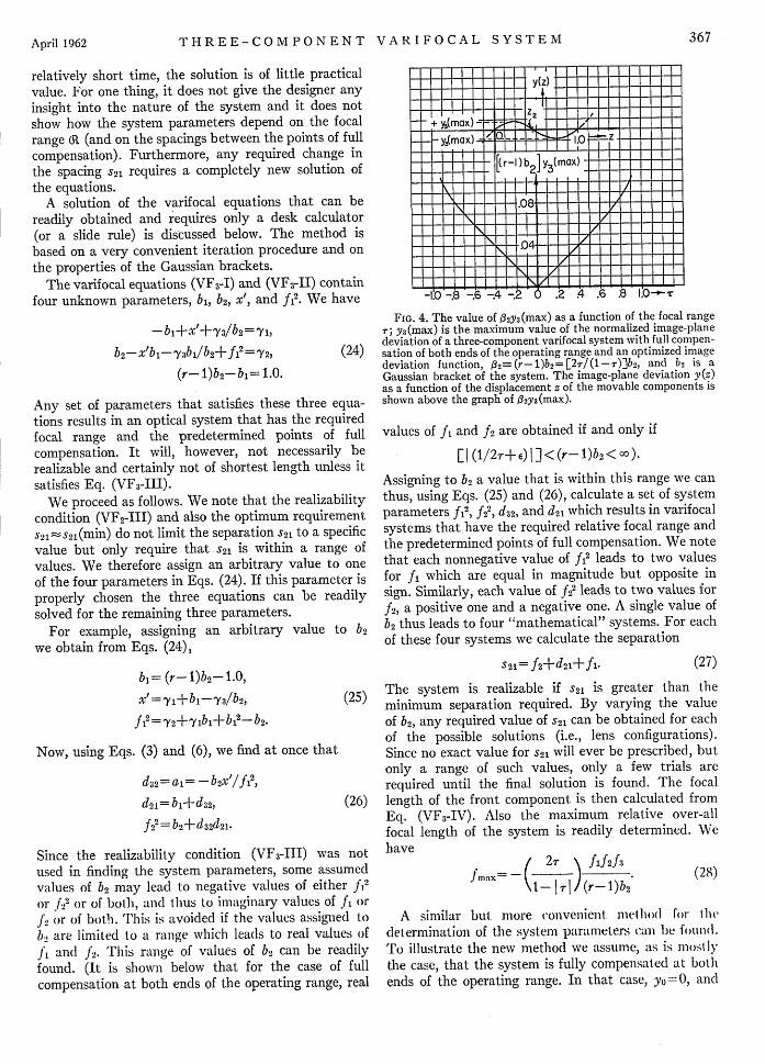
FIG. 4. The value of 32y3 (max) as a function of the focal range7; y3(max) is the maximum value of the normalized image-planedeviation of a three-component varifocal system with full compen-sation of both ends of the operating range and an optimized imagedeviation function, 3,B2(r-1)b2=[2/(1-)]b2, and b2 is aGaussian bracket of the system. The image-plane deviation y(z)as a function of the displacement z of the movable components isshown above the graph of ,32 y3(max).
values of fl and f2 are obtained if and only if
E l (1/2,+,e) | ] < (r- I)b2 < ) .
Assigning to b2 a value that is within this range we canthus, using Eqs. (25) and (26), calculate a set of systemparameters f12, f22, d32, and d2l which results in varifocalsystems that have the required relative focal range andthe predetermined points of full compensation. We notethat each nonnegative value of f12 leads to two valuesfor fl which are equal in magnitude but opposite insign. Similarly, each value of f22 leads to two values forf2, a positive one and a negative one. A single value ofb2 thus leads to four "mathematical" systems. For eachof these four systems we calculate the separation
S21= f2 +d 2 l+fl- (27)
The system is realizable if s21 is greater than theminimum separation required. By varying the valueof b2, any required value of s21 can be obtained for eachof the possible solutions (i.e., lens configurations).Since no exact value for s21 will ever be prescribed, butonly a range of such values, only a few trials arerequired until the final solution is found. The focallength of the front component is then calculated fromEq. (VF3-IV). Also the maximum relative over-allfocal length of the system is readily determined. Wehave
- 2( \ flf2 3
\-1=-t1|T|/(r-)b2'(28)
A similar but more convenient mellod for thledetermination of the system parameters can be fomud.To illustrate the new method we assume, as is mostIVthe case, that the system is fully compensated at bothends of the operating range. In that case, yo=O, and
367 April 1962
-I U _.t _.(0 _., -.- U . -It .0 ,. -k "
LEONARD BERGSTEIN AND LLOYD MOTZ
(x)-1
= m +0'
Ihm 2(A)
4lm I I - -_
3lm -1 4- I 1 [Ii 1 21ml-" .- I
ml -
I , -
(B2)p or(-I32)N
(fI Por(f I)N
2-Zlml[-lml Cft wtlm.,k-j2lml 31m`- T'2
C-.- I -- IIIII 1II (X)por(-X)N-I - ~~~~I ~
, -Im Region of_lrealizable Region of
2Iml 0 _ _ s~+NPN realizable-2ml Ssfems PNP
-31m I ( X 52>0) sse
l l _ _ Region of realizable-41mli PNPand NPN systems
l l
I , X C = (t(O))p or (I))
0.75 + - -2 1 s1
FIG. 5. The parameters f, f22, and 6l2 of three-comb
varifocal systems as functions of the parameter X, or of 1; f,focal length of the rear movable component, f2 is the focal Iof the stationary component, and 2= (r-1)b 2= [27/(1 -
where b2 is a Gaussian bracket of the svstem and r is the ncized focal range. The index P refers to P systems, the indexN systems. ()p=14'(O) and (I)Nv=-1j'(1), where 11'(O) a(1) are the normalized final image distances in the two expositions ( and 1.0) of the movable components; X 1
1'(0-(M-e) =l1'(l)+O.5- (n-e), where in-1/4(1/r+2e) an0.5-Z2 is given by Eq. (20) or Fig. 3. (r, in and e are pcfor P systems and negative for N systems.)
Eqs. (24) become
_-bl+x'=,Y = 1.5 - ,b2-xbi+fi2= Y = 0.5-,
(r- )b2-b = 1.
Let 1' (0) and 11' (1) denote the normalizedimage distances measured from the rear prinplane of the rear movable component in its frorrear positions, respectively, and let
Using Eqs. (26) and (27) we then calculate the param-eters d32, d21, f22, and 21. The system is realizable iff2
2 is positive and 21 is larger than s21(min).We will now find the range of values of I or of X which
lead to real values of f2. Expressing 22 in terms of Xwe obtain
4(m- )X(X+m)2- (1-4e2 )X2
f2 2= (-m)(37)
We note from Eq. (37) that f22 is positive and thus f2 realif and only if X is positive for P systems and negativefor N systems, i.e., if
(XN)p>O and (-x)N>0,or (38)
length 1> (3(R-1)/4((R-1)-' le
rNrtl In Fig. 5, fl, f22, and 2 are shown as functions of Xnd 11 and I for the region in which realizable solutions exist.treme We observe that the plots of (fi)p and (2)p as functionsad, e- of I or ()p are identical with the plots of (-fl)N andIsitive (-132)Nv as functions of I or (-X)N. We also note that
1121 >21in ='(&+1)/((R-1)+ eI.Assigning values to I which are within the realizable
range, and using Eqs. (31), (33), (34), (35), (36), (26),and (27), a set of parameters is readily found which
29) will result in a system having the predetermined focal) range 61 with the chosen spacing s21. The system will
be a P system if r (or X) is assumed positive and an Nfinal system if (or ) is assumed negative. In each case acipal number of different lens configurations are possible.cipar We consider first the P system. It is readily found
tt or that for any operating range three different lenssystems are possible.
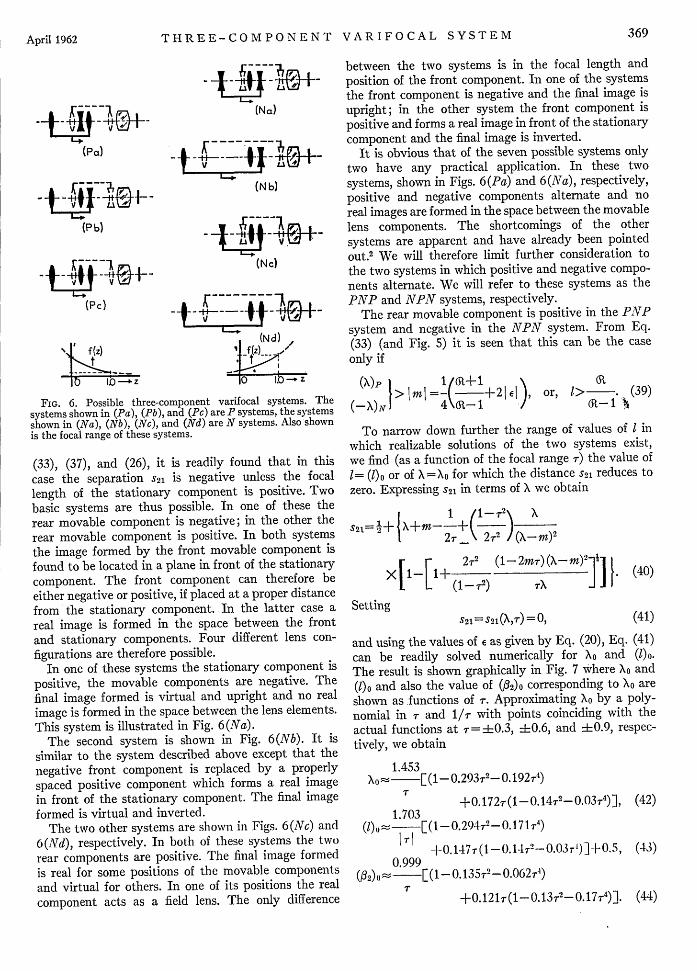
In one of these systems the movable components are(30) positive and the stationary component is negative. The
final image formed is real and inverted and no realimage is formed in the space between the movable lenselements. This system is shown in Fig. 6(Pa).
(31) The other two systems are illustrated in Figs. 6(Pb)and 6(Pc), respectively. In one of the systems the two
the front components are positive and the rear componentis negative, and in one of the systems all three compo-
(32) nents are positive. I both systems a real image isformed in the space between the two movable compo-
it if nents. The final image formed is real and inverted ila; one of the systems and real and upright in the other.
ims.) We now consider the N1T systems. Using Eqs. (27),
368 Vol. 52
I
369THREE-COMPONENT VARIFOCAL SYSTEM
(Pa)
(P b)
(Pc)
1( +z)
I D - _~
(Na)
(Nb)
(Nc)
FIG. 6. Possible three-component varifocal systems. Thesystems shown in (Pa), (Pb), and (Pc) are P systems, the systemsshown in (Na), (Nb), (Nc), and (Nd) are N systems. Also shownis the focal range of these systems.
(33), (37), and (26), it is readily found that in thiscase the separation s21 is negative unless the focallength of the stationary component is positive. Twobasic systems are thus possible. In one of these therear movable component is negative; in the other therear movable component is positive. In both systemsthe image formed by the front movable component isfound to be located in a plane in front of the stationarycomponent. The front component can therefore beeither negative or positive, if placed at a proper distancefrom the stationary component. In the latter case areal image is formed in the space between the frontand stationary components. Four different lens con-figurations are therefore possible.
In one of these systems the stationary component ispositive, the movable components are negative. Thefinal image formed is virtual and upright and no realimage is formed in the space between the lens elements.This system is illustrated in Fig. 6(Na).
The second system is shown in Fig. 6(Nb). It is
similar to the system described above except that thenegative front component is replaced by a properlyspaced positive component which forms a real imagein front of the stationary component. The final imageformed is virtual and inverted.
The two other systems are shown in Figs. 6(Nc) and6(Nd), respectively. In both of these systems the tworear components are positive. The final image formedis real for some positions of the movable componentsand virtual for others. In one of its positions the realcomponent acts as a field lens. The only difference
between the two systems is in the focal length andposition of the front component. In one of the systemsthe front component is negative and the final image isupright; in the other system the front component ispositive and forms a real image in front of the stationarycomponent and the final image is inverted.
It is obvious that of the seven possible systems onlytwo have any practical application. In these twosystems, shown in Figs. 6(Pa) and 6(Na), respectively,positive and negative components alternate and noreal images are formed in the space between the movablelens components. The shortcomings of the othersystems are apparent and have already been pointedout.2 We will therefore limit further consideration tothe two systems in which positive and negative compo-nents alternate. We will refer to these systems as thePNP and NPN systems, respectively.
The rear movable component is positive in the PNPsystem and negative in the NPN system. From Eq.(33) (and Fig. 5) it is seen that this can be the caseonly if
or, I1> 6 . (39)i-1 To narrow down further the range of values of I in
which realizable solutions of the two systems exist,we find (as a function of the focal range r) the value ofI = (1)o or of X = Xo for which the distance S21 reduces to
zero. Expressing s21 in terms of X we obtain
1 -2] XS21= 2+ +
2T _ 2T2 (X M)2
r 1r 2T2 (1-2m)(1<_M)1 (40
X |1 L +(1- 2) TX ]| .(0
SettingS21 = S21(X,T) = 0, (41)
and using the values of e as given by Eq. (20), Eq. (41)can be readily solved numerically for Xo and (.The result is shown graphically in Fig. 7 where Xo and(l)o and also the value of (32)0 corresponding to Xo areshown as functions of T. Approximating Xo by a poly-
nomial in 7 and 1/T with points coinciding with theactual functions at r=J-0.3, h0.6, and 4-0.9, respec-tively, we obtain
FIG. 7. The values of the parameters ()o, Xo, and ()o of theoptimum three-component varifocal systems as functions of thefocal range ; ()o, Xo and (12)0 are the values of , X and 2 [2r/(1 -)]b 2 for systems in which the distance S21 between theprincipal planes of the stationary component and the rear movablecomponent in the position z 0 is zero.
Realizable solutions areX>X0, or when
()OP <1= 11'(0) < oo,and
61-<1=-11 (1)< (ONX
thus obtained only when
for the PVP system,
for the NPN system,
with S21 =° when = (I)o.The region of realizable PNP and NPN systems is
indicated in Fig. 5. The value of (I)o for PNP systems is,as can be seen from Eq. (43), larger than the value of(l)o for NPN systems, that is, ()op> ()oN. Further-more, an increase in ()o will result in an increaseof 21 for P systems, whereas a decrease in (l)o isnecessary in order to increase the value of 21 for Nsystems. It is also seen from Eq. (40) that the sameabsolute value of X that gives S21= 0for P systems willgive S21= +1.0 for N systems and vice versa.
Optimum systems are obtained when the spacing s21has the physically smallest possible value, i.e., close tozero. The powers of the individual components arethen oflapproximately the same order of magnitude,the sum of the lens powers is nearly zero and the lenssystem has the smallest possible physical dimensions."
1 The choice between the two optimum systems is governed bya number of considerations. 2 (The PP system is generallypreferable.)
Vol. 52
For the two optimum systems, to which we shallrefer as the (PNP)o and (P.V)o systems, respectively,the value of I which results in a predetermined value ofS21 will thus differ only slightly from ()o. Only two orat most three trials are thus necessary to determine thesystem parameters from Eqs. (31), (33), (34), (35),(36), (26), (27), and (VF 3-IV). On a conventionaldesk calculator this takes no more than five to tenminutes.
Instead of using a trial and error method for deter-mining the system parameters for a given focal range aR,it is often found more convenient to plot, using Eq. (40)and values of e as given by Fig. 5 or Eq. (20), the spacingS21 as a function of I for values of I located within therange given by Eq. (44). From the plot, the value of Icorresponding to any specified value of 21 can bedetermined and the system parameters calculated fromEqs. (31), (33), (34), (35), (36), (26), (27), and(VF3-IV). This has the advantage that design changescan be readily made.
An example illustrating the method described aboveis given in this paper.
4. Focal Lengths of the Components, Final ImageDistance, Maximum Over-All Focal Length,
and Maximum Image-Plane Deviationof the (Optimum) Three-Component
Varifocal Systems
In the preceding section the values of the parametersXo and (I)o were found which result in P.VP and NPXsystems having a separation 21 -O between theprincipal planes of the stationary component and therear movable component in its original position. Foroptimum systems 21 is close to zero and the correspond-ing values of X and I differ only little from Xo and ()o.The same is also true for the system parameters fl, f2,and [f3- (s32 - 1.0)]. Their values for the optimumsystems differ only little from the values of (fl)o, (f2)0,and (f3)0l they assume when 21=0, where
(f3)0=(f3)0-(s 32 -1.0) = 1.0-(d 32)0-(f2)0 (46)is the focal length of the front component for the casewhen 21=° and the distance 32 between the principalplanes of the front and the stationary components hasthe smallest possible value under the assumption ofnegligible component thicknesses, i.e., 32=1.0. (fi)o,(f2)0, and (f3)0l thus give approximate values for thefocal lengths of the individual components of the twooptimum systems.
The values of (fl)o, (f2)0, and (d32)0 have already beenfound in solving Eq. (41) for X0. Using Eq. (VF 3-IV)also, (f3)0l is readily calculated. The results are showngraphically in Fig. 8, where (fl)o, (f2)0, and (f)o, areshown as functions of the focal range. These functionscan be closely apl)roximated by polyfloniials in and1lT with the dominant term proportional to 1/r.Approximating (fl)o, (f2)0, and (f3)0l by polynomials
370
- 1 11
T
_ i .P
201
r rt
(X)0
(X)o
0'2)0-,,,, . ,,I1,
. - . . . .. . . .
II I I if - - 11-7'- -4
2-1:(5.-..B -. 6 -. 4--.2 -
Ld-212I~_ l_v ia
I "
THREE-COMPONENT VARIFOCAL SYSTEM
in and l/r with points coinciding with the actualfunctions at -= ±0.3, 0.6, and 0.9, respectively,we obtain
0.704(fj)oz + [(1-0.313r2-0.26 7r4)
T+0. 184r (1- 0.14r2+0.10'r)],
0.704(f2) oz: - -[ (I-0.277 2_0.239r4)
T-0.184r(1-0.01r2+0.32r4)],
and1.704
(f3)0 Z + [(1-0.21OT2 0.146r4)r
+0.147r (1-0. 10r2- 0.06r4)].
(47)
(48)
(49)
For P systems f3 is positive and (f3)0> (f3)0l, whereasfor N systems f3 is negative and (f3)01 < 1 (j3)011.It should also be noted that f> (fi)o, f2> (f2)0, andf3< (f3)o0.
The final image distance is given by Eq. (31). Thus,when 21 = 0, [11' (0)]o= Xo+0.5+ (0.25/r)-(1/2)e andcan be readily calculated (using the values of and X0
found previously) as a function of the focal range.The result is shown graphically in Fig. 8. Using theapproximate expressions for e and Xo as given by Eqs.(20) and (42), respectively, we obtain
1.703[1j'(0)]o~- [(1-0.294r2- 0.171I 4)
+0.440r (1-0.05r-20.01Ir4)]. (50)
The maximum over-all focal length of the system isgiven by Eq. (28). Thus, when s21 =0, and S32=1.0,
(fmax)01= -[2/(1- r) I ][(l)o(f2)o()(f3)01(2)O]
Using the values of (fl)o, (f2)0, (f3)0, and (02)0 foundpreviously, (fmax)oj can be readily calculated as a
function of the focal range. The result is shown graph-ically in Fig.-8. To the first approximation (fl)o, (f2)0,(o3)0l, and (02)0 are each proportional to l/r. Therefore,to the same order of approximation, (fmax)ol 1/r.Approximating (fmax)o, by a polynomial in r and l/r,with points coinciding with the actual function atr ±0.3, ±40.6, and ±-0.9, respectively, we obtain
2.075(fmax)oli [(1+0.884r2+0.808r4)
r
+0.022r(1+2.34T2-3.36r4)]. (51)
The product of ,B2 and the maximum value of thenormalized image deviation function was foundpreviously. Under the assumption of S21=0 we thusobtain
y(max)o= [022y(max)]/(2)0. (52)
The image-plane deviation of the complete varifocalsystem (including the auxiliary component) is given2
(f)[ o(O3.
4d()YO
rtfI
(fOI
,fmax) 0
e1(°)]o
(f3 )o(f)o
FIG. 8. The normalized focal lengths (fl)o, (f2)0 and, (f3)01 ofthe components, the final image distance [1'(0)]o and the normal-ized maximum over-all focal length (fmaxc)oi of the optimum three-component varifocal systems as functions of the focal range T.The index 0 indicates that the particular parameter was foundunder the assumption that S21 = 0, the index 01, that the parameterin question was found under the assumption that S21=0 andS32= 1.0; S21 and S32 are the distances between the principal planesof the components 2 and 1, and 3 and 2, respectively, in theposition z= 0 of the movable components.
by YT(Z) = [FT2(max)/Zm.]e(z), where e (z) y(z)/fmax2 and FT(max) is the maximum over-all focal
length of the complete system. Assuming S21=0 ands32= 1.0 we thus obtain
YT(max)ol y(max)o ( 1r)23 0(max) o = =
FT2(max)/Zm (fmax)o12 4 r2
/ (32)oD32y(max)] . (53)
[ (f1) 0 (f2) 0 (f3) 01]2
Using the values of [02y(max)], (,B2)0, and (fma-,)oj asfound previously, y(max)o and (e(max)0 l are readilycalculated. The results are shown in Figs. 9 and 10,respectively, where y(max)o and E)(max)ol are shownas functions of the focal range. To the first approxima-tion, [ 2y(max)]-0.09 4 r, (02)0-0.999/r, and (fma)0i-2.075/r. Therefore, to the same order of approxima-tion, y(max)o- (0.094/0.999)r2 = 0.09472, and G (max)oi~-[0.094/ (2.075)2]r4 =0.0218r4. Approximating y(max)o
and E)(max)0 l by polynomials in T starting with I2 andT4, respectively, and with points coinciding with theactual functions at r=4±0.3, ±t0.6, and ±0.9, respec-
F-T-7 -T I
I - I I I | I I I 1'# 1 1 1 fl .
l l l l l
I I, | I | I ! 1- l F I ~1r 1-t I I I f I I I '
T/-TTT1/ I I I
INA
J, I I I
I-L
371April 1962
40#2#4P61#8
3
7 ti9 L
4_ s _HIO
LEONARD BERGSTEIN AND LLOYD MOTZ
_I 31111 111 11
- - , I I
.040--
.020---
-I. S.0 - -. It -.S U . .0 .0 U-T
FIG. 9. The maximum value y3(max)o of the normalized image-plane deviation of the optimum four-component varifocal systemswith full compensation at both ends of the operating range (andan optimized image deviation function) as a function of the focalrange T. The distance 21 between the principal planes of thestationary and rear movable components in the position =0 isassumed to be zero.
The maximum value of the image-plane deviation isthus, assuming optimum conditions, almost uniquelydetermined by the relative focal range of the system,
FIG. 10. The maximum value YT(max)oi of the image-planedeviation of optimum three-component varifocal systems withfull compensation at both ends of the operating range (and anoptimized image deviation function) as a function of the focalrange r. The distances between the principal planes of the compo-nents in the position z=0 are assumed to be S21=O and S 2 = 1.0,respectively. FT(max) is the maximum over-all focal length ofthe system and Z is the maximum displacement of the movablecomponents.
the maximum over-all focal length, and the maximumdisplacement of the movable components. In contrastto two-componenI. systems, the ' system has a smallerimage-plane deviation than the N system of the samefocal range (R. However, the difference is relativelysmall.
III EXAMPLE
Let it be required to design a varifocal objective withan over-all focal length varying continuously between33.33 and 100.00 mm.
As the first step in the design we estimate the smallestvalue of the maximum image-plane deviation YT (max)that can be obtained with a three-component varifocalsystem.
The focal range of the system is a1= FT(max)/FT(min)=3.0, and T| (61-1)/(61+1)=0.5. FromFig. 10 or Eq. (55) we find that if a P system is used(T= +0.5),
e (max)o 1 = 0.00082,and
YT(max)ol= (0.00082)FT2 (ma x)/
and if an N system is used (T= -0.5),
0 (max)o1 = 0.00096,and
YT (max) 0 = .00096FT (max)/Z m.
Choosing Zm=40.0 mm for the maximum displacementof the movable components we obtain, with FT(max)= 100.00 mm,
[yT(max)ol]p= 0.21 mm,and
[yT(max)ol]N=0.24 mm.
Assuming that these values are within the maximumpermissible value we can proceed with the design. Weshall consider both, PP and NPN, optimum systems.
The approximate values for the thin lens parametersof the two optimum systems are found at once. Usingthe results of Fig. 8 or of Eqs. (47)-(51), we find thatthe focal lengths of the three components of the(PNP)o system (T=+0.5) are
(FI)o= + (1.400) (40.00) mm = +56.00 mm,
(F2)0 -(1.154) (40.00) mm= -46.16 mm,and
(F3 )01= + (3.436) (40.00) mm= + 137.44 mm.
The maximum over-all focal length of the variablefront system is
The parameters (fl)o, (f2)o, (fB)o, and the values of(fmax)ol and 11'(0)]o are found for the case when theseparations between the components have the smallestpossible values under the assumption of negligiblecomponent thicknesses, i.e., when S21=0 and S32=1.0.
In the actual case the finite thicknesses of the compo-nents (i.e., the finite distances between the principalplanes and the corresponding component boundaries)must be taken into account and the separations mustbe larger than the minimum values required. We willnow proceed to find the actual values of the parametersof the two optimum systems.
We shall first consider the (PNP)o system. We have
(r)p=(R=3.0, and (r)p=+0.5.
Assuming that the system is fully compensated at bothends of the operating range we find from Fig. 5 orEq. (20) that for T= +0.5,
stationary and the rear movable components is ()o=3.859. We will therefore, using Eqs. (31), (33)-(36),(26), (27), (VF3 -IV), and (28), calculate the Gaussianparameters of the system for I= (l)o= 3.859, (1) = 3.910,(1) = 3.960, and (1) = 4.010, respectively. The resultsare shown in the first four columns of Table I.
In Fig. 11 (a) the separation S21 is plotted as a functionof I for 3.859= (l)o<1<4.010. [Note the almost linearrelation between S21 and ()o.] For any desired value ofS21 the corresponding value of (1) is thus readily foundfrom the graph or from the calculated values byinterpolation. We shall assume that a distance ofapproximately 6.0 mm is sufficient to account for thefinite thicknesses of the components of the varifocalsystems proper. Setting s2j=0.15(=6.0/40.0) we findthat the corresponding value of I is 3.9404. Using thisvalue of I and assuming s32= 1.15, the system parametersare readily calculated. This is shown in the fifth columnof the above table. The parameters of the system arethus
f3= +3.5205,]
S32= 1.1500,
f2= - 1.1199,S21= 0.1500,
fi = + 1.4413,J
or, with
Zm= 40.0 mm,
F3= + 140.82 mm,
S32= 46.00 mm,
F2= -44.80 mm,S21= 6.00 mm,
F1 =+57.65 mm.
e= 0.080.
The points of full compensation are thus located at
Z1 =0, Z2==0.420, Z3=1.00.
This gives
andyl= 1.420, 'Y2=0.420, 73=O,
m = (1/2T+ e) = 0.540.
From Fig. 7 or Eq. (42) we find that for = +0.5 thevalue of the parameter I that results in a system with adistance S21=0 between the. principal planes of the
(NPN SYSTEM) z .4
I
2''_1 I I A11LI1
3.6 196 '- --3.41 -3.31 '-3.;1 -. 1
Fic. 11. The distance 21 between the principal planes of thestationary and rear movable components as a function of theparameter I for the two three-component systems of the exampleof Sec. III.
fm.. = 2 ( f I f2| f3| )/fl2 -5.0257 -5.3076 -5.5226 -5.7876 -5.3051
It should be noted that none of the focal lengths differsby more than 3% from the approximate values foundpreviously under the assumption that 21= 0 ands 32 = 1.0.
The final image distance of the front system is
L1'(z)> (3 .94 04-z)40.0 mm= (157.62-40.0z) mm,
and the over-all focal length is given by
F(z) =5.4661
1+1.0381z+0.9619z2-40.0 mm.
The objective is to have an over-all focal lengthvarying from FT(max)= 100.00 mm to FT(min)= 33.33mm. The auxiliary system must therefore reduce thefocal length of the front system by a factor
W= (5.4661) (40.0)/100.0= 2.1864.
The auxiliary system will be a composite systemcomprising a number of lens elements. We thereforechoose So= (1.30) (40.0) mm= 52.00 mm. This givesLo= 105.62 mm. The focal length of the auxiliarysystem becomes Fo= (105.62/1.1864) mm=89.02 mm,and the final image distance is Lor= (105.62/2.1864)mm=48.31 mm. The physical length of the system isS= (2.60) (40.00) mm= 104.00 mm= 1.04 FT(max), andthe over-all distance between the front component andthe image plane is L=S+Lo'= 152.31 mm=I.523FTX (max).
The image-plane deviation of the objective is given by
- z(z- 0.420) (z- 1.000)-Y2'(Z)=250.0 0.0322' mm.
_ 1+1.0381z+0.9619z 2 1
The maxima of YT(z) are located at Z1.2=0.17 andz 2, 3 = 0.72, and the corresponding values of the maximaare Y(max) = 0.24 mm and 0.22 mm, respectively. Thevalues of the two maxima thus differ only little fromeach other and are close to the value of 021 mm givenby Eq. (55).
Assuming that the objective is to have a relative
aperture of 0.25 and is to cover a field varying from240 (in position of minimum over-all focal length) to 8°(in position of maximum over-all focal length) we findthat the diameters required for the aperture are(Dia3)A=25.00 mm, (Dia2)A=16.84 mm, (Dial)A=18.03 mm, and (Diao)A=12.08 mm, and that thediameters required for the field are (Dia 3 )F= 28.70 mm,(Dia2)F=12.90 mm, (Dial)F=12.60 mm, and (DiaO)F- 1.65 mm, respectively.
We shall now consider the (I\TPAT)o system. Now,(r)N= 1/R= , and r= -0.5. Assuming, as before, fullcompensation at both ends of the operating range, wenow have e = - 0.080, and the points of full compensa-tion are located at z = , Z2= 0.580, Z3 = 1.000. This givesy1= 1.580, 2=0.580, 3=0, and m=-0.540. FromFig. 7 or Eq. (42) we now find that (I)o=3.377. Wetherefore now calculate the Gaussian parameters ofthe system for () = ()o= 3.377, 1= 3.310, 1= 3.260, and1=3.210, respectively. The results are shown in thefirst four columns of Table II.
In Fig. 11 (b) the separation S21 is plotted as afunction of l'(1)=-l, for -3.377=-(I)o<-I<-3.210. Assuming, as before, that 21 =0.15 we findthat the corresponding value of I is -3.3106. Theparameters of the varifocal system for this value of Iand s32= 1.15 are shown in the fifth column of Table IIWe obtain
Li'(z) - [3.3106- (1.0-z)]40.0 mm= -[132.42-40.0(1.0-z)] mm
F() = -5.3051/(3-3.1253z+1.125352)]40.0 mm.
We note again that none of the parameters differs by
374
THREE-COMPONENT VARIFOCAL SYSTEM
f, M~ir I
8.05z(z-0.42) (z- 1.00)1.0+1.0381z+0.96l9z 2
-.20 11111 + 1
FT (Z) = 100.01.0 +1. 03 81z+0.9 6 9zmm
10.OOz(z-0.58)(z- 1.00)3.0-0.1253z+1.125 3 z' mm
- I-th4IIE I II
-. 10
-.30
FT (Z) =
4 H 1-1 81' Il
L_
100.0)-3.125 3z+1.1: 53Z2MM
4 .6 . 10 Z
SYSTEM
100
50
333
4
4Z
U .2 .4 ' -
NPN SYSTEM
FIG. 12. The two optimum three-component systems of the example of Sec. III, andtheir image-plane deviation and focal range.
more than 3% from the approximate values foundpreviously under the assumption that 21= 0 ands32= 1.0.
The reduction factor of the auxiliary system is now
W= - (5.3051)(40.0)/100.0=: -2.1220.
Choosing, as before, Slo=52.00 mm, we obtain Lo=-144.42 mm, and consequently FO= +46.26 mmand Lo'= +68.06 mm. The physical length of thesystem is S= 104.00 mm, the same as that of the(PNP)o system, and the over-all distance between thefront component and the image plane is
L= 172.06 mm.= 1.72FT(max).
The image plane deviation of the objective is given by
The maxima of YT(Z) are located at Zl,2=0.29 andz2,3= 0.79 and the corresponding values of the maximaare YT(max) = 0.27 mm and 0.30 mm, respectively.
We see again that the values of the two maxima differonly little from each other and are approximately equalto the value of 0.24 mm given by Eq. (55).
Assuming that the objective is to have a relativeaperature of 0.25 and is to cover a field varying from24° to 80, we find that the diameters required for theaperature are (Dia3)A= 25.00 mm, (Dia2)A= 26.30 mm,(Dial)A= 15.60 mm, and (DiaO)A= 17.02 mm, and thatthe diameters required for the field are (Dia3)F= 22.70mm, (Dia2)F= 12.46 mm, (Dial)F=9.85 mm, and(DiaO)F= 1.29 mm, respectively.
Both systems, the (PNP)o and (NPN)o, are shownschematically in Fig. 12. Also shown in the same figureare the focal range and the image-plane deviation ofthe two systems.
CONCLUSION
The theory presented in this paper enables one todetermine the optimum Gaussian parameters of athree-component optically compensated varifocal systemalmost at a glance. The problem of correction of theimage aberrations of the system over its entire operatingrange will be discussed in a forthcoming paper.