University of Rhode Island University of Rhode Island

DigitalCommons@URI DigitalCommons@URI

Open Access Master's Theses

2014

THREE-DIMENSIONAL TOPOLOGY OPTIMIZATION OF THREE-DIMENSIONAL TOPOLOGY OPTIMIZATION OF

STATICALLY LOADED POROUS AND MULTI-PHASE STRUCTURES STATICALLY LOADED POROUS AND MULTI-PHASE STRUCTURES

Matthew Okruta University of Rhode Island, matthew_okruta@my.uri.edu

Follow this and additional works at: https://digitalcommons.uri.edu/theses

Recommended Citation Recommended Citation Okruta, Matthew, "THREE-DIMENSIONAL TOPOLOGY OPTIMIZATION OF STATICALLY LOADED POROUS AND MULTI-PHASE STRUCTURES" (2014). Open Access Master's Theses. Paper 347. https://digitalcommons.uri.edu/theses/347

This Thesis is brought to you for free and open access by DigitalCommons@URI. It has been accepted for inclusion in Open Access Master's Theses by an authorized administrator of DigitalCommons@URI. For more information, please contact digitalcommons@etal.uri.edu.

THREE-DIMENSIONAL TOPOLOGY OPTIMIZATION OF STATICALLY

LOADED POROUS AND MULTI-PHASE STRUCTURES

BY

MATTHEW OKRUTA

A THESIS SUBMITTED IN PARTIAL FULFILLMENT OF THE

REQUIREMENTS FOR THE DEGREE OF

MASTERS OF SCIENCE

IN

MECHANICAL ENGINEERING AND APPLIED MECHANICS

UNIVERSITY OF RHODE ISLAND

2014

MASTER OF SCIENCE THESIS

OF

MATTHEW OKRUTA

APPROVED:

Thesis Committee:

Major Professor David G. Taggart

Carl-Ernst Rousseau

Frederick J. Vetter

Nasser H. Zawia

DEAN OF THE GRADUATE SCHOOL

UNIVERSITY OF RHODE ISLAND

2014

ABSTRACT

A novel topology optimization method called Prescribed Material

Redistribution (PMR) has been under development at the University of Rhode Island

for the past several years. Originally implemented through a series of Fortran

subroutines used in conjunction with the commercial finite element package, Abaqus,

a standalone two-dimensional Matlab code was developed and used in evaluating the

method. In order to explore the capabilities of the PMR scheme for three-dimensional

problems, it became necessary to develop a three-dimensional version of the PMR

Matlab code.

The objective of this thesis, therefore, is the development and evaluation of a

three-dimensional Matlab implementation of the PMR scheme. The code allows users

to analyze general topology optimization problems by defining an appropriate design

domain, load conditions, support conditions, predefined fully dense or void regions,

and symmetry conditions. The code also provides the capability to impose constraint

conditions where coupling of displacement degrees of freedoms can be specified by

the user. A primary aspect of this work is the development and implementation of

hexahedral finite element equations. Since three-dimensional problems can be

computationally intensive, the finite element analysis implementation includes

computationally efficient algorithms where feasible. The post-processing phase of the

analysis included the generation of optimized three-dimensional geometry in the

standard STL file format. The STL file allows users to examine the results using

standard CAD file viewers. Also, the STL file can be used as input to additive

manufacturing equipment such as 3-D printing for the manufacture of physical

components.

The three-dimensional PMR code is evaluated by two types of optimization

problems. The first set of test cases investigated are based on the identification of a

known topology for a centrally loaded, simply supported beam. Although this

problem can be considered using a two-dimensional analysis, performing a three-

dimensional analysis allowed for the ability to consider several different symmetry

cases. This is useful for evaluation of the symmetry capabilities of the three-

dimensional PMR code. For the symmetry case where all three coordinate axes define

symmetry place, an alternate test case was developed and used for evaluating the code.

The second set of test cases were designed to identify optimal topologies for two-

phase composite microstructures under general three-dimensional stress states. By

defining unit cell models with appropriate loading and constraint conditions, any

three-dimensional stress states can be modeled. If one of the composite phases is

taken to have essentially zero stiffness, this approach can be used to determine the

optimized microstructure of porous materials. Several test cases are evaluated for the

identification of optimized microstructures for both porous and composite materials.

iv

ACKNOWLEDGEMENTS

Foremost, I would like to express my sincere gratitude to my graduate advisor

Professor David Taggart for the continuous support of my Master’s Thesis research

over the past two years. His willingness to provide assistance at all times and

understand my struggles throughout the journey are greatly appreciated, and I could

not have asked for a better advisor and mentor.

I would also like to thank the professors on my Thesis Committee for

volunteering their own valuable time towards helping me complete my defense. These

individuals include Professor Carl-Ernst Rousseau, Professor Frederick Vetter, and

Professor Aaron Bradshaw.

And lastly I would like to thank my loving family for staying by my side the

entire time as I complete my graduate degree.

v

TABLE OF CONTENTS

ABSTRACT ................................................................................................................. ii

ACKNOWLEDGEMENTS ......................................................................................... iv

TABLE OF CONTENTS ............................................................................................. v

LIST OF TABLES ...................................................................................................... viii

LIST OF FIGURES .................................................................................................... ix

NOMENCLATURE ..................................................................................................... xii

CHAPTER 1 - INTRODUCTION

1.1 Motivation for Thesis .............................................................................................. 1

1.2 Goals for the Thesis ................................................................................................ 1

1.3 Structure of Thesis .................................................................................................. 2

CHAPTER 2 - TOPOLOGY OPTIMIZATION

2.1 Optimization History .............................................................................................. 5

2.2 Topology Optimization .......................................................................................... 6

2.3 Homogenization Based Optimization .................................................................... 7

2.4 Solid Isotropic Material with Penalization ............................................................. 8

2.5 ESO Algorithms ..................................................................................................... 10

2.5.1 Evolutionary Structural Optimization ................................................................ 11

vi

2.5.2 Bi-Directional Evolutionary Structural Optimization ........................................ 12

2.6 Numerical Problems .............................................................................................. 12

2.6.1 Checkerboarding ................................................................................................ 13

2.6.2 Mesh Dependence .............................................................................................. 15

2.7 Prescribed Material Redistribution ....................................................................... 16

CHAPTER 3 - FINITE ELEMENT ANALYSIS

3.1 Three-Dimensional Elements ................................................................................ 20

3.2 Coordinate Systems ............................................................................................... 22

3.2.1 Local Coordinate System ................................................................................... 23

3.2.2 Global Coordinate System ................................................................................. 25

3.3 Stresses and Strains ............................................................................................... 26

3.4 Shape Functions .................................................................................................... 29

3.5 Jacobian Matrix ..................................................................................................... 30

3.6 Strain-Displacement Matrix .................................................................................. 30

3.7 Stiffness Matrix ..................................................................................................... 31

3.7.1 Local Stiffness Matrix ........................................................................................ 32

3.7.2 Global Stiffness Matrix ...................................................................................... 32

3.8 Stress and Strain Calculations ................................................................................ 33

vii

CHAPTER 4 - THREE-DIMENSIONAL PMR CODE DEVELOPMENT

4.1 Matlab Introduction ............................................................................................... 34

4.2 Overview of Matlab Script .................................................................................... 35

4.2.1 Parameter Initialization ...................................................................................... 35

4.2.2 Finite Element Function ...................................................................................... 39

4.2.3 Symmetry Function ............................................................................................ 42

4.3 STL File Generation .............................................................................................. 44

CHAPTER 5 - ANALYSIS OF RESULTS

5.1 Symmetry Conditions ........................................................................................... 45

5.2 Microstructures ..................................................................................................... 50

5.2.1 Porous Microstructures ...................................................................................... 51

5.2.2 Composite Microstructures ................................................................................ 54

CHAPTER 6 - CONCLUSIONS AND FUTURE WORK

6 Conclusions and Future Work ................................................................................ 60

APPENDIX A - SYMMETRY TEST CASES ........................................................... 62

APPENDIX B - MATLAB SCRIPTS FOR SYMMETRY CASES ........................ 64

BIBLIOGRAPHY ........................................................................................................ 71

viii

LIST OF TABLES

Table 3.1 Node numbering and coordinate locations for local hexahedral element ... 25

Table 4.1 Predefined regions with corresponding node type and node densities ....... 36

Table 4.2 Matlab code translations for FE section ...................................................... 39

Table 4.3 Matlab translations and corresponding equations/tables for FE function ... 40

Table 5.1 PMR and STL time results for similar example using all eight symmetry

cases ............................................................................................................ 46

Table 5.2 Total CPU-time results for similar unique example using no symmetry

(Case 8A) and full symmetry (Case 8B and Case 8C) ................................. 48

Table 5.3 Stress values for each porous microstructure figure ................................... 51

Table 5.4 Stress values for each composite microstructure figure .............................. 55

ix

LIST OF FIGURES

Figure 2.1 Examples of (a) Size Optimization, (b) Shape Optimization and

(c) Topology Optimization [9] ................................................................... 7

Figure 2.2 Illustration of composite material made of a periodic

microstructure [10] .................................................................................... 8

Figure 2.3 SIMP flow chart [14] ................................................................................. 9

Figure 2.4 A catenary-type structure (a) Initial design (b)-(d) Evolution of

optimal shape [17] ..................................................................................... 11

Figure 2.5 (a) Design case, (b) Checkerboard example, (c) Solution for 600

element discretization, (d) Solution for 5400 element discretization,

(e) Non-unique example [9] ........................................................................ 13

Figure 2.6 Transition from initial to final relative density distribution for the case

𝜌0 = 0.3 [4] ................................................................................................ 18

Figure 2.7 Transition from initial to final cumulative relative density distribution for

the case 𝜌0 = 0.3 [4] .................................................................................. 18

Figure 3.1 Three common element types in three-dimensional analysis [24] ............. 21

Figure 3.2 Local coordinate system for a hexahedral element with appropriate nodal

numbering .................................................................................................. 24

x

Figure 3.3 Global coordinate system for multiple hexahedral elements with

appropriate nodal numbering. .................................................................... 26

Figure 3.4 Three-dimensional element under a state of stress [27] ............................ 27

Figure 5.1 Theoretical optimal Michell-Arch structure .............................................. 46

Figure 5.2 Michell-arch results using xy-symmetry for Case 6B ................................ 47

Figure 5.3 Initial conditions for Case 8 with full symmetry ....................................... 48

Figure 5.4 Full symmetry test cases results: Case 8A (top), Case 8 (middle)

and 8C (bottom) ......................................................................................... 49

Figure 5.5 Outline of unit cell model region ............................................................... 50

Figure 5.6 Unit cell model with constraints shown ..................................................... 51

Figure 5.7 Microstructures made of porous materials; (a) through (h) cases correspond

to conditions in Table 5.3 ........................................................................... 52

Figure 5.8 Two-phase composite microstructures; (a) through (g) cases correspond

to conditions in Table 5.4 ........................................................................... 55

Figure 5.9 3-D printed physical model of case shown in Figure 5.7(c) ....................... 58

Figure 5.10 3-D printed physical model of case shown in Figure 5.7(d) ...................... 58

Figure A.1 Michell-arch results using no symmetry for Case 1 ................................... 62

Figure A.2 Michell-arch results using x-symmetry for Case 2 ..................................... 62

xi

Figure A.3 Michell-arch results using y-symmetry for Case 3 ..................................... 62

Figure A.4 Michell-arch results using z-symmetry for Case 4 ..................................... 63

Figure A.5 Michell-arch results using xy-symmetry for Case 5 ................................... 63

Figure A.6 Michell-arch results using zx-symmetry for Case 6 ................................... 63

Figure A.7 Michell-arch results using yz-symmetry for Case 7 ................................... 63

xii

NOMENCLATURE

Acronyms:

AESO Additive Evolutionary Structural Optimization

AR Admission Volume Ratio

BC Boundary Condition

BESO Bidirectional Evolutionary Structural Optimization

CPU Central Processing Unit

DOF Degree of Freedom

ER Evolutionary Ratio

ESO Evolutionary Structural Optimization

FE Finite Element

FEA Finite Element Analysis

FEM Finite Element Method

LENS Laser Engineered Net Shaping

MRT Maxwell Reciprocal Theorem

PDE Partial Differential Equation

PMR Prescribed Material Redistribution

SIMP Solid Isotropic Material with Penalization

xiii

STL Standard Tessellation Language

Symbols

r, s Beta distribution parameters (Ch. 2)

β Beta function

βinc incomplete Beta function

x, y, z global coordinate notation

s, t, r local coordinate notation (Ch. 3)

z’ local coordinate notation used by Logan (respective to z in global)

𝛿 Delta function

u, v, w displacement parameters

[𝐶] elasticity matrix

Γ Gamma function

H Heaviside step function

[𝐽] Jacobian

J determinant of Jacobian

[𝐽]-1 inverse Jacobian

𝜌 relative density

𝜌0 initial relative density

xiv

𝜌𝑚𝑖𝑛 minimum relative density

N shape function

Ni shape function for ith node

𝜀𝑥, 𝜀𝑦, 𝜀𝑧 normal strains

𝛾𝑥𝑦, 𝛾𝑦𝑧, 𝛾𝑧𝑥 shear strains

[𝐵] strain-displacement matrix

𝜎𝑥, 𝜎𝑦, 𝜎𝑧 normal stresses

𝜏𝑥𝑦, 𝜏𝑦𝑧, 𝜏𝑧𝑥 shear stresses

[𝑘] local stiffness matrix

[𝐾] global stiffness matrix

VD final domain volume

Vf final structural volume

1

CHAPTER 1

INTRODUCTION

This introductory chapter will provide the reader with an overview of the

project. The structure of the thesis will then be outlined to provide efficient navigation

of the information and concepts discussed.

1.1 Motivation for Thesis

As the advancement in technology continues to grow with each passing

decade, the implementation of new and profound research to that technology has

become necessary. Companies are always searching for ways to design cost-effective

items and structures, while at the same time maintaining its proper functionality. The

growing field of topology optimization provides guidance for designers, and many

methods to date have been successful in optimizing the mechanical performance of

lightweight structures and components.

1.2 Goals of the Thesis

Previous work in the field of topology optimization has consisted of numerous

methods for the identification of minimum weight topologies. The Prescribed

Material Redistribution (PMR) scheme developed by Taggart and Dewhurst [1-5] has

been implemented in Matlab for a two-dimensional analysis using four-node

quadrilateral elements. This code identifies two-dimensional optimal topologies

which can be extruded in the third direction. Codes have been developed to represent

the extruded geometry in a 3-D STL file format. These models have been used to

produce prototypes on 3-D printing machines.

2

The thesis seeks to extend the Matlab script to include three-dimensional

analysis. The primary task is the implementation of a three-dimensional Finite

Element Analysis (FEA) solver in Matlab. Details of the 3-D formulation will be

presented in this thesis. Due to the computationally intense nature of 3-D analysis,

computationally efficient algorithms were implemented in order to minimize the run

time and memory requirements for each case. In addition to identifying techniques to

improve computational efficiencies within the script, the 3-D code allows the user to

impose half, quarter or one-eighth symmetry as appropriate for the particular structure

being modeled. The final script is applied to identify optimal porous and composite

material microstructures, depending on the given applied load conditions. For these

cases, the symmetry functionality plays a large role in efficiently modeling the

microstructure using appropriate unit cell models. Through post-processing mirroring

of the unit cell results, an array of desired size can be generated.

1.3 Structure of the Thesis

The field of topology optimization is an emerging field in the design

community and only recently is being incorporated in design software. This thesis

seeks to provide an overview of the field and details for a 3-D implementation of the

PMR method. The thesis contains six separate chapters which focus on different

aspects of topology optimization.

Chapter 2 presents a literature review of the field of topology optimization.

Major methods will be introduced, including the well-known SIMP and ESO

algorithms, as well as the more recent PMR scheme. It will be shown that these

methods have certain drawbacks, including common numerical problems such as

3

checkerboarding and mesh dependency. Techniques to limit or eliminate these

deficiencies will also be introduced.

Chapter 3 reviews the Finite Element Method, particularly as applied to three-

dimensional problems. A detailed formulation of the eight-node hexahedron element

is developed. For these analyses, a simple 3-D array of cube-shaped elements is used

to represent the design domain. A Cartesian coordinate system is employed with a

systematic node numbering scheme. Details of the element formulation and basic

stress and strain calculations are discussed, along with the main variables used in

three-dimensions. The shape functions, Jacobian matrices, strain-displacement matrix,

and stiffness matrices are then derived and shown in their proper equations. Terms

that require the use of both local and global recognition are separated into sections and

explained individually, such as the coordinate systems and stiffness matrices.

Chapter 4 discusses the Matlab code development. After a brief introduction

to the Matlab programming language, the key contents of the three-dimensional PMR

code will be discussed. These contents include an overview of the code formulation

and notations used, along with a brief definition of key aspects of the code.

Chapter 5 contains the results of several test cases that were used to evaluate

the code and to demonstrate its capabilities. The first main section explains the use of

symmetry conditions in the script for certain cases. The cases demonstrate the codes

ability to model various symmetry conditions and the corresponding computational

advantages. A table of CPU times demonstrating the effectiveness of running

symmetry functions is presented. The next set of test cases seek to identify optimal

4

microstructures for porous and composite materials that are subjected to various three-

dimensional multi-axial stress states.

Chapter 6 concludes the thesis with a summary of the main findings of the

research. Opportunities for future work associated with the project will be discussed.

5

CHAPTER 2

TOPOLOGY OPTIMIZATION

This chapter aims to provide an overview of the field of topology optimization,

including a literature review of recent contributions to this field. This review will

include work from the eighteenth century where optimization techniques first

originated, to the current twenty-first century where sophisticated optimization

techniques are becoming commonplace in many industries. The numerous methods

will be explained briefly, and the advantages and disadvantages will be discussed.

2.1 Optimization History

The existence of optimization methods can be traced as far back as the 1700’s

where prominent figures such as Newton, Cauchy, and Lagrange played a major role

in developing important work related to the field of optimization [6]. Despite these

theoretical contributions, development of practical optimization methods for use in

industry did not begin until the early 1900’s. In 1904, Michell [7] derived formulas

for minimum weight structures given different stress constraints and design domains.

These Michell structures, as they were known, marked the beginning of the

development of structural optimization methods. Later, in 1960, Schmit [8]

introduced a new approach to structural optimization that would serve as a basis to

many of the successful optimization methods used today. It was proposed that finite

element structural analysis and non-linear mathematical programming could be

combined to create optimal designs. The idea was considered revolutionary to many

in relation to design methods at the time, therefore it was pursued extensively over the

6

following decades. These developments were pursued in parallel with the rapid

growth of high-speed computers and the incorporation of finite element analysis in

computer-aided design.

2.2 Topology Optimization

By definition, the field of topology optimization is a mathematical approach

that optimizes a material structure in order to satisfy a given set of design

requirements. These requirements include the amount of material to be used in the

final design, the geometry of the design domain, boundary conditions (BC’s), and

applied loads. Typically, the amount of available material is to be distributed into

fully dense and void regions based on the results of the optimization within the design

domain. Many iterations are performed to reach the optimum design in computer-

aided software programs. Frequently, optimized designs are used in the conceptual

design process stage and then revised to further meet performance and

manufacturability standards. The advantage to incorporating topology optimization

into the design process leads to improved designs and the use of topology optimization

in many industries is expanding. Even if the design does not yield a result that can be

directly implemented, it does provide a benchmark optimal design that can be used to

evaluate more feasible designs.

Topology optimization is also referred to as layout optimization or generalized

shape optimization in many papers. Typically, two types of structures are considered:

continuum and discrete structures. Continuum structures often refer to single parts or

components, while discrete structures are typically larger structures such as trusses

and bridges.

7

Other forms of optimization analyses include size optimization and shape

optimization. An example of each type is clearly illustrated in Figure 2.1. In shape

optimization, the design parameters are considered and updated until the desired

constraints are achieved. This includes fillets, chamfers, radiuses, material thickness,

and many other design parameters. In size optimization, structures such as trusses and

bridges are considered and analysis is done on the bars supporting the inner portions

of the structure.

Figure 2.1: Examples of (a) Size Optimization, (b) Shape Optimization and (c) Topology Optimization [9]

2.3 Homogenization Based Optimization

The Homogenization Based Optimization (HBO) method was introduced in

1988 by Bendsøe and Kikuchi [9] and formed the basis for future topology

optimization schemes. In the method, a small unit cell structure is designed and then

homogenization is applied to determine the effective material properties of the

individual cells. As an example, the method recognizes periodic microstructures and

computes material properties of composites as demonstrated in Figure 2.2.

8

Figure 2.2: Illustration of composite material made of a periodic microstructure [10].

The unit cell to the far right is multiplied and shown in a 4 x 4 array in the center. The

material stiffness in this case is portrayed as a function of the microstructure and

density parameters [10].

𝐸 = 𝐸0(𝜌,𝜃, 𝜇… ) (2.3.1)

More recently, the HBO method has been replaced by a more effective method in

which the unit cell consists of a partially dense, solid isotropic region. This method,

called the Solid Isotropic Material with Penalization (SIMP) method, is described

below.

2.4 Solid Isotropic Material with Penalization

The Solid Isotropic Material with Penalization (SIMP) method was originally

introduced by Bendsøe [11] in 1989 and later developed independently by Rozvany et

al. [12] in 1991. In this method, each element in the finite element mesh is considered

to be partially dense. Through the course of several finite element iterations, the dense

regions are redistributed in order to minimize the overall compliance (or maximize the

overall stiffness) of the resulting structure. To inhibit the formation of regions with

intermediate partial density, a penalization scheme is implemented and requires a

heuristic penalization factor [13]. Due to SIMP’s ability to successfully identify

9

minimum weight topologies, it is widely used in the optimization field because of its

computational efficiency and simplicity.

The primary drawback of the SIMP method is the sensitivity of the results to

the penalty exponent, n, in the relation between local density, ρ, and Young’s modulus

𝐸 = 𝜌𝑛𝐸0, 0 ≤ 𝜌 ≤ 1 (2.4.1)

The parameter, n, refers to the amount of penalization. For n > 1, regions of

intermediate density have reduced density and are therefore penalized. This parameter

must be carefully selected to avoid results with an optimized structure containing

regions of intermediate density. The desired result is distinct regions of fully dense

material or regions with essentially zero density. In some cases, the user must explore

the effect of the penalization parameter on the resulting optimized structure.

The flow chart of the SIMP method provided in Figure 2.3 gives a general

overview of the procedure. The process begins with a uniform distribution of the

densities in all of the elements in the design domain, based on the desired volume

fraction specified by the user. A finite element analysis (FEA) is performed to

determine the mechanical response for the current material distribution. A sensitivity

analysis is applied to determine the relation between local element density and the

overall compliance of the structure. These sensitivities are used to update the element

densities for subsequent finite element iterations. To avoid numerical instabilities

such as checkerboarding, a filtering technique is implemented before updating the

element densities based on minimum compliance criteria. This entire process is

10

repeated until the structure converges to fully dense or fully void regions. The

converged structure represents the optimized design.

Figure 2.3 – SIMP flow chart [14]

In 2001, Ole Sigmund published an educational paper titled “A 99 line

topology optimization code written in Matlab” [15] that demonstrates both the

simplicity of the SIMP algorithm and the power of Matlab for use in topology

optimization problems. Using a highly efficient 99 line Matlab code, Sigmund

provides a complete compliance minimization scheme for use in identifying optimal

topologies in statically loaded two-dimensional structures. The code developed in this

study was initially based on Sigmund’s efficient 2-D topology optimization code.

2.5 ESO Algorithms

Evolutionary Structural Optimization (ESO) algorithms are based on the

simple concept that traditional structures are over-designed and therefore contain

regions that are stressed well below the corresponding material strength. For that

11

reason, improved designs can be achieved by removing unnecessary areas of dense

material. In ESO type optimization methods, iterative finite element analyses are

performed in which low stress regions are gradually removed from the structure. A

few of these methods are described below.

2.5.1 Evolutionary Structural Optimization

In 1992, Xie and Steven [16] developed a novel method of topology

optimization. The Evolutionary Structural Optimization (ESO) technique uses a finite

element based iterative scheme for removing inefficient, low-stress material from a

structure until an optimum design is reached. A common example of the ESO method

is the design of structures exhibiting only tensile or compressive regions. For

example, by identifying and removing the compressive regions in the structure, the

expected theoretically optimal catenary structure can be attained as seen in Figure 2.4

[17].

Figure 2.4: A catenary-type structure (a) Initial design (b)-(d) Evolution of optimal shape [17]

For the original method, once an element is removed from the structure, it could not be

restored. This limitation led to the Bi-Directional Evolutionary Structural

Optimization (BESO) method, which is discussed below.

12

2.5.2 Bi-Directional Evolutionary Structural Optimization

In 1998, Querin et al. [18] proposed the Additive Evolutionary Structural

Optimization (AESO) method that introduced the idea of material growth. When

combined with the ESO-algorithm, a new method emerged. The Bi-Directional

Evolutionary Structural Optimization (BESO) method allows for not only the removal

of material to eliminate low-stress, but also the addition of material to regions of high-

stress. The number of elements removed or added is determined by the evolutionary

ratio (ER) and the admission volume ratio (AR) [19]. To obtain the AR, the number

of elements added are divided by the total number of elements in the initial design.

Once the target volume of the structure is reached, the BESO algorithm is complete.

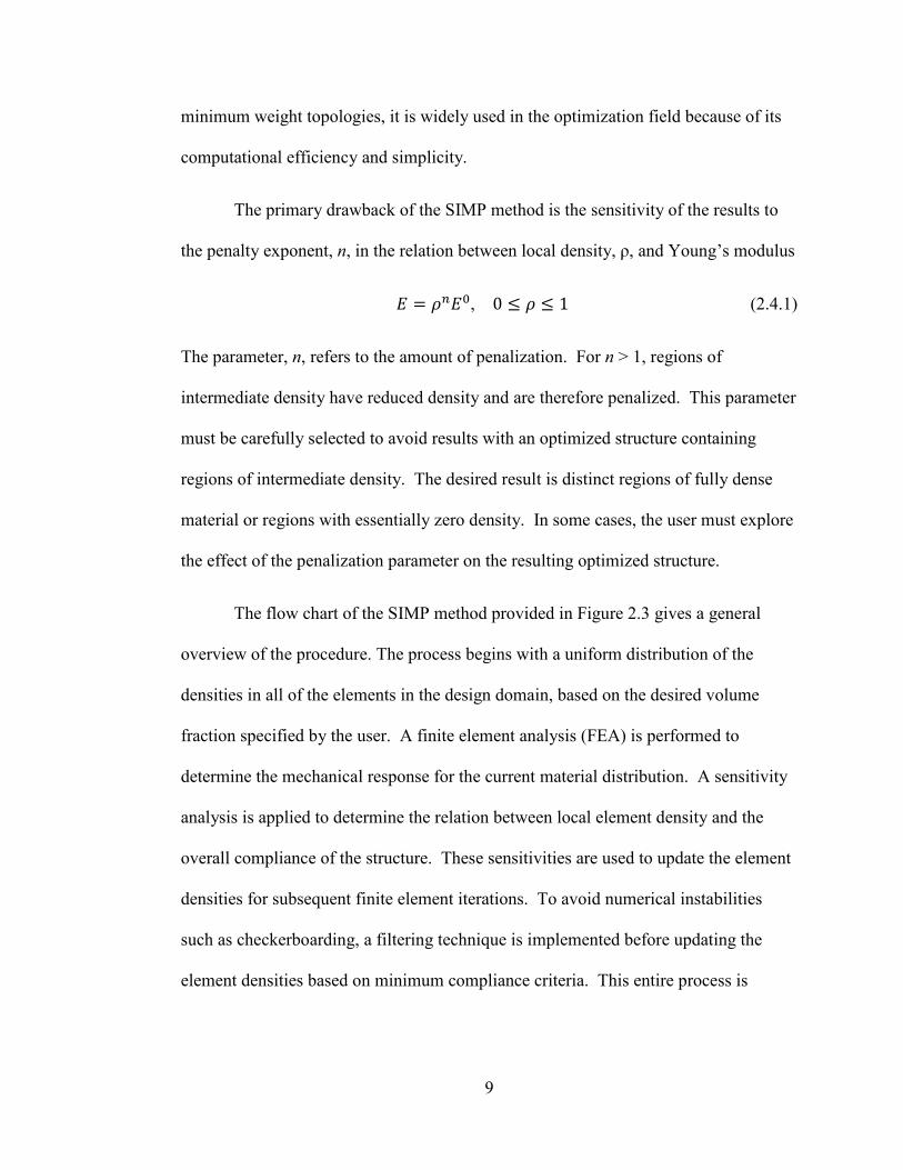
2.6 Numerical Problems

As with most numerical methods, there are deficiencies that may reduce the

effectiveness of the method. Topology optimization is no exception and these

deficiencies are well-documented in the literature. The most common types of

numerical problems in topology optimization are checkerboarding and mesh

dependence. Each of the sample problems discussed below are illustrated in Figure

2.5.

13

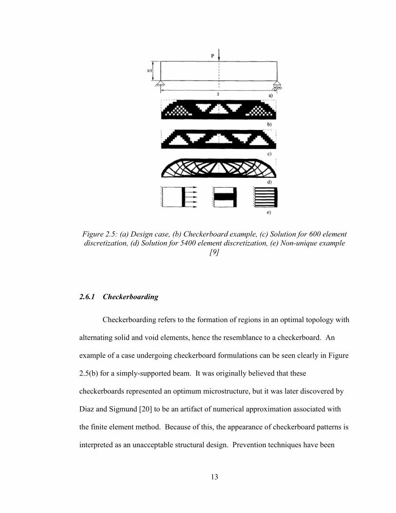
Figure 2.5: (a) Design case, (b) Checkerboard example, (c) Solution for 600 element discretization, (d) Solution for 5400 element discretization, (e) Non-unique example

[9]

2.6.1 Checkerboarding

Checkerboarding refers to the formation of regions in an optimal topology with

alternating solid and void elements, hence the resemblance to a checkerboard. An

example of a case undergoing checkerboard formulations can be seen clearly in Figure

2.5(b) for a simply-supported beam. It was originally believed that these

checkerboards represented an optimum microstructure, but it was later discovered by

Diaz and Sigmund [20] to be an artifact of numerical approximation associated with

the finite element method. Because of this, the appearance of checkerboard patterns is

interpreted as an unacceptable structural design. Prevention techniques have been

14

developed for the elimination of checkerboarding. These techniques include patches,

filtering, and higher-order finite elements.

The patch technique includes the formulation of an alternate finite element that

diminishes the appearance of checkerboards in most cases. The technique allows the

user to continue applying four-node quadrilateral elements, thus conserving CPU-time.

The result of patching introduces a “super-element” with a higher number of nodes

based on the density and displacement functions of the four surrounding elements. In

topology optimization however, the technique does not remove the checkerboard

effect entirely. Bendsøe [21] developed the patching process after he was inspired by

similar problems in Stokes flow.

In 1994, Sigmund [22] introduced the filtering technique, similar to image

filtering, where design sensitivities were altered and smoothed within each iteration.

The design sensitivity of each element became dependent on the average weight of the

element and its eight surrounding elements. In mathematical terms, the stiffness of a

point c depends on the density xc of all points in the surroundings, or neighborhood, of

c. The application of this filter reduces the topology complexity of an optimized

structure and ensures mesh-independency.

The use of higher-order finite elements for the displacement function can also

eliminate the issue of checkerboarding. For the SIMP method, it is suggested that

eight or nine-node quadrilateral elements be used to properly avoid checkerboards,

along with a combination of an element wise constant discretization of density [23].

However, the penalization power p needs to be small enough in order to obtain such

results. A paper published by Diaz and Sigmund [20] in 1995 suggested that p cannot

15

be any larger than 2.29. Unlike the patching technique though, CPU-time is

significantly increased under the higher-order finite element method because of the

introduction of additional degrees of freedom. For this reason, although higher-order

elements prevent checkerboarding, filtering techniques seem to be the preferred

method for suppressing checkerboarding.

2.6.2 Mesh Dependence

Due to inherent approximations associated with finite element based methods,

it is expected that the results of any finite element based topology optimization will be

mesh dependent. As the finite element mesh is refined, the structure increases in

detail and, in some cases, looks different all together. Figures 2.5(c) and 2.5(d)

demonstrate an example of this where a model with 600 elements is compared to a

5400 element model. The 5400 element discretization model exhibits a highly

detailed structure compared to the 600 element result.

Mesh-dependency results in a number of non-unique solutions for some cases

based on the mesh size and discretization applied. Figure 2.5(e) provides an example

of non-uniqueness where a structure undergoes uniaxial tension, but produces two

drastically different optimized structures. One has a single thick bar in the center and

the finer structure has several thin bars. Both models, however, are valid..

There are many techniques used for addressing mesh dependent problems such

as relaxation, perimeter control and global and local gradient constraint. The mesh-

independency filter has proven to be the most successful technique to this date for

three-dimensional cases. The mesh-independency filter is similar to the filtering

16

technique introduced for checkerboarding, except here the filtered design sensitivities

replace the real design sensitivities. Many users prefer the filtering technique

primarily because it requires no extra constraints to the optimization problem and little

to no extra CPU-time is needed.

2.7 Prescribed Material Redistribution

The Prescribed Material Redistribution (PMR) scheme was developed by

Taggart et al. [1-5] as an alternative method to optimizing topologies. In PMR, the

topology is identified through an iterative analysis where the relative material density

𝜌 (0 < 𝜌 ≤ 1) is varied. Initially, the material mass is distributed uniformly

throughout the desired design domain and results in a uniform, partially-dense

material. All of the nodes are assigned an initial relative density

𝜌0 = 𝑉𝑓𝑉𝐷

(2.7.1)

where Vf is the final structural volume and VD is the final domain volume. The initial

distribution and final cumulative distribution are defined, respectively, as

𝑓0(𝜌) = 𝛿(𝜌 − 𝜌0)

(2.7.2)

𝐹0(𝜌) = 𝐻(𝜌 − 𝜌0)

where f0 is the initial probability distribution function, F0 is the cumulative

distribution function, 𝛿 is the Dirac delta function and H is the Heaviside step

function.

17

The final relative material density distribution consists of regions that are fully

dense or nearly void, or 𝜌 = 1 and 𝜌 = 𝜌𝑚𝑖𝑛 (where 𝜌𝑚𝑖𝑛 ≪ 1) respectively. The

fully dense region is known as the optimal topology. The final probability distribution

function fF and final cumulative distribution function FF are defined as:

𝑓𝐹(𝜌) = (1 − 𝜌0)𝛿(𝜌 − 𝜌𝑚𝑖𝑛) + 𝜌0𝛿(𝜌 − 1)

(2.7.3)

𝐹𝐹(𝜌) = (1 − 𝜌0)𝐻(𝜌 − 𝜌𝑚𝑖𝑛) + 𝜌0𝐻(𝜌 − 1)

While the PMR method allows for various schemes for redistributing material,

the use of Beta probability distribution functions has been demonstrated to be effective

and efficient [1-5]. The gradual transition from the initial unimodal distribution to the

final distribution of fully-dense or void regions through the use of the Beta function β

in Eq. (2.7.4).

𝑓𝜌 = 𝛽(𝜌, 𝑟, 𝑠) = 𝜌𝑟−1(1−𝜌)𝑠−1Γ(r)Γ(s)Γ(r+s)

(2.7.4)

where Γ is the Gamma function and r and s are the adjustable parameters [4]. Then,

the corresponding cumulative distribution function is imposed through the use of the

incomplete Beta function βinc in Eq. (2.7.5).

𝐹𝜌 = 𝛽𝑖𝑛𝑐(𝜌, 𝑟, 𝑠) = 1𝛽(𝑟,𝑠)∫ (𝜌′)𝑟−1(1− 𝜌′)𝑠−1𝑑𝜌′𝜌

0 (2.7.5)

Typical families of Beta and incomplete Beta distribution functions for the case

𝜌0 = 0.3 are shown in Figures 2.6 and 2.7, respectively, where the evolution

parameter, t, is initially zero and is monotonically increased to a final value of one.

18

Appropriate functions r(t) and s(t) are specified [5] to provide a smooth transition

from the initial to the final material density distribution.

Figure 2.6: Transition from initial to final relative density distribution for the case 𝜌0 = 0.3 [4]

Figure 2.7: Transition from initial to final cumulative relative density distribution for the case 𝜌0 = 0.3 [4]

19

During each iteration, a detailed finite element analysis is performed. The

nodal strain energy densities are computed and then sorted; the nodes with highest

strain energy density are given highest relative density and the nodes with lowest

strain energy density are given lowest relative density. The desired relative density

distribution is then reached by assigning nodal densities based on sorted nodal strain

energy densities.

The PMR scheme is able to successfully identify topologies in an optimized

manner with high computational efficiency. Advantages include the enforcement of

constant material volume as it is redistributed to areas of high strain energy density. It

should be noted that the PMR scheme avoids the need for use of penalization factors

and filtering methods that, as described above, are required in other optimization

methods.

20

CHAPTER 3

FINITE ELEMENT ANALYSIS

This chapter discusses the Finite Element Method (FEM) and its

implementation in the three-dimensional PMR code. Element equations for three-

dimensional hexahedral elements are presented.

3.1 Three-Dimensional Elements

There are three basic groups of finite elements. These types include line

elements for one-dimensional analysis, planar elements for two-dimensional analysis,

and solid elements for three-dimensional analysis. Each group has their own sub-

category of elements that pertain differently to specific applications.

The introduction of three-dimensional solid elements provides a more realistic

approach to many applications in industry and research. Unlike two-dimensional

elements, three-dimensional analyses avoid the need for plane stress or plane strain

idealizations and can be used for general problems that are fully three-dimensional.

The use of three-dimensional elements has been made feasible by the advancements in

computer technology over the past few decades. There are a number of solid element

types available for three-dimensional analysis. These include the tetrahedron,

hexahedron and pentahedron elements. Each of the element types are illustrated in

Figure 3.1.

21

Figure 3.1: Three common element types in three-dimensional analysis [24]

The four-node tetrahedron, eight-node hexahedron, and six-node pentahedron are

among the basic forms of each element type because nodes are located only at the

corner points. The ten-node tetrahedron, twenty-node hexahedron, and fifteen-node

pentahedron provide improved accuracy by including nodes at the midpoint between

the corner point nodes. The additional nodes result in more degrees of freedom and

higher-order displacement interpolation within each element. Although higher-order

interpolation provides more realistic and accurate results, the run-time for each case is

substantially increased.

The four-node tetrahedron, or “tet”, is among the most popular and generalizes

with the planar triangular element formulation in two dimensions. Tetrahedral

elements provide the advantage of obtaining high quality meshes for complex

geometries and are commonly used in adaptive mesh refinement schemes [25].

However, four node tetrahedral elements are known to provide low accuracy and

hence, require very fine meshes for accurate results. The less common five-node

22

pentahedron element, also known as a triangular prism or wedge, is used mostly for

specialized applications such as the formation, propagation, and interrogation of

cracks, as well as the interlaminar delaminations in composites due to impact loadings

[25].

The element type selected for development in this thesis project is an eight-

node hexahedron, which is a three-dimensional generalization of the two-dimensional

quadrilateral element. Typically, hexahedral elements are taken to be rectangular

prisms, in which case they are also known as a brick or cube element. These elements

have eight nodes, six faces and twelve edges. Hexahedral elements are known to

provide improved accuracy for three-dimensional problems as compared to four-node

tetrahedral elements. An eight-node hexahedral element utilizes linear displacement

interpolation functions. In contrast, the four-node tetrahedral element which also uses

linear interpolation provides a state of constant strain within each element, resulting in

high discretization errors. Many researchers prefer the use of hexahedral elements in

non-linear problems because of severe locking problems associated with the use of

tetrahedral elements. Since the hexahedral element formulation was selected for

three-dimensional PMR method, the equations presented below are restricted to linear

eight-node, hexahedral elements.

3.2 Coordinate Systems

As is common in most finite element formulations, the hexahedral element

formulation involves consideration of two coordinate systems, a local coordinate

system in which the element has a cube shape where typically each coordinate varies

from -1 to +1 and a global coordinate system which represents the global coordinates

23

of the finite element mesh domain. Each coordinate system has its own node

numbering system.

3.2.1 Local Coordinate System

The local coordinate system, or normalized coordinate system, is mainly used

for numerical integration in computing the element stiffness matrix. The following

corner numbering rule is applied to ensure a positive Jacobian determinant at every

point in the element [25]. These rules are summarized as follows:

1. Choose one starting point, numbered node 1, and one initial face which

contains node 1.

2. Number the other corner points 2, 3 and 4 in counterclockwise fashion

(viewing from opposite face) on the initial face.

3. Number the opposite face the same way as the initial face, except 5, 6, 7

and 8 now.

The node numbering shown in Figure 3.2 below, followings these guidelines for the

corner numbering rule and will be used in the element formulation

24

Figure 3.2: Local coordinate system for a hexahedral element with appropriate node numbering

The coordinate axes shown are represented by the symbols s, t, and r with the origin of

the axis located in the center of the element. Note that the formulation below follows

the notation in Logan [26], with the exception that for simplicity in coding, r will be

used in place of Logan’s z’ coordinate. The coordinate locations of each of the eight

nodes are shown in Table 3.1. Note that the cube coordinates vary from -0.5 to +0.5

such that the length of each edge is unity and the centroid of the element is located at

the origin. Although this differs from the more commonly used variation from -1.0 to

+1.0, this difference is easily accounted for in the numerical integration of the element

stiffness matrix, as will be shown below.

25

Node (i) si ti ri 1 -0.5 -0.5 0.5 2 -0.5 -0.5 -0.5 3 -0.5 0.5 -0.5 4 -0.5 0.5 0.5 5 0.5 -0.5 0.5 6 0.5 -0.5 -0.5 7 0.5 0.5 -0.5 8 0.5 0.5 0.5

Table 3.1: Node numbering and coordinate locations for local hexahedral element

3.2.2 Global Coordinate System

The global coordinate system, or reference coordinate system, describes the

entire finite element domain being modeled. In general finite element formulations,

the element hexahedral shape in global coordinates can take on an arbitrary shape. For

this analysis, however, the element shape is taken to be a cube with unit length in all

three directions. Figure 3.3 below displays an illustration of three eight-node

hexahedral elements oriented along the x-axis and the node numbering scheme that

has been implemented.

26

Figure 3.3: Global coordinate system for multiple hexahedral elements with appropriate nodal numbering.

The global coordinate axes symbols are taken to be x, y, and z which are parallel to the

local coordinates s, t, and r, respectively. The node numbering scheme starts with

node 1 at the origin, followed by nodes 2, 3 etc. along the x-axis. Then, node

numbering continues at (x, y, z) = (0, 1, 0) and continues for all nodes with z = 0. This

numbering procedure continues at (x, y, z) = (0, 0, 1) and continues for all nodes with z

= 1. This procedure continues for the remaining nodes. From the user point of view,

specification of the number of nodes in the x, y and z-directions (nelx, nely and

nelz) fully defines the finite element mesh and the code automatically generates the

node numbering scheme described above.

3.3 Stresses and Strains

A three-dimensional stress state consists of six different stress components.

The normal stresses 𝜎𝑥, 𝜎𝑦 and 𝜎𝑧 are perpendicular to the element faces. In general,

these stresses change both the shape and volume of the material and are resisted by the

27

body’s elastic stiffnesses. In contrast, the shear stresses 𝜏𝑥𝑦, 𝜏𝑦𝑧 and 𝜏𝑧𝑥 are parallel

to the element faces. For isotropic materials, these stresses deform the material

without changing the volume and are resisted by the body’s shear modulus. For

isotropic materials, the material stiffness is fully characterized by two elastic

constants. In the formulation below, Young’s modulus and Poisson’s ratio are used to

characterize the material stiffness. In Figure 3.4, the stresses are displayed on a

typical three-dimensional element.

Figure 3.4: Three-dimensional element under a state of stress.

Similar to the stresses, there are six strain terms associated with a three-

dimensional strain state. These include the three normal strains 𝜀𝑥, 𝜀𝑦 and 𝜀𝑧 and

three engineering shear strains 𝛾𝑥𝑦, 𝛾𝑦𝑧 and 𝛾𝑧𝑥. The strains are proportional to

deformation gradients according to the following strain-displacement relationships

𝜀𝑥 = 𝜕𝑢𝜕𝑥

𝜀𝑦 = 𝜕𝑣𝜕𝑦

𝜀𝑧 = 𝜕𝑤𝜕𝑧

(3.3.1)

𝛾𝑥𝑦 = 𝜕𝑢𝜕𝑦

+ 𝜕𝑣𝜕𝑥

𝛾𝑦𝑧 = 𝜕𝑣𝜕𝑧

+ 𝜕𝑤𝜕𝑦

𝛾𝑧𝑥 = 𝜕𝑤𝜕𝑥

+ 𝜕𝑢𝜕𝑧

28

where u, v and w are the displacements in relation to the x, y and z coordinates,

respectively. The element strains and element stresses can also be specified in column

matrix form:

{𝜀} =

⎩⎪⎨

⎪⎧𝜖𝑥𝜀𝑦𝜀𝑧𝛾𝑥𝑦𝛾𝑦𝑧𝛾𝑧𝑥⎭

⎪⎬

⎪⎫

{𝜎} =

⎩⎪⎨

⎪⎧𝜎𝑥𝜎𝑦𝜎𝑧𝜏𝑥𝑦𝜏𝑦𝑧𝜏𝑧𝑥⎭

⎪⎬

⎪⎫

(3.3.2)

In matrix form, the stress-strain relationships can be written as

{𝜎} = [𝐶]{𝜀} (3.3.3)

where [𝐶] is the 6 x 6 elasticity matrix, also known as the constitutive matrix or

material property matrix. For an isotropic material, whose stiffness values are the

same in all directions, the elasticity matrix is defined in terms of Young’s modulus E

and Poisson’s ratio v in Eq. (3.3.4).

[𝐶] = 𝐸(1+ν)(1−2ν)

⎣⎢⎢⎢⎢⎢⎢⎡1 − ν ν ν 0 0 0ν 1 − ν ν 0 0 0ν ν 1 − ν 0 0 00 0 0 1−2ν

20 0

0 0 0 0 1−2ν2

0

0 0 0 0 0 1−2ν2 ⎦⎥⎥⎥⎥⎥⎥⎤

(3.3.4)

Young’s modulus represents the ratio of axial stress to axial strain in uniaxial

tension. Since a material under uniaxial tension must elongate in length, the value of

E is always greater than zero. Poisson’s ratio represents the negative of the ratio of

lateral strain to axial strain, and described as the lateral shrinkage in the material under

29

uniaxial tension. Although the theoretical range of values for v is from -1 to 0.5,

isotropic engineering materials typically exhibit a value between 0.25 and 0.35 [27].

3.4 Shape Functions

To accurately approximate the displacement field within the structure being

analyzed, proper shape functions must be derived and implemented. The shape

functions express the interpolation of the displacement function within the domain of

an element. For a linear displacement interpolation, the expression to define the shape

function is

𝑁𝑖 = �12

+ 𝑠𝑠𝑖� �12

+ 𝑡𝑡𝑖� �12

+ 𝑟𝑟𝑖� (3.4.1)

where s, t and r are the local coordinates and si, ti, and ri correspond to the coordinate

locations of the ith node, again in local coordinates. Hence, for the eight node

hexahedral element, the eight shape functions implemented are

𝑁1 = �12− 𝑠� �1

2− 𝑡� �1

2+ 𝑟� 𝑁2 = �1

2− 𝑠� �1

2− 𝑡� �1

2− 𝑟�

𝑁3 = �12− 𝑠� �1

2+ 𝑡� �1

2− 𝑟� 𝑁4 = �1

2− 𝑠� �1

2+ 𝑡� �1

2+ 𝑟�

(3.4.2) 𝑁5 = �1

2+ 𝑠� �1

2− 𝑡� �1

2+ 𝑟� 𝑁6 = �1

2+ 𝑠� �1

2± 𝑡� �1

2− 𝑟�

𝑁7 = �12

+ 𝑠� �12

+ 𝑡� �12− 𝑟� 𝑁8 = �1

2+ 𝑠� �1

2+ 𝑡� �1

2+ 𝑟�

Each shape function reduces to a value of one at the node i being referred to and zero

at all other nodes. As is typical of finite element interpolation functions, the sum of

the shape functions at any point in the element is a constant value of one.

30

3.5 Jacobian Matrix

The partial derivation of shape functions with respect to the global coordinates

x, y and z are required in the numerical integration for determining the element

stiffness matrix. The derivatives of the shape functions are given as chain rule

formulas, and shown in matrix form

⎣⎢⎢⎢⎡𝜕𝑁𝑖𝜕𝑥𝜕𝑁𝑖𝜕𝑦𝜕𝑁𝑖𝜕𝑧 ⎦⎥⎥⎥⎤

=

⎣⎢⎢⎢⎡𝜕𝑠𝜕𝑥

𝜕𝑡𝜕𝑥

𝜕𝑟𝜕𝑥

𝜕𝑠𝜕𝑦

𝜕𝑡𝜕𝑦

𝜕𝑟𝜕𝑦

𝜕𝑠𝜕𝑧

𝜕𝑡𝜕𝑧

𝜕𝑟𝜕𝑧⎦⎥⎥⎥⎤

⎣⎢⎢⎢⎡𝜕𝑁𝑖𝜕𝑠𝜕𝑁𝑖𝜕𝑡𝜕𝑁𝑖𝜕𝑟 ⎦⎥⎥⎥⎤ (3.5.1)

where the 3 x 3 matrix is the inverse Jacobian [𝐽]−1. The Jacobian is expressed as

[𝐽] = 𝜕(𝑥,𝑦,𝑧)𝜕(𝑠,𝑡,𝑟)

=

⎣⎢⎢⎢⎡𝜕𝑥𝜕𝑠

𝜕𝑦𝜕𝑠

𝜕𝑧𝜕𝑠

𝜕𝑥𝜕𝑡

𝜕𝑦𝜕𝑡

𝜕𝑧𝜕𝑡

𝜕𝑥𝜕𝑟

𝜕𝑦𝜕𝑟

𝜕𝑧𝜕𝑟⎦⎥⎥⎥⎤ (3.5.2)

and relates the local coordinates to the global coordinates. It can be regarded as a

scale factor that multiples ds dt dr to create the physical area increment dx dy dz.

When computing the determinant of the Jacobian matrix, the notation J is used.

3.6 Strain-Displacement Matrix

The displacement approximation in terms of shape functions is

{𝑢} = [𝑁]{𝑑} (3.6.1)

where {𝑑} refers to the nodal displacements in vector form. The relationship between

strains and displacements is needed in FEA to further compute the element stiffness

matrix and in computing the stress and strains from the nodal displacement results.

31

The strain-displacement matrix [𝐵] is introduced and equated as a function of s, t and

r. Derivation of [𝐵] as a function of the shape functions [𝑁] is shown in Eqs. (3.6.2)

and (3.6.3).

{𝜀} = [𝜕]{𝑢} = [𝜕][𝑁]{𝑑} = [𝐵]{𝑑} (3.6.2)

[𝐵] = [𝜕][𝑁] (3.6.3)

Using Eq. (3.6.3), the strain-displacement matrix [𝐵] can be expanded and shown as

the following 6 x 24 matrix:

[𝐵] =

⎣⎢⎢⎢⎢⎢⎢⎢⎢⎡𝜕𝑁1𝜕𝑠

0 0 𝜕𝑁2𝜕𝑠

0 0 𝜕𝑁3𝜕𝑠

0 0 𝜕𝑁4𝜕𝑠

0 0

0 𝜕𝑁1𝜕𝑡

0 0 𝜕𝑁2𝜕𝑡

0 0 𝜕𝑁3𝜕𝑡

0 0 𝜕𝑁4𝜕𝑡

0

0 0 𝜕𝑁1𝜕𝑟

0 0 𝜕𝑁2𝜕𝑟

0 0 𝜕𝑁3𝜕𝑟

0 0 𝜕𝑁4𝜕𝑟

𝜕𝑁1𝜕𝑡

𝜕𝑁1𝜕𝑠

0 𝜕𝑁2𝜕𝑡

𝜕𝑁2𝜕𝑠

0 𝜕𝑁3𝜕𝑡

𝜕𝑁3𝜕𝑠

0 𝜕𝑁4𝜕𝑡

𝜕𝑁4𝜕𝑠

0

0 𝜕𝑁1𝜕𝑟

𝜕𝑁1𝜕𝑡

0 𝜕𝑁2𝜕𝑟

𝜕𝑁2𝜕𝑡

0 𝜕𝑁3𝜕𝑟

𝜕𝑁3𝜕𝑡

0 𝜕𝑁4𝜕𝑟

𝜕𝑁4𝜕𝑡

𝜕𝑁1𝜕𝑠

0 𝜕𝑁1𝜕𝑠

𝜕𝑁2𝜕𝑟

0 𝜕𝑁2𝜕𝑠

𝜕𝑁3𝜕𝑟

0 𝜕𝑁3𝜕𝑠

𝜕𝑁4𝜕𝑟

0 𝜕𝑁4𝜕𝑠

�…

(3.6.4)

�

𝜕𝑁5𝜕𝑠

0 0 𝜕𝑁6𝜕𝑠

0 0 𝜕𝑁7𝜕𝑠

0 0 𝜕𝑁8𝜕𝑠

0 0

0 𝜕𝑁5𝜕𝑡

0 0 𝜕𝑁6𝜕𝑡

0 0 𝜕𝑁7𝜕𝑡

0 0 𝜕𝑁8𝜕𝑡

0

0 0 𝜕𝑁5𝜕𝑟

0 0 𝜕𝑁6𝜕𝑟

0 0 𝜕𝑁7𝜕𝑟

0 0 𝜕𝑁8𝜕𝑟

𝜕𝑁5𝜕𝑡

𝜕𝑁5𝜕𝑠

0 𝜕𝑁6𝜕𝑡

𝜕𝑁6𝜕𝑠

0 𝜕𝑁7𝜕𝑡

𝜕𝑁7𝜕𝑠

0 𝜕𝑁8𝜕𝑡

𝜕𝑁8𝜕𝑠

0

0 𝜕𝑁5𝜕𝑟

𝜕𝑁5𝜕𝑡

0 𝜕𝑁6𝜕𝑟

𝜕𝑁6𝜕𝑡

0 𝜕𝑁7𝜕𝑟

𝜕𝑁7𝜕𝑡

0 𝜕𝑁8𝜕𝑟

𝜕𝑁8𝜕𝑡

𝜕𝑁5𝜕𝑠

0 𝜕𝑁5𝜕𝑠

𝜕𝑁6𝜕𝑟

0 𝜕𝑁6𝜕𝑠

𝜕𝑁7𝜕𝑟

0 𝜕𝑁7𝜕𝑠

𝜕𝑁8𝜕𝑟

0 𝜕𝑁8𝜕𝑠 ⎦⎥⎥⎥⎥⎥⎥⎥⎥⎤

3.7 Stiffness Matrix

As a structure undergoes deformation through loading, the amount of

resistance to that deformation is determined by the global stiffness matrix, which

32

includes information related to both the geometry of the structure and the material

behavior. In the finite element formulation, the global stiffness matrix is found by

assembling the contribution of each of the element stiffness matrices.

3.7.1 Local Stiffness Matrix

The local stiffness matrix, or element stiffness matrix [𝑘] can best be

generalized in mathematical terms as

{𝑓} = [𝑘]{𝑑} (3.7.1)

where {𝑓} refers to the nodal forces acting on a single element. By itself, the element

stiffness matrix is singular, which means that it is non-invertible [27].

For an eight-node hexahedral element in three dimensions, the local stiffness

matrix expands to a 24 x 24 matrix according to

[𝑘] = ∫ ∫ ∫ [𝐵]𝑇[𝐶][𝐵]𝐽𝑑𝑠𝑑𝑡𝑑𝑟0.5−0.5

0.5−0.5

0.5−0.5 (3.7.2)

where the determinant of the Jacobian J is required to transform from the global

coordinates to the local coordinates. Each of the eight node points in an element have

three displacements, or degrees of freedom, in the s, t and r directions, resulting in a

total of 24 degrees of freedom in the element. The element equations relate these

degrees of freedom to the 24 nodal forces that act on the element.

3.7.2 Global Stiffness Matrix

The global stiffness matrix [𝐾] represents the entire structural domain and can

be written as

33

{𝐹} = [𝐾]{𝐷} (3.7.3)

where {𝐹} refers to the global forces and {𝐷} are the nodal displacements at the global

level. According to the Maxwell Reciprocal Theorem, all stiffness matrixes are

symmetric [𝐾] = [𝐾]𝑇. The global stiffness matrix is formed by expanding the

element equations to system size and assembling them to form the global equations.

These equations are modified to impose the displacement boundary conditions or

constraint conditions. The resulting system of linear equations are then solved to

determine the nodal displacements.

3.7.2 Stress and Strain Calculation

From the nodal displacements, Eqs. 3.3.4 and 3.6.2 are applied at the element

level to compute the strains and stresses, respectively, within the element. Typically

the stress and strain components are computed at the Gauss integration points,

extrapolated to the nodal positions and averaged with the result from adjacent

elements to provide an approximation of the nodal stresses and strain. The PMR

topology optimization algorithm also requires calculation of the nodal strain energy,

which can be computed directly from the nodal stress and strain results.

34

CHAPTER 4

THREE-DIMENSIONAL PMR CODE DEVELOPMENT

This chapter discuss the structure of the Matlab script that has been developed

to implement the three-dimensional PMR method. Following a short introduction of

Matlab, the key sections of the script are explained in detail, providing reference to

equations found in Chapter 3. The STL file generation is then introduced to explain

how these files are created for use in viewing the optimized 3-D structures and for

manufacture of components using 3-D printing technology.

4.1 Matlab Introduction

Matlab, short for “Matrix Laboratory”, is a powerful computer programming

language and interactive environment for code development. It is a commercial

software produced and provided by The Mathworks, Inc. Matlab is widely used by

scientists and engineers for matrix-based numerical computations and visualization. It

has includes a wide range of built in mathematical functions and can produce a wide

variety of graphical data visualizations. While Matlab was originally designed to

provide matrix-based computations, it has evolved over the years into a powerful

computational tool. Matlab is widely used as an instructional tool in universities for

introductory and advanced courses in computer programming, mathematics,

engineering and science. It is also widely used in industry and academia for research,

analysis, engineering design and development.

35

4.2 Overview of Matlab Script

The three-dimensional PMR Matlab script is divided into a number of

functions. These functions are explained in detail in the following subsections, along

with main terms translated and selected lines of code shown.

4.2.1 Parameter Initialization

Several parameters are to be specified by the user to define the particular

optimization problem. Typically, the user will write a short script that defines the

problem definition parameters. This script then calls the main function, pmr3D,

which performs the PMR topology optimization. Through a built-in post-processing

step, the optimized topology is converted to an STL file. STL is a standard graphic

file format in which the geometry is defined by triangular domains. It can be used for

viewing the 3-D geometry and manufacturing components using 3-D printing or other

additive manufacturing technologies.

The user defined parameters include specification of the design domain,

loading conditions, boundary conditions, number of PMR iterations (iter), and the

desired final volume fraction (volfrac). The domain is taken to be a rectangular

prism where the user specifies the number of elements nelx, nely and nely in the

x, y and z-directions, respectively. The finite element mesh that is used for the PMR

analysis consists of cube-shaped elements where the length, width and height of each

element is taken to be unity. Other parameters that the user must define are described

below.

36

For non-rectangular design domains, the user can define certain nodes to be

assigned a very low density, in effect creating a void region. Alternatively, the user

can define regions that are predefined to remain fully dense throughout the PMR

iterations. Regions that are not taken to be void regions or fully dense are those to

which the PMR algorithm is applied. Hence, these regions are considered to be the

design domain. Three different region types need to be defined by the user according

to values specified in Table 4.1.

Region Node Type Initial Nodal

Density numdesign 1 volfrac

numvoid 2 0.01 numdense 3 1

Table 4.1: Predefined regions with corresponding node type and node densities.

The final volume of the desired structure is specified through the volume

fraction parameter, volfrac, which represents the ratio of the final desired volume

to the volume of the region defined by the design nodes as specified by the number of

design nodes, numdesign. As described in Chapter 2, the PMR algorithm initially

assigns an intermediate density given by volfrac, to the design elements. At the

end of the procedure, the fraction of fully dense design elements is volfrac, and the

number of essentially void design elements is (1-volfrac). The predefined void

regions and fully dense regions are assigned nodal densities of 0.01 and 1,

respectively, the minimum and maximum density values. The value of 0.01 is used

since a density value of zero would lead to zero stiffness, which in return would result

in numerical difficulties for solving the finite element equations.

37

The PMR algorithm is implemented by imposing a specified density

distribution at each iteration through the use of the cumulative distribution functions

described in Chapter 2. As detailed in Chapter 2, families of Beta distribution

functions are used to impose a gradual transition from an initial state, where the design

nodes have a uniform initial density, volfrac, to a final state where the design

nodes are either nearly void or fully dense. The number of nodes that are fully dense

is determined such that the ratio of the volume of fully dense domain to the volume

associated with the design nodes is volfrac.

The loads and boundary conditions are specified by user defined array dbc

and forces. The dbc array is an Ndbc x 6 array in which columns 1 to 3 contain the

x, y and z coordinates of nodes for which displacement boundary conditions are to be

specified; columns 4 to 6 are either 0 or 1, with 0 specifying an unconstrained

displacement boundary condition and 1 specifying a constrained displacement

boundary condition. The number of rows in this array, Ndbc is the number of nodes for

which displacement boundaries are specified. All other nodes are taken to be

unconstrained. The array, forces, is an Nforce x 6 array where columns 1 to 3

contain the x, y and z coordinates of nodes for which force conditions are to be

specified and columns 4 to 6 are the x, y and z components of the force to be applied at

that node. The number of rows in this array, Nforce, is the number of nodes for which

forces are specified. All other nodes are taken to have zero external forces applied.

Users can also specify other model parameters relating to imposing symmetry

conditions. The array sym is a 1 x 3 array for which each value is 0 or 1

corresponding to the x, y or z coordinate axes. A value of 1 specifies that the plane

38

normal to the corresponding axis represents a symmetry plane. The sym array is used

in post-processing steps of STL file creation, where the parameters are used to

generate appropriate mirroring of the final topology. Note that for cases where

symmetry is desired, the user must define the appropriate displacement boundary

conditions using the array dbc, as described above. Finally, the user can impose

constraint relations, where a given displacement of a given node, called the slave

node, can be constrained to be equal to the corresponding displacement of another

node, called the master node. These relations are defined through the array,

constraint, where columns 1 to 3 are the x, y and z coordinates of the master node,

columns 4 to 6 are the x, y and z coordinates of the slave node, and columns 7 to 9 are

0 or 1, where the x, y or z component of the displacement of the slave node is forced to

equal the corresponding displacement of the master node if the value is 1.

The user parameters are sent to the pmr3d function using the command

pmr3d(nelx,nely,nelz,sym,volfrac,iter,node_type, (4.2.1) dbc,forces,constraint)

which performs iter iterations. For each iteration, the density distribution

prescribed by the PMR algorithm is imposed and a finite element analysis is then

performed to determine the resulting displacement, stress, strain and strain energy

fields. The 3-D finite element solver is contained in the function, FE, described

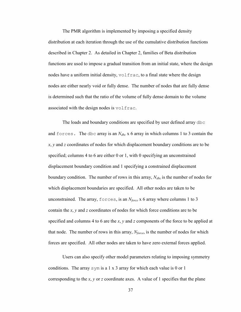
below. It should be noted that the pmr3d function uses the user defined arrays dbc,

forces and constraint to define the arrays fixeddofs, F and C that are used

as input to the function, FE.

39

4.2.2 Finite Element Function

The Finite Element (FE) function performs a finite element analysis for the

nodal density distribution corresponding to the current iteration. The call to the

function FE is shown in Eq. (4.2.2) and the terms are defined in Table 4.2.

function [Unew,Ut]=FE(nelx,nely,nelz,fixeddofs,F,C,x,xvec) (4.2.2)

Matlab Code Translation/Definition Unew Strain energy at each node Ut Total strain energy nelx Number of elements in x-direction nely Number of elements in y-direction nelz Number of elements in z-direction

fixeddofs Fixed degrees of freedom F Forces C Constraints x Density in 3-D matrix form

xvec Density values in vector form

Table 4.2: Matlab variable for the function FE

The function begins by initializing the key arrays as zeros or sparse. The

command zeros assigns values of 0 to all terms in a matrix or array. The command

sparse reduces memory storage by only storing non-zero values. The code

computes the element stiffness matrices (KE), the global stiffness matrix (K), the nodal

displacement vector (D), the stresses and strains at the Gauss points (strsg, strng),

the stresses and strains at the nodes (strsn, strnn), the strain energy at each node

(Unew) and the total strain energy (Ut). The three-dimensional finite element

equations developed in Chapter 3 are implemented in the function FE. In Table 4.3,

40

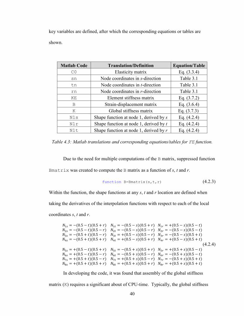
key variables are defined, after which the corresponding equations or tables are

shown.

Matlab Code Translation/Definition Equation/Table C0 Elasticity matrix Eq. (3.3.4) sn Node coordinates in s-direction Table 3.1 tn Node coordinates in t-direction Table 3.1 rn Node coordinates in r-direction Table 3.1 KE Element stiffness matrix Eq. (3.7.2) B Strain-displacement matrix Eq. (3.6.4) K Global stiffness matrix Eq. (3.7.3) N1s Shape function at node 1, derived by s Eq. (4.2.4) N1r Shape function at node 1, derived by t Eq. (4.2.4) N1t Shape function at node 1, derived by r Eq. (4.2.4)

Table 4.3: Matlab translations and corresponding equations/tables for FE function.

Due to the need for multiple computations of the B matrix, suppressed function

Bmatrix was created to compute the B matrix as a function of s, t and r.

function B=Bmatrix(s,t,r) (4.2.3)

Within the function, the shape functions at any s, t and r location are defined when

taking the derivatives of the interpolation functions with respect to each of the local

coordinates s, t and r.

𝑁1𝑠 = −(0.5 − 𝑡)(0.5 + 𝑟) 𝑁1𝑡 = −(0.5 − 𝑠)(0.5 + 𝑟) 𝑁1𝑟 = +(0.5 − 𝑠)(0.5 − 𝑡) 𝑁2𝑠 = −(0.5 − 𝑡)(0.5 − 𝑟) 𝑁2𝑡 = −(0.5 − 𝑠)(0.5 − 𝑟) 𝑁2𝑟 = −(0.5 − 𝑠)(0.5 − 𝑡) 𝑁3𝑠 = −(0.5 + 𝑡)(0.5 − 𝑟) 𝑁3𝑡 = +(0.5 − 𝑠)(0.5 − 𝑟) 𝑁3𝑟 = −(0.5 − 𝑠)(0.5 + 𝑡) 𝑁4𝑠 = −(0.5 + 𝑡)(0.5 + 𝑟) 𝑁4𝑡 = +(0.5 − 𝑠)(0.5 + 𝑟) 𝑁4𝑟 = +(0.5 − 𝑠)(0.5 + 𝑡)

(4.2.4) 𝑁5𝑠 = +(0.5 − 𝑡)(0.5 + 𝑟) 𝑁5𝑡 = −(0.5 + 𝑠)(0.5 + 𝑟) 𝑁5𝑟 = +(0.5 + 𝑠)(0.5 − 𝑡) 𝑁6𝑠 = +(0.5 − 𝑡)(0.5 − 𝑟) 𝑁6𝑡 = −(0.5 + 𝑠)(0.5 − 𝑟) 𝑁6𝑟 = −(0.5 + 𝑠)(0.5 − 𝑡) 𝑁7𝑠 = +(0.5 + 𝑡)(0.5 − 𝑟) 𝑁7𝑡 = +(0.5 + 𝑠)(0.5 − 𝑟) 𝑁7𝑟 = −(0.5 + 𝑠)(0.5 + 𝑡) 𝑁8𝑠 = +(0.5 + 𝑡)(0.5 + 𝑟) 𝑁8𝑡 = +(0.5 + 𝑠)(0.5 + 𝑟) 𝑁8𝑟 = +(0.5 + 𝑠)(0.5 + 𝑡)

In developing the code, it was found that assembly of the global stiffness

matrix (K) requires a significant about of CPU-time. Typically, the global stiffness

41

matrix assembly was more intensive than solving the global equations. In reviewing

the literature, the stiffness matrix assembly method introduced by Alejandro Ortiz-

Bernardin [28] proved to be very effective in reducing CPU-time required.

In solving the global equations, imposition of displacement boundary

conditions is simplified by defining which degrees of freedom are to be fixed and

which are free. Following the code by Sigmund [15], the arrays alldofs and

freedofs are defined as follows.

alldofs = 1:3*(nelx+1)*(nely+1)*(nelz+1); (4.2.5)

freedofs = setdiff(alldofs,fixeddofs);

All of the degrees of freedom (alldofs) are calculated in the first equation of Eq.

(4.2.5), which is based on three degrees of freedom for each node in the finite element

mesh. Then, in the second equation of Eq. (4.2.5), the free degrees of freedom,

freedofs, are determined by comparing alldofs to fixeddofs using the

Matlab command setdiff. Note that the array fixeddofs is provided as input to

the function FE. With these definitions, solution of the global equations can be

achieved with the command

D(freedofs,:) = K(freedofs,freedofs) \ F(freedofs,:); (4.2.6)

After solving the global equations, the nodal stresses, strains and strain energies are

computed using the finite element equations presented in Chapter 3. The array of

nodal strain energies, Unew, are returned to the main pmr3D function for use in

updating the nodal densities for the next iteration.

42

4.2.3 Symmetry Function

As mentioned above, the code provides the option to impose symmetry

conditions to reduce the amount of CPU-time and memory required for more complex

topology optimization problems. The combination of three-dimensional finite element

analysis, along with a large number of nodes required for complex problems can be

prohibitive in generating optimal designs. As a result, use of symmetry conditions

when appropriate is desired.

A structure undergoing symmetrical loadings and boundary conditions can be

analyzed within the PMR script. The symmetry displacement conditions are imposed

through careful specification of the displacement boundary conditions, dbc. In such

cases, the code creates appropriate mirroring of the optimal topology through the post-

processing creation of the STL geometry file. This is achieved using the function

stl_sym_gen which performs the geometry mirroring. The call to this function is

function [nx,ny,nz,node_def_new,el_def_new,dens_new]... (4.2.7)

=stl_sym_gen(nelx,nely,nelz,sym,node_def,el_def,dens)

In general, there are eight different cases of symmetry to consider under three-

dimensional analysis. The cases are acknowledged in the function as:

Case 1: no symmetry Case 2: x-symmetry Case 3: y-symmetry Case 4: z-symmetry Case 5: xy-symmetry Case 6: yz-symmetry Case 7: zx-symmetry Case 8: full (xyz) symmetry

43

To illustrate the procedure for mirroring the geometry, an excerpt of the

stl_sym_gen function for Case 5 with xy-symmetry is given below.

% Case 5 – XY Symmetry (1 1 0) if [ixsym iysym izsym]==[1 1 0] nx=2*nelx; ny=2*nely; nz=nelz; num=0; for nodez=1:nz+1 for nodey=1:ny+1 for nodex=1:nx+1 num=num+1; node_def_new(num,:)=[num,nodex-1,nodey-1,nodez-1]; end end end num=0; for elz=1:nz for ely=1:ny for elx=1:nx num=num+1; n1=elx+(ely-1)*(nx+1)+elz*(nx+1)*(ny+1); n2=n1-(nx+1)*(ny+1); n3=n2+(nx+1); n4=n1+(nx+1); n5=n1+1; n6=n2+1; n7=n3+1; n8=n4+1; el_def_new(num,:)=[n1,n2,n3,n4,n5,n6,n7,n8]; end end end % % Region 1 dens_new(1:nelx+1,1:nely+1,1:nelz+1)=d(nelx+1:-1:1,nely+1:-1:1,1:nelz+1); % Region 2 dens_new(1:nelx+1,nely+1:2*nely+1,1:nelz+1)=d(nelx+1:-1:1,1:nely+1,1:nelz+1); % Region 3 dens_new(nelx+1:2*nelx+1,1:nely+1,1:nelz+1)=d(1:nelx+1,nely+1:-1:1,1:nelz+1); % Region 4 dens_new(nelx+1:2*nelx+1,nely+1:2*nely+1,1:nelz+1)=d(1:nelx+1,1:nely+1,1:nelz+1); end

The specified plane of symmetry is determined by assigning a value to ixsym, iysym

and izsym, which impose symmetry along the x, y and z plane, respectively. A value

of 1 is assigned to denote the active symmetry while a value of 0 is inactive. The

dens_new term takes the optimized nodal density distribution and mirrors it about the

appropriate symmetry planes. The new density distribution, dens_new, is then used

in the STL generation function, described below.

44

4.3 STL File Generation

After the finite element results have been converged, the final bimodal material

distribution data is converted into contour surfaces of constant density. The contours

are then saved in STL format, which was originally implemented for use in the

stereolithography prototyping process but has also been identified as Standard

Tessellation Language. The STL file can be transmitted and viewed in standard CAD

viewer software. A free program called 3D Myriad Reader [29] was used throughout

the thesis project to view results of the case studies. The STL file can also be used as

direct input for producing prototypes with a rapid manufacturing 3-D printer or any

additive manufacturing process.

45

CHAPTER 5

ANALYSIS OF RESULTS

This chapter presents the results of several test cases that were developed to

validate the code and to demonstrate its capabilities. The first set of test cases

demonstrate the capability to model symmetry conditions by modeling the same

optimization problem with various symmetry conditions. The test case selected is a

simply-supported, centrally-loaded structure for which the minimum weight optimized

solution is well-known. The series of test cases focuses on optimizing the

microstructure of either porous or two-phase composite materials. Several different

cases for various multi-axial stress states are considered. Microstructures are then

developed through symmetry of unit cells and replication of unit cell results as a post-

processing operation.

5.1 Symmetry Conditions

To demonstrate the effectiveness of each case, the same example is run for the

first seven symmetry cases described below. This test case is based on a classical

Michell-arch structure. A.G.M. Michell [7] established the theoretical foundation of

minimum-weight structures in 1904 and showed that minimum weight structures

contain members subjected to uniaxial tension and compression, in a curved network

corresponding to directions of principal strain. The example considered in the

evaluation of the PMR scheme is for the case of a center load applied mid-span

between two pinned supports. The PMR design domain is extended beyond the

support points such that the optimized structure lies fully within the specified domain.

46

The theoretical optimized Michell-arch structure for this loading (see Figure 5.1)

consists of radial members to the central load point on an arch structure to the support

points.

Figure 5.1: Theoretical optimal Michell-arch structure.

Seven test cases were developed using various combinations of symmetry

planes as listed in Table 5.1. It can be seen that for all cases, the PMR method gives a

reasonable representation of the theoretical optimal solution. The total CPU-time for

each case has been recorded in minutes and the main parameters are specified in Table

5.1 below.

Case volfrac nelx nely nelz Total DOF's

iter CPU (min)

Efficiency (%)

1 0.16 48 42 10 60480 100 76.4 0 2 0.16 24 42 10 30240 100 32.6 57 3 0.16 48 5 42 30240 100 30.2 60 4 0.16 48 42 5 30240 100 29.9 61 5 0.16 24 5 42 15120 100 15.2 80 6 0.16 24 42 5 15120 100 15 80

6B 0.06 40 70 8 67200 100 86.2 N/A 7 0.16 42 5 24 15120 100 14.6 81

Table 5.1: Total CPU-time results for similar Michell-arch example using first seven symmetry cases

47

The efficiency column refers to the percentage of time eliminated in comparison with

Case 1 exhibiting no symmetry. The data reveals that the simplest form of symmetry

(x, y, or z) results in a total time reduced to more than half; with other symmetries

reduced to more than three-quarters. It is important to note that these times will vary

depending on the computer being used; the efficiency values, however, should remain

approximately the same. For Case 6B, the number of elements were increased, which,

as expected, resulted in an increased CPU-time. In this case, a smaller volume

fraction, 0.06, was used, resulting in the structure shown in Figure 5.2. The predicted

topology is consistent with the theoretical Michell-arch structure. Structures from the

remaining seven cases are shown in Appendix A.

Figure 5.2: Michell-arch result using xy-symmetry for Case 6B

The Michell-arch case is not appropriate for validating the full symmetry

feature due to its geometrical orientation and loading conditions. Therefore, a separate

48

unique case was considered in order to validate the effectiveness of Case 8. The

loading conditions for this case are shown in Figure 5.3, where the outlined red region

represents the section being mirrored amongst the other seven regions.

Figure 5.3: Initial conditions for Case 8 with full symmetry

The example was run for three different conditions as shown in Table 5.2. In

Case 8A, no symmetry was used with twenty elements in each of the three directions.

For Case 8B and 8C however, full symmetry was used with ten elements and twenty

elements, respectively, in each of the three directions. Results for Cases, 8A, 8B and

8C are displayed in Figure 5.4 below. It can be seen that through the use of symmetry,

e.g. Case 8A vs. 8B, dramatic reductions in CPU-time can be achieved. Alternatively,

use of symmetry can be used to provide more precise results, e.g. Case 8A vs. 8C,

with comparable CPU-times.

Case volfrac nelx nely nelz Total DOF's

iter CPU (min)

8A 0.1 20 20 20 24000 100 32.4 8B 0.1 10 10 10 3000 100 2.9 8C 0.1 20 20 20 24000 100 34.6

Table 5.2: Total CPU-time results for similar unique example using no symmetry (Case 8A) and full symmetry (Case 8B and 8C)

49

Figure 5.4: Full symmetry test cases results: Case 8A (top), Case 8B (middle) and 8C (bottom)

50

5.2 Microstructures

This section will focus on developing microstructures using one-eighth unit

cell models, which are mirrored to the other seven regions using symmetry conditions.

In Figure 5.5 below, the initial region selected for the unit model is designated by the

dashed red outline.

Figure 5.5: Outline of unit cell model region

In order to accurately develop a final microstructure, proper constraints must be

applied to the faces of the unit cell. On the interior faces, displacements normal to the

plane are zero and on the exterior faces, displacements normal to the plane are

uniform. In Figure 5.6, these constraints are shown with the interior faces color-coded

based on the applied constraint. The green face applies zero displacement in the x-

direction, the red face for the y-direction, and the blue face for the z-direction.

51

Figure 5.6: Unit cell model with constraints shown

5.2.1 Porous Microstructures

A number of cases were considered for various stress states. Each case utilized

a volume fraction of 0.2 and the number of iterations was taken to be 100. To model a

porous material, the fully dense domain was assigned a Young’s modulus of 1.0 and

the void region was assigned a modulus of 0.01. As specified in Table 5.3, various

multi-axial stresses were then applied. Table 5.3 shows the stress states for each case

and the corresponding microstructures in Figure 5.7.

Figure 5.7( ) σx σy σz a 1 0 0 b 1 1 0 c 1 -1 -1 d 1 0.5 0.5 e 1 0.75 0.75 f 1 1.25 1.25 g 1 1.5 1.5 h 1 0.5 1

Table 5.3: Stress values for each porous microstructure figure

52

(a)

(b)

(c)

(d)

53

(e)

(f)

(g)

(h)

Figure 5.7: Microstructures made of porous materials; (a) through (h) cases correspond to conditions in Table 5.3

54

For each case, the image on the left refers to a quarter of the material’s unit cell.

Symmetry conditions are applied to create a single unit cell result in order to conserve

CPU-time. The full model results (right hand side of Figure 5.7) represent a 6 x 6 x 6

mirroring , or replication, of the unit cell results. The array was made possible by a

Matlab script called stl_gen_3d_array function.

The most consistent formation within each microstructure are the plates of

material. The plates are strategically placed depending on the value and location of

the two equal stress states. If the equal stress values are larger than the third stress, a

solid plate of unknown thickness is formed on the plane of where those stresses are.

The figures exemplifying this scenario are 5.7(b), 5.7(f), 5.7(g) and 5.7(h). If the

equal stress values are not zero and lower than the third stress, a solid plate is not

formed and instead the material is distributed mostly on the other two planes. Figures

5.7(d) and 5.7(e) match this scenario and contain many regions of hollow or void

material.

For cases with a dominant load direction, fibrous microstructures provide the

optimal geometry. Figure 5.7(g) portrays exactly that with hollow fibers in the x-

plane. A slightly different scenario involves uni-axial stress, where two or three stress

states are zero. There lies uni-axial stress in the x-direction of Figure 5.7(a), which

explains the single fibers in each array along with no other supporting material.

5.2.2 Composite Microstructures

Similar to the cases discussed above for porous microstructures, this section

will focus on composite microstructures and slightly different conditions. The stress

55

states, number of iterations and volume fraction all remain the same for each case,

however, the domain consists of a two phase composite in which the stiffer phase has

a Young’s Modulus of unity and the lower stiffness phase has aYoung’s Modulus of

0.5. . Table 5.4 shows the applied stress statescorresponding to the microstructures in

Figure 5.8.

Figure 5.8( ) σx σy σz a 1 0 0 b 1 1 0 c 1 -1 -1 d 1 0.5 0.5 e 1 0.75 0.75 f 1 1.25 1.25 g 1 1.5 1.5

Table 5.4: Stress values for each composite microstructure figure

(a)

56

(b)

(c)

(d)

(e)

57

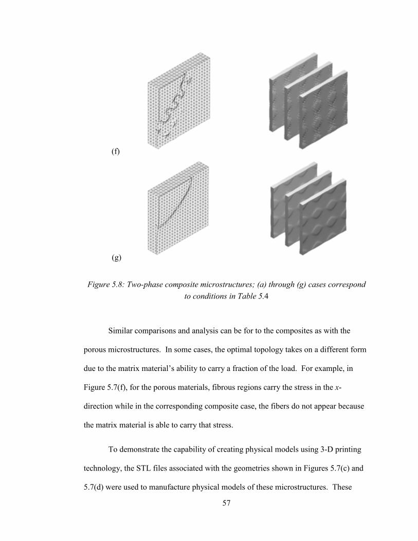
(f)

(g)

Figure 5.8: Two-phase composite microstructures; (a) through (g) cases correspond to conditions in Table 5.4

Similar comparisons and analysis can be for to the composites as with the

porous microstructures. In some cases, the optimal topology takes on a different form

due to the matrix material’s ability to carry a fraction of the load. For example, in

Figure 5.7(f), for the porous materials, fibrous regions carry the stress in the x-

direction while in the corresponding composite case, the fibers do not appear because

the matrix material is able to carry that stress.

To demonstrate the capability of creating physical models using 3-D printing

technology, the STL files associated with the geometries shown in Figures 5.7(c) and

5.7(d) were used to manufacture physical models of these microstructures. These

58

models were manufactured on a Dimension Model SST 3-D Printer. Photographs of

these models are shown in Figure 5.9 and 5.10.

Figure 5.9: 3-D printed physical model of case shown in Figure 5.7(c)

Figure 5.10: 3-D printed physical model of case shown in Figure 5.7(d)

59

CHAPTER 6

CONCLUSIONS AND FUTURE WORK

Due to economic and environmental reasons, the interest in topology

optimization and minimum weight structures has increased significantly in recent

years. The PMR scheme as implemented in the Matlab script provides an effective

tool for the identification of optimized structures; as well as graphically representing

them in an external CAD program or for manufacturing with an additive

manufacturing process.

The Matlab script developed in this research provides a self-contained code in

which the user can easily define a general 3-D topology optimization problem and the

code output includes an STL model file that represents the optimized topology.

Several test cases are presented which confirm the ability of the code to successfully

identify the known optimal topology for a particular structure. Future work could

include more exhaustive validations of the code for other load configurations. The

second set of test cases involved the determination of optimal microstructures for

porous and two-phase composite materials. While the results obtained appear to be

qualitatively reasonable, future work should develop more rigorous validation cases

for which the optimal microstructure can be established either analytically or through

some other optimization procedure. Such analyses are required to confirm whether the

PMR scheme can accurately identify optimal microstructures for porous or composite

materials.

60

This work included significant effort to optimize the computational efficiency

of the code, particularly through imposition of symmetry conditions and the

implementation of an efficient element assembly method. Although attempts were

made to improve the efficiency of the Matlab solver in solving the global equations,

the default solver as provided by the Matlab “backslash” equation solver proved to be

the most efficient. Future work, however, should include further efforts to improve

computational efficiency, perhaps through the use of iterative equations solvers and/or

parallelization of parts of the code for efficient use of computers with parallel

processing capabilities.

Finally, after thorough validation of the PMR code for the optimization of

multi-phase composites, this method has the potential to provide an excellent tool for

exploring methods for optimizing the local microstructure of structures. The

microstructure of traditional composites is constrained by available manufacturing

methods and the resulting configuration of reinforcing and matrix phases. With the

advent of additive manufacturing methods where multiple phases can be deposited in

any imaginable configuration, opportunities exist to locally tailor the microstructure

based on the local stress state. Design tools such as the PMR optimization method,

coupled with emerging manufacturing methods, could lead to a new generation of

lightweight and strong materials.

61

APPENDIX A

SYMMETRY TEST CASES

Figure A.1: Michell-Arch results using no symmetry for Case 1

Figure A.2: Michell-Arch results using x-symmetry for Case 2

Figure A.3: Michell-Arch results using y-symmetry for Case 3

62

Figure A.4: Michell-Arch results using z-symmetry for Case 4

Figure A.5: Michell-Arch results using xy-symmetry for Case 5

Figure A.6: Michell-Arch results using zx-symmetry for Case 6

Figure A.7: Michell-Arch results using yz-symmetry for Case 7

63

APPENDIX B

MATLAB SCRIPT FOR SYMMETRY CASES

The Matlab script for the Michell-arch symmetry cases is given below. Upon

running the script, the user will be asked to specify which cases to run. By entering 1,

all of the cases will run sequentially. If a single case is desired, the user may enter the

case number manually when asked.

Within the loop of each case, the parameters are initialized and defined

appropriately depending on the geometrical orientation. These parameters include

nelx, nely, nelz, node_type, volfrac, iter, dbc, forces, sym, and

constraint. After the loop is completed, the PMR_3D main script is called and the

results and appropriate symmetry conditions are imposed to generate an STL file for

viewing in an outside program such as 3D Myriad Reader.

% symmetry cases % clc; clear all; close all; format compact % % user input to select cases iloop=input('Enter 1 to run all cases: '); if iloop ~=1 cases=['Case 1 - no symmetry '; 'Case 2 - x symmetry '; 'Case 3 - y symmetry '; 'Case 4 - z symmetry '; 'Case 5 - xy symmetry '; 'Case 6 - xz symmetry '; 'Case 7 - yz symmetry '; 'Case 8 (8A) - no symmetry '; 'Case 9 (8B) - xyz symmetry '; 'Case 10(8C) - xyz symmetry (fine)']; disp(cases) case_num=input('Enter case number: '); end clc if iloop==1 range=1:10; else range=case_num:case_num; end max_iter=100; % run selected cases

64

for icase=range % clear nelx nely nelz sym volfrac iter node_type dbc forces if icase==1 disp('Case 1 - no symmetry') % define model parameters nelx=48; nely=42; nelz=10; node_type(1:(nelx+1)*(nely+1)*(nelz+1))=1; volfrac=0.16; iter=max_iter; % define loads and boundary conditions dbc=[ .9375*nelx .5*nely .5*nelz 1 1 1; .0625*nelx .5*nely .5*nelz 1 1 1 0 0 0 0 0 1]; forces=[.5*nelx .5*nely .5*nelz 0 -1 0]; sym=[0 0 0]; % call PMR constraint=[]; PMR_3D(nelx,nely,nelz,sym,volfrac,iter,node_type,dbc,forces,constraint); % rename stl file movefile('model.stl','no_sym.stl') % %------------------------------------------------------------------ % elseif icase==2 disp('Case 2 - x symmetry') % define model parameters nelx=24; nely=42; nelz=10; node_type(1:(nelx+1)*(nely+1)*(nelz+1))=1; volfrac=0.16; iter=max_iter; sym=[1 0 0]; % define loads and boundary conditions dbc=zeros((nelx+1)*(nely+1)*(nelz+1),6); irow=0; for x=0:nelx for y=0:nely for z=0:nelz irow=irow+1; % Define dbc if x==.875*nelx && y==nely/2 && z==nelz/2 dbc(irow,:)=[ x y z 1 1 1]; elseif x==0 && y==0 && z==0 dbc(irow,:)=[ x y z 0 0 1]; elseif x==0 dbc(irow,:)=[ x y z 1 0 0]; end end end end dbc(all(dbc==0,2),:)=[]; forces=[0 nely/2 nelz/2 0 -10 0]; % call PMR constraint=[]; PMR_3D(nelx,nely,nelz,sym,volfrac,iter,node_type,dbc,forces,constraint); % rename stl file movefile('model.stl','x_sym.stl')

65

% %------------------------------------------------------------------ % elseif icase==3 disp('Case 3 - y symmetry') % define model parameters nelx=48; nely=5; nelz=42; node_type(1:(nelx+1)*(nely+1)*(nelz+1))=1; volfrac=0.16; iter=max_iter; sym=[0 1 0]; % define loads and boundary conditions dbc=zeros((nelx+1)*(nely+1)*(nelz+1),6); irow=0; for x=0:nelx for y=0:nely for z=0:nelz irow=irow+1; % Define dbc if x==.9375*nelx && y==0 && z==nelz/2 dbc(irow,:)=[ x y z 1 1 1]; elseif x==.0625*nelx && y==0 && z==nelz/2 dbc(irow,:)=[ x y z 1 1 1]; elseif y==0 dbc(irow,:)=[ x y z 0 1 0]; end end end end dbc(all(dbc==0,2),:)=[]; forces=[nelx/2 0 nelz/2 0 0 10]; % call PMR constraint=[]; PMR_3D(nelx,nely,nelz,sym,volfrac,iter,node_type,dbc,forces,constraint); % rename stl file movefile('model.stl','y_sym.stl') % %------------------------------------------------------------------ % elseif icase==4 disp('Case 4 - z symmetry') % define model parameters nelx=48; nely=42; nelz=5; node_type(1:(nelx+1)*(nely+1)*(nelz+1))=1; volfrac=0.16; iter=max_iter; sym=[0 0 1]; % define loads and boundary conditions dbc=zeros((nelx+1)*(nely+1)*(nelz+1),6); irow=0; for x=0:nelx for y=0:nely for z=0:nelz irow=irow+1; % Define dbc if x==.9375*nelx && y==nely/2 && z==0 dbc(irow,:)=[ x y z 1 1 1]; elseif x==.0625*nelx && y==nely/2 && z==0

66

dbc(irow,:)=[ x y z 1 1 1]; elseif z==0 dbc(irow,:)=[ x y z 0 0 1]; end end end end dbc(all(dbc==0,2),:)=[]; forces=[nelx/2 nely/2 0 0 -10 0]; % call PMR constraint=[]; PMR_3D(nelx,nely,nelz,sym,volfrac,iter,node_type,dbc,forces,constraint); % rename stl file movefile('model.stl','z_sym.stl') % %------------------------------------------------------------------ % elseif icase==5 disp('Case 5 - xy symmetry') % define model parameters nelx=24; nely=5; nelz=42; node_type(1:(nelx+1)*(nely+1)*(nelz+1))=1; volfrac=0.16; iter=max_iter; sym=[1 1 0]; % define loads and boundary conditions dbc=zeros((nelx+1)*(nely+1)*(nelz+1),6); irow=0; for x=0:nelx for y=0:nely for z=0:nelz irow=irow+1; % Define dbc if x==.875*nelx && y==0 && z==nelz/2 dbc(irow,:)=[ x y z 1 1 1]; elseif x==0 && y==0 dbc(irow,:)=[ x y z 1 1 0]; elseif x==0 dbc(irow,:)=[ x y z 1 0 0]; elseif y==0 dbc(irow,:)=[ x y z 0 1 0]; end end end end dbc(all(dbc==0,2),:)=[]; forces=[0 0 nelz/2 0 0 10]; % call PMR constraint=[]; PMR_3D(nelx,nely,nelz,sym,volfrac,iter,node_type,dbc,forces,constraint); % rename stl file movefile('model.stl','xy_sym.stl') % %------------------------------------------------------------------ % elseif icase==6 disp('Case 6 - xz symmetry') % define model parameters nelx=24;

67

nely=42; nelz=5; node_type(1:(nelx+1)*(nely+1)*(nelz+1))=1; volfrac=0.16; iter=max_iter; sym=[1 0 1]; % define loads and boundary conditions dbc=zeros((nelx+1)*(nely+1)*(nelz+1),6); irow=0; for x=0:nelx for y=0:nely for z=0:nelz irow=irow+1; % Define dbc if x==.875*nelx && y==nely/2 && z==0 dbc(irow,:)=[ x y z 1 1 1]; elseif x==0 dbc(irow,:)=[ x y z 1 0 0]; elseif z==0 dbc(irow,:)=[ x y z 0 0 1]; end end end end dbc(all(dbc==0,2),:)=[]; forces=[0 nely/2 0 0 -10 0]; % call PMR constraint=[]; PMR_3D(nelx,nely,nelz,sym,volfrac,iter,node_type,dbc,forces,constraint); % rename stl file movefile('model.stl','xz_sym.stl') % %------------------------------------------------------------------ % elseif icase==7 disp('Case 7 - yz symmetry') % define model parameters nelx=42; nely=5; nelz=24; % node_type(1:(nelx+1)*(nely+1)*(nelz+1))=1; volfrac=0.16; iter=max_iter; sym=[0 1 1]; % define loads and boundary conditions dbc=zeros((nelx+1)*(nely+1)*(nelz+1),6); irow=0; for x=0:nelx for y=0:nely for z=0:nelz irow=irow+1; % Define dbc if x==nelx/2 && y==0 && z==.875*nelz dbc(irow,:)=[ x y z 1 1 1]; elseif y==0 && z==0 dbc(irow,:)=[ x y z 0 1 1]; elseif y==0 dbc(irow,:)=[ x y z 0 1 0]; elseif z==0 dbc(irow,:)=[ x y z 0 0 1]; end

68

end end end dbc(all(dbc==0,2),:)=[]; forces=[nelx/2 0 0 10 0 0]; % call PMR constraint=[]; PMR_3D(nelx,nely,nelz,sym,volfrac,iter,node_type,dbc,forces,constraint); % rename stl file movefile('model.stl','yz_sym.stl') % %------------------------------------------------------------------ % elseif icase==8 disp('Case 8A - no symmetry') % define model parameters nelx=20; nely=nelx; nelz=nelx; % node_type(1:(nelx+1)*(nely+1)*(nelz+1))=1; volfrac=0.1; iter=max_iter; sym=[0 0 0]; % define loads and boundary conditions dbc(1,:)=[ 3 3 3 1 1 1]; dbc(2,:)=[ 17 3 3 0 1 1]; dbc(3,:)=[ 3 17 3 0 0 1]; forces=[ 3 3 3 -10 -10 -10; 3 3 17 -10 -10 10; 3 17 3 -10 10 -10; 3 17 17 -10 10 10; 17 3 3 10 -10 -10; 17 3 17 10 -10 10; 17 17 3 10 10 -10; 17 17 17 10 10 10]; % call PMR constraint=[]; PMR_3D(nelx,nely,nelz,sym,volfrac,iter,node_type,dbc,forces,constraint); % rename stl file movefile('model.stl','8A_no_sym.stl') % %------------------------------------------------------------------ % elseif icase==9 disp('Case 8B - xyz symmetry') % define model parameters nelx=10; nely=nelx; nelz=nelx; % node_type(1:(nelx+1)*(nely+1)*(nelz+1))=1; volfrac=0.1; iter=max_iter; sym=[1 1 1]; % define loads and boundary conditions dbc=zeros((nelx+1)*(nely+1)*(nelz+1),6); irow=0; for x=0:nelx for y=0:nely for z=0:nelz

69

irow=irow+1; % Define dbc if x==0 || y==0 || z==0 dbc(irow,:)=[x y z ~x ~y ~z]; end end end end dbc(all(dbc==0,2),:)=[]; forces=[7 7 7 10 10 10]; % call PMR constraint=[]; PMR_3D(nelx,nely,nelz,sym,volfrac,iter,node_type,dbc,forces,constraint); % rename stl file movefile('model.stl','8B_xyz_sym.stl') % %------------------------------------------------------------------ % elseif icase==10 disp('Case 8C - xyz symmetry (fine mesh)') % define model parameters nelx=20; nely=nelx; nelz=nelx; % node_type(1:(nelx+1)*(nely+1)*(nelz+1))=1; volfrac=0.1; iter=max_iter; sym=[1 1 1]; % define loads and boundary conditions dbc=zeros((nelx+1)*(nely+1)*(nelz+1),6); irow=0; for x=0:nelx for y=0:nely for z=0:nelz irow=irow+1; % Define dbc if x==0 || y==0 || z==0 dbc(irow,:)=[x y z ~x ~y ~z]; end end end end dbc(all(dbc==0,2),:)=[]; forces=[14 14 14 10 10 10]; % call PMR constraint=[]; PMR_3D(nelx,nely,nelz,sym,volfrac,iter,node_type,dbc,forces,constraint); % rename stl file movefile('model.stl','8C_xyz_sym.stl') end % end

70

BIBLIOGRAPHY

[1] Taggart, D. G., Dewhurst, P., Dobrot, L., and Gill, D., “Development of a Beta Function Based Topology Optimization Procedure,” 2008 Abaqus Users Conference, Newport, RI, May 2008.

[2] Taggart, D. G. and Dewhurst, P., “A Novel Numerical Topology Optimization Method,” 8th World Congress on Computational Mechanics and 5th European Congress on Computational Methods in Applied Sciences and Engineering, July 2008.

[3] Taggart, D. G., Jahns, D., Nair, A. and Dewhurst, P., “Application of the PMR Topology Optimization Scheme to Dual Material Structures,” ASME 2010 International Mechanical Engineering Congress and Exposition, Vancouver, Canada, November 2010.

[4] Taggart, D. G. and Dewhurst, P., “Development and Validation of a Numerical Topology Optimization Scheme for Two and Three Dimensional Structures,” Advances in Engineering Software, 41, 910-915, 2010.

[5] Taggart, D. G., Dewhurst, P. and Nair, A. “System and Methods for Finite Element Based Topology Optimization”, US. Patent 8.335.668, 2012.

[6] Wilde, D.J. and Beightler, C.S., Foundations of Optimization, Prentice-Hall, Inc., 1967.

[7] Michell, A.G.M. LVIII. “The Limits of Economy of Material in Frame-Structures,” The London, Edinburgh, and Dublin Philosophical Magazine and Journal of Science, 8(47):589-597, 1904.

[8] Schmit, L.A., “Structural Design by Systematic Synthesis,” Second Conference on Electronic Computation, ASCE, Pittsburg, 105-132, 1960.

[9] Bendsøe, M.P. and Sigmund, O., “Topology Optimization,” Springer-Verlag, 2004.

[10] Sant'Anna, Hervandil M., and Jun S.O. Fonseca. “Topology Optimization of Continuum Two-Dimensional Structures under Compliance and Stress Constraints,” Tech. Vol. 21. Brazil: n.p., 2002. Print.

[11] Bendsøe, M.P., “Optimal shape design as a material distribution problem,” Structural Optimization 1. 193-202. 1989.

71

[12] Rozvany, G.I.N., Zhou, M. and Birker, T., “Generalized shape optimization without homogenization,” Structural Optimization 4. 250-254. 1992.

[13] Browne, Philip A. "Topology Optimization of Linear Elastic Structures." Thesis. University of Bath, 2013. Print.

[14] Aremu, A., I. Ashcroft, R. Hague, R. Wildman, and C. Tuck. Suitability of SIMP and BESO Topology Optimization Algorithms for Additive Manufacturing. Tech. Loughborough : n.p., 2010. Print.

[15] Sigmund, O., “A 99 line topology optimization code written in Matlab,” Structural and Multidisciplinary Optimization, Volume 21 Issue 2, 120-127, 2001.

[16] Xie, Y.M. and Steven G.P., Evolutionary Structural Optimization, Springer-Verlag, Berlin, 1997.

[17] Xie, Mike. "Evolutionary Structural Optimization." Innovative Structures and Materials. RMIT, n.d. Web. 1 Mar. 2014. <http://www.rmit.edu.au/browse/Research%2FInstitutes,%20Centres%20and%20Groups%2FCentres%2FInnovative%20Structures%20and%20Materials%2FProjects%2FEvolutionary%20Structural%20Optimisation/>

[18] O.M. Querin, G.P. Steven, Y.M. Xie, Evolutionary structural optimization (ESO) using a bidirectional algorithm, Engineering Computations, Vol. 15 Iss: 8, pp.1031 - 1048. 1998.

[19] Boer, Edward D. Topology and Shape Optimization for Non-Linear Problems. Tech. Sydney: n.p., 2010. Print.

[20] Diaz, A. and Sigmund, O., “Checkerboard layouts in pattern optimization,” Structural Optimization. 10:40-45, 1995.

[21] Bendsoe, M.P., Diaz, A., Kikuchi, N., “Topology and generalized layout optimization of elastic structures,” Topology design of structures. pp.159 - 205. 1993.

[22] Sigmund, O. Design of Material Structures using Topology Optimization. Ph. D. Thesis, Department of Solid Mechanics, Technical University of Denmark. 1994.

72

[23] Shukla, Avinash, Anadi Misra, and Sunil Kumar. Checkerboard Problem in Finite Element Based Topology Optimization. Publication no. 22311963. 4th ed. Vol. 6. India: n.p., 2013. Print. IJAET.

[24] Jairo A. Martins and István Kövesdy (2012). Overview in the Application of FEM in Mining and the Study of Case: Stress Analysis in Pulleys of Stacker-Reclaimers: FEM vs. Analytical, Finite Element Analysis - Applications in Mechanical Engineering, Dr. Farzad Ebrahimi (Ed.), ISBN: 978-953-51-0717-0, InTech, DOI: 10.5772/46165. Available from: <http://www.intechopen.com/books/finite-element-analysis-applications-in-mechanical-engineering/overview-in-the-application-of-fem-in-mining-and-the-study-of-case-stress-analysis-in-pulleys-of-sta>.

[25] Perumal, Logah, and Daw Thet Thet Mon. Finite Elements for Engineering Analysis: A Brief Review. Tech. Vol. 10. Singapore: IACSIT, 2011. Print.

[26] Logan, D.L., A First Course in the Finite Element Method, 5th ed. Stamford, CT: Cengage Learning, 2011.

[27] Gavin, Henri P. "Mathematical Properties of Stiffness Matrices." Duke University, 9 Dec. 2013. Web.

[28] Ortiz-Bernardin, Alejandro. "An Efficient Finite Element Assembly in Matlab." IMechanica. N.p., n.d. Web. 22 Dec. 2013. <http://www.imechanica.org/node/7552>.

[29] "MYRIAD 3D Reader Download." N.p., n.d. Web. 04 Mar. 2014. <http://www.myriadviewer.com/myriad-3d-reader-download>.