TICMR: Total Image Constrained Material Reconstruction via...

0278-0062 (c) 2016 IEEE. Personal use is permitted, but republication/redistribution requires IEEE permission. See http://www.ieee.org/publications_standards/publications/rights/index.html for more information.

This article has been accepted for publication in a future issue of this journal, but has not been fully edited. Content may change prior to final publication. Citation information: DOI 10.1109/TMI.2016.2587661, IEEETransactions on Medical Imaging

1

TICMR: Total Image Constrained MaterialReconstruction via nonlocal total variation

regularization for spectral CTJiulong Liu, Huanjun Ding, Sabee Molloi, Xiaoqun Zhang, and Hao Gao

Abstract—This work develops a material reconstructionmethod for spectral CT, namely Total Image Constrained Materi-al Reconstruction (TICMR), to maximize the utility of projectiondata in terms of both spectral information and high signal-to-noise ratio (SNR). This is motivated by the following fact: whenviewed as a spectrally-integrated measurement, the projectiondata can be used to reconstruct a total image without spectralinformation, which however has a relatively high SNR; whenviewed as a spectrally-resolved measurement, the projection datacan be utilized to reconstruct the material composition, whichhowever has a relatively low SNR.

The material reconstruction synergizes material decomposi-tion and image reconstruction, i.e., the direct reconstruction ofmaterial compositions instead of a two-step procedure that firstreconstructs images and then decomposes images. For materialreconstruction with high SNR, we propose TICMR with nonlocaltotal variation (NLTV) regularization. That is, first we recon-struct a total image using spectrally-integrated measurementwithout spectral binning, and build the NLTV weights from thisimage that characterize nonlocal image features; then the NLTVweights are incorporated into a NLTV-based iterative materialreconstruction scheme using spectrally-binned projection data,so that these weights serve as a high-SNR reference to regularizematerial reconstruction. Note that the nonlocal property of NLTVis essential for material reconstruction, since material composi-tions may have significant local intensity variations although theirstructural information is often similar.

In terms of solution algorithm, TICMR is formulated as aniterative reconstruction method with the NLTV regularization,in which the nonlocal divergence is utilized based on the adjointrelationship. The alternating direction method of multipliersis developed to solve this sparsity optimization problem. Theproposed TICMR method was validated using both simulated andexperimental data. In comparison with FBP and total-variation-based iterative method, TICMR had improved image quality,e.g., contrast-to-noise ratio and spatial resolution.

Index Terms—image reconstruction, spectral CT, nonlocal TV.

I. INTRODUCTION

W ITH the rapid development of X-ray CT technology,CT imaging has been extensively used in medical

diagnosis, radiation therapy, and industrial evaluations. Spec-tral CT based on energy-resolved photon-counting detector

Copyright (c) 2010 IEEE. Personal use of this material is permitted.However, permission to use this material for any other purposes must beobtained from the IEEE by sending a request to [email protected].

J. Liu and X. Zhang are with Department of Mathematics and Institute ofNatural Sciences, Shanghai Jiao Tong University, Shanghai 200240, CHINA.

H. Ding and S. Molloi are with Department of Radiological Sciences,University of California, Irvine, CA 92697, USA (e-mail: [email protected]).

H. Gao is with School of Biomedical Engineering, Shanghai Jiao TongUniversity, Shanghai 200240, CHINA (e-mail: [email protected]).

(PCD) has been recently introduced for medical imaging, suchas spectral breast CT [1]–[3] and k-edge imaging [4], [5].Conventional CT imaging scans at a fixed tube voltage andreconstructs a single image, which represents the effective x-ray attenuation coefficient of the object for the input spectrum.Spectral CT, on the other hand, exploits the energy dependenceof the x-ray attenuation coefficients for different materials,and reconstructs spectral images. The traditional approachfor spectral CT measures the energy-dependent informationusing two independent exposures at different beam energies.The application of this method is limited not only by theradiation dose from additional exposures, but also the potentialmis-registration between dual-energy images. The introductionof the semiconductor-based PCD offers a new solution forspectral CT. This emerging x-ray detector technology cancount individual photons and sort them according to theirenergies, which allows spectral information to be acquiredwithin a single exposure. Multiple energy thresholds can beset in the application-specific integrated circuit, so that theenergy specific images can be reconstructed for 2 to 6 energybins [2], [4]. Thus, spectral CT based on PCD can samplemore data points on the energy-dependent x-ray attenuationcurves of different materials without additional radiation dose.In the mean time, the spectrum overlap between the multi-energy images is minimized. Moreover, images reconstructedfrom different energy bins are perfectly registered, as theyare all acquired simultaneously. With these unique advantages,PCD-based spectral CT exhibits great potentials in materialdecomposition with high efficiency and accuracy [2].

Spectral CT aims to reconstruct the material compositionsfrom the multi-energy projection data. It can be determinedin a two-step procedure, i.e., image reconstruction for spectralimages and then material decomposition from these spectralimages to material compositions [3], [6]–[16], or alternativelymaterial-specific sinogram decomposition and then materialreconstruction [4], [17]–[19]. Various iterative reconstructionmodels have been developed [20], with energy-by-energyreconstruction [3], [4], [9], [11], [17]–[19] and joint recon-struction [7], [10], [15], [16], such as total variation (TV)sparsity [14], [16], HYPR algorithm [8], tight frame sparsity[3], [11], bilateral filtration [12], [13], patch-based low-rankmodel [15], rank-and-sparsity decomposition model [7] andits tensor version [10]. In order to fully utilize the imagesimilarity in the spectral dimension, the joint reconstruction isa natural formulation [7], [10], [15], [16]. Although the imageintensity with different energies can be significantly different,



2

the global sparsity, such as low-rank models, is efficient tocharacterize the spectral similarity. With local sparsity (suchas TV), cautiousness is required to handle such an intensitydifference for joint spectral reconstruction [16]. Nevertheless,with the aforementioned two-step procedure where imagereconstruction is independent of material decomposition, thereare two major limitations: (1) it may not fully utilize the priorthat material compositions share common structures; (2) giventhat the number of energy bins is often more than the numberof materials, reconstructing a larger number of spectral images,which are subsequently decomposed into a smaller numberof materials, may be unstable and can possibly deterioratethe reconstruction quality. Therefore, the reconstruction of anoverdetermined set of spectral images independent of materialdecomposition is unnecessary.

In contrast, the material compositions can also be recon-structed in a one-step procedure, i.e., the direct material recon-struction from multi-energy projection data [7], [21]–[24]. Forthat purpose, the spectral image dependence of the materialsis often linearly modeled, i.e., for dual-energy CT [21], [22],[24] or multi-energy CT [7], [23], during which either energy-independent density and material volume fraction can be bothexplicitly modeled or their product [22], [23], i.e., the materialcomposition, needs to be reconstructed [7], [21], [24]. The ex-plicit model of both energy-independent density and materialvolume fraction was introduced for beam hardening correctionpurpose [22] or when the number of energies is less than thenumber of materials [22], [23], for which additional steps maybe needed, such as image segmentation and nonoverlappingmaterial assumption [22]. Here we consider the multi-energyCT setting where the number of energies is often more than thenumber of materials, and therefore directly model the materialcomposition [7], [21], [24].

In this work, we propose a material reconstruction methodfor spectral CT that maximizes the utility of projection datain terms of both spectral information and high signal-to-noise ratio (SNR), i.e., Total Image Constrained MaterialReconstruction (TICMR). This is motivated by the followingobservations: when viewed as a spectrally-integrated mea-surement, the projection data can be used to reconstruct atotal image without spectral information, which however hasa relatively high SNR; when viewed as a spectrally-resolvedmeasurement, the projection data can be used to reconstructthe material composition, which however has a relatively lowSNR. The constraint via total image for improved SNR isachieved via nonlocal total variation (NLTV) regularization[25], [26]. As mentioned earlier, even if spectral images ormaterial compositions share common structures, their intensityvalues may differ significantly. Therefore, the prior of spectralsimilarity may not be efficient to regularize locally. Instead,we use NLTV as a global sparsity method to extract imagefeatures from the total image and then use these high-SNRfeatures to regularize the material reconstruction. That is,first we reconstruct a total image using spectrally-integratedmeasurement without spectral binning, and build the NLTVweights from this image that characterize nonlocal imagefeatures; then the NLTV weights are incorporated into aNLTV-based iterative material reconstruction scheme using

spectrally-binned projection data, so that these weights serveas a high-SNR reference to regularize material reconstruction.

In the following, first we will describe the TICMR methodfor spectral CT, including the spectral model (Section II-A),the material-attenuation matrix (Section II-B), the TICMRmethod (Section II-C), the NLTV regularization (Section II-D),and the solution algorithm (Section II-E); next we will presentits validation in comparison with FBP and the TV methodusing simulated and experimental data (Section III).

II. METHOD

A. Spectral Model

Consider a set of spectral measurement Yim, i = 1, · · · , N ,m = 1, · · · , Ne, where Ne is the number of spectral energies,Nv is the number of projection views, Nd the number ofdetectors, and N = Nd · Nv . Let M = N · Ne be the totalnumber of spectral data, s(E) the incident spectrum, ∆Em

the length of the mth energy interval, and Li the path ofline integral for Yim. Assuming the perfect detector response[27], the expectation Y ∗im of spectral measurement Yim isgiven by the following spectral model for i = 1, · · · , N andm = 1, · · · , Ne

Y ∗im =

∫∆Em

s(E)e−

∫Li

u(x,E)dxdE (1)

where multi-energy attenuation coefficient u(x,E) linearlydepends on the material composition Z [7], i.e.,

u(x,E) =

Nz∑k=1

Zk(x)Bk(E). (2)

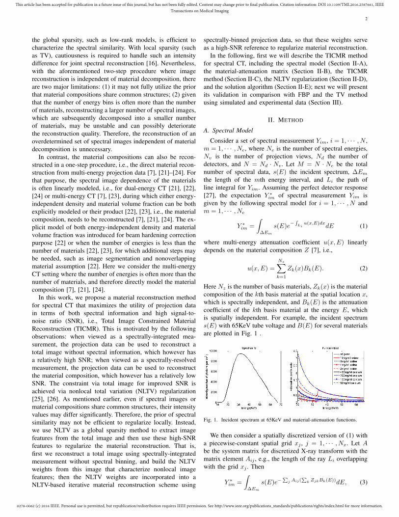
Here Nz is the number of basis materials, Zk(x) is the materialcomposition of the kth basis material at the spatial location x,which is spectrally independent, and Bk(E) is the attenuationcoefficient of the kth basis material at the energy E, whichis spatially independent. For example, the incident spectrums(E) with 65KeV tube voltage and B(E) for several materialsare plotted in Fig. 1 .

Fig. 1. Incident spectrum at 65KeV and material-attenuation functions.

We then consider a spatially discretized version of (1) witha piecewise-constant spatial grid xj , j = 1, · · · , Nx. Let Abe the system matrix for discretized X-ray transform with thematrix element Aij , e.g., the length of the ray Li overlappingwith the grid xj . Then

Y ∗im =

∫∆Em

s(E)e−∑j Aij(

∑k ZjkBk(E))dE, (3)



3

where Zjk is the kth material composition at the grid xj .Next we introduce the effective attenuation coefficient Bkm

of the kth basis material for the energy interval ∆Em, i.e.,

Y ∗im = sme−

∑j Aij(

∑k ZjkBkm), (4)

wheresm =

∫∆Em

s(E)dE. (5)

Here (4) is justified by the mean value theorem for definiteintegrals, thanks to the continuity of B(E) with respect to E.

In the matrix notation, (4) is

Y ∗ = S · e−AZB , (6)

where Y ∗ ∈ RM is the column vector of spectral measuremen-t, S ∈ RM the column vector of source spectrum distributionformed by replicating sm in spatial dimension, A ∈ RN×Nx

the system matrix, Z ∈ RNx×Nz the material composition, andB ∈ RNz×Ne the material-attenuation matrix.

Last, assuming Poisson distribution for Y , we consider thefollowing maximum likelihood function to infer Z for Y ,

p(Y |Z) =∏i,m

(Y ∗im)Yim

Yim!e−Y

∗im , (7)

and particularly its logarithmic version

−ln(p(Y |Z)) =1

2

∑i,m

(Yim([AZB]im−ln(smYim

))2)+C, (8)

where we have applied a second-order Taylor expansion fore−[AZB]im [28], [·]im denotes the matrix element, and Ccontains the terms that are independent of Z.

Thus our spectral model to reconstruct material compositionZ from spectral measurement Y , i.e., the data fidelity term,can be formulated as the following quadratic functional

L(Z) =1

2(AZB − P )TW (AZB − P ) =

1

2‖AZB − P‖2W ,

(9)where P = ln( S

Y ) ∈ RM and W = diag(Y ) ∈ RM×M .

B. Material-Attenuation Matrix

Here we consider how to determine the material-attenuationmatrix Bkm. Based on the previous derivation from Bk(E) toBkm in (4), we have

AZB = P. (10)

Assuming Z is known for the calibration purpose, we cancompute B by solving the overdetermined linear system (10).

Alternatively, we rewrite (10) as∑j

Aij(∑k

ZjkBkm) =

− ln

∫∆Em

s(E)e−∑j Aij(

∑k ZjkBk(E))dE

sm. (11)

Now considering a unit circular/spherical domain of the kthmaterial, (11) is reduced to

Bkm = −ln

∫∆Em

s(E)e−Bk(E)dE

sm. (12)

Given the material-attenuation function B(E) (e.g., Fig. 1),the material-attenuation matrix B can be efficiently computedby (12).

Here the effective discrete material-attenuation matrix Bmodels the spectral dependence of attenuation coefficients foreach material that reduces or alleviates the beam-hardeningartifact. However, when only a limited number of energy binsare available, the energy windows ∆Em, i.e., the integrationlimits for each bin, need to be properly chosen, in order forB to capture the sharp spectral changes, such as the K-edge.

C. Total Image Constrained Material Reconstruction

The proposed TICMR consists of two steps: (i) to recon-struct a total image using spectrally-integrated measurementwithout spectral binning, and build the NLTV weights fromthis image that characterize nonlocal image features; (ii) to in-corporate these NLTV weights computed from high-SNR totalimage into material reconstruction using spectrally-resolvedprojection data.

Let Y0 be the spectrally-integrated measurement, i.e., Y0i =∑m Yim, i = 1, · · · , N . Then the total image X∗ ∈ RNx is

reconstructed by either filtered backprojection (FBP) or thefollowing TV based iterative method

X∗ = arg minX

1

2‖AX − P0‖2W0

+ λ|∇X|1 (13)

where P0 = ln( s0

Y0) ∈ RN with total source energy s0 =∑

m sm, W0 = diag(Y0) ∈ RN×N , and |∇X|1 an isotropicTV norm with regularization parameter λ, e.g.,

|∇X|1 =√∂2xX + ∂2

yX. (14)

Then the material composition Z∗ is reconstructed by thefollowing NLTV based iterative method

Z∗ = arg minZ

1

2‖AZB − P‖2W + λ|∇wZ|1 (15)

where |∇wZ|1 is the NLTV norm that will be given in thenext section.

To summarize, TICMR is achieved in this work throughthe NLTV regularization, during which the total image X∗

reconstructed by FBP or TV (13) provides high-SNR NLTVweights for the material reconstruction of Z∗ by (16).

Note that the NLTV regularization in (16) is quite error-forgiving as the weights involve the averaging with Gaussiankernel (18). As a result, the proposed TICMR method is notsensitive to the beam-hardening artifact that may be presentin the total image (see Fig. 3(a) and 4(c)). In addition, forthe ”invisible” object on the total image that is visible on thespectral image (e.g., Object 3 in Fig. 2), TICMR does notdecrease the reconstruction quality (see Fig. 5), although itdoes not increase the reconstruction quality either since noinformation is provided by the total image.

In practice, we may consider the following constrainedmaterial decomposition model

Z∗ = arg minZ

12‖AZB − P‖

2W + λ|∇wZ|1

s.t.ZC = D,L ≤ Z ≤ U.(16)



4

For example, ZC = D may refer to the constraint where thesummation of all material compositions is equal to one in theregion-of-interest and zero otherwise.

In the result section, we compare TICMR with FBP and thefollowing TV based material reconstruction

Z∗ = arg minZ

12‖AZB − P‖

2W + λ|∇Z|1.

s.t.ZC = D,L ≤ Z ≤ U.(17)

Note that in terms of the regularization in (17), the alternativestrategies can be used, such as tensor framelet transform (asa natural high-order generalization of isotropic TV) [3], [11],[29]–[31], and low-rank models [7], [10], [15], [32], [33].

D. Nonlocal Total Variation

An essential component of NLTV is to characterize thepatch-by-patch similarity [34] instead of pixel-by-pixel sim-ilarity (e.g., TV). That is, for a given image X , the followingweights can be constructed between any two spatial node xand y,

wX(x, y) = e−∫Ω1

Gσ(t)(X(y+t)−X(x+t))2dt

σ2 , (18)

where G is a Gaussian kernel with the standard deviation σ,and Ω1 represents the spatial neighborhood to be comparedaround x and y.

Such a patch-by-patch similarity at the spatial grid x froma high-SNR image X can be used to regularize the low-SNRimage u via the following nonlocal gradient at x [25], i.e.,

∇wu(x, y) = (u(y)− u(x))√wX(x, y),∀y ∈ Ω2. (19)

Here Ω2 is the spatial neighborhood around x where thenonlocal gradient ∇wu(x, y) is computed by (19).

Then the NLTV norm of Z in (16) is given by

|∇wZ|1 =∑k

|∇wZk|1, (20)

where the nonlocal weights w are constructed based on thetotal image X∗ reconstructed from (13).

On the other hand, we need to compute the adjoint of (19)during the reconstruction, for which we utilize the followingadjoint relationship with a nonlocal divergence operator divw

〈∇wu, v〉 = 〈u, divwv〉 (21)

with the nonlocal divergence operator [25] defined as

(divwv)(x, y) =

∫Ω2

(v(x, y)− v(y, x))√wX(x, y)dy (22)

As an illustrative example for discretization of the NLTVtransform and its adjoint, consider a 2D image u ∈ RM×N

with Ω1 = R(2a+1)×(2b+1),Ω2 = R(2m+1)×(2n+1), the refer-ence image X based NLTV weights are defined as

wi,j,k,l = e−

2a,2b∑t1=0,t2=0

Gσ(t1,t2)(Xi−a+t1,j−b+t2−Xk−a+t1,l−b+t2 )2

σ2 ,

for i, k = 1, · · · ,M, j, l = 1, · · · , N, (23)

and the nonlocal gradient ∇wu ∈ RM×N×(2m+1)×(2n+1) canbe defined as

[∇wu]i,j,:,: =

√wi−m,j−n,i,j(ui−m,j−n − ui,j)√

wi−m+1,j−n,i,j(ui−m+1,j−n − ui,j)· · ·√

wi+m,j−n,i,j(ui+m,j−n − ui,j)

· · · √wi−m,j+n,i,j(ui−m,j+n − ui,j)

· · · √wi−m+1,j+n,i,j(ui−m+1,j+n − ui,j)· · · · · ·· · · √

wi+m,j+n,i,j(ui+m,j+n − ui,j)

(24)

where [∇wu]i,j,:,: is the (two-dimensional) submatrix obtainedby staking the third and fourth dimensions of ∇wu at each ithposition in the first dimension and jth in the second dimension,and its adjoint divw(∇wu) ∈ RM×N is

[divw(∇wu)]i,j

=

2m+1,2n+1∑t1=1,t2=1

√wi,j,i−(m+1)+t1,j−(n+1)+t2([∇wu]i,j,t1,t2

− [∇wu]i−(m+1)+t1,j−(n+1)+t2,t1,t2). (25)

In this work we empirically set a = b = 3, m = n = 5.

E. Solution AlgorithmThe solution algorithm for sparsity-based reconstruction

problems (13), (16), and (17) is based on alternating directionmethod of multipliers [35] or split Bregman method [36]. Herewe give the details for solving (16).

In order to solve this L1-type problem (16) with non-differentiable L1 norm, we introduce a dummy variable d =∇wZ to decouple the sparsity regularization from the datafidelity and another dummy variable z = Z to decouple theinequality constraint, i.e.,

minZ,d,z

12‖AZB − P‖

2W + λ|d|1

s.t.ZC = D,∇wZ = d, Z = z, L ≤ z ≤ U.(26)

Then the augmented Lagrangian of (26) is

L(Z, d, z) =1

2‖AZB − P‖2W +

µ1

2‖ZC −D + f1‖22

+µ2

2‖∇wZ − d+ f2‖22 +

µ3

2‖Z − z + f3‖22 + λ|d|1.

(27)

To obtain saddle points of the augmented Lagrangian (27)based on ADMM is to iteratively solve

Zk+1 = arg minZL(Z, dk, zk)

dk+1 = arg mindL(Zk+1, d, zk)

zk+1 = arg minzL(Zk+1, dk+1, z)

fk+11 = fk1 + Zk+1C −Dfk+1

2 = fk2 +∇wZk+1 − dk+1

fk+13 = fk3 + Zk+1 − zk+1.

(28)

The optimal condition for the first subproblem in (28)provides

ATW (AZB − P )BT + µ1(ZC −D + fk1 )CT

+µ2divw(∇wZ − dk + fk2 ) + µ3(Z − zk + fk3 ) = 0. (29)



5

The equation (29) is a linear system that can be solved byconjugate gradient method efficiently.

The vector dk+1 in the second subproblem in (28) canbe analytically solved by applying the shrinkage operatorpointwisely

dk+1 = shrink(∇wZk+1 + fk2 ,

λ

µ), (30)

where the operator shrink(x, γ) = x|x| ∗max(|x| − γ, 0).

The vector zk+1 in the third subproblem in (28) canbe analytically solved by applying the restriction operatorpointwisely

zk+1 = Π[L,U ](Zk+1 + fk3 ), (31)

where the operator Π[L,U ](x) = min(max(x, L), U).

III. RESULTS

A. Simulation Results

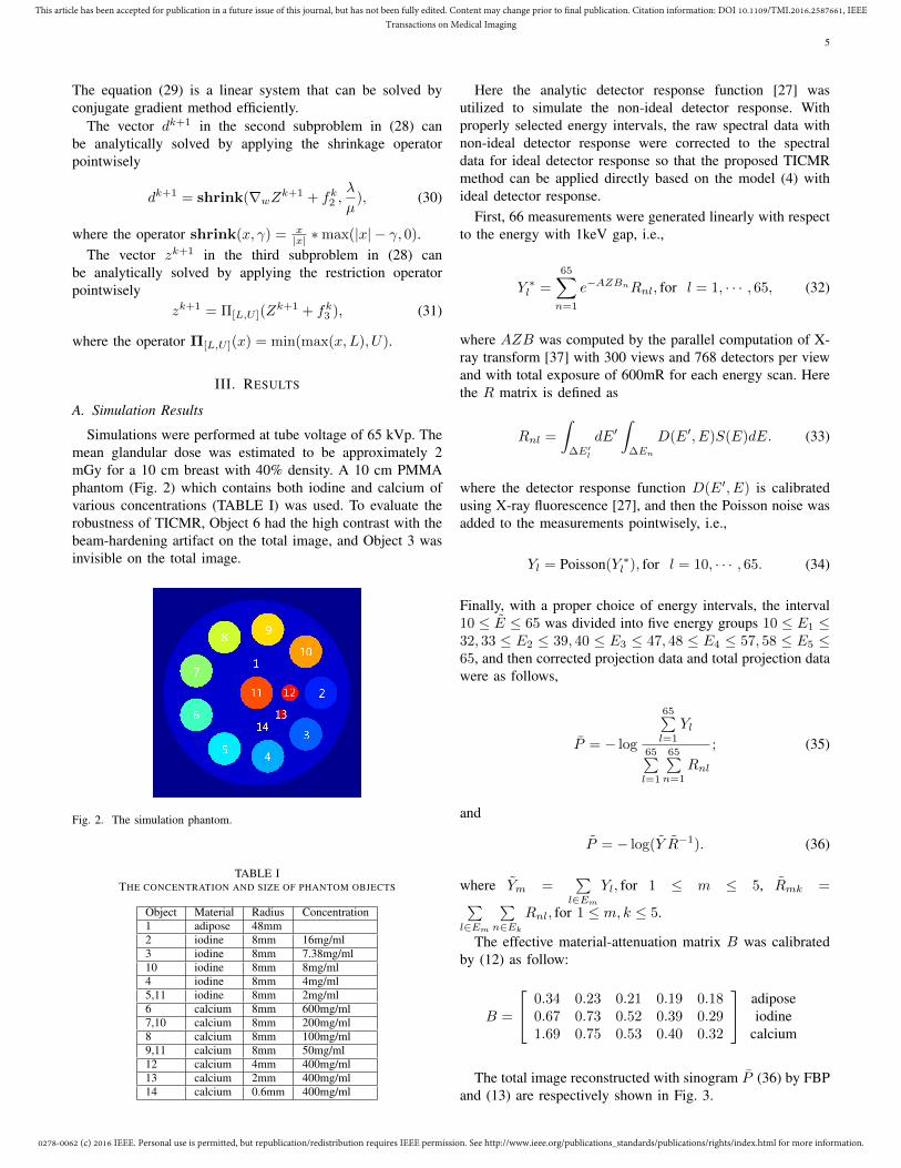
Simulations were performed at tube voltage of 65 kVp. Themean glandular dose was estimated to be approximately 2mGy for a 10 cm breast with 40% density. A 10 cm PMMAphantom (Fig. 2) which contains both iodine and calcium ofvarious concentrations (TABLE I) was used. To evaluate therobustness of TICMR, Object 6 had the high contrast with thebeam-hardening artifact on the total image, and Object 3 wasinvisible on the total image.

Fig. 2. The simulation phantom.

TABLE ITHE CONCENTRATION AND SIZE OF PHANTOM OBJECTS

Object Material Radius Concentration1 adipose 48mm2 iodine 8mm 16mg/ml3 iodine 8mm 7.38mg/ml10 iodine 8mm 8mg/ml4 iodine 8mm 4mg/ml5,11 iodine 8mm 2mg/ml6 calcium 8mm 600mg/ml7,10 calcium 8mm 200mg/ml8 calcium 8mm 100mg/ml9,11 calcium 8mm 50mg/ml12 calcium 4mm 400mg/ml13 calcium 2mm 400mg/ml14 calcium 0.6mm 400mg/ml

Here the analytic detector response function [27] wasutilized to simulate the non-ideal detector response. Withproperly selected energy intervals, the raw spectral data withnon-ideal detector response were corrected to the spectraldata for ideal detector response so that the proposed TICMRmethod can be applied directly based on the model (4) withideal detector response.

First, 66 measurements were generated linearly with respectto the energy with 1keV gap, i.e.,

Y ∗l =65∑

n=1

e−AZBnRnl, for l = 1, · · · , 65, (32)

where AZB was computed by the parallel computation of X-ray transform [37] with 300 views and 768 detectors per viewand with total exposure of 600mR for each energy scan. Herethe R matrix is defined as

Rnl =

∫∆E′l

dE′∫

∆En

D(E′, E)S(E)dE. (33)

where the detector response function D(E′, E) is calibratedusing X-ray fluorescence [27], and then the Poisson noise wasadded to the measurements pointwisely, i.e.,

Yl = Poisson(Y ∗l ), for l = 10, · · · , 65. (34)

Finally, with a proper choice of energy intervals, the interval10 ≤ E ≤ 65 was divided into five energy groups 10 ≤ E1 ≤32, 33 ≤ E2 ≤ 39, 40 ≤ E3 ≤ 47, 48 ≤ E4 ≤ 57, 58 ≤ E5 ≤65, and then corrected projection data and total projection datawere as follows,

P = − log

65∑l=1

Yl

65∑l=1

65∑n=1

Rnl

; (35)

and

P = − log(Y R−1). (36)

where Ym =∑

l∈EmYl, for 1 ≤ m ≤ 5, Rmk =∑

l∈Em

∑n∈Ek

Rnl, for 1 ≤ m, k ≤ 5.

The effective material-attenuation matrix B was calibratedby (12) as follow:

B =

0.34 0.23 0.21 0.19 0.180.67 0.73 0.52 0.39 0.291.69 0.75 0.53 0.40 0.32

adiposeiodine

calcium

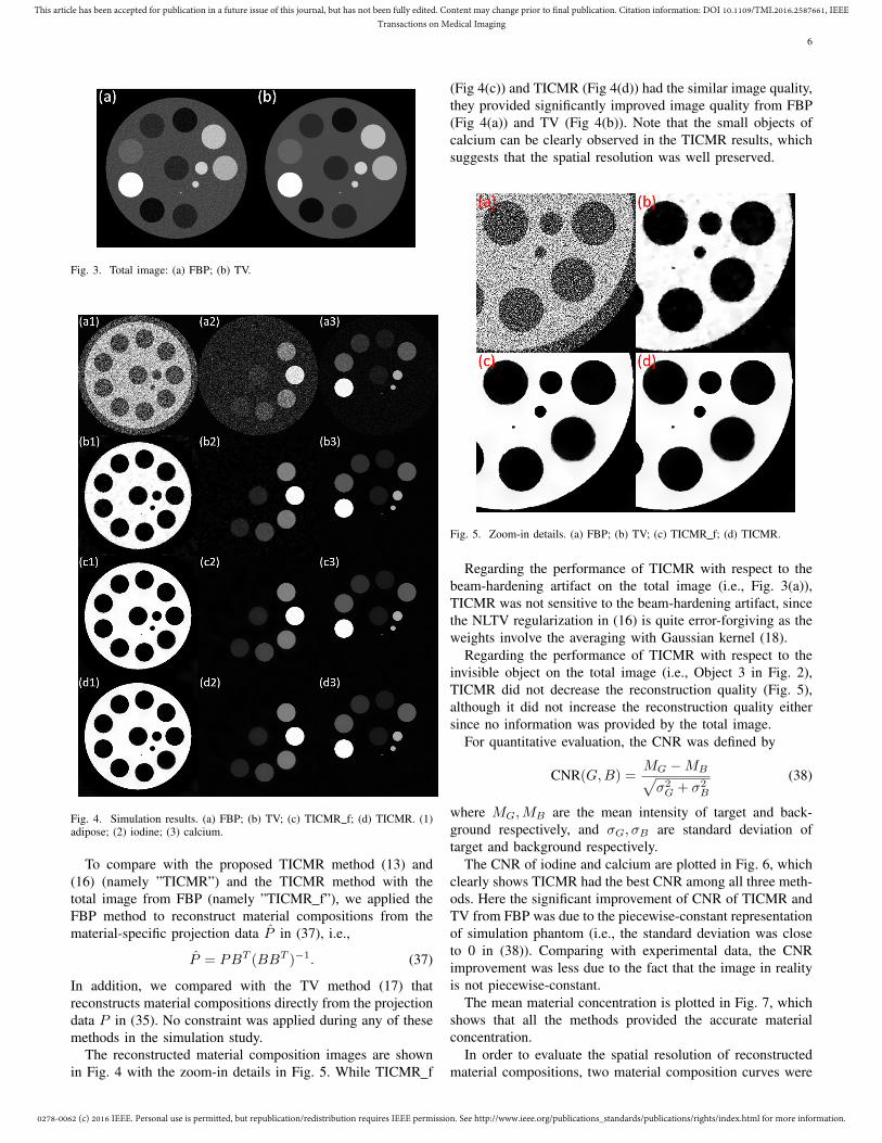
The total image reconstructed with sinogram P (36) by FBPand (13) are respectively shown in Fig. 3.



6

Fig. 3. Total image: (a) FBP; (b) TV.

Fig. 4. Simulation results. (a) FBP; (b) TV; (c) TICMR f; (d) TICMR. (1)adipose; (2) iodine; (3) calcium.

To compare with the proposed TICMR method (13) and(16) (namely ”TICMR”) and the TICMR method with thetotal image from FBP (namely ”TICMR f”), we applied theFBP method to reconstruct material compositions from thematerial-specific projection data P in (37), i.e.,

P = PBT (BBT )−1. (37)

In addition, we compared with the TV method (17) thatreconstructs material compositions directly from the projectiondata P in (35). No constraint was applied during any of thesemethods in the simulation study.

The reconstructed material composition images are shownin Fig. 4 with the zoom-in details in Fig. 5. While TICMR f

(Fig 4(c)) and TICMR (Fig 4(d)) had the similar image quality,they provided significantly improved image quality from FBP(Fig 4(a)) and TV (Fig 4(b)). Note that the small objects ofcalcium can be clearly observed in the TICMR results, whichsuggests that the spatial resolution was well preserved.

Fig. 5. Zoom-in details. (a) FBP; (b) TV; (c) TICMR f; (d) TICMR.

Regarding the performance of TICMR with respect to thebeam-hardening artifact on the total image (i.e., Fig. 3(a)),TICMR was not sensitive to the beam-hardening artifact, sincethe NLTV regularization in (16) is quite error-forgiving as theweights involve the averaging with Gaussian kernel (18).

Regarding the performance of TICMR with respect to theinvisible object on the total image (i.e., Object 3 in Fig. 2),TICMR did not decrease the reconstruction quality (Fig. 5),although it did not increase the reconstruction quality eithersince no information was provided by the total image.

For quantitative evaluation, the CNR was defined by

CNR(G,B) =MG −MB√σ2G + σ2

B

(38)

where MG,MB are the mean intensity of target and back-ground respectively, and σG, σB are standard deviation oftarget and background respectively.

The CNR of iodine and calcium are plotted in Fig. 6, whichclearly shows TICMR had the best CNR among all three meth-ods. Here the significant improvement of CNR of TICMR andTV from FBP was due to the piecewise-constant representationof simulation phantom (i.e., the standard deviation was closeto 0 in (38)). Comparing with experimental data, the CNRimprovement was less due to the fact that the image in realityis not piecewise-constant.

The mean material concentration is plotted in Fig. 7, whichshows that all the methods provided the accurate materialconcentration.

In order to evaluate the spatial resolution of reconstructedmaterial compositions, two material composition curves were



7

drawn along the horizontal and central line passing throughObject 11 as shown in Fig. 8, which suggest that the TICMRhad the best spatial resolution.

Fig. 6. Left: CNR of iodine (object 2-5); right: CNR of calcium (object 6-9).

Fig. 7. Left: material concentration of iodine (object 2-5); right: materialconcentration of calcium (object 6-9).

Fig. 8. Material composition curve along the horizontal and central linepassing through Object 11. Left: iodine; right: calcium.

To summarize, the TICMR result had not only the highestSNR, but also the best spatial resolution. This is enabledby high-SNR total image constrained material reconstructionthrough the NLTV regularization.

B. Experimental Results

Both the calibration phantom data and the postmortembreast tissue data were acquired with a spectral CT systembased on a CZT photon-counting detector at a mean glandulardose of 1.2 mGy. All X-ray photons interacting with the CZTdetector were sorted into five user-definable energy bins.

For quantitative analysis, the calibration phantom (Fig. 9(a))had two inner circles with the water at the top and thelipid at the bottom and its outer circle was filled with theprotein. As a result, the material composition was one in theregion-of-interest and zero otherwise. Here we applied twoconstraints in FBP material decomposition method and all

iterative reconstruction methods: ZC = D where the sumof material compositions is equal to one in the region-of-interest and zero otherwise, and L ≤ Z ≤ U with L = 0and U = 1. The B matrix was obtained using another slice inthe calibration phantom data that was distinct from the sliceas shown in Fig. 9(a).

The total image reconstructed with all projection data by(13) is shown in Fig. 9. The reconstructed material composi-tions are shown in Fig. 10 and Fig. 12 for calibration phantomand breast tissue respectively, which again show that TICMRhad improved image quality from FBP and TV. Note that theprotein composition in the postmortem breast tissue is muchlower than water or lipid.

Fig. 9. Total image for experimental data: (a) calibration phantom; (b) breasttissue.

Fig. 10. Experimental results for calibration phantom. (a) FBP; (b) TV; (c)TICMR. (1) protein; (2) water; (3) lipid.

For calibration phantom, since the ground truth was known,the means in the ROI were summarized in TABLE II, and thespatial profile of two red lines in Fig. 10 is plotted in Fig. 11,which demonstrates that TICMR had improved image qualityfrom FBP and TV in comparison with the ground truth. In



8

addition, the CNR was computed as shown in TABLE III.For breast tissue, only the CNR was computed as shown inTABLE IV, i.e., CNR(ROI2, ROI1) and CNR(ROI3, ROI1)for water and lipid respectively with ROI’s drawn in Fig. 12.

TABLE IITHE MEAN RESULTS FOR CALIBRATION PHANTOM

Material Ground Truth FBP TV TICMRprotein 1.000 0.982 0.981 0.996water 1.000 0.984 1.017 1.011lipid 1.000 1.039 1.034 1.030

TABLE IIITHE CNR RESULTS FOR CALIBRATION PHANTOM

Material FBP TV TICMRwater 16.26 31.42 45.48lipid 1.26 1.51 2.24

Fig. 11. Material composition profile along the line L1 and L2 in Fig. 10.Left: water(L1); right: lipid(L2).

Fig. 12. Experimental results for breast tissue. (a) FBP; (b) TV; (c) TICMR.(1) protein; (2) water; (3) lipid.

TABLE IVTHE CNR RESULTS FOR BREAST TISSUE

Material FBP TV TICMRwater 11.67 20.16 23.78lipid 12.33 16.34 18.89

IV. CONCLUSION

TICMR is proposed for spectral CT with improved im-age quality, i.e., both CNR and spatial resolution. Such animprovement is enabled by the total image constraint viathe NLTV regularization. That is, a high-SNR total image isfirst reconstructed with energy-integrated projection data ofrelatively high SNR, and then built into the NLTV weightsto regularize the material reconstruction with energy-resolvedprojection data of relatively low SNR via the NLTV regular-ization.

V. ACKNOWLEDGEMENT

The authors are grateful to the reviewers and editors fortheir valuable comments. Jiulong Liu and Hao Gao werepartially supported by the NSFC (#11405105), the 973 Pro-gram (#2015CB856000), and the Shanghai Pujiang Talent Pro-gram (#14PJ1404500). Xiaoqun Zhang was partially supportedby the NSFC (#91330102, #GZ1025) and the 973 Program(#2015CB856000). Huanjun Ding and Sabee Molloi werepartially supported by the NIH/NCI (#R01CA13687).

REFERENCES

[1] Kalender et al, Eur. Radiol., 22 1-8, 2012.[2] Ding et al, Radiology, 272 731-738, 2014.[3] Ding et al, Phys. Med. Biol., 59 6005-6017, 2014.[4] Roessl et al, Phys. Med. Biol., 52 4679-4696, 2007.[5] Bornefalk et al, Phys. Med. Biol., 55 1999-2022, 2010.[6] Schmidt, Med. Phys., 36 3018-3027, 2009.[7] Gao et al, Inverse Problems, 27 115012, 2011.[8] Leng et al, Med. Phys., 38 4946-4957, 2011.[9] Zhao et al, Phys. Med. Biol., 57 8217-8229, 2012.[10] Li et al, Journal of X-ray Science and Technology, 2 147-163, 2013.[11] Zhao et al, Med. Phys., 40 031905, 2013.[12] Clark et al, Phys. Med. Biol., 59 6445-6466, 2014.[13] Manhart et al, Proc CT Meet, 91-94, 2014.[14] Xi et al, IEEE Trans. Med. Imag., 34 769-778, 2015.[15] Kim et al, IEEE Trans. Med. Imag., 34 748-760, 2015.[16] Shen et al, Med. Phys., 42 282-296, 2015.[17] Alvarez et al, Phys. Med. Biol., 21 733-744, 1976.[18] Schirra et al, IEEE Trans. Med. Imag., 32 1249-1257, 2013.[19] Xu et al, Phys. Med. Biol., 59 N65-N79, 2014.[20] Taguchi et al, Med. Phys., 40 100901, 2013.[21] Sukovic et al, IEEE Trans. Med. Imag., 19 1075-1081, 2000.[22] Elbakri et al, IEEE Trans. Med. Imag., 21 89-99, 2002.[23] Long et al, IEEE Trans. Med. Imag., 33 1614-1626, 2014.[24] Zhao et al, IEEE Trans. Med. Imag., 34 761-768, 2015.[25] Gilboa et al, Multiscale Modeling and Simulation, 7 1005-1028, 2008.[26] Zhang et al, SIAM Journal on Imaging Sciences , 3 253-276, 2010.[27] Ding et al, Med. Phys., 41 121902, 2014.[28] Sauer et al, IEEE Trans. Signal Processing, 41 534-548, 1993.[29] Gao et al, Med. Phys., 39 6943-6946, 2012.[30] Gao et al, Med. Phys., 40 081919, 2013.[31] Zhou et al, Inverse Problems, 29 125006, 2013.[32] Gao et al, Phys. Med. Biol., 56, 3181, 2011.[33] Cai et al, IEEE Trans. Med. Imag., 33 1581-1591, 2014.[34] Buades et al, Multiscale Modeling & Simulation, 4 490-530, 2005.[35] Boyd et al, Foundations and Trends in Machine Learning, 3 1-122, 2011.[36] Goldstein et al, SIAM Journal on Imaging Sciences, 2 323-343, 2009.[37] Gao, Med. Phys., 39 7110-7120, 2012.

Date post:	14-Apr-2019
Category:	Documents
Upload:	dangxuyen
View:	214 times
Download:	0 times

TICMR: Total Image Constrained Material Reconstruction via...

Documents