TIME-DEPENDENT DIFFUSION MODELS FOR TERM STRUCTURE...

Statistica Sinica 13(2003), 965-992

TIME-DEPENDENT DIFFUSION MODELS FOR TERM

STRUCTURE DYNAMICS

Jianqing Fan, Jiancheng Jiang, Chunming Zhang and Zhenwei Zhou

Chinese University of Hong Kong, Peking University,University of Wisconsin Madison and University of California Los Angeles

Abstract: In an effort to capture the time variation on the instantaneous return and

volatility functions, a family of time-dependent diffusion processes is introduced to

model the term structure dynamics. This allows one to examine how the instanta-

neous return and price volatility change over time and price level. Nonparametric

techniques, based on kernel regression, are used to estimate the time-varying co-

efficient functions in the drift and diffusion. The newly proposed semiparametric

model includes most of the well-known short-term interest rate models, such as

those proposed by Cox, Ingersoll and Ross (1985) and Chan, Karolyi, Longstaff

and Sanders (1992). It can be used to test the goodness-of-fit of these famous

time-homogeneous short rate models. The newly proposed method complements

the time-homogeneous nonparametric estimation techniques of Stanton (1997) and

Fan and Yao (1998), and is shown through simulations to truly capture the het-

eroscedasticity and time-inhomogeneous structure in volatility. A family of new

statistics is introduced to test whether the time-homogeneous models adequately

fit interest rates for certain periods of the economy. We illustrate the new methods

by using weekly three-month treasury bill data.

Key words and phrases: Diffusion model, kernel regression, nonparametric goodness-

of-fit.

1. Introduction

The theory of pricing contingent claims is one of the most celebrated math-ematical results in finance. It offers valuable practical guidance for asset valu-ation and risk managements. An excellent introductory treatment of this is inHull (1997), and more rigorous accounts can be found in Merton (1992), Duffie(1996), among others. The short-term riskless interest rates are fundamental andimportant in financial markets. They are directly related to consumer spending,corporate earnings, asset pricing, inflation and the overall economy. See Mishkin(1997) for further discussions. Many useful short-rate models have been pro-posed to explain term-structure dynamics and other issues in finance. See forexample Merton (1973), Vasicek (1977), Dothan (1978), Brennan and Schwartz(1979, 1980), Cox, Ingersoll and Ross (1980, 1985), Constantinides and Ingersoll

966 JIANQING FAN, JIANCHENG JIANG, CHUNMING ZHANG AND ZHENWEI ZHOU

(1984), Schaefer and Schwartz (1984), Feldman (1989), Longstaff (1989), Hulland White (1990), Black and Karasinski (1991), Longstaff and Schwartz (1992),Chan, Karolyi, Longstaff and Sanders (1992), Hansen and Scheinkman (1995),Andersen and Lund (1996), Gallant and Tauchen (1997, 1998), Gallant, Rossiand Tauchen (1997), Aıt-Sahalia (1996a, 1996b), Stutzer (1996), Stanton (1997),Aıt-Sahalia and Lo (1998), among others. These models provide useful insightsinto the term structure dynamics.

Modern asset pricing theory allows one to value and hedge contingent claims,once a model for the dynamics of an underlying state variable is given. Many suchmodels have been developed, such as the geometric Brownian motion (Black andScholes (1973)) and the interest-rate models mentioned in the last paragraph.Most of these are simple and convenient time-homogeneous parametric models,attempting to capture certain salient features of observed dynamic movements.However, they are not fully derived from any economic theory and cannot beexpected to fit all financial data well. Thus, while the pricing theory gives usspectacularly beautiful formulas when an underlying dynamic is correctly mod-eled, it offers little guidance in choosing a correct model or validating a specificparametric model. Hence there is a possibility that misspecification of a modelleads to erroneous valuation and hedging. This motivates us to consider a largeclass of nonparametric and semiparametric models. An advantage of such mod-els is that they reduce possible modeling biases and can be used to build andvalidate a parametric model. This allows us to better explore the explanatorypower of parametric approaches by means of nonparametric validation methods.

Economic conditions change from time to time. Thus, it is reasonable to ex-pect that the instantaneous expected return and volatility depend on both timeand price level for a given state variable, such as stock prices and bond yields. Itis difficult, however, to precisely describe how the bivariate functions for the ex-pected return and volatility vary over time and price level. Restrictive functionalforms of expected return and volatility can create large biases for different assetswithin certain period. The most flexible model is not to assume any specificforms of the bivariate functions, but to let the data themselves determine appro-priate forms that describe the dynamics. Such a data-analytic approach is callednonparametric regression in the statistical literature. For an overview of non-parametric methods, see recent books by Hastie and Tibshirani (1990), Hardle(1990), Scott (1992), Green and Silverman (1995), Simonoff (1995) and Fan andGijbels (1996). However, as we explain in Section 2, there is not sufficient in-formation to determine nonparametrically the bivariate functions. Hence, someform of the instantaneous return and volatility functions should be imposed.

In an attempt to capture time variation on the instantaneous return andprice volatility, we expand the interest rate model of Chan et al. (1992) in two

TIME-DEPENDENT DIFFUSION MODELS FOR TERM STRUCTURE DYNAMICS 967

important aspects: we allow coefficients to change smoothly over time and wepermit a transform of the state variable to enter into the equation. This semipara-metric model enables one to simultaneously capture the time effect and reducemodeling bias. These functions in the semiparametric model can be estimatedwith reasonable accuracy, because of the availability of data, such as the yieldsof treasury bills and stock price indices over a long period. In other words, byusing semiparametric and nonparametric models, we reduce model bias withoutexcessively inflating the variance of the estimated functions.

The nonparametric techniques that we employ here are based on local con-stant fit (which is for simplicity, one can also use the popular local linear fit orlocal polynomial fit) with left-sided kernels. While the local linear fit has sometheoretical advantages (Fan and Gijbels (1996)), our experience shows that it cancreate some artificial, statistically insignificant time trend. Compared with thetraditional two-sided kernel methods, the one-sided kernel allows one to estimatea function, at any point in its support, using only historical observations. Thismodification makes prediction much easier.

As in all nonparametric approaches, our techniques require selection of thebandwidth. Popular methods include cross-validation (Stone (1974)), general-ized cross-validation (Wahba (1977)), the pre-asymptotic substitution method(Fan and Gijbels (1995)) and the plug-in method (Ruppert, Sheather and Wand(1995)). Our bandwidth selection method is to minimize overall prediction errors,thanks to the one-sided kernel methods which facilitate the prediction.

Our time-dependent semiparametric model contains most of the well-knownparametric models for interest rate dynamics. This allows us to test whether aparticular parametric model fits a given dataset, regarding the semiparametricmodel as an alternative. Our testing procedure is based on a generalized pseudo-likelihood ratio test. It is shown in Fan, Zhang and Zhang (2001) that this testpossesses a number of good statistical properties. In our current applications, abootstrap method is used to estimate the null distribution of the test statistic. Weapply the techniques to test various parametric models. Similar to the conclusionsof Chan et al. (1992) and Gallant, Long and Tauchen (1997), all these parametricmodels have very small P -values and strong evidence for lack of fit.

2. Method of Estimation

In valuing contingent claims, it is frequently assumed that an underlyingstate variable, Xt, satisfies a time-dependent continuous-time stochastic differ-ential equation:

dXt = µ(t,Xt) dt + σ(t,Xt) dWt. (1)


Here Wt denotes the standard Brownian motion and the bivariate functionsµ(t,Xt) and σ(t,Xt) are called the drift and diffusion of the process {Xt}, re-spectively (Wong (1970) and Duffie (1996)). Note that

µ(t,Xt) = lim∆→0

1∆

E(Xt+∆−Xt|Xt), and σ2(t,Xt) = lim∆→0

1∆

E{(Xt+∆−Xt)2|Xt}.(2)

Examples of (1) include geometric Brownian motion (GBM) for stock prices, andthe interest rate models of Merton (1970), Vasicek (VAS) (1977), Cox, Ingersolland Ross (CIR VR) (1980), Cox, Ingersoll and Ross (CIR SR) (1985), ChanKarolyi, Longstaff and Sanders (CKLS) (1992), among others. Different modelspostulate different forms of µ and σ, for instance,

GBM: dXt = µXt dt + σXt dWt,

VAS: dXt = (α0 + α1Xt) dt + σ dWt,

CIR VR: dXt = σXt3/2 dWt,

CIR SR: dXt = (α0 + α1Xt) dt + σ√

Xt dWt,

CKLS: dXt = (α0 + α1Xt) dt + σXγt dWt.

These time-homogeneous models are a specific family of the nonparametric mod-els,

dXt = µ(Xt) dt + σ(Xt) dWt, (3)

studied by Stanton (1997), Fan and Yao (1998) and Chapman and Pearson(2000), where the functional forms of µ and σ are unspecified.

2.1. Time-dependent diffusion models

It is reasonable to expect that the instantaneous return and volatility slowlyevolve with time. Time-homogeneous models, while useful, are not capable ofcapturing this kind of feature. In fact, it is common practice to apply parametricmodels to a window of time series (e.g., in 1999, one uses only data between 1995and 1999 to estimate parameters in the model), and this window of series movesas time evolves (e.g., in 2002, one would now use the data between 1998 and2002 to estimate parameters). The resulting estimates are time-dependent. Thisin essence utilizes time-dependent parametric techniques with a prescribed timewindow. Various efforts have been made to explicitly express the dependenceof parameters on time. These include the time-dependent models of Ho andLee (HL) (1986), Hull and White (HW) (1990), Black, Derman and Toy (BDT)(1990) and Black and Karasinski (BK) (1991). They assume, respectively, the


following forms:

HL: dXt = µ(t) dt + σ(t) dWt,

HW: dXt = {α0(t) + α1(t)Xt} dt + σ(t)Xti dWt, i = 0 or 0.5,

BDT: dXt = {α1(t)Xt + α2(t)Xt log(Xt)} dt + β0(t)Xt dWt,

BK: dXt = {α1(t)Xt + α2(t)Xt log(Xt)} dt + β0(t)Xt dWt,

where α2(t) =d log{β0(t)}

dt.

These forms are specific examples of the following time-dependent model:

dXt = {α0(t) + α1(t)g(Xt)} dt + β0(t)h(Xt)β1(t) dWt, (4)

for some functions α0, α1, g, β0, β1 and h whose forms are not specified. (TheBDT and BK models can be included in (4) if one uses the transformed variableX∗

t = log(Xt).) Indeed, the time-inhomogeneous nonparametric model (4) in-cludes all of the time-homogeneous and time-inhomogeneous models mentionedabove. For example, the nonparametric model of Stanton (1997) correspondsto (4) with α0(t) = 0, α1(t) = 1, β0(t) = 1 and β1(t) = 1. Model (4) alsoallows one to check whether a particular model is valid or not, via either formalstatistical tests or visual comparisons between parametric and nonparametricfits. It reduces degrees of danger on model misspecification and permits one tochoose a parametric model from nonparametric analyses. This provides a usefulintegration of parametric and nonparametric approaches.

One notable distinction between the models at (1) and (4) is the estimabilityof the parameters in the expected return and volatility. The widest possible one-factor model is the one with the forms of the drift and diffusion in (1) completelyunspecified. However, the drift and diffusion functions are then inestimable,since only a trajectory in the time and state domains is observed. In contrast,the expected return and the volatility functions in the nonparametric model (4)are estimable.

A useful class of (4) specifies the functions g and h. An example of this is

dXt = {α0(t) + α1(t)Xt} dt + β0(t)Xβ1(t)t dWt. (5)

This submodel is an extension of the CKLS model that allows the coefficientsto depend arbitrarily on time. It includes all of the aforementioned parametricmodels, in both time-homogeneous and time-dependent settings. One can alsospecify other forms of g and h, and our techniques continue to apply. Thus,this paper concentrates mainly on model (5). An interesting probabilistic ques-tion is the conditions under which model (5) is arbitrage-free. Sandmann andSondermann (1997) have studied some aspect of this issue.


A further restriction of (5) is to assume that β1(t) = β1 is time-independent.While this imposes certain restrictions, it avoids some collinearity problems inestimating β0(t) and β1(t). The parameter β1 and the coefficient function β0(t)in this parsimonious model can be estimated more reliably. We discuss this issuein Section 6 after we have introduced some necessary tools.

2.2. Estimation of instantaneous return

Assume that the coefficient functions in model (5) are twice continuouslydifferentiable and we are given the data {Xti , i = 1, . . . , n+1} sampled at discretetime points, t1 < · · · < tn+1. In many applications, the time points are equallyspaced. For example, when the time unit is a year, weekly data are sampledat ti = t0 + i/52, i = 1, . . . , n + 1, for a given initial time point t0. Let Yti =Xti+1 −Xti , Zti = Wti+1 −Wti , and ∆i = ti+1− ti. According to the independentincrement property of Brownian motion, the Zti are independent and normallydistributed with mean zero and variance ∆i. Thus the discretized version of (5)can be expressed as

Yti ≈ {α0(ti) + α1(ti)Xti}∆i + β0(ti)Xβ1(ti)ti

√∆i εti , i = 1, . . . , n, (6)

where {εti}ni=1 are independent and standard normal. As pointed out in Chan

et al. (1992) and demonstrated by Stanton (1997), the discretized approximationerror to the continuous-time model is of second order when the data are observedover a short time period. See also the recent work of Aıt-Sahalia (1999, 2002).Indeed, according to Stanton (1997), as long as data are sampled monthly ormore frequently, the errors introduced by using approximations rather than thetrue drift and diffusion are extremely small when compared with the likely size ofestimation errors. Higher order differences, such as those elaborated by Stanton(1997), are also possible. While higher order approximations lead to lower orderapproximation errors, they significantly increase the variance of nonparametricestimators (Fan and Zhang (2003)). An asymptotic analysis in Fan and Zhang(2003) shows that, in the time-homogeneous nonparametric model studied byStanton (1997), the variance inflation factors for estimating the instantaneousreturn (denoted by V1(k)) and squared volatility (denoted by V2(k)) using k-thorder differences are very substantial. Details are excerpted in Table 1. Thismakes higher order approximations less attractive. Thus, for simplicity and forvariance reduction, we opt for the first order difference.

Recall that the forms of the functions α0(t) and α1(t) are not specified. Wecan only use their qualitative features: the functions are smooth so that they canbe locally approximated by a constant. That is, at a given time point t0, we usethe approximation αi(t) ≈ αi(t0), i = 0, 1, for t in a small neighborhood of t0. Leth denote the size of the neighborhood and K be a nonnegative weight function.


These are called a bandwidth parameter and a kernel function, respectively.Following the local regression technique (see Fan and Gijbels (1996)), we canfind estimates of αi(t0), i = 0, 1, via the following (locally) weighted least-squarescriterion: Minimize

n∑i=1

[Yti

∆i− a − bXti

]2Kh(ti − t0) (7)

with respect to parameters a and b, where Kh(·) = K(·/h)/h. Note that when K

has a one-sided support, such as [−1, 0), for example the one-sided Epanechnikovkernel 3/4(1 − t2)I(t < 0) (see Epanechnikov (1969)), the above local constantregression only uses the data observed in the time interval [t0 − h, t0). Thisamounts to using only historical data and is useful for forecasting. It also facil-itates data-driven bandwidth selection. Our experience shows that there is notsignificant difference between nonparametric fitting with one-sided and two-sidedkernels.

Table 1. Variance inflation factors in using higher order differences (fromFan and Zhang (2003)).

Order k 1 2 3 4 5 6 7 8 9 10

V1(k) 1.00 2.50 4.83 9.25 18.95 42.68 105.49 281.65 798.01 2364.63

V2(k) 1.00 3.00 8.00 21.66 61.50 183.40 570.66 1837.28 6076.25 20527.22

Let a and b be the minimizers of the weighted least-squares regression (7).Then, the local estimators of α0(t0) and α1(t0) are α0(t0) = a and α1(t0) = b. Toobtain the estimated functions, α0(·) and α1(·), we usually evaluate the estimatesat hundreds of grid points. Note that we have ignored the heteroscedasticity at(7). In principle, we can incorporate heteroscedasticity via minimizing

n∑i=1

[Yti

∆i− a − bXti

]2β−2

0 (ti)X−2β1(ti)ti Kh(ti − t0), (8)

where β0 and β1 are obtained from the procedure described in the next section.However, we do not experience any substantial gains, due to the large stochasticnoise contaminating the expected return function.

2.3. Estimation of volatility

Let µ(t,Xt) = α0(t) + α1(t)Xt stand for the estimated mean function andset Et = {Yt − µ(t,Xt)∆t}/

√∆t. Then, by (6), we have

Et ≈ β0(t)Xβ1(t)t εt. (9)


Note that this approximation also holds when Et is replaced by Yt/√

∆t, aspointed out by Stanton (1997). However, with Et = {Yt − µ(Xt, t)∆t}/

√∆t,

the approximation error is of smaller order. The conditional log-likelihood of Et

given Xt is, up to an additive constant, approximately expressed as

−12

log{β20(t)X2β1(t)

t } − E2t

2β20(t)X2β1(t)

t

.

Summing it up with respect to t, we obtain the logarithm of the pseudo-likelihood.By using the local constant approximation and introducing the kernel weight weobtain, at a time point t0, the local pseudo-likelihood

�(β0, β1; t0) = −12

n∑i=1

Kh(ti − t0)

(log(β2

0X2β1ti ) +

E2ti

β20X2β1

ti

). (10)

Maximizing (10) with respect to the local parameters β0 and β1, we obtain theestimates β0(t0) = β0, and β1(t0) = β1. The whole functions β0(·) and β1(·)can be estimated by repeatedly maximizing (10) over a grid of time points. Thistype of local pseudo-likelihood method is related to the generalized method ofmoments of Hansen (1982), but is used now in a local neighborhood. See alsoFlorens-Zmirou (1993) and Genon-Catalot and Jacod (1993).

Note that for given β1, the maximization of �(β0, β1; t0) is obtained at

β20(t0;β1) =

n∑i=1

Kh(ti − t0)E2ti |Xti |−2β1

/ n∑i=1

Kh(ti − t0). (11)

Thus, at a point t0, we only need to maximize the one-dimensional function�(β0(t0;β1), β1; t0) with respect to β1. The whole function β1(t) can be obtainedby repeatedly optimizing this one-dimensional function at a grid of time points.Using the estimate β1(tj) as the initial value for maximizing the target function atthe next grid point tj+1, the maximizer can be found within only a few iterations.Thus the computational burden is not much heavier than that for estimating thedrift function. The estimated function β0(t) can be obtained by using (11) ateach grid point.

An alternative approach is to use the local least-squares method by notingthat (9) implies

log(E2t ) ≈ log{β2

0(t)} + β1(t) log(X2t ) + log(ε2

t ). (12)

This is again a semi-parametric model and the method in Section 2.2 for estimat-ing the drift function can be applied to estimate the parameters log{β2

0(t)} andβ1(t). We implemented this method but did not get satisfactory results. This


is mainly due to the exponentiation operation used in the estimation of β20(t),

which inflates (deflates) the estimate substantially.The time-dependent model (5) is also related to a GARCH(1,1) model. To

see this relation, take β1 ≡ 0, so that (5) becomes dXt = {α0(t) + α1(t)Xt} dt +β0(t) dWt, and (11) reduces to β2

0 =∑n

i=1 Kh(ti − t0)E2ti/∑n

i=1 Kh(ti − t0). As-sume ti = ∆i and let ri = Eti , i = 1, . . . , n. To stress the dependency of β0 onthe time point t0, we write it as σt0 . If we take K(x) = axI(x < 0) for someparameter a > 1, then Kh(x) = bxI(x < 0)/h with b = a1/h, which is greaterthan 1. Consequently, it follows that σ2

t =∑

i>0 λir2t−i/

∑i>0 λi, where λ = b−∆.

Note that σ2t = λσ2

t−1 +(1−λ)r2t . This is indeed the J. P. Morgan (1996) estima-

tor for volatility. This estimator can be regarded as the one from a GARCH(1,1)model. In other words, our time-dependent model and the GARCH(1,1) modelhave some intrinsic connections: both of them use the volatility in the recenthistory.

2.4. Bandwidth selection

The bandwidth h in the kernel regression can be tuned to optimize the perfor-mance of the estimated functions. It can be subjectively tuned by users to tradeoff the bias and variance of the nonparametric estimates by visual inspection, orchosen by data to minimize some criteria that are related to the prediction error.

The criteria that we proposed here take advantage of the fact that the one-sided kernel is employed so that only historical data are used in the construc-tion of estimators. The bandwidth for the expected instantaneous return canbe chosen to minimize the average prediction error (APE) as a function of thebandwidth:

APE = m−1m∑

i=1

(Yt∗i − Yt∗i )2

σ2t∗i

,

with Yt∗i = {α0(t∗i ) + α1(t∗i )Xt∗i }∆t∗i and σt∗i = β0(t∗i )Xβ1(t∗i )t∗i

. In the above def-inition, the prediction errors are computed at the prescribed time points t∗i ,i = 1, . . . ,m. This kind of idea has also been used by Hart (1994, 1996).

For estimation of the volatility, since the local pseudo-likelihood is used toconstruct nonparametric estimators, the bandwidth will be chosen to maximizethe pseudo-likelihood of Et given Xt. More specifically, for a given bandwidth h,the pseudo-likelihood function is defined as

−12

m∑i=1

log{β20(t∗i )X

2β1(t∗i )t∗i

} +E2

t∗i

β20(t∗i )X

2β1(t∗i )t∗i

.


2.5. Standard errors

Standard errors of statistical estimators are useful for assessing accuracy.The kernel regression estimators in (7) and (8) are actually weighted least-squares estimators. Thus, traditional linear regression techniques continue toapply. When the data are independent, the formulas for standard errors of thelocal linear estimators are given on page 115 of Fan and Gijbels (1996). Fordependent data, we can use the regression bootstrap (see Franke, Kreiss andMammen (2002)) to assess the sampling variability. The idea is to generate thebootstrap responses {Y ∗

ti} from (6), using the estimated parameter functions and{Xti}, but with the new random shocks {ε∗ti}. Based on the bootstrap sample{(Xti , Y

∗ti ), i = 1, . . . , n}, the coefficient functions are estimated and sampling

variability can be evaluated. In our simulations, the bootstrap confidence inter-vals are calculated based on 1,000 bootstrap samples.

3. Applications and Simulations

In this section, we first apply our proposed techniques to the treasury billdata. After that, we verify our techniques by using two simulated data sets,which are similar to short-rate dynamics.

3.1. Treasury bill data

To understand interest rate dynamics, we use the yields of the three-monthtreasury bill from the secondary market rates on Fridays. The secondary marketrates are annualized using a 360-day year of bank interest and are quoted on adiscount basis. The data consist of 1461 weekly observations, from January 2,1970 to December 26, 1997.

The annualized three-month yields and their weekly rate changes are pre-sented in Figure 1. Figure 2 shows the estimated coefficient functions α0(t),α1(t), β0(t) and β1(t) along with the 95% pointwise confidence bands producedby the bootstrap method. Figure 3 describes how the expected instantaneousreturn and volatility change over time, and also displays their 95% pointwiseconfidence bands. The bandwidths are selected by the methods described inSection 2.4. The heteroscedasticity and time effect on volatility are evident. Acareful inspection of Figure 2 suggests a time effect after 1980, but not before.This is probably due to the fact that the Federal Reserve changed its monetarypolicy on October 6, 1979 when its newly appointed chairman, Paul Volcker,initiated money supply targeting and abandoned interest rate targeting.


Figure 1. Three month treasury Bill rate, from January 2, 1970 to December26, 1997. Annualized yield on three-month treasury bills, January 2, 1970to December 26, 1997. Top panel: Weekly yields. Bottom panel: Changesof weekly yields.

Figure 2. Three month treasury Bill rate. (a) Estimated α0(t) with 95%bootstrap confidence band. (b) Estimated α1(t) with 95% bootstrap confi-dence band. (c) Estimated β0(t) with 95% bootstrap confidence band. (d)Estimated β1(t) with 95% bootstrap confidence band. Solid – estimator,dotted – confidence band.


Figure 3. Three month treasury Bill rate. (a) Estimated drift with 95%bootstrap confidence band. (b) Estimated volatility with 95% bootstrapconfidence band. Solid – estimator, dotted – confidence band.

3.2. Verification of the proposed techniques

We now test our techniques by simulating two data sets from specific modelsof (5). The first one is the time-homogeneous model

dXt = (0.0408 − 0.5921Xt) dt +√

1.6704 X1.4999t dWt. (13)

The values of the parameters are given in Chan et al. (1992), based on one-monthtreasury bill yields. We generate 1,735 weekly observationsn from January 5, 1962to March 31, 1995. Based on 400 simulations, we get the estimators of α0(ti),α1(ti), β0(ti) and β1(ti). Figure 4 reports the pointwise 2.5th, 12.5th, 87.5thand 97.5th sample percentiles. Figure 5 gives the typical estimated drift andvolatility of the rate change, where the typical estimated curves presented havemedian performance in terms of mean squared errors among 400 simulations.We can see that even for the time-independent CKLS model, our techniques cancapture the true structure of the model without “false alarms”, namely, reportingtime-homogeneous models correctly to be time-homogeneous models.

Next, we test our methodology on a time-inhomogeneous model. For sim-plicity we consider model (5) with drift zero, and assume that the coefficientfunctions for volatility contain nonlinear trends as depicted in Figure 7 (see thesolid lines). In order to visually display characteristics of this artificial model,we present in Figure 6 a simulated sample path consisting of 780 weekly obser-vations from the model. Figure 7 displays the fitted coefficient functions for thedata set. In 400 simulations, each containing 780 observations from the model,we compute the nonparametric estimators of the coefficient for each sample.


Figure 4. Envelopes formed via pointwise 2.5th, 12.5th, 87.5th and 97.5thsample percentiles among 400 simulations of model (13). Solid – true curve,dash-dotted – 75% envelopes, dotted – 95% envelopes. (a) α0(t). (b) α1(t).(c) β0(t). (d) β1(t).

Figure 5. Typical estimated drift and volatility of the rate change among400 simulations for model (13). Solid – true, dashed – our estimators.


Figure 6. A simulated data set from model (5) with drift zero and time-inhomogeneous volatility with coefficient functions given in Figure 7.

Figure 7. Estimated coefficient functions for the simulated data set in Figure6. Solid – true curves, dashed – our estimators.

Figure 8 summarizes the simulation results by plotting the pointwise 5th, 12.5th,87.5th and 95th percentiles among 400 simulations. Clearly our time-inhomogeneousmodel (5) does well at capturing the time effect in volatility.


Figure 8. Envelopes for volatility formed via pointwise 5th, 12.5th, 87.5th,and 95th sample percentiles among 400 simulations for model (5). Solid –the true, dash-dotted – 75% envelopes, dotted – 90% envelopes.

3.3. Empirical comparisons

In order to gauge the relative performance among several models, we testtheir forecasting power for the interest rate changes considered in Section 3.1. Inaddition, we test their forecasting power for the squared interest rate changes andfor the logarithm of the squared interest rate changes (the logarithm transformsthe multiplicative model into the additive model as in (12)). This provides sim-ple measures of how well each interest rate model captures the expected returnand volatility. The predictive powers are measured by the correlation coeffi-cient between the rate changes and their conditional expected return, and thecorrelation coefficient between the squared rate changes and their conditionalexpected volatility. Denote by ρ1 and ρ2 the two correlations, respectively. Theyare related to the coefficient of determination R2 used in Chan et al. (1992) viathe simple relation R2 = ρ2. We also denote by ρ∗2 the correlation coefficient be-tween the logarithm of the squared interest rate changes and the logarithm of theconditional expected volatility. These correlation coefficients provide alternativemeasures for model comparisons.

Table 2. Correlation coefficients.

Models Stanton CKLS CIR SR CIR VR VAS GBM Model (5) Model (4)ρ1 0.1005 0.0479 0.0479 0.0479 0.0479 0.0479 0.0726 0.1018ρ2 0.3181 0.3801 0.3411 0.3840 0.0000 0.3656 0.4057 0.3229ρ∗2 0.3012 0.2723 0.2321 0.2723 0.0000 0.2370 0.3215 0.3213

Model (4) with both g(·) and h(·) taken as the estimate from Stanton’s model.


The results are presented in Table 2. It is evident that, from measures ρ2 andρ∗2, our time-dependent model (5) does a better job of capturing the short-ratevolatility than its time-homogeneous counterpart, the CKLS model. In light ofρ1, the measure of predictive power for the drift, model (4) performs the best,followed by Stanton’s model and our model (5). The overall performance of ournonparametric model (5) is the best among all competing models.

4. Goodness-of-Fit Test

There are a number of stimulating interest rate models that capture differentaspects of the term structure dynamics. A question arises naturally: are thesemodels statistically different? That is, given the amount of information in thedata, are they distinguishable? Here, we take the advantage of the fact thatthe time-dependent model (5) includes most of the popular parametric modelsfor interest rates, therefore it can be treated as the alternative hypothesis. Forexample, we may wish to test whether the coefficient functions depend on time.This amounts to testing H0 : α0(t) = α0, α1(t) = α1, β0(t) = β0, β1(t) = β1

under model (5). One can also test whether the interest rate data follows theCIR model by checking H0 : α0(t) = α0, α1(t) = α1, β0(t) = β0, β1(t) = 0.5in model (5). Assessing the adequacy of the geometric Brownian motion can beformulated in a similar manner.

4.1. Generalized pseudo-likelihood ratio test

Due to large stochastic errors in the estimation of the instantaneous returnfunctions, most reasonable models for the drift function will be accepted. For thisreason, we focus on testing the functional forms of the volatility function, thoughthe technique applies to problems of testing the instantaneous return function.

For brevity, we outline a procedure for testing the CKLS model against thetime-dependent model (5). The technique applies equally to testing other formsof parametric models. Consider testing H0 : β0(t) = β0, β1(t) = β1. Under model(5), the logarithm of the pseudo-likelihood is represented by

�(H) = −12

n∑i=1

log{β20(ti)X

2β1(ti)ti } +

E2ti

β20(ti)X

2β1(ti)ti

,

where β0(ti) and β1(ti) are the kernel estimates outlined in Section 2.3. Similarly,under the hypothesis, one can estimate the parameters β0 and β1 by maximizingthe corresponding pseudo-likelihood to obtain

�(H0) = −12

n∑i=1

log(β20X2β1

ti ) +E2

ti

β20X2β1

ti

.


The plausibility of the hypotheses can then be evaluated by

λ(X, h) = 2{�(H) − �(H0)}, (14)

where X denotes the observed data and h is the bandwidth used for the non-parametric estimates. The null hypothesis is rejected when λ(X, h) is too large.

To compute the P -value of the test statistic, we need to find the distributionof λ(X, h) under the hypothesis. The analytic form of the distribution is hard tofind, but the distribution can be estimated by the parametric bootstrap (simu-lation) procedure. Under the hypothesis, the observed data are generated fromthe model

dXt = {α0(t) + α1(t)Xt} dt + β0Xβ1t dWt. (15)

Set the parameters (β0, β1) at their estimated values (β0, β1), and set the func-tions α0(t) and α1(t) at their estimated values or even at the global least-squaresestimates α0 and α1, because of their insignificant influence. Simulate a pseudo-sample path {X∗

ti , i = 1, . . . , n + 1} from (15), and obtain the test statisticλ(X∗, h). Repeating this procedure 1000 times (say), we obtain 1000 statis-tics of λ(X∗, h). The estimated P -value of the test statistic λ(X, h) is simply thepercentage of the simulated statistics {λ(X∗, h)} exceeding the observed value ofλ(X, h).

The theoretical justification of the above parametric bootstrap method isthe so-called Wilks phenomenon (Fan, Zhang and Zhang (2001)). There it isshown that, in somewhat different settings, the asymptotic null distribution ofthe generalized likelihood ratio statistic often does not depend on, to first order,the nuisance parameters under the null hypothesis. Translating this propertyinto our setting, the null distribution of λ(X, h) does not depend heavily on thevalues of α0(t), α1(t), β0 or β1. Setting them at reasonable estimates, such asthose suggested above, the distribution of λ(X, h) is known and can be simulated.

The above technique applies readily to other hypothesis testing problems.For example, to test the CIR model with β1 = 1/2, one can compute the pseudo-likelihood under the null hypothesis using the known value β1 = 1/2. In thebootstrap estimation of the null distribution, the value β1 = 1/2 should also beused directly.

4.2. Power simulation

The purposes of the simulation are two-fold. One is to demonstrate thatour bootstrap method gives the right estimate of the null distribution, and theother is to show the power of our proposed test. For simplicity, we only considerthe simulations for the volatility part. We use the models that are relevant to


the term structure dynamics. The CKLS model is taken as the null hypothesis.Power is evaluated at a sequence of alternatives, ranging from the CKLS model toreasonably far away from it. Let αi(t) and βi(t), i = 0, 1, be the known functionsdefined as in Figure 2 (see the solid lines). Let βi be the corresponding estimatorsof the functions βi(t), i = 0, 1, under the null hypothesis, for the treasury billdata studied in Section 3.1. We evaluate the power of the pseudo-likelihood ratiotest at a sequence of alternative models indexed by θ:

dXt = {α0(t) + α1(t)Xt} dt + [β0 + θ{β0(t) − β0}]X [β1+θ{β1(t)−β1}]t dWt. (16)

For each given value of θ, we simulate weekly data from model (16) withlength 1461, the same as the treasury data used in Section 3.1. Based on 1000simulations, we compute the rejection rate by using the test statistic (14). Notethat when θ = 0, model (16) becomes the CKLS model so that the power shouldbe roughly 5% (or 10%) at the nominal significance level 0.05 (or 0.10), if thebootstrap estimate of the null distribution is reasonable. That is, the chanceof falsely rejecting the null hypothesis is approximately 5% (or 10%). This isindeed the case as shown in Table 3. (The simulated powers are only nearlymonotonic, which may result from sampling variability.) As the index θ increases,the alternative hypothesis deviates further away from the null and one wouldhope that the rejection rates increase. In fact, our simulation confirms that thetest is very powerful. Even when θ = 0.40, we already reject approximately98% of the time (correct decision). This means that we make few mistakes offalsely accepting the null model. When θ = 1, model (16) is similar to the termdynamics that we estimated for the three month treasury bill data. The powerof the test against this alternative is close to 1. This in turn suggests that wehave a high discriminating power for differentiating model (5) from the CKLSmodel.

Table 3. Simulated powers of the proposed test at significance level 5%.Similar results at level 10% are shown in brackets.

θ 0.0 0.1 0.2 0.3 0.4 0.5 0.6 0.7 0.8 0.9 1.0

0.051 0.312 0.815 0.943 0.979 0.985 0.985 0.984 0.984 0.983 0.979Power

(0.101) (0.401) (0.851) (0.958) (0.980) (0.987) (0.986) (0.987) (0.987) (0.985) (0.983)

4.3. Testing commonly-used short-rate models

After verifying our proposed procedure, we apply the test statistic (14) to seewhether the commonly-used short-rate models fit the treasury data. We testedthe volatility components and now report the observed levels of significance (P -value, computed from 1000 bootstrap samples)-the smaller, the stronger evidence


we have against a given parametric model. General statistics practice is to rejectthe null hypothesis if the P -value is less than 5%. If the P -value is below 1%,the results are interpreted as highly statistically significant, namely, we have verystrong evidence against the null hypothesis.

The P -values for testing various forms of the volatility function are shownin Table 4. For Stanton’s model, we test it against model (4) with h(·) takenas the estimate from Stanton’s model. (For Stanton’s model (3), let Et = {Yt −µ(Xt)}/

√∆t. Then Et ≈ σ(Xt)εt. Therefore, E(E2

t |Xt) ≈ σ2(Xt). Naturally,σ2(x) can be estimated via local constant regression of E2

ti on Xti .)

Table 4. P -values for testing the forms of volatility function.

Form GBM VAS CIR SR CIR VR CKLS Stantonλ-statistic 276.58 1201.76 613.98 205.74 211.58 40.27P -value 0 0 0 0 0 0.145

5. Valuation of Interest-Rate Derivatives

Given the time-inhomogeneous interest rate model (5), the price Pt(T ) of azero coupon bond with a payoff of $1 at time T , given the current interest ratert, is of the form

Pt(T ) = Et

[exp

(−∫ T

trudu

)], (17)

where rt = rt,

dru = {α0(u) + α1(u)ru − λ(ru, u)}du + β0(u)rβ1(u)u dWu, (18)

and λ(ru, u) is the market price of interest rate risk. The stochastic differentialequation (18) involves parameter functions α0(u), α1(u), β0(u) and β1(u) at afuture time. They are not estimable. However, they are slowly evolving withtime. Thus, they can be reasonably replaced by their estimated values at time t.This leads to an approximate time-homogeneous model

dru = {α0(t) + α1(t)ru − λ(ru, u)}du + β0(t)rβ1(t)u dWu. (19)

The expectation in (17) can be computed via Monte Carlo simulation. Repeat-edly simulate sample paths from the dynamics (19) with the initial value rt = rt,calculate the realization of the quantity inside the expectation in equation (17)for each sample path, and then average over the values obtained for each samplepath to obtain an estimate of Pt(T ). The standard deviation of the values ob-tained for each sample path can be used to monitor the accuracy of convergence.


In particular, the standard error of the sample average for M independent re-alizations is the standard deviation divided by

√M . The market risk function

λ(ru, u) can be estimated by using an approach similar to that of Stanton (1997).To illustrate how to use our time-dependent model to value the price of bonds,we take λ(ru, u) = 0. Moreover, we use the assumption of zero market price ofrisk to illustrate the similarity and difference between the parametric and non-parametric approaches. The results for different maturities are reported in Table5, by using 1000 simulations (the true current interest rate is 0.0512).

Table 5. Bond valuation with zero price of risk for different maturities (stan-dard errors in parentheses).

Maturity\Interest rate 0.02 0.0512 0.08

0.9769 0.9503 0.9260One year

(0.0022) (0.0027) (0.0033)

0.9493 0.9031 0.8627Two years

(0.0056) (0.0069) (0.0075)

0.9177 0.8585 0.8072Three years

(0.0093) (0.0112) (0.0122)

For valuation of bond price, the nonparametric time-dependent model isbasically the same as the parametric time-independent model. In fact model(19) is the same as that of the CKLS model. However, an important differenceis that the parameters α0(t), α1(t), β0(t) and β1(t) in model (19) are estimateddifferently. In the nonparametric approach, the window (bandwidth) over whichthe CKLS model should be fitted is determined automatically from historicaldata and a suitable weight has been introduced to reduce the contribution ofhistorical data. Note that the bandwidth, ten years, selected by the data arereasonably large (over five years). This means that the constant approximationholds reasonably within a period of over five years. Hence, the extrapolationused in (19) for a period of up to five years is reasonable.

6. Semiparametric Time-Dependent Diffusion Models

Our previous model (5) specifies the coefficients as time-varying functions.One may question whether this can create an over-parameterization problem insome situations, and whether it is reasonable to let β1(·) vary with the time.Nevertheless, our previous fitting techniques can be adapted to other models, forexample, the semiparametric model

dXt = {α0(t) + α1(t)Xt} dt + β0(t)Xβ1t dWt. (20)


This family of models is wide enough to cover the time-independent parametricmodels in Section 2 and the time-dependent parametric models in Section 2.1.Analogously, the discretized version of (20) can then be written as

Yti ≈ {α0(ti) + α1(ti)Xti}∆i + β0(ti)Xβ1ti

√∆i εti , i = 1, . . . , n, (21)

where {εti}ni=1 are defined as before. This model can provide more stable esti-

mates of β0(t) and β1 than their counterparts in model (5), because it avoids thelocal collinearity between the constant vector of ones and the vector {log(Xti)}in a local time region.

Using (7) and (8), we get the estimators of the coefficients in the expectedreturn. For given β1, β0(t) can be estimated by the kernel estimator β0(t;β1)given in (11). Then β1 can be estimated via maximizing the profile pseudo-likelihood of β1:

�(β0(·;β1), β1) = −12

n∑i=1

(log{β2

0(ti;β1)X2β1ti } +

E2ti

β20(ti;β1)X

2β1ti

), (22)

where the form of β20(ti;β1) is similar to that in (11).

Note that all of the time-homogeneous models mentioned before are specificexamples of model (20) above. Model (20) also enables one to check whethera particular time-homogeneous model is valid or not as described before. Ourexperience shows that the technique developed here is very helpful in some cases,in which the previous model (5) suffers from severe collinearity problems causedby over-parameterization.

For illustration, we consider the treasury bill data consisting of weekly ob-servations, from January 8, 1954 to December 27, 1974. The total number ofobservations is 1095. Our analysis based on model (5) tells us that the time-inhomogeneity in volatility is significant, but the result is unreliable because weencounter severe collinearity and numerically unstable results. By using model(20), this problem disappears. Figure 9 depicts the data set. Figure 10 reportsthe estimates of the coefficients in model (20) along with the 95% bootstrap con-fidence bands using 1000 simulations, where the estimator for β1 is 0.50. Theestimates of the expected return and volatility are shown in Figure 11. Nowlet us check the goodness of fit of the CKLS and CIR (SR) models. Based on1000 simulations, we obtain P -values of 0.078 for the CKLS model and 0.311for the CIR model. (The bandwidths used for calculating P -values are the sameas those for estimation.) Therefore, the generalized pseudo-likelihood ratio testreveals that the CKLS model captures reasonably the interest rate dynamics inthis period, and the CIR model outperforms the CKLS model.


Figure 9. Treasury bill data set, from January 8, 1954 to December 27, 1974.

Figure 10. Estimated coefficient functions for the semiparametric model(20). Solid – our estimators, dotted – 95% confidence bands among 1000simulations.


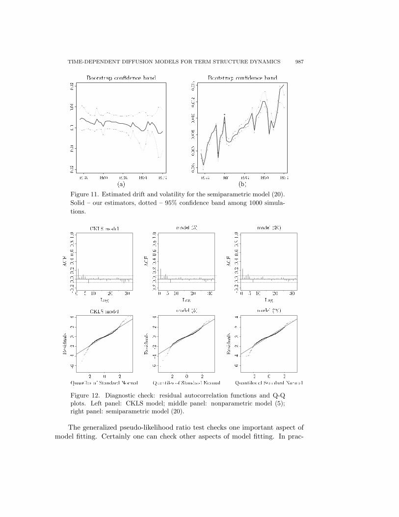
Figure 11. Estimated drift and volatility for the semiparametric model (20).Solid – our estimators, dotted – 95% confidence band among 1000 simula-tions.

Figure 12. Diagnostic check: residual autocorrelation functions and Q-Qplots. Left panel: CKLS model; middle panel: nonparametric model (5);right panel: semiparametric model (20).

The generalized pseudo-likelihood ratio test checks one important aspect ofmodel fitting. Certainly one can check other aspects of model fitting. In prac-


tice, one may also examine if the residuals behave like a Gaussian white noise.To compare the performances of the CKLS model, model (5) and model (20),we consider again the treasury bill data in Section 3.1. (For this set of data,the P -value for testing homogeneity in volatility under model (20) is 0.03.) Theadequacy of the three models can also be assessed by their residual autocorre-lation functions. Figure 12 gives the residual autocorrelation functions and theQ-Q plots for the residuals from the three models. It is evident that, from theQ-Q plots, our models (5) and (20) are more adequate than the CKLS model.Figure 13 reports the estimates of the coefficients in model (20) along with the95% bootstrap confidence bands using 1000 simulations. The estimates of theexpected return and volatility are shown in Figure 14. It seems that the timevariation in volatility occurs after 1980 (admittedly the confidence interval iswide) and not before; this observation is similar to that made in Section 3.1.

Figure 13. Three month treasury Bill rate, from January 2, 1970 to Decem-ber 26, 1997: Estimated coefficient functions for the semiparametric model(20). Solid – our estimators, dash-dotted – 95% confidence band among 1000simulations.

The sample skewness and kurtosis of the original series {Yti} and the residu-als from the three models are reported in Table 6. The kurtoses of the residualsfrom the three models are much smaller in magnitude than that of {Yti}, whichreflects that the three models successfully reveal the phenomena of time-varyingvolatilities in the yields of the treasury bill. Note that the residuals from ourmodel (20) have the smallest kurtosis in this example.


Figure 14. Three month treasury Bill rate, from January 2, 1970 to Decem-ber 26, 1997: Estimated drift and volatility for the semiparametric model(20). Solid – our estimators, dash-dotted – 95% confidence band.

Table 6. Skewness and kurtosis.

Model Skewness Kurtosis

Original series {Yti} -0.002 13.975

Residuals from CKLS model 0.021 4.620

Residuals from Model (5) 0.015 4.429

Residuals from Model (20) 0.009 3.973

7. Conclusion

The time-varying coefficient model (5) is introduced to better capture thetime variation of short-term dynamics. It has been demonstrated to be an ef-fective tool for modelling volatility and validating existing models. It arisesnaturally from various considerations and encompasses most of the commonlyused models as special cases. Yet, due to limited independent data information,coefficients in model (5) may not be estimated very reliably. The semiparametricmodel (20) provides a useful alternative.

Acknowledgements

Fan’s work was partially supported by the NSF Grant DMS-0204329, thegrant CUHK 4299/00 of the Research Grant Council grant of Hong Kong anda direct grant from the Chinese University of Hong Kong. Jiang’s research wassupported in part by Chinese NSF Grants 10001004 and 79800017. Research


of the third author was supported by Wisconsin Alumni Research Foundation.The authors wish to thank the guest Editor, Ruey Tsay, and two anonymousreferees for their constructive comments which improved the presentation of thispaper. We also gratefully acknowledge helpful comments and suggestions fromProfessors Ron Gallant and Jia He.

References

Aıt-Sahalia, Y. (1996a). Nonparametric pricing of interest rate derivative securities. Economet-

rica 64, 527-560.

Aıt-Sahalia, Y. (1996b). Testing continuous-time models of the spot interest rate. Rev. Finan.

Stud. 9, 385-426.

Aıt-Sahalia, Y. and Lo, A. W. (1998). Nonparametric estimation of state-price densities implicit

in financial asset prices. J. Finance 53, 499-548.

Aıt-Sahalia, Y. (1999). Transition densities for interest rate and other nonlinear diffusions. J.

Finance LIV, 1361-1395.

Aıt-Sahalia, Y. (2002). Maximum likelihood estimation of discretely sampled diffusions: A

closed-form approximation approach. Econometrica 70, 223-262.

Andersen, T. G. and Lund, J. (1997). Estimating continuous time stochastic volatility models

of the short-term interest rate. J. Econometrics 77, 343-377.

Black, F., Derman, E. and Toy, W. (1990). A one-factor model of interest rates and its appli-

cation to treasury bond options. Finan. Analysts’ J. 46, 33-39.

Black, F. and Karasinski, P. (1991). Bond and option pricing when short rates are lognormal.

Finan. Analysts’ J. 47, 52-59.

Black, F. and Scholes, M. (1973). The pricing of options and corporate liabilities. J. Polit.

Economy 81, 637-654.

Brennan, M. J. and Schwartz, E. S. (1979). A continuous time approach to the pricing of bonds.

J. Banking Finance 3, 133-155.

Brennan, M. J. and Schwartz, E. S. (1982). An equilibrium model of bond pricing and a test

of market efficiency. J. Finan. Quant. Anal. 17, 210-239.

Buhlman, P. and Kunsch, H. R. (1995). The blockwise bootstrap for general parameters of a

stationary time series. Scand. J. Statist. 22, 35-54.

Chan, K. C., Karolyi, A. G., Longstaff, F. A. and Sanders, A. B. (1992). An empirical compar-

ison of alternative models of the short-term interest rate. J. Finance 47, 1209-1227.

Chapman, D. A. and Pearson, N. D. (2000). Is the short rate drift actually nonlinear? J.

Finance 55, 355-388.

Constantinides, G. M. and Ingersoll, J. E. (1984). Optimal bond trading with personal taxes.

J. Finan. Econom. 13, 299-335.

Cox, J. C., Ingersoll, J. E. and Ross, S. A. (1980). An analysis of variable rate loan contracts.

J. Finance 35, 389-403.

Cox, J. C., Ingersoll, J. E. and Ross, S. A. (1985). A theory of the term structure of interest

rates. Econometrica 53, 385-467.

Dothan, U. L. (1978). On the term structure of interest rates. J. Finan. Econom. 6, 59-69.

Duffie, D. (1996). Dynamic Asset Pricing Theory. 2nd edition. Princeton University Press,

Princeton, New Jersey.

Epanechnikov, V. A. (1969). Nonparametric estimation of a multidimensional probability den-

sity. Theory Probab. Appl. 13, 153-158.


Fan, J. (1993). Local linear regression smoothers and their minimax efficiencies. Ann. Statist.

21, 196-216.

Fan, J. and Gijbels, I. (1995). Data-driven Bandwidth selection in local polynomial fitting:

variable bandwidth and spatial adaptation. J. Roy. Statist. Soc. Ser. B 57, 371-394.

Fan, J. and Gijbels, I. (1996). Local Polynomial Modelling and Its Applications. Chapman and

Hall, London.

Fan, J. and Yao, Q. W. (1998). Efficient estimation of conditional variance functions in stochas-

tic regression. Biometrika 85, 645-660.

Fan, J., Zhang, C. M. and Zhang, J. (2001). Generalized likelihood ratio statistics and Wilks

phenomenon. Ann. Statist. 29, 153-193.

Fan, J. and Zhang, C. M. (2003). A re-examination of Stantan’s diffusion estimators with

applications to financial model validation. J. Amer. Statist. Assoc. 98, 118-134.

Feldman, D. (1989). The term structure of interest rates in a partially observable economy. J.

Finance 44, 789-812.

Florens-Zmirou, D. (1993). On estimating the diffusion coefficient from discrete observations.

J. Appl. Probab. 30, 790-804.

Franke, J., Kreiss, J.-P. and Mammen, E. (2002). Bootstrap of kernel smoothing in nonlinear

time series. Bernoulli 8, 1-37.

Gallant, A. R. and Long, J. R. (1997). Estimating stochastic differential equations efficiently

by minimum chi-squared. Biometrika 84, 125-141.

Gallant, A. R., Rossi, P. E. and Tauchen, G. (1997). Nonlinear dynamic structures. Economet-

rica 61, 871-907.

Gallant, A. R. and Tauchen, G. (1997). Estimation of continuous time models for stock returns

and interest rates. Macroecon. Dynam. 1, 135-168.

Gallant, A. R. and Tauchen, G. (1998). Reprojecting partially observed systems with applica-

tion to interest rate diffusions. J. Amer. Statist. Assoc. 93, 10-24.

Genon-Catalot, V. and Jacod, J. (1993). On the estimation of the diffusion coefficient for

multi-dimensional diffusion processes. Ann. Inst. H. Poincar Probab. Statist. 29, 119-51.

Green, P. J. and Silverman, B. W. (1994). Nonparametric Regression and Generalized Linear

Models: a Roughness Penalty Approach. Chapman and Hall, London.

Hansen, L. P. (1982). Large sample properties of generalized method of moments estimators.

Econometrica 50, 1029-1054.

Hansen, L. P. and Scheinkman, J. A. (1995). Back to the future: generating moment implica-

tions for continuous-time Markov processes. Econometrica 63, 767-804.

Hart, J. D. (1994). Automated kernel smoothing of dependent data by using time series cross-

validation. J. Roy. Statist. Soc. Ser. B 56, 529–542.

Hart, J. D. (1996). Some automated methods of smoothing time-dependent data. J. Non-

parametr. Statist. 2-3, 115-142.

Hardle, W. (1990). Applied Nonparametric Regression. Cambridge University Press, Boston.

Hastie, T. J. and Tibshirani, R. (1990). Generalized Additive Models. Chapman and Hall,

London.

Hastie, T. J. and Loaders, C. (1993). Local regression: automatic kernel carpentry (with

discussion). Statist. Sci. 8, 120-143.

Ho, T. S. Y. and Lee, S. B. (1986). Term structure movements and pricing interest rate

contingent claims. J. Finance 41, 1011-1029.

Hull, J. and White, A. (1990). Pricing interest-rate derivative securities. Rev. Finan. Stud. 3,

573-592.

Hull, J. C. (1997). Options, Futures and Other Derivatives. 3rd edition. Prentice Hall, Upper

Saddle River, New Jersey.


Kunsch, H. R. (1989). The jackknife and the bootstrap for general stationary observations.Ann. Statist. 17, 1217-1241.

Longstaff, F. A. (1989). A nonlinear general equilibrium model of the term structure of interestrates. J. Finan. Econom. 23, 195-224.

Longstaff, F. A. and Schwartz, E. S. (1992). Interest-rate volatility and the term structure: atwo-factor general equilibrium model. J. Finance 47, 1259-1282.

Merton, R. C. (1973). Theory of rational option pricing. Bell J. Econom. Management Sci. 4,141-183.

Merton, R. C. (1992). Continuous-Time Finance. Blackwell, Cambridge, Massachusetts.Mishkin, F. S. (1997). The Economics for Money, Banking and Financial Markets. 5th edition.

Addison-Wesley, New York.Morgan, J. P. (1996). RiskMetrics Technical Document. 4th edition. New York.Ruppert, D. and Wand, M. P. (1994). Multivariate weighted least squares regression. Ann.

Statist. 22, 1346-1370.Ruppert, D., Sheather, S. J. and Wand, M. P. (1995). An effective bandwidth selector for local

least squares regression. J. Amer. Statist. Assoc. 90, 1257-1270.Sandmann, K. and Sondermann, D. (1997). A note on the stability of lognormal interest rate

models and the pricing of Eurodollar futures. Math. Finance 7, 119-125.Scott, D. W. (1992). Multivariate Density Estimation: Theory, Practice and Visualization.

John Wiley, New York.Schaefer, S. and Schwartz, E. (1984). A two-factor model of the term structure: an approximate

analytical solution. J. Finan. Quantitative Anal. 19, 413-424.Simonoff, J. S. (1996). Smoothing Methods in Statistics. Springer-Verlag, New York.Stanton, R. (1997). A nonparametric models of term structure dynamics and the market price

of interest rate risk. J. Finance 52, 1973-2002.Stone, M. (1974). Cross-validatory choice and assessment of statistical predictions (with dis-

cussion). J. Roy. Statist. Soc. Ser. B 36, 111-147.Stutzer, M. (1996). A simple nonparametric approach to derivative security valuation. J.

Finance 51, 1633-1652.Wahba, G. (1977). A survey of some smoothing problems and the method of generalized cross-

validation for solving them. In Applications of Statistics (Edited by P. R. Krisnaiah),507-523. North Holland, Amsterdam.

Vasicek, O. (1977). An equilibrium characterization of the term structure. J. Finan. Econom.5, 177-188.

Wong, E. (1971). Stochastic Processes in Information and Dynamical Systems. McGraw-Hill,New York.

Department of Statistics, Chinese University of Hong Kong, Shatin, Hong Kong.

E-mail: [email protected]

Department of Probability and Statistics, Peking University, Beijing, 100871, P.R.C.


Department of Statistics, University of Wisconsin Madison, WI 53706, U.S.A.


Department of Statistics, University of California Los Angeles, CA 90095, U.S.A.


(Received March 2001; accepted July 2003)

Date post:	18-Apr-2018
Category:	Documents
Upload:	hatu
View:	219 times
Download:	3 times

TIME-DEPENDENT DIFFUSION MODELS FOR TERM STRUCTURE...

Documents