Faculty of Physics and Astronomy, Friedrich-Schiller-University, ena, 6900 Jena, Germany
Received June 16, 1989; revised manuscript received October 31, 1990; accepted November 1, 1990
Matter interacting with light is considered as a linear optical system that may be time-shift invariant or time-shiftvariant, which is important for an ultrashort time technique. The light may be coherent or partially coherent insecond order with respect to time. It is described by the Page distribution. The optical system is characterized by atime-dependent system spectrum, which is adapted to the Page distribution of the light interacting with the systemsand which is related to the optical transfer functions of the system. With the system spectrum and the spectraderived from it, various linear optical systems (spectral instruments without or in connection with shutters, glassslabs, and molecular systems investigated by excitation and probe spectroscopy) are described.
1. INTRODUCTION
Since laser-pulse technology has advanced to the femto-second domain",2 the investigation of nonstationary opticalradiation with the help of optical systems and the study ofshort-time processes play an increasing role. Gratings hadbeen used for pulse compressions and pulse coding.",4 Moregenerally, the interaction of light with time-invariant linearoptical systems, such as optical pupils, gratings, and prismspectrometers,5-9 and the Fabry-Perot interferometer'0
have been analyzed, whereby the systems can be describedby the time-impulse response.
On the level of electric field strength the light can bedescribed by the complex analytical signal" or by the ampli-tude spectrum that is its Fourier transform. For the analy-sis of nonstationary signals there exist various methods thatgo beyond Fourier analysis.'2 One of them is the so-calledrunning Fourier transform,'3 which depends on frequencyand real time. It is a causal function, which means that itdescribes what happens now and "is independent of whatthe signal may do in the future." 13 Another tool for analyz-ing nonstationary signals is the wavelet transform. 1 21 415
Optical radiation is dealt with classically. The light maybe represented by signals in a stochastic or deterministiccontext. In both cases the radiation can be analyzed withthe help of the above methods. Stochastic processes can bedescribed adequately by correlation methods, for instance,by second-order correlation functions. If the second-ordercorrelation function is factorable16 the radiation is said to becoherent in second order. In this case the electric fieldstrength itself can be obtained from the correlation function.Coherent radiation can be approximated by proper lasers,whereas with other lasers or thermal sources the light is moreor less partially coherent with respect to time. It must bementioned that the relations among the correlation func-tions have the same view in classical and quantum theory;the average is performed in another way, however.
Well adapted to the measurement of partially coherentoptical radiation are time-frequency distributions. In thispaper the causal Page distribution is preferred.12"13 Thisdistribution belongs to Cohen's class.12",718 Another mem-ber of this class is the Wigner distribution.' 9 The relationbetween the so-called time-dependent physical spectrum of
light 0 and the Page distributions and the Wigner distribu-tion20 have been investigated. In this paper linear systemswithout quantum fluctuations will be investigated; thus, forinstance, light scattering is not taken into account. Thatmeans that the system can be considered in a deterministiccontext. In an extension of the conventional treatment theoptical systems may be time-shift variant. Molecular sys-tems or semiconductors investigated by means of excitationand probe spectroscopy,2 for instance, can be considered aslinear time-shift-variant optical systems, if, besides theprobing light, there exists an exciting laser pulse thatchanges one or more parameters of the system temporally.Thus the optical system is fully determined by the time-pulse response that depends on a temporal coordinate relat-ed to the memory of the system and on real time t. This is acomplex function (amplitude and phase) depending on twovariables.
For a determination of the properties of the system, theinteraction of light with the systems will be investigated byanalyzing the relation between the input radiation and theoutput radiation after interaction with the optical system.The Page distributions of the input and output radiation areconnected by a functional of the time-impulse response, afunctional that is here called the general system spectrum(GSS). The GSS for time-shift-variant systems will be areal function of two temporal and of two frequency coordi-nates. The GSS contains as much information as the time-impulse response. The advantage will be that the GSS ismore adapted to measurements by square-law detectors,especially to time-resolved measurements in connectionwith a spectrometer and a streak camera 8 21 (spectrochro-nography).
The goal of the present paper is to study the propertiesand usefulness of the time-dependent GSS. For varioustime-shift-variant and time-shift-invariant systems the GSSwill be represented graphically in order to reveal some of itsfeatures. The following results are desired:
(1) The GSS describes in a simple way the evolution ofthe Page distribution of radiation passing through linearoptical systems; thus the properties of nonstationary andpartially coherent radiation can be analyzed.
(2) By investigation of the input and output radiation,the GSS can be determined; thus the properties of linearoptical systems can be analyzed.
(3) Special spectra of time-shift-variant and time-shift-invariant systems, well known in optics, can be derived fromthe GSS. Thus a classification of various system spectra ispossible.
The above methods related to time coordinates are analo-gous to the treatment of quasi-monochromatic radiation,partially coherent with respect to spatial coordinates.2 2
The time-frequency Page distribution corresponds to thespace-angle Wigner distribution (Wolf function 2 3), and theGSS corresponds to the beam spread function,24 a functionof two spatial and two angular coordinates. There exist atleast two essential differences between time and space do-mains. First, in the time domain the time-frequency distri-bution should be causal, whereas, according to spatial coor-dinates perpendicular to the direction of propagation, nocausal function is necessary. Second, in the space domainthe transition from the field strength level to the correlationlevel establishes the generalized ray concept,23' 24 whereas inthe time domain an analogous concept does not seem toexist.
The GSS may have a complicated dependence on thevariables, but, with existing computers, no problems arise inevaluating the results.
Throughout the paper the following agreements will bevalid:
(1) If the integration is carried out from-X to +c, theintegration limits are omitted.
(2) A tilde over a variable of a function means that thefunction does not depend on this variable.
(3) One or two bars over a function means that thisfunction has been integrated once or twice.
2. PROPERTIES OF THE PAGE DISTRIBUTIONIN OPTICS
In this section the properties of the time-frequency Pagedistribution will be summarized. The running Fouriertransform of the electric field strength of the radiation isgiven by' 3
I.t
A(+)(w; t) = J drE(+)(T)exp(-iwr). (1)
Here E(+)(t) and E()(t) are, respectively, the positive andnegative parts of the complex analytical signal1""16 withE(t) = [E(+)(t)]*. Introducing the unit step function
e(x) = {(x S 0)
(x > 0)
and the function
g(x) = 0(-x)exp(-ix), (3)
we can rewrite Eq. (1) in a form resembling the wavelettransformation:
whereas wavelets represent waves of finite length, g(x) de-scribes a one-sided infinitely long wave. On the other hand,the running Fourier transform is a causal function in thesense of Ref. 13, whereas the wavelet transform14 in generalis no causal function.
Now we address the description of the level of correlationfunctions. The correlation function will be represented inthe form16
(5)
where the angle brackets denote an ensemble average. Forthe special case of radiation coherent in second order, thefields strength can be recovered from the correlation func-tion up to a constant phase:
(6)
Here to is an arbitrarily fixed time to < t.Besides thermal radiation, an example of partially coher-
ent nonstationary radiation may be a train of ultrashortpulses8 whose amplitude and phase dependence from timeare changed from pulse to pulse because of statistical fluctu-ations of the resonator properties. As an ensemble, theentire range of pulses is considered.
The Page distribution PE(w, t) is given in the form12"13
PE(w, t) = K a (IAd+)(w; t)12),at
(7)
which, in connection with the Wiener-Khintchine theo-rem,25 26 can also be written as
PE(w, t) = K J drr[t + rO(-T), t + 7r(-r) - T]exp(-iwr).
(8)
The constant K is given by K = A(eo/Mo)/2, where A is thebeam cross-sectional area.
From this formulation with the unit step functions, theinverse formula easily can be obtained:
As is known, the Page distribution has the following proper-ties:
(1) The Page distribution has the dimension of an ener-gy, it is a real function that can take on positive and negativevalues, and it is a causal12 function. In the frame of rotatingwave approximations the Page distribution becomes zero fornegative frequencies.
(2) For the special case of coherent radiation and fromthe Page distribution by means of Eqs. (9) and (6), theelectric field strength can be obtained, in principle.
(3) The Page distribution describes a frequency distri-bution for each real time t. An uncertainty relation thatdepends on time t is valid in the form
[(w - ) t2 (r-r)t2]1/2 > 1/2. (10)
A(+)(W; t)exp(-iwt) = f drE(+)(r)g[(r - t)w. (4)
The function g(x) formally has the view of a wavelet,14 but,
The one and two bars over the symbols indicate formation ofthe first-order and second-order moments, respectively, re-lated to real time t. The moment , is the mean conditional
Rolf Gase
r(tj, t2) = (E(+)(tj)E(-)(t2))1
E(+)(t = [r(t, t)il/2r(t, to)/Ir(t, to)j.
852 J. Opt. Soc. Am. A/Vol. 8, No. 6/June 1991
frequency.18 For coherent radiation an instantaneous fre-quency can be introduced.'8
(4) The energy spectrum 13(w) and the instantaneouspower (t) can be obtained from the Page distribution bythe marginals
G(c) = I dtPE(co, t), (1
(t) = J dWPE(w, t). (12)
These two functions contain only positive values, and theycan be measured by a grating spectrometer with sufficientfrequency resolution and by a detector with sufficient timeresolution, respectively, for Eqs. (11) and (12).
(5) For stationary radiation (which means that the Pagedistribution does not depend on real time t at all) the Pagedistribution equals the Wiener-Khintchine power spec-trum.25 26 In this case the energy spectrum [Eq. (11)] is notdefined.
3. TIME-DEPENDENT SYSTEM SPECTRA
The time impulse response H(+)(r, t) for time-shift-variantsystems is defined by the relationship between input andoutput radiation:
Eout( )(t) = J drH(+)(r, t)Ei(+(t -). (13)
The temporal variable of the time impulse response isrelated to the dynamical behavior of the system. Only fortime-shift-variant systems does the impulse response de-pend on real time t. Since the optical systems shall becausal, H(+)(.r, t) must vanish for r < 0.
The GSS can be calculated from the relation betweeninput and output radiation, whereby the radiation is de-scribed by the Page distribution (see Appendix A):
PEout(@, t) = (1/27r) J dw' J do
X G(w', , W, t)PE in(l', t - ), (14)
with the abbreviation
G(co', 9, a, t) = [ dT A dT r(t, t; to + T' -T t - T)
+ J dT J dT r(, t; t + r' - T t - T)
J JO
+ r dTJ d T rG(9-T ', t; o t - T)].
X exp[i(W'r' - T)] + C.C. (15)
The connection between the input and output Page distribu-tions is similar to a twofold convolution. The kernel G(w', O,co, t) in a general, nonspecified form for all members ofCohen's class is represented by Eq. (7.5) of Ref. 18. Thefunction G(w', , co, t) is the desired time-dependent GSS.The product function
rG(T', t; T", t) = H()(T', t)H(-)(T, t),
appearing in Eq. (15), contains the same information as thetime response itself. The time response can be obtainedfrom the product function analogously to Eq. (6).
The GSS reveals the following properties:
(1) The GSS is a dimensionless real function of two fre-quencies and of two time coordinates, and it can take onpositive and negative values.
(2) Because of memory effects of the system, the outputradiation is smeared over the temporal variable . Fortime-shift-variant systems, additionally optical frequenciescharacterized by w' are generated, which are not contained inthe input radiation.
(3) For time-shift-invariant systems, the GSS does notdepend on real time t, but it still depends on two frequencyvariables X and co'. For the special case of an extremelynarrow bandpath filter with frequency wo, the GSS goes overto 6(W' - co)(w - o), where a means the Dirac function,and, for free space, the GSS takes the form 6(c' - ).
We come to relations simpler than Eq. (14), if we are inter-ested only in the instantaneous power 3(%t) or the energy (e ofthe output radiation. For the output power we obtain fromEq. (14), by integration with respect to a,
Besides the sign of r, the dynamical system spectrum has theform of a Page distribution with respect to the time impulseresponse H(+)(T, t).
We obtain the output energy out by integration of Eq.(17) with respect to time. We arrive at simple relations ifthe system is time-shift invariant:
Bout = (1/2X) dco'G(co')Zin(o')
where the function
GI(o') = J | d J coG(w', t), co, t)
(20)
(21)
is the frequency profile function.9 This function is relatedto the time-impulse response by the simple relation
G1(,') = IR(co)j2, (22)
where the optical transfer function 1t(w') is the Fouriertransform of the time impulse response.
For spectrometers 01(c') is related to the so-called in-strumental function, and for molecules and solids G1(w') isidentical with the transmission or reflection spectrum.
Rolf Gase
(16)
Vol. 8, No. 6/June 1991/J. Opt. Soc. Am. A 853
4. EXAMPLES FOR DYNAMICAL SYSTEMSPECTRA OF TIME-INVARIANT SYSTEMS
A. SpectrometerSpectrometers are time-shift-invariant systems. For vari-ous setting frequencies w, the output power 30out(t; ws) ismeasured in dependence on real time t and on setting fre-quency ws (spectrochronography). The function 3,Jt; s)
is identical with the time-dependent physical spectrum.910
With the help of the coordinate transformtion w' = , -SI
we attain at the dynamical instrumental function of thespectrometer a function of setting frequency w,:
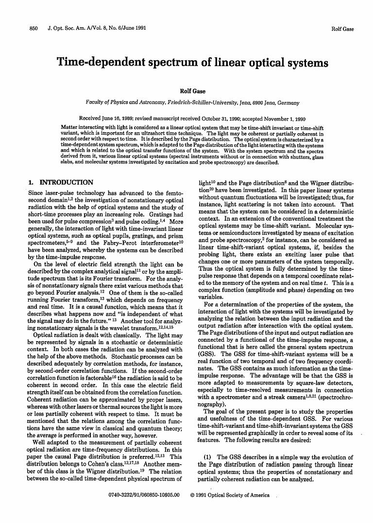
with the help of contour lines. One can see that the tempo-ral width of this function has a value AT = T and thespectral width a value Aw = 2/T. Thus, measuring thetime-dependent physical spectrum of light has smoothedthe Page distribution in frequency and in time with amountsAw and AT, respectively. If we investigate light pulses bymeans of a grating spectrometer with the maximum traveltime T, greater than the pulse length Tp, then Eq. (24) takeson the simple form 8 (see Appendix B, text following Eq.(B8)] of
out(t; ,W) = (/T 2) J d0PEjin(W8, t -), (27)
(23)
According to Eq. (17), we find a relation between the Pagedistribution and the physical spectrum (see Appendix B):
out(t; ws) = (1/2ir) J dQ J do
X D(0, t; Ws)PEin((WS - Q, t - 3). (24)
Here 2B means the bandwidth of the radiation that mayextend over all the optical range. For a grating or prismspectrometer with a sufficiently small slit width, one obtains
D(Q, t); w)
[T" - )/T 2 ]sinc[Q(T - o)] (0 < a < Ts)
t0 (else)
(sinc x means sin xix).The maximum travel time difference T, is related to the
resolving power St by
Ts = 27r9/lw,. (26)
In Fig. 1 the dynamical instrumental function is represented
Q.As
2X
0-
-2X -
/ /
usable for times tm - Tp/2 < t < tm, where tm designates themiddle of the pulse. Equation (27) can be written in theequivalent form
l t$.Ut(t; WUs) = (/T,2) dt"'Ejin(Ws, t ) (28)
Now we see that under the above conditions the Page distri-bution can be inferred from the time-dependent physicalspectrum by means of the inverse relation
PEin(sS t) = T82 at IO3t(t; Ws). (29)
Moreover, for coherent radiation the field strength can bemeasured in principle. An experimentally important resultis that Eq. (24), considered an integral equation, has such asimple solution.
In Section 6, for time-shift-invariant systems the resultsobtained with the Page distribution are compared with thoseobtained with other (noncausal) distributions of Cohen'sclass. Such simple relations as Eq. (28) and (29) can beobtained only with the causal Page distribution.
By conventional spectrometers without time resolution,the output energy is measured in dependence on the settingfrequency w. For such measurements only the knowledgeof the frequency profile function, which in connection withspectrometers in the literature is called instrumental func-tion, is necessary. Starting from Eq. (25) and taking intoaccount Eq. (21), we find that the instrumental function isgiven by the well-known form
D62; w) = sinc2(QT,/2).I.
i.0a)N
0 0.5 i 9'IT5Fig. 1. Dynamical instrumental function D( , 0; w,) of a gratingspectrometer: >0, solid curve; 0, dotted-dashed curve; <0, dashedcurve.
(30)
B. Passing Through GlassFor optical communication the evolution of pulses by pass-ing through glass fibers is of great importance. 2 7 As anoptical system we consider a glass slab of length L. Forcoherent radiation the problem is well solved2 7 on the level offield strength.
The treatment on the level of correlation will reveal thefollowing advantages:
(1) Partially coherent radiation (for instance ultrashortpulses of fluorescent light) can be addressed.
(2) The somewhat problematic expression of instanta-neous frequency'8 does not appear at all.
In order to calculate the dynamical system spectrum, westart from the impulse-response function for the glass slab inthe form
Rolf Gase
D42, 0; co = 0(co - 9, t�, F),,-
854 J. Opt. Soc. Am. A/Vol. 8, No. 6/June 1991
dco' expfi[tw'r - Lk(w')]I.
The bandwidth of the system is limited to 2B, so that lightwith a maximum bandwidth of 2B can be treated. The wavenumber k(w') is developed into a power series about a fixedfrequency o:
k(w') = ko + ko(')O + (1/2!)k O2MU2 + ... , (32)
with Q = - wo. For the dynamical system spectrum weobtain, from Eq. (18) with the impulse-response functiongiven by Eq. (31),
Further, p(Og)l and 44p(tg)J are the modulus and the phase,respectively, of the function
rBP(tg) = J dQ expti[6gg - Lk O2 U2 - Lko(3 )Q3
-. ...
(35)
Lko(l) is to be interpreted as group travel time related tofrequency o and length L, and tOg is the group time delay.
As an example a slab made of flint glass F3 with lengthL =2 mm at frequency o = 3.1 X 10¹⁵ s-i corresponding to anoscillation period To = 2.0 X 10⁻¹⁵ s and to a wavelength X =610 nm will be considered. The following quantities can becalculated for this glass:
For group traveling time,
Lko(') = 35 X 103 /Wo (11.7 ps).
For dispersion of group traveling time,
Lko(2) = 3.2 X 10³ /WO2 (1.72 fs/nm).
For higher dispersion contributions,
Lko(3) = 1.1 X 10³ /( 003 .
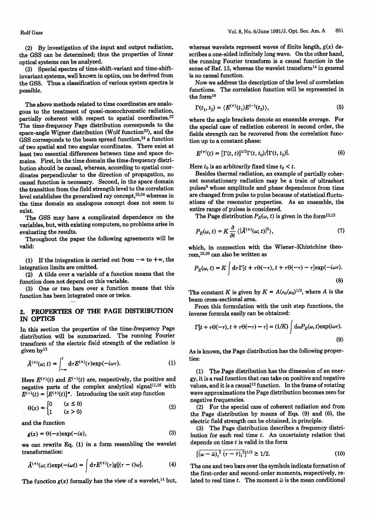
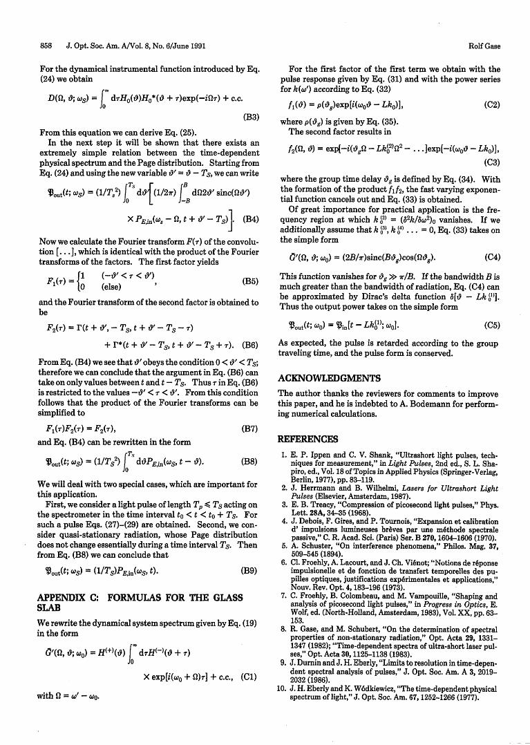
In Fig. 2 the function 0(co', fig) of Eq. (33) for a bandwidth 2B= 0.2wo is represented with the help of contour curves as afunction of (co' - wo)/wo and 13g/To. By using the variable tOg= - Lko(l), we refer to group velocity instead of to phasevelocity.
In Fig. 2 we see in the center a broad mountain ridgeindicated by solid curves; its oblique position is related tothe dispersion of group velocity. Close by, we see narrowravines, the dotted curves indicating the zero level.
We will discuss qualitatively the evolution of the shape ofa short pulse by passing through the glass slab. From Eq.(17) we can conclude that the Page distribution of the inputradiation must be convoluted with the dynamical systemspectrum 0 with respect to the temporal coordinate o, andsubsequently it must be integrated with respect to the spec-tral coordinate w'.
First, let us consider a bandwidth-limited pulse of length25 fs, corresponding to a bandwidth Aw = 0.052 X coo(O.16 X
(31) a
0.05-
0
-0.05-
- - - -e,
--? ,---
-100
Fig. 2. Dynamical systemglass.
0 50 . g/Tospectrum 0C'(0 = '- wo, tOg) for flint
10'5 s-). Regarding Eq. (17), we can estimate from Fig.2 anoutput pulse length of -25To (50 fs).
Second, we consider a chirped pulse of coherent light.The Page distribution of such pulses is characterized by thefact that the mean conditional frequency X is shifted as afunction of time. For instance, for chirped pulses the Pagedistribution is represented in Ref. 28 and the Wigner distri-bution in Ref. 18. One can see immediately that a properlychirped pulse can be shortened by the glass. On the field-strength level, this behavior can be explained by the factthat "different parts of the pulse travel with different groupvelocities." 2
C. Quasi-White RadiationAn example of quasi-white and partially coherent radiationis the fluorescence of molecules after excitation by ultra-short light pulses.' Quasi-white means that the Page distri-bution of light does not change essentially during a frequencyinterval that is given by 6w = l/r, where r, is the correlationtime (memory time) of the system. For quasi-white radia-tion and time-invariant systems Eq. (14) can be approximat-ed by
(36)
Whereas the dynamical system spectrum depends on thevariable o' (the first variable in the GSS), Oq depends on co(the third variable in the GSS) (see Appendix A).
In the treatment of group velocity dispersion related tooptical objectives,2 9 Eq. (36) would be the adequate relation.Further, the Page distribution appearing in Eq. (36) equalsthe time-dependent physical spectrum for quasi-white light[see Eq. (B9) of Appendix B]. Thus the undefined expres-sion intensity as a function of time t and frequency w (orwavelength X) used in Ref. 29 can be replaced by the time-dependent physical spectrum of light.
D. Measurement of the Dynamical System SpectrumOf course, all information on the optical system can be ob-tained by measuring the amplitude and the phase of thefrequency transfer function by means of phase-sensitivemethods, for instance. In this section I will propose a meth-
w+BH+)(r) = (1/27r) |
J w-B
PEout(Wo t) = J dt90q(, W)PEin(W t - 0).
Rolf Gase
-50
Rolf Gase
od to measure the dynamic system spectrum of time-invari-ant systems C(c', ), which may be characterized by thespectral and the temporal bandwidths w'1 and tAl, respective-ly. The testing input radiation shall be a chirp-free square-wave pulse with duration Ts > t9.
To generate such a pulse, we need a nearly chirp-freeultrashort pulse beginning at time to with pulse length Tp <<t)1 and with the mean conditional frequency maximum atthe tunable frequency o. This pulse passes through a grat-ing spectrometer with time constant Ts at frequency coordi-nate s = o. With the dynamical instrumental functionaccording to Eq. (25), the Page distribution of the pulse afterthe spectrometer takes on the form
PE(Co, t; TS)
[30(t - to)2 sinc[( - coo)(t - to)] (0 < t - to < TS)
l0 (else)
(37)
The power of this pulse is $o during 0 < t - to < Ts and zerootherwise.
This square-wave pulse will interact with the system un-der investigation. The output power behind the systemfrom Eq. (17) is obtained to be
The expression { ... is a convolution of two functions. TheFourier transform of this convolution equals the product ofthe Fourier transforms F,(r) and F2(T) of these two func-tions. One can show that under the condition t1 < T, thefunction F2(r) is unity in the region in which F,(r) is differ-ent from zero. Thus Eq. (38) can be rewritten in the simpleform
t-to$out(t; wo) = 0 toT; d6(o, )) (t - to > Ts).
Because Ts > t1, O(co, t) vanishes at the upper integrationlimit. Thus we can replace the upper integration limit by a.Moreover, if we go over to the new variable t + Ts, Eq. (39)results in
This result means that the integral equation [Eq. (17)] bymeans of Eq. (40) can be solved with our square-wave pulse:
0(c 0 , 0) = 09/")Mout(o + to + Ts; coo)/$o
(O < t9<TS). (41)
Summarizing, to measure the dynamic system spectrumO(co', t9) we need a laser to generate tunable ultrashort laserpulses and a spectrochronograph. With the system underinvestigation, between the spectrograph and the detector wemust register the output power during the time interval to +Ts < t < to + Ts + t1 and at tunable frequency oo.
Vol. 8, No. 6/June 1991/J. Opt. Soc. Am. A 855
5. TIME-SHIFT-VARIANT SYSTEMS
A. Quasi-Time-Shift-Invariant SystemsIn excitation and probe spectroscopy2 the sample is probedafter irradiation by a strong excitation pulse at time to withthe help of a weak probe pulse of length Tp and at tunablefrequency cr and variable delay time tin. The probe pulsemay be generated by frequency transformation of a laserpulse or the use of a spectral continuum in connection with amonochromator. (It is important that the light pulse passthe monochromator first and the sample subsequently.) Inthe experiment the output energy gout as a function of comand to is measured. This output energy can be calculatedstarting from Eq. (14) by integration with respect to fre-quency and time.
The molecular systems investigated by excitation andprobe spectroscopy can be considered as quasi-time-shift-invariant systems. These systems are characterized by thecondition that, regarding the response function H(r, t), thecorrelation length r, is much smaller than that time intervalAt during which the response function is nearly constant. Ifadditionally the probe pulse length T p fulfills the condition
(42)r, << Tp << At,
the output energy is given approximately by
yout(WMr tW) = G2 (com, tr)in(con tm)
whereby the function
G2(, t) = 2 J dc' J d6G(c', 6, c, t)
(43)
(44)
will be called the time-resolved system spectrum. [For fullytime-shift-invariant systems, 0 2(, t) is related to the fre-quency profile function G(c') by 0 2(cO, F) = Gj(co' = co).] Bythe simplification leading to Eq. (43), the dispersion of groupvelocity and the generation of new frequencies, of course, arenot taken into account.
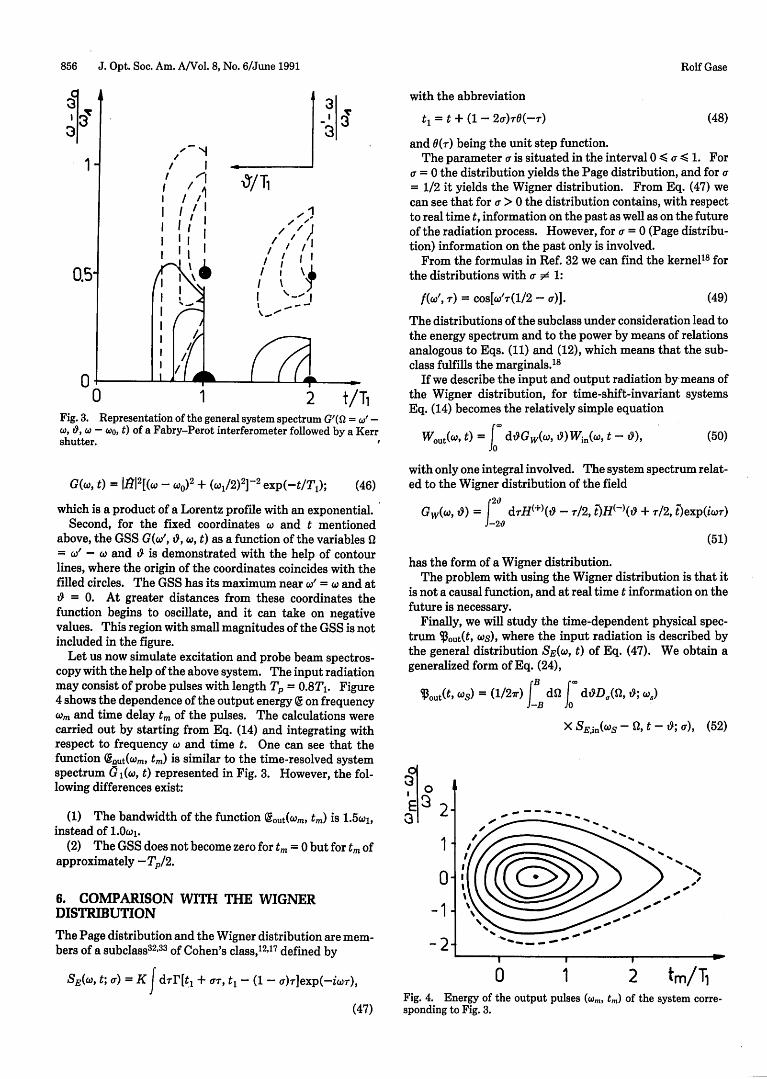
B. Demonstration of a Time-Shift-Variant SystemFor illustration let us deal with a lucid example for a time-shift-variant system, namely, a Fabry-Perot interferometerfollowed by a Kerr shutter.30 The corresponding responsefunction has the form3 l
IP )(,. t) = 1? exp(ioT - cor/2)0(r)exp(-t/2T)0(t)0(T - 0
(45)
(x) being the unit step function. Further, wc is the band-width, co is the setting frequency of the interferometer, andT, characterizes the opening time of the shutter. The GSSof the system under consideration must be used in the gener-al form demonstrated by Eq. (15). This function of fourvariables can be easily written in an explicit form. However,instead of representing this long formula, let us discuss someaspects of the GSS graphically.
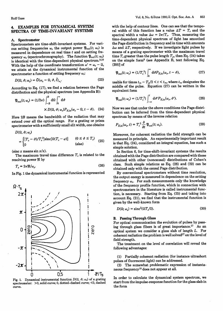
In Fig. 3 a system is considered whose parameters obey thespecial relation coT - 27r. First, for some fixed coordinatesw and t, the values of the time-resolved system spectrumO 2(, t) are indicated by the diameters of the filled circles.This function is zero for t S 0, and for t > 1/1, it takes on theform
856 J. Opt. Soc. Am. A/Vol. 8, No. 6/June 1991
with the abbreviation
t = t + (1 - 20TO(-r)
and 0(r) being the unit step function.The parameter a is situated in the interval 0 < af < 1. For
a = 0 the distribution yields the Page distribution, and for a= 1/2 it yields the Wigner distribution. From Eq. (47) wecan see that for a > 0 the distribution contains, with respectto real time t, information on the past as well as on the futureof the radiation process. However, for aT = 0 (Page distribu-tion) information on the past only is involved.
From the formulas in Ref. 32 we can find the kernel18 forthe distributions with af 1:
f(w', r) = cos[w'r(1/2 - a)].
01 I1 A," I I 1+
o 1 2 t/TFig. 3. Representation of the general system spectrum G'(2 = ' -a, , - coo, t) of a Fabry-Perot interferometer followed by a Kerrshutter. I
The distributions of the subclass under consideration lead tothe energy spectrum and to the power by means of relationsanalogous to Eqs. (11) and (12), which means that the sub-class fulfills the marginals.18
If we describe the input and output radiation by means ofthe Wigner distribution, for time-shift-invariant systemsEq. (14) becomes the relatively simple equation
which is a product of a Lorentz profile with an exponential.Second, for the fixed coordinates and t mentioned
above, the GSS G(w', t, co, t) as a function of the variables Q= co' - co and ) is demonstrated with the help of contourlines, where the origin of the coordinates coincides with thefilled circles. The GSS has its maximum near a' = co and at
= 0. At greater distances from these coordinates thefunction begins to oscillate, and it can take on negativevalues. This region with small magnitudes of the GSS is notincluded in the figure.
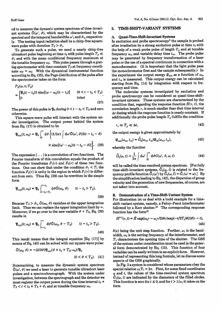
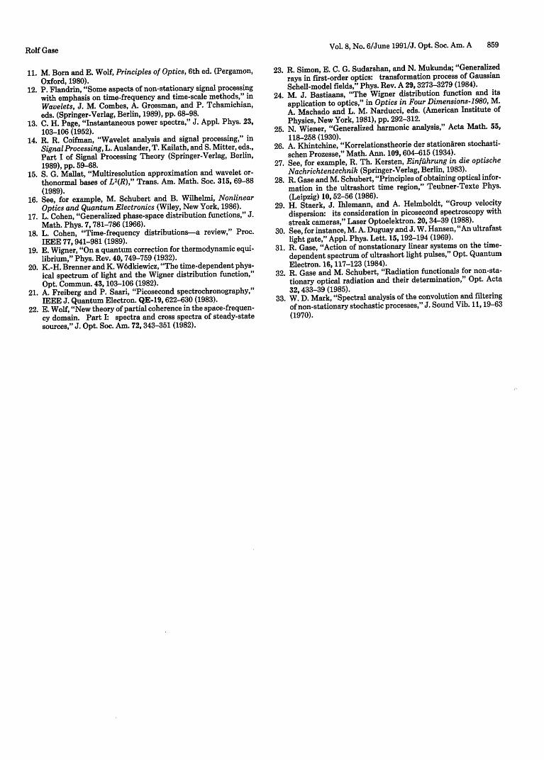
Let us now simulate excitation and probe beam spectros-copy with the help of the above system. The input radiationmay consist of probe pulses with length Tp = 0.8T7. Figure4 shows the dependence of the output energy e on frequencycor and time delay t of the pulses. The calculations werecarried out by starting from Eq. (14) and integrating withrespect to frequency X and time t. One can see that thefunction Lnut(wrn, t) is similar to the time-resolved systemspectrum C (co, t) represented in Fig. 3. However, the fol-lowing differences exist:
(1) The bandwidth of the function Lout(w°, t) is 1.5w1,instead of 1.0w1.
(2) The GSS does not become zero for t = 0 but for t ofapproximately -T p/2.
6. COMPARISON WITH THE WIGNERDISTRIBUTION
The Page distribution and the Wigner distribution are mem-bers of a subclass 32.3 3 of Cohen's class,' 2' 7 defined by
SE(co, t; a) = K J ddr[t + ar, t - (1 - a)T]exp(-ioT),
(47)
with only one integral involved. The system spectrum relat-ed to the Wigner distribution of the field
has the form of a Wigner distribution.The problem with using the Wigner distribution is that it
is not a causal function, and at real time t information on thefuture is necessary.
Finally, we will study the time-dependent physical spec-trum out(t, us), where the input radiation is described bythe general distribution SE(w, t) of Eq. (47). We obtain ageneralized form of Eq. (24),
$ out(tS w) = (1/27r) J dQ J dt9D,(Q, 0; w)B ,
X SEi(s- t - ; a), (52)
0-3 2-
1-
- 1-
) RN
,
0 1
Fig. 4. Energy of the output pulsessponding to Fig. 3.
2 tm/Ti(Wr, t) of the system corre-
Z3^ (48)
(49)
(50)
x | x -
Rolf Gase
__ __ _
Vol. 8, No. 6/June 1991/J. Opt. Soc. Am. A 857
with the generalized dynamical system spectrum
DJ(1, t; ws) = J dTHO(91 - aT; wi)
X Ho* [ 1 + (1 - o)T; wSjexp(-i0T), (53)
with the abbreviation
1= -(1 -2o)rO(-r) (54)
and Ho(); ws) being the window function of the spectrometer[Eq. (Bi) of Appendix B]. The left-hand side of Eq. (53), ofcourse, is independent of a.
For af = 0, Eq. (53) yields Eq. (B3) of Appendix B. For a =1/2 the expressions related to the unit step function vanish.The corresponding relations had been investigated by Bren-ner and W6dkiewicz.20
However, there arise two problems with using the distri-bution with a d 0. First, in order to form the instantaneousoutput power rout, one must know the future of the radiationprocess with respect to real time t. Subsequently, by theconvolution with the dynamical system spectrum, thoseparts of the distribution concerning the future are cut off. Itseems to be more logical to work from the beginning with thedistribution a = 0. Second, if we consider Eq. (52) as anintegral equation for the determination of the unknown dis-tribution SE,in(W, t), with or d 0 such simple relations as thosegiven by Eqs. (27)-(29) are not available. In summary, itcan be said that the Page distribution is well suited to de-scribe the spectral and temporal behavior of the opticalradiation interacting with linear optical systems.
APPENDIX A: DERIVATION OF THEGENERAL SYSTEM SPECTRUM
We start from the output field strength in the form
E(+(t) = J d6H(+)(6, t)Ef!' )(t -),
E(U)(t) = J dr'H(-)( + r'- T, t - r)
X En [t - - ( + 7` - )].
(Al)
(A2)
We rewrite Eq. (8) in the equivalent form,
PE(,w t) = K J drr(t, t - )exp(-iw'r) + c.c., (A3)
and obtain for the Page distribution of the output radiation
PEOUt(,w, t) = K J dTfrJ dt 9 dr'
X G(t6, t; t + r' - t T)
X r(t - , t - - r')exp(-iwT) + c.c. (A4)
The integration region is divided into three parts:
PE',ut(w, t) = (1/2ir) J dw' J dot J dr J dr'
X IrGO(, t; a + T' - 7, t - T)expli(w'r' - -T)] + c.c.)
X PEin(°W t - ), (A5)
1bEout(Ow t) = (1/2ir) J dw' J d)o dr J d' .'..
X PEJJ4 t - )), (A6)
PCEout( = (1/27r) dw' f d o dT I dT'j.
X PE n(W t - - T'). (A7)
By replacing the variable t5 by ) + T', we transform the lastexpression into
PEout t) = (1/2r) J d? oJ dd J dr J dT'
X rG(t - T', t; - T, t - r)exp[i(CO - WT)] + C.Cj
X PEin(& t - ). (A8)
Equations (14) and (15) are obtained by summation of thethree parts of the output distribution.
Let us now derive the dynamical system spectrum fortime-shift-variant systems 0(w', , t) as a function of rG.According to Eq. (15), we obtain for the three regions, (a),(b), and (c),
where Kr) is Dirac's delta function.Summation of both Eqs. (All) and (A12) leads to C(w', ),
t) given by Eq. (19). For quasi-white radiation (see Subsec-tion 4.0) we neglect in Eqs. (A5)-(A7) the dependence on a';thus we obtain for the function Gq(O, W) in Eq. (36)
APPENDIX B: FORMULAS FOR THEGRATING AND PRISM SPECTROMETERS
The window function HO(T) is defined by9
H( )(r, F) = H0(r)exp(iw,,s), (Bi)
and it has the form8
HO(r) = {l/Ts (0 (else) Ts
Rolf Gase
oa(,,.,, 0, t = 0,
(a) > 0; -r > ,(b) 7 < 0; r > ,(c) T < t�; r < ;
(B2)
858 J. Opt. Soc. Am. A/Vol. 8, No. 6/June 1991
For the dynamical instrumental function introduced by Eq.(24) we obtain
D(, 9; s) = d-rH0()H 0*(0 + i)exp(-iQr) + c.c.
(B3)
From this equation we can derive Eq. (25).In the next step it will be shown that there exists an
extremely simple relation between the time-dependentphysical spectrum and the Page distribution. Starting fromEq. (24) and using the new variable tO' = - Ts, we can write
Now we calculate the Fourier transform F(r) of the convolu-tion [... ., which is identical with the product of the Fouriertransforms of the factors. The first factor yields
(else)
and the Fourier transform of the second factor is obtainbe
F2(T) = r(t + , -Ts, t + 6'-Ts - 7)
For the first factor of the first term we obtain with thepulse response given by Eq. (31) and with the power seriesfor k(w') according to Eq. (32)
f1(O) = p(t)g)exp[i(woO -Lko)] (C2)
where p(Og) is given by Eq. (35).The second factor results in
where the group time delay fig is defined by Eq. (34). Withthe formation of the product flf2, the fast varying exponen-tial function cancels out and Eq. (33) is obtained.
Of great importance for practical application is the fre-quency region at which k (2) = ( 2k/bW2)o vanishes. If weadditionally assume that k k 0 ... = 0, Eq. (33) takes onthe simple form
0'(0, 9; coo) = (2B/7r)sinc(Btng)cos(2tg). (C4)
(B5) This function vanishes for Og >> 7r/B. If the bandwidth B ismuch greater than the bandwidth of radiation, Eq. (C4) canbe approximated by Dirac's delta function 6[ - Lk (1)].
led to Thus the output power takes on the simple form
30ut(t; wo) = -[t - Lkl); cool. (05)
+ r*(t + d- Ts, t + ' -Ts + ). (B6)From Eq. (B4) we see that O' obeys the condition 0 < ' < Ts;therefore we can conclude that the argument in Eq. (B6) cantake on only values between t and t - Ts. Thus r in Eq. (B6)is restricted to the values-)' < r < t'. From this conditionfollows that the product of the Fourier transforms can besimplified to
F1(r)F2 (T) = F2(r) (B7)
and Eq. (B4) can be rewritten in the form
$ 0 t(t; cS) = (1/Ts2 ) J doPEii(cs t ). (B8)
We will deal with two special cases, which are important forthis application.
First, we consider a light pulse of length Tp 4 Ts acting onthe spectrometer in the time interval to < t < to + Ts. Forsuch a pulse Eqs. (27)-(29) are obtained. Second, we con-sider quasi-stationary radiation, whose Page distributiondoes not change essentially during a time interval Ts. Thenfrom Eq. (B8) we can conclude that
$out(t; soS) = (1/Ts)PEJ(cos, t). (B9)
APPENDIX C: FORMULAS FOR THE GLASSSLAB
We rewrite the dynamical system spectrum given by Eq. (19)in the form
0'(9, i0; co) = H(+)(O) | dTH()( + r)
X exp[i(w 0 + )r] + c.c., (Cl)
with 0 = c' - coo.
As expected, the pulse is retarded according to the grouptraveling time, and the pulse form is conserved.
ACKNOWLEDGMENTS
The author thanks the reviewers for comments to improvethis paper, and he is indebted to A. Bodemann for perform-ing numerical calculations.
REFERENCES
1. E. P. Ippen and C. V. Shank, "Ultrashort light pulses, tech-niques for measurement," in Light Pulses, 2nd ed., S. L. Sha-piro, ed., Vol. 18 of Topics in Applied Physics (Springer-Verlag,Berlin, 1977), pp. 83-119.
2. J. Herrmann and B. Wilhelmi, Lasers for Ultrashort LightPulses (Elsevier, Amsterdam, 1987).
3. E. B. Treacy, "Compression of picosecond light pulses," Phys.Lett. 28A, 34-35 (1968).
4. J. Debois, F. Gires, and P. Tournois, "Expansion et calibrationd' impulsions lumineuses braves par une mthode spectralepassive," C. R. Acad. Sci. (Paris) Ser. B 270,1604-1606 (1970).
5. A. Schuster, "On interference phenomena," Philos. Mag, 37,509-545 (1894).
6. Cl. Froehly, A. Lacourt, and J. Ch. Vienot; "Notions de rponseimpulsionelle et de fonction de transfert temporelles des pu-pilles optiques, justifications experimentales et applications,"Nouv. Rev. Opt. 4,183-196 (1973).
7. C. Froehly, B. Colombeau, and M. Vampouille, "Shaping andanalysis of picosecond light pulses," in Progress in Optics, E.Wolf, ed. (North-Holland, Amsterdam, 1983), Vol. XX, pp. 63-153.
8. R. Gase, and M. Schubert, "On the determination of spectralproperties of non-stationary radiation," Opt. Acta 29, 1331-1347 (1982); "Time-dependent spectra of ultra-short laser pul-ses," Opt. Acta 30,1125-1138 (1983).
9. J. Durnin and J. H. Eberly, "Limits to resolution in time-depen-dent spectral analysis of pulses," J. Opt. Soc. Am. A 3, 2019-2032 (1986).
10. J. H. Eberly and K. W6dkiewicz, "The time-dependent physicalspectrum of light," J. Opt. Soc. Am. 67, 1252-1266 (1977).
Rolf Gase
F, (,r = 1to
Rolf Gase
11. M. Born and E. Wolf, Principles of Optics, 6th ed. (Pergamon,Oxford, 1980).
12. P. Flandrin, "Some aspects of non-stationary signal processingwith emphasis on time-frequency and time-scale methods," inWavelets, J. M. Combes, A. Grossman, and P. Tchamichian,eds. (Springer-Verlag, Berlin, 1989), pp. 68-98.
13. C. H. Page, "Instantaneous power spectra," J. Appl. Phys. 23,103-106 (1952).
14. R. R. Coifman, "Wavelet analysis and signal processing," in
Signal Processing, L. Auslander, T. Kailath, and S. Mitter, eds.,Part I of Signal Processing Theory (Springer-Verlag, Berlin,1989), pp. 59-68.
15. S. G. Mallat, "Multiresolution approximation and wavelet or-
(1989).16. See, for example, M. Schubert and B. Wilhelmi, Nonlinear
Optics and Quantum Electronics (Wiley, New York, 1986).17. L. Cohen, "Generalized phase-space distribution functions," J.
Math. Phys. 7, 781-786 (1966).18. L. Cohen, "Time-frequency distributions-a review," Proc.
IEEE 77,941-981 (1989).19. E. Wigner, "On a quantum correction for thermodynamic equi-
librium," Phys. Rev. 40,749-759 (1932).20. K.-H. Brenner and K. W6dkiewicz, "The time-dependent phys-
ical spectrum of light and the Wigner distribution function,"Opt. Commun. 43, 103-106 (1982).
21. A. Freiberg and P. Saari, "Picosecond spectrochronography,"IEEE J. Quantum Electron. QE-19, 622-630 (1983).
22. E. Wolf, "New theory of partial coherence in the space-frequen-cy domain. Part I: spectra and cross spectra of steady-statesources," J. Opt. Soc. Am. 72,343-351 (1982).
Vol. 8, No. 6/June 1991/J. Opt. Soc. Am. A 859
23. R. Simon, E. C. G. Sudarshan, and N. Mukunda; "Generalizedrays in first-order optics: transformation process of GaussianSchell-model fields," Phys. Rev. A 29, 3273-3279 (1984).
24. M. J. Bastiaans, "The Wigner distribution function and itsapplication to optics," in Optics in Four Dimensions-1980, M.A. Machado and L. M. Narducci, eds. (American Institute of
Physics, New York, 1981), pp. 292-312.25. N. Wiener, "Generalized harmonic analysis," Acta Math. 55,
118-258 (1930).26. A. Khintchine, "Korrelationstheorie der stationdren stochasti-
schen Prozesse," Math. Ann. 109, 604-615 (1934).27. See, for example, R. Th. Kersten, Einftzhrung in die optische
Nachrichtentechnik (Springer-Verlag, Berlin, 1983).28. R. Gase and M. Schubert, "Principles of obtaining optical infor-
mation in the ultrashort time region," Teubner-Texte Phys.(Leipzig) 10, 52-56 (1986).
29. H. Staerk, J. Ihlemann, and A. Helmboldt, "Group velocitydispersion: its consideration in picosecond spectroscopy withstreak cameras," Laser Optoelektron. 20, 34-39 (1988).
30. See, for instance, M. A. Duguay and J. W. Hansen, "An ultrafastlight gate," Appl. Phys. Lett. 15, 192-194 (1969).
31. R. Gase, "Action of nonstationary linear systems on the time-dependent spectrum of ultrashort light pulses," Opt. QuantumElectron. 16,117-123 (1984).
32. R. Gase and M. Schubert, "Radiation functionals for non-sta-tionary optical radiation and their determination," Opt. Acta32,433-39 (1985).
33. W. D. Mark, "Spectral analysis of the convolution and filteringof non-stationary stochastic processes," J. Sound Vib. 11, 19-63(1970).