TIME-DOMAINANALYSISOFOPENRESONATORS ... In Electromagnetics Research, PIER 61, 1–26, 2006...

Progress In Electromagnetics Research, PIER 61, 1–26, 2006

TIME-DOMAIN ANALYSIS OF OPEN RESONATORS.ANALYTICAL GROUNDS

L. G. Velychko and Y. K. Sirenko

Institute of Radiophysics and ElectronicsNational Academy of Sciences of Ukraine12 Acad. Proskura St., Kharkov 61085, Ukraine

O. S. Velychko

Kharkov National University4 Svobody Sq., Kharkov 61077, Ukraine

Abstract—The paper is concerned with the development andmathematical justification of the methodology for applying the time-domain methods in the study of spectral characteristics of openelectrodynamic resonant structures.

1. INTRODUCTION

This paper is concerned with the solution of theoretical andmethodological problems arising in the time-domain (TD) analysis ofopen resonators (OR). The potentialities of the frequency-domain (FD)methods as applied to the problems of this kind have been almostexhausted. This became evident when researches came up againstthe synthesis problems for open dispersive structures in resonantquasi-optics, for electrodynamic systems in devices of solid-state orvacuum electronics, and others. The application of more universalTD methods [1, 2] to the analysis of resonance conditions, whichare acutely sensitive to variations in the system parameters, mustbe grounded on stable and reliable numerical algorithms. At thesame time, the physical treatment of the numerical results here isimpossible without justified and simplified analytical representationsfor the solutions of the initial boundary-value problems considered. Innumerical experiments, proper allowance must be made for the results

2 Velychko, Sirenko, and Velychko

obtained in FD. We propose to consider the basic stages of the studyof OR by the example of the transient E-polarized fields in the nearzone of compact inhomogeneities of the R2-space. Similar reasoningholds in the case of H-polarization and in 3-D vector case as well, andfor OR of other types [3].

We discuss the following points:– rigorous formulation and solution of initial boundary-value

problems in the theory of OR (the finite difference method with‘fully absorbing’ conditions on the artificial boundaries of theanalysis domain);

– well-grounded analytical relations between spatial-temporal andspatial-frequency representations for the solutions;

– the problem of choice of the pulsed source in numericalexperiments;

– the general methodology for analyzing OR by TD methods.

2. INITIAL BOUNDARY-VALUE PROBLEMS OF THETHEORY OF OPEN COMPACT RESONATORS

We consider a two-dimensional initial boundary-value problem

P [U ] ≡[−ε(g) ∂

2

∂t2−σ(g) ∂

∂t+∂2

∂y2+∂2

∂z2

]U(g, t) = F (g, t) ≡ ∂Jx

∂t,

g = y, z ∈ Q, t > 0

U(g, t)|g∈S = 0, t ≥ 0

U(g, 0) = ϕ(g),∂U(g, t)∂t

∣∣∣∣t=0

= ψ(g), g ∈ Q

,

(1)describing transient states of E-polarized (∂/∂x ≡ 0, U(g, t) =Ex(g, t), Ey = Ez = Hx = jy = jz = 0, ∂Hy/∂t = −η−1

0 ∂Ex/∂z, and∂Hz/∂t = −η−1

0 ∂Ex/∂y) electromagnetic waves E, H in compactopen resonators, whose geometry (Fig. 1) is specified by the real-valued finite functions ε(g) − 1, σ(g) and by the contours S that arethe boundaries of the domains intS filled with a perfect conductor(Q = R2\intS).

Here g = y, z is a point in R2-space, G is the closure ofthe domain G, E ≡ E(g, t) and H ≡ H(g, t) are the electric andmagnetic field vectors, η0 =

√µ0/ε0 is the free space impedance,

ε0 and µ0 are the electrical and magnetic constants, J = η0j (j ≡j(g, t)) is the extraneous current density, σ = η0σ0, ε ≡ ε(g) ≥ 1

Progress In Electromagnetics Research, PIER 61, 2006 3

SOURCES

y

z1

34

S

y = L y = L

L

z = L 2

sources

z = L1

G

(g), (g)ε σL QL

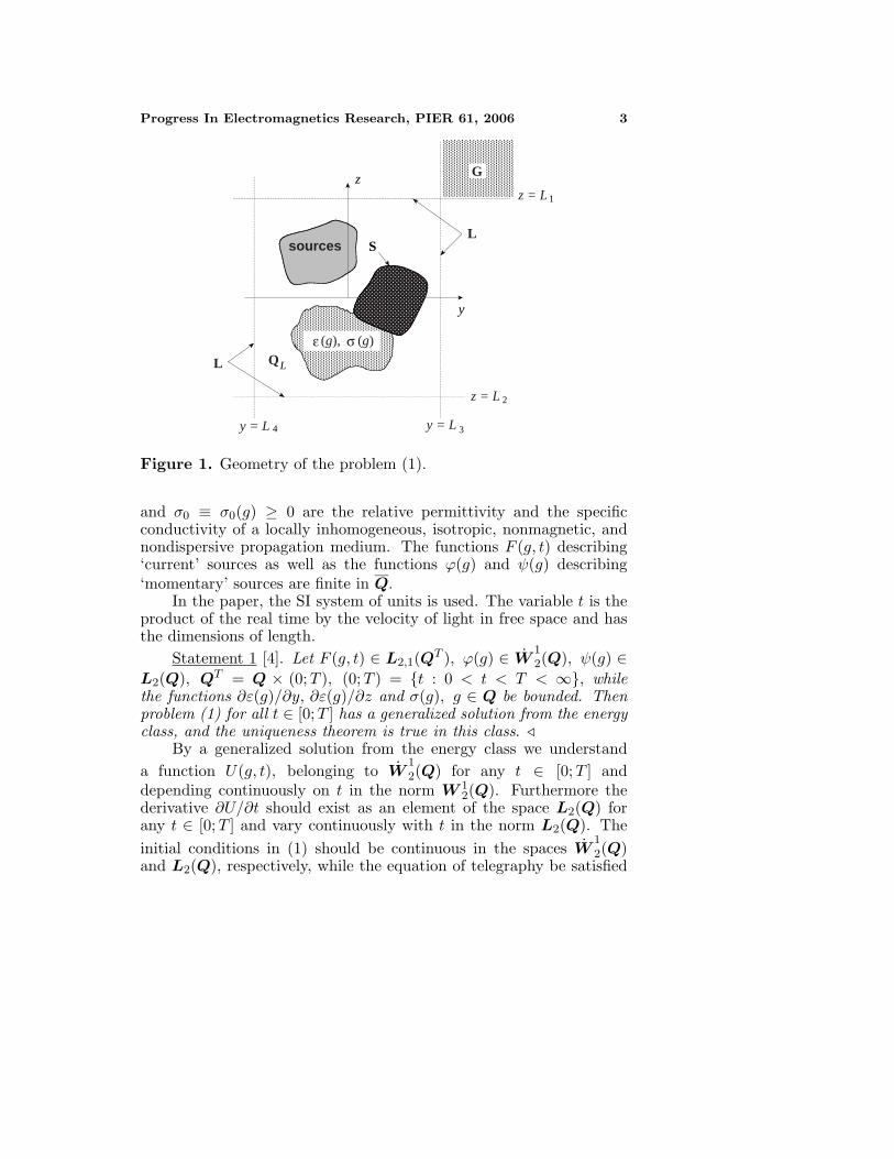
Figure 1. Geometry of the problem (1).

and σ0 ≡ σ0(g) ≥ 0 are the relative permittivity and the specificconductivity of a locally inhomogeneous, isotropic, nonmagnetic, andnondispersive propagation medium. The functions F (g, t) describing‘current’ sources as well as the functions ϕ(g) and ψ(g) describing‘momentary’ sources are finite in Q.

In the paper, the SI system of units is used. The variable t is theproduct of the real time by the velocity of light in free space and hasthe dimensions of length.

Statement 1 [4]. Let F (g, t) ∈ L2,1(QT ), ϕ(g) ∈ W12(Q), ψ(g) ∈

L2(Q), QT = Q × (0;T ), (0;T ) = t : 0 < t < T < ∞, whilethe functions ∂ε(g)/∂y, ∂ε(g)/∂z and σ(g), g ∈ Q be bounded. Thenproblem (1) for all t ∈ [0;T ] has a generalized solution from the energyclass, and the uniqueness theorem is true in this class.

By a generalized solution from the energy class we understanda function U(g, t), belonging to W

12(Q) for any t ∈ [0;T ] and

depending continuously on t in the norm W 12(Q). Furthermore the

derivative ∂U/∂t should exist as an element of the space L2(Q) forany t ∈ [0;T ] and vary continuously with t in the norm L2(Q). Theinitial conditions in (1) should be continuous in the spaces W

12(Q)

and L2(Q), respectively, while the equation of telegraphy be satisfied


in terms of the identity∫QT

ε

(∂

∂tU

)(∂

∂tγ

)−σ

(∂

∂tU

)γ−

(∂

∂yU

)(∂

∂yγ

)−

(∂

∂zU

)(∂

∂zγ

)dgdt

+∫Q

εψγ(g, 0)dg =∫

QT

Fγdgdt.

Here γ = γ(g, t) is an arbitrary element from W 12,0(Q

T ) such thatγ(g, T ) = 0. This identity is derived in a formal way from the followingidentity

(P [U ] − F, γ) =∫

QT

(P [U ] − F )γdgdt = 0

by means of single partial integration of the terms, containing secondorder derivatives of the function U(g, t). In [4] it was proven that sucha definition makes sense and is actually a generalized notion of theclassic solution.

Under practically the same assumptions, the unique solvability ofthe problem (1) and problems (1) with the impedance type boundaryconditions in the space W 1

2(QT ) has been proved in [4]. The

class of generalized solutions, that has been called the energy class,is somewhat narrower than the class of generalized solutions fromW 1

2(QT ). However, it can be proved for this class that the solution

U(g, t) has the same differential features that are assumed satisfied atthe initial time (continuable initial conditions). Besides, for a U(g, t)from this class the following energy relation is satisfied

∫Q

(ε

(∂U

∂t

)2

+|gradU |2)dg

∣∣∣∣∣T

0

+2∫

QT

(σ

(∂U

∂t

)2

+(F∂U

∂t

))dg dt = 0.

(2)

3. FINITE-DIFFERENCE METHOD

The finite difference method reduces problem (1) with σ ≡ 0 and t ∈[0;T ] to determining the mesh functions u = U(yj , zk, tm) = U(j, k,m)that satisfy the difference equations[

−ε(j, k)Dt+D

t− +Dy

+Dy− +Dz

+Dz−

]u = F (j, k,m) (3)

at the mesh points gjk = yj , zk ∈ Q(h, T ) on the time layerstm = ml, m = 0, 1, . . . ,M − 1 = T/l. They are complemented by


the equationsU(j, k, 0) = ϕ(j, k), U(j, k, 1) = ϕ(j, k) + lψ(j, k), gjk ∈ Q(h, T )U(j, k,m) = 0, gjk ∈ S(h, T ), m = 0, 1, . . . ,M − 1

(4)(i.e., the difference analogues of the initial and boundary conditionsin (1)). Here Dy

+[u] = h−1[U(j + 1, k,m) − U(j, k,m)] and Dy−[u] =

h−1[U(j, k,m)−U(j−1, k,m)] are the standard operators of the right-and left-hand difference derivatives (the same with obvious changes istrue also for Dz

±[u], Dt±[u]); yj = jh, zk = kh, j, k = 0,±1, . . . ; h > 0

and l > 0 are the space-step and the time-step of the mesh; all meshfunctions f(j, k) at the mesh points gjk ∈ Q(h, T ) are constructed withrespect to f(g), g ∈ Q as the averages

f(j, k) = h−2∫

ωh(j,k)

f(g)dg,

ωh(j, k) = g : jh < y < (j + 1)h; kh < z < (k + 1)h,

Q(h, T ) is the union of cells ωh(j, k) belonging to Q(T ); S(h, T ) is theboundary of Q(h, T ); Q(T ) is the cut of the cone of influence of sourcesF (g, t), ϕ(g), and ψ(g) in the region Q at the time t = τ > T . It isobvious that equations (3) and (4) uniquely determine u, and u can becalculated without inversion of any matrix operators (i.e., through anexplicit scheme).

The finite-difference scheme is considered to be stable, if for theapproximate solutions u a boundedness can be determined that isuniform with respect to h and l. From the stability, the intrinsicconvergence of the sequence uh,l follows, and the limiting functionu will be the solution to the original initial boundary-value problemprovided that this problem is approximated by finite differenceequations. The latter is satisfied for (1) and for (3), (4). As for thestability of the considered scheme, it is most convenient to analyze itin the ’energy’ spaces where the original problem is well posed. In [4],the validity of the following statement has been proven on the basis ofdifference analogues of the energy inequalities.

Statement 2. Let the functions F (g, t), ϕ(g), ψ(g), and ε(g) − 1that are finite in the region Q be such that F (g, t) ∈ L2,1(QT ), ϕ(g) ∈W 1

2(Q), ψ(g) ∈ L2(Q) and ξ ≤ ε−1(g) ≤ η; g ∈ Q, while thederivatives ∂ε(g)/∂y and ∂ε(g)/∂z are bounded. Then the normsW 1

2(QT ) of the continuous multilinear complements u of solutions u

to problems (3), (4) (the interpolations of the mesh functions u thatare linear in each variable) are uniformly bounded for any h and l that


satisfy one of the following conditions:

η√

2√ξ

l

h< 1 or 2

√ηl

h< 1. (5)

The sequence uh,l converges weakly in W 12(Q

T ) and strongly inL2(QT ) to the solution U(g, t) of the problem (1) as h, l→ 0.

4. TRUNCATION OF THE COMPUTATIONALDOMAIN: “FULLY ABSORBING” CONDITIONS

In Section 3, when describing a general procedure of the algorithmiza-tion of problem (1) by the finite-difference method, we have truncatedthe computational domain by applying the well-known exact radiationcondition

U(g, t)∣∣∣g∈L, t∈[0;T ]

= 0 (6)

for the waves U(g, t) outgoing from the region where the sources andscatterers are localized. The artificial boundary L must be situated,in this case, outside the region G ⊂ Q, whose points are reached bythe excitation U(g, t) by the time t = T . The principal shortcomingof this approach consists in the necessity to extend the computationaldomain with increasing T .

The Absorbing Boundary Conditions (see for example [5–8]) andthe perfectly-matched absorbing layers [9, 10] allow one to ‘close’ openinitial boundary-value problems by the nearby fixed boundaries L, butthey distort the simulated processes to some extent. These distortionsgrow as the observation time t increases [3].

The resonant modes of the nonsinusoidal-wave scattering arehighly sensitive to the influence of the virtual fields caused byreflections from the imperfect ‘absorbing’ boundaries L. Thecalculation of resonance electrodynamic characteristics calls, as a rule,for a long time intervals 0 < t < T [11]. Therefore, the reliable analysisof field oscillations in open high-Q resonant structures must not exploitthose algorithms that truncate the computational domain inefficiently.In the present paper, the problem is solved with the help of the ‘fullyabsorbing’ conditions

[∂

∂t± ∂

∂z

]U(g, t) =

2π

π/2∫0

∂V1(g, t, ϕ)∂t

sin2 ϕdϕ, L4 ≤ y ≤ L3, t ≥ 0,


[∂2V1(g, t, ϕ)

∂t2− ∂

2W1(g, t, ϕ)∂y2

]= 0, L4<y<L3, t>0

∂V1(g, t, ϕ)∂t

∣∣∣∣t=0

= V1(g, t, ϕ)∣∣∣t=0

= 0, L4 < y < L3

;z = L1

z = L2,

(7)[∂

∂t± ∂

∂y

]U(g, t) =

2π

π/2∫0

∂V2(g, t, ϕ)∂t

sin2 ϕdϕ, L2 ≤ y ≤ L1, t ≥ 0,

[∂2V2(g, t, ϕ)

∂t2− ∂

2W2(g, t, ϕ)∂z2

]= 0, L2<y<L1, t>0

∂V2(g, t, ϕ)∂t

∣∣∣∣t=0

= V2(g, t, ϕ)∣∣∣t=0

= 0, L2 < y < L1

;z = L3

z = L4,

(8)

[∂

∂t± cosϕ

∂

∂y

]W1(g, t, ϕ)

=2 cosϕπ

π/2∫0

sin2 γ

cos2 ϕ+ sin2 ϕ cos2 γ∂W2(g, t, γ)

∂tdγ

[∂

∂t± cosϕ

∂

∂z

]W2(g, t, ϕ)

=2 cosϕπ

π/2∫0

sin2 γ

cos2 ϕ+ sin2 ϕ cos2 γ∂W1(g, t, γ)

∂tdγ

, t ≥ 0,

(9)++

→ g = L3, L1,

+−

→ L3, L2,−

+

= L4, L1,

−−

→ L4, L2.

Formulas (7)–(9) represent the exact local ‘absorbing’ condition for theentire artificial coordinate boundary L. In this case, L is the boundaryof the rectangular domain QL = g ∈ Q : L4 < y < L3; L2 < z < L1(Fig. 1) enveloping all sources and compact inhomogeneities of R2-space. Conditions (7)–(9), reducing the analysis domain Q of problem(1) down to QL, have been constructed in [3, 12] without any heuristicassumptions about a fine structure of the field in the vicinity of theartificial boundary. They most closely correspond to the nature ofthe simulated physical processes. The errors introduced by these


conditions are less by an order than the finite-difference approximationerror [3]. Equations (9) play a part of boundary conditions in theauxiliary initial boundary-value problems within formulas (7) and(8). Here Wj(g, t, ϕ) = Vj(g, t, ϕ) cos2 ϕ + U(g, t) (j = 1, 2) and

++

→ g = L3, L1 specifies the signs in the upper and lower

equations for different corner points g = y, z.In essence, formulas (7)–(9) are the analogue of the exact condition

(6) in the domain, where the spatial-temporal transformations of anelectromagnetic field can be arbitrary in intensity. The boundary Ldivides the infinite domain Q of the original problem into two ones,namely, QL and LQ (Q = QL

⋃L Q

⋃L). In the former (bounded)

region, the standard finite-difference algorithms are used for solvingproblem (1) with conditions (7)–(9). In the latter region, the fieldU(g, t) is determined by its values on the boundary L [3, 12].

Statement 3. Problem (1) in the domain Q and problem (1) in thedomain QL = g ∈ Q : L4 < y < L3; L2 < z < L1 with conditions(7)–(9) on its exterior rectangular boundary L are equivalent.

The internal initial boundary-value problems in (7), (8) are wellposed with respect to the auxiliary functionsW1(g, t, ϕ) andW2(g, t, ϕ).

The Statement validity results from the following three facts. Theoriginal problem is uniquely solvable [4]. The solution to the originalproblem is, at the same time, the solution to the modified problem (inconstruction). The solution to the modified problem is unique. Thelast-named fact can be proved by using ‘energy’ estimates for the realfunction U(g, t) (see, for example, [4, 13]).

5. SPACE-TIME REPRESENTATIONS FOR TRANSIENTFIELDS

Based on the ‘energy’ estimates, Statement 1 can be reformulatedin terms of the space W 1

2(Q∞, β) ≡ U(g, t) : U(g, t) exp(−βt) ∈

W 12(Q

∞); β ≥ 0. Hence [4, 14], the direct and inverse Laplacetransforms

f(s) = L[f ](s) ≡∞∫0

f(t)e−stdt↔ f(t) = L−1[f ](t) ≡ 12πi

α+i∞∫α−i∞

f(s)estds

(10)


can be applied to relate the solutions of the initial boundary-valueproblem (1) and the solutions of the elliptic boundary-value problem

P [U ] ≡

[∂2

∂y2+∂2

∂z2+ εk2

]U(g, k, f) = f(g, k), g ∈ Q

U(g, k, f)∣∣∣g∈S

= 0. (11)

Here ε(g) = ε(g) + iσ(g)/k, f(g, k) = F (g, k) + ikε(g)ϕ(g) −ε(g)ϕ(g), F (g, k) ↔ F (g, t), and s = −ik.

As is well-known [14–16], for Im k > 0 and for any f(g, k)from L2(Q), problem (11) is uniquely solvable in W 1

2(Q), while itsresolvent is an analytic operator-function of the parameter k. SupposeRe s > β ≥ 0 (Im k > β) and the function U(g, k, f) is absolutelyintegrable with respect to Re k on R1 with some Im k = α > β,then the solution U(g, t) to problem (1) from the energy class andthe solution U(g, k, f) to problem (11) from W 1

2(Q) are related by thefollowing formulas:

U(g, t) =12π

iα+∞∫iα−∞

U(g, k, f)e−iktdk, U(g, k, f) =∞∫0

U(g, t)eiktdt.

(12)A central problem of the approaches based on the space-

time representations is to obtain a reliable information aboutanalytical properties of the resolvent operator-function of problem(11) everywhere over the natural region of variation of the complexfrequency parameter k. This problem has been discussed in the contextof the spectral theory of open resonators. Below are given some resultsof this theory [14, 15, 17, 18] that will be used in further analysis.

Let us add to problem (11) the radiation condition

U(g, k, f) =∞∑

n=−∞anH

(1)n (kρ)einφ (13)

(H(1)n is the Hankel function, ρ, φ are the polar coordinates in the

y0z-plane), which is true for Im k > 0 in the domain aQ : aQ =Q\Qa, Qa = g ∈ Q : |g| < a being free from scatterers andsources. This condition generalizes the Sommerfeld condition whenextending the elliptic problem into the region of complex k. Thenatural boundaries of this extension are determined by the infinitesheeted Riemann surface K of the analytical continuation of the


fundamental solution to the Helmholtz equation or, what is the same,of the function Ln k.

Statement 4 [15, 19, 20]. The resolvent A−1(k) of the problem(11), (13) A(k)[U(g, k, f)] = f(g, k) is a meromorphic (in local onthe surface K coordinates) operator-function of the complex parameterk. Its leading part Ξ[A−1(k)] can be expanded in the vicinity of the polek = k (in the vicinity of the eigenvalue k = k of the operator-functionA(k)) as follows

Ξ[A−1(k)] =J∑

j=1

M(j)∑m=1

(k − k)−mM(j)−m∑

l=0

w(j)l (·)u(j)

M(j)−m−l. (14)

Hereu

(j)0 (g), u(j)

1 (g), . . . , u(j)M(j)−1(g), j = 1, 2, . . . , J

is a canonical set of the eigen and adjoined elements of the operator-function A(k) associated with the eigenvalue k. This set determinesuniquely the canonical set

w(j)0 (g), w(j)

1 (g), . . . , w(j)M(j)−1(g), j = 1, 2, . . . , J

of the eigen and adjoined elements of the operator-function A(k) =[A(k∗)]∗ (* signifies the conjugation procedure) associated with theeigenvalue k∗.

Numerical algorithms for solving spectral problems for opencompact resonators are grounded on the equivalent reformulation ofhomogeneous boundary-value problems like (11), (13) to homogeneousoperator equations

A(k)[u(g, k)] = 0, k ∈ K, g ∈ Qa (15)

with infinite finite-meromorphic matrix-functions B(k) = A(k) − E :l2 → l2 (E is a unitary matrix), generating a kernel operator or theKoch matrix. In this case, the determinant det[A(k)] exists, and thecomponents k of the spectrum Ωk (eigenvalues or eigen frequencies) canbe determined with a given accuracy by reducing exact characteristicequations

d(k) = det[A(k)] = 0, k ∈ K. (16)

The order of root k of scalar equation (16) determines the orderof the eigenvalue k of operator equation (15), in other words, thevalue M = M(1) + M(2) + · · · + M(J), where J is the number oflinear-independent eigenfunctions u(j)

0 (g) (the number of distinctive


free oscillations at the eigen frequency k), whileM(j)−1 is the numberof the adjoined functions u(j)

m (g) of the eigenfunction of number j.The order of pole of the resolvent A−1(k) (and of the Green functionG(g, g0, k) of problem (11), (13)) is determined for k = k by themaximal value of M(j).

In the course of the numerical experiments, problem (16) has beendivided according symmetry classes of free oscillations. We have notdetected the roots whose order is greater than 1 [17]. If the poles ofthe resolvent A−1(k) are simple, the increase in the order means thedegeneracy of the eigen frequency k (one eigenvalue corresponds to afew linear-independent free oscillations in an open resonator). As arule, this situation does not occur in the physical domain of variables,however, two eigen frequencies (for example, k1 and k2) associated withfree oscillations of different types and of common symmetry class canbe close in the metric of the corresponding complex space. The freeoscillations begin to ‘interact’. As a result, their spectral characteristicsundergo considerable local (in the interaction area only) or globalchanges (see, for example, [17, 21]).

All poles of the resolvent A−1(k) of problem (11), (13) are locatedbelow the axis Im k = 0 on the first sheet Ck of the surface K (on theplane C of the complex variable k with a cut along the negative partof the axis Re k = 0). In a number of cases [14, 18], such as a resonatorbounded by a sufficiently smooth convex contour S with everywherepositive and finite radius of curvature, the poles depart from the realaxis at least logarithmically with increasing |Re k|. By deforming thecontour of integration in formula (12) downward, we obtain:

U(g, t) =12π

iα+∞∫iα−∞

[A−1(k)[f(g, k)]

]e−iktdk

=12π

iα+∞∫iα−∞

∫

Q

G(g, g0, k)f(g0, k)dg0

e−iktdk

=1i

∑n

∫Q

Resk=kn

[G(g, g0, k)f(g0, k)e−ikt

]dg0

+∑m

∫Q

Resk=km:km =0


]dg0

+R(g, t)

g ∈ Qb, t > 0. (17)


Here Qb is some bounded subdomain of Q, G(g, g0, k) is the Greenfunction of problem (11), (13) (the kernel of the operator-functionA−1(k)), kn ∈ Ωk are the eigenvalues of the operator A(k) (the eigenfrequencies of an open compact resonator) located on the first sheet ofthe surface K above some fixed line Im k = c < 0 and being indexedsuch that Im kn+1 ≤ Im kn (their number is limited), km are the polesof the function f(g, k) differing from the elements of the spectral setΩk (it is assumed that they are located in Ck above the line Im k = c).

Taking into account the evident equality ε(−k∗) = ε∗(k), thefollowing Statement can be proved [17].

Statement 5.

G(g, g0, k) = G(g0, g, k) = G∗(g, g0,−k∗). (18)

With account of (18), rewrite (17) in the form

U(g, t) = 2Im

∑n

∫Q

Resk=kn:Re kn>0


]dg0

+∑m

∫Q

Resk=km:Re km>0


]dg0

+R(g, t)

g ∈ Qb, t > 0. (19)

We have taken into consideration that f(g,−k∗) = f∗(g, k). Thisrelationship holds for practically all ‘current’ and ‘momentary’ sourcesF (g, t) and ϕ(g), ψ(g) .

The term R(g, t) in (19) sums up the contributions of thesingularities of U(g, k, f), k ∈ K, that are not swept when deformingthe contour of integration in (12). The estimate of R(g, t) in thenorm of the W 1

2(Qb)-space is determined exclusively by the behavior ofU(g, k, f) as k → 0 [14]. Thus, for example, if f(g, k) = O(kp lnq k) (pand q are whole), then ‖R(g, t)‖ ≤ const(f)[t−p−1 lnq−2 t].

In the case, where k do not depart from the real axis withincreasing |Re k|, formula (19) remains true. However, its proof callsfor the more detailed analysis of the behavior of U(g, k, f) for large |k|[14, 17, 18].


6. A METHODOLOGY FOR ANALYSIS OF OPENRESONATORS

6.1. Preliminary Qualitative Analysis Based on RigorousTheoretical Results

Let us formulate several corollaries from (14), (18), (19). Suppose thatall poles k = k of the Green function G(g, g0, k) of the problem (11),(13) are simple. Otherwise (if, for example, the point k = k, Re k > 0is the second-order pole) the following term

2 Im∫Q

Resk=k


]dg0

= 2 Im

−ite−ikt

∫Q

G−2(g, g0, k)f0(g0, k)dg0

+ e−ikt∫Q

[G−2(g, g0, k)f1(g0, k)+G−1(g, g0, k)f0(g0, k)

]dg0

in (19) with f(g, k) = ikε(g)ϕ(g) − ε(g)ψ(g) (an OR is excited by anincoming pulsed wave) will grow faster for t < T than the conservationlaw (2) admits. From here on, Gl(g, g0, η) and fl(g0, η) are thecoefficients of (k − η)l in the Laurent expansion about k = η of thefunctions G(g, g0, k) and f(g0, k).

Without loss of generality it can be assumed that each eigenvaluek corresponds to one eigen element u(1)

0 (g) = u(g, k) of the operator-function A(k). The eigen element w(1)

0 (g) of the operator-functionA(k) (Statement 4) that corresponds to the eigenvalue k∗ is denotedby w(g, k∗).

Under the above assumptions, the leading part ΞG of the Greenfunction G(g, g0, k) (see (14)) in the vicinity of the eigenvalue k = ktakes the form

ΞG(g, g0, k) =G−1(g, g0, k)k − k

=u(g, k)w∗(g0, k

∗)k − k

, (20)

while for the eigen elements u and w we have from (18) and (20):

u(g, k) = w∗(g, k∗), u(g, k)w∗(g0, k∗) = −u∗(g,−k∗)w(g0,−k). (21)


Using (19)–(21), let us give the analytic representation of the solutionto problem (1) for some special cases:

A. The function f(g, k) is analytical in Ck. From (19) it follows:

U(g, t) ≈ 2 Im

∑

n:Re kn>0

u(g, kn)e−iknt∫Q

u(g0, kn)f(g0, kn)dg0

= 2∑

n:Re kn>0

et Im kn

∣∣∣u(g, kn)∣∣∣ ∣∣∣C(f , kn)

∣∣∣sin

[arg u(g, kn) + argC(f , kn) − tRe kn

]. (22)

From here on g ∈ Qb, 0 < T1 < t < T (T is sufficiently great, while T1

is dictated by the experimental conditions) and

C(f, k) =∫Q

u(g0, k)f(g0, k)dg0. (23)

In the near-field zone of a compact OR, the field U(g, t) representsa superposition of free oscillations (FO) with complex-valued eigenfrequencies k. The rate of damping for each FO is determined by thevalue of | Im k| (by the Q-factor Q = Re k/2| Im k| of the oscillationu(g, k)). The initial state (the excitation level) is determined by thevalue C(f , k), which accounts for a degree of matching of amplitude-spatial and amplitude-frequency characteristics of the functions u(g, k)and f(g, k).

B. The function f(g, k) possesses one simple pole at the pointk = k of the right half-plane of the sheet Ck that is not coincide withthe members k of the set Ωk. (Wherever a quantity of singularities isconcerned, the singularities from the right half-plane (Re k > 0) of thesheet Ck are thought of.) From (19) it follows:

U(g, t) ≈ 2 Im

∑n:Re kn>0



+ e−ikt∫Q

G(g, g0, k)f−1(g0, k)dg0

= 2

∑n:Re kn>0

et Im kn

∣∣∣u(g, kn)∣∣∣ ∣∣∣C(f , kn)

∣∣∣


sin[arg u(g, kn) + argC(f , kn) − tRe kn

]

+et Im k∣∣∣U(g, k, f−1)

∣∣∣ sin [arg U(g, k, f−1) − tRe k

] . (24)

Here the term is added, which represents the field oscillating with afrequency Re k. Its spatial configuration is determined by the solutionU(g, k, f−1) of the elliptical problem A(k)[U(g, k, f−1)] = f−1(g, k),while its amplitude decreases as exp(t Im k). With Im k = 0 andsufficiently great t, this term will dominate in the field U(g, t): theso-called ‘limiting amplitude principle’ is realized.

C. The function f(g, k) possesses one second-order pole at thepoint k = k that is not coincide with the members k of the set Ωk.In this case we have:

U(g, t) ≈ 2 Im

∑n:Re kn>0



−ite−ikt∫Q

G(g, g0, k)f−2(g0, k)dg0

+ e−ikt∫Q

[G(g, g0, k)f−1(g0, k)+G1(g, g0, k)f−2(g0, k)

]dg0

= 2

∑n:Re kn>0

et Im kn

∣∣∣u(g, kn)∣∣∣ ∣∣∣C(f , kn)

∣∣∣sin


]−tet Im k

∣∣∣U(g, k, f−2)∣∣∣ cos

[arg U(g, k, f−2) − tRe k

]+et Im k

∣∣∣U(g, k, f−1) + U1(g, k, f−2)∣∣∣

sin[arg

[U(g, k, f−1) + U1(g, k, f−2)

]− tRe k

] . (25)

HereUl(g, η, f) =

∫Q

Gl(g, g0, η)f(g0, η)dg0.

With Im k = 0 and sufficiently large t, the contribution of freeoscillations associated with the complex eigen frequencies k into the


field U(g, t) is negligible. The field oscillating with the frequency k = kwill dominate, whose spatial structure is determined by the solutionU(g, k, f−2) of the elliptical problem A(k)[U(g, k, f−2)] = f−2(g, k) andwhose amplitude grows proportionally with t.

D. The simple poles k = k and k = k of the functions f(g, k) andG(g, g0, k) coincide (k = k). This yields that

U(g, t) ≈ 2 Im

∑n:Re kn>0;kn =k



−ite−iktu(g, k)∫Q

u(g, k)f−1(g0, k)dg0

+e−iktu(g, k)∫Q

u(g0, k)f0(g0, k)dg0

+ e−ikt∫Q

G0(g, g0, k)f−1(g0, k)dg0

= 2

∑n:Re kn>0;kn =k

et Im kn

∣∣∣u(g, kn)∣∣∣ ∣∣∣C(f , kn)

∣∣∣sin


]−tetIm k

∣∣∣u(g, k)∣∣∣∣∣∣C(f−1, k)∣∣∣ cos

[arg u(g, k)+argC(f−1, k)−tRe k

]+et Im k

∣∣∣u(g, k)∣∣∣ ∣∣∣C(f0, k)∣∣∣ sin [

argu(g, k) + argC(f0, kn)−tRe k]

+et Im k∣∣∣U0(g, k, f−1)

∣∣∣ sin [arg U0(g, k, f−1) − tRe k

] . (26)

The overlapping of the singularities of the Green function ofproblem (11), (13) and of the source function f(g, k) results in aprevalence of the corresponding free oscillation in U(g, t). It dependson the values | Im k| and |C(f−1, k)| how long the field

W (g, t) = −2tet Im k∣∣∣u(g, k)∣∣∣ ∣∣∣C(f−1, k)

∣∣∣cos

[arg u(g, k) + argC(f−1, k) − tRe k

](27)

will remain dominant.


E. The simple poles k and k of the functions G(g, g0, k) and f(g, k)do not coincide being closely spaced (|k − k| 1). In this case,

U(g, t) ≈ 2

∑n:Re kn>0;kn =k

et Im kn

∣∣∣u(g, kn)∣∣∣ ∣∣∣C(f , k)

∣∣∣sin


]

− Im

ite−iktu(g, k)

∫Q

u(g0, k)f−1(g0, k)dg0

−e−iktu(g, k)∫Q

u(g0, k)f0(g0, k)dg0

− e−ikt∫Q

G0(g, g0, k)f−1(g0, k)dg0

+O

(t2|k − k|

). (28)

Representations (26) and (28) are almost identical. The onlydistinction is that the excitation level both of the dominatingcomponent

W (g, t) = −2tet Im kRe

e−it Re ku(g, k)

∫Q

u(g0, k)f−1(g0, k)dg0

(29)

and of the background components oscillating with the frequenciesRe k and Re k is determined somewhat differently than in the above-mentioned situations.

6.2. Selection of Sources in Numerical Experiments

In numerical experiments, where the amplitude centers k of the excitingsignals do not coincide exactly with the eigen frequencies k and theobservation interval [0, T ] is not too long, the contributions of thequasi-monochromatic components into the field U(g, t) are mostlycommensurable. Consequently, the further analysis calls for variationof the source function F (g, t) in such a way that a particular oscillationdominates against the background of the remaining ones.

Consider the situation described by (22). For an oscillationwith the eigen frequency k to be isolated from free oscillations ofcomparable Q-factor, we need only to take the source f(g, k) such


that |C(f , k)| |C(f , kn)|, kn = k. Formula (23) determines therequirements for the function f(g, k):

• f(g, k) as a function of k must have in the frequency rangeunder study a single and sufficiently sharp amplitude center inthe vicinity of the point k = k;

• f(g, k) as an element of the L2(Qb)-space must be as ‘parallel’ tothe element of the same space w(g, k∗) = u∗(g, k) as possible.

Both of these requirements are easily satisfiable when f(g, k) ↔ F (g, t)and some a priori information on a spatial structure of u(g, k) isavailable.

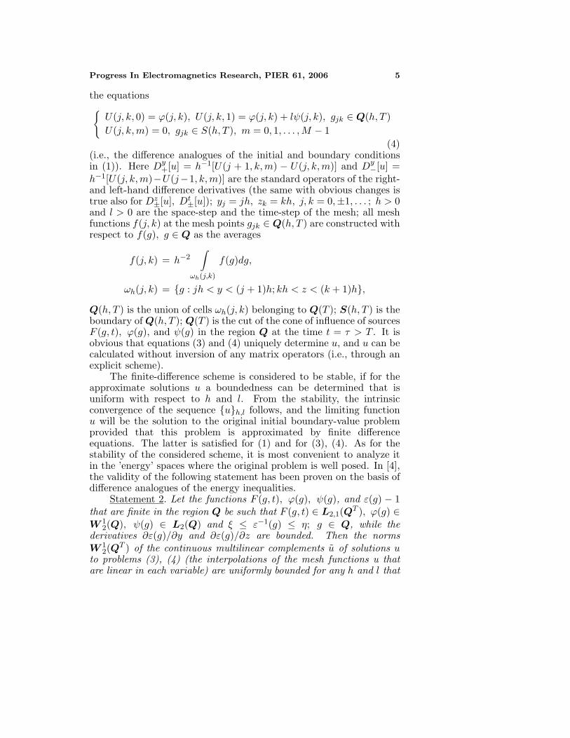
The choice of the source parameters is illustrated by the followingexample. In Fig. 2 the results of numerical experiments with

F (g, t) = 10χ[3.5 − |y|]χ[1.5 − |z + 1|] cos(β1ky + β2

)cos

(β3kz + β4

)× exp

[−(t−T )2/4α2

]cos[k(t−T )]χ(t− T )=P1(g)F1(t), (30)

are presented. This source function has seven free parameters (k, α, T ,and βj , j = 1, . . . , 4). The parameter k specifies an amplitude centerof the primary signal in the spectral domain (Fig. 2a), namely, thepoint at which an absolute value of the function

Uprim(g, k, f) =T∫

0

Uprim(g, t)eiktdt↔Uprim(g, t), t ≤ T0, t > T

(31)

is maximal. Here Uprim(g, t) represents the field generated by F (g, t)in free space. Together with α, it determines a range [k− b/α; k+ b/α]of real frequencies k, where the normilized spectral amplitudes ofUprim(g, t) (|Uprim(g, k, f)|/|Uprim(g, k, f)|) do not exceed γ. On thet-axis, the value |Uprim(g, t)|/|Uprim(g, T )| does not exceed γ out of therange T − cα ≤ t ≤ T + cα occupied by the signal Uprim(g, t). InTable 1 we give approximate values of b and c obtained [11] from thewell-known analytical representations for some fixed γ.

Parameters βj allows one to excite the oscillation of a givensymmetry class.

The source parameters obviously depend on whether rangecharacteristics or separate oscillations of an OR are of interest. Whenstudying an OR in a frequency range (Fig. 2b), k is made to agree withthe range center, while α is chosen such that the level of the normalizedspectral amplitudes of Uprim(g, t) (of the function f(g, k)) is not too low


4.0 4.5

5 15

—

0

2

1.9

3.8

2 6

—3

0

3

60 120

0 100 200

30

0

—30

U g

t

t k

k

t

( ), tprim U g( ), kprim , f~~

U g( ), k, f~~

U g( ), t

U g( ), tk~= 4.33 ~~ Re k

(a)

(b)

(c)

Figure 2. Temporal and spectral characteristics of the source (30) atg = 0, 0 (a) and of the confocal resonator (36) at g = 0.2, 0.2 (b);k = 4.2, α = 1, T = 6, β1 = 1, β2 = π/4, β3 = β4 = 0, T = 150.(c) H12,1-oscillation in the OR (34). The spatial field distribution andthe field amplitude at g = 0.5,−1; k = 4.33, α = 20, T = 60, β1 =1, β2 = π/4, β3 = β4 = 0, T = 300.

(> 0.5 is desirable). To reduce the calculating time, the left boundaryof the interval T − cα ≤ t ≤ T + cα is placed at t = 0. In order toconserve the desired spectral characteristics of the source, the value of|Uprim(g, 0)| must be negligible (0.001 ≤ γ ≤ 0.01). This requirementalong with α determine the effective duration of the signal 0 ≤ t ≤ 2T .When studying the frequency characteristics, oscillations belonging toa certain symmetry class are usually of interest. Therefore, the function


Table 1. Approximate values of b and c ensuring a given signalduration and frequency band.

γ = 0.001 γ = 0.01 γ = 0.1 γ = 0.5b ≈ 2.63 2.14 1.52 0.83c ≈ 5.25 4.29 3.04 1.66

f(g, k) must belong to the same symmetry class in its spatial structureand ensure much the same magnitudes of the coefficients C(f , k) (seeformula (23)). Then the study of spectral characteristics of an OR ina frequency range reduces to the determination of the field U(g, t) ata fixed point g ∈ QL as a function of t ∈ [0, T ] with a consequentanalysis of its transform U(g, k, f) ↔ U(g, t) (the function U(g, t) isassumed zero outside of the interval t ∈ [0, T ]).

In the study of separate oscillations u(g, k) (Fig. 2c), the interval[k − b/α; k + b/α] (k ≈ Re k) may not contain the resonance pointsadjacent to Re k, while the spectral amplitudes of Uprim(g, t) must benegligible at the ends of this interval. Clearly, this requirement can beweakened by considering the classes of symmetry of the analyzed andthe adjacent oscillations.

The source

F (g, t) = P1(g)sin[∆k(t− T )]

(t− T )cos[k(t−T )]χ(t−T ) = P1(g)F2(t) (32)

generates the signals Uprim(g, t) with a more suitable distribution ofspectral amplitudes as compared with (30) (Fig. 3). In the frequencyrange [k−∆k; k+∆k], the absolute value of the function f2(k) ↔ F2(t)remains practically constant, whereas outside of this interval we have|f2(k)| ≈ 0 for all k > 0.

The chief drawback of the sources (30) and (32) is the lack ofinformation on the singularities of the function f(g, k) in the lowerhalf-plane of the sheet Ck. The presence of poles k, their orders andlocation can be inferred only indirectly by the behavior of the functionf(g, k) in the domain of real frequencies k. To tune more precisely fora certain singular point k, one can use, for example [22], the sourcesF (g, t) with the time function like

F3(t) =1

Re ket Im k sin(tRe k) ↔ f3(k) = − 1

(k − k)(k + k∗). (33)


1.0

0.0

—1.0 50 150

0

0.6

π0.3

3 5

0 3 5

1.0

0.0

—1.0 50 150

π

0.6

π0.3

π

k

k

t

t

F ( )t2f ( )k2

~

(a)

(b)

Figure 3. The characteristics of the source given by (32): k =4.2, ∆k = 1, T = 200, T = 50 (a) and T = 100 (b).

6.3. Analysis of the Results

In Fig. 2c the source (30) separates the H12,1-oscillation from thespectrum of the following OR:

σ(g) = 2.19 · 108χ[5 − |y|]χ[4 − |z|]χ

[z2 + (y − 4.5)2 − 92

]+ χ [4 − |z +D|]χ

[(z +D)2 + (y + 4.5)2 − 92

]. (34)

Formula (34) describes the confocal copper resonator whose reflectorsare shifted relative to each other by D = 2.0. All dimensions are givenin centimeters. The subscripts m and n in the oscillation descriptorHm,n indicate the number of semi-variations of the field along y-axis and z-axis, respectively. The source is practically ‘turned-off’at t = 2T = 120, and hence, for τ = t− 2T > 0 we have from (22)

U(g, t) ≈ U(τ) = A exp(τ Im k) cos(τ Re k + a) (35)

for every fixed point g ∈ Qb. By comparing (35) with U(g, t) plottedin Fig. 2c, we obtain the following estimates: Re k ≈ k = 4.33, Im k ≈−0.0034, A ≈ 37, and a ≈ 0.79.


In the simple case considered above, it has been possible tominimize the contribution of other free oscillations into the field U(g, t)due to the absence of other eigen frequencies adjacent to k. Theanalysis becomes more complicated if two eigen frequencies k1 andk2 are close to an extent that none of them can be separated evenwith a considerable bandwidth reduction of the signal Uprim(g, t) inthe spectral domain.

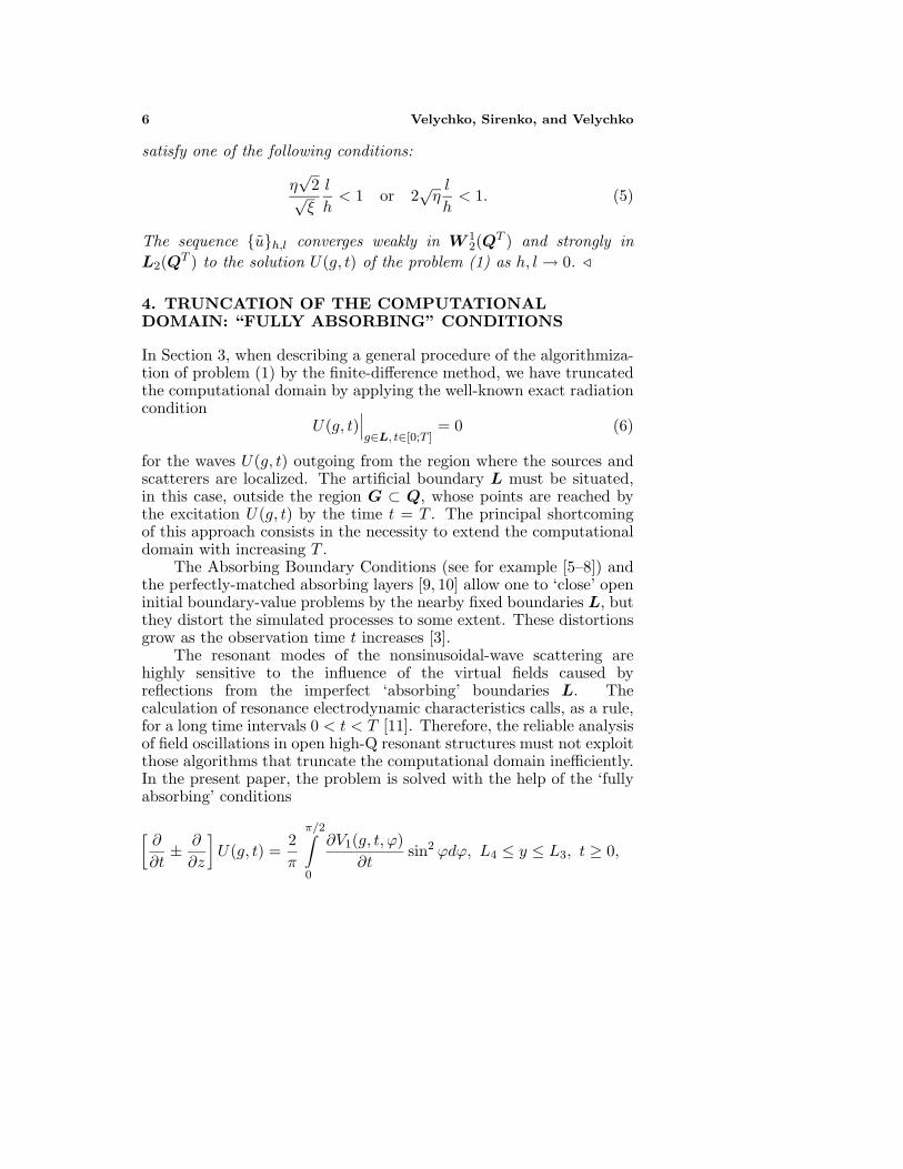
To illustrate this situation, consider (Fig. 4) the following confocalresonator

σ(g) = 2.19 · 108χ[5 − |y|]χ[4 − |z|]χ[z2 + (|y| + 4.5)2 − 92

](36)

excited by the source (30) with k = 4.235, α = 50, T = 150, β1 =1, β2 = 0.785, β3 = β4 = 0, and T = 2500. The spectral characteristicsof the source as well as its spatial configuration are such that duringthe observation period two oscillation modes H12,1 with Re k1 ≈ 4.2212and H11,3 with Re k2 ≈ 4.239 dominate concurrently in the field U(g, t)(Fig. 4a). In Fig. 4b the function U(g, t) at the point g = 0.82, 0.0is plotted for τ = t− 2T > 0.

(a)

(b)

Figure 4. To the analysis of free oscillations with close eigenfrequencies k1 and k2.


From (22) we obtain

U(g, t) ≈ U(τ) = U1(τ) + U2(τ)= A exp(τ Im k1) cos(τ Re k1)

+B exp(τ Im k2) cos(τ Re k2 + b), τ > 0. (37)

By introducing the notation Γ0(τ) = cos[τ(Re k2 − Re k1) + b] we canverify (see a model example in Fig. 4c with Re k1 = 5.1, Re k2 =5.2, A = 0.9, Im k1 = −0.002, B = −6.0, Im k2 = −0.005, b = 0.8)that:

• the curvesΓ±

1 (τ) = ±[|A| exp(τ Im k1) − |B| exp(τ Im k2)

]and

Γ±2 (τ) = ±

[|A| exp(τ Im k1) + |B| exp(τ Im k2)

]represent ‘global inner’ and ‘global outer’ envelopes of U(τ);

• for A > 0, B > 0 at the points of contact of U(τ) and Γ±2 (τ) we

have:Γ0(τ) = 1 and cos(τ Re k1) = cos(τ Re k2 + b) = ±1,while at the points of contact of U(τ) and Γ±

1 (τ) we have:Γ0(τ) = −1 and cos(τ Re k1) = − cos(τ Re k2 + b) = ±1;

• for A < 0, B < 0 at the points of contact of U(τ) and Γ±2 (τ) we

have:Γ0(τ) = 1 and cos(τ Re k1) = cos(τ Re k2 + b) = ∓1,while at the points of contact of U(τ) and Γ±

1 (τ) we have:Γ0(τ) = −1 and cos(τ Re k1) = − cos(τ Re k2 + b) = ∓1,

• for A > 0, B < 0 at the points of contact of U(τ) and Γ±1 (τ) we

have:Γ0(τ) = 1 and cos(τ Re k1) = cos(τ Re k2 + b) = ±1,while at the points of contact of U(τ) and Γ±

2 (τ) we have:Γ0(τ) = −1 and cos(τ Re k1) = − cos(τ Re k2 + b) = ±1;

• for A < 0, B > 0 at the points of contact of U(τ) and Γ±1 (τ) we

have:Γ0(τ) = 1 and cos(τ Re k1) = cos(τ Re k2 + b) = ∓1,while at the points of contact of U(τ) and Γ±

2 (τ) we have:Γ0(τ) = −1 and cos(τ Re k1) = − cos(τ Re k2 + b) = ∓1.

The above facts allow one to determine uniquely basic parametersof free oscillations possessing close eigen frequencies k1 and k2 fromthe behavior of the function U(τ) ≈ U(g, t) for τ > 0. Thus, forexample, for the case presented in Fig. 4a,b, we obtain: Re k2−Re k1 ≈0.0178, A ≈ 3.5, Im k1 ≈ −0.0005, B ≈ 18.5, Im k2 ≈ −0.00105, b ≈2.91.


7. CONCLUSION

Until recently, it was customary to analyze spectral problems of thetheory of OR in the context of FD methods. In the present work, themethodology has been developed for applying TD algorithms to theproblems of this kind. This enables the range of rigorously solvablefundamental and applied problems to be considerably extended,since the TD methods operate on practically arbitrary geometryof electrodynamic objects allowing inclusion of any kind of metal-dielectric, magnetic, or plasma inhomogeneities. At the same time,the boundary conditions truncating the computation domain are exact,and hence, they do not distort the simulated processes.

The analytical and methodological results together with theassociated software have made possible the detailed and reliablephysical analysis of transient and steady-state processes in such openstructures that are used in solid-state and vacuum electronics, resonantquasi-optics, and resonant antennas. The relevant results are to bepresented in future papers.

APPENDIX A. TABLE OF SYMBOLS

• Rn and G ⊂ Rn – the n-dimensional Euclidean space and thedomain G in it.

• Ln(G) – the space of the functions f(g), g ∈ G, such that afunction |f(g)|n is integrable in G.

• W lm(G) – the set of all elements f(g) from Lm(G) that have

generalized derivatives up to the order of l inclusive belonging toLm(G).

• W12(G) – the subspace in W 1

2(G) such that D(G) is a dense set.• D(G) – the set of finite infinitely differentiable in G functions.• L2,1(GT ) – the space composed of all elements f(g, t) ∈ L1(GT )

with a finite norm ‖f‖ =T∫

0

∫

G

|f |2dg

1/2

dt.

• W 12,0(Q

T ) – the subspace in W 12(G

T ) such that the smoothfunctions belonging to this subspace and going to zero in thevicinity of P T = P × (0, T ) form a dense set (P is the boundaryof G).

• l2 – the space of infinite sequences

a = an :

∑n

|an|2 <∞

.


• χ[f1(g)]χ[f2(g)] · · ·χ[fm(g)] – the generalized step-function suchthat it is equal to unity in the intersection G of the sets Gj =g ∈ Rn : fj(g) ≥ 0, j = 1, 2, . . . ,m and it is equal to zero inRn\G.

REFERENCES

1. Taflove, A. and S. C. Hagness, Computational Electrodynamics:the Finite-Difference Time-Domain Method, Artech House,Boston, 2000.

2. Rao, S. M. (ed.), Time Domain Electromagnetics, Academic Press,San Diego, 1999.

3. Sirenko, Y. K., S. Strom, and N. Yashina, Modeling and Analysisof Transient Processes in Open Resonant Structures, Springer,New York, 2006.

4. Ladyzhenskaya, O. A., The Boundary Value Problems ofMathematical Physics, Springer-Verlag, New York, 1985.

5. Engquist, B. B. and A. Majda, “Absorbing boundary conditionsfor the numerical simulation of waves,” Mathematics of Computa-tion, Vol. 31, No. 139, 629–651, 1977.

6. Mur, G., “Absorbing boundary conditions for the finitedifference approximation of the time-domain electromagnetic fieldequations,” IEEE Trans. on EMC, Vol. 23, No. 4, 377–382, 1981.

7. Mei, K. K. and J. Fang, “Superabsorbtion — A method to improveabsorbing boundary conditions,” IEEE Trans. on AP, Vol. 40,No. 9, 1001–1010, 1992.

8. Betz, V. and R. Mittra, “A boundary condition to absorb bothpropagating and evanescent waves in a FDTD simulation,” IEEEMicrowave and Guided Wave Letters, Vol. 3, No. 6, 182–184, 1993.

9. Berenger, J. P., “A perfectly matched layer for the absorption ofelectromagnetic waves,” Journ. Comput. Physics, Vol. 114, No. 1,185–200, 1994.

10. Sacks, Z. S, D. M. Kingsland, R. Lee, and J. F. Lee, “A perfectlymatched anisotropic absorber for use as an absorbing boundarycondition,” IEEE Trans. on AP, Vol. 43, No. 12, 1460–1463, 1995.

11. Sirenko, Y. K., L. G. Velychko, and F. Erden, “Time-domain and frequency-domain methods combined in the studyof open resonance structures of complex geometry,” Progress inElectromagnetics Research, Vol. 44, 57–79, 2004.

12. Sirenko, Y. K., “Exact ‘absorbing’ conditions in outer initialboundary-value problems of electrodynamics of nonsinusoidal


waves. Part 3. Compact inhomogeneities in free space,”Telecommunications and Radio Engineering, Vol. 59, Nos. 1–2,1–31, 2003.

13. Vladimirov, V. S., Equations of Mathematical Physics, Dekker,New York, 1971.

14. Waynberg, B. R., Asymptotic Methods in the Equations ofMathematical Physics, Publ. of Moscow State University, Moscow,1982 (in Russian).

15. Shestopalov, V. P., Y. A. Tuchkin, A. Y. Poyedinchuk, andY. K. Sirenko, New Methods for Solving Direct and InverseProblems of the Diffraction Theory. Analytical Regularization ofthe Boundary-Value Problems in Electromagnetic Theory, Osnova,Kharkov, 1997 (in Russian).

16. Colton, D. and R. Kress, Integral Equation Methods in ScatteringTheory, Wiley-Interscience Publication, New York, 1983.

17. Shestopalov, V. P. and Y. K. Sirenko, Dynamic Theory ofGratings, Naukova Dumka, Kiev, 1989 (in Russian).

18. Muravey, L. A., “Analytical extension on the Green functionparameter of the outer boundary-value problem for two-dimensional Helmholtz equation. III,” Collected Papers onMathematics, Vol. 105, No. 1, 63–108, 1978 (in Russian).

19. Hokhberg, I. Z. and Y. I. Seagul, “Operator generalization ofthe theorem about logarithmic residue and the Rouche theorem,”Collected Papers on Mathematics, Vol. 84, No. 4, 607–629, 1971(in Russian).

20. Keldysh, M. V., “On the completeness of eigen functions ofsome classes of not self-adjoint linear operators,” Advances ofMathematical Sciences, Vol. 26, No. 4, 15–41, 1971 (in Russian).

21. Melezhik, P. N., “Mode conversion in diffractionally coupled openresonators,” Telecommunications and Radio Engineering, Vol. 51,Nos. 6–7, 54–60, 1997.

22. Korn, G. A. and T. M. Korn, Mathematical Handbook forScientists and Engineers, McGraw-Hill Book Company, Inc., NewYork, 1961.

Date post:	10-Apr-2018
Category:	Documents
Upload:	trinhthien
View:	214 times
Download:	0 times

TIME-DOMAINANALYSISOFOPENRESONATORS ... In Electromagnetics Research, PIER 61, 1–26, 2006...

Documents