1 Time Value of Commercial Product Returns V. Daniel R. Guide Jr. 1 , Gilvan C. Souza 2 , Luk N. Van Wassenhove 3 , Joseph D. Blackburn 4 1 Smeal College of Business, The Pennsylvania State University, University Park PA 16802 USA 2 Robert H. Smith School of Business, University of Maryland, College Park MD 20742 USA 3 INSEAD, Boulevard de Constance, 77305 Fontainebleau, France 4 Owen School of Management, Vanderbilt University, Nashville TN 37203 USA ABSTRACT Manufacturers and their distributors must cope with an increased flow of returned products from their customers. The value of commercial product returns, which we define as products returned for any reason within 90 days of sale, now exceeds US $100 billion annually in the US. Although the reverse supply chain of returned products represents a sizeable flow of potentially recoverable assets, only a relatively small fraction of the value is currently extracted by manufacturers; a large proportion of the product value erodes away due to long processing delays. Thus, there are significant opportunities to build competitive advantage from making the appropriate reverse supply chain design choices. In this paper, we present a network flow with delays model that includes the marginal value of time to identify the drivers of reverse supply chain design. We illustrate our approach with specific examples from two companies in different industries and then examine how industry clockspeed generally affects the choice between an efficient and a responsive returns network. 1 Introduction Manufacturers and their distributors must cope with an increased flow of returned products from their customers. The value of commercial product returns, which we define as products returned for any reason within 90 days of sale, now exceeds US $100 billion annually (Stock, Speh and Shear 2002). Although the reverse supply chain of returned products represents a sizeable flow of potentially recoverable assets, only a small fraction is currently extracted by manufacturers. A large
Transcript
1
Time Value of Commercial Product Returns V. Daniel R. Guide Jr.
1, Gilvan C. Souza
2, Luk N. Van Wassenhove
3, Joseph D. Blackburn
4
1Smeal College of Business, The Pennsylvania State University, University Park PA 16802 USA
2 Robert H. Smith School of Business, University of Maryland, College Park MD 20742 USA
3INSEAD, Boulevard de Constance, 77305 Fontainebleau, France
4Owen School of Management, Vanderbilt University, Nashville TN 37203 USA
ABSTRACT
Manufacturers and their distributors must cope with an increased flow of returned products from their
customers. The value of commercial product returns, which we define as products returned for any
reason within 90 days of sale, now exceeds US $100 billion annually in the US. Although the reverse
supply chain of returned products represents a sizeable flow of potentially recoverable assets, only a
relatively small fraction of the value is currently extracted by manufacturers; a large proportion of the
product value erodes away due to long processing delays. Thus, there are significant opportunities to
build competitive advantage from making the appropriate reverse supply chain design choices. In
this paper, we present a network flow with delays model that includes the marginal value of time to
identify the drivers of reverse supply chain design. We illustrate our approach with specific
examples from two companies in different industries and then examine how industry clockspeed
generally affects the choice between an efficient and a responsive returns network.
1 Introduction
Manufacturers and their distributors must cope with an increased flow of returned products
from their customers. The value of commercial product returns, which we define as products returned
for any reason within 90 days of sale, now exceeds US $100 billion annually (Stock, Speh and Shear
2002). Although the reverse supply chain of returned products represents a sizeable flow of
potentially recoverable assets, only a small fraction is currently extracted by manufacturers. A large
2
proportion of the product value erodes away in the returns process. Most returns processes in place
today were developed for an earlier environment in which return rates were low and the value of the
asset stream was insignificant. Returns processes were typically designed for cost efficiency where
collection networks minimized logistics costs and the need for managerial oversight. For example,
Stock, Speh and Shear (2002) describe Sears’ cost-effective transportation network serving three
central returns processing centers.
Although cost-efficient logistics processes may be desirable for collection and disposal of
products when return rates are low and profit margins are comfortable, this approach can actually
limit a firm’s profitability in today’s business environment. The design of processes driven by a
narrow operational cost focus can create time delays that limit the options available for reuse. These
limited product disposition options can lead to substantial losses in product value recovery. This is
typically the case for short life cycle, time-sensitive products where these losses can exceed 30% of
product value. There is a need for design strategies for product returns that emphasize asset recovery
in addition to operating costs, and that need motivates this research.
We consider the problem of how to design and manage the reverse supply chain to maximize
net asset value recovered from the flow of returned products. Unlike forward supply chains, no
principles of design strategy for returns processing have been established. Blackburn, Guide, Souza
and Van Wassenhove (2004) hypothesize that the marginal value of time can be used to help
managers design the right reverse supply chain. Their hypotheses are supported by case studies of
several reverse supply chains. We evaluate alternative reverse supply chain designs using network
flow models capturing the effects of delays on costs and revenues. Our alternative network designs
are derived from two sources: observations of emerging practices in returns processing and the
research on design strategies for forward supply chains.
Our models are built and validated using data collected through in-depth studies of the returns
processes at Hewlett-Packard Company (HP) and Robert Bosch Tool Corporation (Bosch). These
3
two firms’ product return environments exhibit significant differences in processing and delay costs,
and we show that these should lead to alternative network designs, offering useful insights into what
drives these decisions. We subsequently use these two cases as a basis for sensitivity analysis and
test the generality of our insights.
This paper is organized as follows. In §2, we review the relevant literature. In §3, we present
an overview of the product returns system for two manufacturers, HP and Bosch, which serves as a
motivation for the model. In §4, we present the model, and theoretical results. In §5, we study ways
to improve network responsiveness. In §6, we analyze a partially decentralized network for handling
product returns. In §7, we apply the results to HP and Bosch, using empirical data from these
manufacturers. Finally, we conclude in §8.
2 Literature Review
Although manufacturers have a growing interest in extracting value from commercial product
returns, there has been little research on how to design the reverse supply chain for this purpose.
However, extensive research has been conducted on managing product return flows for the recovery
of products at their end-of-use (EOU) or end-of-life (EOL), where products are prevented from
entering the waste stream via value and materials recovery systems. Fleischmann (2001), Guide
(2000) and Guide and Van Wassenhove (2003) offer comprehensive reviews of the remanufacturing,
reverse logistics, and closed-loop supply chain research on EOU/EOL returns processes. Most of
these studies focus on cost-efficient recovery and/or meeting environmental standards. This literature
has focused on operating issues (e.g., inventory control, scheduling, materials planning) and the
logistics of product recovery. Few papers take a business perspective of how to make product returns
operations profitable (see Guide and Van Wassenhove 2001 for a discussion, and Guide, Teunter and
Van Wassenhove 2003 for a modeling example).
4
Much of the previous research on commercial product returns documents the return rates of
different product categories and the cost of processing returns. This research finds that return rates
vary widely by product category, by season and across global markets. For example, product return
percentages can vary from 5-9% for hard goods and up to 35% for high fashion apparel. Return
percentages are also typically much higher for Internet and catalogue sales. Other research has found
that, due to differences in customer attitudes and retailers’ return policies, the proportion of returned
product tends to be considerably higher in North America. Many retailers in the United States permit
returns for any reason within several months of sale. Return policies have been much more restrictive
in Europe and, consequently, return rates were markedly lower. However, return rates are rising in
Europe rapidly due to new EU policies governing Internet sales, and the entry of powerful US-based
resellers. Additionally, companies have seen an increase in commercial returns disguised as defects
from large resellers in the UK (Helbig 2002). Recent studies reported in the trade literature also
reveal that returns may cost as much as three to four times the cost of outbound shipments (Andel and
Aichlmayr 2002). Although these reports have raised management’s awareness of the problem of
product returns, the issue of how to extract more value from the returns stream has been largely
ignored.
From a marketing perspective, research examines how returns policies affect consumer
purchase probability and return rates. Wood (2001) found that more lenient policies tended to
increase product returns, but that the increase in sales was sufficient to create a positive net sales
effect. Other research has focused on the problem of setting returns policy between a manufacturer
and a reseller and the use of incentives to control the returns flow (Padmanabhan and Png 1997 1995,
Pasternack 1985, Davis, Gerstner and Hagerty 1995, Tsay 2001). Choi, Li and Yan (2004) study the
effect of an e-marketplace on returns policy in which internet auctions are used to recover value from
the stream of product returns.
Supply Chain Design Strategy
5
A number of researchers have contributed to the development of design strategy for forward
supply chains and our models are motivated by this work (Swaminathan and Tayur 2003, Fisher
1997, Lee and Whang 1999, Lee and Tang 1997, Feitzinger and Lee 1997). We are able to confirm a
set of design principles for reverse supply chains. Fisher (1997) recommends (cost) efficient supply
chains for functional products (low demand uncertainty), and responsive supply chains for innovative
products (high demand uncertainty). We observe that a (cost) efficient returns network equates to a
centralized structure and a responsive network equates to a decentralized one; we relate products with
high time value decay to Fisher’s innovative products. However, we find that in reverse supply chain
design, it is early, not delayed, product differentiation that determines profitability.
Valuing Time in Supply Chains
A significant difference between our model and previous research on reverse supply chains is
that we explicitly capture the cost of lost product value due to time delays at each stage of the returns
process. Studies of time-based competition (Blackburn 1991) have demonstrated that faster response
in business processes can be a source of competitive advantage, and other studies have shown how to
quantify the effect of time delays in traditional make-to-stock supply chains (Blackburn 2001). In
his book Clockspeed, Fine (1998) shows that the effects of speed vary across industries and product
categories, and he uses these concepts to link supply chain strategies to product architecture. This
earlier work provides the motivation for our models that specifically incorporate the cost of time
delays and its effect on asset recovery.
3 Commercial Returns at HP and Bosch
Customers may return products for a variety of reasons (see Tables 1 and 2), many of which
may be classified as non-defective. Some of these non-defective returns are new returns, because
they are essentially unused products that may be resold after visual inspection and repackaging. HP
6
estimates the cost of product returns at 2 percent of total outbound sales for North America alone
(Davey 2001). Figure 1 shows the flow for product returns in generic terms.
3.1 Case 1: Hewlett-Packard Inkjet Printers
HP’s product returns strategy is focused on recovering maximum value from the returns and
developing capabilities that would put HP in a position of competitive advantage. HP’s inkjet printer
division handled over 50,000 returns per month in North America in 1999 (Davey 2001). The most
recent trend estimates show a 20% increase. Inkjet printers have a relatively short lifecycle, with a
new model being introduced every 18 months on average.
Figure 1: Product returns process flows
Distribution Reseller
Sales
Manufacturing
ReturnsNew returns
Remanufacturing(may be multiple
facilities)
Return Stream
Returns
Evaluation
Sales (secondary market)
Products returned to the reseller are stored until transportation to the central HP returns depot
outside Nashville, TN, where credit is issued. No hard data is available on how long the returned
products spend waiting for transport at the reseller. This can vary drastically from reseller to reseller,
but HP managers believe products could spend as long as 4 weeks when the returns are stored in
areas where they are ‘out-of-sight, out-of-mind’ (Davey 2001).
Inkjet printers are delivered via truck and are unloaded and stored in holding areas at the depot
to await disposition. The time required for transportation ranges from 6 to 13 days depending on the
7
distance to be traveled. The receipt and credit issuance take an average of 4 days. After credit
issuance, returns are sorted by product line. Inkjet printers are tested, evaluated, and sent to one of
several facilities. All HP printers have an electronic counter that allows a technician to determine
how many copies have been printed.
Presently, the average remanufacturing time is 40 days. All remanufactured HP inkjet printers
are sold in secondary markets under the direction of a dedicated sales representative.
Table 1: Breakdown of reasons for commercial product returns of HP printers
Reason for
return
Description % of
returns
Procedure after return
Product defective A truly defective product – it simply
does not function as intended
20.0% Product is tested, remanufactured (low
or high touch) and sold to a secondary
market (sell as remanufactured).
Could not install The customer could not install the
product correctly. Box opened, but
product was never used.
27.5% Product is tested for number of pages
printed; if this number is zero, then the
product is re-boxed and shipped back to
the forward distribution center to be
sold as new. Otherwise it is shipped to
appropriate remanufacturing facility.
Performance not
compatible with
user needs
The product did not meet the user’s
needs. Print quality was too low,
printing speed was too slow, etc.
40.0%
Convenience
returns
The product was returned for a host of
reasons (remorse, rental, better price,
etc.)
12.5%
3.2 Case 2: Robert Bosch Tool Corporation
Bosch’s Skil line is aimed at the consumer market. These tools are reasonably priced and have
small profit margins due to the competitive nature of the market. The current product returns process
is a result of the 90-day returns policy, which is meant to attract customers.
Customers return products directly to resellers. The life cycle of power tools currently averages
6 years. Table 2 shows the primary reasons customers return products (Wolman 2003). The reseller
holds the returned tools in an RTV (return-to-vendor) cage. This inventory is held until a Bosch
salesperson is available to perform disposition on the product. The period of time between receipt of
product and disposition is again highly variable, depending on the workload of the salesperson, with
times ranging from one to four weeks (Valenta 2002). The returned products are sent to Walnut
8
Ridge, AR if a product is deemed to be a straightforward remanufacture and to Addison, IL if the
problem appears to be more technical in nature. Products are transported in bulk via trucks to the
appropriate remanufacturing facility. Products are diagnosed by technicians and remanufactured
when possible. Products are discarded if reconditioning is not possible or likely to be very expensive.
The reconditioned products are sold mainly to liquidators at an average of 15% below the retail price
for the new product.
Table 2: Returns classifications for power tools
Reason for return Percentage of returns
Consumer tools
Product defective 60%
Poor performance – does not meet
user expectations
15%
Improper marketing of tool 10%
Buyer remorse 10%
Tool used for a specific purpose then
returned (rental)
5%
4 A Simple Analytical Model for the Time-Value of Product Returns
We present an analytical model that computes the value of time in a closed–loop supply chain
and provides closed–form expressions that allow a manager to quickly compute the value of reducing
delays. In §5, we discuss specific actions aimed at reducing delays in the network. We also
developed a simulation model in ARENA that allowed us to confirm the model’s robustness under
more complex scenarios such as the presence of batching; we comment on this later.
Empirical evidence gathered at HP and Bosch suggests that the rate of commercial returns
follows a curve similar to the product life cycle, shifted to the right in the time axis, with a long
steady state period. Figure 2 shows the returns life cycle for an inkjet printer, which has a typical life
cycle of 18 months; the steady state period varies in length from seven to thirteen months. For Bosch
power tools, a typical life cycle is 6 years, with a steady state period of 5 years. In the ramp-up
period of the life cycle, most returns are used for warranties (i.e., instead of repairing defective
products in the field, the firm uses refurbished products originated from convenience returns to
9
replace these defective products), whereas in the ramp-down period their primary use is for spare
parts, after disassembly (Davey 2001).
Figure 2: Returns lifecycle for a typical inkjet printer
Start shipping
2 months 1
6 months 2
9-15 months 3
1 – Product returns increasing rapidly to stable volumes
2 – Refurbished products available
3 – End of product life, followed by a large number of stock adjustment returns
Start-up Steady State Phase-out
Returns Volume
Time
We develop a profit maximization model for the steady state period of the returns life cycle, due
to the high volumes involved, the long time frame, and the primary use of returns in the steady state
period for remanufacturing and sales at a secondary market. We model a closed-loop supply chain as
a network flow model, shown in Figure 3, where the notation is defined in Table 3. The facilities in
the closed-loop supply chain include factory, distribution center, retailer, customer, evaluating facility
for returns, remanufacturing, and the secondary market, where remanufactured products are sold. We
represent facilities by nodes, and the flow of products through the nodes is indicated in Figure 3, and
described in detail below. To avoid unnecessary confusion, our notation uses parentheses for
grouping terms, and square brackets for denoting functions, e.g., r(1 – p) denotes r times (1– p), and
c[a] denotes c as a function of a.
Similarly to Toktay, Wein and Zenios (2000), and for ease of exposition, we consider a single
retailer. In §7 we show how the model can be easily extended to multiple retailers when we apply it
10
to HP. Each node i experiences a fixed delay Wii; there are also transportation delays ij between
each pair of nodes i and j in Figure 3, except to and from the customer.
Figure 3: Closed-loop supply chain model
Distributor Retailer
Sales
Factory
Evaluation of returns Returns
pr
Remanufacturing
r
(1 ) rp
(1 ) rp r
Customer
Consumption
r
r
Sales to secondary market
(1 ) rp
f d s
r c
2m
e
11
Table 3: Notation
i, j Subscripts for nodes: f (factory), d (distributor), s (retailer sales), r (retailer returns), c
(customer), e (central evaluating facility), m (remanufacturing), 2 (sales outlet at secondary
market)
Net new sales rate at the primary market
r Total steady state return rate
p Proportion of new returns from total returns
ij Product flow rate between nodes i and j
ij Average transportation time between nodes i and j
Wij Delay between the beginning of processing at node i and end of processing at node j
Wii Delay at node i
Continuous–time price decay at primary market (i.e., % price decay per unit time)
m Continuous–time price decay at secondary market
Continuous–time discount rate
Continuous-time variable production cost decay parameter
m Continuous-time remanufacturing cost decay parameter
P[t] Unit price for new product at primary market at time t
Pm[t] Unit price for remanufactured product at secondary market at time t;
v[t] Variable production cost at time t
vm[t] Variable remanufacturing cost at time t
ijc Unit transportation cost between nodes i and j
hi
Handling cost per unit at node i; { , }i e r
[t] Profit rate at time t
Total discounted profit over steady–state period
Time t = 0 is defined as the beginning of the steady state period for returns (sales are already in
steady state at that time). Time t = T is the end of steady state for sales and returns (whichever is
earlier). Thus all nodes are in steady state for the period of analysis. The factory operates in make–to–
order mode; (1 ) rp represents the rate of orders to the factory. Products then flow from node
to node as they are processed; the flow rates between each pair of nodes ij are defined in Figure 3,
i.e., (1 )fd rp , ds sc r , cr re r , 2 (1 )em m rp , and ed rp .
Inventory is stored as finished goods at the retailer (and thus the delay Wss before the new product is
sold), and at the secondary market node (thus the delay W22 before the remanufactured product is
sold).
Consistent with empirical data obtained at HP and Bosch, we assume for both new and
remanufactured products exponential price decay functions, i.e. [ ] [0] tP t P e and
12
[ ] [0] mt
m mP t P e
, and exponential variable cost decay functions, i.e. [ ] [0] tv t v e , and
[ ] [0] mt
m mv t v e
. The continuous–time decay parameters ( and m, and m ) may or may not be
equal. All decay parameters can be viewed as a measure of industry clockspeed (see, e.g. Williams
1992, Mendelson and Pillai 1999).
There are handling costs for processing returns where ih is the handling cost per unit at facility i
(i = r for retailer and i = e for evaluating facility). Transportation and handling costs are assumed
constant over time. This is because the decay in prices and variable costs is primarily related to
material and product value erosion, which does not hold for transportation and handling costs. All
cash flows are discounted at a continuous discount factor , which represents the firm’s opportunity
cost of capital (i.e., time value of money).
For tractability, we make one assumption:
Assumption 4-1: New returns are only returned once. That is, a new return only goes through the
cycle in Figure 3 once.
Assumption 4-1 is a reasonable approximation because the fraction of returns that are returned
to the forward supply chain is very small, as we document in the case examples described later.
The sequence of events is as follows (see Figure 3):
Time t: the factory produces (1 ) rp units at a per unit cost v[t]. These units are shipped to
the distributor, where they are joined by rp new returns (produced at time loopt W , where loopW
is the delay through the loop for the network shown in Figure 3), and then transported to the
retailer.
Time fst W : the retailer sells r units at a per unit price [ ]fsP t W . After a sojourn time
with the customer, r units are returned to the retailer, where they wait until they are shipped to
the evaluating facility for sorting and credit issuance.
Time fs cet W W : after sorting, the manufacturer issues a credit of [ ]fsP t W (selling price) for
each of the r returns to the retailer. New returns rp are shipped to the forward distribution
center; non-new returns (1 ) rp are shipped to the remanufacturing facility.
13
Time fs cmt W W : non-new returns (1 ) rp are remanufactured at a per unit cost
[ ]m fs cmv t W W , and then shipped to the secondary market.
Time 2fs ct W W : (1 ) rp remanufactured products are sold at the secondary market at a per
unit price 2[ ]m fs cP t W W .
The profit rate at time t for the existing network is:
2
( , ) in net
[ ] [ ] (1 ) [ ] [ ]
[ ] [ ] (1 ) [ ] [ ]
,
ceW
r fs r r fs
r loop r m fs c m fs cm
ij ij r e r r
i j
t P t W p v t P t W e
p v t W v t p P t W W v t W W
c h h
(1)
The terms in (1) represent sales revenue for r products sold at a unit price [ ]fsP t W at the
retailer, variable production cost at the factory at time t, credit issued for r returns ceW time units
after they were sold at time fst W , difference in variable costs for new returns (i.e. new returns were
produced at loopW time units before other non-returned products and hence at a higher cost), unit
margin for remanufactured products (unit price 2[ ]m fs cP t W W minus unit production cost
[ ]m fs cmv t W W ), sum of transportation costs across all network arcs, handling costs at the
evaluating facility and retailer, respectively.
The total discounted profit over the steady state period is 0
[ ]T tt e dt , resulting in
2( ) ( )
( , )
1 1
(1 )
,
fs fs loopce
m fs c m fs cm
W W WW
r r
W W W W
r m m
ij ij r r r ei j
Pe v Pe e pv e
p P e v e v
c h h
(2)
where, for notational convenience, we define ( )[0] 1 /TP P e ,
( )[0] 1 /Tv v e , ( )[0] 1 /m T
m m mv v e
,
( )[0] 1 /m T
m m mP P e
, (1 ) /T
ij ijc c e , and (1 ) /T
i ih h e . Thus, P is the
total discounted revenue (including discounting and time–value decay) for the new product over the
life cycle T at a sales rate of one unit per unit time; the other “tilde” parameters are defined similarly.
14
The terms in (2) represent, discounted over T, the net margin for (net) new products sales
(revenues are “discounted” by the delay between production and sale), the “interest” gained by the
manufacturer as a result of returns (credit of returns to retailer is issued later than sale), the difference
in variable costs for new returns, the margin for remanufactured products, transportation and handling
costs.
For the remainder of the analysis, we introduce, for tractability, an approximation:
Assumption 4-2: Approximate 1ijW
ije W
; similar approximations are made for
, , , and m ij m ij ij ijW W W We e e e
.
Assumption 4-2 is reasonable because for real-life parameters 1ijW (similarly for
, , , and m m )–– this approximation implies a maximum error of 0.5% for the numerical examples
of §7. We do not use an approximation for , , , ,m m ijP v P v c and ih above because T is considerably
larger than any delay ijW in the network; thus ijT W .
Substituting loop ce ed dsW W W , cm ce em mmW W W , and 2 2 22c cm mW W W into (2),
and regrouping the terms:
( , )
2 22
(1 )
(1 )
(1 )
(1 ) (1 ) .
r m m ij ij r r r ei j
ed ds r fs r m m m m
ce r m m m m
em mm r m m m m m r m m
P v p P v v c h h
W p v W P p P v
W P pv p P v
W p P v W p P
(3)
An analysis of (3) allows for an easy visualization for the sources of revenues and costs in the
network, as well as the monetary effects of network delays. The first row indicates the steady state
discounted profit without accounting for delays of new and returned products in the network: total
discounted new product margins, remanufactured product margins, transportation and handling costs.
Equation (3) reveals that this base profit is decreased by the delays in the network:
(i) The delay of new returns until sale (they are delayed by the loop shown in Figure 3). Thus, a
one–day increase in ed dsW decreases expected profit by rp v , corresponding to the daily
15
decrease in total discounted variable production costs. Delays in other components of the loop
also affect new products, as explained in (ii) below.
(ii) The delay of new products to reach the consumer fsW . Thus, a one–day increase in the path
between factory and distributor decreases expected profit by (1 ) r m m m mP p P v ,
corresponding to the daily decrease in total discounted revenues for new and remanufactured
products. A one–day increase in the path from distributor to sales decreases expected profit by
a higher amount (1 ) r m m m m rP p P v p v due to its effect on new returns.
(iii) The delay of returned products to reach the evaluating facility ceW . Thus, a one-day increase in
the path from consumer to evaluating facility decreases expected profit by
(1 )r m m m mP pv p P v . The time–lag for credit issuance to retailers has a
positive effect on expected profit. The difference in variable cost for new returns and the daily
decrease in the remanufactured product value have negative effects on expected profit.
(iv) The transportation between the evaluating facility and remanufacturing, and remanufacturing
delay em mmW . Thus, a one–day increase in the path from the evaluating facility to
remanufacturing decreases expected profit by (1 ) r m m m mp P v , corresponding to the
daily decrease in total discounted net revenues for remanufactured products sold in the
secondary market.
(v) The delay incurred for transportation and sales in the secondary market 2 22m W . Thus, a
one–day increase in the path from the remanufacturing facility to the secondary market
decreases expected profit by (1 ) r m mp P , corresponding to the daily decrease in total
discounted sales revenues for remanufactured products sold in the secondary market.
We note that the value of one–day reduction in delays for the reverse network (iii)–(v) depends
on the following parameters: return rate r, decay parameters for the remanufactured product price m
and variable cost m, proportion of new returns p, remanufactured product revenue [0]mP and
variable cost [0]mv , variable production cost [0]v , and decay parameter for variable production cost
16
(the term P is numerically small in our experience). These parameters are all drivers of
responsiveness in the reverse network. To gain a better intuition, consider the special case where all
value decay parameters are equal (this is the case of HP and Bosch, studied in §7), which we denote
by . Then, the value of one day in the different links of the reverse network (iii)–(v) become
(1 )r m mP pv p P v , (1 ) r m mp P v , and (1 ) r mp P . In short, ignoring the
(numerically small) term P pv , a day in the reverse network is more valuable if the return rate is
higher, fewer new returns are diverted directly into the forward chain, the value decay parameter is
higher, the remanufactured product profit margin is higher, and the remanufactured product value is
higher. To put it differently, time compression is important in the reverse network for product returns
with high recoverable value, high value decay parameter, and high volume of remanufacturing.
In our simulation model we examined the impact of batching at the retailer, evaluation and
remanufacturing facilities and observed longer delays and, as a result, greater value decay in
products. We also examined the impact of capacity constrained facilities and the results again showed
significantly longer delays. These results support the insights gained from the analytical model, and
we therefore restrict our attention to the analytic model in the remainder of the paper.
5 Improving Network Responsiveness
The preceding analysis demonstrates the monetary benefits of decreasing delays in different
parts of the network. It allows for a time-cost analysis of responsive network designs. In this section,
we provide a simple analysis of the optimal level of responsiveness in the network. To provide
closed–form expressions, we model the delay at each node by the expected flow time through an
M/M/1 queue, except for the delay at the customer, sales at the retailer and in the secondary market,
where the delay is a constant value. Our choice of M/M/1 queues for the nodes captures the
significant congestion effects observed in practice for the relevant processing facilities and it has
been used before in supply chain modeling (e.g., Toktay, Wein and Zenios 2000; Iyer and Jain 2003).
17
It also means that there is no overtaking, that is, all products go through the supply chain on a first–
in–first–out (FIFO) mode. We note, however, that other delay expressions are possible (e.g., M/M/S
queue), although they prevent closed-form expressions. Our deterministic flow model with delays
now becomes equivalent to an M/M/1 queuing network model with the expected value substituted for
the random flow time in each node to compute the total expected profit over T.
Denoting by i the mean processing rate at node i, and using the expressions for expected flow
time for an M/M/1 queue, the expected delays Wij are computed as follows:
1 11/
(1 )fs fd ds s
f r d r
Wp
, (4)
1 1 1
ce re
c r r e r
W
, (5)
1
(1 )cm ce em
m r
W Wp
, (6)
2 2 21/c cm mW W , and (7)
1
1/ds ds s
d r
W
. (8)
After substituting (6)–(8) into (3), we obtain:
( , )
(1 )
1 1/ (1 )
(1 )
1 (1 )
(1 )
r m m ij ij r r r ei j
ed ds s r fs r m m m m
d r
ce r m m m m
em r m m m m
m r
P v p P v v c h h
p v W P p P v
W P pv p P v
p P vp
2
2
1(1 )m r m mp P
(9)
To improve network responsiveness we can increase i at each node (retailer, evaluating and
remanufacturing facilities), and decrease the average transportation times ij (by co–location of
facilities, or faster transportation modes). Before analyzing these alternatives, we note that is a
18
separable function in each delay variable i (that is, 2 / 0i j for i j ), and thus a sufficient
condition for (9) to be jointly concave in i, for all i, is that 2 2/ 0i for all i.
5.1 Increasing Processing Rate of Returns at the Retailers or Evaluating Facilities
Improving responsiveness r at the retailer requires investments by the manufacturer according
to the unit handling cost [ ]r rh , where we make explicit the dependence of the handling cost with the
processing rate. At Bosch the returns are held at the retailer until a Bosch representative makes a
disposition and shipment decision. Bosch can increase the processing rate at each retailer by
increasing the number of visits, which may require more service personnel. Similarly the
manufacturer can also improve the processing rate of returns at the central evaluating facility e .
This would again involve investments in workforce for parallel processing, or investments in sorting,
picking, and routing technology.
To find the optimal level of responsiveness *
i , we apply the first order condition to (9),
recalling that , ,i i r e impacts ceW according to (5):
*
2*
(1 )0 [ ], ,
m m m m
i i
i i r
P pv p P vh i r e
. (10)
Sufficient conditions for (3) to be jointly concave (such that the solution to (10) is sufficient for
optimality) are that (i) [ ]i ih be a convex function (including a linear function which is a reasonable
assumption as stated below), and (ii) that (1 ) m m m mp P v P pv , that is, remanufacturing
margins are higher than the net (negative) impact of the time lag for returns (i.e., difference between
time–value of money for credit issuance and production cost lag for new returns), since
2 2
3
(1 )/ 2 [ ]
( )
m m m m
i r r i i
i r
P pv p P vh
,
which is strictly negative if these two conditions are satisfied.
19
Now, assume a linear function for the unit handling cost as a function of the processing rate for
returns, i.e., [ ]i i i i ih a b . This linear function can be justified because return handling
operations are labor intensive (Davey 2001). Then, [ ]i i i i ih a b , where (1 ) /T
i ia a e and a
similar expression holds for ib . For this linear cost case, (10) yields:
*(1 )
, ,m m m m
i r
i
p P v P pvi r e
a
. (11)
We note that (11) has the solution form of a classic queuing design problem: find the optimal
processing rate at an M/M/1 queue that minimizes the expected cost rate (see, e.g., Gross and Harris
1998, p. 304), with waiting cost rate (1 ) m m m mp P v P pv and service cost rate r ia .
Only a fraction 1 – p of all returns r are remanufactured and sold at a revenue of mP with an
“interest rate” m . This revenue is decreased by the total discounted variable remanufacturing costs
mv , which decrease at a rate m . In addition, the waiting cost rate should be decreased by the time–
value of money amount corresponding to the daily profit increase of a delayed credit issuance to
retailers P , but increased by the daily decrease in total variable cost of production for new returns.
The optimal return processing rate at either retailer or evaluating facility is not influenced by
transportation costs, but it is directly influenced by the remanufactured product margin. Low margins
result in designs with a low level of responsiveness. A higher remanufacturing price decay parameter
m and a higher variable cost decay parameter (higher clockspeed) increase the waiting cost rate
(numerator in the square root of (11)). This increases processing capacity (lowers the waiting time)
leading to a more responsive returns network design.
A similar analysis can be conducted for the optimal level of responsiveness in the forward
distribution network, i.e., i , , ,i f s d . However, this requires modeling specific costs associated
with a level of responsiveness at the factory (increased transportation frequency to the distributor),
distributor (more frequent deliveries to retailers), and retailer (advertising, promotion, and pricing),
and the focus of this paper is not on forward supply chains.
20
5.2 Increasing Transportation Responsiveness
Transportation responsiveness in the network can be influenced by design choices such as co-
location of facilities or selecting faster transportation. For example, if the firm co–locates the
remanufacturing and the evaluating facilities, then em = 0, and profits increase by
(1 )em r m m m mp P v , according to (3).
Regarding transportation modes, each of the unit cost parameters ijc (or ijc ) is a function of
transportation time ij , that is, [ ]ij ijc . Consider the design option of moving from ground to air
transportation. The savings may be computed as the product of the value of a one–day delay
reduction on that corresponding arc of the network (§4) and the number of days saved. The
computed savings may be compared with additional transportation costs of going from ground to air.
6 Preponement: Decentralized Returns Network
In this section we analyze the drivers of alternative structural designs. Figure 3 represents the
typical centralized industrial returns evaluation and credit issuance network design where all
commercial returns are shipped to a central facility for economies of scale. The benefits in
economies of scale for evaluation and credit issuance are clear. Alternatively, consider an innovative
design where new returns are sorted and immediately re–stocked at the retailer. This decentralized
design reduces transportation costs, utilization at the central evaluation facility, and consequently the
delay of other returned products. This, in turn, increases their value in the secondary market. We call
this decentralized design concept preponement (or early product differentiation) to distinguish it from
postponement (or late product differentiation), typical in forward supply chains. Both HP and Bosch
are considering the use of preponement.
With preponement, additional work is required at the retailer to handle and re–package the
returns. Without any capacity adjustment from the existing configuration, the processing rate at the
retailer with preponement is evidently lower than in the existing configuration; thus a capacity
21
increase may be warranted. The retailer may need to hire and train workers to perform this task and
maintain extra packaging material at the stores. To gain retailer cooperation, the manufacturer may
need to offer incentives. Alternatively, the manufacturer could periodically send workers to the
retailer’s site to handle the returns, similar to Vendor Managed Inventory (VMI).
With preponement, there is no need to separate new returns from other returns at the evaluating
facility, although the facility still has to issue credit to returns and route them to the appropriate
remanufacturing facility. Further, that node experiences a lower flow of products ( (1 )p
re rp as
opposed to re r ). Without any capacity adjustment from the existing configuration, the
processing rate at the evaluating facility with preponement is evidently higher; thus, a capacity
decrease may be attractive.
The decentralized design network is shown in Figure 4. We use a superscript p to denote, when
different, parameters for this proposed preponement network. The flow rates between each pair of
nodes are p
rs rp , (1 )p
re rp , (1 )p
ds rp , and 0p
ed ; other flows are as before. As in
§4, we do not assume any functional form for the delays at the nodes to keep our results general.
Figure 4: Closed-loop supply chain with preponement: new returns handled at retailer
Distributor Retailer
Sales
Factory
Evaluation of returns Returns
pr
Remanufacturing
r
(1 ) rp
(1 ) rp r
Customer
Consumption
Sales to secondary market
(1 ) rp
(1 ) rp
f d s
r c
2m
e
(1 ) rp
An analysis similar to that performed in §4 provides the total discounted profit over the steady
state period of the lifecycle:
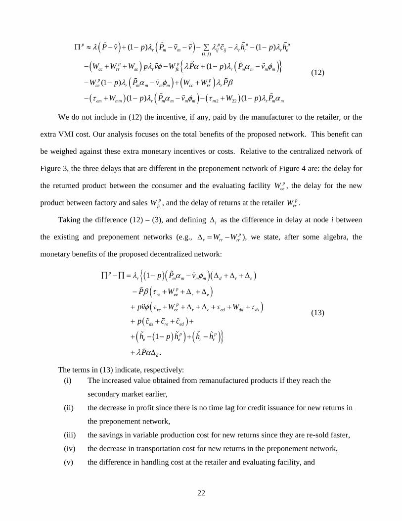
22
( , )
2 22
(1 ) (1 )
(1 )
(1 )
(1 ) (1 )
p p p p
r m m ij ij r r r ei j
p p
cc rr ss r fs r m m m m
p p
ce r m m m m cc rr r
em mm r m m m m m r
P v p P v v c h p h
W W W p v W P p P v
W p P v W W P
W p P v W p P
m m
(12)
We do not include in (12) the incentive, if any, paid by the manufacturer to the retailer, or the
extra VMI cost. Our analysis focuses on the total benefits of the proposed network. This benefit can
be weighed against these extra monetary incentives or costs. Relative to the centralized network of
Figure 3, the three delays that are different in the preponement network of Figure 4 are: the delay for
the returned product between the consumer and the evaluating facility p
ceW , the delay for the new
product between factory and sales p
fsW , and the delay of returns at the retailer p
rrW .
Taking the difference (12) – (3), and defining i as the difference in delay at node i between
the existing and preponement networks (e.g., p
r rr rrW W ), we state, after some algebra, the
monetary benefits of the proposed decentralized network:
1
1
.
p
r m m m m d r e
p
re ee r e
p
re ee r e ed dd ds
ds re ed
p p
e e r r
d
p P v
P W
pv W W
p c c c
h p h h h
P
(13)
The terms in (13) indicate, respectively:
(i) The increased value obtained from remanufactured products if they reach the
secondary market earlier,
(ii) the decrease in profit since there is no time lag for credit issuance for new returns in
the preponement network,
(iii) the savings in variable production cost for new returns since they are re-sold faster,
(iv) the decrease in transportation cost for new returns in the preponement network,
(v) the difference in handling cost at the retailer and evaluating facility, and
23
(vi) The increased value of new product sales due to reduced delay at the distributor, as a
consequence of new returns no longer being routed there.
With the exception of the last term dP , which is likely to be small in practice since new
returns constitute a small percentage of the flow of products through the distributor in the existing
network ( d is a small number), the return rate r multiplies the entire right–hand side of (13), that
is, r is a scaling parameter for the benefits of preponement. Drivers of the attractiveness of
preponement design include, as before, decay parameters for the remanufactured product price m
and variable cost m, the decay rate for variable production cost , proportion of new returns p, the
revenue and costs parameters [0]mP , [0]mv , [0]v , transportation and handling costs (again, the term
P is numerically small in our experience). We develop two general propositions providing insights
into three major drivers of attractiveness of the preponement design, i.e., the continuous-time variable
production cost decay parameter , the variable cost v[0], and the proportion of new returns, p .
Proposition 1: The benefits of preponement p are increasing in and v[0] if the time
difference for restocking a new return between the existing network (via the evaluating facility) and
the preponement network (at the retailer only) is positive, that is:
0re ee ed dd ds rK W W . (14)
Proof: The third term of (13) can be written as r pv K or ( )1
[0]Te
r pv K
, where K is the term
in parenthesis that multiplies pv in (13). This term, the only in p that includes and v[0], is
increasing in and v[0] if K > 0, which results in (14), after we write p
e ee eeW W .
It is possible that the benefits of preponement p be positive (or negative) for all
meaningful values of ; otherwise Proposition 1 implies that there is a such that a decentralized
(preponement) network design is preferred if ; else a centralized network is appropriate.
Condition (14) holds for most returns networks because it only requires that all the delays for new
returns in the original network exceed the delay at only the return node in the preponement network.
A similar result can be derived for the other design driver p:
24
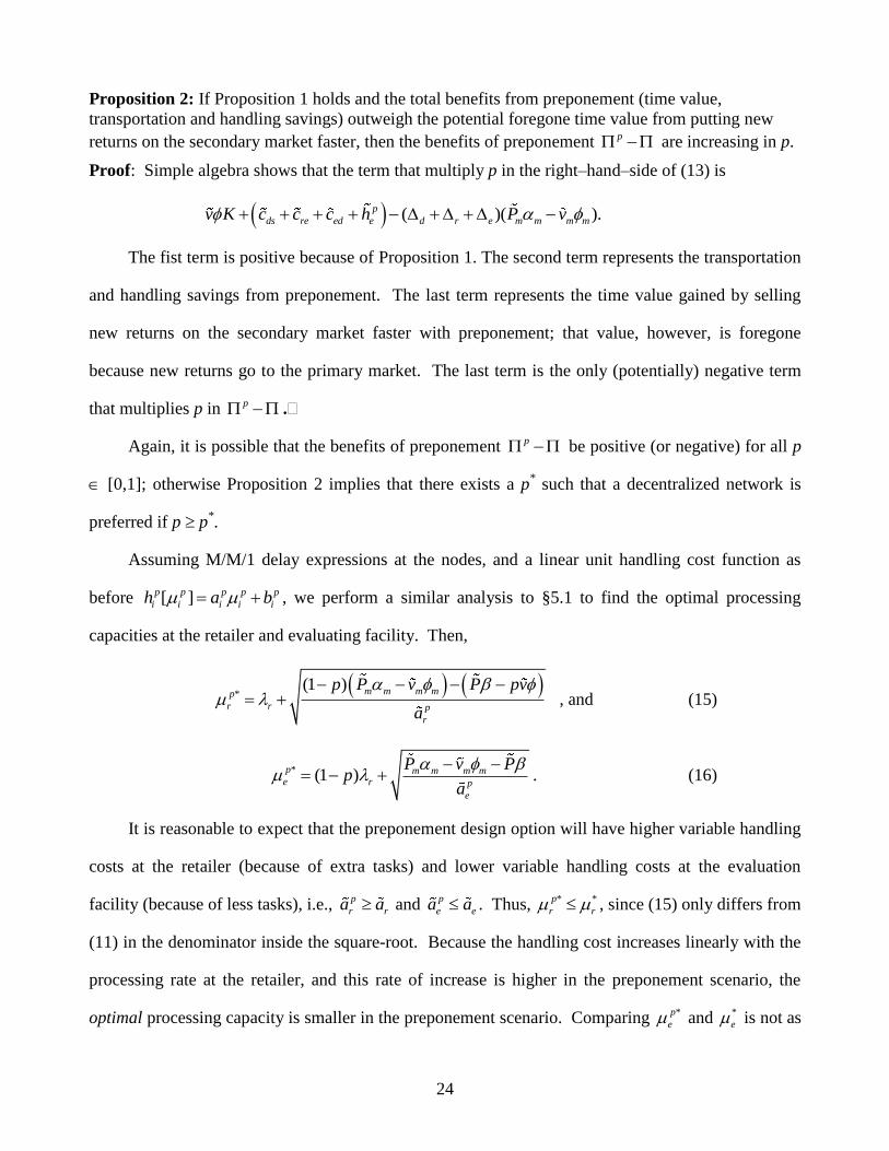
Proposition 2: If Proposition 1 holds and the total benefits from preponement (time value,
transportation and handling savings) outweigh the potential foregone time value from putting new
returns on the secondary market faster, then the benefits of preponement p are increasing in p.
Proof: Simple algebra shows that the term that multiply p in the right–hand–side of (13) is
( )( ).p
ds re ed e d r e m m m mv K c c c h P v
The fist term is positive because of Proposition 1. The second term represents the transportation
and handling savings from preponement. The last term represents the time value gained by selling
new returns on the secondary market faster with preponement; that value, however, is foregone
because new returns go to the primary market. The last term is the only (potentially) negative term
that multiplies p in p .
Again, it is possible that the benefits of preponement p be positive (or negative) for all p
[0,1]; otherwise Proposition 2 implies that there exists a p* such that a decentralized network is
preferred if p p*.
Assuming M/M/1 delay expressions at the nodes, and a linear unit handling cost function as
before [ ]p p p p p
i i i i ih a b , we perform a similar analysis to §5.1 to find the optimal processing
capacities at the retailer and evaluating facility. Then,
*(1 )
m m m mp
r r p
r
p P v P pv
a
, and (15)
* (1 )p m m m me r p
e
P v Pp
a
. (16)
It is reasonable to expect that the preponement design option will have higher variable handling
costs at the retailer (because of extra tasks) and lower variable handling costs at the evaluation
facility (because of less tasks), i.e., p
r ra a and p
e ea a . Thus, * *p
r r , since (15) only differs from
(11) in the denominator inside the square-root. Because the handling cost increases linearly with the
processing rate at the retailer, and this rate of increase is higher in the preponement scenario, the
optimal processing capacity is smaller in the preponement scenario. Comparing *p
e and *
e is not as
25
straightforward since the lower value of p
ea tends to increase *p
e relative to *
e . However, the lower
flow of returns (1 ) rp through the evaluation facility tends to decrease *p
e relative to *
e . For
larger values of p, it is clear that the lower flow effect will tend to dominate (16). In the limit, when p
= 1, *p
e = 0, and * *p
e e clearly holds.
In the next section, we apply our theoretical results to HP and Bosch, and perform a
sensitivity analysis on the key drivers of responsiveness and preponement design alternatives.
7 Application of Model Results
In this section, we apply the theoretical results to actual data from HP and Bosch. The main
differences in parameter values for the two firms are product value, life cycle length, value decay
parameters, demand, and return rates. Many of the parameter values are approximately equal for
both firms, and for reasons of confidentiality, we use common representative numbers assumed fixed
throughout the numerical analysis: a 25% gross margin for new products ( [0]/ [0]v P = 0.75), a 15%
price discount for the remanufactured product relative to the new product ( [0]/ [0] 0.85mP P ), and a
5% yearly discount rate ( = 1.4x10⁻⁴
).
The price decay parameters for remanufactured and new products are approximately the same
( m ) within each company, albeit different between companies. Although different components
decay at different rates, we estimate that the overall manufacturing cost of a product decays at a rate
roughly equal to the final product’s price decay, that is, m m . For this reason, we use a
single value decay parameter for each company. This assumption brings parsimony to the analysis
without compromising insights or the order of magnitude of the results. The units of analysis
throughout are a full truckload of returned products and a time of one day.
7.1 Hewlett-Packard Inkjet Printers
A delivery truck contains an average of 250 inkjet printers. The median price of an HP inkjet
printer is $200, and thus P[0] = 250$200 = $50,000. For inkjets, T = 395 days (13 months), returns
26
are 5% of net sales, so / 0.05r . The daily return rate averages r = 6.67 trucks, p = 1/3, and the
common value decay parameter is = 1.43x10⁻³
(1% per week). The remanufacturing cost is
approximately 7.5% of the retail price of a new product, that is, [0]/ [0]mv P = 0.075.
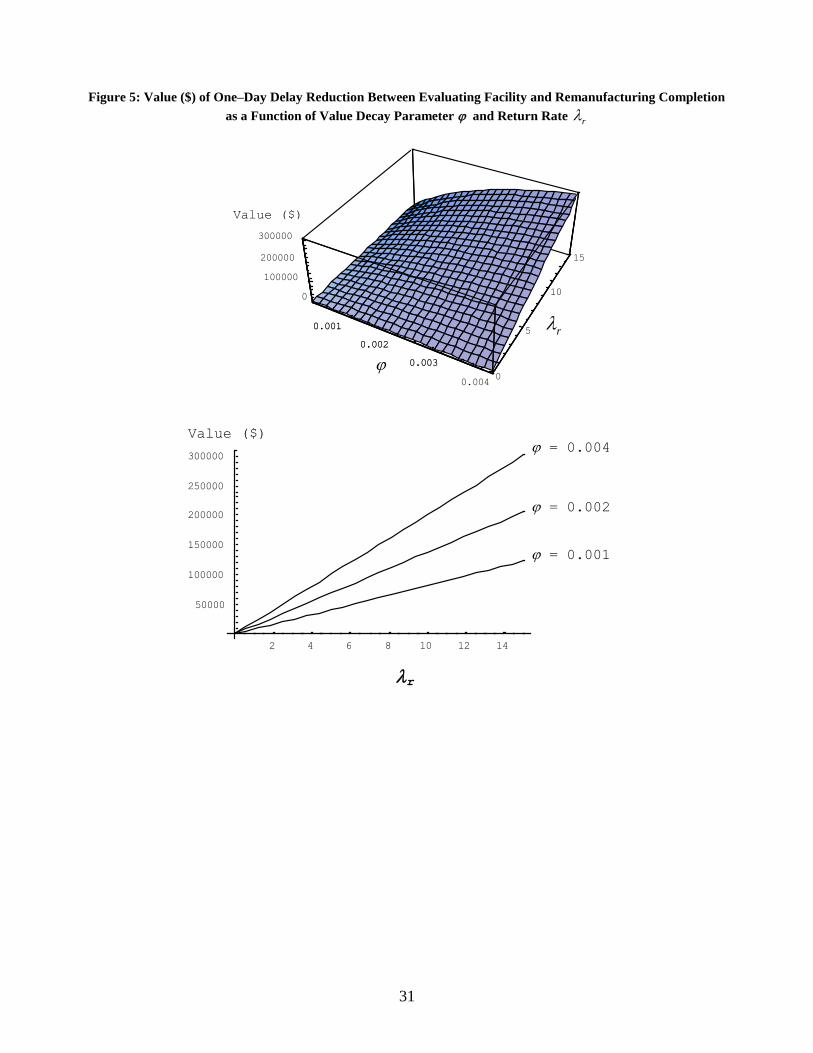
Our analysis shows the values of a one–day reduction between different facilities in the returns
network: $35,069 between the evaluating facility and distributor, $93,797 between the customer and
evaluating facility, $72,475 between the evaluating facility and remanufacturing, and $79,489
between remanufacturing and the secondary market, respectively. Managers indicate that lead–time
reduction in the forward network is currently being pursued at the level of hours, not days. However,
opportunities for significantly reducing lead–times abound in HP’s reverse supply chain. The sojourn
time at retailers, delay between retailers and process completion at the evaluating facility, and delay
between the evaluating facility and remanufacturing completion average 10, 8 and 40 days
respectively. We analyze each opportunity separately below.
First, consider the retailer returns processing capacity. For a more realistic analysis, consider
multiple retailers. For example, using 1,000 identical retailers with an average sojourn time of 10
days, and assuming M/M/1 delays at the retailer implies 1/( /1000)r r = 10, or a current return
processing capacity of r = 0.1067. If we decrease the average sojourn time by two days (and save
approximately $180,000) with the same rate of returns, this implies r = 0.1317, or a 23% increase
in returns processing capacity. To find the optimal processing capacity (11), we require an accurate
estimate of handling costs at the retailers.1
Second, consider transportation to, and sojourn time at, the evaluating facility. Managers at HP
believe that this delay can be cut from its current 8 days to 2 days, resulting in lifecycle savings of
approximately half a million dollars. Finally, the largest opportunity lies in the long delays for
shipment from the evaluating facility until completion of the remanufacturing operation, which is
1 We note that the conditions (i) and (ii) for optimality of (11), which are described in the paragraph after (10), are both
satisfied. Condition (i) is naturally satisfied because (11) assumes linear handling costs. Condition (ii) is satisfied
because (1 ) m m m mp P v = 10,866 > P pv = –3,189.
27
currently 40 days. Management believes that a reasonable goal for this delay is 20 days. Achieving
this goal implies a lifecycle savings of $1.45 million. We note that our estimates are conservative,
since we do not explicitly account for savings in working capital and the corresponding reduction in
inventory holding costs. Thus, it appears worthwhile for HP to consider a responsive network design.
We estimate the current discounted lifecycle value of preponement for HP (13) to be roughly
$4.0 million, using the following assumptions: (i) retailers are situated at an average of 1000 miles
from the evaluating facility; (ii) the truckload transportation rate is $1.3/mile2; (iii) the likely increase
in handling cost at the retailer is offset by the likely decrease in handling cost at the evaluating
facility, and, consequently, the difference in total handling costs (across retailer and evaluating
facility) between the current and preponement scenarios is negligible, and (iv) the difference in
delays between the current and preponement scenarios is negligible (i.e., 0r e ; 0d ). Of
these $4.0 million, roughly 20% are related to the time value savings in variable costs for new returns
(third term in (13)), 82.7% are related to savings in transportation costs (fourth term in (13)); the
second negative term in (13) is small at –2.7%; the first and last two terms in (13) are zero by our
assumptions. It should be clear from these rough-cut calculations that HP has a keen interest in a
more detailed analysis of the practical implications of the preponement option. In a more detailed
analysis, HP would also need to estimate the possible increase in total handling costs with
preponement, which we assumed to be negligible in the above calculation. We note that HP has
developed a hand-held IT device that shows the condition of the returned product. Other firms, such
as Pitney-Bowes and ReCellular, Inc., use visual grading standards to provide guidance in grading
product returns. Both of these actions reduce the reliance on skilled labor and may make
preponement a more attractive alternative.
2 This estimate of transportation rate is based on a US DOT report http://ops.fhwa.dot.gov/freight/documents/bts.pdf