Page 1
1
Title:
Forecasting Chinese corporate bond defaults: A comparative study of market vs
accounting- based models
Michael Peng1*, DongKai Jiang
2, YingJie Wang
3
1 Boston Consulting Group, 10 Hudson Yards, New York City, NY 10001, USA;
2 Witzcredit
Risk Analysis, 362 Milford Court, New Town, PA 18940, USA; 3 KPMG, 5001 Shennan E Rd,
DiWang, LuoHu District, Shenzhen , GuangDong Province, China 518001
* Correspondence to: Michael Peng, Email: [email protected] ; Tel: Tel 215-300-9631
Abstract
This paper provides the first empirical study on bond defaults in China market, overcoming the
deficiencies of the existing methods, which suffer from lack of actual default data for back
testing. With newly available bond default data, we analyzed the roles of market variables vs
accounting variables under various models. While we found Merton’s market-based structural
model and KMV’s Distance to Default exhibits languid discriminating power compared to
hazard models with carefully constructed predictors, other market variables carry significant
information about bond default and could help improve on models with accounting variables
only. This implies that the collective intelligence of the market could somehow mitigate the
distortion caused by misreported accounting information. We found model performance can be
improved significantly by adding predicting variables linking individual financial measure to the
broader market performance, such as relative margin, business environment proxy introduced in
this paper. This study not only sheds light on the default behavior of Chinese bond market but
also provides a promising approach to improve the variable selection process.
Key words: Bond default; Chinese bond default; bankruptcy forecast; hazard model; Merton
model; accounting variables; Z-score; LASSO regression
JEL: B41, C58, F65, G15, G17, G32, G33
Page 2
2
1. Introduction
China, the world’s third largest bond market, has been experiencing a notable spike of defaults
due to economic slowdown since late 2017. Corporate bond default cases surged to 47 in 2018
from just 10 in 2017, with a total principal amount of 110.5 billion yuan ($16.3 billion), amid a
trade war with the United States (See Fig 2 below), adding to worries about risks to the economy.
Companies rushed to sell new bonds in China in 2018, as Beijing loosens financial conditions to
shore up businesses in a weakening economy, by lowering reserve requirements for banks five
times in little over a year, encouraging them to lend more to aid an economy that has been hit by
trade tensions with the U.S. and an earlier campaign against financial risk. While China has
eased monetary policy, Chinese banks are still reluctant to lend. That has pushed companies into
the bond markets; As Fig. 1a shows, the total issuance hit record in 2018. However, the
issuance boom mostly
were mostly driven by
state-run firms, while
financially weaker
private companies
struggle to get funding.
Only 78 out of the 657
bond issuers are private.
Note that there are
apparently some signs of
mispriced risk. Gloomy
economic outlook, wave
of issuance and defaults
would normally lead investors to demand a premium before buying bonds. Instead, they have
lapped them up, making it cheaper for China’s companies to borrow. As shown in Fig.1b, yield
on five-year corporate bonds with a AAA domestic rating, a grade mostly held by state-run
enterprises, have fallen to 3.81% from 5.40% in the past year. But the yields on AA- 1debt have
declined just 0.05 percentage point to 6.87%.
1 This rating is China’s equivalent of junk, and debt with this status is mostly issued by private firms.
Page 3
3
In general, there are three modeling approaches for default forecasting: i) Accounting
variables based statistical model (including Altman Z score models); ii) market based models,
which include “Structural model 2
“(Merton 1974) extracting credit
information from equity market and
Reduced Form 3 model which
deduce default information from the
price of traded-bond); iii) hybrid
model (containing both above types
of variables). For an excellent
review of these models, see
Campbell (2008) and Bauer (2014).
Bauera, et al 2014, using UK annual
data from 1979 to 2009, compared
these approaches and concluded that the hazard model outperformed the other two alternatives
while accounting-based Z-score has more predictive power than contingent-based approach.
Agarwal (2008) reached similar conclusion using a different source of UK data.
Forecasting defaults in Chinese bond market, however, has been a challenge since no
empirical study has been done using actual default data. This is understandable because there had
been no official default event until mid-20144. The absence of the default event data not only
makes it hard to build a true statistical model taking all relevant risk drivers into account, but
also render it impossible to validate any alternative models such as Merton’s structural model or
reduced form model. Almost without exception, the literature on the credit risk of public listed
firms in China used some default proxies. The most widely used proxy is the Special Treatment
2 A full description of Merton’s underlying assumptions and its wide application can be found in an excellent review
by Sundaresan (2013).
3 For a good theoretical review of reduced form, see for example, Jarrow and Protter (2004). However, the bond
price, which usually heavily depends on credit rating in the West, is much less a reliable indicator for risk in China.
As well as questions on the lack of secondary market liquidity, another issue is the objectivity of China’s domestic
rating agencies, which are often state owned. In fact, more than 90% of Chinese corporate bonds are rated AA or
above, and risk differentiation is not easily done form rating per se. Moreover, the high ratings are not recognized in
overseas markets.
4 It was Shanghai Chaori Solar private company
Page 4
4
(hereafter ST)5, a delist warning sign designated by the regulators. (see Chen, 2014; Yang ,2010;
Zhang et.al, 2010; Zeng and Wang, 2013; Ren 2011). It can be shown that, however, ST is not a
reliable default. For example, Cerrato et al (2106) found that the spread of default probability
between ST firms and non-ST firms is larger before 2006, but it narrows afterwards. This is not
consistent with empirical default fact. In addition, high default probabilities could cause a
delisting but not vice versa; i.e. the default event is not the unique reason for delisting a firm.
Looking at the empirical results (both ‘default’ and ‘post-default’), ST is not significant,
confirming that ST may not be directly related to actual default.
In theory, the market-based model is superior since it should timely reflect investor’s
collective intelligence about the firm’s financial and operating status. However, this is not
necessarily the case in reality given the degree of market efficiency. Of course, the effectiveness
of the accounting-based model to assess the firm’s credit risk hinges upon the quality of the
information contained in the financial statements. It is for this reason that the superiority of one
model over the other is closely related to that country’s accounting system and the efficiency of
its financial markets, and should be an empirical question. By comparing the outcome built on
data from Taiwan (a relatively more mature and developed security market), with mainland
China (a less developed market), Liu et al (2010) concluded that the underperformance of the
market based model can somehow be attributed to the invalidity of efficient market assumption
implicit in Merton’s model. Further, the secondary market trading is usually very lethargic to say
the least. This low liquidity makes it hard for investor to derive default information from trading
information, rendering “reduced form” model ineffective. To our knowledge, one of most cited
paper combining Merton’s approach with statistical model was by Daniel Law and Shaun (2015)
from IMF (“IMF paper” hereafter), which linked a set of balance sheet variables to the PD
implied from the Chinese equity market using an enhanced Merton model (with jump
component).
Armed with the latest bond default data, this paper is to explore the most appropriate--
methodologically sound and empirically robust approach in forecasting default of Chinese
corporate bond by assessing which variables are more predictive. Classic hazard models are
compared to those deriving Probability of Default (PD) from equity market (i.e. Merton’s
approach). First, we will re-estimate several well-known default forecasting models (Shumway
5 When a stock is marked as *ST, its trading is suspended for one accounting year.
Page 5
5
2001, Campbell 2008, Jarrow 2004, Zmijewski 1984). Then we will test a few discrete hazard
models with a set of variables characterizing Chinese issuers and the market, including Altman’s
ZChina
score (re-estimated with the new data) and Merton’s Distance to Default computed from
the China market. In particular, we are to assess the discriminating power of “IMF” paper
mentioned above so that we can directly compare a model using Merton implied PD with that
using actual default as the dependent variable. For all the limitation of the data6, we were able
to obtain comparable results (in terms of coefficient sign, significance and predictive power)
with classic models applied to mature market such as US. We found the IMF model, with the
dependent variable being the Merton implied PD, under-performs the alternative specifications
using actual default event information. On the other hand, we found while the Distance to
Default under Merton’s framework exhibits languid discriminating power, other market variables
such as equity return and relative market cap (see RSIZE in Table A in Appendix) do carry
valuable information about bond default and help improve on models with accounting variables
only. Finally, we found several of our proposed models stand out as the best performing ones
with quite a few predictors we constructed quite robust in boosting predictive power. These
variables include: rela_margin, a variable linking individual firm profitability to the sector
median, nega_margin, a proxy for business condition and Altman’s Chinese Z -score re-
estimated with actual default data.
The paper proceeds as follows: the next section describes data sources and in Section 3
where we discussed the specifications of the empirical models to be tested. Results were reported
in Section 4, which covered performance comparison among models and out of-sample tests. In
Section 5, we presented case studies in which we illustrated how well the models forecasted
default risk for individual Chinese firms. Conclusions were drawn in Section 6, along with
Caveats.
2. Sample Selection and Data Description
2.1 Historical default events in China: a brief description
Corresponding with the growth and increasing openness of the bond market is an upsurge
in risk. Bond defaults in China have historically been quite rare. Defaults on domestically issued
bonds were non-existent and the majority of bonds were issued by large state-owned enterprises
6 The default sample size is still relatively small. In particular, among the defaulted companies, only 20 of them are
listed firms as of January, 2019.
Page 6
6
with an implicit guarantee of government support. As a result, yield spreads in the corporate
bond market provided investors little information on the actual riskiness of corporate issuers.
Things began to change after Chaori, a private solar panel manufacturer, became the first
company to default on a domestic bond in March 2014. Over the following two years, several
more firms have defaulted, postponed payments or restructured debt, including several large
state-owned enterprises. There were 19 bond issuers defaulted in 2015 and a whopping 47
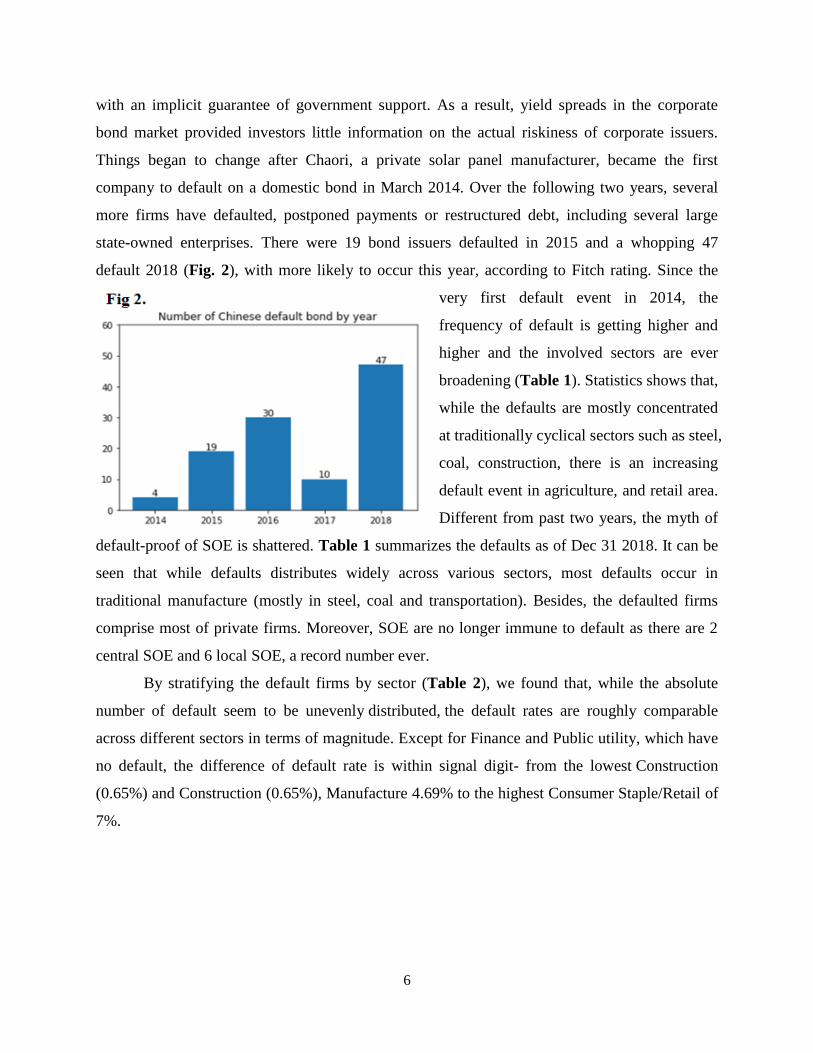
default 2018 (Fig. 2), with more likely to occur this year, according to Fitch rating. Since the
very first default event in 2014, the
frequency of default is getting higher and
higher and the involved sectors are ever
broadening (Table 1). Statistics shows that,
while the defaults are mostly concentrated
at traditionally cyclical sectors such as steel,
coal, construction, there is an increasing
default event in agriculture, and retail area.
Different from past two years, the myth of
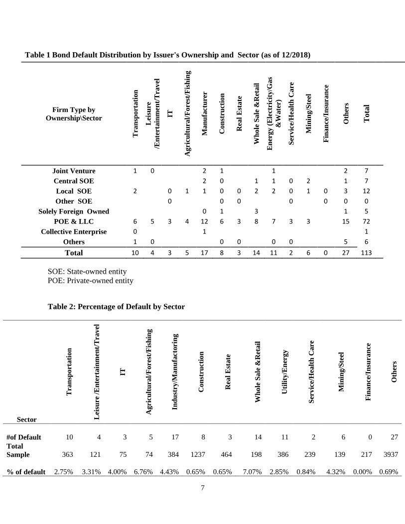
default-proof of SOE is shattered. Table 1 summarizes the defaults as of Dec 31 2018. It can be
seen that while defaults distributes widely across various sectors, most defaults occur in
traditional manufacture (mostly in steel, coal and transportation). Besides, the defaulted firms
comprise most of private firms. Moreover, SOE are no longer immune to default as there are 2
central SOE and 6 local SOE, a record number ever.
By stratifying the default firms by sector (Table 2), we found that, while the absolute
number of default seem to be unevenly distributed, the default rates are roughly comparable
across different sectors in terms of magnitude. Except for Finance and Public utility, which have
no default, the difference of default rate is within signal digit- from the lowest Construction
(0.65%) and Construction (0.65%), Manufacture 4.69% to the highest Consumer Staple/Retail of
7%.
Page 7
7
Table 1 Bond Default Distribution by Issuer's Ownership and Sector (as of 12/2018)
Firm Type by
Ownership\Sector
Tra
nsp
ort
ati
on
Lei
sure
/En
tert
ain
men
t/T
rav
el
IT
Ag
ricu
ltu
ral/
Fo
rest
/Fis
hin
g
Ma
nu
fact
ure
r
Co
nst
ruct
ion
Rea
l E
sta
te
Wh
ole
Sa
le &
Ret
ail
En
erg
y (
Ele
ctri
city
/Ga
s
&W
ate
r)
Ser
vic
e/H
ealt
h C
are
Min
ing
/Ste
el
Fin
an
ce/I
nsu
ran
ce
Oth
ers
Tota
l
Joint Venture 1 0
2 1
1
2 7
Central SOE
2 0
1 1 0 2
1 7
Local SOE 2
0 1 1 0 0 2 2 0 1 0 3 12
Other SOE
0
0 0
0
0 0 0
Solely Foreign Owned
0 1
3
1 5
POE & LLC 6 5 3 4 12 6 3 8 7 3 3
15 72
Collective Enterprise 0
1
1
Others 1 0 0 0 0 0 5 6
Total 10 4 3 5 17 8 3 14 11 2 6 0 27 113
SOE: State-owned entity
POE: Private-owned entity
Table 2: Percentage of Default by Sector
Sector
Tra
nsp
ort
ati
on
Lei
sure
/E
nte
rta
inm
ent/
Tra
vel
IT
Ag
ricu
ltu
ral/
Fo
rest
/Fis
hin
g
Ind
ust
ry/M
an
ufa
ctori
ng
Co
nst
ruct
ion
Rea
l E
sta
te
Wh
ole
Sa
le &
Ret
ail
Uti
lity
/En
ergy
Ser
vic
e/H
ealt
h C
are
Min
ing
/Ste
el
Fin
an
ce/I
nsu
ran
ce
Oth
ers
#of Default 10 4 3 5 17 8 3 14 11 2 6 0 27
Total
Sample 363 121 75 74 384 1237 464 198 386 239 139 217 3937
% of default 2.75% 3.31% 4.00% 6.76% 4.43% 0.65% 0.65% 7.07% 2.85% 0.84% 4.32% 0.00% 0.69%
Page 8
8
2.2 Data Source and Empirical Observation
2.2.1 Default Data
We collected all the default
information from the official
Chinese bond website
(http://www.chinabond.com.cn).
The data source contains
comprehensive bond transaction
with timely updated default
information. All balance sheet data
including total assets, liability,
profit margin, and EBITA were extracted from Eastern Wealth and the WIND database, both are
highly regarded and widely used data source, sometimes dubbed as Chinese “Bloomberg”. Our
data sample included all firms that had an outstanding public traded debt immature before Dec
31 2018, which included short-term debt, targeted instrument, government-agency-guaranteed
debt, intermediate debt, transferable debt. We roughly categorized the sectors suggested by
China SEC into economic cyclical and non-economic-cyclical categories. The cyclical category
refers to discretionary consumption, material/commodity, industrial, and finance while the non-
cyclical refers to staple consumption, energy, technology, health care/Medical and public utility.
Data within two reporting quarters before bond default were excluded: a firm is therefore
considered censored in the data set 6 months before filing. For example, for a firm that declares
bankruptcy in May 2015, we used data on and prior to Nov 2014 to form prediction covariates.
The basic data structure is “firm-quarter” panel. The main reason that we forecast 6 months
ahead default probability instead of 12 months as in most literature was due to data limitation
and peculiarity encountered as discussed above, i.e no default until 2014, with defaults clustered
during 2016 and 2018. Should we use firm-year structure to predict 12- month default
probability, it would not only dramatically reduce the number of samples, but also distort the
causal relationship between the co-variants and the default probability.
2.2.2 Financial data on the balance sheet
Page 9
9
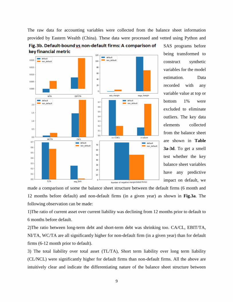
The raw data for accounting variables were collected from the balance sheet information
provided by Eastern Wealth (China). These data were processed and vetted using Python and
SAS programs before
being transformed to
construct synthetic
variables for the model
estimation. Data
recorded with any
variable value at top or
bottom 1% were
excluded to eliminate
outliers. The key data
elements collected
from the balance sheet
are shown in Table
3a-3d. To get a smell
test whether the key
balance sheet variables
have any predictive
impact on default, we
made a comparison of some the balance sheet structure between the default firms (6 month and
12 months before default) and non-default firms (in a given year) as shown in Fig.3a. The
following observation can be made:
1)The ratio of current asset over current liability was declining from 12 months prior to default to
6 months before default.
2)The ratio between long-term debt and short-term debt was shrinking too. CA/CL, EBIT/TA,
NI/TA, WC/TA are all significantly higher for non-default firm (in a given year) than for default
firms (6-12 month prior to default).
3) The total liability over total asset (TL/TA), Short term liability over long term liability
(CL/NCL) were significantly higher for default firms than non-default firms. All the above are
intuitively clear and indicate the differentiating nature of the balance sheet structure between
Page 10
10
risky firms and relatively healthy ones.
4)The relative profit margin (i.e. rela_margin = the firm specific profit margin relative to the
whole market ) is appreciably lower for default-bound than for non default firms (for the full
sample see Fig 3b
and for listed firm
sample See Fig 3c,
where the relative
margin at the
median for the
default-bound
firms is even worse
(negative) .
5) It is observed
that on average
during any given
period (“quarter“),
when there are
bond defaults, the
number and the
proportion of
money losing
companies are both
higher , compared to the periods when there is no default. This concurs with the intuition that
defaults is more likely to happen when the macro business condition is less benign.
6) For listed firms it is observed that: Relative Market Size, Equity Return (log return), Relative
Margin and Net Income and Cash as a percentage of market value of Total Asset, are all lower
for default-bound firms than non-default firms. These information provide intuitive support for
our empirical forecasting model based on balance sheet variables.
3. Empirical Methodology
Page 11
11
This section describes our econometric model using actual bond default data. In an attempt to
find the best approach to forecast the bond default, we will first estimate a few classic hazard
models using the same set of
variables as the original models
and then we will expand into our
own specification, which
incorporate several constructed
variables not traditionally used
in literature.
3.1 Model Specification
Since the seminal work of
Shumway (2001), the use of
hazard rate modeling technique (also called survival analysis) has become a standard
methodology in firm’s default prediction in developed market. The hazard rate is defined as the
conditional probability that an event of interest occurs within a particular time interval (t, t+ ),
given that it survived to the time t. Following Standard survival analysis literature (Klein and
Moeschberger, 1997), we define the hazard rate or intensity rate for the bankruptcy time , a
random variable, as:
Suppose we have collected a total sample data of N firms (i=1,…n), who listed their bond at the
bond market . Our observation period starts at the beginning (t=1) until the end (t=T) of our
sample period. However, the observation of any particular firm i continue from some starting
time ti (the start of its issuance of bond of first time) until sometime Ti < T when the firm
experiences bankruptcy ( i ) or is censored Ti. Censoring means that the firm is observed at the
time Ti but not at time Ti+1, Time Ti usually is the last date in our sample period. For example,
the firm could experience a merger and vanish from the data set. In this study, we ignore the
reoccurrence of default i.e. when a default occurred, the observation ends, even though it would
cure later before relapse. This process can be visually described by Fig.4. We define the discrete
time condition hazard rate process as:
for
i.e. The probability of default time occur between time period t and the following period (before
Page 12
12
censoring time )---given the fact that the firm survives to the period t-1, with corresponding time
dependent attributes where i is the discrete random variables giving the uncensored time of
event occurrence . It is also the conditional probability that an event occurs at time t, giving the
dynamic attributes. Following Chava and Jarrow (2004), we define:
i) the point process for this bankruptcy time as
ii) the random time Yi = min( i,Ti)
We estimated this probability via logistic link function
<2>
Where Xi,t-1 is a (k×l) vector of k
variables specific to firm i and lagged
one period, is a (
k ) vector of parameters, Z t-l is an
l×l vector of macro variables lagged
one period, is an vectors of
parameters, D is an m×l vector
dummy variables, corresponding firm’s
ownership type, sectors ,etc. t is a time
effect variable, representing the vintage
of the firm i. ɛit is assumed to be independently across firms.
3.2 Variable selection
The explanatory variables selected in the above discrete hazard model can be classified into three
categories: firm specific, macro level variables, and (equity) market related. Our basic criteria for
including covariates in the model is parsimoniousness, i.e. to develop a set of explaining
variables that provides the best differentiating power but not over fitting the data. In addition, the
variables selected must be numerically stable and conducive to out- of-sample test.
3.2.1 Balance Sheet Related, Firm Specific Variables
General features include age, ownership type dummy, and sector/industry dummies (defined in
4.2.4) according to the classification of Chinese Security and Exchange Committee. Individual
features include firm size, liquidity, profitability, and relative margin etc. Firm size is measured
Page 13
13
as the ratio between the firm’s revenue over industry median as a measure of firm size. Relative
size refers to the ratio between firm revenue over total revenue of all firms within the same sector.
We choose the relative size because it reflects the dynamic status market share of the firm. If it
loses competitiveness to its peers, this measure will reflect that and its credit risk would increase.
Liquidity is measured by a) CACL, current asset/current Liability, b) TATL, total asset/total
liability and c) CLCNL: short term debt/long term debt. Profitability: is measure as: a) RETA,
ratio of retained earnings (RE) vs total asset. b) Relative margin is a key measure of firm’s
pricing power and strength. The lower margin, the less the pricing power of a firm. We use profit
margin relative to sector median (rela_margin) to measure the competitiveness of the firm. A
rough glance of Fig.5 shows the medium of relative margin of default companies is much
smaller than that in healthy companies. EBIT over total asset (EBIT/TA) and Net Income over
Total Asset (NITA) are measures of return on asset. Other computed variables include: ii) Z-
score, a widely used indicator to discern “unhealthy” firm from healthy ones. We computed the
Chinese version of Z-score developed by Altman (2007); 2) Negative DVX [ln(1-RE/TA)], an
indicator used by IMF paper, to capture the potential asymmetric effects of positive and negative
retained earnings. It is the negative dummy variable.
It is expected that the sign of the estimated coefficient to be negative in our setting, meaning a
positive RE will reduce the probability of default. 7
3.2.2 Altman Z score: A Synthetic Measure of Financial Health of Firm with accounting
variables
Altman (1968)’s Z score has been proved to be an effective discriminator for corporate default
risk and is still a widely used gauge for firm’s financial health in US and developed countries
(albeit with variations adjusted for countries). Working with several prominent researchers in
China, Altman (2007) established a Chinese version of Z score and applied it to diagnose
potential distress of Chinese firms. Based upon our literature search, however, it has never been
empirically tested against actual default experience due to the lack of occurrence until recent
years (the same reason that accounting based models were almost non-existent in academia for
7 According to the Authors, this additional variable is to account for a peculiarity in China—retained earnings were
negative for about one-fifth of sample observations. This fact was independently confirmed by us.
Page 14
14
China market, as discussed in the Introduction). To fill this literature vacuum, we tested its
validity in this paper. We first computed Altman’s Z-score for Chinese firm, as a composite
measure of default risk implied in the financial ratio, using Altman’s original coefficients
( henceforth “Altman ZChina
“) and then we re-estimated the Z-Score (with Linear
Discriminatory Analysis) using the same set of
variables (henceforth “Test- Z-score”), i.e. Total Liability/ Total Asset, : net Profit/Total asset,
working Capital/Total assets, : Retained earnings /Total asset).
Note that all the variables have correct and interpretable sign (the sign of RETA in the original
Altman ZChina
score is unintuitive.
3.2.3 Macro variables
It can be argued that the macroeconomic environment significantly affects the default. There are
numerous candidates for the macro variables, such as change in exchange rate, GDP growth,
unemployment rate, global liquidity etc. Given the relatively short period of time horizon since
the first actual bond default, these variables are not collected across economic cycles and thus
not sensitive enough to have meaningful impact on the quarterly default events in China.
Therefore, in the spirit of parsimony, we constructed a proxy to characterize the general business
conditions under which the bond issuers are operating: nega_margin, which is defined as the
proportion of firms with negative profit margin among all bond issuers for the same period. The
less the number, the better the credit environment. Using this proxy as macro variable can be
justified by the fact that under a distressed economic condition, there would be much more firms
that operate at loss. Since the sample we collected covers the bond-issuing firms quite broadly—
in terms of size, geographical, ownership type and industry, we assume that the proxy is
representative of the economy as whole.
3.2.4 Market Variables
For Listed companies, we constructed following variables of equity market.
1) ME/TL =Market Cap over Total Liability
This is the measure of dynamic leverage, with market cap supposedly reflecting the latest
information about the investor’s expectation of the firm’s future free cash flow, the large the
ratio, the less the leverage of the firm, which should correspond to less default risk.
Page 15
15
2) Relative Return: log_return
It is defined as Rela_Return = Ri /R
market , Where R
i and R
market stand for quarterly log return for
firm i and the overall market respectively. The “overall market” is embodied by the Index of the
Shanghai Stock Exchange. This is a measure of the risky equity return (quarterly) relative to the
broad market. Breig at el (2009) summarized four compelling argument why equity return and
default risk are negatively correlated. To the degree the equity market is efficient, the stock
price contains certain timely information about the credit quality of the issuer.
3) Relative Market Size RSIZE = Firm’s Market Cap i /Market Cap
China Market
This is a measure of relative importance of the firm in terms of the market cap. In general, the
larger the relative size valuated by the equity market, the less probable it will default since its
asset is valued higher than its liability by the market. To the degree that a firm’s equity position
is weak, its asset value is close to its debt. Therefore, we expect a negative sign of this variable.
4) Net income, Cash and Total Liability as percentage of market value of total asset:
NIMTA = Net Income / Market Value of Total Asset
CASHMTA= CASH/ Market Value of Total Asset,
TLMTA = Total Liability/Market Value of Total Asset
where Market Value of Total Asset ≈ Equity Market cap + Book Value of Debt
5) Distance to Default
Essentially, DD is a measure of the difference between the asset value of the firm and the face
value of its debt, normalized by the standard deviation of the firm’s asset value. To implement
the structural approach, the calculation was done in the manner of Hillegeist et al. (2004) by
solving a system of two nonlinear equations.
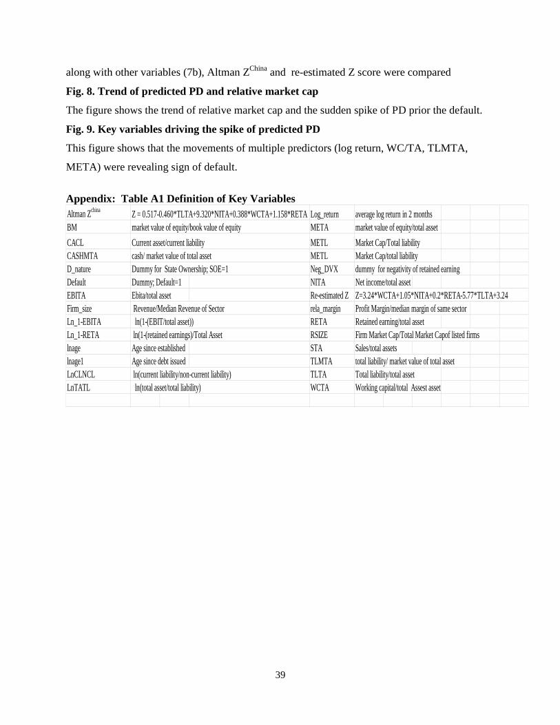
All the key variables are listed in Appendix Table A1.
3.3 Model Performance Measure
To gauge the performance of risk classification of the model, we rely on Pseudo-R2 and the
Receiver Operating Characteristics (ROC) (also used by Chava and Jarrow (2004) as a measure
of a model's ability to discriminate between bankrupt and non-bankrupt firms. AUROC is the
area under the ROC curve, and a larger area indicates that the model is correctly predicting more
bankrupt firm as being likely to fail. Its value ranges between 0.5, indicating no discriminatory
power, and 1, implying perfect identification of bankrupt and healthy firm. In general, there is no
Page 16
16
‘golden rule’ regarding the value of AUROC, however anything between 0.7 and 0.8 is
acceptable, while above 0.8 is considered to be excellent (Hosmer Jr et al. 2013).
4. Results and Analysis
In this section, we provided our estimation results of the models described in 4.1. We estimated
the following models using the default data available and compared their performance.
4.1. Hazard Model with Merton implied PD vs Actual Default event
Recall that the IMF’s paper linked a set of balance sheet (financial ratios) to the market-implied
PD (converted from risk neutral PD) as the dependent variable in a logistic formulation. To test
the validity of this approach, we used the same set of variables to estimate a discrete hazard
model with actual default data for listed
companies. The results are shown in Fig 6.
The results indicate that all empirical
models outperform IMF Merton model in
terms of predictive power of default
probability. We attribute this weak
performance of the model to several
deficiencies of this approach applied to
Chinese market. Firstly, the Chinese
equity market is grossly over-valued by
any measure and the unobserved “Firm value” could be significantly over estimated, resulted in
low probability of default. Secondly, in adjusting the risk neutral to actual PD, the risk neutral
PD were fitted on approximation of Moody’s proprietary database of actual default rates. This
database, however, includes only North American firms which “operate in a very different
economic and legal environment to Chinese firms. Bankruptcy procedures in the United States
and Canada are well defined, tested through the economic cycle, and rarely influenced by actual
or prospective public sector bail-outs. These conditions do not yet hold for China. Moreover, to
convert the risk free-rate was convert risk-neutral to actual default probabilities, the risk free-rate
in Merton model was replaced by a drift term that was designed to capture the time-varying price
of risk and was calculated as the product of the correlation between the equity price of the firm
and the market and the ex-post Sharpe ratio, and this ratio, however, had been anti-intuitively
Page 17
17
close to zero or negative during 2008 to 2013. The authors thus used the “theoretically-consistent
prior” but did not elaborate how this was done. Lastly, while the Merton implied Probability of
Default is converted to empirical PD, there was no default data to validate whether these PD
have discriminating power.
4.2. Testing classic default forecasting models using bond default data of China
To see if the classical empirical models in the literature, which have been well tested in the
developed market such as US, are still applicable in China market, we re-estimated some of the
well-cited forecasting models, such as Shumay (2001) and Zmijewski (1984). In general, our results
are similar to those studies in US markets. As in the literature, the default probability is
associated with small firm size, low net income to total assets, low current asset to current
liability, and low working capital to total assets. Of all the default-forecasting studies, Shumway
(2001) is a milestone. Shumway's main contribution was to estimate a hazard model, which
enabled him to use all available information to determine each firm's bankruptcy risk at each
point in time". This improves the static logit model (before his seminal paper) in that it includes
all firm-years as observations instead of only one firm-year for each firm. Specifically, the author
Table 7 Shumway’s’ Hazard model on US firms vs Our re-estimates using China Data
Model/Coefficient WC/TA RE/TA EBIT/TA ME/TL Sale/TA Ln(age) Intercep
t
( p-value )
Shumway(2001), -0.732 -0.818 -0.8946** -0.1712** 0.158 0.015 -3.226**
Table 2/Panel B., -(0.577) -(0.312) -(0.001) -(0.012) -(0.446) -(0.967) -(0.001)
p117
Re-estimates using -4.1566 -9.5814 -22.1791 0.3305 -1.3144 1.252 -8.5281
latest default (0.006) (0.007) (0.167) (0.001) (0.349) (0.278) (0.014)
data(Table 9
below)
(henceforth "PJW")
Both having Both having Both having Both are Both are Both
correct sign correct sign correct sign significant insignificant model are
but PW but PJW but Shumway but while insignificant
model is model is model is PJW has PJW
more more more wrong has wrong
plausible plausible plausible sign sign
from p-value from p-value from p-value
perspective perspective perspective
Page 18
18
uses a dataset of non-financial firms that began trading between 1962 and 1992 on either NYSE
or AMEX. The resulting dataset contains 300 bankruptcies among 3,182 firms and 39,745 firm-
years. The dependent variable is set to 1 when the firm goes bankrupt and to 0 otherwise. We re-
estimated Shumway’s model with the data set described in 2.2. The comparison of Shumway’s’
Hazard model on US firms vs our estimates using China’s data are shown in Table 7, where it
can be seen that our estimates have the same (correct) sign and are statistically significant at 1%
for ME/TL and EBIT/TA, as well as the intercept For WC/TA; both have the same correct sign
but our model looks slightly more plausible judging from p-value perspective . For the rest two
variables Sale/TA and Ln (age1), none of two estimates is both correctly signed and significant.
In the Zmijewski’s paper (1984), three most common determinants, net income to total assets,
total debt to total assets, and current assets to current liabilities were included. Higher leverage
(TL/TA) and lower return on assets (NI/TA) are associated with a higher probability of default,
while the relationship between liquidity (CA/CL) and default risk is not statistically significant
(as re-estimated by Shumway 2001, Panel A, Table IV). By comparison, our results (Table 10b),
show that, when all the above variables were included in the model, both the liquidity and return
on assets have the correct sign and significant; but the leverage (TL/TA) does not have the
intuitively interpretable sign. We reasoned that since TL/TA is associated with long term
debt/short term debt, high TL/TA firms are more likely to have higher ratio of long term debt 8 ,
which could serve as some degree of mitigation for liquidity stress and default. Econometrically,
this implies there is some co-linearity between TL/TA and CA/CL9. This can also be seen from
the results summarized in Table 10b, where both NI/TA and CA/CL have expected sign and are
significant when TL/TA is taken out of the model specification.
Role of State Own firm
Given the data, it is interesting to note that State Own Entity (SOE) is less prone to
default as indicated by the negative sign of d_Nature, whose value is set to 1 if the firm is a
State-Owned. Note that this result contradicts to the IMF paper, where coefficients for both local
and central SOE have statistically significant positive sign (Table 9 in IMF paper), implying that
being a SOE is more likely to default. We believe our results are more plausible for the following
8 Based upon the balance sheet data from WIND, it was found that the correlation between TL/TA and Long term
debt/Short term debt is statistically 0.2208 (p=0.0002);. And the median ratio of long term debt/Short term debt is
0.35 for defaulted firms (one year before default) as compared to 0.45 for non defaulted firm. 9 The Pearson correlation between TL/TA and CA/CL was found to be statistically significant -0.16.
Page 19
19
reasons. First, the leverage ratios for state-owned firms are low, a fact that was empirically tested
by Wang (2013) from Tsinghua University10
. Secondly, an SOE usually enjoys funding
advantage over private firms, particularly when it comes to restructuring if in distress. Therefore,
an all-out default was usually avoided. Further, In China, SOE bonds are widely deemed as fully
guaranteed by the government and the issuers are usually bailed out when in financial distress.
Therefore, the SOE bonds could be issued at lower yields versus private company bonds. Those
bonds were allowed to default by regulator in 2015 to relieve the government from the role of the
government, especially local government, treats SOEs differently. Some SOEs have a closer
relationship with local government than others. Local government is inclined to bail out those
enterprises that it deems important, such as those that contribute more employment and tax
revenue.
Our findings are consistent with some literature on default in emerging market. For
example, in a similar study on corporate default of Jordan, Zeitun and Tian (2007) suggested that
government ownership was significantly negatively related to the firm's probability of default.11
In IMF paper, however, it implied that local SOEs are more prone to default. We thus conclude
that some results from the IMF paper are not convincing, nor are they consistent with the actual
default data so far. We believe, this result is likely generated by distorted market parameter. One
is magnified volatility. Large blocks of stock in state-owned enterprises do not trade as they are
held by government entities. It is the restricted shares that reduced the liquidity of SOE and thus
contributed to heightened volatility of equity market, which in turn would magnify the asset
volatility. Higher volatility will reduce the model calculated “Distance to Default”, resulted in
higher default probability derived for SOE12
..The other is uncertainty in Liability Estimation.
10
The university is often dubbed as “China’s MIT”. 11
Their paper “Does ownership affect a firm's performance and default risk in Jordan? “ was extracted from
http://ro.uow.edu.au/cgi/viewcontent.cgi?article=2516&context=commpapers 12
This can be seen from the basic version of Merton’s Model :
Prob (Default) = )( DD
Where (.) denote the cumulative standard normal distribution, and DD denotes “distance to default”, defined as:
tT
LtTrVDD
t
t
ln))(2/(ln 2 ,where tV is the (unobserved) firm value, v is the volatility of firm’s asset value,
which follows a geometric Brown process, L is the total liability of the firm. See for example, p29, “Credit Risk Modeling Using
Excel and VBA , Gunter Loffler, Peter N Posch, 2014
Page 20
20
One of the key parameters of Merton model is the book value of liability as the barrier of default.
The true liability is hard to gauge for state owned firms since they usually can get soft funding
and even “debt forgiveness” due to their relationship with the government. The two combined
could lead to wrong conclusion applying Merton’s model to China’s equity market to establish a
causal relationship between the ownership structure and the derived PD. There are several key
explanatory variables that are supposedly contributing to the default.
The Role of Market Variables
Theoretically, it is expected that the informed investor will discount the default risk by lowing
the stock price so that the return from investing the equity underperform the market; The firm
with higher leverage (associated with lower equity value) should be more likely in distress and
thus prone to default. In addition, if all the market variables included in this estimation
incorporate all the default signals contained in the quarterly accounting reports, then the forecast
should outperform the accounting based. To test this concept, as was done similarly in Shumway
(2001) and Jarrow (2004), we estimated the model with specification that excludes the
accounting variables and the results are shown in Table 10a. The simple model with only
Distance to Default has the lowest differentiating power in terms of AUC (0.52) and AIC
(highest) with insignificant coefficient, albeit with correct sign (i.e negative)---even the simple
model with univariate of Log_Return performs much better, fetching a 0.76 AUC (than model
DD performs worse than the Adding other market variables including relative log-Return
improves the model performance , albeit slightly. The model with labeled (“DD & Return”) is a
simple model incorporating only the log equity return and DD but shows decent predictive power
(with AUC being 79%, beating other alternatives in the table. Model 2 and Model 3 contains not
only all the available market related variables , but also the business condition indicator (i.e.,
nega_margin) and relative profitability measure , i.e. relative margin; both outperform Model
1 which does not incorporate these two additional variables (In fact Model one has the second
lowest AUC). It is observed, however, the relative equity value (MV/BV, ME/TA) is neither
insignificant nor correctly signed (Model 2, which exclude Distance To Default , has expected
negative sign of MV/BV but insignificant ). This indicate that the relative value placed on the
Page 21
21
firm’s equity by stockholder is not a good discriminatory for default risk. Recall that in Fig 3b,
it was shown that the average market-to-book ratio default-bound firm is almost the same as non-
default firm. Apparently, there is an overvaluation of the equity market which underestimates of
default risk by equity holders. Interestingly, this result coincides with Campbell (2008) a well
cited paper, which studies US market. Campbell (2008) noted that that “the average market-to-
book ratio is slightly higher for bankruptcy “and the variable is insignificant, with the wrong sign
(Table IV, p2913); In Law and Roache (2015) in its comprehensive study on China firm default,
using the Merton’ implied PD as the dependent variable, found that the Market/Book ratio
significant but had a wrong sign. In a recent study by Cerrato et al (2016) on default for listed
Chinese firm, it was reported that market-to-book is a significant predictor with the expected
sign (Table 5); however, some other key explanatory variable, such as NI is neither significant
nor have correct sign and the overall out of sample fitting is poor (AUC =0.67) . In general,
default firms often experience losses and these depreciate the book value of their equity; thereby
the market-to-book ratio rises up. On the other hand, investors’ s informed default risk may
could weigh on the equity value and the market-to-book ratio. The ending result is depends upon
which side dominate. In China’s market, it is well likely that investors were kept in the dark
until the last minute.
As is well known, the quality of financial disclosure for many Chinese companies are
notoriously poor. Even the for the listed companies and/or bond issuers, the financial statement is
not up to the standard of West. Under these circumstances, the collective intelligence of equity
market might somehow help remedy the deficiencies of accounting variables in signaling default
risk. We will demonstrate this point in a more concrete way in a case study at the end.
Table 10a Simple Hazard Models with market variables only This table exhibits the estimation results and predictive power for several selected models that incorporate
only market-related variables, one of being the Distance to Default, an indicator for default risk,
calculated under Merton’s structural model framework. This table is to test the differentiating power of
the market variables alone without the auxiliary of any accounting variables. These models were
estimated with the sub sample of listed companies, which included a relatively small number of defaults
(18 in total). The p-values were reported in parenthesis. * denotes significance at 5%, ** denote
significance at 1%. The overall out of sample predictive power of each model is gauged by AUC and AIC
listed in the last two rows of the table.
Page 22
22
That the Distance To Default under Merton‘s framework exhibits very poor discriminating
capability does not means market variables are not useful at all. In fact, given the limited sample
size, the properly selected market variables could save the day for accounting variables. This
can be seen from Table 10b, if only the sample of listed companies are used to train the model
with the balance sheet /accounting variables (e.g Zmijewski or Shumway ) the predictive
power of the model is very weak, with a paltry AUC of 0.55, implying the model almost no
better than a random classifier. However, when several market variables such as log_return (i.e.
firm’s quarterly return relative to the whole market) and NIMTA, the performance is
significantly improved.
Table 10a Hazard Model with Market Variables Only
Variables naïve_dd log_return dd&return dd/return/margin dd/return/rela_margin model
1
model
2
model
3
Intercept -6.727 -7.2959 -7.2629 -6.275 -6.988 -6.149 -7.2806 -
12.9188
0 0 0 0 0 0.043 0.023 0.005
naive_dd -0.0018
-0.0011 -0.001 -0.0011 -0.0004
0.0003
0.681
0.728 0.755 0.709 0.906
0.921
CASHMTA
-15.412 -13.89 -15.30
0.02 0.03 0.02
Lnage
-0.067 0.1162 1.9219
0.943 0.908 0.194
BM
(=MV/BV ) 0.038 -0.2365 0.018
0.808 0.3 0.937
NIMTA
-133.1 -110.79 -12.77
0 0 0.817
TLMTA
2.0162 1.9452 2.9153
0.24 0.26 0.128
META
0.311 0.4234 0.7973
0.373 0.231 0.203
log_return
-3.753 -3.7236 -3.4902 -3.4094
-2.9616 -3.4848
0 0 0 0
0 0
nega_margin
-2.5208
-2.066
0.652
0.715
rela_margin
-0.2849 -0.2483
-0.2408
0.008 0.033
0.194
AUC 0.52 0.76 0.79 0.71 0.72 0.62 0.71 0.73
AIC 283.22 257.4 224.15 259.34 260.07 274.91 259.98 258.66
Page 23
23
Table 10b Classic Hazard Models Trained with Sample of only Listed Companies This table reports the predictive power and coefficients estimated from the sub sample of listed
companies for several classic hazard models predicting defaults in developed market such as US. The
sub -sample included a relatively small number of defaults (18). For each model, we first estimated the
original version and then expanded the model by incorporating some new variables related to the equity
market. The predictive power of the expanded model was compared with the original one’s. This is to
demonstrate that while Distance to Default (under Merton’s framework) provides little predictive power,
certain equity market related variables do contain additional information about default risk when the
accounting variables are s rendered powerless by the relatively small data sample of listed companies. *
denotes significance at 5%, ** denote significance at 1%.
Table 10b Classic Models Trained with Sub Sample of Listed Companies
Variables zmijewski zmijewski_mkt shumway shumway_mkt IMF IMF_mkt
Intercept -7.3329 -6.7058* -4.8904 -4.9752 -0.314 -1.2042
(0.011) (0.027) (0.076) (0.086) (0.936) (0.769)
log_return
-2.7964**
-3.0354
-3.4996
(0.000)
(0.000)
(0.000)
CASHMTA
-15.2868**
-14.8407
-11.8913
(0.013)
(0.014)
(0.051)
Naïve_DD
NIMTA
-102.6028**
(0.000)
Lnage -0.4107 -0.1126 -0.0342 0.1798 -
0.5288 -0.1709
(0.616) (0.907) (0.971) (0.852) (0.620) (0.873)
TLTA 3.6725 2.7492
(0.056) (0.144)
CACL -0.0983 -0.0699
(0.785) (0.844)
NITA -64.0792
(0.001)
WC/TA
-1.8423 -1.1407 -0.822 0.3465
(0.113) (0.340) (0.512) (0.778)
S/TA
-1.8815 -1.1594
(0.185) (0.361)
EBIT/TA
-17.824 -14.9953
(0.247) (0.317)
RE/TA
-7.5202 -6.6392
(0.004) (0.071)
Ln_1-
EBIT/TA -43.88 -47.82
(0.004) (0.001)
Ln_1-
RE/TA -4.126 -6.748
(0.308) (0.026)
Page 24
24
neg_DVX
4.1017 4.4702
(0.000) (0.000)
LnTATL
-3.989 -4.2483
(0.008) (0.009)
Ln_CLNCL
-0.138 -0.0917
(0.323) (0.562)
firm_size
-0.163 -0.0934
(0.071) (0.247)
AUC 0.52 0.73 0.55 0.76 0.75 0.83
AIC 275.65 236.69 267.2 227.98 235 218.78
Table 11 Classic Hazard Model Trained with the full sample This table reports the estimation results (and out of sample performance) for several classic models
(including one, i.e. IMF model developed specifically for China market). These models were re-estimated
with the full data sample. For each model, we first estimated the original version using accounting
variables only and then expanded the model by incorporating two additional variables we deem
informative in predicting bond default: one is relative_margin, a measure of firm’s profitability of the
firm relative to the overall market, the other is quarterly business condition index, measured by the
proportion of firm that lose money in the quarter. The predictive power of the expanded model was
compared with the original one’s. This is to demonstrate that while Distance to Default (under Merton’s
framework) provides, certain variables related equity market do contain additional information in
predicting bond default when the accounting variables are powerless rendered by the small data sample
limited to listed companies. * denotes significance at 5%, ** denote significance at 1%.
Table 11 Hazard Model Estimated with Full Sample Using Accounting and Macro Variables
Variables zmij
ewsk
i
zm
ijew
ski_
wit
h m
acr
o
an
d r
elati
ve
marg
in
vari
ab
le
shu
mw
ay
sh
um
wa
y_w
ith
macr
o
& r
elati
ve
marg
in
IMF
's
Ch
ina
Def
au
lt M
od
el
IMF
_w
ith
macr
o
vari
ab
le
IMF
Mo
del
Vari
ati
on
1
IMF
Mo
del
Vari
ati
on
2
Ou
r p
rop
ose
d
Bes
t
Per
form
ing M
od
el
Intercept -10.45 -8.78 -6.91 -6.87 -0.91 -2.68 -2.05 -2.94 -7.28
0.00 0.00 0.00 0.00 0.57 0.11 0.18 0.06 0.00
d_nature
-2.29
-2.21
-2.14
-2.35 -2.32
0.00
0.00
0.00
0.00 0.00
firm_size
0.00
0.00 -0.01 0.00 -0.01 0.00
0.67
0.96 0.40 0.85 0.57 0.86
nega_margin
4.27
1.41
3.03
2.56 5.22
0.03
0.46
0.14
0.21 0.01
rela_margin
-0.46
-0.57
-0.69
-0.45 -0.46
Page 25
25
0.00
0.00
0.00
0.00 0.00
Lnage 0.56 0.45 0.62 0.43 0.31 0.36 0.30 0.37
0.09 0.21 0.07 0.24 0.37 0.34 0.39 0.32
TLTA -18.27 4.32
1.07
0.00 0.00
0.42
CACL 5.92 -0.14
0.02 0.37
NITA -0.37 8.04
-149.17
0.05 0.28
0.00
WC/TA
-3.60 -2.82 -1.94 -1.76 -2.01 -2.40 -1.58
0.00 0.00 0.01 0.03 0.00 0.00 0.04
S/TA
0.51 0.24
0.02 0.40
EBIT/TA
-21.00 -6.30
-16.03 -7.94
0.00 0.05
0.00 0.04
RE/TA
2.53 6.99
11.08 10.64
0.18 0.01
0.00 0.00
Ln_1-EBIT/TA
-1.21 -45.34
-180.79
0.89 0.00
0.00
Ln_1-RE/TA
-10.52 -10.71
0.00 0.00
neg_DVX
3.74 4.05 3.52 3.76 2.97
0.00 0.00 0.00 0.00 0.00
LnTATL
-4.76 -3.33 -3.63 -2.57
0.00 0.00 0.00 0.00
Ln_CLNCL
0.26 0.06 0.31 0.001
0.06 0.68 0.02 0.98
AUC 0.69 0.82 0.65 0.81 0.80 0.87 0.78 0.86 0.91
AIC 910.87 800.29 925.65 800.52 831.31 705.27 838.56 739.06 659.25
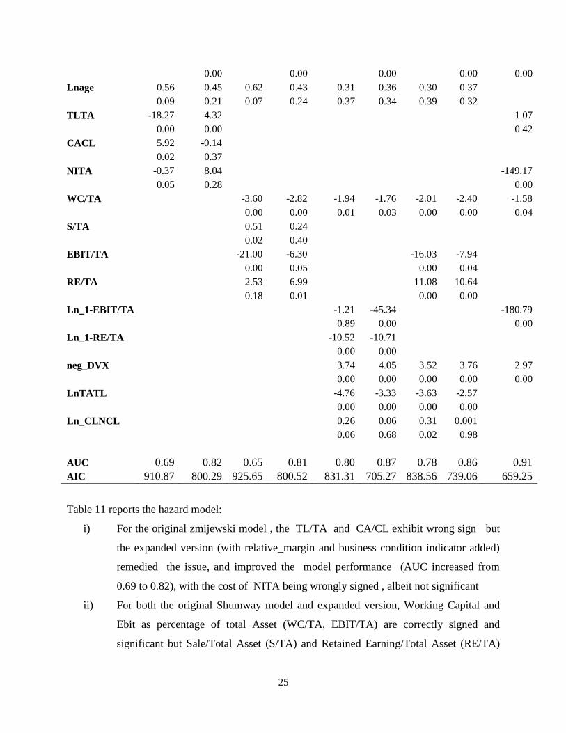
Table 11 reports the hazard model:
i) For the original zmijewski model , the TL/TA and CA/CL exhibit wrong sign but
the expanded version (with relative_margin and business condition indicator added)
remedied the issue, and improved the model performance (AUC increased from
0.69 to 0.82), with the cost of NITA being wrongly signed , albeit not significant
ii) For both the original Shumway model and expanded version, Working Capital and
Ebit as percentage of total Asset (WC/TA, EBIT/TA) are correctly signed and
significant but Sale/Total Asset (S/TA) and Retained Earning/Total Asset (RE/TA)
Page 26
26
are not. The expanded version, though, significantly enhanced the model performance
(with AUC increased from 0.65 to 0.81)
iii) Re-estimated original IMF model using actual default rather than using Merton model
implied PD as independent variable exhibit quite good out of sample performance
(with AUC being above 0.80), all but two log transformed variable (1-EBIT/TA) and
(1-RE/TA) have incorrect sign. This problem is remedied once the log transformation
is removed in the variance versions;
iv) The negativity (flag neg_DVX) for retained earning has correct sign and significant.
When a company records a profit, the amount of the profit, less any dividends paid to
stockholders, is recorded in retained earnings, which is an equity account. When a
company records a loss, this too is recorded in retained earnings. If the amount of the
loss exceeds the amount of profit previously recorded in the retained earnings account
as beginning retained earnings, then a company is said to have negative retained
earnings. Negative retained earnings can arise for a profitable company if it
distributes dividends that are, in aggregate, greater than the total amount of its
earnings since the foundation of the company. It is observed that the number of firms
with negative retained earnings is disproportionally high (23% for firms lurching
towards default vs 3% of all sample population. Negative retained earnings appear as
a debit balance in the retained earnings account, rather than the credit balance that
normally appears for a profitable corporation. On the company's balance sheet,
negative retained earnings are usually described in a separate line item as an
"Accumulated Deficit." Indeed, the variable used to flag the negativity of the retained
earnings, neg_DVX shows correct sign and is significant.
v) Both the relative profitability proxy (rela_margin) and the business condition proxy
(nega_margin) are significant and correctly signed cross all model specifications, so
is the ownership nature flag: d_nature.
Table 12 Best Performing Hazard Models
This table takes our best -model variables for listed firm sub-sample and full sample and report their
statistical significance and predictive power. The dependent variable is bond official default. The
explanatory variables are selected by an optimal process via Lasso regression. The P-value is reported in
parentheses. * denotes significance at 5%, ** denote significance at 1%.
Page 27
27
Table 12 Best Performing Models Selected by Lasso Regression Process
M
1:
Hy
bri
d_m
od
el
tra
ined
wit
h l
iste
d
sam
ple
M2
:
tra
ined
wit
h
full
sam
ple
M3
: tr
ain
ed w
ith
list
ed s
am
ple
M4
:
tra
ined
wit
h f
ull
sam
ple
M5
: w
ith
re-
esti
mate
d Z
incl
ud
ed
M6
: w
ith
Alt
ma
n
ZC
hin
a in
clu
ded
Intercept -14.8723** -7.28* -8.22** -6.7107 -2.5719 -4.699
0 0 0 0 0.078 0.001
WC/TA -4.4139 -1.577 -1.9634 -1.7438
0.022 0.041 0.214 0.015
rela_margin -0.5734 -0.455 -0.2595 -0.4124 -0.221 -0.21
0.003 0 0.029 0 0.00012 0.00015
EBIT/TA
7.2082 -9.22
0.653 0.257
Ln_1-
EBIT/TA -285.037 -180.8
0 0
TLMTA 5.3068
0.6837
0.005
0.645
NIMTA -308.8708
-23.0674
0
0.758
CASHMTA -16.1289
-13.1437
0.029
0.065
log_return -3.8939
-3.3969
0
0
ln_rela_size -0.6076
-0.3747
0.0025 -0.1904
0.011
0.064
0.983 0.091
neg_DVX
2.9728
2.6944
0
0
d_nature
-2.317
-2.6292 -2.2128 -2.487
0
0 0.0002 0.00036
nega_margin 5.2187
3.0829 0.0085 0.01
0.01
0.145 0.00017 0.0027
TLTA
1.0748
3.2245
0.422
0.008
NITA
-149.2
27.409
0
0.033
lange1
-0.1134 -0.1194
0.493 0.464
Page 28
28
Lage
0.2788 0.4098
0.493 0.246
Re-estimated Z
-0.6793
0.0003
Altman
ZChina
-1.79
0.001
AUC 0.856 0.91 0.75 0.84 0.87 0.838
Following Hardle (2103), we employed a unified regularization approach (LASSO) , with logit
as an underlying model, which simultaneously selects the default predictors and optimizes all
the parameters within the model. The LASSO is a regularization technique for simultaneous
estimation and variable selection, now widely used for model selection in machine learning
algorithm and has been recently introduced into corporate bankruptcy forecast (See Tian, etc.
2015 for an excellent discussion about the advantage of using LASSO regression to improve in-
sample and out of sample performance). K-fold cross validation was used to validate these
models.
The coefficients of the selected variables are reported in Table 12. These models are
characterized by i) Good out-of-sample performance measured by AUC (most of the greater than
80%.) ii) Almost all coefficients are significant with at most one exception iii) Correctly signs of
the coefficients. The first two models have the best out-of- sample predictive power; All but one
coefficient (ln (1-EBIT/TA), are correctly signed and statistically significant. Further it can be
seen from table 12 that: 1) Working Capital as percentage of total asset, WC/TA, Relative
profitability measure (relative_margin) and log return are all significant and have correct sign
across all the best models. In particular, both Altman’s original Chinese Z score and our re-
estimated Z score (using the same variables). Models trained with the sub sample of listed
companies underperform those trained with the full sample in terms of out of sample predictive
power measure by AUC. This is understandable since there has been relatively smaller number
of the listed companies that experienced bond default and the estimation results may not be
robust. As we demonstrated in Table 10b, however, market variables do add information value
to predictive power on top of accounting variables given the fact that a model incorporating only
accounting variables but trained with the sub sample of listed companies would perform much
worse.
3. Role of firm size
Page 29
29
With regard to the role of firm size, our results are not totally in line with other studies, such
as Ohlson's (1980), whose results showed that corporate default is associated with small firm size.
In our case, the firm size measured by revenue has either wrong size or insignificant (Table 11).
Liquidity
In the seminal paper of Shumway (2001) and paper of Zmijewski (1984) as well, both TL/TA
and CA/CL were included. While the expected signs of the coefficients were obtained (positive
for TL/TA and negative for CA/CL), one of the coefficients (i.e. CA/CL) was not significant
(Shumway 2001, Table II, Panel A).
Age
Our estimation results show that older firms measured by age (defined in Section data and
Variable selection) have higher propensity to default, as evidenced by the fact that the sign of Ln
(Age) are positive and statistically significant across all specifications. This result is in line with
Shumway (2001) hazard model estimate (Table II, Panel B) and Jarrow (2004) re-estimated
Zmijewski (1984) and Altman (1968) z-score variable set using US data from 1962-99. We
noted that the result on this variate is also in line with the IMF model, the only model that
contains statistically significant coefficient for the age is Model 5; and the sign is positive as
reflected as pooled regression on market implied PD in IMF paper, Table 11, Model# 5. The
sign and significance remain robust even if the regression is done with or without SOE firms
excluded.
4.3 Test Altman’s Chinese version Z-Score
Page 30
30
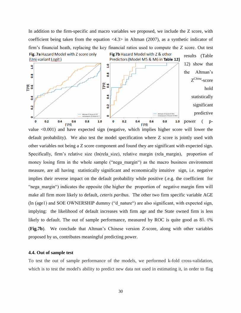
In addition to the firm-specific and macro variables we proposed, we include the Z score, with
coefficient being taken from the equation <4.3> in Altman (2007), as a synthetic indicator of
firm’s financial heath, replacing the key financial ratios used to compute the Z score. Out test
results (Table
12) show that
the Altman’s
ZChina
-score
hold
statistically
significant
predictive
power ( p-
value <0.001) and have expected sign (negative, which implies higher score will lower the
default probability). We also test the model specification where Z score is jointly used with
other variables not being a Z score component and found they are significant with expected sign.
Specifically, firm’s relative size (ln(rela_size), relative margin (rela_margin), proportion of
money losing firm in the whole sample (“nega_margin“) as the macro business environment
measure, are all having statistically significant and economically intuitive sign, i.e. negative
implies their reverse impact on the default probability while positive (.e.g. the coefficient for
“nega_margin“) indicates the opposite (the higher the proportion of negative margin firm will
make all firm more likely to default, ceteris paribus. The other two firm specific variable AGE
(ln (age1) and SOE OWNERSHIP dummy (“d_nature“) are also significant, with expected sign,
implying: the likelihood of default increases with firm age and the State owned firm is less
likely to default. The out of sample performance, measured by ROC is quite good as 85.4%
(Fig.7b). We conclude that Altman’s Chinese version Z-score, along with other variables
proposed by us, contributes meaningful predicting power.
4.4. Out of sample test
To test the out of sample performance of the models, we performed k-fold cross-validation,
which is to test the model's ability to predict new data not used in estimating it, in order to flag
Page 31
31
problems like overfitting or selection bias13
. In this procedure, we first divide the training
dataset into 5 folds. For a given hyperparameter setting, each of the 5 folds takes turns being the
hold-out validation set; our hazard model is trained on the rest of the 4 folds and measured on the
held-out fold. The overall performance is taken to be the average of the performance on all 5
folds. Repeat this procedure for all of the hyperparameter settings that need to be evaluated, then
pick the hyperparameters that resulted in the highest 5-fold average. here is a bias-variance
trade-off associated with the choice of k. Given our limited default data set, we choose k = 5 for
overall dataset, k=3 for listed firms, as this parameter empirically yield test error rate estimates
that suffer neither from excessively high bias nor from very high variance. Although we cannot
test model performance from k=10, we randomly split overall data and run k-fold cross-
validation more than 3 times. All our performance measure (AUC) reported in Table 10-12 are
the average results generated from this out of sample test.
5. Case Studies
With the general results discussed above, we are presenting here some case studies to provide a
concrete demonstration how the
model performs for individual firms
and to highlight the difference
between our proposed approach and
the previously dominant methodology
represented by the IMF paper. We
compared the time series of PD
estimated by different models and check
how well the forecasts were borne out by
actual default events. All the cases are
out-of-sample firms.
13
In the k-fold cross-validation, the original sample is randomly partitioned into k equal sized subsamples.
Of the k subsamples, a single subsample is retained as the validation data for testing the model, and the
remaining k − 1 subsamples are used as training data. The cross-validation process is then
repeated k times, with each of the k subsamples used exactly once as the validation data. The k results can
then be averaged to produce a single estimation. The advantage of this method over repeated random sub-
sampling (see below) is that all observations are used for both training and validation, and each
observation is used for validation exactly once.
Page 32
32
5.1. The sudden default of Kangde Xin Composite Material Group Co. (01/15 2019 default)
Kangde Xin Composite Material Group Co (KDX) based in the Eastern province of Jiangsu,
failed to pay a 1 billion yuan ($148 million) local note due Jan. 15 due to a liquidity crunch,
according to the company. Yet as of end-September, it reportedly had 15.4 billion yuan in cash
and equivalents, more than double the amount of its short-term debt, according to regulatory
filings. KDX confirmed to Fitch shortly before their commercial paper due dates that their
holdings of realizable cash were
sufficient to meet obligations,” Fitch
said. But that’s not how it turned out.
The default out of the blue call into
question the actual availability and
amounts of reported cash balances.
As is shown in Fig.8, the company
has been apparently doing OK
before Q2 2017, with both its
relative market cap (RSIZE) and
market value over book Value (BM)
steadily climbing since mid 2016, peaking in Mid 2017, from where they descended in tandem
until Q2 2018 when model predicted PD surge to an alarming level—implying almost certain
default. To test if the risk of such sudden default be captured by our model, we employ one of
our best models, M1 in Table 12 to see if there is any warning sign generated sufficiently earlier
before default by our model. Its stock is in a down trend since mid of 2017. As is shown in Fig.9,
the model presciently signaled two quarters (Q2 2018) prior to the sudden default, that the
default risk has sharply increased as the predicted PD spiked abruptly ever since. It can be seen
that the firm’s market cap started to decline since 3Q 2017 (after it reported lower than expected
profit margin) (Fig.9). It can be seen that the jump of the forecasted PD is in fact driven by the
move of some key predictors prior to default. It is revealing, for example, to observe that
Working Capital, as percentage of total asset (i.e. WC/TA), dropped precipitously several
quarters prior to default while Total Liability over the Total asset (TLMTA) had been ascending
rapidly during the same period of time. The relative equity return (log_return) is also in
descending trend a few quarters prior to default.
Page 33
33
In sum, the multi-variate hazard model built with all the available actual default data is
discerning enough to be able to send out alert signal well ahead of the bond (sudden) default by
the issuer. To a certain degree, it can overcome the un-reliabilities of some individual data
element–in this case, the reported large cash before default. The predicted PD series, however,
exhibit a sudden jump rather than a gradual shift. This is most likely due to the fact that the
model was trained using the sample of listed firms, which include a relatively small number of
labeled observations (i.e. default).
6. Conclusion and Caveats
Conclusion
To find a better ways to predict China bond default using the actual default data, we made
empirical investigation into alternative models, assessing the roles of both market based
variables and accounting variables. While we found Merton’s market based structural model
(for all its theoretical appeal) and KMV’s Distance to Default exhibits languid discriminating
power compared to hazard models with carefully constructed predictors, out-of-sample tests
demonstrate other market variables such as relative return and relative market cap carry
significant information about bond default and could improve on models using accounting
variables only. This implies that the collective intelligence of the market could somehow
mitigate the situation when certain accounting information were misreported. Merton ‘s model
only considers firm specific risk factors under the efficiency assumption. In reality uncertainty
equity price is a result of combined effect of firm-specific factor and market-related factors. This
explains why model performance can be improved significantly by adding predicting variables
linking individual financial measure to the broader market performance, such as relative margin,
business environment proxy and relative market cap that we introduced in this paper. Therefore,
it would be an overstatement to say that China equity market is too effete and too inefficient to
be helpful in predicting default risk is an over statement. Market variables can serve as a counter
balance against misreported accounting information. Specifically, in the absence of Relative
Return and Relative Size (RSIZE) as part of the predictors--which are both statistically
significant and correctly signed, the forecast would not have been as good as we’ve seen.
This paper makes several contributions to the literatures on bond default forecasting for
emerging market such as China. First, to our best knowledge, this is the first empirical study
Page 34
34
using the latest actual default data (up to First Quarter 2019); Secondly, we re-estimated several
classic default forecast models and compared the results with those on developed market such as
US & UK. The predictive power of accounting-based model and Merton’s market–based models
were investigated for an emerging market such as China. Thirdly, our variable selection process
(including LASSO regression) enables us to identify several robust and significant predictors that
were never tested before, including as rela_margin, nega_margin (See Table A1 in the Appendix)
and the re-estimated Altman ZChina
coefficients with the new data.
Our analysis not only shed light on the default behavior and predictability of China bond
market but also provides a promising approach to improve the variable selection process. We
believe our exercise will benefit future studies since China ‘s bond market will continue to
expand and more market mechanism will be adopted given that pushing more firms to issue
bonds fits the government’s long-term goal of increasing the share of direct financing from
capital markets.
Caveats
We recognize some limitations of this paper. First, while the sample size of defaults firm
is large enough to conduct the meaningful empirical work, defaults are still relatively rare events
compared to total sample size. Therefore, some risks of sample bias exist. Secondly, we did not
consider correlated defaults or re-occurring defaults in our model. In reality, there are cases that
firms default multiple times after restructuring and default events could be correlated to each
other. A frailty model should be considered in these situations. Thirdly, we are predicting two
reporting seasons ahead. A longer period of forecasting will be more challenging and entail
more model uncertainty. Fourthly, there are quite a few institutional factors that could affect the
default such as “Too Connected to Fail”---Chinese corporations are deeply enmeshed in a dense
network of government institutions through equity ownership, personnel rotations. But we were
unable to find a proxy to measure these characteristics.
Funding
This research did not receive any specific grant from funding agencies in the public, commercial,
or not-for-profit sectors.
References
Altman E I (1968). Financial Ratios, Discriminant Analysis and the Prediction of Corporate
Page 35
35
Bankruptcy. Journal of Finance 23, 589–609.
Agarwal V. and Taffler R (2008). Comparing the performance of market-based and accounting-
based bankruptcy prediction models. Journal of Banking & Finance 32, 1541-155.
Altman E, Neil F, and Egon K. (2011). A Simple Empirical Model of Equity-Implied
Probabilities of Default. Journal of Fixed Income 20, 71-85.
Bharath S T and Tyler S (2008). Forecasting Default with the Merton Distance to Default
Model. Review of Financial Studies 21, 1339–1369.
Breig C. and Ralf E (2009). Default Risk and Equity Returns: A Comparison of the Bank-
Based German and the U.S. Financial System. Discussion Papers in Business Administration
10978, University of Munich, Munich School of Management
Malkiel B G (2007). The Efficiency of the Chinese Stock Markets: Some Unfinished Business
on the Road to Economic Transformation. Working Papers 1031, Department of Economics,
Center for Economic Policy Studies. Princeton University
Campbell J Y, Hilscher J, Szilagyi J (2008). In Search of Distress Risk. Journal of Finance,
LXIII (6) :2899-2939.
Cerrato M, Kim M, Zhang B, Zhang X (2016). Revisiting Corporate Default Risk in China,
Working paper. Adam Smith Business School, University of Glasgow
Chava, S. and Jarrow, R A (2004). Bankruptcy Prediction with Industry Effects. Review of
Finance 8, 537–569.
Chen Y and Chu GL (2014). Estimation of Default Risk Based on KMV Model- An Empirical
Study for Chinese Real Estate Companies. Journal of Financial Risk Management 3, 40-49.
Das S R, Hanouna P, Sarin A. (2009). Accounting-based versus market-based cross-sectional
models of CDS spreads. Journal of Banking & Finance 33, 719-730.
Page 36
36
Hardle W K and Prastyo D D. 2013, Default Calculation based on Predictor Selection for the
Southeat Asian Industry, SFB 649 Discussion Paper, Economic Risk Berlin, 2013-037
Hosmer Jr. D W, Lemeshow S, and Sturdivant R X. (2013). Applied Logistic Regression. 3rd
Edition, John Wiley & Sons, New Jersey.
Hu Y H and Zhao T Z (2018). Does Cross-Listing Really Enhance Market Efficiency for Stocks
Listed in the Home Market? The Perspective of Noise Trading in the Chinese Stock Market.
Emerging Markets Finance & Trade, 54:307–327.
Jarrow R A and Turnbull S. (1995). Pricing derivatives on financial securities subject to credit
risk. Journal of Finance 50, 53–86.
Jarrow R A and Protter P. (2004). Structural versus reduced form models: a new information
based perspective. Journal of investment management 2, 1-10.
Lim K P and Brooks R (2009), Applied Financial Economics, 2009, 19, 147–155
Reisz A S and Perlich C. (2007). A market-based framework for bankruptcy prediction. Journal
of Financial and Stability. 3(2), 85-131
Klein J P and Moeschberger M L (1997). Survival Analysis: Technique for Censored and
Truncated Data. New York, NY, Springer
Law D and Roache S K. (2015). Default Risks for Chinese Firms: A Lost Cause? Unpublished
working paper. International Monetary Fund.
Liang X (2012). An Empirical Estimation of the Default Risk of Chinese Listed Company Based
on the Merton-KMV Model. Unpublished master’s degree thesis. Norwegian School of
Economics.
Page 37
37
Liu M Y, Chang D, Lee H F (2010). The Default Prediction Power of the Market-based
Approach Relative to Accounting Variables – Evidence for Taiwan and China. Paper presented
at International Conference on Finance, December 10-11,
Madan D and Unal H (1998). Pricing the Risk of default. Review of Derivatives Research 2,
121–160.
Merton R (1974). On the pricing of corporate debt: The risk structure of interest rates. Journal of
Finance 29, 449-470.
Ohlson J A (1980). Financial Ratios and the Probabilistic Prediction of Bankruptcy. Journal of
Accounting Research 18, 109–131.
Ren J and Duan S B (2011). Assessing the default risk of Chinese public companies in the
energy industry with the KMV, Master thesis, Lund University School of Economics, Sweden
Tian S, Yu Y, Guo H (2015). Variable Selection and Corporate Bankruptcy forecasts, Journal
of Banking & Finance 52, 89-100
Shumway T (2001). Forecasting Bankruptcy More Accurately: A Simple Hazard Model. Journal
of Business 74, 101–124
Sundaresan S (2013). A Review of Merton’s Model of the Firm’s Capital Structure with its
Wide Applications. Annual Review of Financial Economics 5(1) 21-41
Tibshirani R (1996). Regression shrinkage and selection via the lasso. J R Stat Soc Series B Stat
Methodol 58: 267–288.
Wang Z (2013). Optimal capital structure: case of SOE versus private listed corporation. China
Chinese Management Studies 7, 604-616.
Page 38
38
Zeitun R., Tian G G (2007). Does ownership affect a firm's performance and default risk in
Jordan? Unpublished working paper. University of Wollongong, Australia.
Zhang X (2017) Essays in credit risk management. PhD thesis, University of GlasGrow, UK. .
http://theses.gla.ac.uk/7988/
Zmijewski M (1984) Methodological Issues Related to the Estimation of Financial Distress
Prediction Models. Journal of Accounting Research 22, 59–82.
Figure captions
Fig 1a A Wave of New Corporate Issuance
This figure shows the recent surge in China corporate bond issuance,
Fig 1b Mispriced Risk: More Issuance, Lower Yield
This figure shows the dropping yield of both highly rated and “junk” bond while defaults and
issuance hit record high during worsening economy —a sign of mispriced risk.
Fig.2. The default surge of Chinese corporate bond
This figure shows dramatic increase of default year over year since the first default in 2014.
Fig.3. Comparison of Balance Sheet Structure of to be default and non –default firms
This figure shows the clearly discernible difference of key balance features between non-default
firm and default ones 6- 12 month before default, i.e. debt structure, liquidity and leverage.
Fig.4 An illustration of data admission and censoring process
This figure illustrates the observing window of our study, in which an obligor could either
default or censored without further tracking (i.e. no reoccurrence of default be considered.
Fig.5. Comparison of relative margin between default companies and healthy companies
This figure highlights the difference of relative margin between healthy firm and to be-default
firms (12 or 6 months prior to default), demonstrating it is a telltale predictor of default.
Fig. 6 Comparison of performance between original IMF model and re-estimated one
This figure illustrates the improved results of hazard model estimated using the actual default
data but with same set of variables from IMF paper
Fig. 7a, 7b Re-estimating Z-score
These figures show the performances of model with Z-score only (7b) and model with Z-score
Page 39
39
along with other variables (7b), Altman ZChina
and re-estimated Z score were compared
Fig. 8. Trend of predicted PD and relative market cap
The figure shows the trend of relative market cap and the sudden spike of PD prior the default.
Fig. 9. Key variables driving the spike of predicted PD
This figure shows that the movements of multiple predictors (log return, WC/TA, TLMTA,
META) were revealing sign of default.
Appendix: Table A1 Definition of Key Variables
Altman Zchina
Z = 0.517-0.460*TLTA+9.320*NITA+0.388*WCTA+1.158*RETA Log_return average log return in 2 months
BM market value of equity/book value of equity META market value of equity/total asset
CACL Current asset/current liability METL Market Cap/Total liability
CASHMTA cash/ market value of total asset METL Market Cap/total liability
D_nature Dummy for State Ownership; SOE=1 Neg_DVX dummy for negativity of retained earning
Default Dummy; Default=1 NITA Net income/total asset
EBITA Ebita/total asset Re-estimated Z Z=3.24*WCTA+1.05*NITA+0.2*RETA-5.77*TLTA+3.24
Firm_size Revenue/Median Revenue of Sector rela_margin Profit Margin/median margin of same sector
Ln_1-EBITA ln(1-(EBIT/total asset)) RETA Retained earning/total asset
Ln_1-RETA ln(1-(retained earnings)/Total Asset RSIZE Firm Market Cap/Total Market Capof listed firms
lnage Age since established STA Sales/total assets
lnage1 Age since debt issued TLMTA total liability/ market value of total asset
LnCLNCL ln(current liability/non-current liability) TLTA Total liability/total asset
LnTATL ln(total asset/total liability) WCTA Working capital/total Assest asset