USER’S GUIDE FOR TOMLAB /MINLP 1 Kenneth Holmstr¨ om 2 , Anders O. G¨ oran 3 and Marcus M. Edvall 4 February 26, 2007 1 More information available at the TOMLAB home page: http://tomopt.com. E-mail: [email protected]. 2 Professor in Optimization, M¨ alardalen University, Department of Mathematics and Physics, P.O. Box 883, SE-721 23 V¨ aster˚ as, Sweden, [email protected]. 3 Tomlab Optimization AB, V¨ aster˚ as Technology Park, Trefasgatan 4, SE-721 30 V¨ aster˚ as, Sweden, [email protected]. 4 Tomlab Optimization Inc., 855 Beech St #121, San Diego, CA, USA, [email protected]. 1
Transcript
USER’S GUIDE FOR TOMLAB /MINLP1
Kenneth Holmstrom2, Anders O. Goran3 and Marcus M. Edvall4
February 26, 2007
1More information available at the TOMLAB home page: http://tomopt.com. E-mail: [email protected] in Optimization, Malardalen University, Department of Mathematics and Physics, P.O. Box 883, SE-721 23 Vasteras,
Sweden, [email protected] Optimization AB, Vasteras Technology Park, Trefasgatan 4, SE-721 30 Vasteras, Sweden, [email protected] Optimization Inc., 855 Beech St #121, San Diego, CA, USA, [email protected].
Welcome to the TOMLAB /MINLP User’s Guide. TOMLAB /MINLP includes a suite of 4 solvers in dense andsparse version and interfaces between The MathWorks’ MATLAB and the MINLP solver package. The solverpackage includes the following solvers:
bqpd - For sparse and dense linear and quadratic programming (nonconvex).
filterSQP - For sparse and dense linear, quadratic and nonlinear programming.
minlpBB - For sparse and dense mixed-integer linear, quadratic and nonlinear programming.
miqpBB - For sparse and dense mixed-integer linear and quadratic.
Please visit http://tomopt.com/tomlab/products/minlp/ for more information.
The interface between TOMLAB /MINLP, Matlab and TOMLAB consists of two layers. The first layer givesdirect access from Matlab to MINLP, via calling one Matlab function that calls a pre-compiled MEX file (DLLunder Windows, shared library in UNIX) that defines and solves the problem in MINLP. The second layer is aMatlab function that takes the input in the TOMLAB format, and calls the first layer function. On return thefunction creates the output in the TOMLAB format.
1.2 Contents of this Manual
• Section 2 gives the basic information needed to run the Matlab interface.
• Section 3 provides all the solver references for bqpd, filterSQP, minlpBB, and miqpBB.
• Section 4 presents the fields used in the special structure Prob.DUNDEE.
1.3 Prerequisites
In this manual we assume that the user is familiar with MINLP, TOMLAB and the Matlab language.
The main routines in the two-layer design of the interface are shown in Table 1. Page and section references aregiven to detailed descriptions on how to use the routines.
Table 1: The interface routines.
Function Description Section Pagebqpd The layer one Matlab interface routine, calls the MEX-file interface
bqpd.dll
3.1.1 7
bqpdTL The layer two interface routine called by the TOMLAB driver routinetomRun. This routine then calls bqpd.m.
3.1.2 11
filterSQP The layer one Matlab interface routine, calls the MEX-file interfacefilterSQP.dll
3.2.1 14
filterSQPTL The layer two interface routine called by the TOMLAB driver routinetomRun. This routine then calls filterSQP.m.
3.2.2 19
minlpBB The layer one Matlab interface routine, calls the MEX-file interfaceminlpBB.dll
3.3.1 24
minlpBBTL The layer two interface routine called by the TOMLAB driver routinetomRun. This routine then calls minlpBB.m.
3.3.2 29
miqpBB The layer one Matlab interface routine, calls the MEX-file interfacemiqpBB.dll
3.4.1 34
miqpBBTL The layer two interface routine called by the TOMLAB driver routinetomRun. This routine then calls minlpBB.m.
3.4.2 38
The MINLP control parameters are possible to set from Matlab.
They can be set as inputs to the interface routine bqpd and the others. The user sets fields in a structure calledProb.DUNDEE.optPar. The following example shows how to set the print level.
Prob.DUNDEE.optPar(1) = 1; % Setting the print level
5
3 TOMLAB /MINLP Solver Reference
The MINLP solvers are a set of Fortran solvers that were developed by Roger Fletcher and Sven Leyffer, Univer-sity of Dundee, Scotland. All solvers are available for sparse and dense continuous and mixed-integer quadraticprogramming (qp,miqp) and continuous and mixed-integer nonlinear constrained optimization.
Table 2 lists the solvers included in TOMLAB /MINLP. The solvers are called using a set of MEX-file interfacesdeveloped as part of TOMLAB. All functionality of the MINLP solvers are available and changeable in theTOMLAB framework in Matlab.
Detailed descriptions of the TOMLAB /MINLP solvers are given in the following sections. Extensive TOMLABm-file help is also available, for example help minlpBBTL in Matlab will display the features of the minlpBB solverusing the TOMLAB format.
TOMLAB /MINLP package solves mixed-integer nonlinear programming (minlp) problem defined as
minx
f(x)
s/t
−∞ < xL ≤ x ≤ xU < ∞bL ≤ Ax ≤ bU
cL ≤ c(x) ≤ cU , xj ∈ N ∀j ∈I,
(1)
where x, xL, xU ∈ Rn, f(x) ∈ R, A ∈ Rm1×n, bL, bU ∈ Rm1 and cL, c(x), cU ∈ Rm2 . The variables x ∈ I, the indexsubset of 1, ..., n, are restricted to be integers.
mixed-integer quadratic programming (miqp) problems defined as
minx
f(x) = 12xT Fx + cT x
s/txL ≤ x ≤ xU ,
bL ≤ Ax ≤ bU
(2)
where c, x, xL, xU ∈ Rn, F ∈ Rn×n, A ∈ Rm1×n, and bL, bU ∈ Rm1 . The variables x ∈ I, the index subset of1, ..., n, are restricted to be integers.as well as sub-types of these problems.
6
Table 2: Solver routines in TOMLAB /MINLP.
Function Description Referencebqpd Quadratic programming using a null-space method. bqpdTL.m
miqpBB Mixed-integer quadratic programming using bqpd as subsolver. miqpBBTL.m
filterSQP Constrained nonlinear minimization using a Filtered Sequential QPmethod.
filterSQPTL.m
minlpBB Constrained, mixed-integer nonlinear minimization using a branch-and-bound search scheme. filterSQP is used as NLP solver.
minlpBBTL.m
3.1 bqpd
The BQPD code solves quadratic programming (minimization of a quadratic function subject to linear constraints)and linear programming problems. If the Hessian matrix Q is positive definite, then a global solution is found. Aglobal solution is also found in the case of linear programming (Q=0). When Q is indefinite, a Kuhn-Tucker pointthat is usually a local solution is found.
The code implements a null-space active set method with a technique for resolving degeneracy that guaranteesthat cycling does not occur even when round-off errors are present. Feasibility is obtained by minimizing a sumof constraint violations. The Devex method for avoiding near-zero pivots is used to promote stability. The matrixalgebra is implemented so that the algorithm can take advantage of sparse factors of the basis matrix. Factorsof the reduced Hessian matrix are stored in a dense format, an approach that is most effective when the numberof free variables is relatively small. The user must supply a subroutine to evaluate the Hessian matrix Q, so thatsparsity in Q can be exploited. An extreme case occurs when Q=0 and the QP reduces to a linear program. Thecode is written to take maximum advantage of this situation, so that it also provides an efficient method for linearprogramming.
3.1.1 Direct Solver Call
A direct solver call is not recommended unless the user is 100 % sure that no other solvers will be used for theproblem. Please refer to Section 3.1.2 for information on how to use bqpd with TOMLAB.
Purposebqpd solves quadratic optimization problems defined as
minx
f(x) = 12xT Fx + cT x
s/tx ,
bL ≤ Ax ≤ bU
(3)
where c, x ∈ Rn, F ∈ Rn×n, A ∈ Rm1×n, and bL, bU ∈ Rn+m1 .
Calling Syntax
7
[Inform, x k, Obj, g, Iter, k, ls, e, peq, lp, v k] = bqpds(A, x 0, bl, bu, H, fLowBnd, mlp, mode, kmax, PriLev,PrintFile, k, ls, e, peq, lp, optPar, Prob, moremem);
The sparse version MEX is bqpds, the dense is bqpdd.
Description of Inputs
The following fields are used:
A Constraint matrix, n x m+1 (SPARSE).
bl Lower bounds on (x, Ax).
bu Upper bounds on (x, Ax).
x 0 Initial x vector (if empty set as 0).
H Quadratic matrix, n x n, SPARSE or DENSE, empty if LP problem. If H is astring, H should be the name of a function routine, e.g if H = ’HxComp’ thenthe function routine.
function Hx = HxComp(x, nState, Prob)
should compute H * x. The user must define this routine nState == 1 if callingfor the first time, otherwise 0. Third argument, the Prob structure, should onlybe used if calling BQPD with the additional input parameter Prob, see below.
Tomlab implements this callback to the predefined Matlab function HxFunc.m,using the call if Prob.DUNDEE.callback == 1.
fLowBnd Lower bound on optimal f(x).
mlp Maximum number of levels of recursion.
mode Mode of operation, default set as 2*Prob.WarmStart.
kmax Max dimension of reduced space (k), default n, set as 0 if LP.
PrintFile Name of the Print file. Unit 9 is used. Name includes the path, maximalnumber of characters = 500. Output is written on file bqpd.txt, if not given.To make bqpd to not open and not write anything to file: Set PriLev = 0.
For Warm Start:
8
The following fields are used:, continued
k Dimension of the reduced space (Warm Start).
ls Indices of active constraints, first n-k used for warm start.
e Steepest-edge normalization coefficients (Warm Start).
peq Pointer to the end of equality constraint indices in ls (Warm Start).
lp List of pointers to recursion information in ls (Warm Start).
optPar Vector of optimization parameters. If -999, set to default. Length from 0 to 20allowed.
optPar(1): iprint Print level in BQPD, default 0.optPar(2): tol Relative accuracy in solution, default 1E-10.optPar(3): emin Use cscale (constraint scaling) 0.0 no scaling, default 1.0.optPar(4): sgnf Max rel error in two numbers equal in exact arithmetic, default 5E-4.optPar(5): nrep Max number of refinement steps, default 2.optPar(6): npiv No repeat if no more than npiv steps were taken, default 3.optPar(7): nres Max number of restarts if unsuccessful, default 2.optPar(8): nfreq The max interval between refactorizations, default 500.
Prob Sending the Prob structure is optional, only of use if sending H as a functionstring, see input H.
moremem Scalar or 2x1-vector with workspace increase. If <0, use default strategy. Ifscalar, use same increase for both real and integer workspaces. If vector, firstelement is for real workspace, second for integer.
Description of Outputs
The following fields are used:
Inform Result of BQPD run, 0 = Optimal solution found. See the same parameter insection 3.1.2.
x k Solution vector with n decision variable values.
Obj Objective function value at optimum. If infeasible, the sum of infeasibilities
g Gradient at solution.
Iter Number of iterations.
9
The following fields are used:, continued
For Warm Start:
k Dimension of the reduced space (Warm Start).
ls Indices of active constraints, first n-k used for warm start.
e Steepest-edge normalization coefficients (Warm Start).
peq Pointer to the end of equality constraint indices in ls (Warm Start).
lp List of pointers to recursion information in ls (Warm Start).
v k Lagrange parameters.
10
3.1.2 Using TOMLAB
PurposebqpdTL solves nonlinear optimization problems defined as
minx
f(x) = 12xT Fx + cT x
s/txL ≤ x ≤ xU ,
bL ≤ Ax ≤ bU
(4)
where c, x, xL, xU ∈ Rn, F ∈ Rn×n, A ∈ Rm1×n, and bL, bU ∈ Rm1 .
WarmStart If TRUE (=1), use warm start, otherwise cold start.
LargeScale If TRUE (=1), use sparse version, otherwise dense.
DUNDEE.QPmin Lower bound for the QP subproblems. Default: -1E300.
DUNDEE.callback If 1, use a callback to Matlab to compute QP.F * x for different x. Faster whenF is very large and almost dense, avoiding copying of F from Matlab to MEX.
11
Prob, The following fields are used:, continued
DUNDEE.kmax Max dimension of reduced space (k), default n, set as 0 if LP.
DUNDEE.mlp Maximum number of levels of recursion.
DUNDEE.mode Mode of operation, default set as 2*Prob.WarmStart.
DUNDEE.x Solution (Warm Start).
DUNDEE.k Dimension of the reduced space (Warm Start).
DUNDEE.ls Indices of active constraints, first n-k used for warm start.
DUNDEE.lp List of pointers to recursion information in ls (Warm Start).
DUNDEE.peq Pointer to the end of equality constraint indices in ls (Warm Start).
DUNDEE.PrintFile Name of print file. Amount/print type determined by optPar(1). Default namebqpd.txt.
DUNDEE.optPar Vector of optimization parameters. If -999, set to default Length from 0 to 20allowed. Elements used:
DUNDEE.optPar(1): iprint Print level in PrintFile, default 0.DUNDEE.optPar(2): tol Relative accuracy in solution, default 1E-10.DUNDEE.optPar(3): emin 1.0 Use cscale (constraint scaling) 0.0 no scaling, default 1.0.DUNDEE.optPar(4): sgnf Max rel error in two numbers equal in exact arithmetic, default 5E-4.DUNDEE.optPar(5): nrep Max number of refinement steps, default 2.DUNDEE.optPar(6): npiv No repeat if no more than npiv steps were taken, default 3.DUNDEE.optPar(7): nres Max number of restarts if unsuccessful, default 2.DUNDEE.optPar(8): nfreq The max interval between refactorizations, default 500.
Description of Outputs
Result, The following fields are used:
Result The structure with results (see ResultDef.m).f k Function value at optimum or constraint deviation if infeasible.x k Solution vector.x 0 Initial solution vector.g k Exact gradient computed at optimum.
12
Result, The following fields are used:, continued
xState State of variables. Free == 0; On lower == 1; On upper == 2; Fixed == 3;bState State of linear constraints. Free == 0; Lower == 1; Upper == 2; Equality
== 3;
v k Lagrangian multipliers (for bounds + dual solution vector).
ExitFlag Exit status from bqpd.m (similar to TOMLAB).Inform BQPD information parameter.
0 - Solution obtained1 - Unbounded problem detected (f(x)¡=fLow occurred)2 - Lower bound bl(i) > bu(i) (upper bound) for some i3 - Infeasible problem detected in Phase 14 - Incorrect setting of m, n, kmax, mlp, mode or tol5 - Not enough space in lp6 - Not enough space for reduced Hessian matrix (increase kmax)7 - Not enough space for sparse factors8 - Maximum number of unsuccessful restarts taken
Iter Number of iterations.MinorIter Number of minor iterations. Always set to 0.FuncEv Number of function evaluations. Set to Iter.GradEv Number of gradient evaluations. Set to Iter.ConstrEv Number of constraint evaluations. Set to 0.
QP.B Basis vector in TOMLAB QP standard.
13
3.2 filterSQP
The solver filterSQP is a Sequential Quadratic Programming solver suitable for solving large, sparse or denselinear, quadratic and nonlinear programming problems. The method avoids the use of penalty functions. Globalconvergence is enforced through the use of a trust-region and the new concept of a ”filter” which accepts a trialpoint whenever the objective or the constraint violation is improved compared to all previous iterates. The size ofthe trust-region is reduced if the step is rejected and increased if it is accepted (provided the agreement betweenthe quadratic model and the nonlinear functions is sufficiently good).
This method has performed very well in comparative numerical testing, and has the advantage that the userdoes not need to supply any estimates of penalty parameters. The NLP problem is specified by means of usersubroutines, and it is necessary to provide information about both first and second derivatives of the nonlinearfunctions in the problem.
It must be used in conjunction with the bqpd solver.
3.2.1 Direct Solver Call
A direct solver call is not recommended unless the user is 100 % sure that no other solvers will be used for theproblem. Please refer to Section 3.2.2 for information on how to use filterSQP with TOMLAB.
PurposefilterSQP solves constrained nonlinear optimization problems defined as
minx
f(x)
s/t
x ,
bL ≤ Ax ≤ bU
c(x)
(5)
where x ∈ Rn, f(x) ∈ R, A ∈ Rm1×n, bL, bU ∈ Rn+m1+m2 and c(x) ∈ Rm2 .
The full input matrix A has three parts A = A = [g ConsPattern’ A’];Where g is a vector of length n, values irrelevant, ConsPattern is the 0-1 pattern of the nonlinear constraintgradients and A is the linear constraint coefficient matrix.
Calling Syntax
The file ’funfdf.m’ must be defined and contain: function [mode, f, g] = funfdf(x, Prob, mode, nstate) to computethe objective function f and the gradient g at the point x.
The file ’funcdc.m’ must be defined and contain: function [mode ,c ,dcS] = funcdc(x, Prob, mode, nstate) tocompute the nonlinear constraint value c and the constraint Jacobian dcS for the nonlinear constraints at thepoint x.
[ifail, x k, f k, c k, v k, lws, istat, rstat] = filSQPs( A, bl, bu, nnCon, x 0, Scale, scmode, fLow, MaxIter, rho, mlp,kmax, maxf, WarmStart, lws, istat, PriLev, pname, optPar, Prob, moremem);
14
The sparse version MEX is filSQPs, the dense is filSQPd.
Description of Inputs
The following fields are used:
A Gradient matrix [g ConsPattern’ A’] (sparse or dense).
bl Lower bounds on (x,c(x),Ax).
bu Upper bounds on (x,c(x),Ax).
nnCon Number of nonlinear constraints (i.e. length(c(x)).
x 0 Initial x vector (if empty set as 0).
Scale n+m vector scale factors for variables and constraints (same ordering as bl,bu).
scmode Scale mode:
0 - unit variable and constraint scaling (Scale can be set empty).1 - User provided scale factors for variables. Scale must be of length n.2 - Unit variable scaling, user provided constraint scaling. Scale must be oflength n+m, but only the last m elements are used.3- User provided variable AND constraint scaling. Scale must be of lengthn+m (n+nnCon+nnLin)
fLow A lower bound on the objective function value.
MaxIter Maximum number of iterations.
rho Initial trust-region radius.
mlp Maximum level parameter for resolving degeneracy in BQPD.
kmax Maximum size of null-space (at most n).
maxf Maximum size of the filter.
WarmStart Set to 1 to restart the solver. If a warmstart is requested, the input parameterslws and istat must be provided. Also, n and m (the number of variables andconstraints) may not change.
lws Used only when doing a warmstart. This must be the lws vector returned bythe previous call to filterSQP. Otherwise, set to empty.
15
The following fields are used:, continued
lam Multipliers, n+m values required for warmstarts. If wrong length, zeros are setin the MEX interface.
istat Used only when doing a warmstart. Must be the first element of the istatvector returned by the previous call to filterSQP. Otherwise, set to empty.
PriLev Print level. See also input parameter pname.
0 - Silent, except for minor output into ¡pname¿.out1 - One line per iteration2 - Scalar information printed3 - Scalar and vector information printed
pname Problem name, at most 10 characters. The output files are named<pname>.sum and <pname>.out.
optPar Vector of max length 20 with optimization parameters: If any element is -999,default value is assigned. Elements 2-8 are BQPD parameters, 1,9-11,19-20 forfilterSQP.
optPar(1): iprint Print level in filterSQP, default 0.optPar(2): tol Relative tolerance for BQPD subsolver, default 1E-10.optPar(3): emin 1=Use cscale in BQPD, 0=no scaling , default 1.0.optPar(4): sgnf Max rel error in two numbers equal in exact arithmetic (BQPD), default 5E-4.optPar(5): nrep Max number of refinement steps (BQPD), default 2.optPar(6): npiv No repeat if no more than npiv steps were taken, default 3.optPar(7): nres Max number of restarts if unsuccessful, default 2.optPar(8): nfreq The max interval between refactorizations, default 500.optPar(9): NLP eps NLP subproblem tolerance, default 1E-6.optPar(10): ubd Upper bound on constraint violation used in the filter, default 1E-2.optPar(11): tt Parameter related to ubd. The actual upper bound is defined by the maximum
of ubd and tt multiplied by the initial constraint violation., default 0.125.optPar(19): infty A large value representing infinity, default 1E20.optPar(20): Nonlin If 1, skip linear feasibility tests filterSQP treating all constraints as nonlinear,
default 0.
Prob The Tomlab problem definition structure.
moremem Scalar or 2x1-vector with workspace increase. If <0, use default strategy. Ifscalar, use same increase for both real and integer workspaces. If vector, firstelement is for real workspace, second for integer.
Description of Outputs
16
The following fields are used:
Inform Exit flag indicating success or failure:
0 - Solution found1 - Unbounded: feasible point x with f(x)<=fmin found2 - Linear constraints are infeasible3 - (Locally) nonlinear infeasible, optimal solution to feasibility problem found4 - Terminated at point with h(x)<=eps but QP infeasible5 - Terminated with rho<=eps6 - Terminated due to too many iterations7 - Crash in user routine could not be resolved8 - Unexpected failure in QP solver9 - Not enough real workspace10 - Not enough integer workspace
x k Solution vector (n+m by 1) with n decision variable values together with them slack variables.
f k Function value at optimum x k
c k Nonlinear constraints vector at optimum.
v k Lagrange multipliers vector (bounds, nonlinear, linear).
lws Integer vector (used as input when doing warmstarts).
istat Solution statistics, integer values. First element is required as input if doing awarmstart.
istat(1) Dimension of nullspace at solutionistat(2) Number of iterationsistat(3) Number of feasibility iterationsistat(4) Number of objective evaluationsistat(5) Number of constraint evaluationsistat(6) Number of gradient evaluationsistat(7) Number of Hessian evaluationsistat(8) Number of QPs with mode<=2istat(9) Number of QPs with mode>=4istat(10) Total number of QP pivotsistat(11) Number of SOC stepsistat(12) Maximum size of filteristat(13) Maximum size of Phase 1 filteristat(14) Number of QP crashes
rstat Solution statistics, real values.
17
The following fields are used:, continued
rstat(1) l 2 norm of KT residualrstat(3) Largest modulus multiplierrstat(4) l inf norm of final steprstat(5) Final constraint violation h(x)
18
3.2.2 Using TOMLAB
PurposefilterSQPTL solves constrained nonlinear optimization problems defined as
minx
f(x)
s/t
xL ≤ x ≤ xU ,
bL ≤ Ax ≤ bU
cL ≤ c(x) ≤ cU
(6)
where x, xL, xU ∈ Rn, f(x) ∈ R, A ∈ Rm1×n, bL, bU ∈ Rm1 and cL, c(x), cU ∈ Rm2 .
Result = filterSQPTL(funfdf, funcdc, Prob), where the inputs are:
funfdf Name of routine [f, gradf] = funfdf(x, Prob, mode, nstate).Normally funfdf = nlp fg, included in TOMLAB.
funcdc Name of routine [g, gJac] = funcdc(x, Prob, mode, nstate).Normally funcdc = nlp cdcS, included in TOMLAB.
Prob Problem structure in TOMLAB format.
Call Prob = �Assign( ... ) or Prob=ProbDef; to define the Prob for the second option.
Description of Inputs
Prob, The following fields are used:
x L, x U Bounds on variables.
b L, b U Bounds on linear constraints.
c L, c U Bounds on nonlinear constraints. For equality constraints (or fixed variables),set e.g. b L(k) == b U(k).
LargeScale If 1 use sparse version of solver. The default is 0, the dense version.
PriLevOpt Print level in the filterSQP solver.
WarmStart Indicates that the solver should be warmstarted. See Prob.DUNDEE for nec-essary arguments when doing warmstarts.
19
Prob, The following fields are used:, continued
optParam Structure with optimization parameters. Fields used:
MaxIter Maximum number of iterations.
DUNDEE Structure with special fields for filterSQP optimization parameters. The fol-lowing fields are used:
DUNDEE.QPmin Lower bound for the QP subproblems. Default: -1E300.
DUNDEE.rho Initial trust region radius. Default: 10.0 (REAL).
DUNDEE.kmax Maximum size of the null-space, less than or equal to no. of variables. Default:n (INTEGER).
DUNDEE.maxf Maximum size of the filter. Default: 100 (INTEGER).
DUNDEE.mlp Maximum level parameter for resolving degeneracy in BQPD QP subsolver.Default: 100 (INTEGER).
DUNDEE.Name Problem name, at most 10 characters. The output files are named<pname>.sum and <pname>.out. Default name filterSQP, i.e. files filter-SQP.sum, filterSQP.out.
DUNDEE.optPar Vector of max length 20 with optimization parameters: If any element is -999,default value is assigned.
DUNDEE.optPar(1): iprint Print level in filterSQP, default 0.DUNDEE.optPar(2): tol Relative tolerance for BQPD subsolver, default 1E-10.DUNDEE.optPar(3): emin 1=Use cscale in BQPD, 0=no scaling , default 1.0.DUNDEE.optPar(4): sgnf Max rel error in two numbers equal in exact arithmetic (BQPD), default 5E-4.DUNDEE.optPar(5): nrep Max number of refinement steps (BQPD), default 2.DUNDEE.optPar(6): npiv No repeat if no more than npiv steps were taken, default 3.DUNDEE.optPar(7): nres Max number of restarts if unsuccessful, default 2.DUNDEE.optPar(8): nfreq The max interval between refactorizations, default 500.DUNDEE.optPar(9): NLP eps NLP subproblem tolerance, default 1E-6.DUNDEE.optPar(10): ubd Upper bound on constraint violation used in the filter, default 1E-2.DUNDEE.optPar(11): tt Parameter related to ubd. The actual upper bound is defined by the maximum
of ubd and tt multiplied by the initial constraint violation., default 0.125.DUNDEE.optPar(19): infty A large value representing infinity, default 1E20.DUNDEE.optPar(20): Nonlin If 1, skip linear feasibility tests filterSQP treating all constraints as nonlinear,
default 0.
lws If doing warmstarts, this field is set to the Result.DUNDEE.lws field from theprevious run.
20
Prob, The following fields are used:, continued
istat Similarly, for warmstarts, set istat to Result.DUNDEE.istat from the previousrun. Only the first element is used.
lam Vector of initial multipliers. Necessary for warmstarts, but can always be givenif desired. Must be n+m elements in order to be used.
morereal Increase of REAL workspace. A problem dependent default value is used if <0or empty.
moreint Increase of INTEGER workspace. A problem dependent default value is usedif <0 or empty.
Scaling parameters: It is possible to supply scale factors for the variables and/orthe constraints. Normally, the DUNDEE solvers does not differentiate betweenlinear and nonlinear constraints with regard to scaling, but the Tomlab interfacehandles this automatically. Thus is it possible to give scale factors e.g. for thenonlinear constraints only. All scaling values must be greater than zero.
xScale Vector of scale factors for variables. If less than n values given, 1’s are used forthe missing elements.
bScale Vector of scale factors for the linear constraints. If length(bScale) is less thanthe number of linear constraints ( size(Prob.A,1) ), 1’s are used for the missingelements.
cScale Vector of scale factors for the nonlinear constraints. If length(cScale) is lessthan the number of nonlinear constraints, 1’s are used for the missing elements.
Description of Outputs
Result, The following fields are used:
Result The structure with results (see ResultDef.m).f k Function value at optimum.g k Gradient of the function.
x k Solution vector.x 0 Initial solution vector.
c k Nonlinear constraint residuals.cJac Nonlinear constraint gradients.
xState State of variables. Free == 0; On lower == 1; On upper == 2; Fixed == 3;
21
Result, The following fields are used:, continued
bState State of linear constraints. Free == 0; Lower == 1; Upper == 2; Equality== 3;
cState State of nonlinear constraints. Free == 0; Lower == 1; Upper == 2; Equality== 3;
v k Lagrangian multipliers (for bounds + dual solution vector).
ExitFlag Exit status from filterSQP MEX.
Inform filterSQP information parameter:
0 - Solution found1 - Unbounded: feasible point x with f(x)<=fmin found2 - Linear constraints are infeasible3 - (Locally) nonlinear infeasible, optimal solution to feasibility problem found4 - Terminated at point with h(x)<=eps but QP infeasible5 - Terminated with rho<=eps6 - Too many iterations7 - Crash in user routine could not be resolved8 - Unexpected ifail from QP solver. This is often due to too little mem-ory being allocated and is remedied by setting appropriate values in theProb.DUNDEE.morereal and Prob.DUNDEE.moreint parameters.9 - Not enough REAL workspace10 - Not enough INTEGER workspace
Iter Number of iterations.FuncEv Number of function evaluations.GradEv Number of gradient evaluations.ConstrEv Number of constraint evaluations.
Solver Name of the solver (filterSQP).SolverAlgorithm Description of the solver.
DUNDEE.lws Workspace vector, should be treated as integer valued. Required if doing warm-starts.
DUNDEE.lam Vector of multipliers, required if doing warmstarts.
istat Solution statistics, integer values. First element is required as input if doing awarmstart.
istat(1) Dimension of nullspace at solutionistat(2) Number of iterationsistat(3) Number of feasibility iterations
22
Result, The following fields are used:, continued
istat(4) Number of objective evaluationsistat(5) Number of constraint evaluationsistat(6) Number of gradient evaluationsistat(7) Number of Hessian evaluationsistat(8) Number of QPs with mode<=2istat(9) Number of QPs with mode>=4istat(10) Total number of QP pivotsistat(11) Number of SOC stepsistat(12) Maximum size of filteristat(13) Maximum size of Phase 1 filteristat(14) Number of QP crashes
rstat Solution statistics, floating point values.
rstat(1) l 2 norm of KT residualrstat(3) Largest modulus multiplierrstat(4) l inf norm of final steprstat(5) Final constraint violation h(x)
23
3.3 minlpBB
The solver minlpBB solves large, sparse or dense mixed-integer linear, quadratic and nonlinear programmingproblems. minlpBB implements a branch-and-bound algorithm searching a tree whose nodes correspond to con-tinuous nonlinearly constrained optimization problems. The user can influence the choice of branching variable byproviding priorities for the integer variables.
The solver must be used in conjunction with both filterSQP and bqpd.
3.3.1 Direct Solver Call
A direct solver call is not recommended unless the user is 100 % sure that no other solvers will be used for theproblem. Please refer to Section 3.2.2 for information on how to use filterSQP with TOMLAB.
PurposefilterSQP solves constrained nonlinear optimization problems defined as
minx
f(x)
s/t
x ,
bL ≤ Ax ≤ bU
c(x)
(7)
where x ∈ Rn, f(x) ∈ R, A ∈ Rm1×n, bL, bU ∈ Rn+m1+m2 and c(x) ∈ Rm2 .
The full input matrix A has three parts A = A = [g ConsPattern’ A’];Where g is a vector of length n, values irrelevant, ConsPattern is the 0-1 pattern of the nonlinear constraintgradients and A is the linear constraint coefficient matrix.
Calling Syntax
The file ’funfdf.m’ must be defined and contain: function [mode, f, g] = funfdf(x, Prob, mode, nstate) to computethe objective function f and the gradient g at the point x.
The file ’funcdc.m’ must be defined and contain: function [mode ,c ,dcS] = funcdc(x, Prob, mode, nstate) tocompute the nonlinear constraint value c and the constraint Jacobian dcS for the nonlinear constraints at thepoint x.
[ifail, x k, f k, c k, v k, lws, istat, rstat] = filSQPs( A, bl, bu, nnCon, x 0, Scale, scmode, fLow, MaxIter, rho, mlp,kmax, maxf, WarmStart, lws, istat, PriLev, pname, optPar, Prob, moremem);
The sparse version MEX is filSQPs, the dense is filSQPd.
Description of Inputs
The following fields are used:
A Gradient matrix [g ConsPattern’ A’] (sparse or dense).
24
The following fields are used:, continued
bl Lower bounds on (x,c(x),Ax).
bu Upper bounds on (x,c(x),Ax).
nnCon Number of nonlinear constraints (i.e. length(c(x)).
x 0 Initial x vector (if empty set as 0).
Scale n+m vector scale factors for variables and constraints (same ordering as bl,bu).
scmode Scale mode:
0 - unit variable and constraint scaling (Scale can be set empty).1 - User provided scale factors for variables. Scale must be of length n.2 - Unit variable scaling, user provided constraint scaling. Scale must be oflength n+m, but only the last m elements are used.3- User provided variable AND constraint scaling. Scale must be of lengthn+m (n+nnCon+nnLin)
fLow A lower bound on the objective function value.
MaxIter Maximum number of iterations.
rho Initial trust-region radius.
mlp Maximum level parameter for resolving degeneracy in BQPD.
kmax Maximum size of null-space (at most n).
maxf Maximum size of the filter.
WarmStart Set to 1 to restart the solver. If a warmstart is requested, the input parameterslws and istat must be provided. Also, n and m (the number of variables andconstraints) may not change.
lws Used only when doing a warmstart. This must be the lws vector returned bythe previous call to filterSQP. Otherwise, set to empty.
lam Multipliers, n+m values required for warmstarts. If wrong length, zeros are setin the MEX interface.
istat Used only when doing a warmstart. Must be the first element of the istatvector returned by the previous call to filterSQP. Otherwise, set to empty.
25
The following fields are used:, continued
PriLev Print level. See also input parameter pname.
0 - Silent, except for minor output into ¡pname¿.out1 - One line per iteration2 - Scalar information printed3 - Scalar and vector information printed
pname Problem name, at most 10 characters. The output files are named<pname>.sum and <pname>.out.
optPar Vector of max length 20 with optimization parameters: If any element is -999,default value is assigned. Elements 2-8 are BQPD parameters, 1,9-11,19-20 forfilterSQP.
optPar(1): iprint Print level in filterSQP, default 0.optPar(2): tol Relative tolerance for BQPD subsolver, default 1E-10.optPar(3): emin 1=Use cscale in BQPD, 0=no scaling , default 1.0.optPar(4): sgnf Max rel error in two numbers equal in exact arithmetic (BQPD), default 5E-4.optPar(5): nrep Max number of refinement steps (BQPD), default 2.optPar(6): npiv No repeat if no more than npiv steps were taken, default 3.optPar(7): nres Max number of restarts if unsuccessful, default 2.optPar(8): nfreq The max interval between refactorizations, default 500.optPar(9): NLP eps NLP subproblem tolerance, default 1E-6.optPar(10): ubd Upper bound on constraint violation used in the filter, default 1E-2.optPar(11): tt Parameter related to ubd. The actual upper bound is defined by the maximum
of ubd and tt multiplied by the initial constraint violation., default 0.125.optPar(19): infty A large value representing infinity, default 1E20.optPar(20): Nonlin If 1, skip linear feasibility tests filterSQP treating all constraints as nonlinear,
default 0.
Prob The Tomlab problem definition structure.
moremem Scalar or 2x1-vector with workspace increase. If <0, use default strategy. Ifscalar, use same increase for both real and integer workspaces. If vector, firstelement is for real workspace, second for integer.
Description of Outputs
The following fields are used:
Inform Exit flag indicating success or failure:
0 - Solution found1 - Unbounded: feasible point x with f(x)<=fmin found
26
The following fields are used:, continued
2 - Linear constraints are infeasible3 - (Locally) nonlinear infeasible, optimal solution to feasibility problem found4 - Terminated at point with h(x)<=eps but QP infeasible5 - Terminated with rho<=eps6 - Terminated due to too many iterations7 - Crash in user routine could not be resolved8 - Unexpected failure in QP solver9 - Not enough real workspace10 - Not enough integer workspace
x k Solution vector (n+m by 1) with n decision variable values together with them slack variables.
f k Function value at optimum x k
c k Nonlinear constraints vector at optimum.
v k Lagrange multipliers vector (bounds, nonlinear, linear).
lws Integer vector (used as input when doing warmstarts).
istat Solution statistics, integer values. First element is required as input if doing awarmstart.
istat(1) Dimension of nullspace at solutionistat(2) Number of iterationsistat(3) Number of feasibility iterationsistat(4) Number of objective evaluationsistat(5) Number of constraint evaluationsistat(6) Number of gradient evaluationsistat(7) Number of Hessian evaluationsistat(8) Number of QPs with mode<=2istat(9) Number of QPs with mode>=4istat(10) Total number of QP pivotsistat(11) Number of SOC stepsistat(12) Maximum size of filteristat(13) Maximum size of Phase 1 filteristat(14) Number of QP crashes
rstat Solution statistics, real values.
rstat(1) l 2 norm of KT residualrstat(3) Largest modulus multiplierrstat(4) l inf norm of final steprstat(5) Final constraint violation h(x)
27
The following fields are used:, continued
28
3.3.2 Using TOMLAB
PurposeminlpBBTL solves mixed-integer nonlinear optimization problems defined as
minx
f(x)
s/t
xL ≤ x ≤ xU ,
bL ≤ Ax ≤ bU
cL ≤ c(x) ≤ cU
(8)
where x ∈ Rn, f(x) ∈ R, A ∈ Rm1×n, bL, bU ∈ Rn+m1+m2 and c(x) ∈ Rm2 .The variables x ∈ I, the index subset of 1, ..., n, are restricted to be integers.
In addition, Special Ordered Sets of type 1 (SOS1) can be defined.The algorithm uses a branch-and-bound scheme with a depth-first search strategy. The NLP relaxations are solvedusing the solver filterSQP by R. Fletcher and S. Leyffer.
Call Prob = �Assign( ... ) or Prob=ProbDef; to define the Prob for the second option.
Description of Inputs
Prob, The following fields are used:
A Linear constraints coefficient matrix.
x L, x U Bounds on variables.
b L, b U Bounds on linear constraints.
c L, c U Bounds on nonlinear constraints.
LargeScale If 1 use sparse version of solver. The default is 0, the dense version.
PriLevOpt Print level in the minlpBB solver.
optParam.MaxIter Maximum number of iterations.
29
Prob, The following fields are used:, continued
MIP Structure with fields defining the integer properties of the problem. The fol-lowing fields are used:
IntVars Vector designating which variables are restricted to integer values. This fieldis interpreted differently depending on the length.
If length(IntVars) = length(x), it is interpreted as a zero-one vector where allnon-zero elements indicate integer values only for the corresponding variable.
A length less than the problem dimension indicates that IntVars is a vector ofindices for the integer variables, for example [1 2 3 6 7 12]
VarWeight Defines the priorities of the integer variables. Can be any values, but minlpBBuses integer priorities internally, with higher values implying higher priorities.
sos1 Structure defining the Special Ordered Sets of Type 1 (SOS1). If there are ksets of type sos1, then sos1(1).var is a vector of indices for variables in sos1,set 1. sos1(1).row is the row number for the reference row identifying theordering information for the sos1 set, i.e. A(sos1(1).row,sos1(1).var) identifiesthis information sos1(1).prio sets the priority for sos1 test 1.
sos1(2).var is a vector of indices for variables in sos1, set 2. sos1(2).row is therow number for the reference row of sos1 set 2. sos1(2).prio is the priority forsos1 set 2.
sos1(k).var is a vector of indices for variables in sos1, set k. sos1(k).row is therow number for the reference row of sos1 set k. sos1(k).prio is the priority forsos1 set k.
DUNDEE Structure with special fields for minlpBB optimization parameters. The fol-lowing fields are used:
stackmax Maximum size of the LIFO stack storing info about B&B tree. Default: 10000.
QPmin Lower bound for the QP subproblems. Default: -1E300.
rho Initial trust region radius. Default: 10.0 (REAL).
kmax Maximum size of the null-space, less than or equal to no. of variables Default:n (INTEGER).
maxf Maximum size of the filter Default: 100 (INTEGER).
mlp Maximum level parameter for resolving degeneracy in BQPD QP subsolver..
30
Prob, The following fields are used:, continued
lam Multipliers (n+m) on entry (NOTE: Experimental parameter).
Name Problem name, at most 10 characters. The output files are named<pname>.sum and <pname>.out. Default name minlpBB, i.e. filesminlpBB.sum, minlpBB.out.
optPar Vector of max length 20 with optimization parameters. If any element is -999,default value is assigned. The elements used by minlpBB are:
optPar(1): iprint Print level in minlpBB Summary on file minlpBB.sum. More printout on fileminlpBB.out. Default 0.
optPar(2): tol Relative tolerance for BQPD subsolver. Default 1E-10.optPar(3): emin 1=Use cscale in BQPD, 0=no scaling. Default 1.0.optPar(4): sgnf Max rel error in two numbers equal in exact arithmetic (BQPD). Default 5E-4.optPar(5): nrep Max number of refinement steps (BQPD). Default 2.optPar(6): npiv No repeat if no more than npiv steps were taken. Default 3.optPar(7): nres Max number of restarts if unsuccessful. Default 2.optPar(8): nfreq The max interval between refactorizations. Default 500.optPar(9): NLP eps NLP subproblem tolerance. Default 1E-6.optPar(10): ubd Upper bound on constraint violation used in the filter. Default 1E-2.optPar(11): tt Parameter related to ubd. The actual upper bound is defined by the maximum
of ubd and tt multiplied by the initial constraint violation. Default 0.125.optPar(12): epsilon Tolerance for x-value tests. Default 1E-6.optPar(13): MIopttol Tolerance for function value tests. Default 1E-4.optPar(17): branchtype Branch strategy. Currently only 1 strategy.optPar(19): infty A large value representing infinity. Default 1E20.optPar(20): Nonlin If 1, skip linear feasibility tests minlpBB treating all constraints as nonlinear.
Default 0.
morereal Number of extra REAL workspace locations. Set to <0 for problem dependentdefault strategy.
moreint Number of extra INTEGER workspace locations. Set to <0 for problem de-pendent default strategy.
Scaling parameters. It is possible to supply scale factors for the variables and/orthe constraints. Normally, the DUNDEE solvers does not differentiate betweenlinear and nonlinear constraints with regard to scaling, but the TOMLABinterface handles this automatically. Thus is it possible to give scale factors e.g.for the nonlinear constraints only. The three parameters in the Prob.DUNDEEsubstructure that control scaling are:
xScale Vector of scale factors for variables. If less than n values given, 1’s are used forthe missing elements.
31
Prob, The following fields are used:, continued
bScale Vector of scale factors for the linear constraints. If length(bScale) is less thanthe number of linear constraints ( size(Prob.A,1) ), 1’s are used for the missingelements.
cScale Vector of scale factors for the nonlinear constraints. If length(cScale) is lessthan the number of nonlinear constraints, 1’s are used for the missing elements.
Description of Outputs
Result, The following fields are used:
Result The structure with results (see ResultDef.m).
f k Function value at optimum.g k Gradient of the function.
x k Solution vector.x 0 Initial solution vector.
c k Nonlinear constraint residuals.cJac Nonlinear constraint gradients.
xState State of variables. Free == 0; On lower == 1; On upper == 2; Fixed == 3;bState State of linear constraints. Free == 0; Lower == 1; Upper == 2; Equality
== 3;cState State of nonlinear constraints. Free == 0; Lower == 1; Upper == 2; Equality
== 3;
v k Lagrangian multipliers (for bounds + dual solution vector).
ExitFlag Exit status.
Inform minlpBB information parameter:
0 - Optimal solution found1 - Root problem infeasible2 - Integer infeasible3 - Stack overflow - some integer solution. obtained4 - Stack overflow - no integer solution obtained5 - SQP termination with rho < eps6 - SQP termination with iter > max iter7 - Crash in user supplied routines8 - Unexpected ifail from QP solvers This is often due to too little mem-ory being allocated and is remedied by setting appropriate values in theProb.DUNDEE.morereal and Prob.DUNDEE.moreint parameters.
32
Result, The following fields are used:, continued
9 - Not enough REAL workspace or parameter error10 - Not enough INTEGER workspace or parameter error
rc Reduced costs. If ninf=0, last m == -v k.
Iter Number of iterations.FuncEv Number of function evaluations.GradEv Number of gradient evaluations.ConstrEv Number of constraint evaluations.
QP.B Basis vector in TOMLAB QP standard.
Solver Name of the solver (minlpBB).SolverAlgorithm Description of the solver (sparse or dense, mainly).
33
3.4 miqpBB
The solver miqpBB solves sparse and dense mixed-integer linear and quadratic programs. The package implementsthe Branch and Bound method with some special features such as the computation of improved lower bounds andhot starts for the QP subproblems. miqpBB allows the user to influence the choice of branching variable in twoways: Firstly by employing user supplied priorities in the branching decision and secondly by supplying a choiceof branching routines. The package is also efficient as an MILP solver.
3.4.1 Direct Solver Call
A direct solver call is not recommended unless the user is 100 % sure that no other solvers will be used for theproblem. Please refer to Section 3.4.2 for information on how to use miqpBB with TOMLAB.
PurposemiqpBB solves mixed-integer quadratic optimization problems defined as
minx
f(x) = 12xT Fx + cT x
s/tx ,
bL ≤ Ax ≤ bU
(9)
where c, x ∈ Rn, F ∈ Rn×n, A ∈ Rm1×n, and bL, bU ∈ Rn+m1 .
The variables x ∈ I, the index subset of 1, ..., n, are restricted to be integers.
If F is empty, an LP or MILP problem is solved.
Calling Syntax
[Inform, x k, Obj, Iter] = miqpbb(A, bl, bu, IntVars, Priority, Func, mlp, kmax, stackmax, optPar, PriLev, Print-File, Prob, moremem);
Description of Inputs
The following fields are used:
[c A’] Linear constraint matrix, dense or sparse n x (m+1) matrix. miqpBB requiresthe transpose of the constraint matrix, and also with the linear part of theobjective function as the first column.
bl, bu Lower and upper bounds on variables and constraints. Length must be n+mwhere the first n elements are simple bounds on the variables.
IntVars Vector with integer variable indices.
Priority Priorities for the integer variables. Length must the same as that of IntVars.
34
The following fields are used:, continued
Func Name of MATLAB callback function that performs the Hessian - vector multi-plication F*x. A standard routine is supplied in tomlab/lib/HxFunc.m, usingthe Prob.QP.F matrix. If the user for some reason wants to write his owncallback function, it must take arguments similar to those of HxFunc.m. Thesecond argument nState is always 0.0 in the current version of the solver.
mlp Maximum level parameter for resolving degeneracy in BQPD which is used assub-problem solver. If empty, the MEX interface sets mlp to m, the number ofconstraints.
kmax Maximum dimension of reduced space. Default (and maximum) value is n, thenumber of variables.
stackmax Size of the stack storing information during the tree-search. Default value ifempty: 5000.
optPar Vector of optimization parameters. If -999, set to default. Length from 0 to 20allowed. The following elements are used by miqpBB:
optPar(1): iprint Print level in miqpbb, default 0.optPar(2): tol Relative accuracy in solutio, default 1E-10.optPar(3): emin 1.0 Use cscale (constraint scaling) 0.0 no scaling, default 1.0.optPar(4): sgnf Max rel error in two numbers equal in exact arithmetic, default 5E-4.optPar(5): nrep Max number of refinement steps, default 2.optPar(6): npiv No repeat if no more than npiv steps were taken, default 3.optPar(7): nres Max number of restarts if unsuccessful, default 2.optPar(8): nfreq The max interval between refactorizations, default 500.optPar(12): epsilon Tolerance used for x value tests, default 1E-5.optPar(13): MIopttol Tolerance used for function value tests, default 1E-4.optPar(14): fIP Upper bound on f(x). Only consider solutions < fIP - epsilon, default 1E20.optPar(15): timing No Timing = 1, Use timing, = 0. Default, no timingoptPar(16): max time Maximal time allowed for the run in seconds, default 4E3.optPar(17): branchType Branch on variable with highest priority. If tie:
= 1. Variable with largest fractional part, among those branch on the variablegiving the largest increase in the objective.= 2. Tactical Fletcher (PMO) branching. The var that solves max(min(e+,e-)) is chosen. The problem than corresponding to min(e+,e-) is placed on thestack first.
35
The following fields are used:, continued
= 3. Tactical branching, Padberg/Rinaldi,91, Barahona et al.,89 (i) Choosethe branching variable the one that most violates the integrality restrictions.i.e. find max(i)min(pi+,pi-) pi+ = int(x(i)+1) - x(i) , pi- = x(i) - int(x(i))(ii) among those branch on the variable that gives the greatest increase in theobj. function (iii) Finally a LOWER BOUND is computed on the branchedproblems using the bounding method of Fletcher and Leyffer (dual active setstep) DEFAULT = 1.
optPar(18): ifsFirst If 1, then only search for first ifs (ifail=6), Default 0.optPar(19): infty Real value for infinity, default 1E20.
PriLev Print level in the MEX interface: 0 = off, 1 = only result is printed, 2 = resultand intermediate steps are printed. scalar information, 3 = verbose).
PrintFile Name of print file. Amount/print type determined by PriLev parameter. De-fault name miqpbbout.txt.
Prob The Tomlab problem description structure. This is a necessary argument ifthe standard HxFunc.m callback routine is used. HxFunc uses Prob.QP.F tocalculate the Hessian*vector multiplication.
moremem Scalar or 2x1-vector giving values for extra work memory allocation. If scalar,the value given is added to both the INTEGER and REAL workspaces. If avector is given, the first element controls the REAL workspace increase andthe second the INTEGER workspace. Set one or both elements to values ¡0 forproblem dependent memory increases.
Description of Outputs
The following fields are used:
ifail Status code: the following values are defined:
0 - Solution found1 - Error in parameters for BQPD2 - Unbounded QP encountered3 - Stack overflow - no integer solution found4 - Stack overflow - some integer solution found5 - Integer infeasible6 - (on I/O) only search for first ifs and stop7 - Infeasible root problem
x k The solution vector, if any found. If ifail is other than 0 or 4, the contents ofx is undefined.
36
The following fields are used:, continued
Obj The value of the objective function at x k.
iter The number of iterations used to solve the problem.
37
3.4.2 Using TOMLAB
PurposemiqpBBTL solves mixed-integer quadratic optimization problems defined as
minx
f(x) = 12xT Fx + cT x
s/txL ≤ x ≤ xU ,
bL ≤ Ax ≤ bU
(10)
where c, x, xL, xU ∈ Rn, F ∈ Rn×n, A ∈ Rm1×n, and bL, bU ∈ Rm1 .The variables x ∈ I, the index subset of 1, ..., n, are restricted to be integers.
If F is empty, an LP or MILP problem is solved.
miqpBBTL converts the problem from the Tomlab structure format and calls either miqpBBs (sparse) or miqpBBd(dense). On return converts the result to the Tomlab structure format.
10 Pause statements, and maximal printing (debug mode)
LargeScale If TRUE (=1), use sparse version, otherwise dense.
38
Prob, The following fields are used:, continued
optParam.MaxIter Limit of iterations.
MIP.IntVars Defines which variables are integers. Variable indices should be in the range[1,...,n]. IntVars is a logical vector ==> x(find(IntVars > 0)) are integers.IntVars is a vector of indices ==> x(IntVars) are integers (if [], then no integersof type I or B are defined).
MIP.VarWeight Variable priorities. Lower value means higher priority.
DUNDEE.kmax Max dimension of reduced space (k), default n, set as 0 if LP.
DUNDEE.mlp Maximum number of levels of recursion.
DUNDEE.stackmax Maximum size of the LIFO stack storing info about B&B tree. Default 5000.DUNDEE.PrintFile Name of print file. Amount/print type determined by optPar(1) Default name
miqpBBout.txt.
DUNDEE.optPar Vector of optimization parameters. If -999, set to default Length from 0 to 20allowed.
DUNDEE.optPar(1) Print level in miqpBB.= 0 Silent= 1 Warnings and Errors= 2 Summary information= 3 More detailed information
DUNDEE.optPar(2): tol Relative accuracy in solution, default 1E-10.DUNDEE.optPar(3): emin 1.0 Use cscale (constraint scaling) 0.0 no scaling, default 1.0.DUNDEE.optPar(4): sgnf Max rel error in two numbers equal in exact arithmetic, default 5E-4.DUNDEE.optPar(5): nrep Max number of refinement steps, default 2.DUNDEE.optPar(6): npiv No repeat if no more than npiv steps were taken, default 3.DUNDEE.optPar(7): nres Max number of restarts if unsuccessful, default 2.DUNDEE.optPar(8): nfreq The max interval between refactorizations, default 500.DUNDEE.optPar(12): epsilon Tolerance used for x value tests, default 1E-5.DUNDEE.optPar(13): MIopttol Tolerance used for function value tests, default 1E-4.DUNDEE.optPar(14): fIP Upper bound on f(x). Only consider solutions < fIP - MIopttol, default 1E20.DUNDEE.optPar(15): timing If 1 - use timing, if 0 no timing (default).DUNDEE.optPar(16): max time Maximal time allowed for the run in seconds, default 4E3.DUNDEE.optPar(17): branchType Branch on variable with highest priority. If tie:
= 1. Variable with largest fractional part, among those branch on the variablegiving the largest increase in the objective.= 2. Tactical Fletcher (PMO) branching. The var that solves max(min(e+,e-)) is chosen. The problem than corresponding to min(e+,e-) is placed on thestack first.
39
Prob, The following fields are used:, continued
= 3. Tactical branching, Padberg/Rinaldi,91, Barahona et al.,89. (i) Choosethe branching variable the one that most violates the integrality restrictions.i.e. find max(i)min(pi+,pi-) pi+ = int(x(i)+1) - x(i) , pi- = x(i) - int(x(i))(ii) among those branch on the variable that gives the greatest increase in theobj. function (iii) Finally a LOWER BOUND is computed on the branchedproblems using the bounding method of Fletcher and Leyffer (dual active setstep) DEFAULT = 1.
DUNDEE.optPar(18): ifsFirst If 1, then only search for first ifs (ifail=6), DEFAULT 0.DUNDEE.optPar(19): infty Real value for infinity (default 1E20).
DUNDEE.morereal Number of extra REAL workspace locations. Set to <0 for problem dependentdefault value.
DUNDEE.moreint Number of extra INTEGER workspace locations. Set to <0 for problem de-pendent default value.
Description of Outputs
Result, The following fields are used:
Result The structure with results (see ResultDef.m).
f k Function value at optimum.x k Solution vector.x 0 Initial solution vector.g k Gradient of the function.
xState State of variables. Free == 0; On lower == 1; On upper == 2; Fixed == 3;bState State of linear constraints. Free == 0; Lower == 1; Upper == 2; Equality
== 3;
v k Lagrangian multipliers (for bounds + dual solution vector).
ExitFlag Exit status from miqpBB.m (similar to TOMLAB).Inform miqpBB information parameter.
0 - Optimal solution obtained1 - Error in parameters for BQPD2 - Unbounded QP encountered3 - Stack overflow NO ifs found4 - Stack overflow some ifs obtained5 - Integer infeasible
40
Result, The following fields are used:, continued
6 - (on I/O) only search for first ifs and stop7 - Infeasible root problem
rc Reduced costs. NOT SET.
Iter Number of iterations.FuncEv Number of function evaluations. Set to Iter.GradEv Number of gradient evaluations. Set to Iter.ConstrEv Number of constraint evaluations. Set to 0.
QP.B Basis vector in TOMLAB QP standard.
MinorIter Number of minor iterations. NOT SET.
Solver Name of the solver (miqpBB)SolverAlgorithm Description of the solver.
DUNDEE.kmax Max dimension of reduced space (k), default n, set as 0 if LP.
DUNDEE.mlp Maximum number of levels of recursion.
DUNDEE.stackmax Maximum size of the LIFO stack storing info about B&B tree.
DUNDEE.mode Mode of operation, default set as 2*Prob.WarmStart.
DUNDEE.x Solution (Warm Start).
DUNDEE.k Dimension of the reduced space (Warm Start).
DUNDEE.ls Indices of active constraints, first n-k used for warm start.
DUNDEE.lp List of pointers to recursion information in ls (Warm Start).
DUNDEE.peq Pointer to the end of equality constraint indices in ls (Warm Start).
41
4 The DUNDEE structure
Table 19: Information stored in the structure Prob.DUNDEE
Field Description
callback If 1, use a callback to Matlab to compute QP.F · x in BQPD and miqpBB. Faster when F is large and nearly dense. Avoids copying the matrix tothe MEX solvers.
kmax Maximum dimension of the reduced space (k), default equal to dimensionof problem. Set to 0 if solving an LP problem.
mlp Maximum number of levels of recursion.mode Mode of operation, default set as 2 ∗ Prob.WarmStart.x Solution (warmstart).k Dimension of reduced space (warmstart).e Steepest-edge normalization coefficient (warmstart).ls Indices of active constraints, first n− k. (warmstart).lp List of pointers to recursion information in ls (warmstart).peq Pointer to end of equality constraint indices in ls (warmstart).
PrintFile Name of print file. Amount/print type is determined byProb.DUNDEE.optPar(1).
optPar Vector with optimization parameters. Described in Table 20.
42
Table 20: Prob.DUNDEE.optPar values used by TOMLAB /MINLP solvers . −999 in any element givesdefault value.
Used by:
Index Name Default Description BQPD miqpBB filterSQP minlpBB
1 iprint 0 Print level in DUNDEE solvers. O O O O
2 tol 10−10 Relative accuracy in BQPD solution. O O O O
3 emin 1 1/0: Use/do not use constraint scaling in BQPD O O O O
4 sgnf 5 · 10−4 Maximum relative error in two numbers equal in
exact arithmetic.
O O O O
5 nrep 2 Maximum number of refinement steps. O O O O
6 npiv 3 No repeat of more than npiv steps were taken. O O O O
7 nres 2 Maximum number of restarts if unsuccessful. O O O O
8 nfreq 500 Maximum interval between refactorizations. O O O O
9 ubd 100 Constraint violation parameter I - - O O
10 tt 0.125 Constraint violation parameter II - - O O
11 NLP eps 10−6 Relative tolerance for NLP solutions - - O O
12 epsilon 10−6 Accuracy for x tests O O O O
13 MIopttol 10−4 Accuracy for f tests - O - O
14 fIP 1020 Upper bound on the IP value wanted. - O - O
15 timing 0 1/0: Use/do not use timing - O - -
16 max time 4000 Maximum time (sec’s) allowed for the run - O - -
18 ifsFirst 0 Exit when first IP solution is found - O - -
19 infty 1020 Large value used to represent infinity O O O O
20 Nonlin 0 Treat all constraints as nonlinear if 1 - - O O
43
5 Algorithmic description
5.1 Overview
Classical methods for the solution of MINLP problems decompose the problem by separating the nonlinear partfrom the integer part. This approach is largely due to the existence of packaged software for solving NonlinearProgramming (NLP) and Mixed Integer Linear Programming problems.
In contrast, an integrated approach to solving MINLP problems is considered here. This new algorithm is basedon branch-and-bound, but does not require the NLP problem at each node to be solved to optimality. Instead,branching is allowed after each iteration of the NLP solver. In this way, the nonlinear part of the MINLP problemis solved whilst searching the tree. The nonlinear solver that is considered in this manual is a Sequential QuadraticProgramming solver.
A numerical comparison of the new method with nonlinear branch-and-bound is presented and a factor of up to3 improvement over branch-and-bound is observed.
5.2 Introduction
This manual considers the solution of Mixed Integer Nonlinear Programming (MINLP) problems. Problems of thistype arise when some of the variables are required to take integer values. Applications of MINLP problems includethe design of batch plants (e.g. [17] and [22]), the synthesis of processes (e.g. [7]), the design of distillation sequences(e.g. [29]), the optimal positioning of products in a multi-attribute space (e.g. [7]), the minimization of waste inpaper cutting [28] and the optimization of core reload patterns for nuclear reactors [1]. For a comprehensive surveyof applications of MINLP applications see Grossmann and Kravanja [16].
MINLP problems can be modelled in the following form
(P )
minimize
x,yf(x, y)
subject to g(x, y) ≤ 0x ∈ X, y ∈ Y integer,
where y are the integer variables modelling for instance decisions (y ∈ {0, 1}), numbers of equipment (y ∈{0, 1, . . . , N}) or discrete sizes and x are the continuous variables.
Classical methods for the solution of (P ) “decompose” the problem by separating the nonlinear part from theinteger part. This approach is made possible by the existence of packaged software for solving Nonlinear Pro-gramming (NLP) and Mixed Integer Linear Programming (MILP) problems. The decomposition is even moreapparent in Outer Approximation ([7] and [10]) and Benders Decomposition ([15] and [13]) where an alternatingsequence of MILP master problems and NLP subproblems obtained by fixing the integer variables is solved (seealso the recent monograph of Floudas [14]). The recent branch-and-cut method for 0-1 convex MINLP of Stubbsand Mehrotra [27] also separates the nonlinear (lower bounding and cut generation) and integer part of the problem.Branch-and-bound [6] can also be viewed as a “decomposition” in which the tree-search (integer part) is largelyseparated from solving the NLP problems at each node (nonlinear part).
In contrast to these approaches, we considers an integrated approach to MINLP problems. The algorithm developedhere is based on branch-and-bound, but instead of solving an NLP problem at each node of the tree, the tree-searchand the iterative solution of the NLP are interlaced. Thus the nonlinear part of (P ) is solved whilst searching thetree. The nonlinear solver that is considered in this manual is a Sequential Quadratic Programming (SQP) solver.SQP solves an NLP problem via a sequence of quadratic programming (QP) problem approximations.
44
The basic idea underlying the new approach is to branch early – possibly after a single QP iteration of the SQPsolver. This idea was first presented by Borchers and Mitchell [4]. The present algorithm improves on their ideain a number of ways:
1. In order to derive lower bounds needed in branch-and-bound Borchers and Mitchell propose to evaluate theLagrangian dual. This is effectively an unconstrained nonlinear optimization problem. In Section 5.4 it isshown that there is no need to compute a lower bound if the linearizations in the SQP solver are interpretedas cutting planes.
2. In [4] two QP problems are solved before branching. This restriction is due to the fact that a packaged SQPsolver is used. By using our own solver we are able to remove this unnecessary restriction, widening thescope for early branching.
3. A new heuristic for deciding when to branch early is introduced which does not rely on a fixed parameter,but takes the second order rate of convergence of the SQP solver into account when deciding whether tobranch or continue with the SQP iteration.
The ideas presented here have a similar motivation as a recent algorithm by Quesada and Grossmann [26]. Theiralgorithm is related to outer approximation but avoids the re-solution of related MILP master problems by in-terrupting the MILP branch-and-bound solver each time an integer node is encountered. At this node an NLPproblem is solved (obtained by fixing all integer variables) and new outer approximations are added to all problemson the MILP branch-and-bound tree. Thus the MILP is updated and the tree-search resumes. The difference tothe approach considered here is that Quesada and Grossmann still solve NLP problems at some nodes, whereasthe new solver presented here usually solves one quadratic programming (QP) problem at each node.
The algorithmic description is organized as follows. Section 5.3 briefly reviews the SQP method and branch-and-bound. In Section 5.4 the new algorithm is developed for the special case of convex MINLP problems. Section 5.4.4introduces a heuristic for handling nonconvex MINLP problems. Finally, Section 5.5 presents a comparison of thenew method with nonlinear branch-and-bound. These results are very encouraging, often improving on branch-and-bound by a factor of up to 3.
5.3 Background
5.3.1 Sequential Quadratic Programming
A popular iterative method for solving NLP problems is Sequential Quadratic Programming (SQP). The basicform of SQP methods date back to Wilson [30] and were popularized by Han [19] and Powell [25], see Fletcher [9,Chapter 12.4] and Conn, Gould and Toint [3] for a selection of other references. In its basic form, SQP solves anNLP problem via a sequence of quadratic programming (QP) approximations obtained by replacing the nonlinearconstraints by a linear first order Taylor series approximation and the nonlinear objective by a second order Taylorseries approximation augmented by second order information from the constraints. It can be shown under certainconditions that the SQP method converges quadratically near a solution.
It is well known that the SQP method may fail to converge if it is started far from a local solution. In order toinduce convergence, many popular methods use a penalty function which is a linear combination of the objectivefunction f and some measure of the constraint violation. A related idea is an augmented Lagrangian function inwhich a weighted penalty term is added to a Lagrangian function. A step in an SQP method is then acceptedwhen it produces a sufficient decrease in the penalty function.
Two frameworks exist which enforce sufficient decrease, namely line-search in the direction of the QP solution ora trust-region that limits the QP step that is computed (see e.g. [9, Chapter 12.4] and references therein). In our
45
implementation global convergence is promoted through the use of a trust-region and the new concept of a “filter”[11] which accepts a trial point whenever the objective or the constraint violation is improved compared to allprevious iterates. The size of the trust-region is reduced if the step is rejected and increased if it is accepted.
5.3.2 Branch-and-bound
Branch-and-bound dates back to Land and Doig [23]. The first reference to nonlinear branch-and-bound can befound in Dakin [6]. It is most conveniently explained in terms of a tree-search.
Initially, all integer restrictions are relaxed and the resulting NLP relaxation is solved. If all integer variables takean integer value at the solution then this solution also solves the MINLP. Usually, some integer variables take anon-integer value. The algorithm then selects one of those integer variables which take a non-integer value, say yi
with value yi, and branches on it. Branching generates two new NLP problems by adding simple bounds yi ≤ [yi]and yi ≥ [yi] + 1 respectively to the NLP relaxation (where [a] is the largest integer not greater than a).
One of the two new NLP problems is selected and solved next. If the integer variables take non-integer valuesthen branching is repeated, thus generating a branch-and-bound tree whose nodes correspond to NLP problemsand where an edge indicates the addition of a branching bound. If one of the following fathoming rules is satisfied,then no branching is required, the corresponding node has been fully explored (fathomed) and can be abandoned.The fathoming rules are
FR1 An infeasible node is detected. In this case the whole subtree starting at this node is infeasible and the nodehas been fathomed.
FR2 An integer feasible node is detected. This provides an upper bound on the optimum of the MINLP; nobranching is possible and the node has been fathomed.
FR3 A lower bound on the NLP solution of a node is greater or equal than the current upper bound. In this casethe node is fathomed, since this NLP solution provides a lower bound for all problems in the correspondingsub-tree.
Once a node has been fathomed the algorithm backtracks to another node which has not been fathomed until allnodes are fathomed.
Many heuristics exist for selecting a branching variable and for choosing the next problem to be solved after anode has been fathomed (see surveys by Gupta and Ravindran [18] and Volkovich et.al. [24]).
Branch-and-bound can be inefficient in practice since it requires the solution of one NLP problem per node whichis usually solved iteratively through a sequence of quadratic programming problems. Moreover, a large number ofNLP problems are solved which have often no physical meaning if the integer variables do not take integer values.
5.4 Integrating SQP and branch-and-bound
An alternative to nonlinear branch-and-bound for convex MINLP problems is due to Borchers and Mitchell [4].They observe that it is not necessary to solve the NLP at each node to optimality before branching and propose anearly branching rule, which branches on an integer variable before the NLP has converged. Borchers and Mitchellimplement this approach and report encouraging numerical results compared to Outer Approximation [5]. In theirimplementation the SQP solver is interrupted after two QP solves 1 and branching is done on an integer variablewhich is more than a given tolerance away from integrality.
1Ideally one would prefer to interrupt the SQP method after each QP solve. Borchers and Mitchell use an SQP method from the
NAG library which does not allow this.
46
The drawback of the early branching rule is that since the NLP problems are not solved to optimality, there is noguarantee that the current value of f(x, y) is a lower bound. As a consequence, bounding (fathoming rule FR3)is no longer applicable. Borchers and Mitchell seek to overcome this difficulty by evaluating the Lagrangian dualfor a given set of multiplier estimates, λ. The evaluation of the Lagrangian dual amounts to solving{
minimizex,y
f(x, y) + λT g(x, y)
subject to x ∈ X, y ∈ Y
where the Y ⊂ Y now also includes bounds that have been added during the branching.
Note that this evaluation requires the solution of a bound constrained nonlinear optimization problem. In orderto diminish the costs of these additional calculations, Borchers and Mitchell only evaluate the dual every sixth QPsolve.
Clearly, it would be desirable to avoid the solution of this problem and at the same time obtain a lower boundingproperty at each QP solve. In the remainder of this section it is shown how this can be achieved by integratingthe iterative NLP solver with the tree search.
Throughout this section it is assumed that both f and g are smooth, convex functions. The nonconvex case isdiscussed in Section 5.4.4 where a simple heuristic is proposed. The ideas are first presented in the context of abasic SQP method without globalization strategy. Next this basic algorithm is modified to allow for the use of aline-search or a trust-region. It is then shown how the early branching rule can take account of the quadratic rateof convergence of the SQP method. Finally, a simple heuristic for nonconvex MINLP problems is suggested.
5.4.1 The basic SQP algorithm
This section shows how the solution of the Lagrangian dual can be avoided by interpreting the constraints of theQP approximation as supporting hyperplanes. If f and g are convex, then the linear approximations of the QPare outer approximations and this property is exploited to replace the lower bounding.
Consider an NLP problem at a given node of the branch-and-bound tree,
(P )
minimize
x,yf(x, y)
subject to g(x, y) ≤ 0x ∈ X, y ∈ Y ,
where the integer restrictions have been relaxed and Y ⊂ Y contains bounds that have been added by the branching.Let f denote the solution of (P ).
Applying the SQP method to (P ) results in solving a sequence of QP problems of the form
(QP k)
minimize
df (k) +∇f (k)T
d + 12dT W (k)d
subject to g(k) +∇g(k)T
d ≤ 0xk + dx ∈ X, yk + dy ∈ Y .
where f (k) = f(x(k), y(k)) etc. and
W (k) ' ∇2L(k) = ∇2f (k) +∑
λi∇2g(k)i
approximates the Hessian of the Lagrangian,where λi is the Lagrange multiplier of gi(x, y) ≤ 0 .
47
Unfortunately, the solution of (QP k) does not underestimate f , even if all functions are assumed to be convex.This implies that fathoming rule FR3 cannot be used if early branching is employed. However, it turns out thatit is not necessary to compute an underestimator explicitly. Instead, a mechanism is needed of terminating thesequence of (QP k) problems once such an underestimator would become greater than the current upper bound,U , of the branch-and-bound process. This can be achieved by adding the objective cut
f (k) +∇f (k)T
d ≤ U − ε
to (QP k), where ε > 0 is the optimality tolerance of branch-and-bound. Denote the new QP with this objectivecut by (QP k
c ).
(QP kc )
minimize
df (k) +∇f (k)T
d + 12dT W (k)d
subject to g(k) +∇g(k)T
d ≤ 0f (k) +∇f (k)T
d ≤ U − ε
xk + dx ∈ X, yk + dy ∈ Y .
Note that (QP kc ) is the QP that is generated by the SQP method when applied to the following NLP problem
minimizex,y
f(x, y)
subject to g(x, y) ≤ 0f(x, y) ≤ U − ε
x ∈ X, y ∈ Y ,
where a nonlinear objective cut has been added to (P ). This NLP problem is infeasible, if fathoming rule FR3holds at the solution to (P ).
It is now possible to replace fathoming rule FR3 applied to (P ) by a test for feasibility of (QP kc ) (replacing the
bounding in branch-and-bound). This results in the following lemma.
Lemma 1 Let f and g be smooth, convex functions. A sufficient condition for fathoming rule FR3 applied to (P )to be satisfied is that any QP problem (QP k
c ) generated by the SQP method in solving (P ) is infeasible.
Proof: If (QP kc ) is infeasible, then it follows that there exists no step d such that
f (k) +∇f (k)T
d ≤ U − ε (11)
g(k) +∇g(k)T
d ≤ 0. (12)
Since (12) is an outer approximation of the nonlinear constraints of (P ) and (11) underestimates f , it follows thatthere exists no point (x, y) ∈ X × Y such that
f(x, y) ≤ U − ε.
Thus any lower bound on f at the present node has to be larger than U − ε. Thus to within the tolerance ε, f ≥ U
and fathoming rule FR3 holds. q.e.d.
In practice, an SQP method would use a primal active set QP solver which establishes feasibility first and thenoptimizes. Thus the test of Lemma 1 comes at no extra cost. The basic integrated SQP and branch-and-boundalgorithm can now be stated.
48
Algorithm 1: Basic SQP and branch-and-bound
Initialization: Place the continuous relaxation of (P ) on the tree and set U = ∞.
while (there are pending nodes in the tree) doSelect an unexplored node.repeat (SQP iteration)
1. Solve (QP kc ) for a step d(k) of the SQP method.
2. if ((QP kc ) infeasible) then fathom node, exit
3. Set (x(k+1), y(k+1)) = (x(k), y(k)) + (d(k)x , d
(k)y ).
4. if ((x(k+1), y(k+1)) NLP optimal) thenif (y(k+1) integral) then
Update current best point by setting(x∗, y∗) = (x(k+1), y(k+1)), f∗ = f (k+1) and U = f∗.
elseChoose a non-integral y
(k+1)i and branch.
endifexit
endif5. Compute the integrality gap θ = maxi |y(k+1)
i − anint(y(k+1)i )|.
6. if (θ > τ) thenChoose a non-integral y
(k+1)i and branch, exit
endifend while
Here anint(y) is the nearest integer to y. Step 2 implements the fathoming rule of Lemma 1 and Step 6 is theearly branching rule. In [4] a value of τ = 0.1 is suggested for the early branching rule and this value has also beenchosen here.
A convergence proof for this algorithm is given in the next section where it is shown how the algorithm has tobe modified if a line-search or a trust-region is used to enforce global convergence for SQP. The key idea in theconvergence proof is that (as in nonlinear branch-and-bound), the union of the child problems that are generatedby branching is equivalent to the parent problem. The fact, that only a single QP has been solved in the parentproblem does not alter this equivalence. Finally, the new fathoming rule implies FR3 and hence, any node that hasbeen fathomed by Algorithm 1 can also be considered as having been fathomed by nonlinear branch-and-bound.Thus convergence follows from the convergence of branch-and-bound.
Algorithm 1 has two important advantages over the work in [4]. Firstly, the lower bounding can be implementedat no additional cost (compared to the need to solve the Lagrangian dual in [4]). Secondly, the lower bounding isavailable at all nodes of the branch-and-bound tree (rather than at every sixth node).Note that if no further branching is possible at a node, then the algorithm resorts to normal SQP at that node.
5.4.2 The globalized SQP algorithm
It is well known that the basic SQP method may fail to converge if started far from a solution. In order to obtaina globally convergent SQP method, descent in some merit function has to be enforced. There are two conceptswhich enforce descent: a line-search and a trust-region. This section describes how the basic algorithm of theprevious section has to be modified to accommodate these global features.
49
The use of a line-search requires only to replace d(k) by α(k)d(k), where α(k) is the step-length chosen in theline-search. Similarly a Levenberg-Marquardt approach would require minimal change to the algorithm.
An alternative to using a line-search is to use a trust region. Trust-region SQP methods usually possess strongerconvergence properties and this leads us to explore this approach. In this type of approach the step that iscomputed in (QP k
c ) is restricted to lie within a trust-region. Thus the QP that is being solved at each iterationbecomes
(QP kc,∞)
minimized
f (k) +∇f (k)T
d + 12dT W (k)d
subject to g(k) +∇g(k)T
d ≤ 0f (k) +∇f (k)T
d ≤ U − ε
‖d‖∞ ≤ ρk
xk + dx ∈ X, yk + dy ∈ Y
where ρk is the trust-region radius which is adjusted according to how well the quadratic model of (QP kc,∞) agrees
with the true function (see [9, Chapter 14.5] for details).
The drawback of using a trust-region in the present context is that the trust-region may cause (QP kc,∞) to be
infeasible even though the problem without a trust-region (QP kc ) has a non-empty feasible region. Thus Lemma 1
is no longer valid. However, if (QP kc,∞) is infeasible and the trust-region is inactive, then the argument of Lemma 1
still holds and the node can be fathomed.
Otherwise, the feasibility restoration phase has to be entered and this part of the SQP method is briefly describednext. The aim of the restoration phase is to get closer to the feasible region by minimizing the violation of theconstraints in some norm, subject to the linear constraints x ∈ X, y ∈ Y .
(F )
{minimize
x,y‖h+(x, y)‖
subject to x ∈ X, y ∈ Y ,
where
h(x, y) =(
f(x, y)− (U − ε)g(x, y)
)and the operation a+ = max(0, a) is taken componentwise.
50
In this phase, an SQP algorithm is applied to minimize (F ). Methods for solving this problem include Yuan [31]for the l∞ norm, El-Hallabi and Tapia [8] for the l2 norm and Dennis, El-Alem and Williamson [21] for the l1 norm.These methods converge under mild assumptions similar to those needed for the convergence of SQP methods. Thedetails of the restoration phase are beyond the scope of this manual and we concentrate instead on the interactionbetween this phase and branch-and-bound. In the remainder it will be assumed that this phase converges.
In order to obtain an efficient MINLP solver it is important to also integrate the restoration phase with thetree-search. After each QP in the restoration phase four possible outcomes arise.
1. (QP kc,∞) is feasible. In this case the solver exits the restoration phase and resumes SQP and early branching.
2. (QP kc,∞) is not feasible and a step d(k) is computed for which the trust-region is inactive (‖d(k)‖ < ρk). This
indicates that the current node can be fathomed by Lemma 1.
3. The feasibility restoration converges to a minimum of the constraint violation (x∗, y∗) with ‖h+(x∗, y∗)‖ > 0.This is taken as an indication that (P ) has no feasible point with an objective that is lower than the currentupper bound and the corresponding node can be fathomed. Note that convergence of the feasibility SQPensures that the trust-region will be inactive at (x∗, y∗).
4. The feasibility restoration SQP continues if none of the above occur.
Thus the feasibility restoration can be terminated before convergence, if 1 or 2 hold above. In the first case earlybranching resumes and in the second case, the node can be fathomed.
The modifications required to make Algorithm 1 work for trust-region SQP methods are given below.
Algorithm 2: Trust-region SQP and branch-and-bound
Only steps 1. and 2. need to be changed to:
1’. Compute an acceptable step d(k) of the trust-region SQP method.2’. if ((QP k
c,∞) infeasible and ‖d(k)‖∞ < ρk) thenfathom node exit
elseif ((QP kc,∞) infeasible and ‖d(k)‖∞ = ρk) then
Enter feasibility restoration phase:repeat (SQP iteration for feasibility restoration)
(a) Compute a step of the feasibility restoration.(b) if (‖d(k)‖∞ < ρk) then fathom node, exit(c) if ((QP k
c,∞) feasible) then return to normal SQP, exit(d) if (min ‖g+(x, y)‖ > 0) then fathom node, exit
endif
The following theorem shows that Algorithm 2 converges under standard assumptions (e.g.[7] or [10]).
Theorem 1 If f and g are smooth and convex functions, if X and Y are convex sets, if Y integer is finite and ifthe underlying trust-region SQP method is globally convergent, then Algorithm 2 terminates after visiting a finitenumber of nodes at the solution (x∗, y∗) of (P ).
Proof: The finiteness of Y integer implies that the branch-and-bound tree is finite. Thus the algorithm mustterminate after visiting a finite number of nodes. Nodes are only fathomed if they are infeasible, integer feasibleor if the lower bounding of Lemma 1 holds. Thus an optimal node must eventually be solved and convergencefollows from the convergence of the trust-region SQP method. q.e.d.
51
5.4.3 Quadratic convergence and early branching
When implementing Algorithm 2 the following adverse behaviour has been observed on some problems.
1. Some integer variables converge to a non-integral solution, namely y(k)i → yi but θ ' 0.02 < τ , i.e. the
integrality gap remains bounded away from zero.
2. The SQP solver converges at second order rate during this time and θ � ‖d(k)‖∞ → 0.
In other words the early branching heuristic is not activated during the second order convergence of the SQPmethod so that no early branching takes place in the final stages of the SQP solver (as τ = 0.1 is too large).One way to avoid this would be to reduce τ , but this would simply repeat the problem at a smaller threshold.Choosing τ to be of the order of the tolerance of the SQP solver on the other hand would trigger early branchingmore often which could duplicate the work to be done if integer variables are converging to an integral solution.
These observations lead to a new early branching heuristic which takes the quadratic rate of convergence of theSQP method into account. Steps 5. and 6. of Algorithm 2 are replaced by
5’. Compute the integrality gap θ = maxi |y(k+1)i − anint(y(k+1)
i )|and the experimental order of convergence p := ln(‖d(k)‖∞)/ ln(‖d(k−1)‖∞).
6’. if (θ > τ or (p > 1.5 and ‖d(k)‖∞ < θ )) thenChoose a non-integral y
(k+1)i and branch, exit
endif
For a quadratically convergent method one expects that p ' 2 and once quadratic convergence sets in, that‖d(k+1)‖∞ ' ‖d(k)‖p
∞. Thus if ‖d(k)‖∞ < θ, one cannot expect to reduce the integrality gap to zero in theremaining SQP iterations.
The new early branching rule resulted in a small but consistent reduction in the number of QP problems solved(roughly a 5% reduction) compared to the original heuristic.
5.4.4 Nonconvex MINLP problems
In practice many MINLP problems are nonconvex. In this case, the underestimating property of Lemma 1 nolonger holds, as linearizations of nonconvex functions are not necessarily underestimators. Thus it may be possiblethat a node is wrongly fathomed on account of Lemma 1 and this could prevent the algorithm from finding theglobal minimum.
A rigorous way of extending Algorithm 2 to classes of nonconvex MINLP problems would be to replace thelinearizations by linear underestimators (e.g. Horst and Tuy [20, Chapter VI]). However, it is not clear what effectthis would have on the convergence properties of the SQP method. Instead the following heuristic is proposed,which consists of replacing 2’. by 2”:
2”. if ((QP kc,∞) infeasible) then
Enter feasibility restoration phase:repeat (SQP iteration)
(a) Compute a step of the feasibility restoration.(c) if ((QP k
c,∞) feasible) then return to normal SQP, exit(d) if (min ‖g+(x, y)‖ > 0) then fathom node, exit
endif
52
The main difference between 2’. and 2”. is that a node is no longer fathomed if the QP problem is infeasible andthe step lies strictly inside the trust-region (‖d‖ < ρ). Instead a feasibility problem has to be solved to optimality(Step (d) above) or until a feasible QP problem is encountered (Step (b) above). This heuristic is motivated bythe success of nonlinear branch-and-bound in solving some nonconvex MINLP problems. It ensures that a node isonly fathomed if it would have been fathomed by nonlinear branch-and-bound.Clearly, there is no guarantee that the feasibility problem is solved to global optimality if the constraints or theobjective are nonconvex.
5.5 Numerical Experience
Nonlinear branch-and-bound and Algorithm 2 have been implemented in Fortran 77 using filterSQP [12] as theunderlying NLP solver. The implementation of Algorithm 2 uses a callback routine that is invoked after eachstep of the SQP method. This routine manages the branch-and-bound tree stored on a stack, decides on when tobranch and which problem to solve next. The use of this routine has kept the necessary changes to filterSQP to aminimum.
Header Descriptionproblem The SIF name of the problem being solved.n Total number of variables of the problem.ni Number of integer variables of the problem.m The total number of constraints (excl. simple bounds).mn Number of nonlinear constraints.k The dimension of the null–space at the solution.# NLPs Number of NLP problems solved (branch-and-bound).# nodes Number of nodes visited by Algorithm 2.# QPs Total number of QP (and LP) problems solved.# f-QPs Number of QPs in feasibility restoration.CPU Seconds of CPU time needed for the solve.
Table 21: Description of headers of the result tables
The test problems are from a wide range of backgrounds. Their characteristics are displayed in Table 22. TheSYNTHES* problems are small process synthesis problems [7]. OPTPRLOC is a problem arising from the optimalpositioning of a product in a multi-attribute space [7]. BATCH is a batch plant design problem that has beentransformed to render it convex [22]. FEEDLOC is a problem arising from the optimal sizing and feed traylocation of a distillation column [29], TRIMLOSS is a trim loss optimization problem that arises in the paperindustry [28] and TRIMLON4 is an equivalent nonconvex formulation of the same problem. All problems areinput as SIF files [2] plus an additional file to identify the integer variables. The test-problems are available athttp://www.mcs.dundee.ac.uk:8080/~sleyffer/MINLP TP/.
Table 21 lists a description of the headers of the result tables. Table 22 list the problem characteristics. Theperformance of branch-and-bound and Algorithm 2 is compared in Table 23. All runs were performed on a SUNSPARC station 4 with 128 Mb memory, using the compiler options -r8 -O and SUN’s f77 Fortran compiler. Inboth algorithms a depth first search with branching on the most fractional variable was implemented.
Table 23 shows that branch-and-bound only requires about 2-6 QP solves per node that is solved making it a veryefficient solver. By comparison, Algorithm 2 often visits more nodes in the branch-and-bound tree. That is notsurprising, as the early termination rule is based on a weaker lower bound than FR2. However, the overall number
53
problem n ni m mn DescriptionSYNTHES1 6 3 6 2 Process synthesisSYNTHES2 11 5 14 3 Process synthesisSYNTHES3 17 8 23 4 Process synthesisOPTPRLOC 30 25 30 25 Optimal product locationBATCH 49 24 73 1 Batch plant designFEEDLOC 90 37 259 89 Distillation column design (nonconvex)TRIMLOSS 142 122 75 4 Trimloss optimizationTRIMLON4 24 24 27 4 Trimloss optimization (nonconvex)
Table 22: Problem characteristics of test problems
Table 23: Results for branch-and-bound and Algorithm 2
of QP problems that are being solved is reduced by 20% – 80%. This results in a similar reduction in terms ofCPU time compared to branch-and-bound. For the largest problem, Algorithm 2 is 3 times faster than nonlinearbranch-and-bound.
These results are roughly in line with what one might expect taking into account that branch-and-bound solvesbetween 3 and 5 QPs per NLP node. They are somewhat better than the results in [5].
Even though problem TRIMLON4 is nonconvex, Algorithm 2 terminated with the global minimum. For thenonconvex problem FEEDLOC, Algorithm 2 did not find an integer feasible point. This behaviour is due to thefact that the linearization are not outer approximations in the nonconvex case and shows that the early terminationrule does not hold for nonconvex MINLP problems. Running Algorithm 2 in nonconvex mode (see Section 5.4.4)produced the same minimum as branch-and-bound. As one would expect, the performance of Algorithm 2 innonconvex mode is not as competitive as in convex mode (see Table 24) but still competitive with branch-and-bound. Better heuristics for nonconvex MINLP problems remain an open problem.
Table 24: Results for Algorithm 2 in nonconvex mode
54
5.6 Conclusions
We have presented an algorithm for MINLP problems which interlaces the iterative solution of each NLP nodewith the branch-and-bound tree search.The algorithm presented here can also be interpreted as an improved lower bounding scheme for branch-and-bound.
An implementation of this idea gave a factor of up to 3 improvement in terms of CPU time compared to branch-and-bound.
55
References
[1] J.E. Hoogenboom T. Illes E. de Klerk C. Roos A.J. Quist, R. van Geemert and T. Terlaky. Optimization ofa nuclear reactor core reload pattern using nonlinear optimization and search heuristics. 1997.
[2] N.I.M. Gould A.R. Conn and Ph.L. Toint. Lancelot: a fortran package for large-scale nonlinear optimization(release a). 1992.
[3] N.I.M. Gould A.R. Conn and Ph.L. Toint. Methods for nonlinear constraints in optimization calculations. Toappear in ”The State of the Art in Numerical Analysis”, I. Duff and G.A. Watson (eds.), 1996.
[4] B. Borchers and J.E. Mitchell. An improved branch and bound algorithm for Mixed Integer NonlinearProgramming. Computers and Operations Research, 21, 1994.
[5] B. Borchers and J.E. Mitchell. A computational comparison of branch and bound and outer approximationmethods for 0-1 mixed integer nonlinear programs. Computers and Operations Research, 24, 1997.
[6] R.J. Dakin. A tree search algorithm for mixed integer programming problems. Computer Journal, 8:250–255,1965.
[7] M. Duran and I.E. Grossmann. An outer-approximation algorithm for a class of mixed–integer nonlinearprograms. Mathematical Programming, 36:307–339, 1986.
[8] M. El-Hallabi and R.A. Tapia. An inexact trust-region feasible-point algorithm for nonlinear systems ofequalities and inequalities. 1995.
[9] R. Fletcher. Practical Methods of Optimization, 2nd edition. 1987.
[10] R. Fletcher and S. Leyffer. Solving mixed integer nonlinear programs by outer approximation. MathematicalProgramming, 66:327–349, 1994.
[11] R. Fletcher and S. Leyffer. Nonlinear programming without a penalty function. 1997.
[12] R. Fletcher and S. Leyffer. User manual for filterSQP. 1998.
[13] O.E. Flippo and A.H.G. Rinnoy Kan. Decomposition in general mathematical programming. MathematicalProgramming, 60:361–382, 1993.
[14] C.A. Floudas. Nonlinear and mixed–integer optimization. 1995.
[15] A.M. Geoffrion. Generalized benders decomposition. Journal of Optimization Theory and Applications,10:237–260, 1972.
[16] I.E. Grossmann and Z. Kravanja. Mixed–integer nonlinear programming: A survey of algorithms and appli-cations. 1997.
[17] I.E. Grossmann and R.W.H. Sargent. Optimal design of multipurpose batch plants. Ind. Engng. Chem.Process Des. Dev., 18:343–348, 1979.
[18] O.K. Gupta and A. Ravindran. Branch and bound experiments in convex nonlinear integer programming.Management Science, 31:1533–1546, 1985.
[19] S.P. Han. A globally convergent method for nonlinear programming. Journal of Optimization Theory andApplication, 22, 1977.
56
[20] R. Horst and H. Tuy. A radial basis function method for global optimization. Global Optimization: Deter-ministic Approaches, 2nd edition, 1993.
[21] M. El-Alem J.E. Dennis and K.A. Williamson. A trust-region approach to nonlinear systems of equalities andinequalities. SIAM Journal on Optimization, 9:291–315, 1999.
[22] G.R. Kocis and I.E. Grossmann. Global optimization of nonconvex mixed–integer nonlinear programming(MINLP) problems in process synthesis. Industrial Engineering Chemistry Research, 27:1407–1421, 1988.
[23] A.H. Land and A.G Doig. An automatic method for solving discrete programming problems. Econometrica,28:497–520, 1960.
[24] V.A. Roshchin O.V. Volkovich and I.V. Sergienko. Models and methods of solution of quadratic integerprogramming problems. Cybernetics, 23:289–305, 1987.
[25] M.J.D. Powell. A fast algorithm for nonlinearly constrained optimization calculations. In G.A. Watson,editor, Numerical Analysis, 1977, pages 144–157, 1978.
[26] I. Quesada and I.E. Grossmann. An LP/NLP based branch–and–bound algorithm for convex MINLP opti-mization problems. Computers and Chemical Engineering, 16:937–947, 1992.
[27] R.A. Stubbs and S. Mehrotra. A branch–and–cut method for 0–1 mixed convex programming. Technicalreport 96-01, Department of IE/MS, Northwestern University, Evanston, IL 60208, USA, 1996.
[28] J. Isaksson T. Westerlund and I. Harjunkoski. Solving a production optimization problem in the paperindustry. Report 95–146–A, Department of Chemical Engineering, Abo Akademi, Abo, Finland, 1995.
[29] J. Viswanathan and I.E. Grossmann. Optimal feed location and number of trays for distillation columns withmultiple feeds. 32:2942–2949, 1993.
[30] R.B. Wilson. A simplicial algorithm for concave programming. 2001.
[31] Y. Yuan. Trust region algorithms for nonlinear equations. 1994.

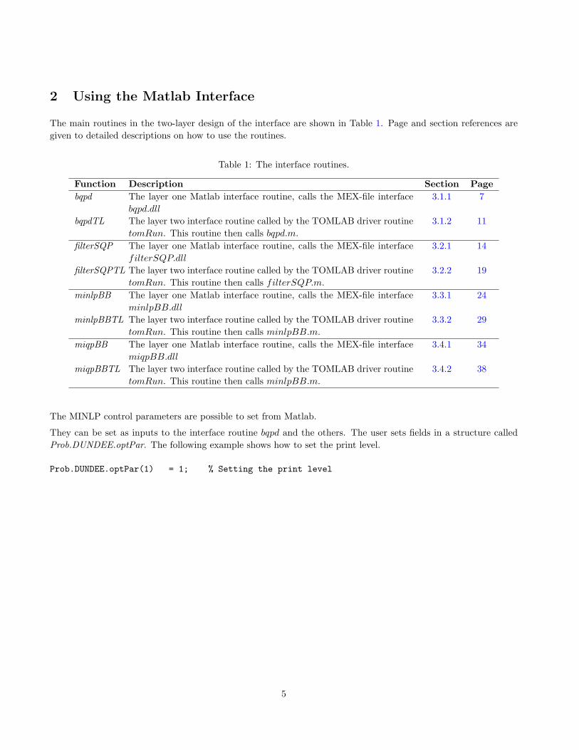
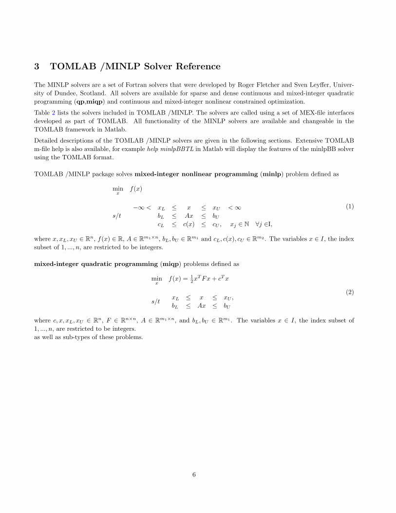
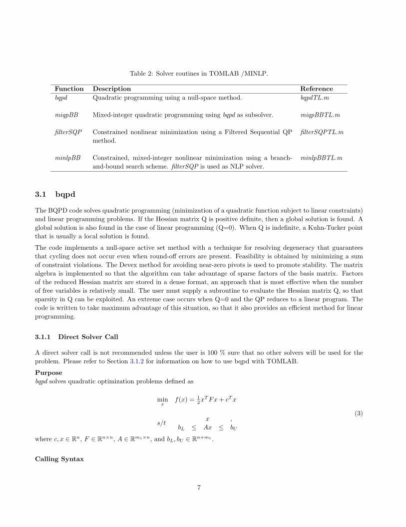
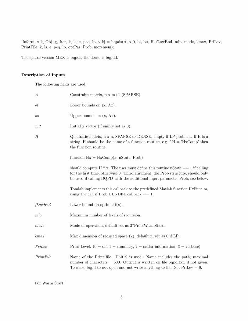
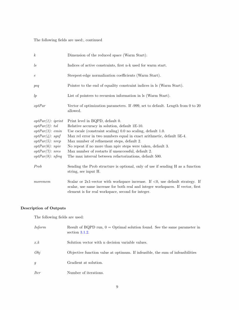

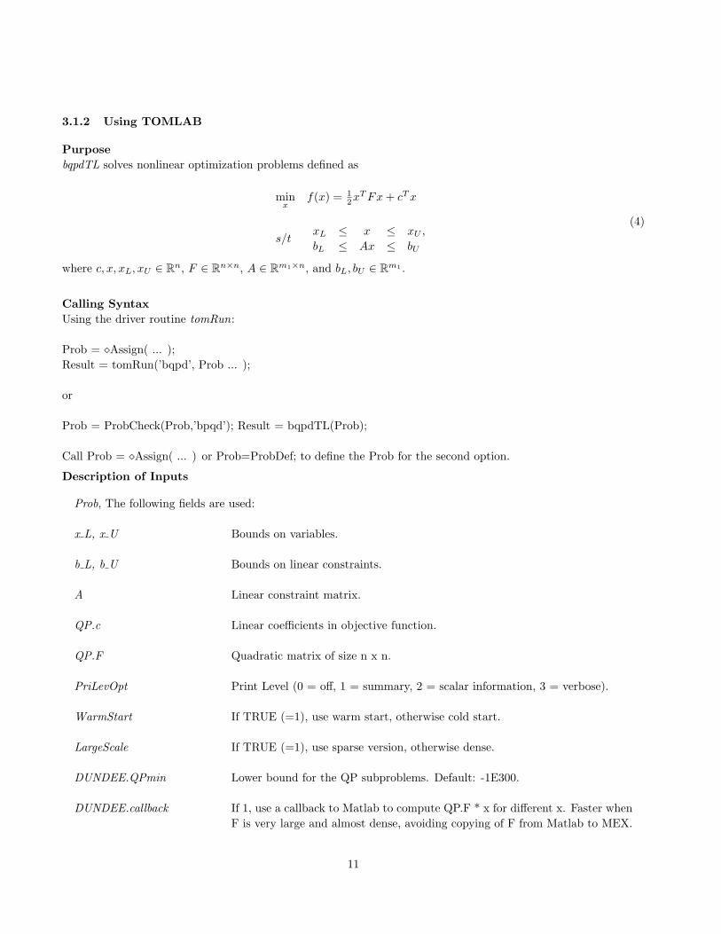
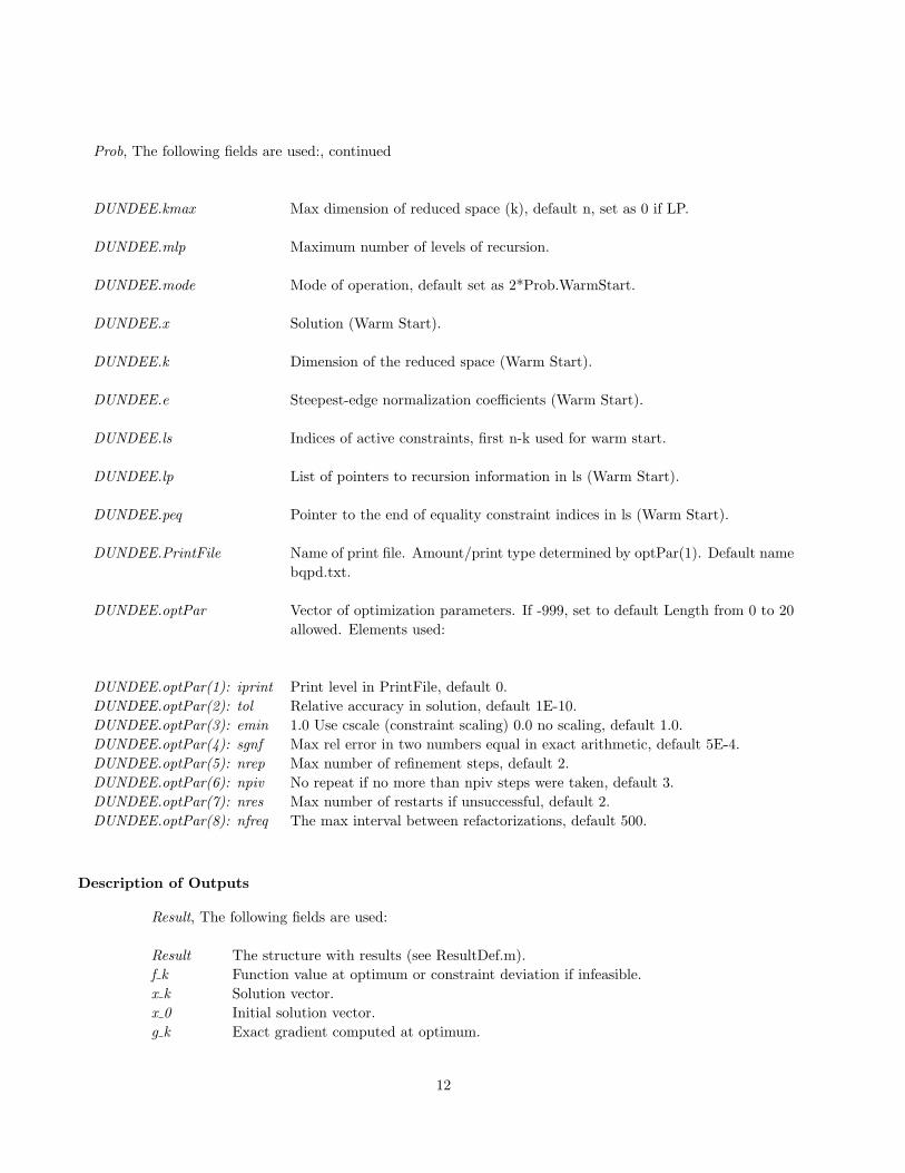
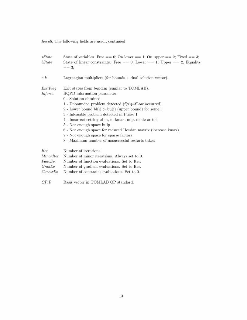
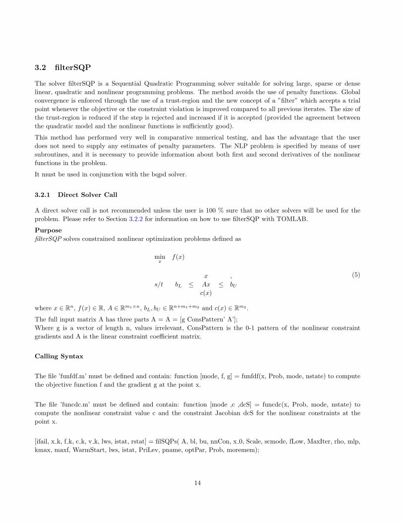
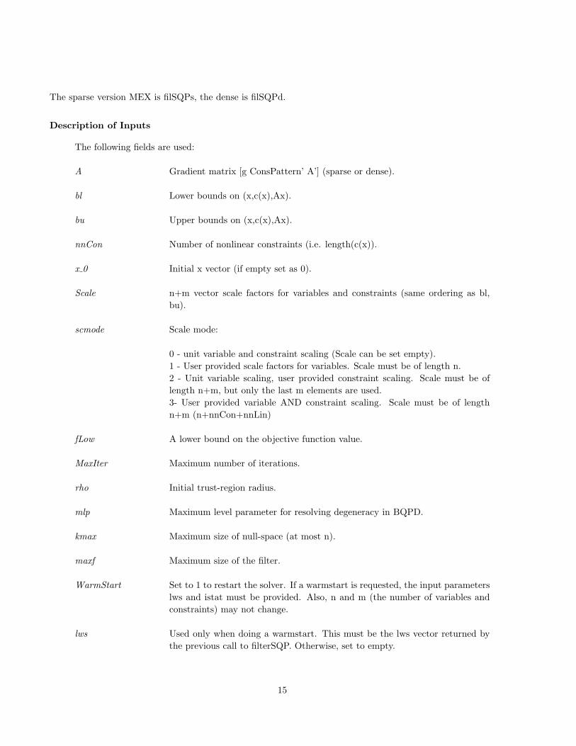
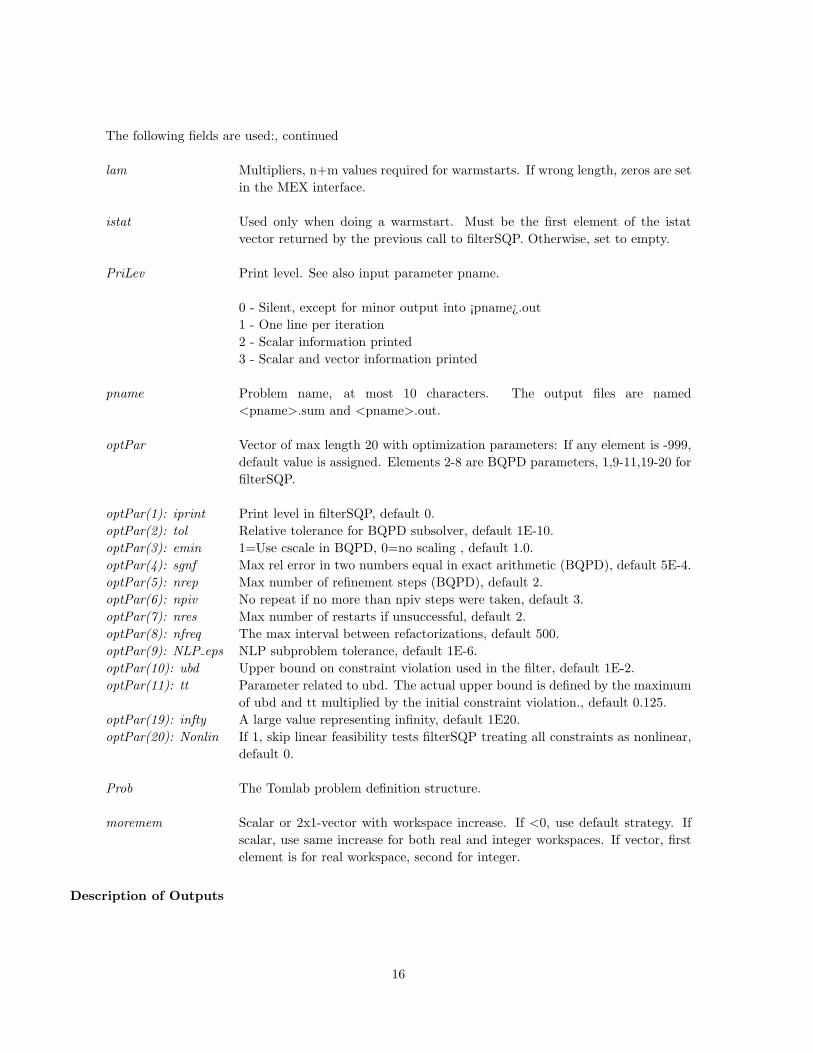
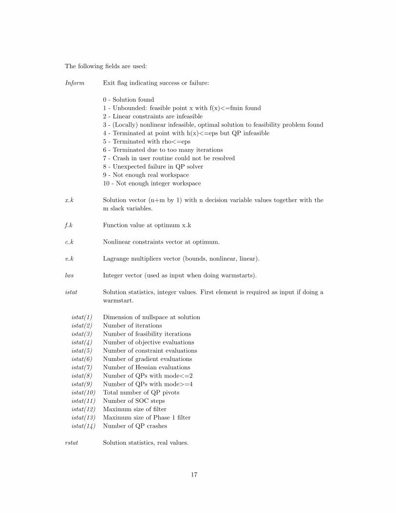

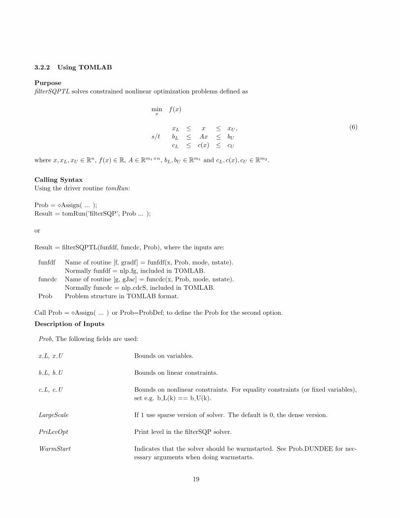
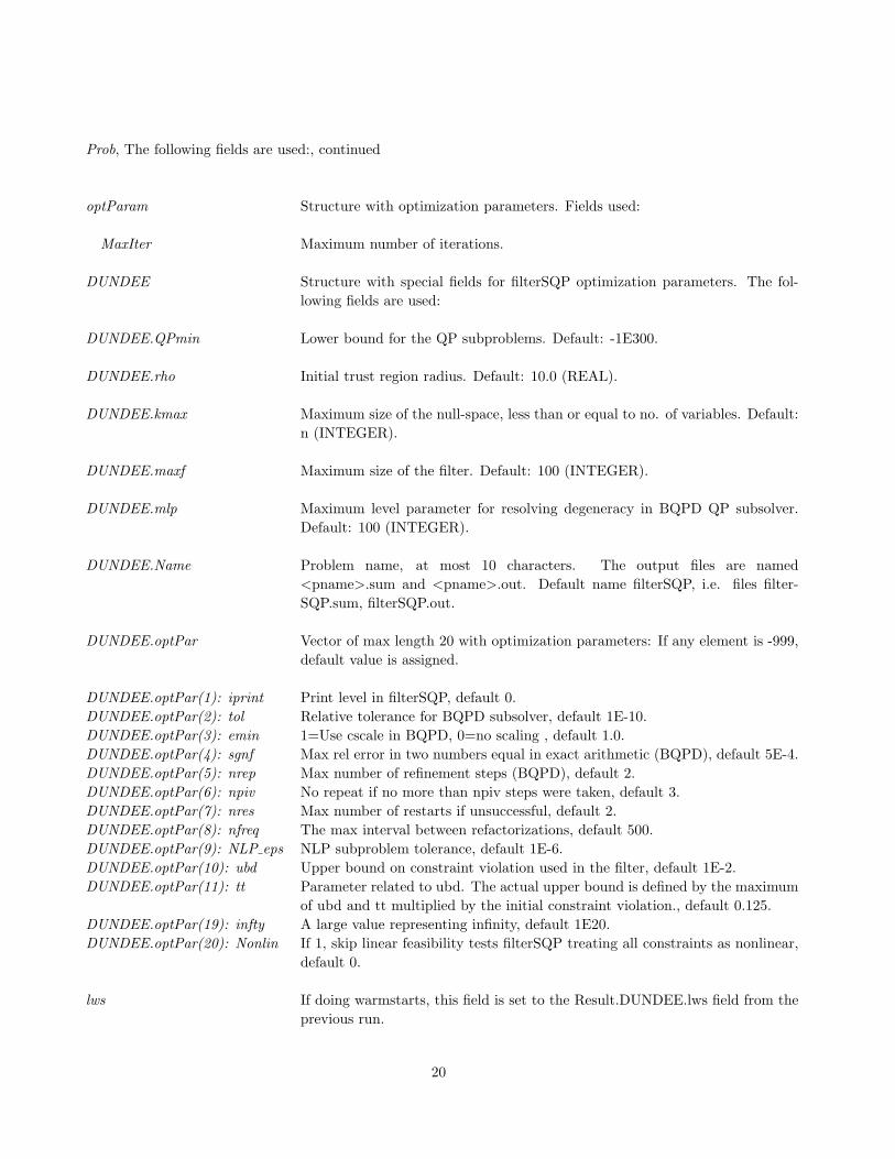
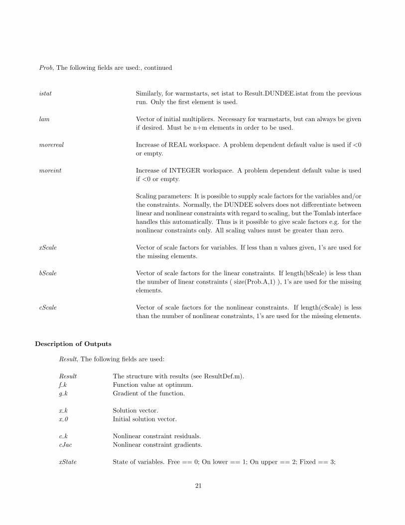
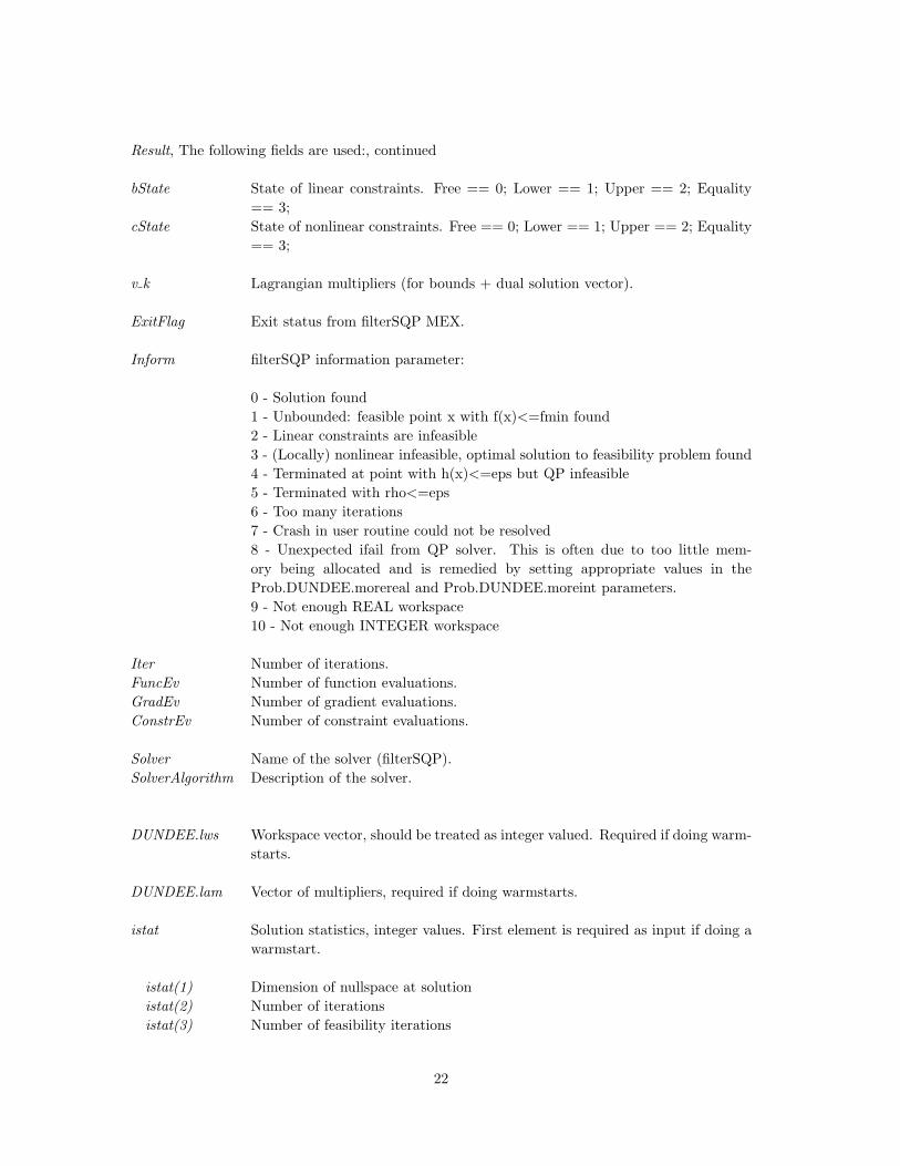
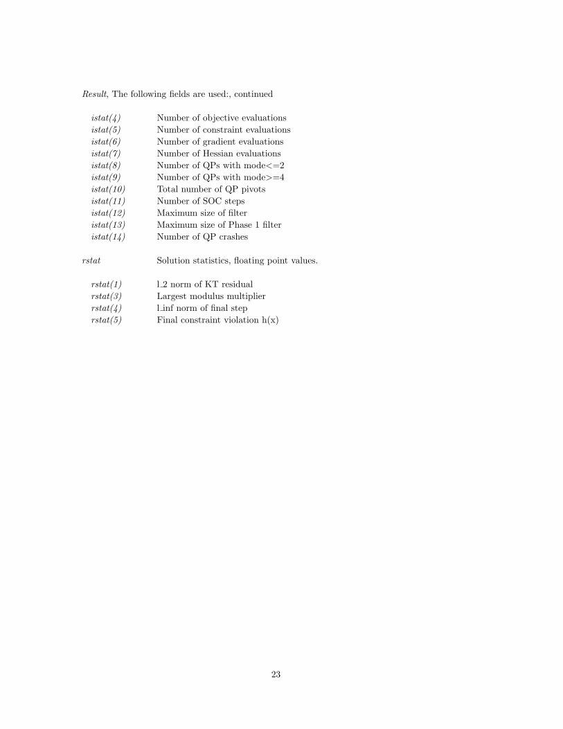

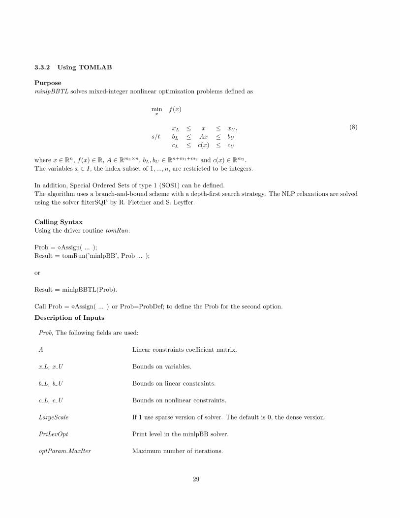
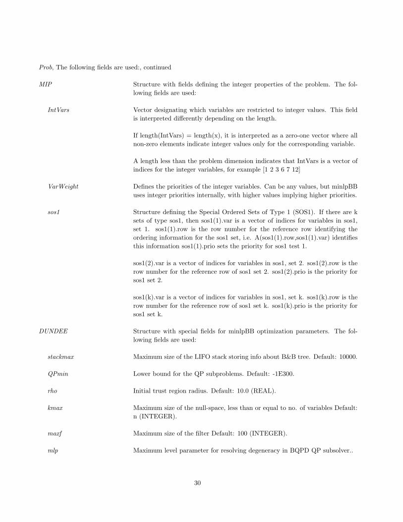
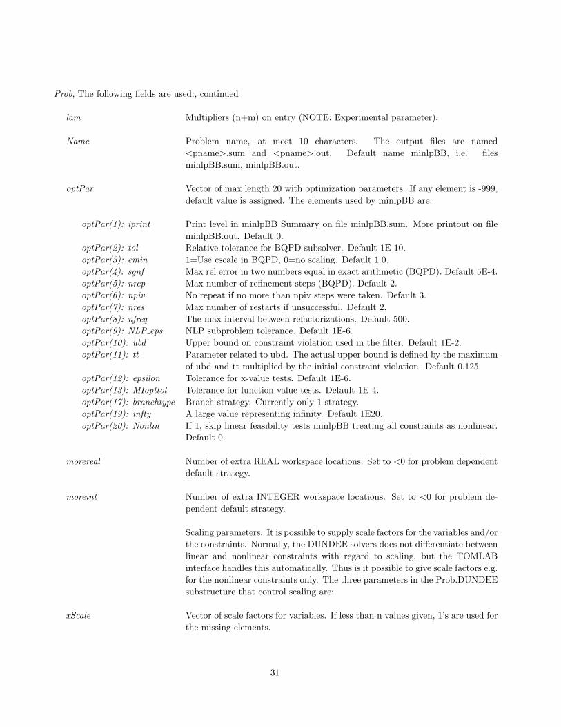
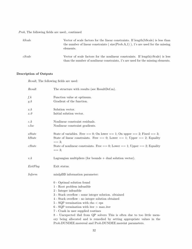
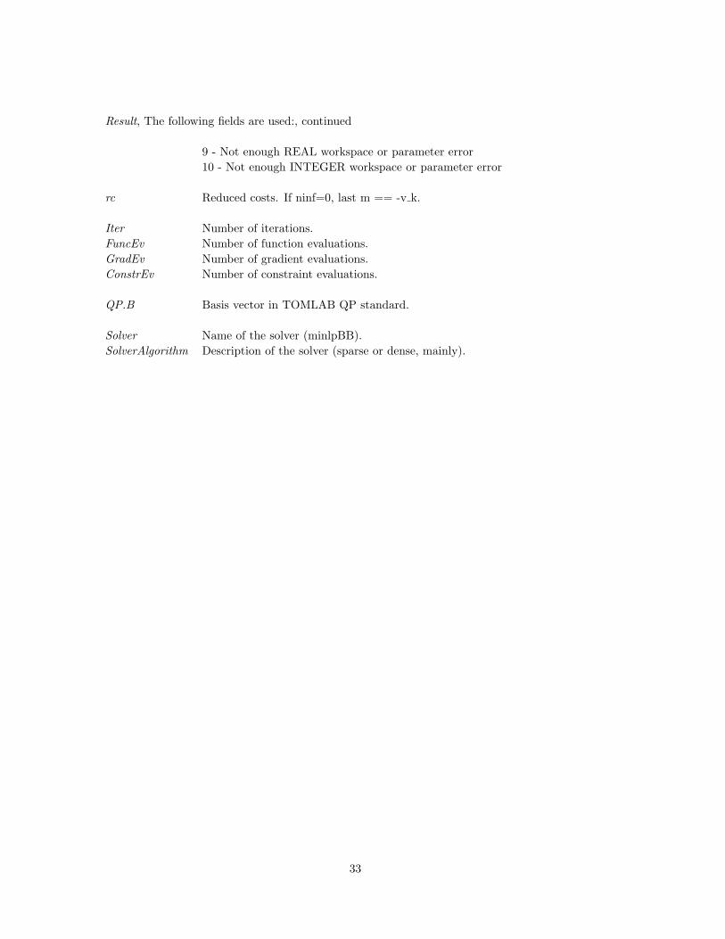
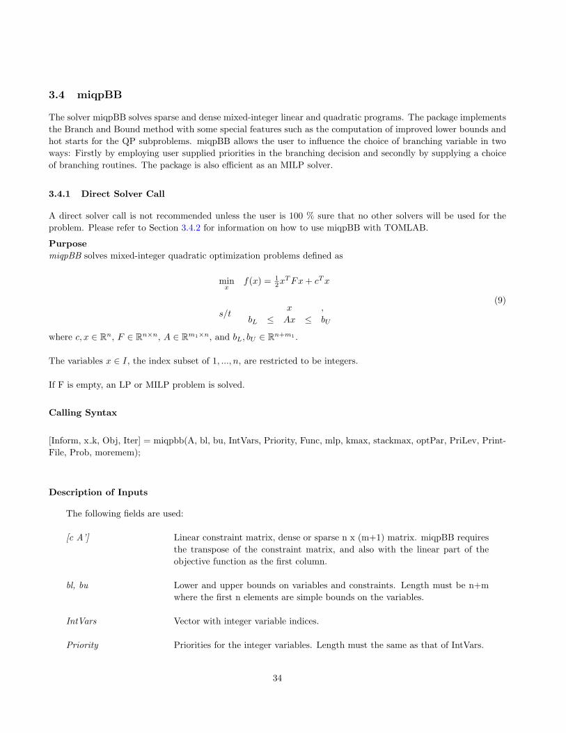
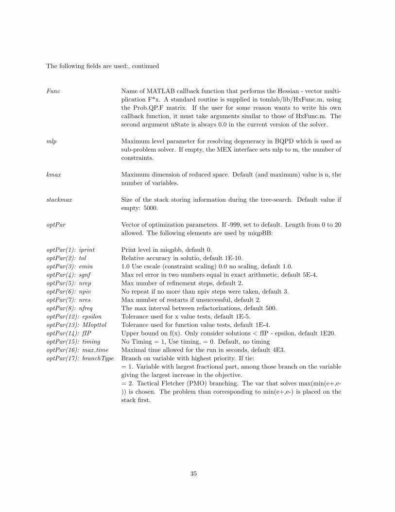
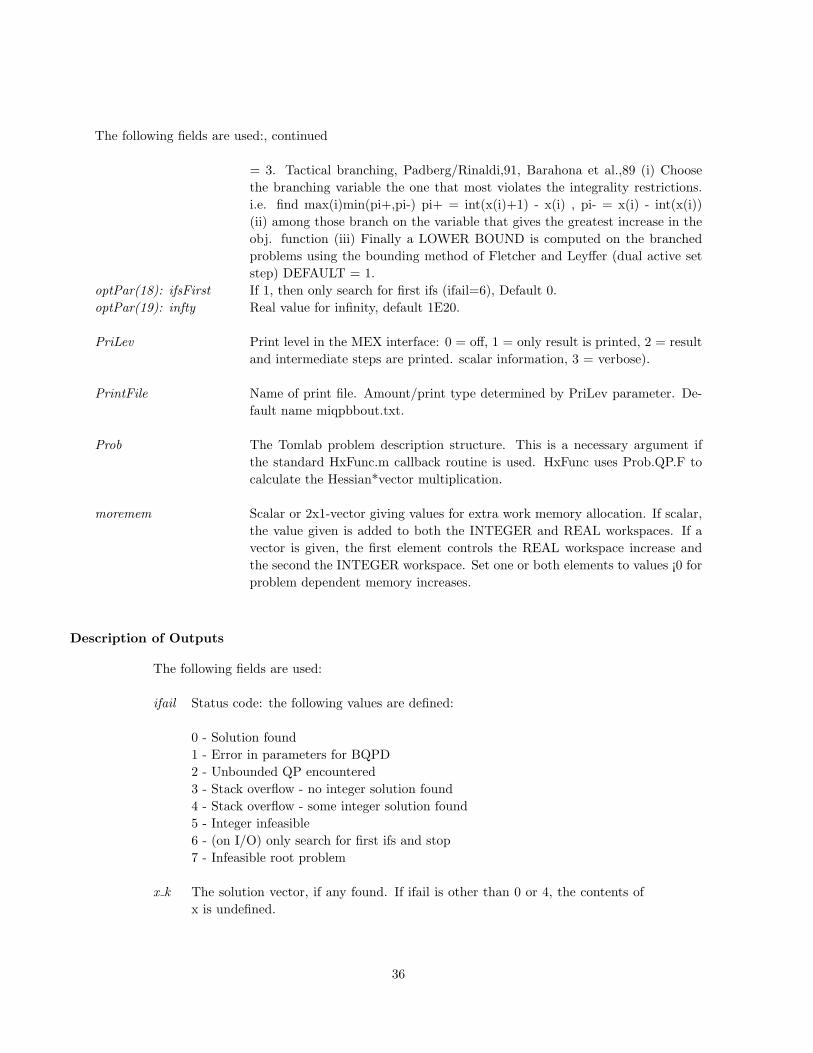

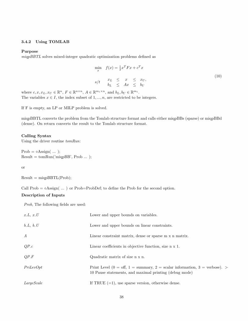
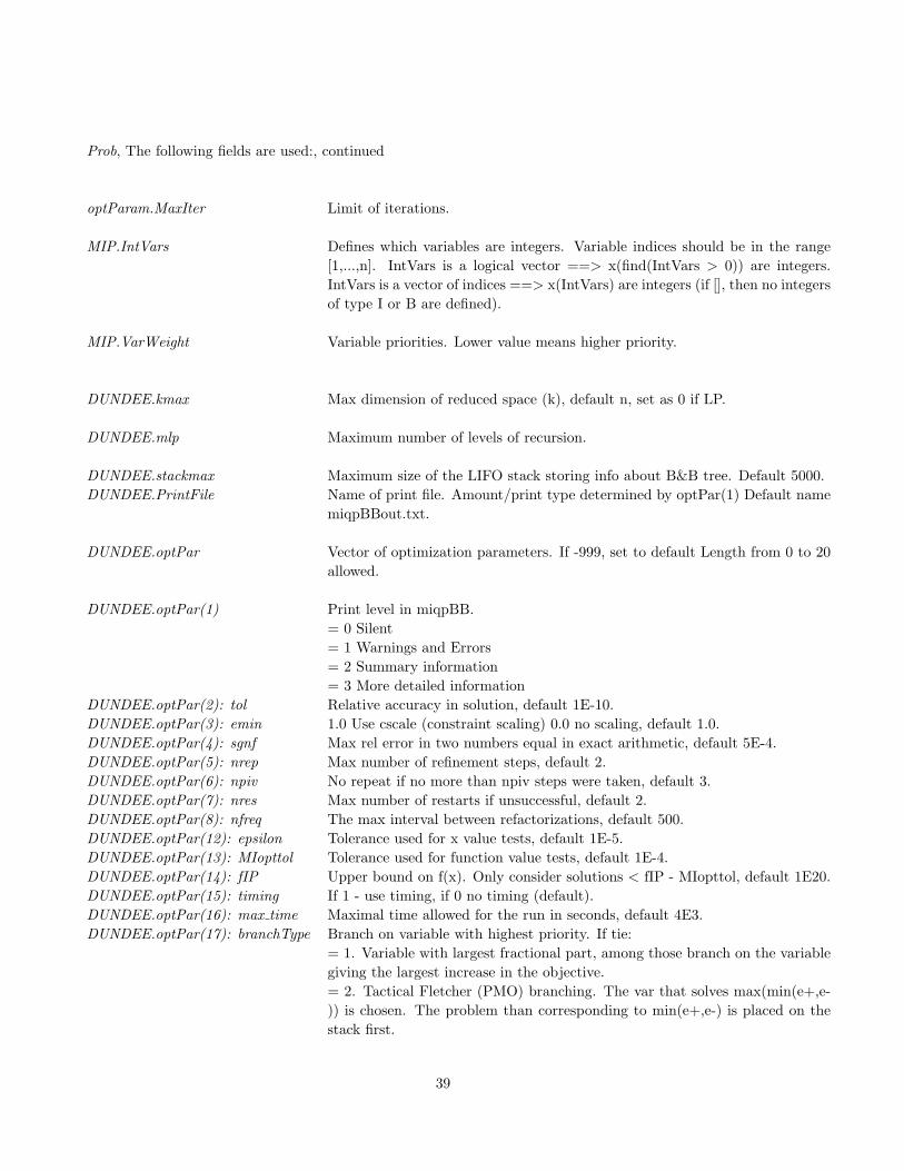
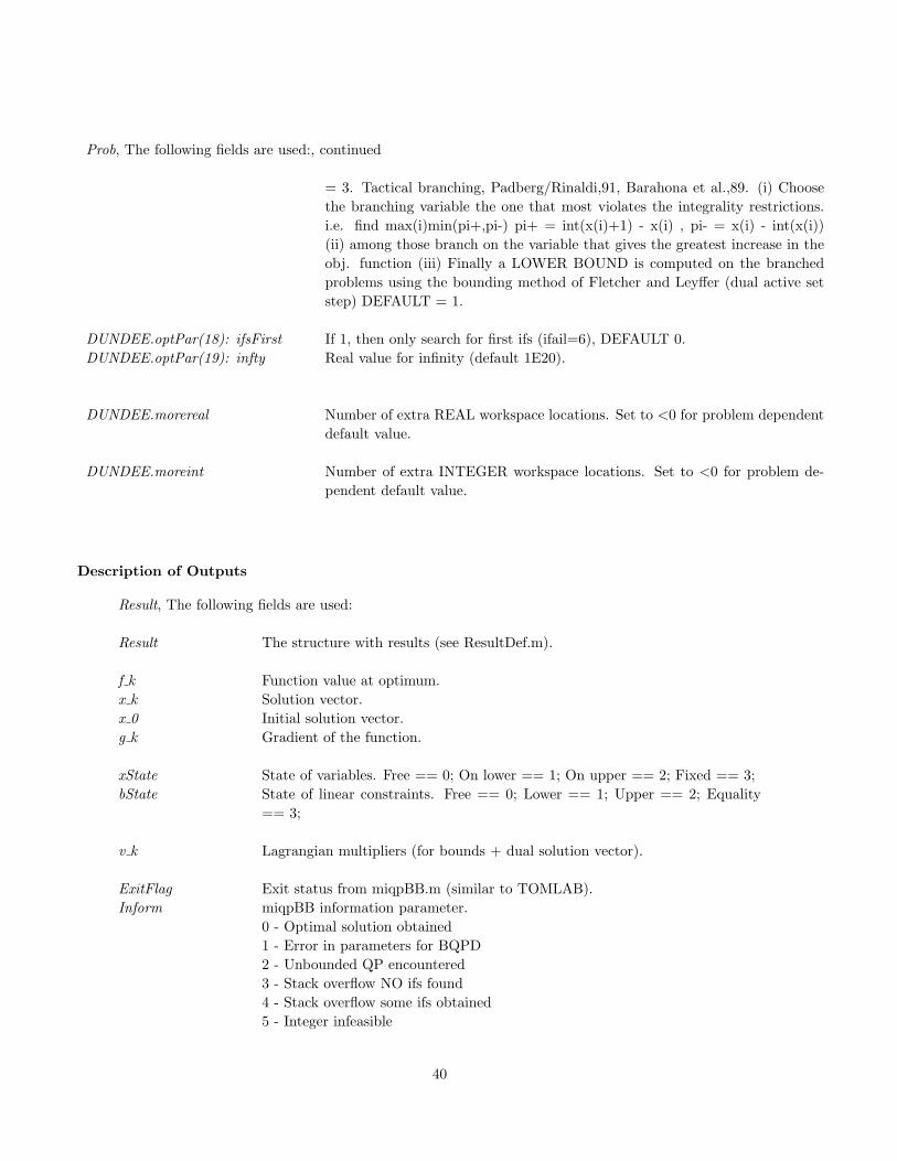
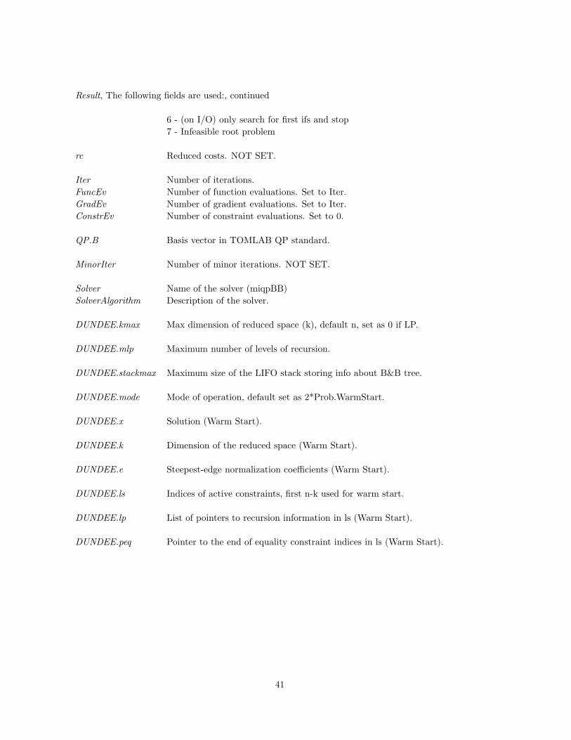
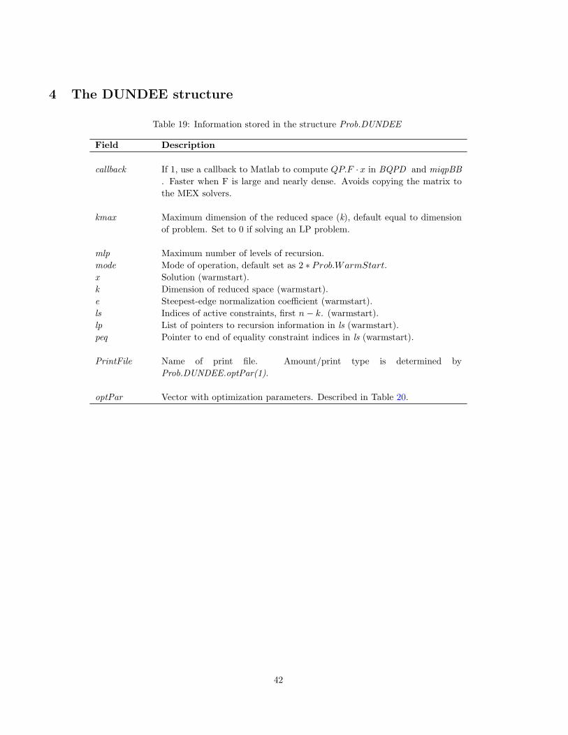
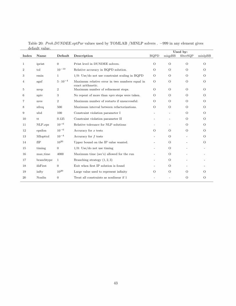
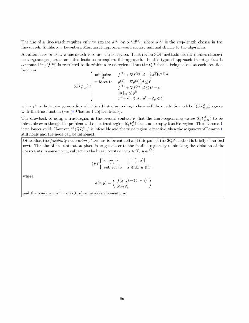
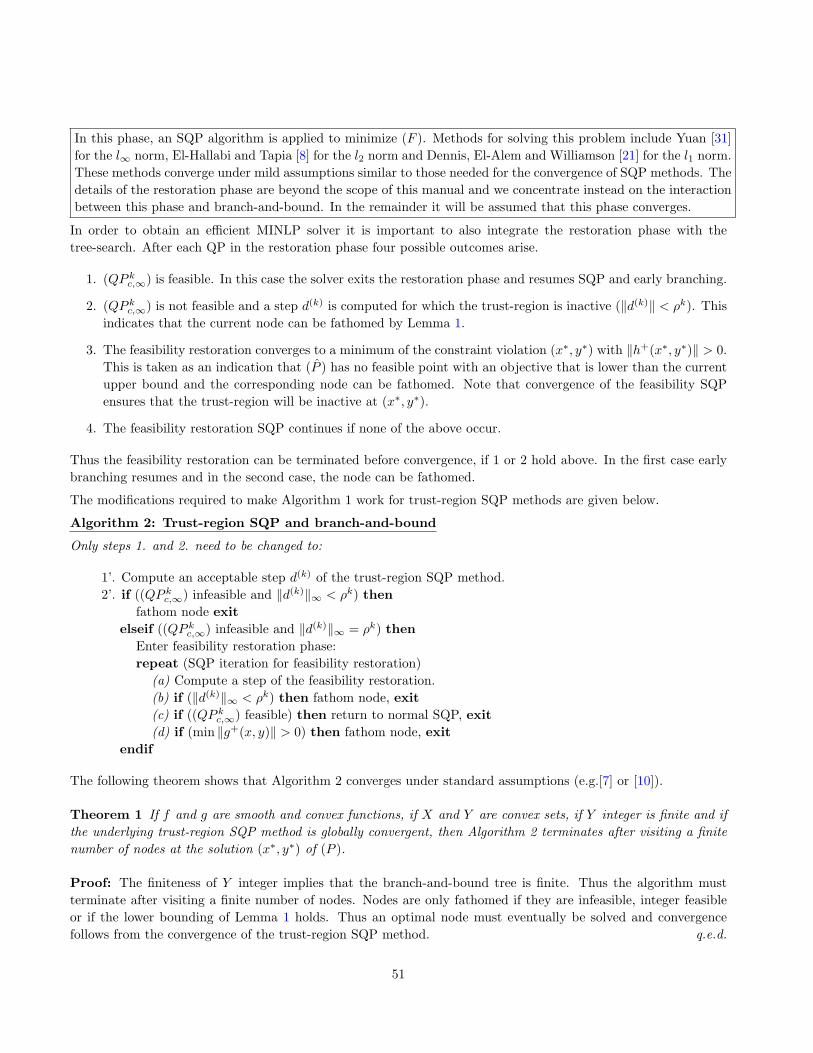
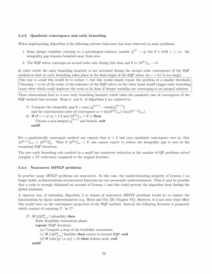
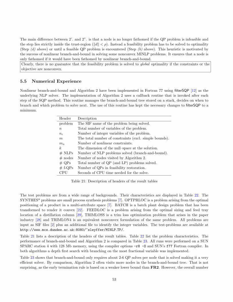
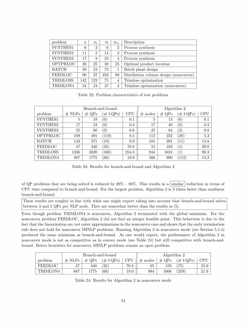

![Optimization for Machine Learning - Approximation Theory ... · [Austel et al., 2017] propose MINLP model Find simplest symbolic mathematical expression ... objective Constrain the](https://static.documents.pub/doc/80x56/5ccc9b9188c993b2538c9da1/optimization-for-machine-learning-approximation-theory-austel-et-al.jpg)


