USER’S GUIDE FOR TOMLAB 7 1 KennethHolmstr¨om 2 , Anders O. G¨ oran 3 and Marcus M. Edvall 4 May 5, 2010 -TOMLAB NOW INCLUDES THE MODELING ENGINE, TomSym [See section 4.3]! 1 More information available at the TOMLAB home page: http://tomopt.com/ and at the Applied Optimization and Modeling TOM home page http://www.ima.mdh.se/tom. E-mail: [email protected]. 2 Professor in Optimization, M¨alardalen University, Department of Mathematics and Physics, P.O. Box 883, SE-721 23 V¨aster˚ as, Sweden, [email protected]. 3 Tomlab Optimization AB, V¨aster˚ as Technology Park, Trefasgatan 4, SE-721 30 V¨aster˚ as, Sweden, [email protected]. 4 Tomlab Optimization Inc., 1260 SE Bishop Blvd Ste E, Pullman, WA 99163, USA, [email protected]. 1
Transcript
USER’S GUIDE FOR TOMLAB 71
Kenneth Holmstrom2, Anders O. Goran3 and Marcus M. Edvall4
May 5, 2010
-TOMLAB NOW INCLUDES THE MODELING ENGINE, TomSym [See section 4.3]!
1More information available at the TOMLAB home page: http://tomopt.com/ and at the Applied Optimization and Modeling
TOM home page http://www.ima.mdh.se/tom. E-mail: [email protected] in Optimization, Malardalen University, Department of Mathematics and Physics, P.O. Box 883, SE-721 23 Vasteras,
Sweden, [email protected] Optimization AB, Vasteras Technology Park, Trefasgatan 4, SE-721 30 Vasteras, Sweden, [email protected] Optimization Inc., 1260 SE Bishop Blvd Ste E, Pullman, WA 99163, USA, [email protected].
G Performance Tests on Linear Programming Solvers 258
References 264
7
1 Introduction
1.1 What is TOMLAB?
TOMLAB is a general purpose development, modeling and optimal control environment in Matlab for research,teaching and practical solution of optimization problems.
TOMLAB has grown out of the need for advanced, robust and reliable tools to be used in the development ofalgorithms and software for the solution of many different types of applied optimization problems.
There are many good tools available in the area of numerical analysis, operations research and optimization,but because of the different languages and systems, as well as a lack of standardization, it is a time consumingand complicated task to use these tools. Often one has to rewrite the problem formulation, rewrite the functionspecifications, or make some new interface routine to make everything work. Therefore the first obvious and basicdesign principle in TOMLAB is: Define your problem once, run all available solvers. The system takes care of allinterface problems, whether between languages or due to different demands on the problem specification.
In the process of optimization one sometimes wants to graphically view the problem and the solution process,especially for ill-conditioned nonlinear problems. Sometimes it is not clear what solver is best for the particulartype of problem and tests on different solvers can be of use. In teaching one wants to view the details of thealgorithms and look more carefully at the different algorithmic steps. When developing new algorithms tests onthousands of problems are necessary to fully access the pros and cons of the new algorithm. One might wantto solve a practical problem very many times, with slightly different conditions for the run. Or solve a controlproblem looping in real-time and solving the optimization problem each time slot.
All these issues and many more are addressed with the TOMLAB optimization environment. TOMLAB gives easyaccess to a large set of standard test problems, optimization solvers and utilities.
8
1.2 The Organization of This Guide
Section 2 presents the general design of TOMLAB.
Section 3 contains strict mathematical definitions of the optimization problem types. All solver routines availablein TOMLAB are described.
Section 4 describes the input format and modeling environment. The functionality of the modeling engineTomSym is discussed in 4.3 and also in appendix C.
Sections 5, 6, 7 and 8 contain examples on the process of defining problems and solving them. All test examplesare available as part of the TOMLAB distribution.
Section 9 shows how to setup and define multi layer optimization problems in TOMLAB.
Section 11 contains detailed descriptions of many of the functions in TOMLAB. The TOM solvers, originallydeveloped by the Applied Optimization and Modeling (TOM) group, are described together with TOMLAB driverroutine and utility functions. Other solvers, like the Stanford Optimization Laboratory (SOL) solvers are notdescribed, but documentation is available for each solver.
Section 12 describes the utility functions that can be used, for example tomRun and SolverList.
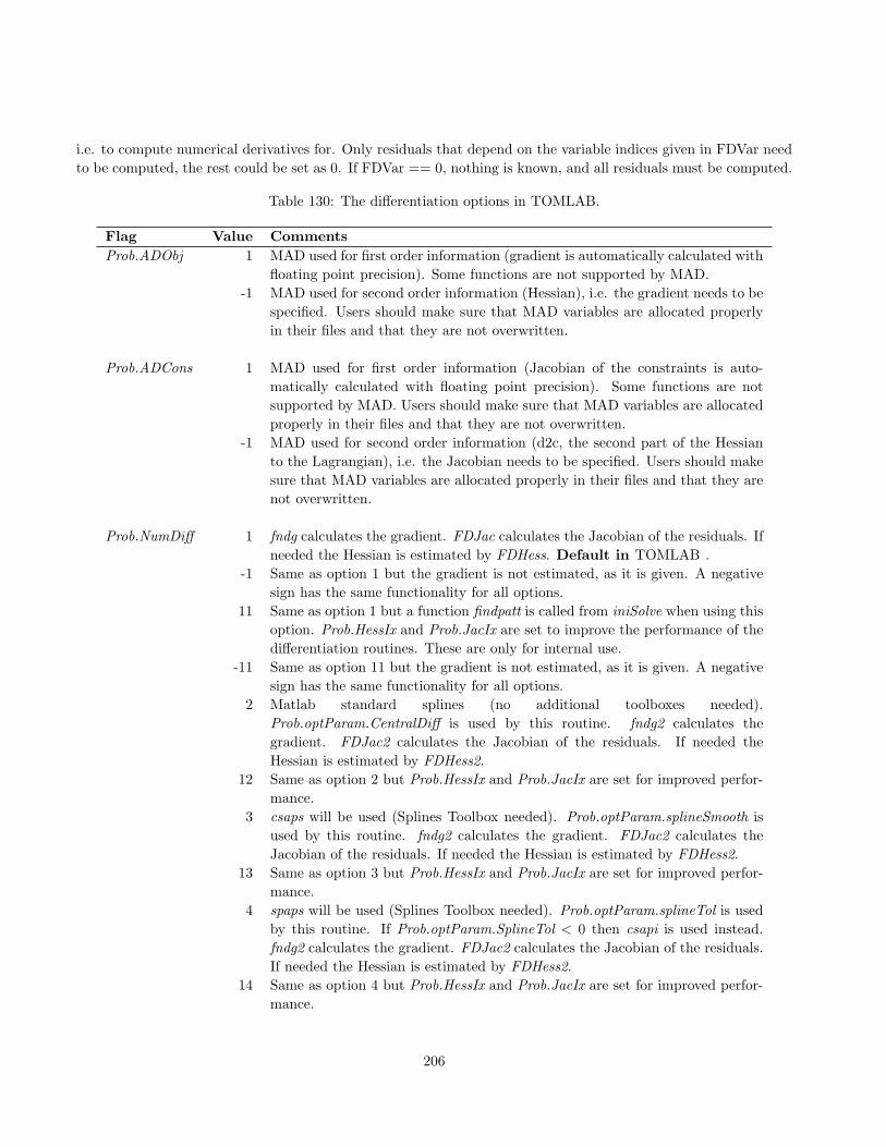
Section 13 introduces the different options for derivatives, automatic differentiation.
Section 14 discusses a number of special system features such as partially separable functions and user suppliedparameter information for the function computations.
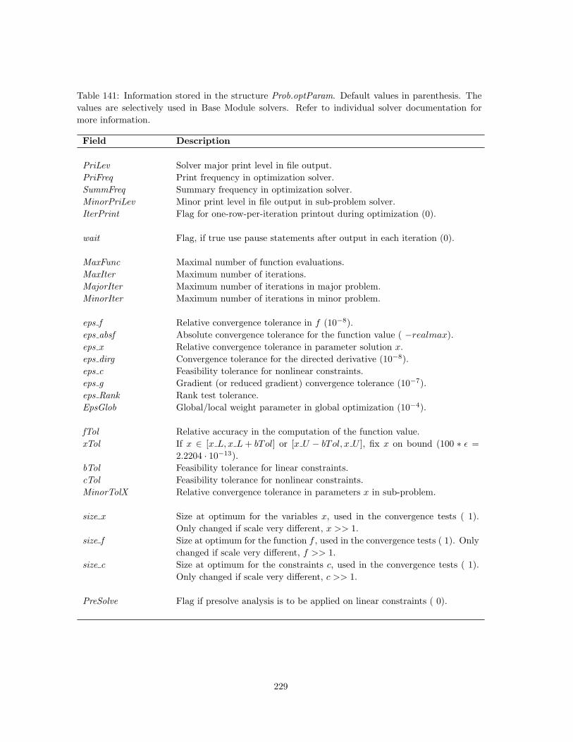
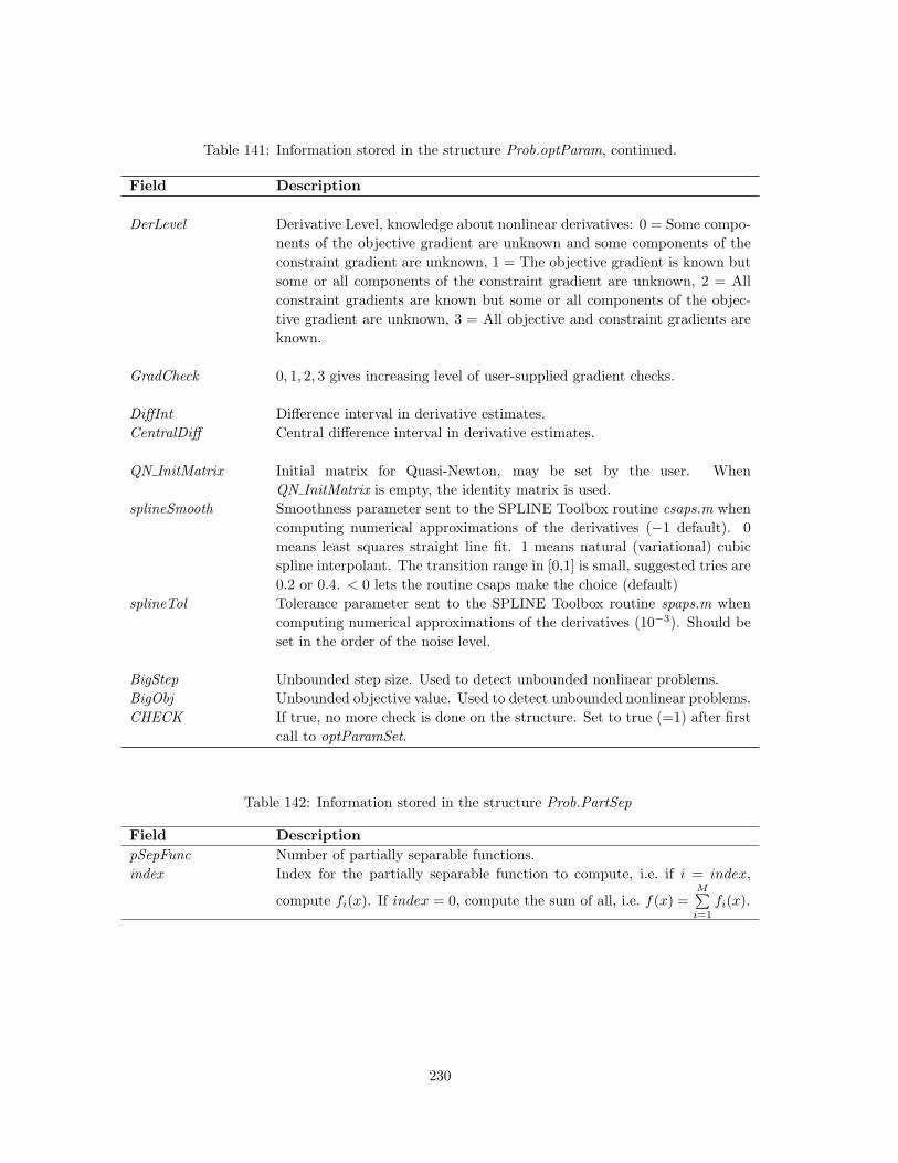
Appendix A contains tables describing all elements defined in the problem structure. Some subfields are eitherempty, or filled with information if the particular type of optimization problem is defined. To be able to setdifferent parameter options for the optimization solution, and change problem dependent information, the usershould consult the tables in this Appendix.
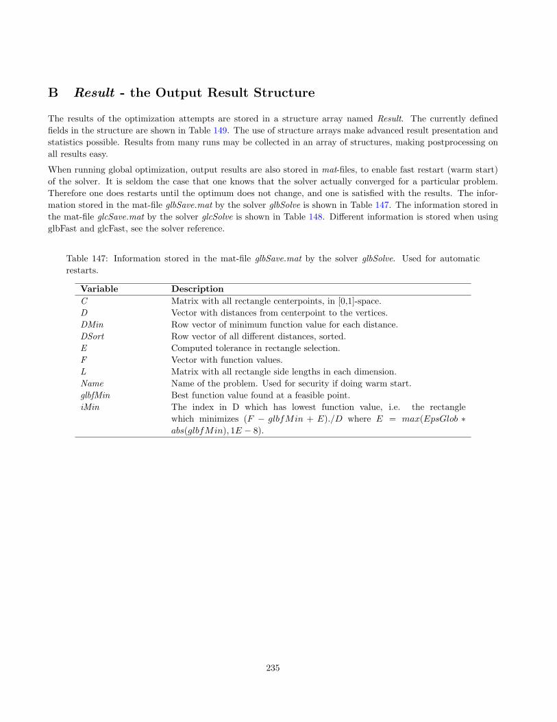
Appendix B contains tables describing all elements defined in the output result structure returned from all solversand driver routines.
Appendix D is concerned with the global variables used in TOMLAB and routines for handling important globalvariables enabling recursive calls of any depth.
Appendix E describes the available set of interfaces to other optimization software, such as CUTE, AMPL, andThe Mathworks’ Optimization Toolbox.
Appendix F gives some motivation for the development of TOMLAB.
9
1.3 Further Reading
TOMLAB has been discussed in several papers and at several conferences. The main paper on TOMLAB v1.0 is[42]. The use of TOMLAB for nonlinear programming and parameter estimation is presented in [45], and the useof linear and discrete optimization is discussed in [46]. Global optimization routines are also implemented, one isdescribed in [8].
In all these papers TOMLAB was divided into two toolboxes, the NLPLIB TB and the OPERA TB. TOMLAB v2.0was discussed in [43], [40]. and [41]. TOMLAB v4.0 and how to solve practical optimization problems withTOMLAB is discussed in [44].
The use of TOMLAB for costly global optimization with industrial applications is discussed in [9]; costly globaloptimization with financial applications in [37, 38, 39]. Applications of global optimization for robust control ispresented in [25, 26]. The use of TOMLAB for exponential fitting and nonlinear parameter estimation are discussedin e.g. [49, 4, 22, 23, 47, 48].
The manuals for the add-on solver packages are also recommended reading material.
10
2 Overall Design
The scope of TOMLAB is large and broad, and therefore there is a need of a well-designed system. It is alsonatural to use the power of the Matlab language, to make the system flexible and easy to use and maintain. Theconcept of structure arrays is used and the ability in Matlab to execute Matlab code defined as string expressionsand to execute functions specified by a string.
2.1 Structure Input and Output
Normally, when solving an optimization problem, a direct call to a solver is made with a long list of parametersin the call. The parameter list is solver-dependent and makes it difficult to make additions and changes to thesystem.
TOMLAB solves the problem in two steps. First the problem is defined and stored in a Matlab structure. Then thesolver is called with a single argument, the problem structure. Solvers that were not originally developed for theTOMLAB environment needs the usual long list of parameters. This is handled by the driver routine tomRun.mwhich can call any available solver, hiding the details of the call from the user. The solver output is collected in astandardized result structure and returned to the user.
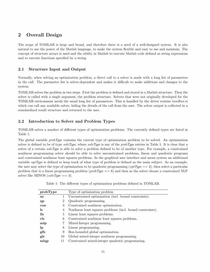
2.2 Introduction to Solver and Problem Types
TOMLAB solves a number of different types of optimization problems. The currently defined types are listed inTable 1.
The global variable probType contains the current type of optimization problem to be solved. An optimizationsolver is defined to be of type solvType, where solvType is any of the probType entries in Table 1. It is clear that asolver of a certain solvType is able to solve a problem defined to be of another type. For example, a constrainednonlinear programming solver should be able to solve unconstrained problems, linear and quadratic programsand constrained nonlinear least squares problems. In the graphical user interface and menu system an additionalvariable optType is defined to keep track of what type of problem is defined as the main subject. As an example,the user may select the type of optimization to be quadratic programming (optType == 2), then select a particularproblem that is a linear programming problem (probType == 8) and then as the solver choose a constrained NLPsolver like MINOS (solvType == 3).
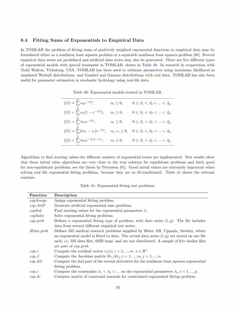
Table 1: The different types of optimization problems defined in TOMLAB.
probType Type of optimization problemuc 1 Unconstrained optimization (incl. bound constraints).qp 2 Quadratic programming.con 3 Constrained nonlinear optimization.ls 4 Nonlinear least squares problems (incl. bound constraints).lls 5 Linear least squares problems.cls 6 Constrained nonlinear least squares problems.mip 7 Mixed-Integer programming.lp 8 Linear programming.glb 9 Box-bounded global optimization.glc 10 Global mixed-integer nonlinear programming.miqp 11 Constrained mixed-integer quadratic programming.
11
Table 1: The different types of optimization problems defined in TOMLAB, continued
probType Type of optimization problemminlp 12 Constrained mixed-integer nonlinear optimization.lmi 13 Semi-definite programming with Linear Matrix Inequalities.bmi 14 Semi-definite programming with Bilinear Matrix Inequalities.exp 15 Exponential fitting problems.nts 16 Nonlinear Time Series.lcp 22 Linear Mixed-Complimentary Problems.mcp 23 Nonlinear Mixed-Complimentary Problems.
Please note that since the actual numbers used for probType may change in future releases, it is recommended touse the text abbreviations. See help for checkType for further information.
Define probSet to be a set of defined optimization problems belonging to a certain class of problems of typeprobType. Each probSet is physically stored in one file, an Init File. In Table 2 the currently defined problem setsare listed, and new probSet sets are easily added.
Table 2: Defined test problem sets in TOMLAB. probSets marked with ∗ are not part of thestandard distribution
probSet probType Description of test problem setuc 1 Unconstrained test problems.qp 2 Quadratic programming test problems.con 3 Constrained test problems.ls 4 Nonlinear least squares test problems.lls 5 Linear least squares problems.cls 6 Linear constrained nonlinear least squares problems.mip 7 Mixed-integer programming problems.lp 8 Linear programming problems.glb 9 Box-bounded global optimization test problems.glc 10 Global MINLP test problems.
lmi 13 Semi-definite programming with Linear Matrix Inequalities.bmi 14 Semi-definite programming with Bilinear Matrix Inequalities.exp 15 Exponential fitting problems.nts 16 Nonlinear time series problems.lcp 22 Linear mixed-complimentary problems.
mcp 23 Nonlinear mixed-complimentary problems.
mgh 4 More, Garbow, Hillstrom nonlinear least squares problems.chs 3 Hock-Schittkowski constrained test problems.uhs 1 Hock-Schittkowski unconstrained test problems.
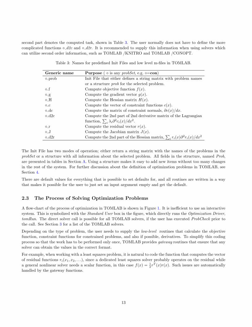
The names of the predefined Init Files that do the problem setup, and the corresponding low level routines areconstructed as two parts. The first part being the abbreviation of the relevant probSet, see Table 2, and the
12
second part denotes the computed task, shown in Table 3. The user normally does not have to define the morecomplicated functions � d2c and � d2r. It is recommended to supply this information when using solvers whichcan utilize second order information, such as TOMLAB /KNITRO and TOMLAB /CONOPT.
Table 3: Names for predefined Init Files and low level m-files in TOMLAB.
Generic name Purpose ( � is any probSet, e.g. �=con)� prob Init File that either defines a string matrix with problem names
or a structure prob for the selected problem.� f Compute objective function f(x).� g Compute the gradient vector g(x).� H Compute the Hessian matrix H(x).� c Compute the vector of constraint functions c(x).� dc Compute the matrix of constraint normals, ∂c(x)/dx.� d2c Compute the 2nd part of 2nd derivative matrix of the Lagrangian
function,∑i λi∂
2ci(x)/dx2.� r Compute the residual vector r(x).� J Compute the Jacobian matrix J(x).� d2r Compute the 2nd part of the Hessian matrix,
∑i ri(x)∂2ri(x)/dx2
The Init File has two modes of operation; either return a string matrix with the names of the problems in theprobSet or a structure with all information about the selected problem. All fields in the structure, named Prob,are presented in tables in Section A. Using a structure makes it easy to add new items without too many changesin the rest of the system. For further discussion about the definition of optimization problems in TOMLAB, seeSection 4.
There are default values for everything that is possible to set defaults for, and all routines are written in a waythat makes it possible for the user to just set an input argument empty and get the default.
2.3 The Process of Solving Optimization Problems
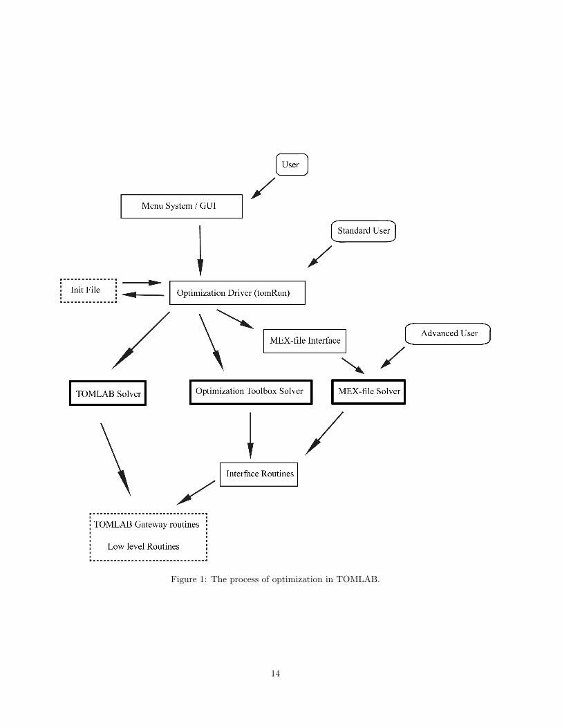
A flow-chart of the process of optimization in TOMLAB is shown in Figure 1. It is inefficient to use an interactivesystem. This is symbolized with the Standard User box in the figure, which directly runs the Optimization Driver,tomRun. The direct solver call is possible for all TOMLAB solvers, if the user has executed ProbCheck prior tothe call. See Section 3 for a list of the TOMLAB solvers.
Depending on the type of problem, the user needs to supply the low-level routines that calculate the objectivefunction, constraint functions for constrained problems, and also if possible, derivatives. To simplify this codingprocess so that the work has to be performed only once, TOMLAB provides gateway routines that ensure that anysolver can obtain the values in the correct format.
For example, when working with a least squares problem, it is natural to code the function that computes the vectorof residual functions ri(x1, x2, . . .), since a dedicated least squares solver probably operates on the residual whilea general nonlinear solver needs a scalar function, in this case f(x) = 1
2rT (x)r(x). Such issues are automatically
handled by the gateway functions.
13
Figure 1: The process of optimization in TOMLAB.
14
2.4 Low Level Routines and Gateway Routines
Low level routines are the routines that compute:
• The objective function value
• The gradient vector
• The Hessian matrix (second derivative matrix)
• The residual vector (for nonlinear least squares problems)
• The Jacobian matrix (for nonlinear least squares problems)
• The vector of constraint functions
• The matrix of constraint normals (the constraint Jacobian)
• The second part of the second derivative of the Lagrangian function.
The last three routines are only needed for constrained problems.
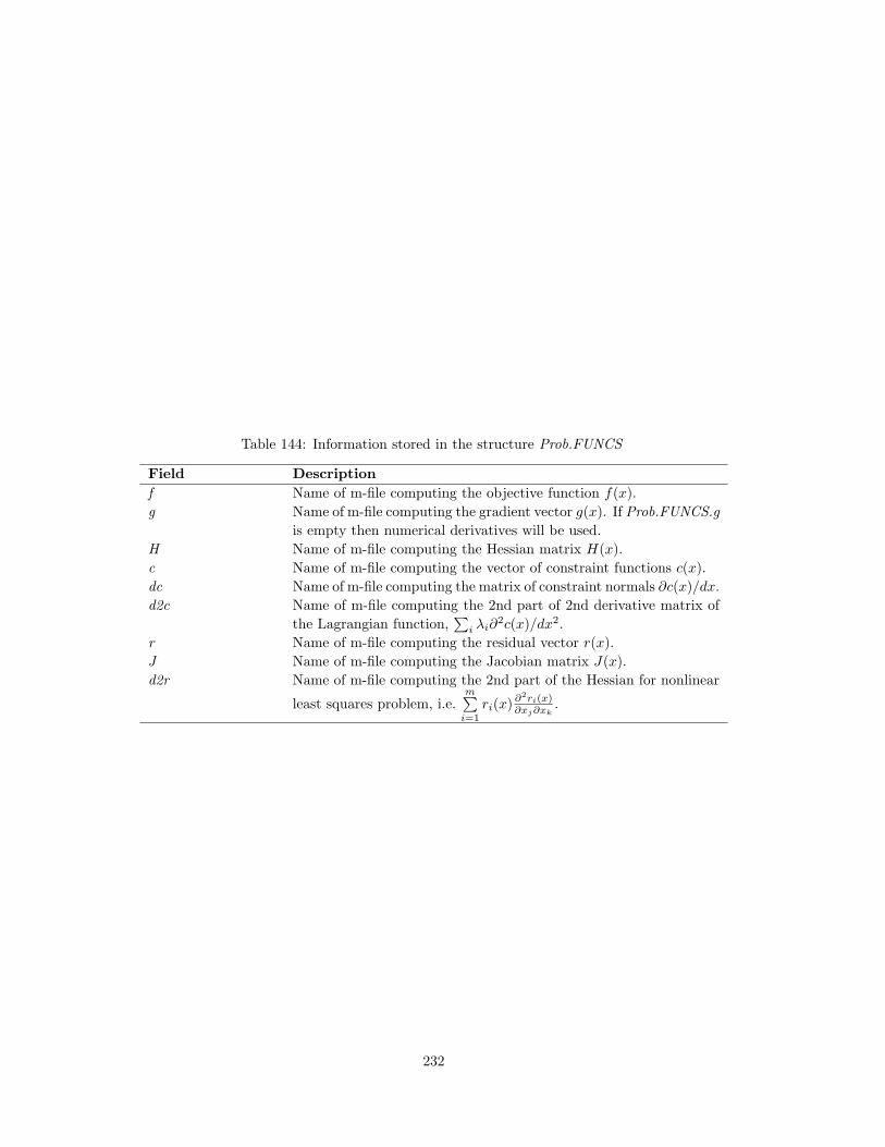
The names of these routines are defined in the structure fields Prob.FUNCS.f, Prob.FUNCS.g, Prob.FUNCS.H etc.It is the task for the Assign routine to set the names of the low level m-files. This is done by a call to the routineconAssign with the names as arguments for example. There are Assign routines for all problem types handled byTOMLAB. As an example, see ’help conAssign’ in MATLAB.
pSepFunc, fLowBnd, A, b_L, b_U, ’c’, ’dc’, ’d2c’, ConsPattern,...
c_L, c_U, x_min, x_max, f_opt, x_opt);
Only the low level routines relevant for a certain type of optimization problem need to be coded. There are dummyroutines for the others. Numerical differentiation is automatically used for gradient, Jacobian and constraintgradient if the corresponding user routine is non present or left out when calling conAssign. However, the solveralways needs more time to estimate the derivatives compared to if the user supplies a code for them. Also thenumerical accuracy is lower for estimated derivatives, so it is recommended that the user always tries to code thederivatives, if it is possible. Another option is automatic differentiation with TOMLAB /MAD.
TOMLAB uses gateway routines (nlp f, nlp g, nlp H, nlp c, nlp dc, nlp d2c, nlp r, nlp J, nlp d2r). These routinesextract the search directions and line search steps, count iterations, handle separable functions, keep track of thekind of differentiation wanted etc. They also handle the separable NLLS case and NLLS weighting. By the use ofglobal variables, unnecessary evaluations of the user supplied routines are avoided.
To get a picture of how the low-level routines are used in the system, consider Figure 2 and 3. Figure 2 illustratesthe chain of calls when computing the objective function value in ucSolve for a nonlinear least squares problemdefined in mgh prob, mgh r and mgh J. Figure 3 illustrates the chain of calls when computing the numericalapproximation of the gradient (by use of the routine fdng) in ucSolve for an unconstrained problem defined inuc prob and uc f.
Information about a problem is stored in the structure variable Prob, described in detail in the tables in AppendixA. This variable is an argument to all low level routines. In the field element Prob.user, problem specific information
Figure 2: The chain of calls when computing the objective function value in ucSolve for a nonlinear leastsquares problem defined in mgh prob, mgh r and mgh J.
ucSolve <==> nlp_g <==> fdng <==> nlp_r <==> uc_f
Figure 3: The chain of calls when computing the numerical approximation of the gradient in ucSolve foran unconstrained problem defined in uc prob and uc f.
needed to evaluate the low level routines are stored. This field is most often used if problem related questionsare asked when generating the problem. It is often the case that the user wants to supply the low-level routineswith additional information besides the variables x that are optimized. Any unused fields could be defined in thestructure Prob for that purpose. To avoid potential conflicts with future TOMLAB releases, it is recommendedto use subfields of Prob.user. It the user wants to send some variables a, B and C, then, after creating the Probstructure, these extra variables are added to the structure:
Prob.user.a=a;
Prob.user.B=B;
Prob.user.C=C;
Then, because the Prob structure is sent to all low-level routines, in any of these routines the variables are pickedout from the structure:
a = Prob.user.a;
B = Prob.user.B;
C = Prob.user.C;
A more detailed description of how to define new problems is given in sections 5, 6 and 8. The usage of Prob.useris described in Section 14.2.
Different solvers all have different demand on how information should be supplied, i.e. the function to optimize, thegradient vector, the Hessian matrix etc. To be able to code the problem only once, and then use this formulationto run all types of solvers, interface routines that returns information in the format needed for the relevant solverwere developed.
Table 4 describes the low level test functions and the corresponding Init File routine needed for the predefinedconstrained optimization (con) problems. For the predefined unconstrained optimization (uc) problems, theglobal optimization (glb, glc) problems and the quadratic programming problems (qp) similar routines have beendefined.
To conclude, the system design is flexible and easy to expand in many different ways.
16
Table 4: Generally constrained nonlinear (con) test problems.
Function Descriptioncon prob Init File. Does the initialization of the con test problems.con f Compute the objective function f(x) for con test problems.con g Compute the gradient g(x) for con test problems. xcon H Compute the Hessian matrix H(x) of f(x) for con test problems.con c Compute the constraint residuals c(x) for con test problems.con dc Compute the derivative of the constraint residuals for con test problems.con d2c Compute the 2nd part of 2nd derivative matrix of the Lagrangian function,∑
i λi∂2ci(x)/dx2 for con test problems.
con fm Compute merit function θ(xk).con gm Compute gradient of merit function θ(xk).
17
3 Problem Types and Solver Routines
Section 3.1 defines all problem types in TOMLAB. Each problem definition is accompanied by brief suggestionson suitable solvers. This is followed in Section 3.2 by a complete list of the available solver routines in TOMLABand the various available extensions, such as /SOL and /CGO.
3.1 Problem Types Defined in TOMLAB
The unconstrained optimization (uc) problem is defined as
minx
f(x)
s/t xL ≤ x ≤ xU ,
(1)
where x, xL, xU ∈ Rn and f(x) ∈ R. For unbounded variables, the corresponding elements of xL, xU may be setto ±∞.
Recommended solvers: TOMLAB /KNITRO and TOMLAB /SNOPT.
The TOMLAB Base Module routine ucSolve includes several of the most popular search step methods for uncon-strained optimization. Bound constraints are treated as described in Gill et. al. [28]. The search step methodsfor unconstrained optimization included in ucSolve are: the Newton method, the quasi-Newton BFGS and DFPmethod, the Fletcher-Reeves and Polak-Ribiere conjugate-gradient method, and the Fletcher conjugate descentmethod. The quasi-Newton methods may either update the inverse Hessian (standard) or the Hessian itself. TheNewton method and the quasi-Newton methods updating the Hessian use a subspace minimization technique tohandle rank problems, see Lindstrom [53]. The quasi-Newton algorithms also use safe guarding techniques to avoidrank problem in the updated matrix.
Another TOMLAB Base Module solver suitable for unconstrained problems is the structural trust region algorithmsTrustr, combined with an initial trust region radius algorithm. The code is based on the algorithms in [13] and[67], and treats partially separable functions. Safeguarded BFGS or DFP are used for the quasi-Newton update,if the analytical Hessian is not used. The set of constrained nonlinear solvers could also be used for unconstrainedproblems.
The quadratic programming (qp) problem is defined as
minx
f(x) = 12x
TFx+ cTx
s/txL ≤ x ≤ xU ,
bL ≤ Ax ≤ bU
(2)
where c, x, xL, xU ∈ Rn, F ∈ Rn×n, A ∈ Rm1×n, and bL, bU ∈ Rm1 .
Recommended solvers: TOMLAB /KNITRO, TOMLAB /SNOPT and TOMLAB /MINLP.
A positive semidefinite F -matrix gives a convex QP, otherwise the problem is nonconvex. Nonconvex quadraticprograms are solved with a standard active-set method [54], implemented in the TOM routine qpSolve. qpSolveexplicitly treats both inequality and equality constraints, as well as lower and upper bounds on the variables(simple bounds). It converges to a local minimum for indefinite quadratic programs.
In TOMLAB MINOS in the general or the QP-version (QP-MINOS), or the dense QP solver QPOPT may beused. In the TOMLAB /SOL extension the SQOPT solver is suitable for both dense and large, sparse convex QPand SNOPT works fine for dense or sparse nonconvex QP.
18
For very large-scale problems, an interior point solver is recommended, such as TOMLAB /KNITRO or TOMLAB/BARNLP.
TOMLAB /CPLEX, TOMLAB /Xpress and TOMLAB /XA should always be considered for large-scale QPproblems.
The constrained nonlinear optimization problem (con) is defined as
minx
f(x)
s/t
xL ≤ x ≤ xU ,
bL ≤ Ax ≤ bUcL ≤ c(x) ≤ cU
(3)
where x, xL, xU ∈ Rn, f(x) ∈ R, A ∈ Rm1×n, bL, bU ∈ Rm1 and cL, c(x), cU ∈ Rm2 .
Recommended solvers: TOMLAB /SNOPT, TOMLAB /NPSOL and TOMLAB /KNITRO.
For general constrained nonlinear optimization a sequential quadratic programming (SQP) method by Schittkowski[69] is implemented in the TOMLAB Base Module solver conSolve. conSolve also includes an implementation ofthe Han-Powell SQP method. There are also a TOMLAB Base Module routine nlpSolve implementing the FilterSQP by Fletcher and Leyffer presented in [21].
Another constrained solver in TOMLAB is the structural trust region algorithm sTrustr, described above. Cur-rently, sTrustr only solves problems where the feasible region, defined by the constraints, is convex. TOMLAB/MINOS solves constrained nonlinear programs. The TOMLAB /SOL extension gives an additional set of generalsolvers for dense or sparse problems.
sTrustr, pdco and pdsco in TOMLAB Base Module handle nonlinear problems with linear constraints only.
There are many other options for large-scale nonlinear optimization to consider in TOMLAB. TOMLAB /CONOPT,TOMLAB /BARNLP, TOMLAB /MINLP, TOMLAB /NLPQL and TOMLAB /SPRNLP.
The box-bounded global optimization (glb) problem is defined as
minx
f(x)
s/t −∞ < xL ≤ x ≤ xU <∞,(4)
where x, xL, xU ∈ Rn, f(x) ∈ R, i.e. problems of the form (1) that have finite simple bounds on all variables.
Recommended solvers: TOMLAB /LGO and TOMLAB /CGO with TOMLAB /SOL.
The TOM solver glbSolve implements the DIRECT algorithm [14], which is a modification of the standard Lips-chitzian approach that eliminates the need to specify a Lipschitz constant. In glbSolve no derivative informationis used. For global optimization problems with expensive function evaluations the TOMLAB /CGO routine egoimplements the Efficient Global Optimization (EGO) algorithm [16]. The idea of the EGO algorithm is to first fita response surface to data collected by evaluating the objective function at a few points. Then, EGO balancesbetween finding the minimum of the surface and improving the approximation by sampling where the predictionerror may be high.
19
The global mixed-integer nonlinear programming (glc) problem is defined as
minx
f(x)
s/t
−∞ < xL ≤ x ≤ xU <∞bL ≤ Ax ≤ bUcL ≤ c(x) ≤ cU , xj ∈ N ∀j ∈I,
(5)
where x, xL, xU ∈ Rn, f(x) ∈ R, A ∈ Rm1×n, bL, bU ∈ Rm1 and cL, c(x), cU ∈ Rm2 . The variables x ∈ I, the indexsubset of 1, ..., n, are restricted to be integers.
Recommended solvers: TOMLAB /OQNLP.
The TOMLAB Base Module solver glcSolve implements an extended version of the DIRECT algorithm [52], thathandles problems with both nonlinear and integer constraints.
The linear programming (lp) problem is defined as
minx
f(x) = cTx
s/txL ≤ x ≤ xU ,
bL ≤ Ax ≤ bU
(6)
where c, x, xL, xU ∈ Rn, A ∈ Rm1×n, and bL, bU ∈ Rm1 .
Recommended solvers: TOMLAB /CPLEX, TOMLAB /Xpress and TOMLAB /XA.
The TOMLAB Base Module solver lpSimplex implements a simplex algorithm for lp problems.
When a dual feasible point is known in (6) it is efficient to use the dual simplex algorithm implemented in theTOMLAB Base Module solver DualSolve. In TOMLAB /MINOS the LP interface to MINOS, called LP-MINOSis efficient for solving large, sparse LP problems. Dense problems are solved by LPOPT. The TOMLAB /SOLextension gives the additional possibility of using SQOPT to solve large, sparse LP.
The recommended solvers normally outperforms all other solvers.
The mixed-integer programming problem (mip) is defined as
minx
f(x) = cTx
s/txL ≤ x ≤ xU ,
bL ≤ Ax ≤ bU , xj ∈ N ∀j ∈I
(7)
where c, x, xL, xU ∈ Rn, A ∈ Rm1×n, and bL, bU ∈ Rm1 . The variables x ∈ I, the index subset of 1, ..., n arerestricted to be integers. Equality constraints are defined by setting the lower bound equal to the upper bound,i.e. for constraint i: bL(i) = bU (i).
Recommended solvers: TOMLAB /CPLEX, TOMLAB /Xpress and TOMLAB /XA.
Mixed-integer programs can be solved using the TOMLAB Base Module routine mipSolve that implements astandard branch-and-bound algorithm, see Nemhauser and Wolsey [58, chap. 8]. When dual feasible solutionsare available, mipSolve is using the TOMLAB dual simplex solver DualSolve to solve subproblems, which issignificantly faster than using an ordinary linear programming solver, like the TOMLAB lpSimplex. mipSolve alsoimplements user defined priorities for variable selection, and different tree search strategies. For 0/1 - knapsackproblems a round-down primal heuristic is included. Another TOMLAB Base Module solver is the cutting plane
20
routine cutplane, using Gomory cuts. It is recommended to use mipSolve with the LP version of MINOS withwarm starts for the subproblems, giving great speed improvement. The TOMLAB /Xpress extension gives accessto the state-of-the-art LP, QP, MILP and MIQP solver Xpress-MP. For many MIP problems, it is necessary touse such a powerful solver, if the solution should be obtained in any reasonable time frame. TOMLAB /CPLEXis equally powerful as TOMLAB /Xpress and also includes a network solver.
The linear least squares (lls) problem is defined as
minx
f(x) = 12 ||Cx− d||
s/txL ≤ x ≤ xU ,
bL ≤ Ax ≤ bU
(8)
where x, xL, xU ∈ Rn, d ∈ RM , C ∈ RM×n, A ∈ Rm1×n, bL, bU ∈ Rm1 and cL, c(x), cU ∈ Rm2 .
Recommended solvers: TOMLAB /LSSOL.
Tlsqr solves unconstrained sparse lls problems. lsei solves the general dense problems. Tnnls is a fast and robustreplacement for the Matlab nnls. The general least squares solver clsSolve may also be used. In the TOMLAB/NPSOL or TOMLAB /SOL extension the LSSOL solver is suitable for dense linear least squares problems.
The constrained nonlinear least squares (cls) problem is defined as
minx
f(x) = 12r(x)T r(x)
s/t
xL ≤ x ≤ xU ,
bL ≤ Ax ≤ bUcL ≤ c(x) ≤ cU
(9)
where x, xL, xU ∈ Rn, r(x) ∈ RM , A ∈ Rm1×n, bL, bU ∈ Rm1 and cL, c(x), cU ∈ Rm2 .
Recommended solvers: TOMLAB /NLSSOL.
The TOMLAB Base Module nonlinear least squares solver clsSolve treats problems with bound constraints in asimilar way as the routine ucSolve. This strategy is combined with an active-set strategy to handle linear equalityand inequality constraints [7].
clsSolve includes seven optimization methods for nonlinear least squares problems, among them: the Gauss-Newtonmethod, the Al-Baali-Fletcher [2] and the Fletcher-Xu [19] hybrid method, and the Huschens TSSM method [50].If rank problems occur, the solver uses subspace minimization. The line search algorithm used is the same as forunconstrained problems.
Another fast and robust solver is NLSSOL, available in the TOMLAB /NPSOL or the TOMLAB /SOL extensiontoolbox.
One important utility routine is the TOMLAB Base Module line search algorithm LineSearch, used by the solversconSolve, clsSolve and ucSolve. It implements a modified version of an algorithm by Fletcher [20, chap. 2]. Theline search algorithm uses quadratic and cubic interpolation, see Section 12.10.
Another TOMLAB Base Module routine, preSolve, is running a presolve analysis on a system of linear equalities,linear inequalities and simple bounds. An algorithm by Gondzio [36], somewhat modified, is implemented inpreSolve. See [7] for a more detailed presentation.
The linear semi-definite programming problem with linear matrix inequalities (sdp) is defined as
21
minx
f(x) = cTx
s/t xL ≤ x ≤ xUbL ≤ Ax ≤ bU
Qi0 +n∑k=1
Qikxk 4 0, i = 1, . . . ,m.
(10)
where c, x, xL, xU ∈ Rn, A ∈ Rml×n, bL, bU ∈ Rml and Qik are symmetric matrices of similar dimensions in eachconstraint i. If there are several LMI constraints, each may have it’s own dimension.
Recommended solvers: TOMLAB /PENSDP and TOMLAB /PENBMI.
The linear semi-definite programming problem with bilinear matrix inequalities (bmi) is defined sim-ilarly to but with the matrix inequality
Qi0 +n∑k=1
Qikxk +n∑k=1
n∑l=1
xkxlKikl 4 0 (11)
The MEX solvers pensdp and penbmi treat sdp and bmi problems, respectively. These are available in theTOMLAB /PENSDP and TOMLAB /PENBMI toolboxes.
The MEX-file solver pensdp available in the TOMLAB /PENSDP toolbox implements a penalty method aimed atlarge-scale dense and sparse sdp problems. The interface to the solver allows for data input in the sparse SDPAinput format as well as a TOMLAB specific format corresponding to.
The MEX-file solver penbmi available in the TOMLAB /PENBMI toolbox is similar to pensdp, with added supportfor the bilinear matrix inequalities.
22
3.2 Solver Routines in TOMLAB
3.2.1 TOMLAB Base Module
TOMLAB includes a large set of optimization solvers. Most of them were originally developed by the AppliedOptimization and Modeling group (TOM) [42]. Since then they have been improved e.g. to handle Matlab sparsearrays and been further developed. Table 5 lists the main set of TOM optimization solvers in all versions ofTOMLAB.
Table 5: The optimization solvers in TOMLAB Base Module.
Function Description Section Page
clsSolve Constrained nonlinear least squares. Handles simple bounds andlinear equality and inequality constraints using an active-set strat-egy. Implements Gauss-Newton, and hybrid quasi-Newton andGauss-Newton methods.
11.1.1 86
conSolve Constrained nonlinear minimization solver using two different se-quential quadratic programming methods.
11.1.2 90
cutplane Mixed-integer programming using a cutting plane algorithm. 11.1.3 94DualSolve Solves a linear program with a dual feasible starting point. 11.1.4 97expSolve Solves exponential fitting problems. 11.1.5 100glbSolve Box-bounded global optimization, using only function values. 11.1.7 106glcCluster Hybrid algorithm for constrained mixed-integer global optimiza-
tion. Uses a combination of glcFast (DIRECT) and a clusteringalgorithm.
11.1.8 109
glcSolve Global mixed-integer nonlinear programming, using no deriva-tives.
11.1.10 118
infSolve Constrained minimax optimization. Reformulates problem andcalls any suitable nonlinear solver.
11.1.12 125
lpSimplex Linear programming using a simplex algorithm. 11.1.14 129MILPSOLVE Mixed-integer programming using branch and bound. 11.1.16 133L1Solve Constrained L1 optimization. Reformulates problem and calls any
suitable nonlinear solver.11.1.15 131
mipSolve Mixed-integer programming using a branch-and-bound algorithm. 11.1.18 150nlpSolve Constrained nonlinear minimization solver using a filter SQP al-
gorithm.11.1.21 160
pdco Linearly constrained nonlinear minimization solver using a primal-dual barrier algorithm.
11.1.22 163
pdsco Linearly constrained nonlinear minimization solver using a primal-dual barrier algorithm, for separable functions.
11.1.23 166
qpSolve Non-convex quadratic programming. 11.1.24 169slsSolve Sparse constrained nonlinear least squares. Reformulates problem
and calls any suitable sparse nonlinear solver.11.1.25 171
sTrustr Constrained convex optimization of partially separable functions,using a structural trust region algorithm.
11.1.26 174
23
Table 5: The optimization solvers in TOMLAB Base Module, continued.
Field Description
ucSolve Unconstrained optimization with simple bounds on the parame-ters. Implements Newton, quasi-Newton and conjugate-gradientmethods.
11.1.29 180
Additional Fortran solvers in TOMLAB are listed in Table 6. They are called using a set of MEX-file interfacesdeveloped in TOMLAB.
Table 6: Additional solvers in TOMLAB.
Function Description Reference PagegoalSolve Solves sparse multi-objective goal attainment problemslsei Dense constrained linear least squaresqld Convex quadratic programmingTfzero Finding a zero to f(x) in an interval, x is one-dimensional. [70, 15]Tlsqr Sparse linear least squares. [60, 59, 68]Tnnls Nonnegative constrained linear least squares
3.2.2 TOMLAB /BARNLP
The add-on toolbox TOMLAB /BARNLP solves large-scale nonlinear programming problems using a sparseprimal-dual interior point algorithm, in conjunction with a filter for globalization. The solver package was developedin co-operation with Boeing Phantom Works. The TOMLAB /BARNLP package is described in a separate manualavailable at http://tomopt.com.
3.2.3 TOMLAB /CGO
The add-on toolbox TOMLAB /CGO solves costly global optimization problems. The solvers are listed in Table7. They are written in a combination of Matlab and Fortran code, where the Fortran code is called using a set ofMEX-file interfaces developed in TOMLAB.
Table 7: Additional solvers in TOMLAB /CGO.
Function Description ReferencerbfSolve Costly constrained box-bounded optimization using a RBF algorithm. [9]ego Costly constrained box-bounded optimization using the Efficient
The add-on toolbox TOMLAB /CONOPT solves large-scale nonlinear programming problems with a feasible pathGRG method . The solver package was developed in co-operation with Arki Consulting and Development A/S.The TOMLAB /CONOPT is described in a separate manual available at http://tomopt.com. There is also m-filehelp available.
3.2.5 TOMLAB /CPLEX
The add-on toolbox TOMLAB /CPLEX solves large-scale mixed-integer linear and quadratic programming prob-lems. The solver package was developed in co-operation with ILOG S.A. The TOMLAB /CPLEX solver packageand interface are described in a manual available at http://tomopt.com.
3.2.6 TOMLAB /KNITRO
The add-on toolbox TOMLAB /KNITRO solves large-scale nonlinear programming problems with interior (barrier)point trust-region methods. The solver package was developed in co-operation with Ziena Optimization Inc. TheTOMLAB /KNITRO manual is available at http://tomopt.com.
3.2.7 TOMLAB /LGO
The add-on toolbox TOMLAB /LGO solves global nonlinear programming problems. The LGO solver package isdeveloped by Pinter Consulting Services, Inc. [63] The TOMLAB /LGO manual is available at http://tomopt.
com.
3.2.8 TOMLAB /MINLP
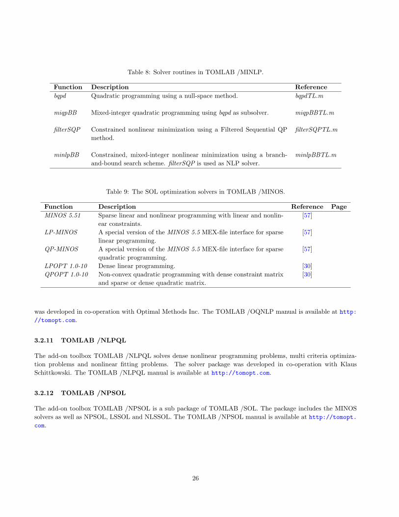
The add-on toolbox TOMLAB /MINLP provides solvers for continuous and mixed-integer quadratic programming(qp,miqp) and continuous and mixed-integer nonlinear constrained optimization (con, minlp).
All four solvers, written by Roger Fletcher and Sven Leyffer, University of Dundee, Scotland, are available insparse and dense versions. The solvers are listed in Table 8.
The TOMLAB /MINLP manual is available at http://tomopt.com.
3.2.9 TOMLAB /MINOS
Another set of Fortran solvers were developed by the Stanford Optimization Laboratory (SOL). Table 9 lists thesolvers included in TOMLAB /MINOS. The solvers are called using a set of MEX-file interfaces developed as partof TOMLAB. All functionality of the SOL solvers are available and changeable in the TOMLAB framework inMatlab.
3.2.10 TOMLAB /OQNLP
The add-on toolbox TOMLAB /OQNLP uses a multistart heuristic algorithm to find global optima of smoothconstrained nonlinear programs (NLPs) and mixed-integer nonlinear programs (MINLPs). The solver package
Function Description Referencebqpd Quadratic programming using a null-space method. bqpdTL.m
miqpBB Mixed-integer quadratic programming using bqpd as subsolver. miqpBBTL.m
filterSQP Constrained nonlinear minimization using a Filtered Sequential QPmethod.
filterSQPTL.m
minlpBB Constrained, mixed-integer nonlinear minimization using a branch-and-bound search scheme. filterSQP is used as NLP solver.
minlpBBTL.m
Table 9: The SOL optimization solvers in TOMLAB /MINOS.
Function Description Reference PageMINOS 5.51 Sparse linear and nonlinear programming with linear and nonlin-
ear constraints.[57]
LP-MINOS A special version of the MINOS 5.5 MEX-file interface for sparselinear programming.
[57]
QP-MINOS A special version of the MINOS 5.5 MEX-file interface for sparsequadratic programming.
[57]
LPOPT 1.0-10 Dense linear programming. [30]QPOPT 1.0-10 Non-convex quadratic programming with dense constraint matrix
and sparse or dense quadratic matrix.[30]
was developed in co-operation with Optimal Methods Inc. The TOMLAB /OQNLP manual is available at http://tomopt.com.
3.2.11 TOMLAB /NLPQL
The add-on toolbox TOMLAB /NLPQL solves dense nonlinear programming problems, multi criteria optimiza-tion problems and nonlinear fitting problems. The solver package was developed in co-operation with KlausSchittkowski. The TOMLAB /NLPQL manual is available at http://tomopt.com.
3.2.12 TOMLAB /NPSOL
The add-on toolbox TOMLAB /NPSOL is a sub package of TOMLAB /SOL. The package includes the MINOSsolvers as well as NPSOL, LSSOL and NLSSOL. The TOMLAB /NPSOL manual is available at http://tomopt.com.
The add-on toolbox TOMLAB /PENBMI solves linear semi-definite programming problems with linear and bilinearmatrix inequalities. The solvers are listed in Table 10. They are written in a combination of Matlab and C code.The TOMLAB /PENBMI manual is available at http://tomopt.com.
Table 10: Additional solvers in TOMLAB /PENSDP.
Function Description Reference Pagepenbmi Sparse and dense linear semi-definite programming using a penalty
algorithm.penfeas bmi Feasibility check of systems of linear matrix inequalities, using penbmi.
3.2.14 TOMLAB /PENSDP
The add-on toolbox TOMLAB /PENSDP solves linear semi-definite programming problems with linear matrixinequalities. The solvers are listed in Table 11. They are written in a combination of Matlab and C code. TheTOMLAB /PENSDP manual is available at http://tomopt.com.
Table 11: Additional solvers in TOMLAB /PENSDP.
Function Description Reference Pagepensdp Sparse and dense linear semi-definite programming using a penalty
algorithm.penfeas sdp Feasibility check of systems of linear matrix inequalities, using pensdp.
3.2.15 TOMLAB /SNOPT
The add-on toolbox TOMLAB /SNOPT is a sub package of TOMLAB /SOL. The package includes the MINOSsolvers as well as SNOPT and SQOPT. The TOMLAB /SNOPT manual is available at http://tomopt.com.
3.2.16 TOMLAB /SOL
The extension toolbox TOMLAB /SOL gives access to the complete set of Fortran solvers developed by theStanford Systems Optimization Laboratory (SOL). These solvers are listed in Table 9 and 12.
3.2.17 TOMLAB /SPRNLP
The add-on toolbox TOMLAB /SPRNLP solves large-scale nonlinear programming problems. SPRNLP is a state-of-the-art sequential quadratic programming (SQP) method, using an augmented Lagrangian merit function andsafeguarded line search. The solver package was developed in co-operation with Boeing Phantom Works. TheTOMLAB /SPRNLP package is described in a separate manual available at http://tomopt.com.
Table 12: The optimization solvers in the TOMLAB /SOL toolbox.
Function Description Reference PageNPSOL 5.02 Dense linear and nonlinear programming with linear and nonlinear
constraints.[34]
SNOPT 6.2-2 Large, sparse linear and nonlinear programming with linear andnonlinear constraints.
[33, 31]
SQOPT 6.2-2 Sparse convex quadratic programming. [32]NLSSOL 5.0-2 Constrained nonlinear least squares. NLSSOL is based on
NPSOL. No reference except for general NPSOL reference.[34]
LSSOL 1.05-4 Dense linear and quadratic programs (convex), and constrainedlinear least squares problems.
[29]
3.2.18 TOMLAB /XA
The add-on toolbox TOMLAB /XA solves large-scale linear, binary, integer and semi-continuous linear program-ming problems, as well as quadratic programming problems. The solver package was developed in co-operationwith Sunset Software Technology. The TOMLAB /XA package is described in a separate manual available athttp://tomopt.com.
3.2.19 TOMLAB /Xpress
The add-on toolbox TOMLAB /Xpress solves large-scale mixed-integer linear and quadratic programming prob-lems. The solver package was developed in co-operation with Dash Optimization Ltd. The TOMLAB /Xpresssolver package and interface are described in the html manual that comes with the installation package. There isalso a TOMLAB /Xpress manual available at http://tomopt.com.
To get a list of all available solvers, including Fortran, C and Matlab Optimization Toolbox solvers, for a certainsolvType, call the routine SolverList with solvType as argument. solvType should either be a string (’uc’, ’con’ etc.)or the corresponding solvType number as given in Table 1, page 11. For example, if wanting a list of all availablesolvers of solvType con, then
SolverList(’con’)
gives the output
>> SolverList(’con’);
Tomlab recommended choice for Constrained Nonlinear Programming (NLP)
npsol
Other solvers for NLP
Licensed:
nlpSolve
conSolve
sTrustr
constr
minos
snopt
fmincon
filterSQP
PDCO
PDSCO
Non-licensed:
NONE
Solvers also handling NLP
Licensed:
glcSolve
glcFast
glcCluster
rbfSolve
minlpBB
Non-licensed:
29
NONE
SolverList also returns two output arguments: all available solvers as a string matrix and a vector with thecorresponding solvType for each solver.
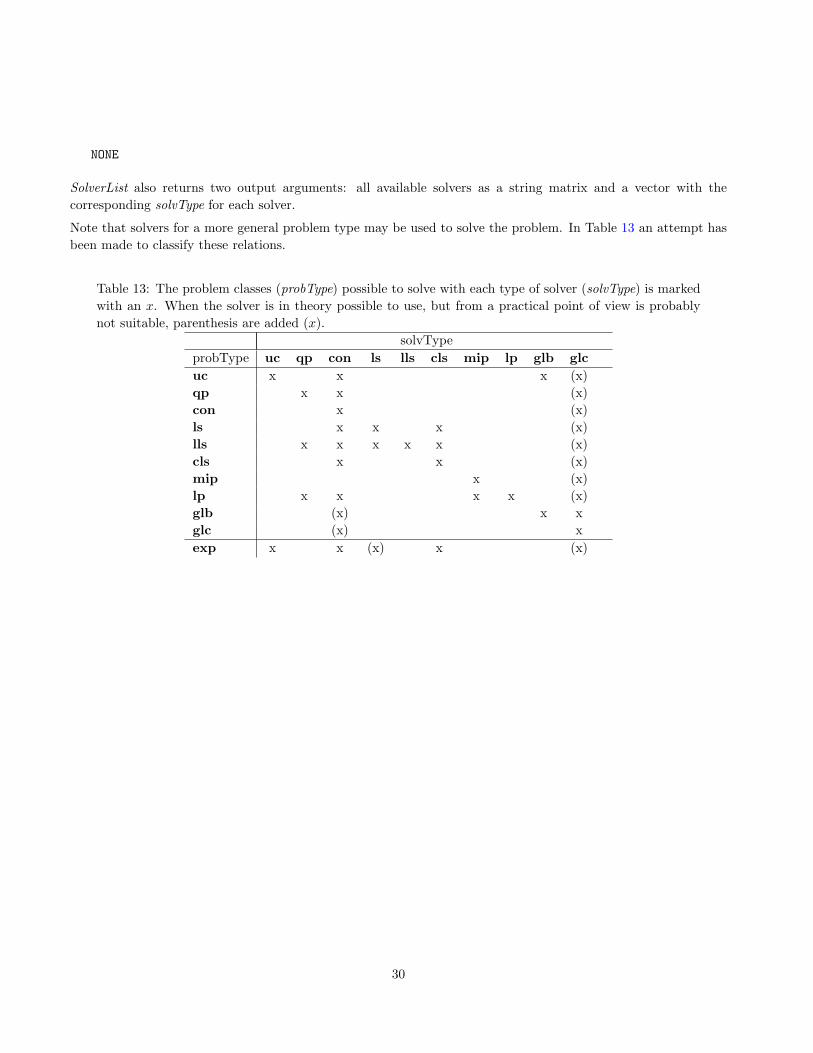
Note that solvers for a more general problem type may be used to solve the problem. In Table 13 an attempt hasbeen made to classify these relations.
Table 13: The problem classes (probType) possible to solve with each type of solver (solvType) is markedwith an x. When the solver is in theory possible to use, but from a practical point of view is probablynot suitable, parenthesis are added (x).
solvTypeprobType uc qp con ls lls cls mip lp glb glcuc x x x (x)qp x x (x)con x (x)ls x x x (x)lls x x x x x (x)cls x x (x)mip x (x)lp x x x x (x)glb (x) x xglc (x) xexp x x (x) x (x)
30
4 Defining Problems in TOMLAB
TOMLAB is based on the principle of creating a problem structure that defines the problem and includes allrelevant information needed for the solution of the user problem. One unified format is defined, the TOMLABformat. The TOMLAB format gives the user a fast way to setup a problem structure and solve the problem fromthe Matlab command line using any suitable TOMLAB solver.
TOMLAB also includes a modeling engine (or advanced Matlab class), TomSym, see Section 4.3. The package usesMatlab objects and operator overloading to capture Matlab procedures, and generates source code for derivativesof any order.
In this section follows a more detailed description of the TOMLAB format.
4.1 The TOMLAB Format
The TOMLAB format is a quick way to setup a problem and easily solve it using any of the TOMLAB solvers.The principle is to put all information in a Matlab structure, which then is passed to the solver, which extractsthe relevant information. The structure is passed to the user function routines for nonlinear problems, making ita convenient way to pass other types of information.
The solution process for the TOMLAB format has four steps:
1. Define the problem structure, often called Prob.
2. Call the solver or the universal driver routine tomRun.
3. Postprocessing, e.g. print the result of the optimization.
Step 1 could be done in several ways in TOMLAB. Recommended is to call one of the following routines dependenton the type of optimization problem, see Table 14.
Step 2, the solver call, is either a direct call, e.g. conSolve:
Prob = ProbCheck(Prob, ’conSolve’);
Result = conSolve(Prob);
or a call to the multi-solver driver routine tomRun, e.g. for constrained optimization:
Result = tomRun(’conSolve’, Prob);
Note that tomRun handles several input formats.
Step 3 could be a call to PrintResult.m:
PrintResult(Result);
The 3rd step could be included in Step 2 by increasing the print level to 1, 2 or 3 in the call to the driver routine
Result = tomRun(’conSolve’,Prob, 3);
See the different demo files that gives examples of how to apply the TOMLAB format: conDemo.m, ucDemo.m,qpDemo.m, lsDemo.m, lpDemo.m, mipDemo.m, glbDemo.m and glcDemo.m.
31
Table 14: Routines to create a problem structure in the TOMLAB format.
Prob = amplAssign( ... ) 1-3,7,8,11,12 For AMPL problems defined as nl -files.Prob = simAssign( ... ) 1,3-6,9-10 General routine, functions and constraints calculated at the same
time .
4.2 Modifying existing problems
It is possible to modify an existing Prob structure by editing elements directly, however this is not recommendedsince there are dependencies for memory allocation and problem sizes that the user may not be aware of.
There are a set of routines developed specifically for modifying linear constraints (do not modify directly, Prob.mLinneed to be set to a proper value if so). All the static information can be set with the following routines.
4.2.1 add A
PurposeAdds linear constraints to an existing problem.
Calling SyntaxProb = add A(Prob, A, b L, b U)
Description of Inputs
32
Prob Existing TOMLAB problem.A The additional linear constraints.b L The lower bounds for the new linear constraints.b U The upper bounds for the new linear constraints.
Description of Outputs
Prob Modified TOMLAB problem.
4.2.2 keep A
PurposeKeeps the linear constraints specified by idx.
Calling SyntaxProb = keep A(Prob, idx)
Description of Inputs
Prob Existing TOMLAB problem.idx The row indices to keep in the linear constraints.
Description of Outputs
Prob Modified TOMLAB problem.
4.2.3 remove A
PurposeRemoves the linear constraints specified by idx.
Calling SyntaxProb = remove A(Prob, idx)
Description of Inputs
Prob Existing TOMLAB problem.idx The row indices to remove in the linear constraints.
33
Description of Outputs
Prob Modified TOMLAB problem.
4.2.4 replace A
PurposeReplaces the linear constraints.
Calling SyntaxProb = replace A(Prob, A, b L, b U)
Description of Inputs
Prob Existing TOMLAB problem.A New linear constraints.b L Lower bounds for linear constraints.b U Upper bounds for linear constraints.
Description of Outputs
Prob Modified TOMLAB problem.
4.2.5 modify b L
PurposeModify lower bounds for linear constraints. If idx is not given b L will be replaced.
Calling SyntaxProb = modify b L(Prob, b L, idx)
Description of Inputs
Prob Existing TOMLAB problem.b L New lower bounds for the linear constraints.idx Indices for the modified constraint bounds (optional).
Description of Outputs
34
Prob Modified TOMLAB problem.
4.2.6 modify b U
PurposeModify upper bounds for linear constraints. If idx is not given b U will be replaced.
Calling SyntaxProb = modify b U(Prob, b U, idx)
Description of Inputs
Prob Existing TOMLAB problem.b U New upper bounds for the linear constraints.idx Indices for the modified constraint bounds (optional).
Description of Outputs
Prob Modified TOMLAB problem.
4.2.7 modify c
PurposeModify linear objective (LP/QP only).
Calling SyntaxProb = modify c(Prob, c, idx)
Description of Inputs
Prob Existing TOMLAB problem.c New linear coefficients.idx Indices for the modified linear coefficients (optional).
Description of Outputs
Prob Modified TOMLAB problem.
35
4.2.8 modify c L
PurposeModify lower bounds for nonlinear constraints. If idx is not given c L will be replaced.
Calling SyntaxProb = modify c L(Prob, c L, idx)
Description of Inputs
Prob Existing TOMLAB problem.c L New lower bounds for the nonlinear constraints.idx Indices for the modified constraint bounds (optional).
Description of Outputs
Prob Modified TOMLAB problem.
4.2.9 modify c U
PurposeModify upper bounds for nonlinear constraints. If idx is not given c U will be replaced.
Calling SyntaxProb = modify c U(Prob, c U, idx)
Description of Inputs
Prob Existing TOMLAB problem.c U New upper bounds for the nonlinear constraints.idx Indices for the modified constraint bounds (optional).
Description of Outputs
Prob Modified TOMLAB problem.
4.2.10 modify x 0
PurposeModify starting point. If x 0 is outside the bounds an error will be returned. If idx is not given x 0 will be replaced.
36
Calling SyntaxProb = modify x 0(Prob, x 0, idx)
Description of Inputs
Prob Existing TOMLAB problem.x 0 New starting points.idx Indices for the modified starting points (optional).
Description of Outputs
Prob Modified TOMLAB problem.
4.2.11 modify x L
PurposeModify lower bounds for decision variables. If idx is not given x L will be replaced. x 0 will be shifted if needed.
Calling SyntaxProb = modify x L(Prob, x L, idx)
Description of Inputs
Prob Existing TOMLAB problem.x L New lower bounds for the decision variables.idx Indices for the modified lower bounds (optional).
Description of Outputs
Prob Modified TOMLAB problem.
4.2.12 modify x U
PurposeModify upper bounds for decision variables. If idx is not given x U will be replaced. x 0 will be shifted if needed.
Calling SyntaxProb = modify x U(Prob, x U, idx)
37
Description of Inputs
Prob Existing TOMLAB problem.x U New upper bounds for the decision variables.idx Indices for the modified upper bounds (optional).
Description of Outputs
Prob Modified TOMLAB problem.
38
4.3 TomSym
For further information about TomSym, please visit http://tomsym.com/ - the pages contain detailed modelingexamples and real life applications. All illustrated examples are available in the folder /tomlab/tomsym/examples/in the TOMLAB installation. The modeling engine supports all problem types in TOMLAB with some minorexceptions.
A detailed function listing is available in Appendix C.
TomSym combines the best features of symbolic differentiation, i.e. produces source code with simplifications andoptimizations, with the strong point of automatic differentiation where the result is a procedure, rather than anexpression. Hence it does not grow exponentially in size for complex expressions.
Both forward and reverse modes are supported, however, reverse is default when computing the derivative withrespect to more than one variable. The command derivative results in forward mode, and derivatives in reversemode.
TomSym produces very efficient and fully vectorized code and is compatible with TOMLAB /MAD for situationswhere automatic differentiation may be the only option for parts of the model.
It should also be noted that TomSym automatically provides first and second order derivatives as well as problemsparsity patterns. With the use of TomSym the user no longer needs to code cumbersome derivative expressionsand Jacobian/Hessian sparsity patterns for most optimization and optimal control problems.
The main features in TomSym can be summarized with the following list:
• A full modeling environment in Matlab with support for most built-in mathematical operators.
• Automatically generates derivatives as Matlab code.
• A complete integration with PROPT (optimal control platform).
• Interfaced and compatible with MAD, i.e. MAD can be used when symbolic modeling is not suitable.
• Support for if, then, else statements.
• Automated code simplification for generated models.
• Ability to analyze most p-coded files (if code is vectorized).
4.3.1 Modeling
One of the main strength of TomSym is the ability to automatically and quickly compute symbolic derivatives ofmatrix expressions. The derivatives can then be converted into efficient Matlab code.
The matrix derivative of a matrix function is a fourth rank tensor - that is, a matrix each of whose entries isa matrix. Rather than using four-dimensional matrices to represent this, TomSym continues to work in twodimensions. This makes it possible to take advantage of the very efficient handling of sparse matrices in Matlab(not available for higher-dimensional matrices).
In order for the derivative to be two-dimensional, TomSym’s derivative reduces its arguments to one-dimensionalvectors before the derivative is computed. In the returned J , each row corresponds to an element of F , and eachcolumn corresponds to an element of X. As usual in Matlab, the elements of a matrix are taken in column-firstorder.
For vectors F and X, the resulting J is the well-known Jacobian matrix.
Observe that the TomSym notation is slightly different from commonly used mathematical notation. The notationused in tomSym was chosen to minimize the amount of element reordering needed to compute gradients for commonexpressions in optimization problems. It needs to be pointed out that this is different from the commonly usedmathematical notation, where the tensor ( dFdX ) is flattened into a two-dimensional matrix as it is written (There areactually two variations of this in common use - the indexing of the elements of X may or may not be transposed).
For example, in common mathematical notation, the so-called self derivative matrix (dXdX ) is a mn-by-mn square (ormm-by-nn rectangular in the non-transposed variation) matrix containing mn ones spread out in a random-lookingmanner. In tomSym notation, the self-derivative matrix is the mn-by-mn identity matrix.
The difference in notation only involves the ordering of the elements, and reordering the elements to a differentnotational convention should be trivial if tomSym is used to generate derivatives for applications other than forTOMLAB and PROPT.
Example:
>> toms y
>> toms 3x1 x
>> toms 2x3 A
>> f = (A*x).^(2*y)
f = tomSym(2x1):
(A*x).^(2*y)
>> derivative(f,A)
ans = tomSym(2x6):
(2*y)*setdiag((A*x).^(2*y-1))*kron(x’,eye(2))
In the above example, the 2x1 symbol f is differentiated with respect to the 2x3 symbol A. The result is a 2x6matrix, representing d(vec(f))
d(vec(A)) .
The displayed text is not necessarily identical to the m-code that will be generated from an expression. Forexample, the identity matrix is generated using speye in m-code, but displayed as eye (Derivatives tend to involvemany sparse matrices, which Matlab handles efficiently). The mcodestr command converts a tomSym object to aMatlab code string.
>> mcodestr(ans)
ans =
setdiag((2*y)*(A*x).^(2*y-1))*kron(x’,[1 0;0 1])
Observe that the command mcode and not mcodestr should be used when generating efficient production code.
4.3.2 Ezsolve
TomSym provides the function ezsolve, which needs minimal input to solve an optimization problem: only theobjective function and constraints. For example, the miqpQG example from the tomlab quickguide can be reducedto the following:
40
toms integer x
toms y
objective = -6*x + 2*x^2 + 2*y^2 - 2*x*y;
constraints = {x+y<=1.9,x>=0, y>=0};
solution = ezsolve(objective,constraints)
Ezsolve calls tomDiagnose to determine the problem type, getSolver to find an appropriate solver, then sym2prob,tomRun and getSoluton in sequence to obtain the solution.
Advanced users might not use ezsolve, and instead call sym2prob and tomRun directly. This provides for thepossibility to modify the Prob struct and set flags for the solver.
4.3.3 Usage
TomSym, unlike most other symbolic algebra packages, focuses on vectorized notation. This should be familiarto Matlab users, but is very different from many other programming languages. When computing the derivativeof a vector-valued function with respect to a vector valued variable, tomSym attempts to give a derivative asvectorized Matlab code. However, this only works if the original expressions use vectorized notation. For example:
toms 3x1 x
f = sum(exp(x));
g = derivative(f,x);
results in the efficient g = exp(x)′. In contrast, the mathematically equivalent but slower code:
toms 3x1 x
f = 0;
for i=1:length(x)
f = f+exp(x(i));
end
g = derivative(f,x);
results in g = (exp(x(1)) ∗ [100] + exp(x(2)) ∗ [010]) + exp(x(3)) ∗ [001] as each term is differentiated individually.Since tomSym has no way of knowing that all the terms have the same format, it has to compute the symbolicderivative for each one. In this example, with only three iterations, that is not really a problem, but large for-loopscan easily result in symbolic calculations that require more time than the actual numeric solution of the underlyingoptimization problem.
It is thus recommended to avoid for-loops as far as possible when working with tomSym.
Because tomSym computes derivatives with respect to whole symbols, and not their individual elements, it is alsoa good idea not to group several variables into one vector, when they are mostly used individually. For example:
toms 2x1 x
f = x(1)*sin(x(2));
g = derivative(f,x);
41
results in g = sin(x(2)) ∗ [10] + x(1) ∗ (cos(x(2)) ∗ [01]). Since x is never used as a 2x1 vector, it is better to usetwo independent 1x1 variables:
toms a b
f = a*sin(b);
g = derivative(f,[a; b]);
which results in g = [sin(b) a ∗ cos(b)]. The main benefit here is the increased readability of the auto-generatedcode, but there is also a slight performance increase (Should the vector x later be needed, it can of course easilybe created using the code x = [a; b]).
4.3.4 Scaling variables
Because tomSym provides analytic derivatives (including second order derivatives) for the solvers, badly scaledproblems will likely be less problematic from the start. To further improve the model, tomSym also makes itvery easy to manually scale variables before they are presented to the solver. For example, assuming that anoptimization problem involves the variable x which is of the order of magnitude 1e6, and the variable y, which isof the order of 1e− 6, the code:
toms xScaled yScaled
x = 1e+6*xScaled;
y = 1e-6*yScaled;
will make it possible to work with the tomSym expressions x and y when coding the optimization problem, whilethe solver will solve for the symbols xScaled and yScaled, which will both be in the order of 1. It is even possibleto provide starting guesses on x and y (in equation form), because tomSym will solve the linear equation to obtainstarting guesses for the underlying xScaled and yScaled.
The solution structure returned by ezsolve will of course only contain xScaled and yScaled, but numeric values forx and y are easily obtained via, e.g. subs(x,solution).
4.3.5 SDP/LMI/BMI interface
An interface for bilinear semidefinite problems is included with tomSym. It is also possible to solve nonlinearproblems involving semidefinite constraints, using any nonlinear solver (The square root of the semidefinte matrixis then introduced as an extra set of unknowns).
See the examples optimalFeedbackBMI and example sdp.
4.3.6 Interface to MAD and finite differences
If a user function is incompatible with tomSym, it can still be used in symbolic computations, by giving it a”wrapper”. For example, if the cos function was not already overloaded by tomSym, it would still be possible todo the equivalent of cos(3*x) by writing feval(’cos’,3*x).
MAD then computes the derivatives when the Jacobian matrix of a wrapped function is needed. If MAD isunavailable, or unable to do the job, numeric differentiation is used.
Second order derivatives cannot be obtained in the current implementation.
42
It is also possible to force the use of automatic or numerical differentiation for any function used in the code. Thefollow examples shows a few of the options available:
toms x1 x2
alpha = 100;
% 1. USE MAD FOR ONE FUNCTION.
% Create a wrapper function. In this case we use sin, but it could be any
% MAD supported function.
y = wrap(struct(’fun’,’sin’,’n’,1,’sz1’,1,’sz2’,1,’JFuns’,’MAD’),x1/x2);
f = alpha*(x2-x1^2)^2 + (1-x1)^2 + y;
% Setup and solve the problem
c = -x1^2 - x2;
con = {-1000 <= c <= 0
-10 <= x1 <= 2
-10 <= x2 <= 2};
x0 = {x1 == -1.2
x2 == 1};
solution1 = ezsolve(f,con,x0);
% 2. USE MAD FOR ALL FUNCTIONS.
options = struct;
options.derivatives = ’automatic’;
f = alpha*(x2-x1^2)^2 + (1-x1)^2 + sin(x1/x2);
solution2 = ezsolve(f,con,x0,options);
% 3. USE FD (Finite Differences) FOR ONE FUNCTIONS.
% Create a new wrapper function. In this case we use sin, but it could be
% any function since we use numerical derivatives.
y = wrap(struct(’fun’,’sin’,’n’,1,’sz1’,1,’sz2’,1,’JFuns’,’FDJac’),x1/x2);
The code generation function detects sub-expressions that occur more than once, and optimizes by creating tem-porary variables for those since it is very common for a function to share expressions with its derivative, or for thederivative to contain repeated expressions.
Note that it is not necessary to complete code generation in order to evaluate a tomSym object numerically. Thesubs function can be used to replace symbols by their numeric values, resulting in an evaluation.
TomSym also automatically implements algebraic simplifications of expressions. Among them are:
• Multiplication by 1 is eliminated: 1 ∗A = A
• Addition/subtraction of 0 is eliminated: 0 +A = A
• All-same matrices are reduced to scalars: [3; 3; 3] + x = 3 + x
• Scalars are moved to the left in multiplications: A ∗ y = y ∗A
• Scalars are moved to the left in addition/subtraction: A− y = −y +A
• Expressions involving element-wise operations are moved inside setdiag: setdiag(A)+setdiag(A) = setdiag(A+A)
• Inverse operations cancel: sqrt(x)2 = x
• Multiplication by inverse cancels: A ∗ inv(A) = eye(size(A))
• Subtraction of self cancels: A−A = zeros(size(A))
• Among others...
Except in the case of scalar-matrix operations, tomSym does not reorder multiplications or additions, which meansthat some expressions, like (A+B)-A will not be simplified (This might be implemented in a later version, butmust be done carefully so that truncation errors are not introduced).
Simplifications are also applied when using subs. This makes it quick and easy to handle parameterized problems.For example, if an intricate optimization problem is to be solved for several values of a parameter a, then one
44
might first create the symbolic functions and gradients using a symbolic a, and then substitute the different values,and generate m-code for each substituted function. If some case, like a = 0 results in entire sub-expressions beingeliminated, then the m-code will be shorter in that case.
It is also possible to generate complete problems with constants as decision variables and then change the boundsfor these variables to make them ”real constants”. The backside of this is that the problem will be slightly larger,but the problem only has to be generated once.
The following problem defines the variable alpha as a toms, then the bounds are adjusted for alpha to solve theproblem for all alphas from 1 to 100.
toms x1 x2
% Define alpha as a toms although it is a constant
toms alpha
% Setup and solve the problem
f = alpha*(x2-x1^2)^2 + (1-x1)^2;
c = -x1^2 - x2;
con = {-1000 <= c <= 0
-10 <= x1 <= 2
-10 <= x2 <= 2};
x0 = {x1 == -1.2; x2 == 1};
Prob = sym2prob(f,con,x0);
% Now solve for alpha = 1:100, while reusing x_0
obj = zeros(100,1);
for i=1:100
Prob.x_L(Prob.tomSym.idx.alpha) = i;
Prob.x_U(Prob.tomSym.idx.alpha) = i;
Prob.x_0(Prob.tomSym.idx.alpha) = i;
Result = tomRun(’snopt’, Prob, 1);
Prob.x_0 = Result.x_k;
obj(i) = Result.f_k;
end
4.3.8 Special functions
TomSym adds some functions that duplicates the functionality of Matlab, but that are more suitable for symbolictreatment. For example:
• setDiag and getDiag - Replaces some uses of Matlab’s diag function, but clarifies whether diag(x) means”create a matrix where the diagonal elements are the elements of x” or ”extract the main diagonal from thematrix x”.
• subsVec applies an expression to a list of values. The same effect can be achieved with a for-loop, butsubsVec gives more efficient derivatives.
45
• ifThenElse - A replacement for the if ... then ... else constructs (See below).
If ... then ... else:
A common reason that it is difficult to implement a function in tomSym is that it contains code like the following:
if x<2
y = 0;
else
y = x-2;
end
Because x is a symbolic object, the expression x < 2 does not evaluate to true or false, but to another symbolicobject.
In tomSym, one should instead write:
y = ifThenElse(x<2,0,x-2)
This will result in a symbolic object that contains information about both the ”true” and the ”false” scenario.However, taking the derivative of this function will result in a warning, because the derivative is not well-definedat x = 2.
The ”smoothed” form:
y = ifThenElse(x<2,0,x-2,0.1)
yields a function that is essentially the same for abs(x− 2) > 3 ∗ 0.1, but which follows a smooth curve near x = 2,ensuring that derivatives of all orders exist. However, this introduces a local minimum which did not exist in theoriginal function, and invalidates the convexity.
It is recommended that the smooth form ifThenElse be used for nonlinear problems whenever it replaces a dis-continuous function. However, for convex functions (like the one above) it is usually better to use code that helpstomSym know that convexity is preserved. For example, instead of the above ifThenElse(x < 2, 0, x− 2, 0.1), theequivalent max(0, x− 2) is preferred.
4.3.9 Procedure vs parse-tree
TomSym works with procedures. This makes it different from many symbolic algebra packages, that mainly workwith parse-trees.
In optimization, it is not uncommon for objectives and constraints to be defined using procedures that involveloops. TomSym is built to handle these efficiently. If a function is defined using many intermediate steps, thentomSym will keep track of those steps in an optimized procedure description. For example, consider the code:
toms x
y = x*x;
z = sin(y)+cos(y);
In the tomSym object z, there is now a procedure, which looks something like:
46
temp = x*x;
result = cos(temp)+sin(temp);
Note: It is not necessary to use the intermediate symbol y. TomSym, automatically detects duplicated expressions,so the code sin(x*x)+cos(x*x) would result in the same optimized procedure for z.
On the other hand, the same corresponding code using the symbolic toolbox:
syms x
y = x*x;
z = sin(y)+cos(y);
results in an object z that contains cos(x2) + sin(x2), resulting in a double evaluation of x2.
This may seem like a small difference in this simplified example, but in real-life applications, the difference can besignificant.
Numeric stability:
For example, consider the following code, which computes the Legendre polynomials up to the 100th order intomSym (The calculation takes about two seconds on a modern computer).
toms x
p{1}=1;
p{2}=x;
for i=1:99
p{i+2} = ((2*i+1)*x.*p{i+1}-i*p{i})./(i+1);
end
Replacing ”toms” by ”syms” on the first line should cause the same polynomials to be computed using Mathwork’sSymbolic Toolbox. But after a few minutes, when only about 30 polynomials have been computed, the programcrashes as it fails to allocate more memory. This is because the expression grows exponentially in size. Tocircumvent the problem, the expression must be algebraically simplified after each step. The following codesucceeds in computing the 100 polynomials using the symbolic toolbox.
However, the simplification changes the way in which the polynomial is computed. This is clearly illustrated if weinsert x = 1 into the 100th order polynomial. This is accomplished by using the command subs(p101,x,1) for boththe tomSym and the Symbolic Toolbox expressions. TomSym returns the result 1.0000, which is correct. Thesymbolic toolbox, on the other hand, returns 2.6759e+ 020, which is off by 20 orders of magnitude. The reason isthat the ”simplified” symbolic expressions involves subtracting very large numbers. Note: It is of course possible toget correct results from the Symbolic Toolbox using exact arithmetic instead of machine-precision floating-point,but at the cost of much slower evaluation.
47
In tomSym, there are also simplifications, for example identifying identical sub-trees, or multiplication by zero,but the simplifications are not as extensive, and care is taken to avoid simplifications that can lead to truncationerrors. Thus, an expression computed using tomSym should be exactly as stable (or unstable) as the algorithmused to generate it.
Another example:
The following code, iteratively defines q as a function of the tomSym symbol x, and computes its derivative:
And this example only had four iterations of the loop. Increasing the number of iterations, the Symbolic toolboxexpressions quickly becomes unmanageable, while the tomSym procedure only grows linearly.
4.3.10 Problems and error messages
• Warning: Directory c:\Temp\tp563415 could not be removed (or similar). When tomSym is usedto automatically create m-code it places the code in a temporary directory given by Matlab’s tempnamefunction. Sometimes Matlab chooses a name that already exists, which results in this error message (Thetemporary directory is cleared of old files regularly by most modern operating systems. Otherwise thetemporary Matlab files can easily be removed manually).
• Attempting to call SCRIPT as a function (or similar). Due to a bug in the Matlab syntax, theparser cannot know if f(x) is a function call or the x:th element of the vector f. Hence, it has to guess. TheMatlab parser does not understand that toms creates variables, so it will get confused if one of the names ispreviously used by a function or script (For example, ”cs” is a script in the systems identification toolbox).Declaring toms cs and then indexing cs(1) will work at the Matlab prompt, but not in a script. The bug canbe circumvented by assigning something to each variable before calling toms.
4.3.11 Example
A TomSym model is to a great extent independent upon the problem type, i.e. a linear, nonlinear or mixed-integernonlinear model would be modeled with about the same commands. The following example illustrates how toconstruct and solve a MINLP problem using TomSym.
The TomSym engine automatically completes the separation of simple bounds, linear and nonlinear constraints.
50
5 Solving Linear, Quadratic and Integer Programming Problems
This section describes how to define and solve linear and quadratic programming problems, and mixed-integerlinear programs using TOMLAB. Several examples are given on how to proceed, depending on if a quick solutionis wanted, or more advanced tests are needed. TOMLAB is also compatible with MathWorks Optimization TB.See Appendix E for more information and test examples.
The test examples and output files are part of the standard distribution of TOMLAB, available in directoryusersguide, and all tests can be run by the user. There is a file RunAllTests that goes through and runs all testsfor this section.
Also see the files lpDemo.m, qpDemo.m, and mipDemo.m, in the directory examples, where in each file a set ofsimple examples are defined. The examples may be ran by giving the corresponding file name, which displays amenu, or by running the general TOMLAB help routine tomHelp.m.
5.1 Linear Programming Problems
The general formulation in TOMLAB for a linear programming problem is
minx
f(x) = cTx
s/txL ≤ x ≤ xU ,
bL ≤ Ax ≤ bU
(12)
where c, x, xL, xU ∈ Rn, A ∈ Rm1×n, and bL, bU ∈ Rm1 . Equality constraints are defined by setting the lowerbound equal to the upper bound, i.e. for constraint i: bL(i) = bU (i).
To illustrate the solution of LPs consider the simple linear programming test problem
minx1,x2
f(x1, x2) = −7x1 − 5x2
s/t x1 + 2x2 ≤ 64x1 + x2 ≤ 12x1, x2 ≥ 0
(13)
named LP Example.
The following statements define this problem in Matlab
File: tomlab/usersguide/lpExample.m
Name = ’lptest’;
c = [-7 -5]’; % Coefficients in linear objective function
A = [ 1 2
4 1 ]; % Matrix defining linear constraints
b_U = [ 6 12 ]’; % Upper bounds on the linear inequalities
x_L = [ 0 0 ]’; % Lower bounds on x
% x_min and x_max are only needed if doing plots
x_min = [ 0 0 ]’;
x_max = [10 10 ]’;
51
% b_L, x_U and x_0 have default values and need not be defined.
% It is possible to call lpAssign with empty [] arguments instead
b_L = [-inf -inf]’;
x_U = [];
x_0 = [];
5.1.1 A Quick Linear Programming Solution
The quickest way to solve this problem is to define the following Matlab statements using the TOMLAB format:
File: tomlab/usersguide/lpTest1.m
lpExample;
Prob = lpAssign(c, A, b_L, b_U, x_L, x_U, x_0, ’lpExample’);
Result = tomRun(’lpSimplex’, Prob, 1);
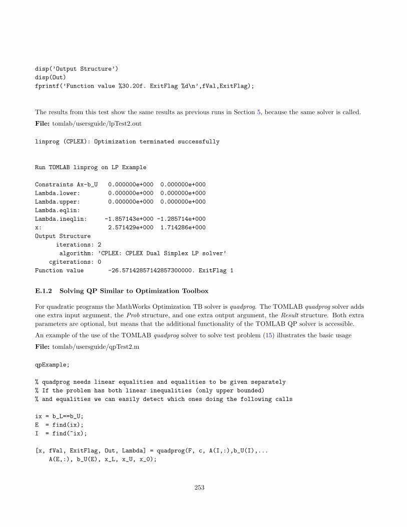
lpAssign is used to define the standard Prob structure, which TOMLAB always uses to store all information abouta problem. The three last parameters could be left out. The upper bounds will default be Inf, and the problemname is only used in the printout in PrintResult to make the output nicer to read. If x 0, the initial value, is leftout, an initial point is found by lpSimplex solving a feasible point (Phase I) linear programming problem. In thistest the given x 0 is empty, so a Phase I problem must be solved. The solution of this problem gives the followingoutput to the screen
CPU time: 0.046800 sec. Elapsed time: 0.019000 sec.
Having defined the Prob structure is it easy to call any solver that can handle linear programming problems,
Result = tomRun(’qpSolve’, Prob, 1);
Even a nonlinear solver may be used.
Result = tomRun(’nlpSolve’,Prob, 3);
All TOMLAB solvers may either be called directly, or by using the driver routine tomRun, as in this case.
52
5.2 Quadratic Programming Problems
The general formulation in TOMLAB for a quadratic programming problem is
minx
f(x) = 12x
TFx+ cTx
s/txL ≤ x ≤ xU ,
bL ≤ Ax ≤ bU
(14)
where c, x, xL, xU ∈ Rn, F ∈ Rn×n, A ∈ Rm1×n, and bL, bU ∈ Rm1 . Equality constraints are defined by setting thelower bound equal to the upper bound, i.e. for constraint i: bL(i) = bU (i). Fixed variables are handled the sameway.
To illustrate the solution of QPs consider the simple quadratic programming test problem
minx
f(x) = 4x21 + 1x1x2 + 4x2
2 + 3x1 − 4x2
s/t x1 + x2 ≤ 5x1 − x2 = 0x1 ≥ 0x2 ≥ 0,
(15)
named QP Example. The following statements define this problem in Matlab.
File: tomlab/usersguide/qpExample.m
Name = ’QP Example’; % File qpExample.m
F = [ 8 1 % Matrix F in 1/2 * x’ * F * x + c’ * x
1 8 ];
c = [ 3 -4 ]’; % Vector c in 1/2 * x’ * F * x + c’ * x
A = [ 1 1 % Constraint matrix
1 -1 ];
b_L = [-inf 0 ]’; % Lower bounds on the linear constraints
b_U = [ 5 0 ]’; % Upper bounds on the linear constraints
x_L = [ 0 0 ]’; % Lower bounds on the variables
x_U = [ inf inf ]’; % Upper bounds on the variables
CPU time: 0.046800 sec. Elapsed time: 0.037000 sec.
qpAssign is used to define the standard Prob structure, which TOMLAB always uses to store all information abouta problem. The three last parameters could be left out. The upper bounds will default be Inf, and the problemname is only used in the printout in PrintResult to make the output nicer to read. If x 0, the initial value, is leftout, a initial point is found by qpSolve solving a feasible point (Phase I) linear programming problem calling theTOMLAB lpSimplex solver. In fact, the output shows that the given x0 = (0,−1)T was rejected because it wasinfeasible, and instead a Phase I solution lead to the initial point x0 = (0, 0)T .
54
5.3 Mixed-Integer Programming Problems
This section describes how to solve mixed-integer programming problems efficiently using TOMLAB. To illustratethe solution of MIPs consider the simple knapsack 0/1 test problem Weingartner 1, which has 28 binary variablesand two knapsacks. The problem is defined
Prob.Solver.Alg = 2; % Depth First, then Breadth search
Prob.optParam.IterPrint = 0;
Prob.PriLev = 1;
Result = tomRun(’mipSolve’, Prob, 0);
To make it easier to see all variable settings, the first lines define the needed variables. Several of them arejust empty arrays, and could be directly set as empty in the call to mipAssign. mipAssign is used to define thestandard Prob structure, which TOMLAB always uses to store all information about a problem. After mipAssignhas defined the structure Prob it is then easy to set or change fields in the structure. The solver mipSolve is usingthree different strategies to search the branch-and-bound tree. The default is the Depth first strategy, which isalso the result if setting the field Solver.Alg as zero. Setting the field as one gives the Breadth first strategy andsetting it as two gives the Depth first, then breadth search strategy. In the example our choice is the last strategy.The number of iterations might be many, thus the maximal number of iterations must be increased, the fieldoptParam.MaxIter.
57
Tests show two ways to improve the convergence of MIP problems. One is to define a priority order in whichthe different non-integer variables are selected as variables to branch on. The field MIP.VarWeight is used toset priority numbers for each variable. Note that the lower the number, the higher the priority. In our test casethe coefficients of the objective function is used as priority weights. The other way to improve convergence is touse a heuristic. For binary variables a simple knapsack heuristic is implemented in mipSolve. Setting the fieldMIP.KNAPSACK as true instructs mipSolve to use the heuristic.
Running the four different tests on the knapsack problem gives the following output to the screen
Note that there is a large difference in the number of iterations if the additional heuristic and priorities are used.Similar results are obtained if running the other two tree search strategies.
59
6 Solving Unconstrained and Constrained Optimization Problems
This section describes how to define and solve unconstrained and constrained optimization problems. Severalexamples are given on how to proceed, depending on if a quick solution is wanted, or more advanced runs areneeded. See Appendix E for more information on your external solvers.
All demonstration examples that are using the TOMLAB format are collected in the directory examples. It is alsopossible to run each example separately. The examples relevant to this section are ucDemo and conDemo. Thefull path to these files are always given in the text. Throughout this section the test problem Rosenbrock’s banana,
minx
f(x) = α(x2 − x2
1
)2 + (1− x1)2
s/t−10 ≤ x1 ≤ 2−10 ≤ x2 ≤ 2
(17)
is used to illustrate the solution of unconstrained problems. The standard value is α = 100. In this formulationsimple bounds are added on the variables, and also constraints in illustrative purpose. This problem is calledRB BANANA in the following descriptions to avoid mixing it up with problems already defined in the problemdefinition files.
6.1 Defining the Problem in Matlab m-files
TOMLAB demands that the general nonlinear problem is defined in Matlab m-files, and not given as an input textstring. A file defining the function to be optimized must always be supplied. For linear constraints the constraintcoefficient matrix and the right hand side vector are given directly. Nonlinear constraints are defined in a separatefile. First order derivatives and second order derivatives, if available, are stored in separate files, both functionderivatives and constraint derivatives.
TOMLAB is compatible with MathWorks Optimization TB, which in various ways demands both functions, deriva-tives and constraints to be returned by the same function. TOMLAB handle all this by use of interface routines,hidden for the user.
It is generally recommended to use the TOMLAB format instead, because having defined the files in this format,all MathWorks Optimization TB solvers are accessible through the TOMLAB multi-solver driver routines.
The rest of this section shows how to make the m-files for the cases of unconstrained and constrained optimization.In Section 6.2 and onwards similar m-files are used to solve unconstrained optimization using the TOMLAB format.
The most simple way to write the m-file to compute the function value is shown for the example in (17) assumingα = 100:
File: tomlab/usersguide/rbbs f.m
% rbbs_f - function value for Constrained Rosenbrocks Banana
%
% function f = rbbs_f(x)
function f = rbbs_f(x)
f = 100*(x(2)-x(1)^2)^2 + (1-x(1))^2;
Running TOMLAB it is recommended to use a more general format for the m-files, adding one extra parameter,
60
the Prob problem definition structure described in detail in Appendix A. TOMLAB will handle the simpler formatalso, but the more advanced features of TOMLAB are not possible to use.
If using this extra parameter, then any information needed in the low-level function computation routine may besent as fields in this structure. For single parameter values, like the above α parameter in the example, the fieldProb.user is recommended.
Using the above convention, then the new m-file for the example in (17) is defined as
File: tomlab/usersguide/rbb f.m
% rbb_f - function value for Rosenbrocks Banana, Problem RB BANANA
%
% function f = rbb_f(x, Prob)
function f = rbb_f(x, Prob)
alpha = Prob.user.alpha;
f = alpha*(x(2)-x(1)^2)^2 + (1-x(1))^2;
The value in the field Prob.user is the α value. It is defined before calling the solver by explicit setting the Probstructure. In a similar way the gradient routine is defined as
File: tomlab/usersguide/rbb g.m
% rbb_g - gradient vector for Rosenbrocks Banana, Problem RB BANANA
%
% function g = rbb_g(x, Prob)
function g = rbb_g(x, Prob)
alpha = Prob.user.alpha;
g = [-4*alpha*x(1)*(x(2)-x(1)^2)-2*(1-x(1)); 2*alpha*(x(2)-x(1)^2)];
If the gradient routine is not supplied, TOMLAB will use finite differences (or automatic differentiation) if thegradient vector is needed for the particular solver. In this case it is also easy to compute the Hessian matrix, whichgives the following code
File: tomlab/usersguide/rbb H.m
% rbb_H - Hessian matrix for Rosenbrocks Banana, Problem RB BANANA
%
% function H = crbb_H(x, Prob)
function H = rbb_H(x, Prob)
alpha = Prob.user.alpha;
61
H = [ 12*alpha*x(1)^2-4*alpha*x(2)+2 , -4*alpha*x(1);
-4*alpha*x(1) , 2*alpha ];
If the Hessian routine is not supplied, TOMLAB will use finite differences (or automatic differentiation) if theHessian matrix is needed for the particular solver. Often a positive-definite approximation of the Hessian matrixis estimated during the optimization , and the second derivative routine is then not used.
If using the constraints defined for the example in (17) then a constraint routine needs to defined for the singlenonlinear constraint, in this case
File: tomlab/usersguide/rbb c.m
% rbb_c - nonlinear constraint vector for Rosenbrocks Banana, Problem RB BANANA
%
% function c = rbb_c(x, Prob)
function cx = rbb_c(x, Prob)
cx = -x(1)^2 - x(2);
The constraint Jacobian matrix is also of interest and is defined as
File: tomlab/usersguide/rbb dc.m
% rbb_dc - nonlinear constraint gradient matrix
% for Rosenbrocks Banana, Problem RB BANANA
%
% function dc = crbb_dc(x, Prob)
function dc = rbb_dc(x, Prob)
% One row for each constraint, one column for each variable.
dc = [-2*x(1),-1];
If the constraint Jacobian routine is not supplied, TOMLAB will use finite differences (or automatic differentiation)to estimate the constraint Jacobian matrix if it is needed for the particular solver.
The solver nlpSolve is also using the second derivatives of the constraint vector. The result is returned as aweighted sum of the second derivative matrices with respect to each constraint vector element, the weights beingthe Lagrange multipliers supplied as input to the routine. For the example problem the routine is defined as
File: tomlab/usersguide/rbb d2c.m
% rbb_d2c - The second part of the Hessian to the Lagrangian function for the
% nonlinear constraints for Rosenbrocks Banana, Problem RB BANANA, i.e.
% The only nonzero element in the second derivative matrix for the single
% constraint is the (1,1) element, which is a constant -2.
d2c = lam(1)*[-2 0; 0 0];
6.1.1 Communication between user routines
It is often the case that mathematical expressions that occur in the function computation also is part of thegradient and Hessian computation. If these operations are costly it is natural to avoid recomputing these andreuse them when computing the gradient and Hessian.
The function routine is always called before the gradient routine in TOMLAB, and the gradient routine is alwayscalled before the Hessian routine. The constraint routine is similarly called before the computation of the constraintgradient matrix. However, the TOM solvers call the function before the constraint routine, but the SOL solversdo the reverse.
Thus it is safe to use global variables to communicate information from the function routine to the gradient andHessian, and similarly from the constraint routine to the constraint gradient routine. Any non-conflicting namecould be used as global variable, see Table 154 in Appendix D to find out which names are in use. However, therecommendation is to always use a predefined global variable named US A for this communication. TOMLAB isdesigned to handle recursive calls, and any use of new global variables may cause conflicts. The variable US A(and also US B) is automatically saved in a stack, and any level of recursions may safely be used. The user is freeto use US A both as variable, and as a structure. If much information is to be communicated, defining US A as astructure makes it possible to send any amount of information between the user routines.
In the examples directory the constrained optimization example in conDemo is using the defined functions con1 f,con1 g and con1 H. They include an example of communicating one exponential expression between the routines.
The lsDemo example file in the examples directory communicates two exponential expressions between ls1 r andls1 J with the use of US A and US B. In ls1 r the main part is
...
global US_A
t = Prob.LS.t(:);
% Exponential computations takes time, and may be done once, and
% reused when computing the Jacobian
US_A = exp(-x(1)*t);
US_B = exp(-x(2)*t);
63
r = K*x(1)*(US_B - US_A) / (x(3)*(x(1)-x(2))) - Prob.LS.y;
In ls1 J then US A is used
...
global US_A
% Pick up the globally saved exponential computations
e1 = US_A;
e2 = US_B;
% Compute the three columns in the Jacobian, one for each of variable
J = a * [ t.*e1+(e2-e1)*(1-1/b), -t.*e2+(e2-e1)/b, (e1-e2)/x(3)];
For more discussions on global variables and the use of recursive calls in TOMLAB, see Appendix D.
In the following sections it is described how to setup problems in TOMLAB and use the defined m-files. Firstcomes the simplest way, to use the TOMLAB format.
6.2 Unconstrained Optimization Problems
The use of the TOMLAB format is best illustrated by examples
The following is the first example in the ucDemo demonstration file. It shows an example of making a call toconAssign to create a structure in the TOMLAB format, and solve the problem with a call to ucSolve.
In its more general form conAssign is used to define constrained problems. It also takes as input the nonzeropattern of the Hessian matrix, stored in the matrix HessPattern. In this case all elements of the Hessian matrixare nonzero, and either HessPattern is set as empty or as a matrix with all ones. Also the parameter pSepFuncshould be set. It defines if the objective function is partially separable, see Section 14.5. Setting this parameterempty (the default), then this property is not used. In the above example the call would be
...
HessPattern = ones(2,2); % The pattern of nonzeros
pSepFunc = []; % No partial separability used
% conAssign is used to generate the TOMLAB problem structure
Also see the other examples in ucDemo on how to solve the problem, when gradients routines are not present, andnumerical differentiation must be used. An example on how to solve a sequence of problems is also presented.
If the gradient is not possible to define one just sets the corresponding gradient function name empty.
The example uc3Demo in file ucDemo show how to solve a sequence of problems in TOMLAB, in this case changingthe steepness parameter α in (17). It is important to point out that it is only necessary to define the Prob structureonce and then just change the varying parameters, in this case the α value. The α value is sent to the user routinesusing the field user in the Prob structure. Any field in the Prob structure could be used that is not conflicting withthe predefined fields. In this example the a vector of Result structures are saved for later preprocessing.
When wanting to solve a problem by a direct call to an optimization routine there are two possible ways of doingit. The difference is in the way the problem dependent parameters are defined. The most natural way is to use aInit File, like the predefined TOMLAB Init Files � prob (e.g. uc prob if the problem is of the type unconstrained)to define those parameters. The other way is to call the routine conAssign. In this subsection, examples of twodifferent approaches are given.
First, solve the problem RB BANANA in (17) as an unconstrained problem. In this case, define the problem inthe files ucnew prob, ucnew f, ucnew g and ucnew H. Using the problem definition files in the working directorysolve the problem and print the result by the following calls.
File: tomlab/usersguide/ucnewSolve1.m
probFile = ’ucnew_prob’; % Problem definition file.
Now, solve the same problem as in the example above but define the parameters x 0, x L and x L by calling theroutine conAssign. Note that in this case the file ucnew prob is not used, only the files ucnew f and ucnew g. Thefile ucnew H is not needed because a quasi-Newton BFGS algorithm is used.
File: tomlab/usersguide/ucnewSolve2.m
x_0 = [-1.2;1]; % Starting values for the optimization.
The first two constraints are simple bounds, the third is a linear equality constraint, because lower and upperbounds are the same. The last two constraints are nonlinear inequality constraints. To solve the problem, definethe following statements, available as con1Demo in file conDemo.
66
Name = ’Exponential problem III’;
A = [1 1]; % One linear constraint
b_L = 0; % Lower bound on linear constraint
b_U = 0; % b_L == b_U implies equality
c_L = [1.5;-10] % Two nonlinear inequality constraints
c_U = []; % Empty means Inf (default) for the two constraints
x_0 = [-5;5]; % Initial value for x
x_L = [-10;-10]; % Lower bounds on x
x_U = [10;10]; % Upper bounds on x
fLowBnd = 0; % A lower bound on the optimal function value
x_min = [-2;-2]; % Used for plotting, lower bounds
x_max = [4;4]; % Used for plotting, upper bounds
x_opt=[-3.162278, 3.162278; -1.224745, 1.224745]; % Two stationary points
f_opt=[1.156627; 1.8951];
HessPattern = []; % All elements in Hessian are nonzero.
ConsPattern = []; % All elements in the constraint Jacobian are nonzero.
pSepFunc = []; % The function f is not defined as separable
% Generate the problem structure using the TOMLAB format
The following example, con2Demo in file conDemo, illustrates numerical estimates of the gradient and constrainedJacobian matrix. Only the statements different from the previous example is given. Note that the gradient routineis not given at all, but the constraint Jacobian routine is given. Setting Prob.ConsDiff greater than zero willoverrule the use of the constraint Jacobian routine. The solver conSolve is in this case called directly.
% Generate the problem structure using the TOMLAB format
Prob.NumDiff = 1; % Use standard numerical differences
Prob.ConsDiff = 5; % Use the complex variable method to estimate derivatives
Prob.Solver.Alg = 0; % Use default algorithm in conSolve
Result = tomRun(’conSolve’, Prob, 1);
The third example, con3Demo in file conDemo, shows how to solve the same problem for a number of differentinitial values on x. The initial values are stored in the matrix X0, and in each loop step Prob.x 0 is set to one of thecolumns in X0. In a similar way any of the values in the Prob structure may be changed in a loop step, if e.g. the
67
loop is part of a control loop. The Prob structure only needs to be defined once. The different initial points revealthat this problem is nasty, and that several points fulfill the convergence criteria. Only the statements differentfrom the previous example is given. A different solver is called dependent on which TOMLAB version is used.
X0 = [ -1 -5 1 0 -5 ;
1 7 -1 0 5];
% Generate the problem structure using the TOMLAB format
% Users of v3.0 may instead call MINOS (or SNOPT, NPSOL in v3.0 /SOL)
Result = tomRun(’minos’,Prob, 2);
else
Result = tomRun(’conSolve’,Prob, 2);
end
end
The constrained optimization solvers all have proven global convergence to a local minimum. If the problem is notconvex, then it is always difficult to assure that a global minimum has been reached. One way to make it morelikely that the global minimum is found is to optimize very many times with different initial values. The fifthexample, con5Demo in file conDemo illustrates this approach by solving the exponential problem 50 times withrandomly generated initial points.
If the number of variables are not that many, say fifteen, another approach is to use a global optimization solverlike glcSolve to crunch the problem and search for the global minimum. If letting it run long enough, it is verylikely to find the global minimum, but maybe not with high precision. To run glcSolve the problem must bebox-bounded, and the advise is to try to squeeze the size of the box down as much as possible. The sixth example,con6Demo in file conDemo, illustrates a call to glcSolve. It is very simple to do this call if the problem has beendefined in the TOMLAB format. The statements needed are the following
Prob.optParam.MaxFunc = 5000; % Define maximal number of function evaluations
Result = tomRun(’glcSolve’,Prob,2);
A more clever approach, using warm starts and successive checks on the best function value obtained, is discussedin Section 7. It is also better to use glcAssign and not conAssign if the intension is to use global optimization.
68
6.5 Efficient use of the TOMLAB solvers
To follow the iterations in the TOMLAB Base Module solvers, it is useful to set the IterPrint parameter as true.This gives one line of information for each iteration. This parameter is part of the optParam subfield:
Prob.optParam.IterPrint = 1;
Note that ucSolve implements a whole set of methods for unconstrained optimization. If the user explicitly wantsNewtons method to be used, utilizing second order information, then set
Prob.Solver.Alg=1; % Use Newtons Method
But ucSolve will switch to the default BFGS method if no routine has been given to return the Hessian matrix.If the user still wants to run Newtons method, then the Hessian routine must be defined and return an emptyHessian. That triggers a numerical estimation of the Hessian. Do help ucSolve to see the different algorithmicoptions and other comments on how to run the solver.
Both ucSolve and conSolve use line search based methods. The parameter σ influences the accuracy of the linesearch each step. The default value is
Prob.LineParam.sigma = 0.9; % Inaccurate line search
However, using the conjugate gradient methods in ucSolve, they benefit from a more accurate line search
Prob.LineParam.sigma = 0.01; % Default accurate line search for C-G methods
as do quasi-Newton DFP methods (default σ = 0.2). The test for the last two cases are made for σ = 0.9. If theuser really wishes these methods to use σ = 0.9, the value must be set slightly different to fool the test:
Prob.LineParam.sigma = 0.9001; % Avoid the default value for C-G methods
The choice of line search interpolation method is also important, a cubic or quadratic interpolation. The defaultis to use cubic interpolation.
Global Optimization deals with optimization problems that might have more than one local minimum. To find theglobal minimum out of a set of local minimum demands other types of methods than for the problem of findinglocal minimum. The TOMLAB routines for global optimization are based on using only function or constraintvalues, and no derivative information. Two different types are defined, Box-bounded global optimization glb andglobal mixed-integer nonlinear programming glc. For the second case, still the problem should be box-bounded.
All demonstration examples that are using the TOMLAB format are collected in the directory examples. Runningthe menu program tomMenu, it is possible to run all demonstration examples. It is also possible to run eachexample separately. The examples relevant to this section are glbDemo and glcDemo.
7.1 Box-Bounded Global Optimization Problems
Box-bounded global optimization problems are simple to define, only one function routine is needed, because theglobal optimization routines in TOMLAB does not utilize information about derivatives. To define the Shekel 5test problem in a routine glb1 f, the following statements are needed
To solve the Shekel 5 test problem define the following statements, available as glb1Demo in glbDemo.
function glb1Demo
Name = ’Shekel 5’;
x_L = [ 0 0 0 0]’; % Lower bounds in the box
x_U = [10 10 10 10]’; % Upper bounds in the box
% Generate the problem structure using the TOMLAB format (short call)
Prob = glcAssign(’glb1_f’, x_L, x_U, Name);
Result = tomRun(’glbSolve’, Prob, 1); % Solve using the default of 200 iterations
If the user knows the optimal function value or some good approximation, it could be set as a target for theoptimization, and the solver will stop if the target value is achieved within a relative tolerance. For the Shekel 5problem, the optimal function value is known and could be set as target value with the following statements.
Prob.optParam.fGoal = -10.1532; % The optimal value set as target
Prob.optParam.eps_f = 0.01; % Convergence tolerance one percent
Convergence will occur if the function value sampled is within one percent of the optimal function value.
70
Without additional knowledge about the problem, like the function value at the optimum, there is no convergencecriteria to be used. The global optimization routines continues to sample points until the maximal number offunction evaluations or the maximum number of iteration cycles are reached. In practice, it is therefore importantto be able to do warm starts, starting once again without having to recompute the past history of iterations andfunction evaluations. Before doing a new warm start, the user can evaluate the results and determine if to continueor not. If the best function value has not changed for long it is a good chance that there are no better functionvalue to be found.
In TOMLAB warm starts are automatically handled, the only thing the user needs to do is to set one flag,Prob.WarmStart, as true. The solver glbSolve defines a binary mat-file called glbSave.mat to store the informationneeded for a warm start. It is important to avoid running other problems with this solver when doing warm starts.The warm start information would then be overwritten. The example glb3Demo in glbDemo shows how to dowarm starts. The number of iterations per call is set very low to be able to follow the process.
Name = ’Shekel 5’;
x_L = [ 0 0 0 0]’;
x_U = [10 10 10 10]’;
% Generate the problem structure using the TOMLAB format (short call)
Prob = glcAssign(’glb1_f’, x_L, x_U, Name);
Prob.optParam.MaxIter = 5; % Do only five iterations per call
Result = tomRun(’glbSolve’,Prob,2); pause(1)
Prob.WarmStart = 1; % Set the flag for warm start
for i = 1:6 % Do 6 warm starts
Result = tomRun(’glbSolve’,Prob,2); pause(1)
end
The example glb4Demo in glbDemo illustrates how to send parameter values down to the function routine fromthe calling routine. Change the Shekel 5 test problem definition so that A and c are given as input to the functionroutine
function f = glb4_f(x, Prob)
% A and c info are sent using Prob structure
f = 0; A = Prob.user.A; c = Prob.user.c;
for i = 1:5
z = x-A(:,i);
f = f - 1/(z’*z + c(i) ); % Shekel 5
end
Then the following statements solve the Shekel 5 test problem.
Name = ’Shekel 5’;
x_L = [ 0 0 0 0]’;
x_U = [10 10 10 10]’;
% Generate the problem structure using the TOMLAB format (short call)
Prob = glcAssign(’glb4_f’, x_L, x_U, Name);
71
% Add information to be sent to glb4_f. Used in f(x) computation
To solve global mixed-integer nonlinear programming problems with the TOMLAB format, only two routines needto be defined, one routine that defines the function and one that defines the constraint vector. No derivativeinformation is utilized by the TOMLAB solvers. To define the Floudas-Pardalos 3.3 test problem, one routineglc1 f
function f = fp3_3f(x, Prob)
f = -25*(x(1)-2)^2-(x(2)-2)^2-(x(3)-1)^2-(x(4)-4)^2-(x(5)-1)^2-(x(6)-4)^2;
and one routine glc1 c
function c = fp3_3c(x, Prob)
c = [(x(3)-3)^2+x(4); (x(5)-3)^2+x(6)]; % Two nonlinear constraints (QP)
is needed. Below is the example glc1Demo in glcDemo that shows how to solve this problem doing ten warmstarts. The warm starts are automatically handled, the only thing the user needs to do is to set one flag astrue, Prob.WarmStart. The solver glcSolve defines a binary mat-file called glcSave.mat to store the informationneeded for the warm start. It is important to avoid running other problems with glcSolve when doing warm starts.Otherwise the warm start information will be overwritten with the new problem. The original Floudas-Pardalos3.3 test problem, has no upper bounds on x1 and x2, but such bounds are implicit from the third linear constraint,x1 +x2 ≤ 6. This constraint, together with the simple bounds x1 ≥ 0 and x2 ≥ 0 immediately leads to x1 ≤ 6 andx2 ≤ 6. Using these inequalities a finite box-bounded problem can be defined.
Name = ’Floudas-Pardalos 3.3’; % This example is number 16 in glc_prob.m
x_L = [ 0 0 1 0 1 0]’; % Lower bounds on x
A = [ 1 -3 0 0 0 0
-1 1 0 0 0 0
1 1 0 0 0 0]; % Linear equations
b_L = [-inf -inf 2 ]’; % Upper bounds for linear equations
b_U = [ 2 2 6 ]’; % Lower bounds for linear equations
% Increase the default max number of function evaluations in glcSolve
Prob.optParam.MaxFunc = 500;
Result = tomRun(’glcSolve’, Prob, 3);
Prob.WarmStart = 1;
% Do 10 restarts, call driver tomRun, PriLev = 2 gives call to PrintResult
for i=1:10
Result = tomRun(’glcSolve’,Prob,2);
end
73
8 Solving Least Squares and Parameter Estimation Problems
This section describes how to define and solve different types of linear and nonlinear least squares and parameterestimation problems. Several examples are given on how to proceed, depending on if a quick solution is wanted, ormore advanced tests are needed. TOMLAB is also compatible with MathWorks Optimization TB. See AppendixE for more information and test examples.
All demonstration examples that are using the TOMLAB format are collected in the directory examples. Theexamples relevant to this section are lsDemo and llsDemo. The full path to these files are always given in the text.
Section 8.5 (page 81) contains information on solving extreme large-scale ls problems with Tlsqr.
8.1 Linear Least Squares Problems
This section shows examples how to define and solve linear least squares problems using the TOMLAB format. Asa first illustration, the example lls1Demo in file llsDemo shows how to fit a linear least squares model with linearconstraints to given data. This test problem is taken from the Users Guide of LSSOL [29].
Name=’LSSOL test example’;
% In TOMLAB it is best to use Inf and -Inf, not big numbers.
It is trivial to change the solver in the call to tomRun to a nonlinear least squares solver, e.g. clsSolve, or a generalnonlinear programming solver.
8.2 Linear Least Squares Problems using the SOL Solver LSSOL
The example lls2Demo in file llsDemo shows how to fit a linear least squares model with linear constraints to givendata using a direct call to the SOL solver LSSOL. The test problem is taken from the Users Guide of LSSOL [29].
% Note that when calling the LSSOL MEX interface directly, avoid using
% Inf and -Inf. Instead use big numbers that indicate Inf.
% The standard for the MEX interfaces is 1E20 and -1E20, respectively.
n = 9; % There are nine unknown parameters, and 10 equations
This section shows examples how to define and solve nonlinear least squares problems using the TOMLAB format.As a first illustration, the example ls1Demo in file lsDemo shows how to fit a nonlinear model of exponential typewith three unknown parameters to experimental data. This problem, Gisela, is also defined as problem three inls prob. A weighting parameter K is sent to the residual and Jacobian routine using the Prob structure. Thesolver clsSolve is called directly. Note that the user only defines the routine to compute the residual vector and theJacobian matrix of derivatives. TOMLAB has special routines ls f, ls g and ls H that computes the nonlinear leastsquares objective function value, given the residuals, as well as the gradient and the approximative Hessian, seeTable 39. The residual routine for this problem is defined in file ls1 r in the directory example with the statements
function r = ls_r(x, Prob)
% Compute residuals to nonlinear least squares problem Gisela
% US_A is the standard TOMLAB global parameter to be used in the
% communication between the residual and the Jacobian routine
global US_A
% The extra weight parameter K is sent as part of the structure
K = Prob.user.K;
t = Prob.LS.t(:); % Pick up the time points
% Exponential expressions to be later used when computing the Jacobian
US_A.e1 = exp(-x(1)*t); US_A.e2 = exp(-x(2)*t);
r = K*x(1)*(US_A.e2 - US_A.e1) / (x(3)*(x(1)-x(2))) - Prob.LS.y;
Note that this example also shows how to communicate information between the residual and the Jacobian routine.It is best to use any of the predefined global variables US A and US B, because then there will be no conflicts withrespect to global variables if recursive calls are used. In this example the global variable US A is used as structurearray storing two vectors with exponential expressions. The Jacobian routine for this problem is defined in thefile ls1 J in the directory example. The global variable US A is accessed to obtain the exponential expressions, seethe statements below.
76
function J = ls1_J(x, Prob)
% Computes the Jacobian to least squares problem Gisela. J(i,j) is dr_i/d_x_j
% Parameter K is input in the structure Prob
a = Prob.user.K * x(1)/(x(3)*(x(1)-x(2)));
b = x(1)-x(2);
t = Prob.LS.t;
% Pick up the globally saved exponential computations
global US_A
e1 = US_A.e1; e2 = US_A.e2;
% Compute the three columns in the Jacobian, one for each of variable
J = a * [ t.*e1+(e2-e1)*(1-1/b), -t.*e2+(e2-e1)/b, (e1-e2)/x(3)];
The following statements solve the Gisela problem.
% Weighting parameter K in model is sent to r and J computation using Prob
Prob.user.K = 5;
Result = tomRun(’clsSolve’, Prob, 2);
77
The second example ls2Demo in file lsDemo solves the same problem as ls1Demo, but using numerical differences tocompute the Jacobian matrix in each iteration. To make TOMLAB avoid using the Jacobian routine, the variableProb.NumDiff has to be set nonzero. Also in this example the flag Prob.optParam.IterPrint is set to enable oneline of printing for each iteration. The changed statements are
...
Prob.NumDiff = 1; % Use standard numerical differences
Prob.optParam.IterPrint = 1; % Print one line each iteration
Result = tomRun(’clsSolve’,Prob,2);
The third example ls3Demo in file lsDemo solves the same problem as ls1Demo, but six times for different valuesof the parameter K in the range [3.8, 5.0]. It illustrates that it is not necessary to remake the problem structureProb for each optimization, but instead just change the parameters needed. The Result structure is saved as anvector of structure arrays, to enable post analysis of the results. The changed statements are
for i=1:6
Prob.user.K = 3.8 + 0.2*i;
Result(i) = tomRun(’clsSolve’,Prob,2);
fprintf(’\nWEIGHT PARAMETER K is %9.3f\n\n\n’,Prob.user.K);
end
Table 39 describes the low level routines and the initialization routines needed for the predefined constrainednonlinear least squares (cls) test problems. Similar routines are needed for the nonlinear least squares (ls) testproblems (here no constraint routines are needed).
Table 39: Constrained nonlinear least squares (cls) test problems.
Function Descriptioncls prob Initialization of cls test problems.cls r Compute the residual vector ri(x), i = 1, ...,m. x ∈ Rn for cls test problems.cls J Compute the Jacobian matrix Jij(x) = ∂ri/dxj , i = 1, ...,m, j = 1, ..., n for cls test
problems.cls c Compute the vector of constraint functions c(x) for cls test problems.cls dc Compute the matrix of constraint normals ∂c(x)/dx for cls test problems.cls d2c Compute the second part of the second derivative of the Lagrangian function for cls test
problems.ls f General routine to compute the objective function value f(x) = 1
2r(x)T r(x) for nonlinearleast squares type of problems.
ls g General routine to compute the gradient g(x) = J(x)T r(x) for nonlinear least squarestype of problems.
ls H General routine to compute the Hessian approximation H(x) = J(x)T ∗J(x) for nonlinearleast squares type of problems.
78
8.4 Fitting Sums of Exponentials to Empirical Data
In TOMLAB the problem of fitting sums of positively weighted exponential functions to empirical data may beformulated either as a nonlinear least squares problem or a separable nonlinear least squares problem [66]. Severalempirical data series are predefined and artificial data series may also be generated. There are five different typesof exponential models with special treatment in TOMLAB, shown in Table 40. In research in cooperation withTodd Walton, Vicksburg, USA, TOMLAB has been used to estimate parameters using maximum likelihood insimulated Weibull distributions, and Gumbel and Gamma distributions with real data. TOMLAB has also beenuseful for parameter estimation in stochastic hydrology using real-life data.
Algorithms to find starting values for different number of exponential terms are implemented. Test results showthat these initial value algorithms are very close to the true solution for equidistant problems and fairly goodfor non-equidistant problems, see the thesis by Petersson [61]. Good initial values are extremely important whensolving real life exponential fitting problems, because they are so ill-conditioned. Table 41 shows the relevantroutines.
Table 41: Exponential fitting test problems.
Function DescriptionexpAssign Assign exponential fitting problem.exp ArtP Generate artificial exponential sum problems.expInit Find starting values for the exponential parameters λ.expSolve Solve exponential fitting problems.exp prob Defines a exponential fitting type of problem, with data series (t, y). The file includes
data from several different empirical test series.Helax prob Defines 335 medical research problems supplied by Helax AB, Uppsala, Sweden, where
an exponential model is fitted to data. The actual data series (t, y) are stored on one fileeach, i.e. 335 data files, 8MB large, and are not distributed. A sample of five similar filesare part of exp prob.
exp r Compute the residual vector ri(x), i = 1, ...,m. x ∈ Rnexp J Compute the Jacobian matrix ∂ri/dxj , i = 1, ...,m, j = 1, ..., n.exp d2r Compute the 2nd part of the second derivative for the nonlinear least squares exponential
fitting problem.exp c Compute the constraints λ1 < λ2 < ... on the exponential parameters λi, i = 1, ..., p.exp dc Compute matrix of constraint normals for constrained exponential fitting problem.
79
Table 41: Exponential fitting test problems, continued
Function Descriptionexp d2c Compute second part of second derivative matrix of the Lagrangian function for con-
strained exponential fitting problem. This is a zero matrix, because the constraints arelinear.
exp q Find starting values for exponential parameters λi, i = 1, ..., p.exp p Find optimal number of exponential terms, p.
The algorithmic development implemented in TOMLAB is further discussed in [49]. An overview of the field isalso given in this reference.
80
8.5 Large Scale LS problems with Tlsqr
The Tlsqr MEX solver provides special parameters for advanced memory handling, enabling the user to solveextremely large linear least squares problems.
We’ll take the problem of solving Ax = b in the least squares sense as a prototype problem for this section. Here,A ∈ Rm×n is a dense or sparse matrix and b ∈ Rm.
Controlling memory allocation in Tlsqr
The normal mode of operation of Tlsqr is that memory for the A matrix is allocated and deallocated each timethe solver is called. In a real-life situation with a very large A and where the solver is called repeatedly, this maybecome inefficient and even cause problems getting memory because of memory fragmenting.
The Tlsqr solver provides a parameter Alloc, given as the second element of the first input parameter to controlthe memory handling. The possible values of Alloc and their meanings are given in Table 42.
Table 42: Alloc values for TlsqrAlloc (m(2)) Meaning
0 Normal operation: allocate – solve – deallocate1 Only allocate, no results returned2 Allocate and solve, no deallocate3 Only solve, no allocate/deallocate4 Solve and deallocate5 Deallocate only, no results returned
An example of the calling sequence is given below.
>> m = 60000; n = 1000; d = 0.01; % Size and density of A
>> A = sprand(m,n,d); % Sparse random matrix
>> b = ones(m,1); % Right hand side
>> whos A
Name Size Bytes Class
A 60000x500 3584784 sparse array
Grand total is 298565 elements using 3584784 bytes
% To solve repeatedly with e.g. the same A but different b,
% the user may do:
81
% Indicate to Tlsqr to allocate and solve the problem
>> m(2) = 2
m =
60000 2
>> x = Tlsqr(m,n,A,[],[],b); % First solution
% Indicate to Tlsqr that memory is already allocated,
% and that no deallocation should occur on exit
>> m(2) = 3
m =
60000 3
% Loop 100 times, calling Tlsqr each time - without re-allocation of memory
>> for k=1:100
>> b = (...); % E.g. alter the right hand side each time
>> x = Tlsqr(m,n,A,[],[],b); % Call Tlsqr, now with m(2)=3
>> end
% Final call, with m(2) = 4: Solve and deallocate
>> m(2) = 4
m =
60000 4
>> x=Tlsqr(m,n,A,[],[],b);
% Alternatively, to just deallocate, the user could do
>> m(2) = 5;
>> Tlsqr(m,n,A,[],[],b); % Nothing is returned
Further Memory Control: The maxneA Parameter
If the number of non-zero elements in a sparse A matrix increases in the middle of a Tlsqr-calling loop, the initiallyallocated space will not be sufficient. One solution is that the user checks this prior to calling Tlsqr and reallocatingif necessary. The other solution is to set m(3) to an upper limit (maxneA) of the number of nonzero elements inA in the first allocation call. For example:
>> m = [ 60000 1 1E6 ]
m =
60000 1 1000000
82
will initiate a Tlsqr session, allocating sufficient memory to allow A matrices with up to 1.000.000 nonzeros. If theallocated memory is still insufficient, Tlsqr will try to reallocate enough space for the operation to continue.
Using Global Variables with Tlsqr and Tlsqrglob.m
For cases where it is not possible to send the A matrix to Tlsqr because it is simply too large, the user may chooseto use the tomlab/mex/Tlsqrglob.m routine.
This function, which more often than not needs to be customized to the application in mind, should provide thefollowing functionality:
function y = Tlsqrglob( mode, m, n, x, Aname, rw )
global A
if mode==1
y = A*x;
else
y = A’*x;
end
The purpose is to provide the possibility to define a global variable A and perform the multiplication withouttransferring this potentially very large matrix to the MEX function Tlsqr.
If several matrices are involved, for example if A = [A1;A2], this approach can be used to eliminate the need toexplicitly repeatedly form the composite matrix A during a run. Tlsqrglob.m should then be (copied and) modifiedas:
function y = Tlsqrglob( mode, m, n, x, Aname, rw )
global A1 A2
if mode==1
y = A1*x;
y = [y ; A2*x];
else
M = size(A1,1);
y = A1’ * x(1:M) + ...
A2’ * x(M+1:end);
end
To use the global approach, Tlsqr must be called with the name of the global multiplication routine, for example:
[ x, ... ] = Tlsqr(m,n,’Tlsqrglob’,...);
83
9 Multi Layer Optimization
TOMLAB supports optimization with any level of recursion assuming that a MEX interface is not permanentlyallocated in memory. For example, SNOPT cannot use SNOPT as a sub-solver however, it is possible with a solverusing a QP MEX solver internally as the MEX solver finishes on each run. The sub optimization problems can bedefined as constraints or objectives.
In order to use a sub-solver, a special driver routine tomSolve is needed. The universal driver routine tomRun goesthrough several steps before initializing the solution process, so only a pre-check on the sub problem should bedone.
The following steps should be followed when setting up a multi layer optimization problem.
• Create a TOMLAB problem using the appropriate assign routine. For example, Prob = conAssign(...)
• Create the sub problem in the same manner, Prob2 = conAssign(...). Then check that the problem iscorrectly setup by executing, Prob = ProbCheck(Prob, Solver, solvType, probType);
• The subproblem should be included in the main problem in the ’user’ field, Prob.user.Prob2 = Prob2.
• Call the universal driver routine, tomRun. Result = tomRun(’snopt’, Prob, 1).
• In the routine that executes the sub-optimization extract the subproblem, Prob2 = Prob.user.Prob2 andsupply it to tomSolve
• Before calling tomSolve, parameters depending on the decision variables, x, from the outer problem shouldbe set in Prob2. For example lower and upper bounds as well as user parameters could be modified.
When doing multi layer optimization the user can still define the derivatives for known parts of the problem.Prob.CheckNaN should be set to obtain derivatives for subproblems.
84
10 tomHelp - The Help Program
tomHelp is a graphical interface for quick help on all problem types defined in TOMLAB The interface is startedby entering tomHelp in the MATLAB command prompt. The menu system will be displayed as in Figure 4.
Figure 4: tomHelp start menu.
If a specific problem category is selected then a new menu is displayed. Text help in the MATLAB commandwindow is displayed by choosing help from the interface. It is recommended that the individual demo files areviewed to get an understanding about the specific problem. The files can be used as a starting point for definingproblem in the TOMLAB format.
The llsDemo menu is illustrated below in Figure 5
Figure 5: llsDemo menu.
85
11 TOMLAB Solver Reference
Detailed descriptions of the TOMLAB solvers, driver routines and some utilities are given in the following sections.Also see the M-file help for each solver. All solvers except for the TOMLAB Base Module are described in separatemanuals.
11.1 TOMLAB Base Module
For a description of solvers called using the MEX-file interface, see the M-file help, e.g. for the MINOS solverminosTL.m. For more details, see the User’s Guide for the particular solver.
11.1.1 clsSolve
PurposeSolves dense and sparse nonlinear least squares optimization problems with linear inequality and equality con-straints and simple bounds on the variables.
clsSolve solves problems of the form
minx
f(x) = 12r(x)T r(x)
s/t xL ≤ x ≤ xUbL ≤ Ax ≤ bU
where x, xL, xU ∈ Rn, r(x) ∈ RN , A ∈ Rm1×n and bL, bU ∈ Rm1 .
Prob Problem description structure. The following fields are used:
Solver.Alg Solver algorithm to be run:0: Gives default, the Fletcher - Xu hybrid method;1: Fletcher - Xu hybrid method; Gauss-Newton/BFGS.2: Al-Baali - Fletcher hybrid method; Gauss-Newton/BFGS.3: Huschens method. SIAM J. Optimization. Vol 4, No 1, pp 108-129 jan 1994.4: The Gauss-Newton method.5: Wang, Li, Qi Structured MBFGS method.6: Li-Fukushima MBFGS method.7: Broydens method.
86
Prob Problem description structure. The following fields are used:, continued
Recommendations: Alg=5 is theoretically best, and seems best in practice aswell. Alg=1 and Alg=2 behave very similar, and are robust methods. Alg=4may be good for ill-conditioned problems. Alg=3 and Alg=6 may sometimesfail. Alg=7 tries to minimize Jacobian evaluations, but might need more resid-ual evaluations. Also fails more often that other algorithms. Suitable whenanalytic Jacobian is missing and evaluations of the Jacobian is costly. Theproblem should not be too ill-conditioned.
Solver.Method Method to solve linear system:0: QR with pivoting (both sparse and dense).1: SVD (dense).2: The inversion routine (inv) in Matlab (Uses QR).3: Explicit computation of pseudoinverse, using pinv(Jk).
Search method technique (if Prob.LargeScale = 1, then Method = 0 always):Prob.Solver.Method = 0 Sparse iterative QR using Tlsqr.
LargeScale If = 1, then sparse iterative QR using Tlsqr is used to find search directions
x 0 Starting point.x L Lower bounds on the variables.x U Upper bounds on the variables.
b L Lower bounds on the linear constraints.b U Upper bounds on the linear constraints.A Constraint matrix for linear constraints.
c L Lower bounds on the nonlinear constraints.c U Upper bounds on the nonlinear constraints.
f Low A lower bound on the optimal function value, see LineParam.fLowBnd below.
SolverQP Name of the solver used for QP subproblems. If empty, the default solver isused. See GetSolver.m and tomSolve.m.
PriLevOpt Print Level.optParam Structure with special fields for optimization parameters, see Table 141. Fields
LineParam Structure with line search parameters. Special fields used:LineAlg If Alg = 7
0 = Fletcher quadratic interpolation line search3 = Fletcher cubic interpolation line searchotherwise Armijo-Goldstein line search (LineAlg == 2)
87
Prob Problem description structure. The following fields are used:, continued
If Alg! = 70 = Fletcher quadratic interpolation line search1 = Fletcher cubic interpolation line search2 = Armijo-Goldstein line searchotherwise Fletcher quadratic interpolation line search (LineAlg == 0)
If Fletcher, see help LineSearch for the LineParam parameters used. Mostimportant is the accuracy in the line search: sigma - Line search accuracytolerance, default 0.9.
If LineAlg == 2, then the following parameters are usedagFac Armijo Goldsten reduction factor, default 0.1sigma Line search accuracy tolerance, default 0.9
fLowBnd A lower bound on the global optimum of f(x). NLLS problems alwayshave f(x) values >= 0 The user might also give lower bound estimate inProb.f Low clsSolve computes LineParam.fLowBnd as: LineParam.fLowBnd= max(0,Prob.f Low,Prob.LineParam.fLowBnd) fLow = LineParam.fLowBndis used in convergence tests.
varargin Other parameters directly sent to low level routines.
Description of Outputs
Result Structure with result from optimization. The following fields are changed:
x k Optimal point.v k Lagrange multipliers (not used).f k Function value at optimum.g k Gradient value at optimum.
x 0 Starting point.f 0 Function value at start.
r k Residual at optimum.J k Jacobian matrix at optimum.
xState State of each variable, described in Table 150.bState State of each linear constraint, described in Table 151.
Iter Number of iterations.ExitFlag Flag giving exit status. 0 if convergence, otherwise error. See Inform.Inform Binary code telling type of convergence:
1: Iteration points are close.
88
Result Structure with result from optimization. The following fields are changed:, continued
2: Projected gradient small.3: Iteration points are close and projected gradient small.4: Function value close to 0.5: Iteration points are close and function value close to 0.6: Projected gradient small and function value close to 0.7: Iteration points are close, projected gradient small and function value closeto 0.8: Relative function value reduction low for LowIts = 10 iterations.11: Relative f(x) reduction low for LowIts iter. Close Iters.16: Small Relative f(x) reduction.17: Close iteration points, Small relative f(x) reduction.18: Small gradient, Small relative f(x) reduction.32: Local minimum with all variables on bounds.99: The residual is independent of x. The Jacobian is 0.101: Maximum number of iterations reached.102: Function value below given estimate.104: x k not feasible, constraint violated.105: The residual is empty, no NLLS problem.
Solver Solver used.SolverAlgorithm Solver algorithm used.Prob Problem structure used.
DescriptionThe solver clsSolve includes seven optimization methods for nonlinear least squares problems: the Gauss-Newtonmethod, the Al-Baali-Fletcher [3] and the Fletcher-Xu [19] hybrid method, the Huschens TSSM method [50] andthree more. If rank problem occur, the solver is using subspace minimization. The line search is performed usingthe routine LineSearch which is a modified version of an algorithm by Fletcher [20]. Bound constraints are partlytreated as described in Gill, Murray and Wright [28]. clsSolve treats linear equality and inequality constraintsusing an active set strategy and a null space method.
LimitationsWhen using the LargeScale option, the number of residuals may not be less than 10 since the sqr2 algorithm mayrun into problems if used on problems that are not really large-scale.
WarningsSince no second order derivative information is used, clsSolve may not be able to determine the type of stationarypoint converged to.
89
11.1.2 conSolve
PurposeSolve general constrained nonlinear optimization problems.
conSolve solves problems of the form
minx
f(x)
s/t xL ≤ x ≤ xUbL ≤ Ax ≤ bUcL ≤ c(x) ≤ cU
where x, xL, xU ∈ Rn, c(x), cL, cU ∈ Rm1 , A ∈ Rm2×n and bL, bU ∈ Rm2 .
Prob Problem description structure. The following fields are used:
Solver.Alg Choice of algorithm. Also affects how derivatives are obtained.See following fields and the table on page 92.0,1,2: Schittkowski SQP.3,4: Han-Powell SQP.
x 0 Starting point.x L Lower bounds on the variables.x U Upper bounds on the variables.
b L Lower bounds on the linear constraints.b U Upper bounds on the linear constraints.A Constraint matrix for linear constraints.
c L Lower bounds on the general constraints.c U Upper bounds on the general constraints.
NumDiff How to obtain derivatives (gradient, Hessian).ConsDiff How to obtain the constraint derivative matrix.
SolverQP Name of the solver used for QP subproblems. If empty, the default solver isused. See GetSolver.m and tomSolve.m.
f Low A lower bound on the optimal function value, see LineParam.fLowBnd below.Used in convergence tests, f k(x k) <= f Low. Only a feasible point x k isaccepted.
90
Prob Problem description structure. The following fields are used:, continued
FUNCS.f Name of m-file computing the objective function f(x).FUNCS.g Name of m-file computing the gradient vector g(x).FUNCS.H Name of m-file computing the Hessian matrix H(x).FUNCS.c Name of m-file computing the vector of constraint functions c(x).FUNCS.dc Name of m-file computing the matrix of constraint normals ∂c(x)/dx.
PriLevOpt Print level.
optParam Structure with optimization parameters, see Table 141. Fields that are used:bTol, cTol, eps absf, eps g, eps x, eps Rank, IterPrint, MaxIter, QN InitMatrix,size f, size x, xTol and wait.
LineParam Structure with line search parameters. See Table 140.
fLowBnd A lower bound on the global optimum of f(x). The user might also givelower bound estimate in Prob.f Low conSolve computes LineParam.fLowBndas: LineParam.fLowBnd = max(Prob.f Low,Prob.LineParam.fLowBnd).
varargin Other parameters directly sent to low level routines.
Description of Outputs
Result Structure with result from optimization. The following fields are changed:
x k Optimal point.v k Lagrange multipliers.f k Function value at optimum.g k Gradient value at optimum.H k Hessian value at optimum.
x 0 Starting point.f 0 Function value at start.
c k Value of constraints at optimum.cJac Constraint Jacobian at optimum.
xState State of each variable, described in Table 150 .bState State of each linear constraint, described in Table 151.cState State of each nonlinear constraint.
Iter Number of iterations.ExitFlag Flag giving exit status.ExitText Text string giving ExitFlag and Inform information.Inform Code telling type of convergence:
1: Iteration points are close.
91
Result Structure with result from optimization. The following fields are changed:, continued
2: Small search direction.3: Iteration points are close and Small search direction.4: Gradient of merit function small.5: Iteration points are close and gradient of merit function small.6: Small search direction and gradient of merit function small.7: Iteration points are close, small search direction and gradient of merit func-tion small.8: Small search direction p and constraints satisfied.101: Maximum number of iterations reached.102: Function value below given estimate.103: Iteration points are close, but constraints not fulfilled. Too large penaltyweights to be able to continue. Problem is maybe infeasible.104: Search direction is zero and infeasible constraints. The problem is verylikely infeasible.105: Merit function is infinity.106: Penalty weights too high.
Solver Solver used.SolverAlgorithm Solver algorithm used.Prob Problem structure used.
DescriptionThe routine conSolve implements two SQP algorithms for general constrained minimization problems. One imple-mentation, Solver.Alg = 0, 1, 2, is based on the SQP algorithm by Schittkowski with Augmented Lagrangian meritfunction described in [69]. The other, Solver.Alg = 3, 4, is an implementation of the Han-Powell SQP method.
The Hessian in the QP subproblems are determined in one of several ways, dependent on the input parameters.The following table shows how the algorithm and Hessian method is selected.
92
Solver.Alg NumDiff AutoDiff isempty(FUNCS.H) Hessian computation Algorithm0 0 0 0 Analytic Hessian Schittkowski SQP0 any any any BFGS Schittkowski SQP1 0 0 0 Analytic Hessian Schittkowski SQP1 0 0 1 Numerical differences H Schittkowski SQP1 > 0 0 any Numerical differences g,H Schittkowski SQP1 < 0 0 any Numerical differences H Schittkowski SQP1 any 1 any Automatic differentiation Schittkowski SQP2 0 0 any BFGS Schittkowski SQP2 = 0 0 any BFGS, numerical gradient g Schittkowski SQP2 any 1 any BFGS, automatic diff gradient Schittkowski SQP3 0 0 0 Analytic Hessian Han-Powell SQP3 0 0 1 Numerical differences H Han-Powell SQP3 > 0 0 any Numerical differences g,H Han-Powell SQP3 < 0 0 any Numerical differences H Han-Powell SQP3 any 1 any Automatic differentiation Han-Powell SQP4 0 0 any BFGS Han-Powell SQP4 = 0 0 any BFGS, numerical gradient g Han-Powell SQP4 any 1 any BFGS, automatic diff gradient Han-Powell SQP
Prob Problem description structure. The following fields are used:
c Constant vector.
A Constraint matrix for linear constraints.b L Lower bounds on the linear constraints.b U Upper bounds on the linear constraints.x L Lower bounds on the variables (assumed to be 0).x U Upper bounds on the variables.
x 0 Starting point.
QP.B Active set B 0 at start:B(i) = 1: Include variable x(i) in basic set.B(i) = 0: Variable x(i) is set on it’s lower bound.B(i) = −1: Variable x(i) is set on it’s upper bound.B empty: lpSimplex solves Phase I LP to find a feasible point.
Solver.Method Variable selection rule to be used:0: Minimum reduced cost. (default)1: Bland’s anti-cycling rule.2: Minimum reduced cost, Dantzig’s rule.
MIP.IntVars Which of the n variables are integers.
SolverLP Name of the solver used for initial LP subproblem.
94
Prob Problem description structure. The following fields are used:, continued
SolverDLP Name of the solver used for dual LP subproblems.
optParam Structure with special fields for optimization parameters, see Table 141.Fields used are: MaxIter, PriLev, wait, eps f, eps Rank, xTol and bTol.
Description of Outputs
Result Structure with result from optimization. The following fields are changed:
x k Optimal point.f k Function value at optimum.g k Gradient value at optimum, c.v k Lagrange multipliers.QP.B Optimal active set. See input variable QP.B.
xState State of each variable, described in Table 150 .
x 0 Starting point.f 0 Function value at start.
Iter Number of iterations.FuncEv Number of function evaluations. Equal to Iter.ConstrEv Number of constraint evaluations. Equal to Iter.ExitFlag 0: OK.
1: Maximal number of iterations reached.4: No feasible point x 0 found.
Inform If ExitF lag > 0, Inform = ExitF lag.Solver Solver used.SolverAlgorithm Solver algorithm used.Prob Problem structure used.
DescriptionThe routine cutplane is an implementation of a cutting plane algorithm with Gomorov cuts. cutplane normallyuses the linear programming routines lpSimplex and DualSolve to solve relaxed subproblems. By changing thesetting of the structure fields Prob.Solver.SolverLP and Prob.Solver.SolverDLP, different sub-solvers are possibleto use.
cutplane can interpret Prob.MIP.IntVars in two different ways:
• Vector of length less than dimension of problem: the elements designate indices of integer variables, e.g.IntV ars = [1 3 5] restricts x1, x3 and x5 to take integer values only.
• Vector of same length as c: non-zero values indicate integer variables, e.g. with five variables (x ∈ R5),IntV ars = [1 1 0 1 1] demands all but x3 to take integer values.
95
M-files UsedlpSimplex.m, DualSolve.m
See AlsomipSolve, balas, lpsimp1, lpsimp2, lpdual, tomSolve.
96
11.1.4 DualSolve
PurposeSolve linear programming problems when a dual feasible solution is available.
DualSolve solves problems of the form
minx
f(x) = cTx
s/t xL ≤ x ≤ xUAx = bU
where x, xL, xU ∈ Rn, c ∈ Rn, A ∈ Rm×n and bU ∈ Rm.
Finite upper bounds on x are added as extra inequality constraints. Finite nonzero lower bounds on x are addedas extra inequality constraints. Fixed variables are treated explicitly. Adding slack variables and making necessarysign changes gives the problem in the standard form
minx
fP (x) = cTx
s/t Ax = b
x ≥ 0
and the following dual problem is solved,
maxy
fD(y) = bT y
s/t AT y ≤ c
y urs
with x, c ∈ Rn, A ∈ Rm×n and b, y ∈ Rm.
Calling Syntax[Result] = DualSolve(Prob)
Description of Inputs
Prob Problem description structure. The following fields are used:
QP.c Constant vector.
A Constraint matrix for linear constraints.b L Lower bounds on the linear constraints.b U Upper bounds on the linear constraints.
x L Lower bounds on the variables.x U Upper bounds on the variables.x 0 Starting point, must be dual feasible.y 0 Dual parameters (Lagrangian multipliers) at x 0.
QP.B Active set B 0 at start:
97
Prob Problem description structure. The following fields are used:, continued
B(i) = 1: Include variable x(i) is in basic set.B(i) = 0: Variable x(i) is set on its lower bound.B(i) = −1: Variable x(i) is set on its upper bound.
Solver.Alg Variable selection rule to be used:0: Minimum reduced cost (default).1: Bland’s anti-cycling rule.2: Minimum reduced cost. Dantzig’s rule.
PriLevOpt Print Level.
optParam Structure with special fields for optimization parameters, see Table 141.Fields used are: MaxIter, wait, eps f, eps Rank and xTol.
Description of Outputs
Result Structure with result from optimization. The following fields are changed:
x k Optimal primal solution x.f k Function value at optimum.v k Optimal dual parameters. Lagrange multipliers for linear constraints.
x 0 Starting point.
Iter Number of iterations.QP.B Optimal active set.ExitFlag Exit flag:
0: Optimal solution found.1: Maximal number of iterations reached. No primal feasible solution found.2: Infeasible Dual problem.4: Illegal step length due to numerical difficulties. Should not occur.6: No dual feasible starting point found.7: Illegal step length due to numerical difficulties.8: Convergence because fk >= QP.DualLimit.9: xL(i) > xU (i) + xTol for some i. No solution exists.
Solver Solver used.SolverAlgorithm Solver algo-
rithm used.
c Constant vector in standard form formulation.A Constraint matrix for linear constraints in standard form.b Right hand side in standard form.
98
DescriptionWhen a dual feasible solution is available, the dual simplex method is possible to use. DualSolve implements thismethod using the algorithm in [35, pages 105-106]. There are three rules available for variable selection. Bland’scycling prevention rule is the choice if fear of cycling exist. The other two are variants of minimum reduced costvariable selection, the original Dantzig’s rule and one which sorts the variables in increasing order in each step(the default choice).
M-files UsedcpTransf.m
See AlsolpSimplex
99
11.1.5 expSolve
PurposeSolve exponential fitting problems for given number of terms p.
Prob Problem created with expAssign.PriLev Print level in tomRun call.
Prob.SolverL2 Name of solver to use. If empty, TOMLAB selects dependent on license.
Description of Outputs
Result TOMLAB Result structure as returned by solver selected by input argument Solver.LS Statistical information about the solution. See Table 153, page 239.
Global Parameters Used
DescriptionexpSolve solves a cls (constrained least squares) problem for exponential fitting formulates by expAssign. Theproblem is solved with a suitable or given cls solver.
The aim is to provide a quicker interface to exponential fitting, automating the process of setting up the problemstructure and getting statistical data.
M-files UsedGetSolver, expInit, StatLS and expAssign
100
ExamplesAssume that the Matlab vectors t, y contain the following data:
WarmStart If true, > 0, glbDirect reads the output from the last run fromProb.glbDirect.WarmStartInto if it exists. If it doesn’t exist, glbDirect attemptsto open and read warm start data from mat-file glbDirectSave.mat. glbDirectuses this warm start information to continue from the last run.
optParam Structure in Prob, Prob.optParam. Defines optimization parameters. Fieldsused:
IterPrint Print iteration log every IterPrint iteration. Set to 0 for no iteration log. PriLevmust be set to at least 1 to have iteration log to be printed.
MaxIter Maximal number of iterations, default 200.MaxFunc Maximal number of function evaluations, default 10000 (roughly).EpsGlob Global/local weight parameter, default 1E-4.fGoal Goal for function value, if empty not used.eps f Relative accuracy for function value, fTol == epsf . Stop if abs(f − fGoal)
<= abs(fGoal) ∗ fTol , if fGoal = 0. Stop if abs(f − fGoal) <= fTol , iffGoal == 0.
eps x Convergence tolerance in x. All possible rectangles are less than this tolerance(scaled to (0,1) ). See the output field maxTri.
glbDirect Structure in Prob, Prob.glbDirect. Solver specific.options Structure with options. These options have precedence over all other options
in the Prob struct. Available options are:
PRILEV: Equivalent to Prob.PrilevOpt. Default: 0MAXFUNC: Eq. to Prob.optParam.MaxFunc. Default: 10000MAXITER: Eq. to Prob.optParam.MaxIter. Default: 200PARALLEL: Set to 1 in order to have glbDirect to call Prob.FUNCS.f with amatrix x of points to let the user function compute function values in parallel.Default: 0WARMSTART: Eq. to Prob.WarmStart. Default: 0ITERPRINT: Eq. to Prob.optParam.IterPrint. Default: 0FUNTOL: Eq. to Prob.optParam.eps f. Default: 1e-2VARTOL: Eq. to Prob.optParam.eps x. Default: 1e-13GLWEIGHT: Eq. to Prob.optParam.EpsGlob. Default: 1e-4
WarmStartInfoStructure with WarmStartInfo. Use WarmDefDIRECT.m to define it.
Description of Outputs
103
Result Structure with result from optimization. The following fields are changed:
x k Matrix with optimal points as columns.f k Function value at optimum.
Iter Number of iterations.FuncEv Number function evaluations.ExitText Text string giving ExitFlag and Inform information.ExitFlag Exit code.
0 = Normal termination, max number of iterations /func.evals reached.1 = Some bound, lower or upper is missing.2 = Some bound is inf, must be finite.4 = Numerical trouble determining optimal rectangle, empty set and cannotcontinue.
Inform Inform code.1 = Function value f is less than fGoal.2 = Absolute function value f is less than fTol, only if fGoal = 0 or Relative errorin function value f is less than fTol, i.e. abs(f − fGoal)/abs(fGoal) <= fTol.3 = Maximum number of iterations done.4 = Maximum number of function evaluations done.91= Numerical trouble, did not find element in list.92= Numerical trouble, No rectangle to work on.99= Other error, see ExitFlag.
glbDirect Substructure for glbDirect specific result data.
nextIterFunc If optimization algorithm was stopped because of maximum number of functionevaluations reached, this is the number of function evaluations required tocomplete the next iteration.
maxTri Maximum size of any triangles.
WarmStartInfoStructure containing warm start data. Could be used to continue optimizationwhere glbDirect stopped.
To make a warm start possible, glbDirect saves the following information inthe structure Result.glbDirect.WarmStartInfo and fileglbDirectSave.mat (for internal solver use only):
points Matrix with all rectangle centerpoints, in [0,1]-space.dRect Vector with distances from centerpoint to the vertices.fPoints Vector with function values.nIter Number of iterations.lRect Matrix with all rectangle side lengths in each dimension.Name Name of the problem. Used for security if doing warm start.dMin Row vector of minimum function value for each distance.ds Row vector of all different distances, sorted.glbfMin Best function value found at a feasible point.
104
Result Structure with result from optimization. The following fields are changed:, continued
iMin The index in D which has lowest function value, i.e. the rectangle which mini-mizes (F−glbfMin+E)./D where E = max(EpsGlob∗abs(glbfMin), 1E−8).
ign Rectangles to be ignored in the rect. selection procedure.
DescriptionThe global optimization routine glbDirect is an implementation of the DIRECT algorithm presented in [14]. Thealgorithm in glbDirect is a Fortran MEX implementation of the algorithm in glbSolve. DIRECT is a modificationof the standard Lipschitzian approach that eliminates the need to specify a Lipschitz constant. Since no suchconstant is used, there is no natural way of defining convergence (except when the optimal function value isknown). Therefore glbDirect runs a predefined number of iterations and considers the best function value foundas the optimal one. It is possible for the user to restart glbDirect with the final status of all parameters fromthe previous run, a so called warm start. Assume that a run has been made with glbDirect on a certain problemfor 50 iterations. Then a run of e.g. 40 iterations more should give the same result as if the run had been using90 iterations in the first place. To do a warm start of glbDirect a flag Prob.WarmStart should be set to one andWarmDefDIRECT run. Then glbDirect is using output previously obtained to make the restart. The m-file glbSolvealso includes the subfunction conhull (in MEX) which is an implementation of the algorithm GRAHAMHULL in[65, page 108] with the modifications proposed on page 109. conhull is used to identify all points lying on theconvex hull defined by a set of points in the plane.
M-files UsediniSolve.m, endSolve.m glbSolve.m.
105
11.1.7 glbSolve
PurposeSolve box-bounded global optimization problems.
Prob Problem description structure. The following fields are used:
x L Lower bounds for x, must be given to restrict the search space.x U Upper bounds for x, must be given to restrict the search space.
Name Name of the problem. Used for security if doing warm start.FUNCS.f Name of m-file computing the objective function f(x).
PriLevOpt Print Level. 0 = silent. 1 = some printing. 2 = print each iteration.
WarmStart If true, > 0, glbSolve reads the output from the last run from the mat-fileglbSave.mat, and continues from the last run.
MaxCPU Maximal CPU Time (in seconds) to be used.
optParam Structure in Prob, Prob.optParam. Defines optimization parameters. Fieldsused:
IterPrint Print iteration #, # of evaluated points and best f(x) each iteration.MaxIter Maximal number of iterations, default max(5000, n ∗ 1000).MaxFunc Maximal number of function evaluations, default max(10000, n ∗ 2000).EpsGlob Global/local weight parameter, default 1E-4.fGoal Goal for function value, if empty not used.eps f Relative accuracy for function value, fTol == epsf . Stop if abs(f − fGoal)
<= abs(fGoal) ∗ fTol , if fGoal = 0. Stop if abs(f − fGoal) <= fTol , iffGoal == 0.
If warm start is chosen, the following fields saved to glbSave.mat are also usedand contains information from the previous run:
106
Prob Problem description structure. The following fields are used:, continued
C Matrix with all rectangle centerpoints, in [0,1]-space.D Vector with distances from centerpoint to the vertices.DMin Row vector of minimum function value for each distance.DSort Row vector of all different distances, sorted.E Computed tolerance in rectangle selection.F Vector with function values.L Matrix with all rectangle side lengths in each dimension.Name Name of the problem. Used for security if doing warm start.glbfMin Best function value found at a feasible point.iMin The index in D which has lowest function value, i.e. the rectangle which mini-
mizes (F−glbfMin+E)./D where E = max(EpsGlob∗abs(glbfMin), 1E−8).
varargin Other parameters directly sent to low level routines.
Description of Outputs
Result Structure with result from optimization. The following fields are changed:
x k Matrix with all points giving the function value f k.f k Function value at optimum.
Iter Number of iterations.FuncEv Number function evaluations.maxTri Maximum size of any triangle.ExitText Text string giving ExitFlag and Inform information.ExitFlag Exit code.
0 = Normal termination, max number of iterations /func.evals reached.1 = Some bound, lower or upper is missing.2 = Some bound is inf, must be finite.4 = Numerical trouble determining optimal rectangle, empty set and cannotcontinue.
Inform Inform code.0 = Normal Exit.1 = Function value f is less than fGoal.2 = Absolute function value f is less than fTol, only if fGoal = 0 or Relative errorin function value f is less than fTol, i.e. abs(f − fGoal)/abs(fGoal) <= fTol.9 = Max CPU Time reached.
Solver Solver used, ’glbSolve’.
DescriptionThe global optimization routine glbSolve is an implementation of the DIRECT algorithm presented in [14]. DIRECT
is a modification of the standard Lipschitzian approach that eliminates the need to specify a Lipschitz constant.Since no such constant is used, there is no natural way of defining convergence (except when the optimal functionvalue is known). Therefore glbSolve runs a predefined number of iterations and considers the best function value
107
found as the optimal one. It is possible for the user to restart glbSolve with the final status of all parameters fromthe previous run, a so called warm start Assume that a run has been made with glbSolve on a certain problem for50 iterations. Then a run of e.g. 40 iterations more should give the same result as if the run had been using 90iterations in the first place. To do a warm start of glbSolve a flag Prob.WarmStart should be set to one. ThenglbSolve is using output previously written to the file glbSave.mat to make the restart. The m-file glbSolve alsoincludes the subfunction conhull (in MEX) which is an implementation of the algorithm GRAHAMHULL in [65,page 108] with the modifications proposed on page 109. conhull is used to identify all points lying on the convexhull defined by a set of points in the plane.
M-files UsediniSolve.m, endSolve.m
108
11.1.8 glcCluster
PurposeSolve general constrained mixed-integer global optimization problems using a hybrid algorithm.
glcCluster solves problems of the form
minx
f(x)
s/t xL ≤ x ≤ xUbL ≤ Ax ≤ bUcL ≤ c(x) ≤ cU
xi ∈ N ∀i ∈ I
where x, xL, xU ∈ Rn, c(x), cL, cU ∈ Rm1 , A ∈ Rm2×n and bL, bU ∈ Rm2 .
The variables x ∈ I, the index subset of 1, ..., n are restricted to be integers.
Prob Problem description structure. The following fields are used:
A Constraint matrix for linear constraints.b L Lower bounds on the linear constraints.b U Upper bounds on the linear constraints.
c L Lower bounds on the general constraints.c U Upper bounds on the general constraints.
x L Lower bounds for x, must be given to restrict the search space.x U Upper bounds for x, must be given to restrict the search space.
FUNCS.f Name of m-file computing the objective function f(x).FUNCS.c Name of m-file computing the vector of constraint functions c(x).
PriLevOpt Print level. 0=Silent. 1=Some output from each glcCluster phase. 2=Moreoutput from each phase. 3=Further minor output from each phase. 6=UsePrintResult( ,1) to print summary from each global and local run. 7 = UsePrintResult( ,2) to print summary from each global and local run. 8 = UsePrintResult( ,3) to print summary from each global and local run.
WarmStart If true, > 0, glcCluster warm starts the DIRECT solver. The DIRECT solverwill utilize all points sampled in last run, from one or two calls, dependent onthe success in last run. Note: The DIRECT solver may not be changed if doingWarmStart mat-file glcFastSave.mat, and continues from the last run.
109
Prob Problem description structure. The following fields are used:, continued
Name Name of the problem. glcCluster uses the warmstart capability in glcFast andneeds the name for security reasons.
GO Structure in Prob, Prob.GO. Fields used:maxFunc1 Number of function evaluations in 1st call to glcFast. Should be odd number
(automatically corrected). Default 100 ∗ dim(x) + 1.maxFunc2 Number of function evaluations in 2nd call to glcFast.maxFunc3 If glcFast is not feasible after maxFunc1 function evaluations, it will be repeat-
edly called (warm start) doing maxFunc1 function evaluations until maxFunc3function evaluations reached.
ProbL Structure to be used in the local search. By default the same problem structureas in the global search is used, Prob (see below). Using a second structure isimportant if optimal continuous variables may take values on bounds. glcFastused for the global search only converges to the simple bounds in the limit,and therefore the simple bounds may be relaxed a bit in the global search.Also, if the global search has difficulty fulfilling equality constraints exactly,the lower and upper bounds may be slightly relaxed. But being exact in thelocal search. Note that the local search is using derivatives, and can utilize givenanalytic derivatives. Otherwise the local solver is using numerical derivativesor automatic differentiation. If routines to provide derivatives are given inProbL, they are used. If only one structure Prob is given, glcCluster uses thederivative routines given in the this structure.
localSolver Optionally change local solver used (’snopt’ or ’npsol’ etc.).
DIRECT DIRECT subsolver, either glcSolve or glcFast (default).
localTry Maximal number of local searches from cluster points. If <= 0, glcClusterstops after clustering. Default 100.
maxDistmin The minimal number used for clustering, default 0.05.
optParam Structure with special fields for optimization parameters, see Table 141.Fields used are: PriLev, cTol, IterPrint, MaxIter, MaxFunc,EpsGlob, fGoal, eps f, eps x.
MIP.IntVars Structure in Prob, Prob.MIP. If empty, all variables are assumed non-integer(LP problem). If length(IntV ars) > 1 ==> length(IntV ars) == length(c)should hold. Then IntV ars(i) == 1 ==> x(i) integer. IntV ars(i) ==0 ==> x(i) real. If length(IntV ars) < n, IntVars is assumed to be a setof indices. It is advised to number the integer values as the first variables,before the continuous. The tree search will then be done more efficiently.
varargin Other parameters directly sent to low level routines.
110
Description of Outputs
Result Structure with result from optimization. The following fields are changed:
x k Matrix with all points giving the function value f k.f k Function value at optimum.c k Nonlinear constraints values at x k.
Iter Number of iterations.FuncEv Number function evaluations.maxTri Maximum size of any triangle.ExitText Text string giving ExitFlag and Inform information.
Cluster Subfield with clustering informationx k Matrix with best cluster points.f k Row vector with f(x) values for each column in Cluster.x k.maxDist maxDist used for clustering.minDist vector of all minimal distances between points.
DescriptionThe routine glcCluster implements an extended version of DIRECT, see [52], that handles problems with bothnonlinear and integer constraints.
DIRECT is a modification of the standard Lipschitzian approach that eliminates the need to specify a Lipschitzconstant. Since no such constant is used, there is no natural way of defining convergence (except when the optimalfunction value is known). Therefore glcCluster is run for a predefined number of function evaluations and considersthe best function value found as the optimal one. It is possible for the user to restart glcCluster with the finalstatus of all parameters from the previous run, a so called warm start Assume that a run has been made withglcCluster on a certain problem for 500 function evaluations. Then a run of e.g. 200 function evaluations moreshould give the same result as if the run had been using 700 function evaluations in the first place. To do a warmstart of glcCluster a flag Prob.WarmStart should be set to one. Then glcCluster is using output previously writtento the file glcSave.mat to make the restart.
DIRECT does not explicitly handle equality constraints. It works best when the integer variables describe anordered quantity and is less effective when they are categorical.
M-files UsediniSolve.m, endSolve.m, glcFast.m
111
11.1.9 glcDirect
PurposeSolve global mixed-integer nonlinear programming problems.
glcDirect solves problems of the form
minx
f(x)
s/t xL ≤ x ≤ xUbL ≤ Ax ≤ bUcL ≤ c(x) ≤ cU
xi integer i ∈ I
where x, xL, xU ∈ Rn, c(x), cL, cU ∈ Rm1 , A ∈ Rm2×n and bL, bU ∈ Rm2 .
The variables x ∈ I, the index subset of 1, ..., n are restricted to be integers. Recommendation: Put the integersas the first variables. Put low range integers before large range integers. Linear constraints are specially treated.Equality constraints are added as penalties to the objective. Weights are computed automatically, assuming f(x)scaled to be roughly 1 at optimum. Otherwise scale f(x).
glcDirect is a Fortran MEX implementation of glcSolve.
Prob Problem description structure. The following fields are used:
Name Problem name. Used for safety when doing warm starts.
FUNCS.f Name of m-file computing the objective function f(x).FUNCS.c Name of m-file computing the vector of constraint functions c(x).
A Linear constraints matrix.b L Lower bounds on the linear constraints.b U Upper bounds on the linear constraints.
c L Lower bounds on the general constraints.c U Upper bounds on the general constraints.x L Lower bounds for x, must be finite to restrict the search space.x U Upper bounds for x, must be finite to restrict the search space.
PriLevOpt Print Level. This controls both regular printing from glcDirect and the amountof iteration log information to print.0 = Silent. 1 = Warnings and errors printed. Iteration log on iterations im-proving function value. 2 = Iteration log on all iterations. 3 = Log for eachfunction evaluation. 4 = Print list of parameter settings.
112
Prob Problem description structure. The following fields are used:, continued
See optParam.IterPrint for more information on iteration log printing.
WarmStart If true, > 0, glcDirect reads the output from the last run fromProb.glcDirect.WarmStartInfo if it exists. If it doesn’t exist, glcDirect attemptsto open and read warm start data from mat-file glcDirectSave.mat. glcDirectuses this warm start information to continue from the last run.
MaxCPU Maximum CPU Time (in seconds) to be used.
MIP Structure in Prob, Prob.MIP.Intvars If empty, all variables are assumed non-integer (LP problem) If length(IntVars)
> 1 ==> length(IntVars) == length(c) should hold Then IntVars(i) ==1 ==> x(i) integer. IntVars(i) == 0 ==> x(i) real If length(IntVars) <n, IntVars is assumed to be a set of indices. It is advised to number the integervalues as the first variables, before the continuous. The tree search will thenbe done more efficiently.
fIP An upper bound on the optimal f(x) value. If empty, set as Inf.
xIP The x-values giving the fIP value. If fIP empty and xIP given, fIP will becomputed if xIP nonempty, its feasibility is checked
glcDirect Structure with DIRECT algorithm specific parameters. Fields used:
fcALL =0 (Default). If linear constraints cannot be feasible anywhere inside rectangle,skip f(x) and c(x) computation for middle point.=1 Always compute f(x) and c(x), even if linear constraints are not feasibleanywhere in rectangle. Do not update rates of change for the constraints.=2 Always compute f(x) and c(x), even if linear constraints are not feasibleanywhere in rectangle. Update rates of change constraints.
useRoC =1 (Default). Use original Rate of Change (RoC) for constraints to weight theconstraint violations in selecting which rectangle divide.=0 Avoid RoC, giving equal weights to all constraint violations. Suggested ifdifficulty to find feasible points. For problems where linear constraints havebeen added among the nonlinear (NOT RECOMMENDED; AVOID!!!), thenoption useRoc=0 has been successful, whereas useRoC completely fails.=2 Avoid RoC for linear constraints, giving weight one to these constraintviolations, whereas the nonlinear constraints use RoC.=3 Use RoC for nonlinear constraints, but linear constraints are not used todetermine which rectangle to use.
BRANCH =0 Divide rectangle by selecting the longest side, if ties use the lowest index.This is the Jones DIRECT paper strategy.
113
Prob Problem description structure. The following fields are used:, continued
=1 First branch the integer variables, selecting the variable with the leastsplits. If all integer variables are split, split on the continuous variables as inBRANCH=0. DEFAULT! Normally much more efficient than =0 for mixed-integer problems.=2 First branch the integer variables with 1,2 or 3 possible values, e.g [0,1],[0,2]variables, selecting the variable with least splits. Then branch the other integervariables, selecting the variable with the least splits. If all integer variables aresplit, split on the continuous variables as in BRANCH=0.=3 Like =2, but use priorities on the variables, similar to mipSolve, seeProb.MIP.VarWeight.
RECTIE When minimizing the measure to find which new rectangle to try to get feasible,there are often ties, several rectangles have the same minimum. RECTIE = 0or 1 seems reasonable choices. Rectangles with low index are often larger thenthe rectangles with higher index. Selecting one of each type could help, butoften =0 is fastest.=0 Use the rectangle with value a, with lowest index (original).=1 (Default): Use 1 of the smallest and 1 of largest rectangles.=2 Use the last rectangle with the same value a, not the 1st.=3 Use one of the smallest rectangles with same value a.=4 Use all rectangles with the same value a, not just the 1st.
EqConFac Weight factor for equality constraints when adding to objective function f(x)(Default value 10). The weight is computed as EqConFac/”right or left handside constant value”, e.g. if the constraint is Ax <= b, the weight is EqCon-Fac/b If DIRECT just is pushing down the f(x) value instead of fulfilling theequality constraints, increase EqConFac.
AxFeas Set nonzero to make glcDirect skip f(x) evaluations, when the linear constraintsare infeasible, and still no feasible point has been found. The default is 0. Value1 demands fcALL == 0. This option could save some time if f(x) is a bit costly,however overall performance could on some problems be dramatically worse.
fEqual All points with function values within tolerance fEqual are considered to beglobal minima and returned. Default 1E-10.
LinWeight RateOfChange = LinWeight ∗ ||a(i, :)|| for linear constraints. Balance be-tween linear and nonlinear constraints. Default 0.1. The higher value, the lessinfluence from linear constraints.
alpha Exponential forgetting factor in RoC computation, default 0.9.
AvIter How many values to use in startup of RoC computation before switching toexponential smoothing with forgetting factor alpha. Default 50.
114
Prob Problem description structure. The following fields are used:, continued
optParam Structure with special fields for optimization parameters, see Table 141 on page229.Fields used by glcDirect are: IterPrint, bTol, cTol, MaxIter, MaxFunc, EpsGlob,fGoal, eps f, eps x.
varargin Other parameters directly sent to low level routines.
Description of Outputs
Result Structure with result from optimization. The following fields are changed:
x k Matrix with all points giving the function value f k.f k Function value at optimum.c k Nonlinear constraints values at x k.
Iter Number of iterations.FuncEv Number function evaluations.maxTri Maximum size of any triangle.ExitText Text string giving ExitFlag and Inform information.ExitFlag 0 = Normal termination, max number of iterations func.evals reached.
2 = Some upper bounds below lower bounds.4 = Numerical trouble, and cannot continue.7 = Reached maxFunc or maxIter, NOT feasible.8 = Empty domain for integer variables.10= Input errors.
Inform 1 = Function value f is less than fGoal.2 = Absolute function value f is less than fTol, only if fGoal = 0 or Relativeerror in function value f is less than fTol, i.e. abs(f-fGoal)/abs(fGoal) <= fTol.3 = Maximum number of iterations done.4 = Maximum number of function evaluations done.5 = Maximum number of function evaluations would most likely be too manyin the next iteration, save warm start info, stop.6 = Maximum number of function evaluations would most likely be too manyin the next iteration, because 2 ∗ sLen >= maxFDim - nFunc, save warm startinfo, stop.7 = Space is dense.8 = Either space is dense, or MIP is dense.10= No progress in this run, return solution from previous one.91= Infeasible.92= No rectangles to work on.93= sLen = 0, no feasible integer solution exists.94= All variables are fixed.95= There exist free constraints.
115
Result Structure with result from optimization. The following fields are changed:, continued
glcDirect Substructure for glcDirect specific result data.
convFlag Converge status flag from solver.
WarmStartInfoStructure with warm start information. Use WarmDefDIRECT to reuse thisinformation in another run.
glcDirectSave.matTo make a warm start possible, glcDirect saves the following information inthe structure Result.glcDirect.WarmStartInfo and file glcDirectSave.mat (forinternal solver use only):
C Matrix with all rectangle centerpoints, in [0,1]-space.D Vector with distances from centerpoint to the vertices.F Vector with function values.G Matrix with constraint values for each point.Iter Number of iterations.Name Name of the problem. Used for security if doing warm start.Split Split(i, j) is the number of splits along dimension i of rectangle j.Tr Tr(i) is the number of times rectangle i has been trisected.fMinIdx Indices of the currently best points.fMinEQ sum(abs(infeasibilities)) for minimum points, 0 if no equalities.glcfMin Best function value found at a feasible point.feasible Flag indicating if a feasible point has been found.ignoreidx Rectangles to be ignored in the rectangle selection procedure.roc Rate of change s, for each constraint.s0 Sum of observed rate of change s0 in the objective.t t(i) is the total number of splits along dimension i.
DescriptionThe routine glcDirect implements an extended version of DIRECT, see [52], that handles problems with bothnonlinear and integer constraints. The algorithm in glcDirect is a Fortran MEX implementation of the algorithmin glcSolve.
DIRECT is a modification of the standard Lipschitzian approach that eliminates the need to specify a Lipschitzconstant. Since no such constant is used, there is no natural way of defining convergence (except when the optimalfunction value is known). Therefore glcDirect is run for a predefined number of function evaluations and considersthe best function value found as the optimal one. It is possible for the user to restart glcDirect with the finalstatus of all parameters from the previous run, a so called warm start. Assume that a run has been made withglcDirect on a certain problem for 500 function evaluations. Then a run of e.g. 200 function evaluations moreshould give the same result as if the run had been using 700 function evaluations in the first place. To do a warmstart of glcDirect a flag Prob.WarmStart should be set to one. Then glcDirect will use output previously writtento the file glcDirectSave.mat (or the warm start structure) to make the restart.
DIRECT does not explicitly handle equality constraints. It works best when the integer variables describe anordered quantity and is less effective when they are categorical.
116
M-files UsediniSolve.m, endSolve.m and glcSolve.m.
WarningsA significant portion of glcDirect is coded in Fortran MEX format. If the solver is aborted, it may have allocatedmemory for the computations which is not returned. This may lead to unpredictable behavior if glcDirect is startedagain. To reduce the risk of trouble, do “clear mex” if a run has been aborted.
117
11.1.10 glcSolve
PurposeSolve general constrained mixed-integer global optimization problems.
glcSolve solves problems of the form
minx
f(x)
s/t xL ≤ x ≤ xUbL ≤ Ax ≤ bUcL ≤ c(x) ≤ cU
xi integer i ∈ I
where x, xL, xU ∈ Rn, c(x), cL, cU ∈ Rm1 , A ∈ Rm2×n and bL, bU ∈ Rm2 .
The variables x ∈ I, the index subset of 1, ..., n are restricted to be integers. Recommendation: Put the integersas the first variables. Put low range integers before large range integers. Linear constraints are specially treated.Equality constraints are added as penalties to the objective. Weights are computed automatically, assuming f(x)scaled to be roughly 1 at optimum. Otherwise scale f(x).
Prob Problem description structure. The following fields are used:
A Constraint matrix for linear constraints.b L Lower bounds on the linear constraints.b U Upper bounds on the linear constraints.
c L Lower bounds on the general constraints.c U Upper bounds on the general constraints.
MIP Structure in Prob, Prob.MIP.Intvars If empty, all variables are assumed non-integer (LP problem) If length(IntVars)
> 1 ==> length(IntVars) == length(c) should hold Then IntVars(i) ==1 ==> x(i) integer. IntVars(i) == 0 ==> x(i) real If length(IntVars) <n, IntVars is assumed to be a set of indices. It is advised to number the integervalues as the first variables, before the continuous. The tree search will thenbe done more efficiently.
fIP An upper bound on the optimal f(x) value. If empty, set as Inf.
xIP The x-values giving the fIP value. If fIP empty and xIP given, fIP will becomputed if xIP nonempty, its feasibility is checked
118
Prob Problem description structure. The following fields are used:, continued
x L Lower bounds for x, must be given to restrict the search space. Any lowerbounds that are inf are changed to -10000.
x U Upper bounds for x, must be given to restrict the search space. Any upperbounds that are inf are changed to 10000.
FUNCS.f Name of m-file computing the objective function f(x).FUNCS.c Name of m-file computing the vector of constraint functions c(x).
Name Name of the problem. Used for security if doing warm start.
PriLevOpt Print level. 0 = silent. 1 = some printing. 2 = print each iteration.
WarmStart If true (> 0), glcSolve reads the output from the last run from the mat-fileglcSave.mat, and continues from the last run. NOTE: All rectangles that arefathomed in the previous run are deleted. This saves space and computationaltime and enables solving larger problems and more function evaluations to bedone.
MaxCPU Maximal CPU Time (in seconds) to be used.
glcDirect Structure with DIRECT algorithm specific parameters. Fields used:
fcALL =0 (Default). If linear constraints cannot be feasible anywhere inside rectangle,skip f(x) and c(x) computation for middle point.=1 Always compute f(x) and c(x), even if linear constraints are not feasibleanywhere in rectangle. Do not update rates of change for the constraints.=2 Always compute f(x) and c(x), even if linear constraints are not feasibleanywhere in rectangle. Update rates of change constraints.
useRoC =1 (Default). Use original Rate of Change (RoC) for constraints to weight theconstraint violations in selecting which rectangle divide.=0 Avoid RoC, giving equal weights to all constraint violations. Suggested ifdifficulty to find feasible points. For problems where linear constraints havebeen added among the nonlinear (NOT RECOMMENDED; AVOID!!!), thenoption useRoc=0 has been successful, whereas useRoC completely fails.=2 Avoid RoC for linear constraints, giving weight one to these constraintviolations, whereas the nonlinear constraints use RoC.=3 Use RoC for nonlinear constraints, but linear constraints are not used todetermine which rectangle to use.
BRANCH =0 Divide rectangle by selecting the longest side, if ties use the lowest index.This is the Jones DIRECT paper strategy.
119
Prob Problem description structure. The following fields are used:, continued
=1 First branch the integer variables, selecting the variable with the leastsplits. If all integer variables are split, split on the continuous variables as inBRANCH=0. DEFAULT! Normally much more efficient than =0 for mixed-integer problems.=2 First branch the integer variables with 1,2 or 3 possible values, e.g [0,1],[0,2]variables, selecting the variable with least splits. Then branch the other integervariables, selecting the variable with the least splits. If all integer variables aresplit, split on the continuous variables as in BRANCH=0.=3 Like =2, but use priorities on the variables, similar to mipSolve, seeProb.MIP.VarWeight.
RECTIE When minimizing the measure to find which new rectangle to try to get feasible,there are often ties, several rectangles have the same minimum. RECTIE = 0or 1 seems reasonable choices. Rectangles with low index are often larger thenthe rectangles with higher index. Selecting one of each type could help, butoften =0 is fastest.=0 Use the rectangle with value a, with lowest index (original).=1 (Default): Use 1 of the smallest and 1 of largest rectangles.=2 Use the last rectangle with the same value a, not the 1st.=3 Use one of the smallest rectangles with same value a.=4 Use all rectangles with the same value a, not just the 1st.
EqConFac Weight factor for equality constraints when adding to objective function f(x)(Default value 10). The weight is computed as EqConFac/”right or left handside constant value”, e.g. if the constraint is Ax <= b, the weight is EqCon-Fac/b If DIRECT just is pushing down the f(x) value instead of fulfilling theequality constraints, increase EqConFac.
AxFeas Set nonzero to make glcSolve skip f(x) evaluations, when the linear constraintsare infeasible, and still no feasible point has been found. The default is 0.Value 1 demands fcALL == 0. This option could save some time if f(x) is abit costly, however overall performance could on some problems be dramaticallyworse.
fEqual All points with function values within tolerance fEqual are considered to beglobal minima and returned. Default 1E-10.
LinWeight RateOfChange = LinWeight ∗ ||a(i, :)|| for linear constraints. Balance be-tween linear and nonlinear constraints. Default 0.1. The higher value, the lessinfluence from linear constraints.
alpha Exponential forgetting factor in RoC computation, default 0.9.
AvIter How many values to use in startup of RoC computation before switching toexponential smoothing with forgetting factor alpha. Default 50.
120
Prob Problem description structure. The following fields are used:, continued
If WarmStart is chosen, the following fields in glcSave.mat are also usedand contains information from the previous run:
C Matrix with all rectangle centerpoints.D Vector with distances from centerpoint to the vertices.F Vector with function values.G Matrix with constraint values for each point.Name Name of the problem. Used for security if doing warm start.Split Split(i, j) is the number of splits along dimension i of rectangle j.T T (i) is the number of times rectangle i has been trisected.fMinEQ sum(abs(infeasibilities)) for minimum points, 0 if no equalities.fMinIdx Indices of the currently best points.feasible Flag indicating if a feasible point has been found.glcfmin Best function value found at a feasible point.iL iL(i, j) is the lower bound for rectangle j in integer dimension I(i).iU iU(i, j) is the upper bound for rectangle j in integer dimension I(i).ignoreidx Rectangles to be ignored in the rectangle selection procedure.s s(j) is the sum of observed rates of change for constraint j.s 0 s 0 is used as s(0).t t(i) is the total number of splits along dimension i.SubRes Additional output from nlp f, if suboptimization done.
optParam Structure with special fields for optimization parameters, see Table 141 on page229.Fields used by glcSolve are: IterPrint, bTol, cTol, MaxIter (defaultmax(5000, n∗1000)), MaxFunc (default max(10000, n∗2000)), EpsGlob, fGoal,eps f, eps x.
varargin Other parameters directly sent to low level routines.
Description of Outputs
Result Structure with result from optimization. The following fields are changed:
x k Matrix with all points giving the function value f k.f k Function value at optimum.c k Nonlinear constraints values at x k.
glcSave.mat Special file containing:
C Matrix with all rectangle centerpoints.D Vector with distances from centerpoint to the vertices.F Vector with function values.G Matrix with constraint values for each point.
121
Result Structure with result from optimization. The following fields are changed:, continued
Name Name of the problem. Used for security if doing warm start.Split Split(i, j) is the number of splits along dimension i of rectangle j.T T (i) is the number of times rectangle i has been trisected.fMinEQ sum(abs(infeasibilities)) for minimum points, 0 if no equalities.fMinIdx Indices of the currently best points.feasible Flag indicating if a feasible point has been found.glcf min Best function value found at a feasible point.iL iL(i, j) is the lower bound for rectangle j in integer dimension I(i).iU iU(i, j) is the upper bound for rectangle j in integer dimension I(i).ignoreidx Rectangles to be ignored in the rectangle selection procedure.s s(j) is the sum of observed rates of change for constraint j.s 0 s 0 is used as s(0).t t(i) is the total number of splits along dimension i.
Iter Number of iterations.FuncEv Number function evaluations.maxTri Maximum size of any triangle.ExitText Text string giving ExitFlag and Inform information.ExitFlag 0 - Reached maxFunc or maxIter. 2 - Some upper bounds below lower bounds.
7 - Reached maxFunc or maxIter, NOT feasible. 8 - Empty domain for integervariables.
Inform 1 = Function value f is less than fGoal. 2 = Absolute function value f is lessthan fTol, only if fGoal = 0 or Relative error in function value f is less thanfTol, i.e. abs(f-fGoal)/abs(fGoal) <= fTol. 3 = Maximum number of iterationsdone. 4 = Maximum number of function evaluations done. 9 = Max CPU Timereached. 91= Infeasible. 99= Input error, see ExitFlag.
DescriptionThe routine glcSolve implements an extended version of DIRECT, see [52], that handles problems with bothnonlinear and integer constraints.
DIRECT is a modification of the standard Lipschitzian approach that eliminates the need to specify a Lipschitzconstant. Since no such constant is used, there is no natural way of defining convergence (except when the optimalfunction value is known). Therefore glcSolve is run for a predefined number of function evaluations and considersthe best function value found as the optimal one. It is possible for the user to restart glcSolve with the final statusof all parameters from the previous run, a so called warm start Assume that a run has been made with glcSolveon a certain problem for 500 function evaluations. Then a run of e.g. 200 function evaluations more should givethe same result as if the run had been using 700 function evaluations in the first place. To do a warm start ofglcSolve a flag Prob.WarmStart should be set to one. Then glcSolve is using output previously written to the fileglcSave.mat to make the restart.
DIRECT does not explicitly handle equality constraints. It works best when the integer variables describe anordered quantity and is less effective when they are categorical.
M-files UsediniSolve.m, endSolve.m
122
11.1.11 infLinSolve
Purpose
Finds a linearly constrained minimax solution of a function of several variables with the use of any suitableTOMLAB solver. The decision variables may be binary or integer.
infLinSolve solves problems of the type:
minx
maxDx
subject to xL ≤ x ≤ xUbL ≤ Ax ≤ bU
where x, xL, xU ∈ Rn, bL, bU ∈ Rm1 , A ∈ Rm1×n and D ∈ Rm2×n. The variables x ∈ I, the index subset of 1, ..., nare restricted to be integers. The different objectives are stored in D row-wise.
Calling SyntaxResult=infLinSolve(Prob,PriLev)
Description of Inputs
Prob Structure Prob. Prob must be defined. Best is to use Prob = lp/mipAssign(.....), if usingthe TQ format. Prob.QP.D matrix should then be set to the rows (Prob.QP.c ignored).
PriLev Print level in infLinSolve.= 0 Silent except for error messages.> 0 Print summary information about problem transformation.
Calls PrintResult with specified PriLev.= 2 Standard output from PrintResult (default).
Extra fields used in Prob:
SolverInf Name of the TOMLAB solver. Valid names are: cplex, minos, snopt, xa and more. SeeSolverList(’lp’); or SolverList(’mip’);
QP.D The rows with the different objectives.
f Low Lower bound on the objective (optional).
f Upp Upper bound on the objective (optional).
Description of Outputs
Result Structure with results from optimization. Output depends on the solver used.
123
The fields x k, f k, x 0, xState, bState, v k are transformed back to match the original prob-lem.
The output in Result.Prob is the result after infLinSolve transformed the problem, i.e. thealtered Prob structure
DescriptionThe linear minimax problem is solved in infLinSolve by rewriting the problem as a linear optimization problem.One additional variable z ∈ R, stored as xn+1 is added and the problem is rewritten as:
minxz
subject to xL ≤ (x1, x2, . . . , xn)T ≤ xU−∞ ≤ z ≤ ∞bL ≤ Ax ≤ bU−∞ ≤ Dx− ze ≤ 0
where e ∈ RN , e(i) = 1 ∀i.
To handle cases where a row in D*x is taken the absolute value of: minmax|D ∗x|, expand the problem with extraresiduals with the opposite sign: [D ∗ x;−D ∗ x].
See AlsolpAssign.
124
11.1.12 infSolve
PurposeFind a constrained minimax solution with the use of any suitable TOMLAB solver.
infSolve solves problems of the type:
minx
max r(x)
subject to xL ≤ x ≤ xUbL ≤ Ax ≤ bUcL ≤ c(x) ≤ cU
where x, xL, xU ∈ Rn, r(x) ∈ RN , c(x), cL, cU ∈ Rm1 , bL, bU ∈ Rm2 and A ∈ Rm2×n.
Calling SyntaxResult=infSolve(Prob,PriLev)
Description of Inputs
Prob Problem description structure. Should be created in the cls format. infSolve uses two specialfields in Prob:
SolverInf Name of solver used to solve the transformed problem.Valid choices are conSolve, nlpSolve, sTrustr and clsSolve.If TOMLAB /SOL is installed: minos, snopt, npopt.
The remaining fields of Prob should be defined as required by the selected subsolver.
PriLev Print level in infSolve.= 0 Silent except for error messages.> 0 Print summary information about problem transformation.
Calls PrintResult with specified PriLev.= 2 Standard output from PrintResult (default).
Description of Outputs
Result Structure with results from optimization. Output depends on the solver used.
The fields x k, r k, J k, c k, cJac, x 0, xState, cState, v k are transformed back to match theoriginal problem.
g k is calculated as J kT · r k.
125
The output in Result.Prob is the result after infSolve transformed the problem, i.e. thealtered Prob structure
DescriptionThe minimax problem is solved in infSolve by rewriting the problem as a general constrained optimization problem.One additional variable z ∈ R, stored as xn+1 is added and the problem is rewritten as:
minxz
subject to xL ≤ (x1, x2, . . . , xn)T ≤ xU−∞ ≤ z ≤ ∞bL ≤ Ax ≤ bUcL ≤ c(x) ≤ cU−∞ ≤ r(x)− ze ≤ 0
where e ∈ RN , e(i) = 1 ∀i.
To handle cases where an element ri(x) in r(x) appears in absolute value: min max |ri(x)|, expand the problemwith extra residuals with the opposite sign: [ri(x);−ri(x)]
ExamplesminimaxDemo.m.
See AlsoclsAssign.
126
11.1.13 linRatSolve
Purpose
Finds a linearly constrained solution of a function of the ratio of two linear functions with the use of any suitableTOMLAB solver. Binary and integer variables are not supported.
linRatSolve solves problems of the type:
minx
(c1x)(c2x)
subject to xL ≤ x ≤ xUbL ≤ Ax ≤ bU
where c1, c2, x, xL, xU ∈ Rn, bL, bU ∈ Rm1 and A ∈ Rm1×n.
Calling SyntaxResult=linRatSolve(Prob,PriLev)
Description of Inputs
Prob Structure Prob. Prob must be defined. Best is to use Prob = lpAssign(.....), if using theTQ format. Prob.QP.c1/c2 matrices should then be set (Prob.QP.c ignored).
PriLev Print level in linRatSolve.= 0 Silent except for error messages.> 0 Print summary information about problem transformation.
Calls PrintResult with specified PriLev.= 2 Standard output from PrintResult (default).
Extra fields used in Prob:
SolverRat Name of the TOMLAB solver. Valid names are: cplex, minos, snopt, xa and more. SeeSolverList(’lp’);
QP.c1 The numerator in the objective.
QP.c2 The denominator in the objective.
z1 L Lower bound for z1 (default 1e-5). See description below
Description of Outputs
Result Structure with results from optimization. Output depends on the solver used.
127
The fields x k, f k, x 0, xState, bState, v k are transformed back to match the original prob-lem.
The output in Result.Prob is the result after linRatSolve transformed the problem, i.e. thealtered Prob structure
Description
The linear ratio problem is solved by linRatSolve by rewriting the problem as a linear constrained optimizationproblem. n+1 variables z1 and z2(2:n+1) are needed, stored as x(1:n+1). The n original variables are removed soone more variable exists in the final problem.
Prob Problem description structure. The following fields are used:
QP.c Constant vector.A Constraint matrix for linear constraints.b L Lower bounds on the linear constraints.b U Upper bounds on the linear constraints.
x L Lower bounds on the variables.x U Upper bounds on the variables.x 0 Starting point.
Solver.Alg Variable selection rule to be used:0: Minimum reduced cost.1: Bland’s rule (default).2: Minimum reduced cost. Dantzig’s rule.
QP.B Active set B 0 at start:B(i) = 1: Include variable x(i) is in basic set.B(i) = 0: Variable x(i) is set on its lower bound.B(i) = −1: Variable x(i) is set on its upper bound.
optParam Structure with special fields for optimization parameters, see Table 141.Fields used are: MaxIter, PriLev, wait, eps f, eps Rank, xTol and bTol.
Description of Outputs
Result Structure with result from optimization. The following fields are changed:
x k Optimal point.
129
Result Structure with result from optimization. The following fields are changed:, continued
f k Function value at optimum.g k Gradient value at optimum, c.v k Lagrange multipliers.
x 0 Starting point.f 0 Function value at start.
xState State of each variable, described in Table 150.
ExitFlag 0: Optimal solution found.1: Maximal number of iterations reached.2: Unbounded feasible region.5: Too many active variables in given initial point.6: No feasible point found with Phase 1.10: Errors in input parameters.11: Illegal initial x as input.
Inform If ExitF lag > 0, Inform = ExitF lag.QP.B Optimal active set. See input variable QP.B.
Iter Number of iterations.FuncEv Number of function evaluations. Equal to Iter.ConstrEv Number of constraint evaluations. Equal to Iter.Prob Problem structure used.
DescriptionThe routine lpSimplex implements an active set strategy (Simplex method) for Linear Programming using anadditional set of slack variables for the linear constraints. If the given starting point is not feasible then a Phase Iobjective is used until a feasible point is found.
M-files UsedResultDef.m
See AlsoqpSolve
130
11.1.15 L1Solve
PurposeFind a constrained L1 solution of a function of several variables with the use of any suitable nonlinear TOMLABsolver.
L1Solve solves problems of the type:
minx
∑i |ri(x)|
subject to xL ≤ x ≤ xUbL ≤ Ax ≤ bUcL ≤ c(x) ≤ cU
where x, xL, xU ∈ Rn, r(x) ∈ RN , c(x), cL, cU ∈ Rm1 , bL, bU ∈ Rm2 and A ∈ Rm2×n.
Calling SyntaxResult = L1Solve(Prob,PriLev)
Description of Inputs
Prob Problem description structure. Prob should be created in the cls constrained nonlinear format.
L1Solve uses one special field in Prob:SolverL1 Name of the TOMLAB solver used to solve the augmented general nonlinear
problem generated by L1Solve.
Any other fields are passed along to the solver specified by Prob.SolverL1. In particular:
A Linear constraint matrix.b L Lower bounds on variables.b U Upper bounds on variables.
c L Lower bounds for nonlinear constraints.c U Upper bounds for nonlinear constraints..
x L Lower bounds on variables.x U Upper bounds on variables.
x 0 Starting point.
ConsPattern Nonzero patterns of constraint and residual Jacobians.JacPattern Prob.LS.y must have the correct residual length if JacPattern is empty but
ConsPattern is not.L1Solve will create the new patterns for the sub-solver using the informationsupplied in these two fields.
PriLev Print level in L1Solve.
131
Prob Problem description structure. Prob should be created in the cls constrained nonlinear format, continued
= 0 silent except for error messages.> 0 print summary information about problem transformation.
Calls PrintResult with specified PriLev.= 2 standard output from PrintResult.
Description of Outputs
Result Structure with results from optimization. Fields changed depends on which solver was usedfor the extended problem.
The fields x k, r k, J k, c k, cJac, x 0, xState, cState, v k, are transformed back to theformat of the original L1 problem. g k is calculated as J kT · r k. The returned problemstructure Result.Prob is the result after L1Solve transformed the problem, i.e. the alteredProb structure.
Description
L1Solve solves the L1 problem by reformulating it as the general constrained optimization problem
minx
∑i(yi + zi)
subject to xL ≤ x ≤ xU0 ≤ y ≤ ∞0 ≤ z ≤ ∞bL ≤ Ax ≤ bUcL ≤ c(x) ≤ cU0 ≤ r(x) + y − z ≤ 0
A problem with N residuals is extended with 2N nonnegative variables y, z ∈ RN along with N equality constraintsri(x) + yi − zi = 0.
See AlsoinfSolve
132
11.1.16 MILPSOLVE
PurposeSolve mixed integer linear programming problems (MILP).
MILPSOLVE solves problems of the form
minx
f(x) = cTx
s/t xL ≤ x ≤ xUbL ≤ Ax ≤ bU
xj ∈ N ∀j ∈I
where c, x, xL, xU ∈ Rn, A ∈ Rm×n and bL, bU ∈ Rm. The variables x ∈ I, the index subset of 1, ..., n are restrictedto be integers.
Prob Problem description structure. The following fields are used:
x L, x U Lower and upper bounds on variables. (Must be dense).b L, b U Lower and upper bounds on linear constraints. (Must be dense).A Linear constraint matrix. (Sparse or dense).QP.c Linear objective function coefficients, size nx1.
BIG Definition of infinity. Default is 1e30.
LargeScale Defines if milpsolveTL will convert the A matrix to a sparse matrix ornot.Largescale ! = 0 - sparseLargeScale = 0 - denseDefault is to use the A matrix just as it is defined.
PriLevOpt Specifies the printlevel that will be used by MILPSOLVE.0 (NONE) No outputs1 (NEUTRAL) Only some specific debug messages in debug print rou-tines are reported.2 (CRITICAL) Only critical messages are reported. Hard errors likeinstability, out of memory.3 (SEVERE) Only severe messages are reported. Errors.4 (IMPORTANT) Only important messages are reported. Warnings andErrors.
133
Prob Problem description structure. The following fields are used:, continued
5 (NORMAL) Normal messages are reported.6 (DETAILED) Detailed messages are reported. Like model size, con-tinuing B&B improvements.7 (FULL) All messages are reported. Useful for debugging purposes andsmall models.
Default print level is 0, no outputs. PriLevOpt < 0 is interpreted as 0,and larger than 7 is interpreted as 7.
MaxCPU Maximal CPU Time (in seconds) to be used by MILPSOLVE, stops withbest point found.
Fields used in Prob.MILPSOLVE (Structure with MILPSOLVE specific parameters)
ANTI DEGEN Binary vector. If empty, no anti-degeneracy handling is applied. If thelength (i) of the vector is less than 8 elements,only the i first modes areconsidered. Also if i is longer than 8 elements, the elements after element8 are ignored.
ANTI DEGEN specifies if special handling must be done to reduce de-generacy/cycling while solving. Setting this flag can avoid cycling, butcan also increase numerical instability.
ANTIDEGEN FIXEDVARS ! = 0 Check if there are equality slacksin the basis and try to drive them out in order to reduce chance ofdegeneracy in Phase 1.ANTIDEGEN COLUMNCHECK != 0ANTIDEGEN STALLING != 0ANTIDEGEN NUMFAILURE != 0ANTIDEGEN LOSTFEAS != 0ANTIDEGEN INFEASIBLE != 0ANTIDEGEN DYNAMIC != 0ANTIDEGEN DURINGBB != 0
basis If empty or erroneous, default basis is used. Default start base is the allslack basis (the default simplex starting basis).
Prob.MILPSOLVE.basis stores the basic variables. If an element is lessthen zero then it means on lower bound, else on upper bound. Element 0of the array is unused. The default initial basis is bascolumn[x] = -x. ByMILPSOLVE convention, a basic variable is always on its lower bound,meaning that basic variables is always represented with a minus sign.
When a restart is done, the basis vector must be assigned a correctstarting basis.
134
Prob Problem description structure. The following fields are used:, continued
BASIS CRASH The set basiscrash function specifies which basis crash mode MILP-SOLVE will used.
When no base crash is done (the default), the initial basis from whichMILPSOLVE starts to solve the model is the basis containing all slack orartificial variables that is automatically associates with each constraint.
When base crash is enabled, a heuristic ”crash procedure” is executedbefore the first simplex iteration to quickly choose a basis matrix thathas fewer artificial variables. This procedure tends to reduce the num-ber of iterations to optimality since a number of iterations are skipped.MILPSOLVE starts iterating from this basis until optimality.
BASIS CRASH ! = 2 - No basis crashBASIS CRASH = 2 - Most feasible basis
Default is no basis crash.
BB DEPTH LIMIT Sets the maximum branch-and-bound depth. This value makes senseonly if there are integer, semi-continuous or SOS variables in the modelso that the branch-and-bound algorithm is used to solve the model. Thebranch-and-bound algorithm will not go deeper than this level. WhenBB DEPTH LIMIT i set to 0 then there is no limit to the depth. Thedefault value is -50. A positive value means that the depth is absolute.A negative value means a relative B&B depth. The ”order” of a MIPproblem is defined to be 2 times the number of binary variables plusthe number of SC and SOS variables. A relative value of -x results in amaximum depth of x times the order of the MIP problem.
BB FLOOR FIRST Specifies which branch to take first in branch-and-bound algorithm. De-fault value is 1.BB FLOOR FIRST = 0 (BRANCH CEILING) Take ceiling branch firstBB FLOOR FIRST = 1 (BRANCH FLOOR) Take floor branch firstBB FLOOR FIRST = 2 (BRANCH AUTOMATIC) MILPSOLVE de-cides which branch being taken first
BB RULE Specifies the branch-and-bound rule. Default value is 0.BB RULE = 0 (NODE FIRSTSELECT) Select lowest indexed non-integer columnBB RULE = 1 (NODE GAPSELECT) Selection based on distance fromthe current boundsBB RULE = 2 (NODE RANGESELECT) Selection based on the largestcurrent bound
135
Prob Problem description structure. The following fields are used:, continued
BB RULE = 3 (NODE FRACTIONSELECT) Selection based on largestfractional valueBB RULE = 4 (NODE PSEUDOCOSTSELECT4) Simple, unweightedpseudo-cost of a variableBB RULE = 5 (NODE PSEUDONONINTSELECT) This is an ex-tended pseudo-costing strategy based on minimizing the number of in-teger infeasibilities.BB RULE = 6 (NODE PSEUDORATIOSELECT) This is an extendedpseudo-costing strategy based on maximizing the normal pseudo-costdivided by the number of infeasibilities. Effectively, it is similar to (thereciprocal of) a cost/benefit ratio.BB RULE = 7 (NODE USERSELECT)
BB RULE ADD Additional values for the BB RULE. BB RULE is a vector. If the lengthi of the vector is less than 10 elements, only the i first modes are consid-ered. Also if i is longer than 10 elements, the elements after element 10is ignored.
BB RULE ADD(1) ! = 0 (NODE WEIGHTREVERSEMODE)BB RULE ADD(2) ! = 0 (NODE BRANCHREVERSEMODE) In casewhen get bb floorfirst is BRANCH AUTOMATIC, select the oppositedirection (lower/upper branch) that BRANCH AUTOMATIC had cho-sen.BB RULE ADD(3) ! = 0 (NODE GREEDYMODE)BB RULE ADD(4) ! = 0 (NODE PSEUDOCOSTMODE)BB RULE ADD(5) ! = 0 (NODE DEPTHFIRSTMODE) Select thenode that has already been selected before the number of timesBB RULE ADD(6) ! = 0 (NODE RANDOMIZEMODE)BB RULE ADD(7) ! = 0 (NODE DYNAMICMODE) WhenNODE DEPTHFIRSTMODE is selected, switch off this mode when afirst solution is found.BB RULE ADD(8) ! = 0 (NODE RESTARTMODE)BB RULE ADD(9) ! = 0 (NODE BREADTHFIRSTMODE) Select thenode that has been selected before the fewest number of times or not atall BB RULE ADD(10) ! = 0 (NODE AUTOORDER)
BFP Defines which Basis Factorization Package that will be used by MILP-SOLVE.BFP = 0 : LUSOLBFP = 1 : built in etaPHI from MILPSOLVE v3.2BFP = 2 : Additional etaPHIBFP = 3 : GLPK
Default BFP is LUSOL.
136
Prob Problem description structure. The following fields are used:, continued
BREAK AT FIRST Specifies if the branch-and-bound algorithm stops at the first found so-lution (BREAK AT FIRST != 0) or not (BREAK AT FIRST = 0). De-fault is not to stop at the first found solution.
BREAK AT VALUE Specifies if the branch-and-bound algorithm stops when the object valueis better than a given value. The default value is (-) infinity.
EPAGAP Specifies the absolute MIP gap tolerance for the branch and bound algo-rithm. This tolerance is the difference between the best-found solutionyet and the current solution. If the difference is smaller than this toler-ance then the solution (and all the sub-solutions) is rejected. The defaultvalue is 1e-9.
EPGAP Specifies the relative MIP gap tolerance for the branch and bound algo-rithm. The default value is 1e-9.
EPSB Specifies the value that is used as a tolerance for the Right Hand Side(RHS) to determine whether a value should be considered as 0. Thedefault epsb value is 1.0e-10
EPSD Specifies the value that is used as a tolerance for reduced costs to deter-mine whether a value should be considered as 0. The default epsd valueis 1e-9. If EPSD is empty, EPSD is read from Prob.optParam.eps f.
EPSEL Specifies the value that is used as a tolerance for rounding values to zero.The default epsel value is 1e-12.
EPSINT Specifies the tolerance that is used to determine whether a floating-point number is in fact an integer. The default value for epsint is 1e-7.Changing this tolerance value can result in faster solving times, but thesolution is less integer.
EPSPERTURB Specifies the value that is used as perturbation scalar for degenerativeproblems. The default epsperturb value is 1e-5.
EPSPIVOT Specifies the value that is used as a tolerance pivot element to determinewhether a value should be considered as 0. The default epspivot valueis 2e-7
Prob Problem description structure. The following fields are used:, continued
IMPROVEMENT LEVEL = 3 (IMPROVE SOLVE) improve FTRAN+ BTRAN.IMPROVEMENT LEVEL = 4 (IMPROVE INVERSE) triggers auto-maticinverse accuracy control in the dual simplex, and when an error gap isexceeded the basis is reinverted
Choice 1,2,3 should not be used with MILPSOLVE 5.1.1.3, because ofproblems with the solver. Default is 0.
LoadFile File that contains the model. If LoadFile is a nonempty string whichcorresponds to actual file, then the model is read from this file ratherthan from the Prob struct.
A default value for this field does not exist. Both LoadFile and Load-Mode must be set if a problem will be loaded.
If there is something wrong with LoadMode or LoadFile, an error mes-sage will be printed and MILPSOLVE will be terminated. Leave Load-Mode and LoadFile empty if the problem not will be loaded from file.
LogFile Name of file to print MILPSOLVE log on.
MAXIMIZE If MAXIMIZE ! = 0, MILPSOLVE is set to maximize the objectivefunction, default is to minimize.
MAX PIVOT Sets the maximum number of pivots between a re-inversion of the matrix.Default is 42.
NEG RANGE Specifies the negative value below which variables are split into a negativeand a positive part. This value must always be zero or negative. If apositive value is specified, then 0 is taken. The default value is -1e6.
PRESOLVE Vector containing possible presolve options. If the length i of the vectoris less than 7 elements, only the i first modes are considered. Also if i islonger than 7 elements, the elements after element 7 is ignored.
Prob Problem description structure. The following fields are used:, continued
PRESOLVE(4) ! = 0 (PRESOLVE SOS) Convert constraints to SOSes(only SOS1 handled)PRESOLVE(5) ! = 0 (PRESOLVE REDUCEMIP) If the phase 1 solu-tion process finds that a constraint is redundant then this constraint isdeleted.PRESOLVE(6) ! = 0 (PRESOLVE DUALS) Calculate dualsPRESOLVE(7) ! = 0 (PRESOLVE SENSDUALS) Calculate sensitivityif there are integer variables
Default is not to do any presolve.
PRICING RULE The pricing rule can be one of the following rules.PRICING RULE = 0 Select first (PRICER FIRSTINDEX)PRICING RULE = 1 Select according to Dantzig (PRICER DANTZIG)PRICING RULE = 2 Devex pricing from Paula Harris(PRICER DEVEX)PRICING RULE = 3 Steepest Edge (PRICER STEEPESTEDGE)
PRICING MODE Additional pricing settings, any combination of the modes below. Thisis a binary vector. If the length i of the vector is less than 7 elements,only the i first modes are considered. Also if i is longer than 7 elements,the elements after element 7 is ignored.
PRICE PRIMALFALLBACK ! = 0 In case of Steepest Edge, fall backto DEVEX in primal.PRICE MULTIPLE ! = 0 Preliminary implementation of the multiplepricing scheme. This means that attractive candidate entering columnsfrom one iteration may be used in the subsequent iteration, avoiding fullupdating of reduced costs. In the current implementation, MILPSOLVEonly reuses the 2nd best entering column alternative.PRICE PARTIAL ! = 0 Enable partial pricingPRICE ADAPTIVE ! = 0 Temporarily use First Index if cycling is de-tectedPRICE RANDOMIZE ! = 0 Adds a small randomization effect to theselected pricerPRICE LOOPLEFT ! = 0 Scan entering/leaving columns left ratherthan rightPRICE LOOPALTERNATE ! = 0 Scan entering/leaving columns alter-natingly left/right
Default basis is PRICER DEVEX combined with PRICE ADAPTIVE.
sa Struct containing information of the sensitivity analysis (SA) MILP-SOLVE will perform.sa.obj =! 0 Perform sensitivity analysis on the objective function
139
Prob Problem description structure. The following fields are used:, continued
sa.obj = 0 Do not perform sensitivity analysis on the objective functionsa.rhs =! 0 Perform sensitivity analysis on the right hand sides.sa.rhs = 0 Do not perform sensitivity analysis on the right hand sides.
SaveFileAfter Name of a file to save the MILPSOLVE object after pre-solve. The name must be of type string (char), Example:Prob.MILPSOLVE.SaveFileAfter = ’save2’ If the type is not char Save-FileBefore is set to save2.[file extension].
SaveFileBefore Name of a file to save the MILPSOLVE object before pre-solve. The name must be of type string (char), Example:Prob.MILPSOLVE.SaveFileBefore = ’save1’. If the type is not charSaveFileBefore is set to save1.[file extension].
SaveMode 1 - LP - MILPSOLVE LP format2 - MPS - MPS format3 - FMPS - Free MPS formatIf empty, the default format LP is used.
SCALE LIMIT Sets the relative scaling convergence criterion to the absolute valueof SCALE LIMIT for the active scaling mode. The integer part ofSCALE LIMIT specifies the maximum number of iterations. Defaultis 5.
SCALING ALG Specifies which scaling algorithm will be used by MILPSOLVE.0 No scaling algorithm1 (SCALE EXTREME) Scale to convergence using largest absolute value2 (SCALE RANGE) Scale based on the simple numerical range3 (SCALE MEAN) Numerical range-based scaling4 (SCALE GEOMETRIC) Geometric scaling7 (SCALE CURTISREID) Curtis-reid scaling
Default is 0, no scaling algorithm.
SCALING ADD Vector containing possible additional scaling parameters. If the length (i)of the vector is less than 7 elements, only the i first modes are considered.Also if i is longer than 7 elements, the elements after element 7 is ignored.SCALING ADD ! = 0 (SCALE QUADRATIC)SCALING ADD ! = 0 (SCALE LOGARITHMIC) Scale to convergenceusing logarithmic mean of all valuesSCALING ADD ! = 0 (SCALE USERWEIGHT) User can specifyscalarsSCALING ADD ! = 0 (SCALE POWER2) also do Power scalingSCALING ADD ! = 0 (SCALE EQUILIBRATE) Make sure that noscaled number is above 1
140
Prob Problem description structure. The following fields are used:, continued
Settings SCALE DYNUPDATE is a way to make sure that scaling fac-tors are recomputed. In that case, the scaling factors are recomputedalso when a restart is done.
SIMPLEX TYPE Sets the desired combination of primal and dual simplex algorithms.5 (SIMPLEX PRIMAL PRIMAL) Phase1 Primal, Phase2 Primal6 (SIMPLEX DUAL PRIMAL) Phase1 Dual, Phase2 Primal9 (SIMPLEX PRIMAL DUAL) Phase1 Primal, Phase2 Dual10 (SIMPLEX DUAL DUAL) Phase1 Dual, Phase2 Dual
Default is SIMPLEX DUAL PRIMAL (6).
SOLUTION LIMIT Sets the solution number that will be returned. This value is only consid-ered if there are integer, semi-continuous or SOS variables in the modelso that the branch-and-bound algorithm is used. If there are more so-lutions with the same objective value, then this number specifies whichsolution must be returned. Default is 1.
sos List of structs containing data about Special Ordered Sets (SOS). Seebelow for further description.
Fields used in Prob.MIP (Structure with MIP specific parameters)
IntVars Defines which variables are integers, of general type I or binary type BVariable indices should be in the range [1,...,n].
IntVars is a logical vector ==> x(find(IntV ars > 0)) are integers
IntVars is a vector of indices ==> x(IntV ars) are integers (if [], then nointegers of type I or B are defined) variables with x L=0 and x U=1, isare set to binary. It is possible to combine integer and semi-continuoustype to obtain the semi-integer type.
fIP This parameter specifies the initial ”at least better than” guess for ob-jective function. This is only used in the branch-and-bound algorithmwhen integer variables exist in the model. All solutions with a worseobjective value than this value are immediately rejected. The default isinfinity.
141
Prob Problem description structure. The following fields are used:, continued
SC A vector with indices for variables of type semi-continuous (SC), a logicalvector or a scalar (see MIP.IntVars). A semi-continuous variable i takeseither the value 0 or some value in the range [x L(i), x U(i)]. It is possibleto combine integer and semi-continuous type to obtain the semi-integertype.
sos1 List of structures defining the Special Ordered Sets of Order One (SOS1).For SOS1 set k, sos1(k).var is a vector of indices for variables of typeSOS1 in set k, sos1(k).row is the priority of SOS k in the set of SOS1and sos1(k).weight is a vector of the same length as sos1(k).var and itdescribes the order MILPSOLVE will weight the variables in SOS1 setk.
a low number of a row and a weight means high priority.
sos2 List of n structures defining the Special Ordered Sets (SOS) of OrderTwo (SOS2). (see MIP.sos1)
Description of Outputs
Result Structure with result from optimization. The following fields are changed:
x k Optimal solution (or some other solution if optimum could notbeen found)
f k Optimal objective value.
v k [rc; duals]. If Reduced cost and dual variables are not available,then v k is empty.
ExitFlag TOMLAB information parameter.0 = Optimal solution found.1 = Suboptimal solution or user abort.2 = Unbounded solution.3 = Numerical failure.4 = Infeasible model.10 = Out of memory.11 = Branch and bound stopped.
ExitText Status text from MILPSOLVE.
Inform MILPSOLVE information parameter.-2 = Out of memory.0 = Optimal solution found.1 = Suboptimal solution.
142
Result Structure with result from optimization. The following fields are changed:, continued
2 = Infeasible model.3 = Unbounded solution.4 = Degenerate solution.5 = Numerical failure.6 = User abort.7 = Timeout.10 = Branch and bound failed.11 = Branch and bound stopped.12 = Feasible branch and bound solution.13 = No feasible branch and bound solution.Other = Unknown status.
Iter The total number of nodes processed in the branch-and-boundalgorithm. Is only applicable if the model contains integer vari-ables. In the case of an LP model Result.Iter contains the numberof iterations. This is however not documented.
MinorIter The total number of Branch-and-bound iterations. When theproblem is LP, MinorIter equals Result.Iter
MILPSOLVE.basis Optimal basis, on the format described above underProb.MILPSOLVE.basis.
MILPSOLVE.MaxLevel The deepest Branch-and-bound level of the last solution. Is onlyapplicable if the model contains integer variables.
MILPSOLVE.sa.objStatus 1 successful0 SA not requested-1 Error: error from MILPSOLVE-3 no SA available
MILPSOLVE.sa.ObjLower An array that will contain the values of the lower limits on theobjective function.
MILPSOLVE.sa.ObjUpper An array that will contain the values of the upper limits on theobjective function.
MILPSOLVE.sa.RhsStatus see MILPSOLVE.sa.objStatus.
MILPSOLVE.sa.RhsLower An array that will contain the values of the lower limits on theRHS.
MILPSOLVE.sa.RhsUpper An array that will contain the values of the upper limits on theRHS.
143
Result Structure with result from optimization. The following fields are changed:, continued
xState State of each variable0 - free variable,1 - variable on lower bound,2 - variable on upper bound,3 - variable is fixed, lower bound = upper bound.
bState State of each linear constraint0 - Inactive constraint,1 - Linear constraint on lower bound,2 - Linear constraint on upper bound,3 - Linear equality constraint.
144
11.1.17 minlpSolve
PurposeBranch & Bound algorithm for Mixed-Integer Nonlinear Programming (MINLP) with convex or nonconvex subproblems using NLP relaxation (Formulated as minlp-IP).
The parameter Convex (see below) determines if to assume the NLP subproblems are convex or not.
minlpSolve depends on a suitable NLP solver.
minlpSolve solves problems of the form
minx
f(x)
s/t xL ≤ x ≤ xUbL ≤ Ax ≤ bUcL ≤ c(x) ≤ cU
xj ∈ N ∀j ∈I
where x, xL, xU ∈ Rn, c(x), cL, cU ∈ Rm1 , A ∈ Rm2×n and bL, bU ∈ Rm2 . The variables x ∈ I, the index subset of1, ..., n are restricted to be integers.
Prob Problem description structure. The following fields are used:
x L Lower bounds on x.x U Upper bounds on x.A The linear constraint matrix.b L Lower bounds on linear constraints.b U Upper bounds on linear constraints.c L Lower bounds on nonlinear constraints.c U Upper bounds on nonlinear constraints.
x 0 Starting point.
Convex If Convex==1, assume NLP problems are convex, and only one local NLPsolver call is used at each node. If Convex==0 (Default), multiMin is used todo many calls to a local solver to determine the global minima at each node.The global minimum with most components integer valued is chosen.
MaxCPU Maximal CPU Time (in seconds) to be used by minlpSolve, stops with bestpoint found
PriLev Print level in minlpSolve (default 1). Also see optParam.IterPrint
145
Prob Problem description structure. The following fields are used:, continued
PriLevOpt Print level in sub solvers (SNOPT and other NLP solvers):=0 No output; >0 Convergence results>1 Output every iteration, >2 Output each step in the NLP algFor other NLP solvers, see the documentation for the solver
WarmStart If true, >0, minlpSolve reads the output from the last run fromProb.minlpSolve, if it exists. If it doesn’t exist, minlpSolve attempts to openand read warm start data from mat-file minlpSolveSave.mat. minlpSolve usesthe warm start information to continue from the last run. The mat-file minlp-SolveSave.mat is saved every Prob.MIP.SaveFreq iteration.
SolverNLP Name of the solver used for NLP subproblems. If empty, the default solver isfound calling GetSolver(’con’,1); If TOMLAB /SOL installed, SNOPT is thedefault solver. If SolverNLP is a SOL solver (SNOPT, MINOS or NPSOL),the SOL.optPar and SOL.PrintFile is used: See help minosTL.m, npsolTL.mor snoptTL.m for how to set these parameters
RandState If Convex == 0, RandState is sent to multiMin to initialize the random gen-erator. RandState is used as follows:If > 0, rand(’state’,RandState) is set to initialize the pseudo-random generatorif < 0, rand(’state’,sum(100*clock)) is set to give a new set of random valueseach runif RandState == 0, rand(’state’,) is not called. Default RandState = -1
MIP Structure in Prob, Prob.MIP. Defines integer optimization parameters. Fieldsused:
IntVars If empty, all variables are assumed non-integer. If islogical(IntVars) (=all el-ements are 0/1), then 1 = integer variable, 0 = continuous variable. If anyelement >1, IntVars is the indices for integer variables.
VarWeight Weight for each variable in the variable selection phase. A lower value giveshigher priority. Setting Prob.MIP.VarWeight might improve convergence.
DualGap minlpSolve stops if the duality gap is less than DualGap. DualGap = 1, stop atfirst integer solution e.g. DualGap = 0.01, stop if solution < 1% from optimalsolution.
fIP An upper bound on the IP value wanted. Makes it possible to cut branchesand avoid node computations. Used even if xIP not given.
xIP The x-values giving the fIP value, if a solution (xIP,fIP) is known.NodeSel Node selection method in branch and bound
= 0 Depth First. Priority on nodes with more integer components= 1 Breadth First. Priority on nodes with more integer components= 2 Depth First. When integer solution found, use NodeSel = 1 (default)= 3 Pure LIFO (Last in, first out) Depth First
146
Prob Problem description structure. The following fields are used:, continued
= 4 Pure FIFO (First in, first out) Breadth First= 5 Pure LIFO Depth First. When integer solution found, use NodeSel 4
VarSel Variable selection method in branch and bound:= 1 Use variable with most fractional value= 2 Use gradient and distance to nearest integer value
KNAPSACK If = 1, use a knapsack heuristic. Default 0.
ROUNDH If = 1, use a rounding heuristic. Default 0.
SaveFreq Warm start info saved on minlpSolveSave.mat every SaveFreq iteration (default-1, i.e. no warm start info is saved)
optParam Structure in Prob. Fields used in Prob.optParam, also in sub solvers:MaxIter Maximal number of iterations, default 10000IterPrint Print short information each iteration (PriLev > 0 ==> IterPrint = 1). Iter-
ation number: Depth in tree (symbol L[] - empty list, symbol Gap - Dual Gapconvergence), fNLP (Optimal f(x) current node), fIPMin (Best integer feasi-ble f(x) found), LowBnd (Lower bound on optimal integer feasible f(x)), DualGap in absolut value and percent, The length of the node list L, —L—, TheInform and ExitFlag the solver returned at the current node, FuEv (Numberof function evaluations used by solver at current node), date/time stamp.
bTol Linear constraint violation convergence tolerance.cTol Constraint violation convergence tolerance.
Description of Outputs
Result Structure with result from optimization. The following fields are changed:
Iter Number of iterations.ExitFlag 0: Global optimal solution found, or integer solution with duality gap less than
user tolerance.1: Maximal number of iterations reached.2: Empty feasible set, no integer solution found.4: No feasible point found running NLP relaxation.5: Illegal x 0 found in NLP relaxation.99: Maximal CPU Time used (cputime > Prob.MaxCPU).
Inform Code telling type of convergence, returned from subsolver.ExitText Text string giving ExitFlag and Inform information.DualGap Relative duality gap, max(0,fIPMin-fLB)/—fIPMin—, if fIPMin =0;
max(0,fIPMin-fLB) if fIPMin == 0. If fIPMin =0: Scale with 100, 100*Dual-Gap, to get the percentage duality gap. For absolute value duality gap: scalewith fIPMin, fIPMin * DualGap
147
Result Structure with result from optimization. The following fields are changed:, continued
x k Solution.v k Lagrange multipliers. Bounds, Linear and Nonlinear Constraints, n + mLin +
mNonLin.f k Function value at optimum.g k Gradient vector at optimum.
x 0 Starting point x 0.f 0 Function value at start.c k Constraint values at optimum.cJac Constraint derivative values at optimum.
xState State of each variable, described in Table 150.bState State of each constraint, described in Table 151.cState State of each general constraint, described in Table 152.
Solver Solver used (’mipSolve’).SolverAlgorithm Text description of solver algorithm used.Prob Problem structure used.
minlpSolve A structure with warm start information. Use with WarmDefGLOBAL, seeexample below.
DescriptionTo make a restart (warm start), just set the warm start flag, and call minlpSolve once again:
Prob.WarmStart = 1;
Result = tomRun(’minlpSolve’, Prob, 2);
minlpSolve will read warm start information from the minlpSolveSave.mat file.
Another warm start (with same MaxFunc) is made by just calling tomRun again:
Result = tomRun(’minlpSolve’, Prob, 2);
To make a restart from the warm start information in the Result structure, make a call to WarmDefGLOBALbefore calling minlpSolve. WarmDefGLOBAL moves information from the Result structure to the Prob structureand sets the warm start flag, Prob.WarmStart = 1;
Prob = WarmDefGLOBAL(’minlpSolve’, Prob, Result);
where Result is the result structure returned by the previous run. A warm start (with same MaxIter) is done byjust calling tomRun again:
Result = tomRun(’minlpSolve’, Prob, 2);
148
To make another warm start with new MaxIter 100, say, redefine MaxIter as:
Prob.optParam.MaxIter = 100;
Then repeat the two lines:
Prob = WarmDefGLOBAL(’minlpSolve’, Prob, Result);
Result = tomRun(’minlpSolve’, Prob, 2);
149
11.1.18 mipSolve
PurposeSolve mixed integer linear programming problems (MIP).
mipSolve solves problems of the form
minx
f(x) = cTx
s/t xL ≤ x ≤ xUbL ≤ Ax ≤ bU
xj ∈ N ∀j ∈I
where c, x, xL, xU ∈ Rn, A ∈ Rm×n and bL, bU ∈ Rm. The variables x ∈ I, the index subset of 1, ..., n are restrictedto be integers.
Starting with TOMLAB version 4.0, mipSolve accepts upper and lower bounds on the linear constraints like mostother TOMLAB solvers. Thus it is no longer necessary to use slack variables to handle inequality constraints.
Prob Problem description structure. The following fields are used:
c The vector c in cTx.A Constraint matrix for linear constraints.b L Lower bounds on the linear constraints. If empty, Prob.b U is used.b U Upper bounds on the linear constraints.
x L Lower bounds on the variables.x U Upper bounds on the variables.
x 0 Starting point.
MaxCPU Maximal CPU Time (in seconds) to be used by mipSolve, stops with best pointfound.
QP.B Active set B 0 at start:
B(i) = 1: Include variable x(i) is in basic set.B(i) = 0: Variable x(i) is set on its lower bound.B(i) = −1: Variable x(i) is set on its upper bound.
SolverLP Name of solver used for initial LP subproblem. Default solver is used if empty,see GetSolver.m and tomSolve.m.
SolverDLP Name of solver used for the dual LP subproblems. Default solver is used ifempty, see GetSolver.m and tomSolve.m.
150
Prob Problem description structure. The following fields are used:, continued
PriLevOpt Print level in lpSimplex and DualSolve:0: No output; > 0: Convergence result;> 1: Output every iteration; > 2: Output each step in simplex algorithm.
PriLev Print level in mipSolve.SOL.optPar Parameters for the SOL solvers, if they are used as subsolvers.SOL.PrintFile Name of print file for SOL solvers, if they are used as subsolvers.MIP Structure with fields for integer optimization The following fields are used:
IntVars The set of integer variables.If empty, all variables are assumed non-integer (LP problem)
VarWeight Weight for each variable in the variable selection phase.A lower value gives higher priority. Setting Prob.MIP.VarWeight = Prob.cimproves convergence for knapsack problems.
DualGap mipSolve stops if the duality gap is less than DualGap. To stop at the firstfound integer solution, set DualGap =1.For example, DualGap = 0.01 makes the algorithm stop if the solution is < 1%from the optimal solution.
fIP An upper bound on the IP value wanted. Makes it possible to cut branchesand avoid node computations.
xIP The x-value giving the fIP value.KNAPSACK If solving a knapsack problem, set to true (1) to use a knapsack heuristic.
optParam Structure with special fields for optimization parameters, see Table 141.Fields used are: IterPrint, MaxIter, PriLev, wait, eps f and eps Rank.
Solver Structure with fields for algorithm choices:Alg Node selection method:
0: Depth first1: Breadth first2: Depth first. When integer solution found, switch to Breadth.
method Rule to select new variables in DualSolve/lpSimplex:0: Minimum reduced cost, sort variables increasing. (Default)1: Bland’s rule (default).2: Minimum reduced cost. Dantzig’s rule.
Description of Outputs
Result Structure with result from optimization. The following fields are changed:
x k Optimal point.f k Function value at optimum.g k Gradient value at optimum, c.
151
Result Structure with result from optimization. The following fields are changed:, continued
v k Lagrange multipliers, [Constraints + lower + upper bounds].
x 0 Starting point.f 0 Function value at start.
xState State of each variable, described in Table 150, page 239.
Inform If ExitF lag > 0, Inform = ExitF lag.QP.B Optimal active set. See input variable QP.B.QP.y Dual parameters y (also part of Result.v k.p dx Search steps in x.alphaV Step lengths for each search step.
ExitFlag 0: OK.1: Maximal number of iterations reached.2: Empty feasible set, no integer solution found.3: Rank problems. Can not find any solution point.4: No feasible point found running LP relaxation.5: Illegal x 0 found in LP relaxation.99: Maximal CPU Time used (cputime > Prob.MaxCPU).
Iter Number of iterations.Solver Solver used (’mipSolve’).SolverAlgorithm Text description of solver algorithm used.Prob Problem structure used.
DescriptionThe routine mipSolve is an implementation of a branch and bound algorithm from Nemhauser and Wolsey [58,chap. 8.2]. mipSolve normally uses the linear programming routines lpSimplex and DualSolve to solve relaxedsubproblems. mipSolve calls the general interface routines SolveLP and SolveDLP. By changing the setting of thestructure fields Prob.Solver.SolverLP and Prob.Solver.SolverDLP, different sub-solvers are possible to use, see thehelp for the interface routines.
AlgorithmSee [58, chap. 8.2] and the code in mipSolve.m.
PurposemultiMin solves general constrained mixed-integer global optimization problems. It tries to find all local minimaby a multi-start method using a suitable nonlinear programming subsolver.
multiMin solves problems of the form
minx
f(x)
s/t xL ≤ x ≤ xUbL ≤ Ax ≤ bUcL ≤ c(x) ≤ cU
xi ∈ N ∀i ∈ I
where x, xL, xU ∈ Rn, c(x), cL, cU ∈ Rm1 , A ∈ Rm2×n and bL, bU ∈ Rm2 .
The variables x ∈ I, the index subset of 1, ..., n are restricted to be integers.
The integer components of every x 0 is rounded to the nearest integer value inside simple bounds, and thesecomponents are fixed during the nonlinear local search.
If generating random points and there are linear constraints, multiMin checks feasibility with respect to the linearconstraints, and for each initial point tries 100 times to get linear feasibility before accepting the initial point.
Prob Problem description structure. The following fields are used:
xInit Either, 1x1 number - The number of random initial points, default 10*Prob.Ndxm matrix - Every column is an initial point (of length d=Prob.N).May also be set as Prob.xInit.
fCut If initial f(x 0) > fCut, no local optimization is done.
WarmStart If true, > 0, multiMin assumes the field multiMin defined with the output froma previous run on the same problem. See the Output fields of Result.multiMin.Use WarmDefGLOBAL to set the correct fields in the Prob structure. Nec-essary fields are fOpt and xOpt. If any of the other fields are missing, thecorresponding variables are initialized to 0. These other fields are: localTry,Iter, FuncEv, GradEv, HessEv, ConstrEv Inform (is set to zeros(length(fOpt,1)if not defined).
In WarmDefGLOBAL the Result structure for the optimal run will be fed backto multiMin as Prob.multiMin.ResOpt In case this field is not defined, and nobetter point is found during the runs, a special call to the localSolver is usedto generate a proper Result structure.
153
Prob Problem description structure. The following fields are used:, continued
RandState If WarmStart and isscalar(xInit), RandState is used as follows: If > 0,rand(’state’,RandState) is set to initialize the pseudo-random generator if < 0,rand(’state’,sum(100*clock)) is set to give a new set of random values each runif RandState == 0, rand(’state’,) is not called Default RandState = -1.
xEqTol Tolerance to test if new point x k already defined as optimum: norm(xk −xOpt(:, i)) <= xEqTol ∗ max(1, norm(xk)) If test fulfilled x k is assumed tobe too close to xOpt(:,i) Default xEqTol = 1E-5
x L Lower bounds for each element in x. If generating random points, -inf elementsof x L are set to -10000.
x U Upper bounds for each element in x. If generating random points, inf elementsof x U are set to 10000.
A Constraint matrix for linear constraints.b L Lower bounds on the linear constraints.b U Upper bounds on the linear constraints.
c L Lower bounds on the general constraints.c U Upper bounds on the general constraints.
PriLevOpt 0 = silent.1 = Display one row for each unique local minima found. The minima aresorted, lowest value first (possibly the global minima)
The following 4 information values are displayed:1. Order #2. Function value f(x) at local minima3. Point x at local minima. Only up to 10 values are displayed4. Inform value returned from local Solver (normally 0)
2 = One row of output from each multiMin local optimization trialThe following 6 information values are displayed:1. Step #2. Text Old (previously found local minima), FAIL (solver failed to verify
local minima) or blank (solver success, new local minima found)3. Inform value from local solver4. f(x 0) - function value f(x 0) for initial x 05. f(x) - best f(x) value found in this local search6. x - point for which best f(x) value was found in this local search. Only up
to 10 values are displayed.
3 = tomRun (PrintResult) output from every optimization, print level 1.
154
Prob Problem description structure. The following fields are used:, continued
4 = tomRun (PrintResult) output from every optimization, print level 2. Forconstrained problems output of sum(—constr—) and information if optimalpoint was accepted w.r.t. feasibility.5 = tomRun (PrintResult) output from every optimization, print level 3.
GO Structure in Prob, Prob.GO. Fields used:
localSolver The local solver used to run all local optimizations. Default is the licensedependent output of GetSolver(’con’,1,0).
fGoal Goal for function value f(x), if empty not used. If fGoal is reached, no furtherlocal optimizations are done.
eps f Relative accuracy for function value, fTol == eps f. Stop if abs(f-fGoal) <=abs(fGoal) * fTol , if fGoal = 0. Stop if abs(f-fGoal) <= fTol , if fGoal ==0.
bTol The local solver used to run all local optimizations. Default is the licensedependent output of GetSolver(’con’,1,0).
MIP.IntVars Structure in Prob, Prob.MIP. If empty, all variables are assumed non-integer(LP problem). If length(IntV ars) > 1 ==> length(IntV ars) == length(c)should hold. Then IntV ars(i) == 1 ==> x(i) integer. IntV ars(i) ==0 ==> x(i) real. If length(IntV ars) < n, IntVars is assumed to be a setof indices. It is advised to number the integer values as the first variables,before the continuous. The tree search will then be done more efficiently.
varargin Other parameters directly sent to low level routines.
Description of Outputs
Result Structure with result from optimization. The following fields are changed:
The following fields in Result are changed by multiMin before return:ExitFlag = 0 normal output, of if fGoal set and found.
= 1 A solution reaching the user defined fGoal was not foundThe Solver, SolverAlgorithm and ExitText fields are also reset.
A special field in Result is also returned, Result.multiMin:
xOpt Prob.N x k matrix with k distinct local optima, the test being norm(xk−xOpt(:, i)) <= xEqTol ∗max(1, norm(xk)) that if fulfilled assumes x k to be to closeto xOpt(:,i)
fOpt The k function values in the local optima xOpt(:,i),i=1,...,k.
155
Result Structure with result from optimization. The following fields are changed:, continued
Inform The Inform value returned by the local solver when finding each of the localoptima xOpt(:,i); i=1,...,k. The Inform value can be used to judge the validityof the local minimum reported.
localTry Total number of local searches.Iter Total number of iterations.FuncEv Total number of function evaluations.GradEv Total number of gradient evaluations.HessEv Total number of Hessian evaluations.ConstrEv Total number of constraint function evaluations.ExitText Text string giving ExitFlag and Inform information.
156
11.1.20 multiMINLP
PurposemultiMINLP solves general constrained mixed-integer global nonlinear optimization problems.
It is aimed for problems where the number of integer combinations nMax is huge and relaxation of the integerconstraint is possible.
If no integer variables, multiMINLP calls multiMin. If nMax <= min(Prob.optParam.MaxFunc,5000), glcDirectis used. Otherwise, multiMINLP first finds a set M of local minima calling multiMin with no integer restrictionon any variable. The best local minimum is selected. glcDirect is called to find the best integer feasible solutionfIP in a small area (< +- 2 units) around the best local minimum found.
The other local minima are pruned, if fOpt(i) > fIP, no integer feasible solution could be found close to this localminimum i.
The area close to the remaining candidate local minima are searched one by one by calling glcDirect to find anyfIPi < fIP.
multiMINLP solves problems of the form
minx
f(x)
s/t xL ≤ x ≤ xUbL ≤ Ax ≤ bUcL ≤ c(x) ≤ cU
xj ∈ N ∀j ∈I
where x, xL, xU ∈ Rn, c(x), cL, cU ∈ Rm1 , A ∈ Rm2×n and bL, bU ∈ Rm2 . The variables x ∈ I, the index subset of1, ..., n are restricted to be integers.
Prob Problem description structure. The following fields are used:
Prob is a structure, defined as to solve a standard MINLP problem. The Probstructure is fed to the localSolver. See e.g. minlpAssign.See multiMin and glcDirect for input to the subsolvers e.g. Prob.xInit is usedin multiMin (and fCut, RandState, xEQTol).
x L Lower bounds for each element in x. If generating random points, -inf elementsof x L are set to min(-L,xMin,x U-L) xMin is the minimum of the finite x Lvalues.
x U Upper bounds for each element in x. If generating random points, inf elementsof x U are set to max(L,xMax,x L+L) xMax is the maximum of the finite x Uvalues.
L is 100 for nonlinear least squares, otherwise 1000.
157
Prob Problem description structure. The following fields are used:, continued
b L Lower bounds on linear constraints.b U Upper bounds on linear constraints.A The linear constraint matrix.c L Lower bounds on nonlinear constraints.c U Upper bounds on nonlinear constraints.
PriLev Print Level:0 = Silent1 = Display 2 summary rows2 = Display some extra summary rows5 = Print level 1 in tomRun call6 = Print level 2 in tomRun call7 = Print level 3 in tomRun call
xInit Used in multiMin. See help for multiMin.
GO.localSolver The local solver used to run all local optimizations. Default is the licensedependent output of GetSolver(’con’,1,0).
optParam Structure in Prob, Prob.optParam. Defines optimization parameters. Fieldsused:
MaxFunc Max number of function evaluations in each subproblemfGoal Goal for function value f(x), if empty not used. If fGoal is reached, no further
local optimizations are doneeps f Relative accuracy for function value, fTol == eps f. Stop if abs(f-fGoal) <=
abs(fGoal) * fTol , if fGoal = 0. Stop if abs(f-fGoal) <= fTol , if fGoal ==0.Default 1e-8.
MIP Structure in Prob, Prob.MIP. Defines integer optimization parameters. Fieldsused:
IntVars If empty, all variables are assumed non-integer. If islogical(IntVars) (=all el-ements are 0/1), then 1 = integer variable, 0 = continuous variable. If anyelement >1, IntVars is the indices for integer variables.
nMax Number of integer combinations possible, if empty multiMINLP computesnMax.
Rfac Reduction factor for real variables in MINLP subproblem close to local multi-MINLP minimum. Bounds set to x L = max(x L,x-Rfac*(x U-x L)) and x U= min(x U,x+Rfac*(x U-x L)). Default 0.25.
Description of Outputs
158
Result Structure with result from optimization. The following fields are changed:
Result structure from the last good optimization step giving the best f(x) value,the possible global MINLP minimum.
The following fields in Result are changed by multiMINLP before return:
ExitFlag = 0 normal output, of if fGoal set and found.= 1 A solution reaching the user defined fGoal was not found.= 2 Unbounded problem.= 4 Infeasible problem.
The Solver, SolverAlgorithm and ExitText fields are also reset.
A special field in Result is also returned, Result.multiMINLP:
xOpt Prob.N x k matrix with k distinct local optima, the test being norm(x k-xOpt(:,i)) <= xEqTol*max(1,norm(x k)) that if fulfilled assumes x k to beto close to xOpt(:,i).
fOpt The k function values in the local optima xOpt(:,i),i=1,...,k.Inform The Inform value returned by the local solver when finding each of the local
optima xOpt(:,i); i=1,...,k. The Inform value can be used to judge the validityof the local minimum reported.
localTry Total number of local searches.Iter Total number of iterations.FuncEv Total number of function evaluations.GradEv Total number of gradient evaluations.HessEv Total number of Hessian evaluations.ConstrEv Total number of constraint function evaluations.ExitText Text string giving Inform information.
159
11.1.21 nlpSolve
PurposeSolve general constrained nonlinear optimization problems.
nlpSolve solves problems of the form
minx
f(x)
s/t xL ≤ x ≤ xUbL ≤ Ax ≤ bUcL ≤ c(x) ≤ cU
where x, xL, xU ∈ Rn, c(x), cL, cU ∈ Rm1 , A ∈ Rm2×n and bL, bU ∈ Rm2 .
Prob Problem description structure. The following fields are used:
A Constraint matrix for linear constraints.b L Lower bounds on the linear constraints.b U Upper bounds on the linear constraints.
c L Lower bounds on the general constraints.c U Upper bounds on the general constraints.
x L Lower bounds on the variables.x U Upper bounds on the variables.
x 0 Starting point.
PriLevOpt Print level: 0 Silent, 1 Final result, 2 Each iteration, short, 3 Each iteration,more info, 4 Matrix update information.
FUNCS.f Name of m-file computing the objective function f(x).FUNCS.g Name of m-file computing the gradient vector g(x).FUNCS.H Name of m-file computing the Hessian matrix H(x).FUNCS.c Name of m-file computing the vector of constraint functions c(x).FUNCS.dc Name of m-file computing the matrix of constraint normals ∂c(x)/dx.FUNCS.d2c Name of m-file computing the second derivatives of the constraints, weighted
by an input Lagrange vector
NumDiff How to obtain derivatives (gradient, Hessian).ConsDiff How to obtain the constraint derivative matrix.
160
Prob Problem description structure. The following fields are used:, continued
SolverQP Name of the solver used for QP subproblems. If empty, the default solver isused. See GetSolver.m and tomSolve.m.
SolverFP Name of the solver used for FP subproblems. If empty, the default solver isused. See GetSolver.m and tomSolve.m.
optParam Structure with special fields for optimization parameters, see Table 141.Fields used are: eps g, eps x, MaxIter, wait, size x, method, IterPrint, xTol,bTol, cTol, and QN InitMatrix.
varargin Other parameters directly sent to low level routines.
Description of Outputs
Result Structure with result from optimization. The following fields are changed:
x k Optimal point.f k Function value at optimum.g k Gradient value at optimum.c k Value of constraints at optimum.H k Hessian value at optimum.v k Lagrange multipliers.
x 0 Starting point.f 0 Function value at start.
cJac Constraint Jacobian at optimum.
xState State of each variable, described in Table 150.bState State of each linear constraint, described in Table 151.cState State of each general constraint.
Inform Type of convergence.ExitFlag Flag giving exit status.ExitText 0: Convergence. Small step. Constraints fulfilled.
1: Infeasible problem?2: Maximal number of iterations reached.3: No progress in either function value or constraint reduction.
Inform 1: Iteration points are close.2: Small search direction3: Function value below given estimate. Restart with lower fLow if minimumnot reached.4: Projected gradient small.
161
Result Structure with result from optimization. The following fields are changed:, continued
10: Karush-Kuhn-Tucker conditions fulfilled.
Iter Number of iterations.Solver Solver used.SolverAlgorithm Solver algorithm used.Prob Problem structure used.
DescriptionThe routine nlpSolve implements the Filter SQP by Roger Fletcher and Sven Leyffer presented in the paper [21].
PurposepdcoTL solves linearly constrained convex nonlinear optimization problems of the kind
minx
f(x)
s/t xL ≤ x ≤ xUbL ≤ Ax ≤ bU
(19)
where f(x) is a convex nonlinear function, x, xL, xU ∈ Rn, A ∈ Rm×n and bL, bU ∈ Rm.
Calling SyntaxResult=tomRun(’pdco’,Prob,...);
Description of Inputs
Prob Problem description structure. The following fields are used:
x 0 Initial x vector, used if non-empty.A The linear constraint matrix.b L,b U Lower and upper bounds for the linear constraints.
PriLevOpt Print level in pdsco solver. If > 0: prints summary information.
SOL Structure with SOL special parameters:
pdco Options structure with fields as defined by pdcoSet.d1 Primal regularization vector. Must be a positive vector (length n) or scalar, in
which case D1 = diag(d1) is used. Default: 10−4.d2 Dual regularization vector. Must be a positive vector (length m) or a scalar
value, in which case D2 = diag(d2) is used. Default: 10−4.y0 Initial dual parameters for linear constraints (default 0)z0 Initial dual parameters for simple bounds (default 1/N)
xsize,zsize are used to scale (x, y, z). Good estimates should improve the per-formance of the barrier method.
xsize Estimate of the biggest x at the solution. (default 1/N)zsize Estimate of the biggest z at the solution. (default 1/N)
optParam Structure with optimization parameters. The following fields are used:
MaxIter Maximum number of iterations. (Prob.SOL.pdco.MaxIter).MinorIter Maximum number of iterations in LSQR. (Prob.SOL.pdco.LSQRMaxIter).eps x Accuracy for satisfying x1.∗z1 = 0, x2.z1 = 0, where z = z1−z2 and z1, z2 > 0.
(Prob.SOL.pdco.OptTol)bTol Accuracy for satisfying Ax+D2r = b, AT y + z = ∇f(x) and x− x1 = bL, x+
x2 = bU , where x1, x2 > 0 (Prob.SOL.pdco.FeaTol)
163
Prob Problem description structure. The following fields are used:, continued
wait 0 - solve the problem with default internal parameters; 1 - pause: allows inter-active resetting of parameters. (Prob.SOL.pdco.wait)
Description of Outputs
Result Structure with result from optimization. The following fields are set by pdcoTL
x k Solution vectorf k Function value at optimumg k Gradient of the function at the solutionH k Hessian of the function at the solution, diagonal only
x 0 Initial solution vectorf 0 Function value at start, x = x 0
xState State of variables. Free == 0; On lower == 1; On upper == 2; Fixed == 3;bState State of linear constraints. Free == 0; Lower == 1; Upper == 2; Equality
== 3;
v k Lagrangian multipliers (orignal bounds + constraints )
y k Lagrangian multipliers (for bounds + dual solution vector) The full [z; y] vec-tor as returned from pdco, including slacks and extra linear constraints afterrewriting constraints: −inf < b L < A ∗ x < b U < inf ; non-inf lower ANDupper bounds
ExitFlag Tomlab Exit status from pdco MEXInform pdco information parameter: 0 = Solution found;
0 Solution found1 Too many iterations2 Linesearch failed too often
Iter Number of iterationsFuncEv Number of function evaluationsGradEv Number of gradient evaluationsHessEv Number of Hessian evaluations
Solver Name of the solver (’pdco’)SolverAlgorithm Description of the solver
Descriptionpdco implements an primal-dual barrier method developed at Stanford Systems Optimization Laboratory (SOL).
164
The problem (19) is first reformulated into SOL PDCO form:
minx
f(x)
s/t xL ≤ x ≤ xUAx = b
r unconstrained
The problem actually solved by pdco is
minx,r
φ(x) + 12‖D1x‖2 + 1
2‖r‖2
s/t xL ≤ x ≤ xUAx + D2r = b
whereD1 andD2 are positive-definite diagonal matrices defined from d1, d2 given in Prob.SOL.d1 and Prob.SOL.d2.
In particular, d2 indicates the accuracy required for satisfying each row of Ax = b. See pdco.m for a detaileddiscussion of D1 and D2. Note that in pdco.m, the objective f(x) is denoted φ(x), bl == x L and bu == x U .
ExamplesProblem 14 and 15 in tomlab/testprob/con prob.m.m are good examples of the use of pdcoTL.
M-files UsedpdcoSet.m, pdco.m, Tlsqrmat.m
See AlsopdscoTL.m
165
11.1.23 pdscoTL
PurposepdscoTL solves linearly constrained convex nonlinear optimization problems of the kind
minx
f(x)
s/t xL ≤ x ≤ xUbL ≤ Ax ≤ bU
(20)
where f(x) is a convex separable nonlinear function, x, xL, xU ∈ Rn, A ∈ Rm×n and bL, bU ∈ Rm.
Calling SyntaxResult=tomRun(’pdsco’,Prob,...);
Description of Inputs
Prob Problem description structure. The following fields are used:
x 0 Initial x vector, used if non-empty.A The linear constraints coefficient matrix.b L,b U Lower and upper bounds for the linear constraints.
HessPattern Non-zero pattern for the objective function. Only the diagonal is needed. De-fault if empty is the unit matrix.
PriLevOpt Print level in pdsco solver. If > 0: prints summary information.
SOL Structure with SOL special parameters:pdco Options structure with fields as defined by pdscoSet.
y0 Initial dual parameters for linear constraints (default 0)
z0 Initial dual parameters for simple bounds (default 1/N)
xsize,zsize are used to scale (x, y, z). Good estimates should improve the per-formance of the barrier method.
xsize Estimate of the biggest x at the solution. (default 1/N)
zsize Estimate of the biggest z at the solution. (default 1/N)
optParam Structure with optimization parameters. The following fields are used:MaxIter Maximum number of iterations. (Prob.SOL.pdco.MaxIter).MinorIter Maximum number of iterations in LSQR (Prob.SOL.pdco.LSQRMaxIter).
166
Prob Problem description structure. The following fields are used:, continued
eps x Accuracy for satisfying x. ∗ z = 0bTol Accuracy for satisfying Ax+r = b, AT y+z = ∇f(x) and x−x1 = bL, x+x2 =
bU , where x1, x2 > 0. (Prob.SOL.pdco.FeaTol)wait 0 - solve the problem with default internal parameters; 1 - pause: allows inter-
active resetting of parameters. (Prob.SOL.pdco.wait)
Description of Outputs
Result Structure with result from optimization. The following fields are set by pdscoTL:
x k Solution vectorf k Function value at optimumg k Gradient of the function at the solutionH k Hessian of the function at the solution, diagonal only
x 0 Initial solution vectorf 0 Function value at start, x = x 0
xState State of variables. Free == 0; On lower == 1; On upper == 2; Fixed == 3;
bState State of linear constraints. Free == 0; Lower == 1; Upper == 2; Equality== 3;
v k Lagrangian multipliers (orignal bounds + constraints )
y k Lagrangian multipliers (for bounds + dual solution vector) The full [z; y] vec-tor as returned from pdsco, including slacks and extra linear constraints afterrewriting constraints: −inf < b L < A ∗ x < b U < inf ; non-inf lower ANDupper bounds
ExitFlag Tomlab Exit status from pdsco MEXInform pdsco information parameter: 0 = Solution found;
0 Solution found1 Too many iterations2 Linesearch failed too often
Iter Number of iterationsFuncEv Number of function evaluationsGradEv Number of gradient evaluationsHessEv Number of Hessian evaluations
Solver Name of the solver (’pdsco’)SolverAlgorithm Description of the solver
167
Descriptionpdsco implements an primal-dual barrier method developed at Stanford Systems Optimization Laboratory (SOL).The problem (20) is first reformulated into SOL PDSCO form:
minx
f(x)
s/t x ≥ xUAx = b.
The problem actually solved by pdsco is
minx,r
f(x) + 12‖γx‖
2 + 12‖r/δ‖
2
s/t x ≥ 0Ax + r = b
r unconstrained
where γ is the primal regularization parameter, typically small but 0 is allowed. Furthermore, δ is the dualregularization parameter, typically small or 1; must be strictly greater than zero.
With positive γ, δ the primal-dual solution (x, y, z) is bounded and unique.
See pdsco.m for a detailed discussion of γ and δ. Note that in pdsco.m, the objective f(x) is denoted φ(x),bl == x L and bu == x U .
ExamplesProblem 14 and 15 in tomlab/testprob/con prob.m are good examples of the use of pdscoTL.
M-files UsedpdscoSet.m, pdsco.m, Tlsqrmat.m
See AlsopdcoTL.m
168
11.1.24 qpSolve
PurposeSolve general quadratic programming problems.
qpSolve solves problems of the form
minx
f(x) = 12 (x)TFx+ cTx
s/t xL ≤ x ≤ xUbL ≤ Ax ≤ bU
where x, xL, xU ∈ Rn, F ∈ Rn×n, c ∈ Rn, A ∈ Rm×n and bL, bU ∈ Rm.
Prob Problem description structure. The following fields are used:
QP.F Constant matrix, the Hessian.QP.c Constant vector.
A Constraint matrix for linear constraints.b L Lower bounds on the linear constraints.b U Upper bounds on the linear constraints.
x L Lower bounds on the variables.x U Upper bounds on the variables.
x 0 Starting point.
optParam Structure with special fields for optimization parameters, see Table 141.Fields used are: eps f, eps Rank, MaxIter, wait, bTol and PriLev.
Description of Outputs
Result Structure with result from optimization. The following fields are changed:
x k Optimal point.f k Function value at optimum.g k Gradient value at optimum.H k Hessian value at optimum.v k Lagrange multipliers.
169
Result Structure with result from optimization. The following fields are changed:, continued
x 0 Starting point.f 0 Function value at start.
xState State of each variable, described in Table 150 .
Iter Number of iterations.
ExitFlag 0: OK, see Inform for type of convergence.2: Can not find feasible starting point x 0.3: Rank problems. Can not find any solution point.4: Unbounded solution.10: Errors in input parameters.
Inform If ExitF lag > 0, Inform = ExitF lag, otherwise Inform show type of con-vergence:0: Unconstrained solution.1: λ ≥ 0.2: λ ≥ 0. No second order Lagrange mult. estimate available.3: λ and 2nd order Lagr. mult. positive, problem is not negative definite.4: Negative definite problem. 2nd order Lagr. mult. positive, but releasingvariables leads to the same working set.
Solver Solver used.SolverAlgorithm Solver algorithm used.Prob Problem structure used.
DescriptionImplements an active set strategy for Quadratic Programming. For negative definite problems it computes eigen-values and is using directions of negative curvature to proceed. To find an initial feasible point the Phase 1 LPproblem is solved calling lpSimplex. The routine is the standard QP solver used by nlpSolve, sTrustr and conSolve.
See AlsoqpBiggs, qpe, qplm, nlpSolve, sTrustr and conSolve
170
11.1.25 slsSolve
PurposeFind a Sparse Least Squares (sls) solution to a constrained least squares problem with the use of any suitableTOMLAB NLP solver.
slsSolve solves problems of the type:
minx
12r(x)T r(x)
subject to xL ≤ x ≤ xUbL ≤ Ax ≤ bUcL ≤ c(x) ≤ cU
where x, xL, xU ∈ Rn, r(x) ∈ Rm, A ∈ Rm1,n, bL, bU ∈ Rm1 and c(x), cL, cU ∈ Rm2 .
The use of slsSolve is mainly for large, sparse problems, where the structure in the Jacobians of the residuals andthe nonlinear constraints are utilized by a sparse NLP solver, e.g. SNOPT.
Calling SyntaxResult=slsSolve(Prob,PriLev)
Description of Inputs
Prob Problem description structure. Should be created in the cls format, preferably by callingProb=clsAssign(...) if using the TQ format.
slsSolve uses two special fields in Prob:
SolverL2 Text string with name of the NLP solver used for solving the reformulatedproblem. Valid choices are conSolve, nlpSolve, sTrustr, clsSolve. Suitable SOLsolvers, if available: minos, snopt, npopt.
L2Type Set to 1 for standard constrained formulation. Currently this is the only allowedchoice.
All other fields should be set as expected by the nonlinear solver selected. In particular:
A Linear constraint matrix.b L Lower bounds on the linear constraints.b U Upper bounds on the linear constraints.
c L Upper bounds on the nonlinear constraints.c U Lower bounds on the nonlinear constraints.
x L Lower bounds on the variables.x U Upper bounds on the variables.
x 0 Starting point.
171
Prob Problem description structure. Should be created in the cls format, preferably by callingProb=clsAssign(...) if using the TQ format, continued
ConsPattern The nonzero pattern of the constraint Jacobian.JacPattern The nonzero pattern of the residual Jacobian.
Note that Prob.LS.y must be of correct length if JacPattern is empty (butConsPattern is not). slsSolve will create the new Prob.ConsPattern to be usedby the nonlinear solver using the information in the supplied ConsPattern andJacPattern.
PriLev Print level in slsSolve. Default value is 2.0 Silent except for error messages.> 1 Print summary information about problem transformation. slsSolve calls Print-
Result(Result,PriLev).2 Standard output in PrintResult.
Description of Outputs
Result Structure with results from optimization. The contents of Result depend on which nonlinear solver was used to solved the reformulated problem.
slsSolve transforms the following fields of Result back to the format of the original problem:
x k Optimal point.r k Residual at optimum.J k Jacobian of residuals at optimum.c k Nonlinear constraint vector at optimum.v k Lagrange multipliers.g k The gradient vector is calculated as J kT · r k.
cJac Jacobian of nonlinear constraints at optimum.
x 0 Starting point.
xState State of variables at optimum.cState State of constraints at optimum.
Result.Prob The problem structure defining the reformulated problem.
DescriptionThe constrained least squares problem is solved in slsSolve by rewriting the problem as a general constrainedoptimization problem. A set of m (the number of residuals) extra variables z = (z1, z2, . . . , zm) are added at theend of the vector of unknowns. The reformulated problem
is then solved by the solver given by Prob.SolverL2.
ExamplesslsDemo.m
M-files UsediniSolve.m, GetSolver.m
173
11.1.26 sTrustr
PurposeSolve optimization problems constrained by a convex feasible region.
sTrustr solves problems of the formminx
f(x)
s/t xL ≤ x ≤ xUbL ≤ Ax ≤ bUcL ≤ c(x) ≤ cU
where x, xL, xU ∈ Rn, c(x), cL, cU ∈ Rm1 , A ∈ Rm2×n and bL, bU ∈ Rm2 .
Calling SyntaxResult = sTrustr(Prob, varargin)
Description of Inputs
Prob Problem description structure. The following fields are used:
A Constraint matrix for linear constraints.b L Lower bounds on the linear constraints.b U Upper bounds on the linear constraints.
c L Lower bounds on the general constraints.c U Upper bounds on the general constraints.
x L Lower bounds on the variables.x U Upper bounds on the variables.
x 0 Starting point.
FUNCS.f Name of m-file computing the objective function f(x).FUNCS.g Name of m-file computing the gradient vector g(x).FUNCS.H Name of m-file computing the Hessian matrix H(x).FUNCS.c Name of m-file computing the vector of constraint functions c(x).FUNCS.dc Name of m-file computing the matrix of constraint normals ∂c(x)/dx.
optParam Structure with special fields for optimization parameters, see Table 141.Fields used are: eps f, eps g, eps c, eps x, eps Rank, MaxIter, wait, size x, size f,xTol, LowIts, PriLev, method and QN InitMatrix.
PartSep Structure with special fields for partially separable functions, see Table 142.
varargin Other parameters directly sent to low level routines.
Description of Outputs
174
Result Structure with result from optimization. The following fields are changed:
x k Optimal point.f k Function value at optimum.g k Gradient value at optimum.c k Value of constraints at optimum.H k Hessian value at optimum.v k Lagrange multipliers.
x 0 Starting point.f 0 Function value at start.
cJac Constraint Jacobian at optimum.xState State of each variable, described in Table 150.
Iter Number of iterations.ExitFlag Flag giving exit status.Inform Binary code telling type of convergence:
1: Iteration points are close.2: Projected gradient small.3: Iteration points are close and projected gradient small.4: Relative function value reduction low for LowIts iterations.5: Iteration points are close and relative function value reduction low for LowItsiterations.6: Projected gradient small and relative function value reduction low for LowItsiterations.7: Iteration points are close, projected gradient small and relative functionvalue reduction low for LowIts iterations.8: Too small trust region.9: Trust region small. Iteration points close.10: Trust region and projected gradient small.11: Trust region and projected gradient small, iterations close.12: Trust region small, Relative f(x) reduction low.13: Trust region small, Relative f(x) reduction low. Iteration points are close.14: Trust region small, Relative f(x) reduction low. Projected gradient small.15: Trust region small, Relative f(x) reduction low. Iteration points close,Projected gradient small.101: Maximum number of iterations reached.102: Function value below given estimate.103: Convergence to saddle point (eigenvalues computed).
Solver Solver used.SolverAlgorithm Solver algorithm used.Prob Problem structure used.
175
DescriptionThe routine sTrustr is a solver for general constrained optimization, which uses a structural trust region algorithmcombined with an initial trust region radius algorithm (itrr). The feasible region defined by the constraints mustbe convex. The code is based on the algorithms in [13] and [67]. BFGS or DFP is used for the Quasi-Newtonupdate, if the analytical Hessian is not used. sTrustr calls internal routine itrr.
PurposeMinimize function of one variable. Find miniumum x in [x L, x U] for function Func within tolerance xTol. Solvesusing Brents minimization algorithm. Reference: ”Computer Methods for Mathematical Computations”, Forsythe,Malcolm, and Moler, Prentice-Hall, 1976.
Calling Syntax[x, nFunc] = Tfmin(Func, x L, x U, xTol, Prob)
Description of Inputs
Variable Description
Func Function of x to be minimized. Func must be defined as:f = Func(x) if no 5th argument Prob is givenorf = Func(x, Prob) if 5th argument Prob is given.
x L Lower bound on x.x U Upper bound on x.xTol Tolerance on accuracy of minimum.Prob Structure (or any Matlab variable) sent to Func. If many parameters are to be
sent to Func set them in Prob as a structure. Example for parameters a andb:
function f = myFunc(x, Prob)a = Prob.user.a;b = Prob.user.b;f = ”matlab expression dependent of x, a and b”;
Description of Outputs
Variable Description
x Solution.nFunc Number of calls to Func.
177
11.1.28 Tfzero
PurposeTfzero, TOMLAB fzero routine.
Find a zero for f(x) in the interval [xL, xU ]. Tfzero searches for a zero of a function f(x) between the givenscalar values xL and xU until the width of the interval (xLow, xUpp) has collapsed to within a tolerance specifiedby the stopping criterion, abs(xLow − xUpp) <= 2. ∗ (RelErr ∗ abs(xLow) + AbsErr). The method used is anefficient combination of bisection and the secant rule and is due to T. J. Dekker.
Calling Syntax[xLow, xUpp, ExitFlag] = Tfzero(x L, x U, Prob, x 0, RelErr, AbsErr)
Description of Inputs
Variable Description
x L Lower limit on the zero x to f(x).x U Upper limit on the zero x to f(x).Prob Structure, sent to Matlab routine ZeroFunc. The function name should be set
in Prob.FUNCS.f0. Only the function will be used, not the gradient.x 0 An initial guess on the zero to f(x). If empty, x 0 is set as the middle point in
xLow Lower limit on the zero x to f(x).xUpp Upper limit on the zero x to f(x).ExitFlag Status flag 1,2,3,4,5.
1: xLow is within the requested tolerance of a zero. The interval (xLow, xUpp)collapsed to the requested tolerance, the function changes sign in (xLow, xUpp),and f(x) decreased in magnitude as (xLow, xUpp) collapsed.2: f(xLow) = 0. However, the interval (xLow, xUpp) may not have collapsedto the requested tolerance.3: xLow may be near a singular point of f(x). The interval (xLow, xUpp)collapsed to the requested tolerance and the function changes sign in (xLow,xUpp), but f(x) increased in magnitude as (xLow, xUpp) collapsed, i.e.abs(f(xLow)) > max(abs(f(xLow − IN)), abs(f(xUpp− IN))).4: No change in sign of f(x) was found although the interval (xLow, xUpp)collapsed to the requested tolerance. The user must examine this case anddecide whether xLow is near a local minimum of f(x), or xLow is near a zeroof even multiplicity, or neither of these.
178
Variable Description
5: Too many (> 500) function evaluations used.
179
11.1.29 ucSolve
PurposeSolve unconstrained nonlinear optimization problems with simple bounds on the variables.
ucSolve solves problems of the formminx
f(x)
s/t xL ≤ x ≤ xU
where x, xL, xU ∈ Rn.
Calling SyntaxResult = ucSolve(Prob, varargin)
Description of Inputs
Prob Problem description structure. The following fields are used:
x L Lower bounds on the variables.x U Upper bounds on the variables.
x 0 Starting point.
FUNCS.f Name of m-file computing the objective function f(x).FUNCS.g Name of m-file computing the gradient vector g(x).FUNCS.H Name of m-file computing the Hessian matrix H(x).
f Low Lower bound on function value.
Solver.Alg Solver algorithm to be run:0: Gives default, either Newton or BFGS.1: Newton with subspace minimization, using SVD.2: Safeguarded BFGS with inverse Hessian updates (standard).3: Safeguarded BFGS with Hessian updates.4: Safeguarded DFP with inverse Hessian updates.5: Safeguarded DFP with Hessian updates.6: Fletcher-Reeves CG.7: Polak-Ribiere CG.8: Fletcher conjugate descent CG-method.
Solver.Method Method used to solve equation system:0: SVD (default).1: LU-decomposition.2: LU-decomposition with pivoting.3: Matlab built in QR.4: Matlab inversion.5: Explicit inverse.
180
Prob Problem description structure. The following fields are used:, continued
Solver.Method Restart or not for C-G method:0: Use restart in CG-method each n:th step.1: Use restart in CG-method each n:th step.
LineParam Structure with line search parameters, see routine LineSearch and Table 140.optParam Structure with special fields for optimization parameters, see Table 141.
varargin Other parameters directly sent to low level routines.
Description of Outputs
Result Structure with result from optimization. The following fields are changed:
x k Optimal point.f k Function value at optimum.g k Gradient value at optimum.H k Hessian value at optimum.B k Quasi-Newton approximation of the Hessian at optimum.v k Lagrange multipliers.
x 0 Starting point.f 0 Function value at start.
xState State of each variable, described in Table 150.
Iter Number of iterations.ExitFlag 0 if convergence to local min. Otherwise errors.Inform Binary code telling type of convergence:
1: Iteration points are close.2: Projected gradient small.4: Relative function value reduction low for LowIts iterations.101: Maximum number of iterations reached.102: Function value below given estimate.104: Convergence to a saddle point.
Solver Solver used.SolverAlgorithm Solver algorithm used.Prob Problem structure used.
DescriptionThe solver ucSolve includes several of the most popular search step methods for unconstrained optimization. The
181
search step methods included in ucSolve are: the Newton method, the quasi-Newton BFGS and DFP methods,the Fletcher-Reeves and Polak-Ribiere conjugate-gradient method, and the Fletcher conjugate descent method.The quasi-Newton methods may either update the inverse Hessian (standard) or the Hessian itself. The Newtonmethod and the quasi-Newton methods updating the Hessian are using a subspace minimization technique tohandle rank problems, see Lindstrom [53]. The quasi-Newton algorithms also use safe guarding techniques toavoid rank problem in the updated matrix. The line search algorithm in the routine LineSearch is a modifiedversion of an algorithm by Fletcher [20]. Bound constraints are treated as described in Gill, Murray and Wright[28].
The accuracy in the line search is critical for the performance of quasi-Newton BFGS and DFP methods and forthe CG methods. If the accuracy parameter Prob.LineParam.sigma is set to the default value 0.9, ucSolve changesit automatically according to:
In the following subsections the driver routine and the utility functions in TOMLAB will be described.
12.1 tomRun
PurposeGeneral multi-solver driver routine for TOMLAB.
Calling Syntax
Result = tomRun(Solver, Prob, PriLev, ask) Call Solver on the problem defined in
structure Prob
Result = tomRun(Solver, probFile, probNumber, Prob, PriLev, ask) Call Solver on problem probNumber in Init
File probFile.m
Result = tomRun(Solver, probType, probNumber, PriLev, ask) Call Solver on problem number
probNumber in the default Init File
for problem type probType
tomRun(probType) Display all solvers for probType
tomRun Display all available solvers for all problem
types
Description of Inputs
Solver The name of the solver that should be used to optimize the problem. If the solvermay run several different optimization algorithms, then the values of Prob.Solver.Alg andProb.optParam.Method determines which algorithm and method to be used.
Prob Problem description structure, see Table 134, page 220.
ask Flag if questions should be asked during problem definition.ask < 0 Use values in uP if defined or defaults.ask = 0 Use defaults.ask ≥ 1 Ask questions in probFile.ask = [ ] If uP = [ ], ask = −1, else ask = 0.
PriLev Print level when displaying the result of the optimization in the routine PrintResult. SeeSection 12.12 page 199.
184
PriLev = 0 No output.PriLev = 1 Final result, shorter version.PriLev = 2 Final result.PriLev = 3 Full results.
The printing level in the optimization solver is controlled by setting the parameterProb.PriLevOpt.
probFile User problem Init File.
probNumber Problem number in probFile. probNumber = 0 gives a menu in probFile.
Description of Outputs
Result Structure with result from optimization, see Table 149.
DescriptionThe driver routine tomRun is called from the command line. If called with less than the required two parameters,a list of available solvers are printed.
M-files UsedPrintResult.m, probInit.m, mkbound.m
185
12.2 addPwLinFun
PurposeAdds piecewise linear function to a TOMLAB MIP problem.
Calling SyntaxThere are two ways to call addPwLinFun:
Syntax 1: function Prob = addPwLinFun(Prob, 1, type, var, funVar, point, slope, a, fa)
Syntax 2: function Prob = addPwLinFun(Prob, 2, type, var, funVar, firstSlope, point, value, lastSlope)
Description of Inputs
Prob The problem to add the function to.input Flag indicating syntax used.type A string telling whether to construct a general MIP problem or to construct an MIP problem
only solvable by CPLEX. Possible values: ’mip’, ’cplex’.var The number of the variable on which the piecewise linear function depends. Must exist in
the problem already.funVar The number of the variable which will be equal to the piecewise linear function. Must exist
in the problem already.firstSlope Syntax 2 only. The slope of the piecewise linear function left of the first point, point(1).point An array of break points. Must be sorted. If two values occur twice, there is a step at that
point. Length r.slope Syntax 1 only. An array of the slopes of the segments.
slope(i) is the slope between point(i-1) and point(i).slope(1) is the slope of the function left of point(1).slope(r+1) is the slope of the function right of point(r).
If points(i-1) == points(i), slope(i) is the height of the step.value Syntax 2 only. The values of the piecewise linear function at the points given in point.
f(point(i)) = value(i). If point(i-1) == point(i), value(i-1) is the right limit of the value atthe point, and value(i) is the left limit of the value at the point.
lastSlope Syntax 2 only. The slope of the piecewise linear function right of the last point, point(r).a, fa Syntax 1 only. The value of the piecewise linear function at point a is equal to fa. f(a) =
fa, that is.
Description of Outputs
Prob The new problem structure with the piecewise linear function added. New variables andlinear constraints added. (MIP problem)
Description
186
This function will make one already existing variable of the problem to be constrained equal to a piecewise linearfunction of another already existing variable in the problem. The independent variable must be bounded in bothdirections.
The variable constrained to be equal to a piecewise linear function can be used like any other variable; in constraintsor the objective function.
Depending on how many segments the function consists of, a number of new variables and constraints are addedto the problem.
Increasing the upper bound (x U) or decreasing the lower bound (x L) of the independent variable after callingthis function will ruin the piecewise linear function.
If the problem is to be solved by CPLEX, set type = ’cplex’ to enhance performance. Otherwise, let type = ’mip’.NOTICE! You can not solve a problem with another solver than CPLEX if type = ’cplex’.
187
12.3 binbin2lin
PurposeAdds constraints when modeling with binary variables which is the product of two other variables.
Prob Problem structure to be converted.idx4 Indices for b4 variables.idx1 Indices for b1 variables.idx2 Indices for b2 variables.idx3 Indices for b3 variables.
Description of Outputs
Prob Problem structure with added constraints.
Description
b4 = b1 ∗ b2. The problem should be built with the extra variable b4 in place of the b1*b2 products. The indicesof the unique product variables are needed to convert the problem properly.
Three inequalities are added to the problem:
b4 <= b1b4 <= b2b4 >= b1 + b2− 1
By adding this b4 will always be the product of b1 and b2.
The routine also handles products of three binary variables. b4 = b1 ∗ b2 ∗ b3. The following constraints are thenadded:
b4 <= b1b4 <= b2b4 <= b3b4 >= b1 + b2 + b3− 1
188
12.4 bincont2lin
PurposeAdds constraints when modeling with binary variables which are multiplied by integer or continuous variables.This is the most efficient way to get rid off quadratic objectives or constraints.
Prob Problem structure to be converted.idx prod Indices for product variables.idx bin Indices for binary variables.idx cont Indices for continuous/integer variables.
Description of Outputs
Prob Problem structure with added constraints.
Description
prod = bin ∗ cont. The problem should be built with the extra variables prod in place of the bin ∗ cont products.The indices of the unique product variables are needed to convert the problem properly.
Three inequalities are added to the problem:
prod <= cont
prod >= cont− xU ∗ (1− bin)prod <= xU ∗ bin
By adding this prod will always equal bin ∗ cont.
189
12.5 checkFuncs
PurposeTOMLAB routine for verifying user supplied routines. The routine could be used for general debugging.
Prob Problem structure created with assign routine.Solver Solver that will be used. For example ’knitro’ (default).PriLev 0 - suppress warnings (info), 1 - full printing (default).
Description of Outputs
exitFlag 0 if no errors.
190
12.6 checkDerivs
PurposeTOMLAB routine for verifying derivatives of user supplied routines.
Calling Syntax[exitFlag,output] = checkDerivs(Prob, x k, PriLev, ObjDerLev, ConsDerLev, AbsTol)
Description of Inputs
Prob Problem structure created with assign routine.x k Point the check derivatives for. Default x 0 or (xL + xU )/2. x L and x U have to be within
Default 2 or level of derivatives supplied.ConsDerLev Depth for constraint derivative check, 1 - checks Jacobian, 2 checks Jacobian and 2nd part
of the Hessian to the Lagrangian function. Default 2 or level of derivatives supplied.AbsTol Absolute tolerance for errors. Default [1e-5 1e-3 1e-4 1e-3 1e-4] (g H dc d2c J).
Description of Outputs
exitFlag If exitFlag = 0 a problem exist. See output for more information. Binary indicates whereproblem is: 01011. 1 + 2 + 8 = 13. Problems everywhere but ’dc’, ’J’. 11111 = ’J’ ’d2c’ ’dc’’H’ ’g’.
output Structure containing analysis information.g,H,dc,d2c,J Structure with results.minErr: The smallest error.avgErr: The average error.maxErr: The largest error.idx: Index for elements with errors.exitFlag: 1 if problem with the function.
See Alsoruntest
191
12.7 cpTransf
PurposeTransform general convex programs on the form
minx
f(x)
s/t xL ≤ x ≤ xUbL ≤ Ax ≤ bU
where x, xL, xU ∈ Rn, A ∈ Rm×n and bL, bU ∈ Rm, to other forms.
Prob Problem description structure. The following fields are used:QP.c Constant vector c in cTx.A Constraint matrix for linear constraints.b L Lower bounds on the linear constraints.b U Upper bounds on the linear constraints.x L Lower bounds on the variables.x U Upper bounds on the variables.
TransfType Type of transformation, see the description below.MakeEQ Flag, if set true, make standard form (all equalities).LowInf Variables equal to −Inf or variables < LowInf are set to LowInf before transforming the
problem. Default −10−4. |LowInf | are limit if upper bound variables are to be used.
Description of Outputs
AA The expanded linear constraint matrix.bb The expanded upper bounds for the linear constraints.meq The first meq equations are equalities.
DescriptionIf TransType = 1 the program is transformed into the form
minx
f(x− xL)
s/t AA(x− xL) ≤ bb
x− xL ≥ 0
where the first meq constraints are equalities. Translate back with (fixed variables do not change their values):
x(~x_L==x_U) = (x-x_L) + x_L(~x_L==x_U)
192
If TransType = 2 the program is transformed into the form
minx
f(x)
s/t AA(x) ≤ bb
xL ≤ x ≤ xU
where the first meq constraints are equalities.
If TransType = 3 the program is transformed into the form
minx
f(x)
s/t AAx ≤ bb
x ≥ xL
where the first meq constraints are equalities.
193
12.8 estBestHessian
PurposeestBestHessian estimates the best Hessian. Result.x k(:,1) will be used for the estimation. The best step-size isestimated by TOMLAB. If the gradient is given it will be used. The analytical hessian is returned if given.
Calling Syntax[g k, H k] = estBestHessian(Result);
Description of Inputs
Result Problem structure to be converted.
Description of Outputs
g k The gradient at Result.x k(:,1).H k Hessian of the objective at Result.x k(:,1).
194
12.9 lls2qp
PurposeConverts an lls problem to a new problem based on the formula below. Only the objective function is affected.The problem can be of any type with an LLS objective.
Prob.LS.C The linear matrix in 0.5 ∗ ||y − Cx||.Prob.LS.y The constant vector in 0.5 ∗ ||y − Cx||.
Description of Outputs
qpProb The converted problem.
DescriptionIf the problem is a linear least squares problem a qp problem is created. The new problem may have integervariables. Create the problem with llsAssign then use this routine.
If the problem has nonlinear constraints an nlp is created. The new problem may have integer variables. Createthe problem with conAssign or minlpAssign, the set the fields Prob.LS.C and Prob.LS.y
195
12.10 LineSearch
PurposeLineSearch solves line search problems of the form
min0<αmin≤α≤αmax
f(x(k) + αp)
where x, p ∈ Rn.
Calling SyntaxResult = LineSearch(f, g, x, p, f 0, g 0, LineParam, alphaMax, pType, PriLev, varargin)
Description of Inputs
f Name of m-file computing the objective function f(x).g Name of m-file computing the gradient vector g(x).x Current iterate x.p Search direction p.f 0 Function value at α = 0.g 0 Gradient at α = 0, the directed derivative at the present point.LineParam Structure with line search parameters 140, the following fields are used:
LineAlg Type of line search algorithm, 0 = quadratic interpolation, 1 = cubic interpolation.fLowBnd Lower bound on the function value at optimum.
sigma InitStepLength rho tau1 tau2 tau3 eps1 eps2 see Table 140.alphaMax Maximal value of step length α.pType Type of problem:
0 Normal problem.1 Nonlinear least squares.2 Constrained nonlinear least squares.3 Merit function minimization.4 Penalty function minimization.
PriLev Printing level:PriLev > 0 Writes a lot of output in LineSearch.PriLev > 3 Writes a lot of output in intpol2 and intpol3.
varargin Other parameters directly sent to low level routines.
Description of Outputs
196
Result Result structure with fields:alpha Optimal line search step α.f alpha Optimal function value at line search step α.g alpha Optimal gradient value at line search step α.alphaVec Vector of trial step length values.r k Residual vector if Least Squares problem, otherwise empty.J k Jacobian matrix if Least Squares problem, otherwise empty.f k Function value at x+ αp.g k Gradient value at x+ αp.c k Constraint value at x+ αp.dc k Constraint gradient value at x+ αp.
DescriptionThe function LineSearch together with the routines intpol2 and intpol3 implements a modified version of a linesearch algorithm by Fletcher [20]. The algorithm is based on the Wolfe-Powell conditions and therefore theavailability of first order derivatives is an obvious demand. It is also assumed that the user is able to supply alower bound fLow on f (α). More precisely it is assumed that the user is prepared to accept any value of f (α) forwhich f (α) ≤ fLow. For example in a nonlinear least squares problem fLow = 0 would be appropriate.
LineSearch consists of two parts, the bracketing phase and the sectioning phase. In the bracketing phase theiterates α(k) moves out in an increasingly large jumps until either f ≤ fLow is detected or a bracket on an intervalof acceptable points is located. The sectioning phase generates a sequence of brackets
[a(k), b(k)
]whose lengths
tend to zero. Each iteration pick a new point α(k) in[a(k), b(k)
]by minimizing a quadratic or a cubic polynomial
which interpolates f(a(k)
), f ′
(a(k)
), f(b(k))
and f ′(b(k))
if it is known. The sectioning phase terminates whenα(k) is an acceptable point.
197
12.11 preSolve
PurposeSimplify the structure of the constraints and the variable bounds in a linear constrained program.
Calling SyntaxProb = preSolve(Prob)
Description of Inputs
Prob Problem description structure. The following fields are used:A Constraint matrix for linear constraints.b L Lower bounds on the linear constraints.b U Upper bounds on the linear constraints.x L Lower bounds on the variables.x U Upper bounds on the variables.
Description of Outputs
Prob Problem description structure. The following fields are changed:A Constraint matrix for linear constraints.b L Lower bounds on the linear constraints, set to NaN for redundant constraints.b U Upper bounds on the linear constraints, set to NaN for redundant constraints.x L Lower bounds on the variables.x U Upper bounds on the variables.
DescriptionThe routine preSolve is an implementation of those presolve analysis techniques described by Gondzio in [36],which is applicable to general linear constrained problems. See [7] for a more detailed presentation.
preSolve consists of the two routines clean and mksp. They are called in the sequence clean, mksp, clean. Thesecond call to clean is skipped if the mksp routine could not remove a single nonzero entry from A.
clean consists of two routines, r rw sng that removes singleton rows and el cnsts that improves variable boundsand uses them to eliminate redundant and forcing constraints. Both r rw sng and el cnsts check if empty rowsappear and eliminate them if so. That is handled by the routine emptyrow. In clean the calls to r rw sng andel cnsts are repeated (in given order) until no further reduction is obtained.
Note that rows are actually not deleted or removed, instead preSolve indicates that constraint i is redundant bysetting b L(i) = b U(i) = NaN and leaves to the calling routine to decide what to do with those constraints.
198
12.12 PrintResult
PurposePrints the result of an optimization.
Calling SyntaxPrintResult(Result, PriLev)
Description of Inputs
Result Result structure from optimization.
PriLev Printing level: (default 3)
0 Silent.
1 Problem number and name.Function value at the solution and at start.Known optimal function value (if given).
2 As PriLev =1 and:
Optimal point x and starting point x 0.Number of evaluations of the function, gradient etc.Lagrange multipliers, both returned and TOMLAB estimate.Distance from start to solution.The residual, gradient and projected gradient. (*)ExitF lag and Inform.
(*) The calculation and output of these fields is controlled byResult.Prob.PrintLM.
3 As PriLev =2 and:
Jacobian, Hessian or Quasi-Newton Hessian approximation.
199
Global Parameters Used
To avoid too many variables, constraints and residuals in the output, threeglobal variables are limiting the number printed:
MAX x Maximum number of variablesMAX c Maximum number of constraintsMAX r Maximum number of residuals in least squares problems
Example: To increase the number of variables printed by PrintResult to 50, do
global MAX_x
MAX_x = 50;
PrintResult(Result);
200
12.13 runtest
PurposeRun all selected problems defined in a problem file for a given solver.
Solver Name of solver, default conSolve.SolverAlg A vector of numbers defining which of the Solver algorithms to try. For each element in
SolverAlg, all probNumbs are solved. Leave empty, or set 0 if to use the default algorithm.probFile Problem definition file. probFile is by default set to con prob if Solver is conSolve, uc prob
if Solver is ucSolve and so on.probNumbs A vector with problem numbers to run. If empty, run all problems in probFile.PriLevOpt Printing level in Solver. Default 2, short information from each iteration.wait Set wait to 1 if pause after each problem. Default 1.PriLev Printing level in PrintResult. Default 5, full information.
M-files UsedSolverList.m
See Alsosystest
201
12.14 SolverList
PurposePrints the available solvers for a certain solvType.
solvType Either a string ’uc’, ’con’ etc. or the corresponding solvType number. See Table 1.
Description of Outputs
SolvList String matrix with the names of the solvers for the given solvType.SolvTypeList Integer vector with the solvType for each of the solvers.SolvDriver String matrix with the names of the driver routine for each different solvType.
DescriptionThe routine SolverList prints all available solvers for a given solvType, including Fortran, C and Matlab Optimiza-tion Toolbox solvers. If solvType is not specified then SolverList lists all available solvers for all different solvType.The input argument could either be a string such as ’uc’, ’con’ etc. or a number corresponding to the type ofsolver, see Table 1.
ExamplesSee Section 3.
M-files UsedSolverList.m
202
12.15 StatLS
PurposeCompute parameter statistics for least squares problems.
Calling SyntaxLS = StatLS(x k, r k, J k);
Description of Inputs
x k Optimal parameter vector, length n.r k Residual vector, length m.J k Jacobian matrix, length m by n.
Description of Outputs
Structure LS with fields:
SSQ Sum of squares: r′k ∗ rkCovar Covariance matrix: Inverse of J ′ ∗ diag(1./(r′k ∗ rk)) ∗ Jsigma2 Estimate squared standard deviation of problem, SSQ / Degrees of freedom, i.e. SSQ/(m-n)Corr Correlation matrix: Normalized Covariance matrix
Cov./(CovDiag ∗ CovDiag′), where CovDiag = sqrt(diag(Cov))StdDev Estimated standard deviation in parameters: CovDiag ∗ sqrt(sigma2)x =x k, the input xConfLim 95 % Confidence limit (roughly) assuming normal distribution of errors ConfLim = 2 ∗
LS.StdDev
CoeffVar The coefficients of variation of estimates: StdDev./xk
solvTypes A vector of numbers defining which solvType to test.PriLevOpt Printing level in the solver. Default 2, short information from each iteration.wait Set wait to 1 if pause after each problem. Default 1.PriLev Printing level in PrintResult. Default 5, full information.
See Alsoruntest
204
13 Approximation of Derivatives
This section about derivatives is particularly important from a practical point of view. It often seems to be thecase that either it is nearly impossible or the user has difficulties in coding the derivatives.
For information about supplying partial derivatives see the Prob parameter CheckNaN in Appendix A.
Options Summary
Observe that the usage depends on which solver is used. Clearly, if a global solver, such as glbFast is used, derivativesare not used at all and the following sections do not apply. Some solvers use only first order information, whileothers may require second order information. See ’help iniSolve’ and the TOMLAB interface for each solver (e.g.snoptTL) for information on derivative level needed. If a solver requires second order information it is highlyrecommended that at least the first order information is given analytically or the accuracy requested is changed.
Prob.NumDiff and Prob.ConsDiff options 11-15 require that the patterns (Prob.HessPattern, Prob.JacPattern andProb.ConsPattern) are properly set. They should also be set for options 1-5 but are not required. These aremost easily set by calling the corresponding user routines with 2 random set of variables and combining the sparsematrices. The functions estConsPattern, estJacPattern and estHessPattern automates this process with 3 safetrials.
If Prob.LargeScale is set to 1 and the respective user routines are not given, then estConsPattern, estJacPatternand estHessPattern are automatically executed before the solution process is started.
If first order information is provided the user should set minus (-) in front of the option that they want. Forexample if the objective function and gradient are given Prob.NumDiff = -1 will make sure that only the Hessianis estimated by numerical differentiation.
Table 130 describes the differentiation options available in TOMLAB.
Table 131 shows the flags that are included in the callbacks to the user routines for objective, constraints andother functions. These flags should be used to optimize the performance of numerical differentiation. For exampleif FDVar = [1 4], then only the constraints that depend on decision variable number 1 and 4 need to be calculated.
The following applies to the different user supplied functions:
User c: If Prob.rows nonempty, then only these constraints need to be computed, others could be set as 0. Ifit is easier to exclude the constraints to compute from dependencies, then Prob.FDVar says which variables arechanged, i.e. to compute numerical derivatives for. Only constraints that depend on the variable indices given inFDVar need to be computed. If FDVar == 0, nothing is known, and all constraints must be computed.
User dc: If Prob.rows nonempty, then only these constraint Jacobian rows need to be computed, others couldbe set as 0. If Prob.cols nonempty, only these columns in the constraint Jacobian need to be computed, otherscould be set as 0. Only if Prob.cols is empty and Prob.FDVar(1) > 0 could Prob.FDVar be used to simplify thecomputations.
User f : If Prob.FDVar(1) > 0, then only variables in Prob.FDVar are changed since the last call with Prob.FDVar== 0. If knowledge about the functional parts that are dependent on the non-changed variables are saved the lasttime Prob.FDVar == 0, it may be utilized to speed up the computations.
User g: If Prob.FDVar(1) > 0, the variables in Prob.FDVar are changed. They influence the variables in Prob.cols(if nonempty), which means that g(Prob.cols) are the elements accessed to obtain the numerical Hessian.
User r: If Prob.rows nonempty, then only these residuals need to be computed, others could be set as 0. If it iseasier to exclude the residuals to compute from dependencies, then Prob.FDVar says which variables are changed,
205
i.e. to compute numerical derivatives for. Only residuals that depend on the variable indices given in FDVar needto be computed, the rest could be set as 0. If FDVar == 0, nothing is known, and all residuals must be computed.
Table 130: The differentiation options in TOMLAB.
Flag Value CommentsProb.ADObj 1 MAD used for first order information (gradient is automatically calculated with
floating point precision). Some functions are not supported by MAD.-1 MAD used for second order information (Hessian), i.e. the gradient needs to be
specified. Users should make sure that MAD variables are allocated properlyin their files and that they are not overwritten.
Prob.ADCons 1 MAD used for first order information (Jacobian of the constraints is auto-matically calculated with floating point precision). Some functions are notsupported by MAD. Users should make sure that MAD variables are allocatedproperly in their files and that they are not overwritten.
-1 MAD used for second order information (d2c, the second part of the Hessianto the Lagrangian), i.e. the Jacobian needs to be specified. Users should makesure that MAD variables are allocated properly in their files and that they arenot overwritten.
Prob.NumDiff 1 fndg calculates the gradient. FDJac calculates the Jacobian of the residuals. Ifneeded the Hessian is estimated by FDHess. Default in TOMLAB .
-1 Same as option 1 but the gradient is not estimated, as it is given. A negativesign has the same functionality for all options.
11 Same as option 1 but a function findpatt is called from iniSolve when using thisoption. Prob.HessIx and Prob.JacIx are set to improve the performance of thedifferentiation routines. These are only for internal use.
-11 Same as option 11 but the gradient is not estimated, as it is given. A negativesign has the same functionality for all options.
2 Matlab standard splines (no additional toolboxes needed).Prob.optParam.CentralDiff is used by this routine. fndg2 calculates thegradient. FDJac2 calculates the Jacobian of the residuals. If needed theHessian is estimated by FDHess2.
12 Same as option 2 but Prob.HessIx and Prob.JacIx are set for improved perfor-mance.
3 csaps will be used (Splines Toolbox needed). Prob.optParam.splineSmooth isused by this routine. fndg2 calculates the gradient. FDJac2 calculates theJacobian of the residuals. If needed the Hessian is estimated by FDHess2.
13 Same as option 3 but Prob.HessIx and Prob.JacIx are set for improved perfor-mance.
4 spaps will be used (Splines Toolbox needed). Prob.optParam.splineTol is usedby this routine. If Prob.optParam.SplineTol < 0 then csapi is used instead.fndg2 calculates the gradient. FDJac2 calculates the Jacobian of the residuals.If needed the Hessian is estimated by FDHess2.
14 Same as option 4 but Prob.HessIx and Prob.JacIx are set for improved perfor-mance.
206
Table 130: The differentiation options in TOMLAB, continued.
Flag Value Comments5 A routine using complex variables. fndg3 calculates the gradient. FDJac3
calculates the Jacobian of the residuals. This option is not available for solversrequiring second order information.
15 Same as option 5 but Prob.JacIx is set for improved performance.6 The derivatives are estimated by the solver (only available for some options).
Prob.ConsDiff 1 FDJac calculates the Jacobian of the constraints. If needed the nonlinearconstraint Hessian is estimated by FDcHess.
11 Same as option 1 but a function findpatt is called from iniSolve when using thisoption. Prob.ConIx is set to improve the performance of the differentiationroutines. This is only for internal use.
2 Matlab standard splines (no additional toolboxes needed).Prob.optParam.CentralDiff is used by this routine. FDJac2 calculatesthe Jacobian of the constraints. If needed the nonlinear constraint Hessian isestimated by FDcHess.
12 Same as option 2 but Prob.ConIx is set for improved performance.3 csaps will be used (Splines Toolbox needed). Prob.optParam.splineSmooth is
used by this routine. FDJac2 calculates the Jacobian of the constraints. Ifneeded the nonlinear constraint Hessian is estimated by FDcHess.
13 Same as option 3 but Prob.ConIx is set for improved performance.4 spaps will be used (Splines Toolbox needed). Prob.optParam.splineTol is used
by this routine. If Prob.optParam.SplineTol < 0 then csapi is used instead.FDJac2 calculates the Jacobian of the constraints. If needed the nonlinearconstraint Hessian is estimated by FDcHess.
14 Same as option 4 but Prob.ConIx is set for improved performance.5 A routine using complex variables. FDJac3 calculates the Jacobian of the resid-
uals. This option is not available for solvers requiring second order information.15 Same as option 5 but Prob.ConIx is set for improved performance.6 The derivatives are estimated by the solver.
Table 131: Callback flags in TOMLAB.
Flag Value CommentsProb.FDVar 0 or vector The variables being perturbed in the callback for a numerical differentiation
routine. The user should make sure that unnecessary calculation are not made.
Prob.rows 0 or vector The rows in the user computed vector/matrix that will be accessed, and needsto be set. If empty, no information is available, and all elements need to be set.
Prob.cols 0 or vector The columns in the user computed matrix that will be accessed, and needs tobe set. If empty, no information is available, and all elements need to be set.
Both numerical differentiation and automatic differentiation are possible. There are six ways to compute numerical
207
differentiation. Furthermore, the SOL solvers MINOS, NPSOL, NLSSOL, SNOPT and other solvers includenumerical differentiation.
Numerical differentiation is automatically used for gradient, Jacobian, constraint Jacobian and Hessian if a userroutine is not present.
Especially for large problems it is important to tell the system which values are nonzero, if estimating the Jacobian,the constraint Jacobian, or the Hessian matrix. Define a sparse 0-1 matrix, with ones for the nonzero elements. Thismatrix is set as input in the Prob structure using the fields Prob.JacPattern, Prob.ConsPattern, Prob.HessPatternor Prob.d2LPattern. If there are many zeros in the matrix, this leads to significant savings in each iteration of theoptimization. It is possible to use the TOMLAB estimation routines mentioned above to set these.
A variable Prob.FDVar is a dynamically set field that indicates which decision variables are being perturbed duringa call to the user’s routines. For example if FDVar = [1,3,5], the variables with indices 1, 3 and 5 are being usedfor an estimation. When the Jacobian (for example) is being calculated by repeated calls to the constraints (orresiduals) the user can make sure that unnecessary calculations are avoided.
FDVar = Prob.FDVar;
if FDVar == 0 | FDVar == 4
% Calculate some constraints
end
% The constraint will only be calculated if FDVar == 0
% which means that all are required, or if FDVar == 4, i.e.
% only if decision variable number 4 is being perturbed.
To allow efficiently estimation of the derivatives in the five different options, it is possible to obtain the indicesneeded for the constraints (Prob.ConIx), Jacobian (Prob.JacIx) and Hessian (Prob.HessIx) evaluations. A functioncalled findpatt is called by iniSolve automatically if a 1 is added before the number assigned for the differentiationmethod. The same functionality illustrated below applies for Prob.ConsDiff.
Prob.NumDiff = 11; % Use index information for NumDiff = 1
Prob.NumDiff = 12; % Use index information for NumDiff = 2
...
Prob.NumDiff = 15; % Use index information for NumDiff = 5
If a set of problems with identical indices for the differentiation routines are optimized in the sequence the followingcode can be used. This avoids re-generating the indices needed:
Prob.ConIx = findpatt(Prob.ConsPattern);
Prob.JacIx = findpatt(Prob.JacPattern);
Prob.HessIx = findpatt(Prob.HessPattern);
Prob.NumDiff = 1; % NumDiff = 11 used automatically
Forward or Backward Difference Approximations
Prob.NumDiff = 1 (11) or Prob.ConsDiff = 1 (11). Default in TOMLAB .
The default way is to use the classical approach with forward or backward differences together with an optionalautomatic step size selection procedure. Set Prob.GradTolg = -1 to run the procedure. The differentiation ishandled by the routine fdng, which is a direct implementation of the FD algorithm [28, page 343].
208
The fdng routine is using the parameter field DiffInt, in the structure optParam, see Table 141, page 229, as thenumerical step size. The user could either change this field or set the field Prob.GradTolg. The field Prob.GradTolgmay either be a scalar value or a vector of step sizes of the same length as the number of unknown parameters x.The advantage is that individual step sizes can be used, in the case of very different properties of the variables orvery different scales. If the field Prob.GradTolg is defined as a negative number, the fdng routine is estimating asuitable step size for each of the unknown parameters. This is a costly operation in terms of function evaluations,and is normally not needed on well-scaled problems.
Similar to the fdng, there are two routines FDJac and FDHess. FDJac numerically estimates the Jacobian fornonlinear least squares problems or the constraint Jacobian in constrained nonlinear problems. FDJac checks ifthe field Prob.GradTolJ is defined, with the same action as fdng. FDHess estimates the Hessian matrix in nonlinearproblems and checks for the definition of the field Prob.GradTolH. Both routines use field Prob.optParam.DiffIntas the default tolerance if the other field is empty. Note that FDHess has no automatic step size estimation.The implementation in fdng, FDJac and FDHess avoids taking steps outside the lower and upper bounds on thedecision variables. This feature is important if going outside the bounds makes the function undefined.
Splines
Matlab splines is selected by setting Prob.NumDiff or Prob.ConsDiff = 2 (12). csaps will be used if Prob.NumDiffor Prob.ConsDiff is set to 3 (13), spaps if set to 4 (14) and finally csapi if set to 4 (14) with Prob.optParam.SplineTol< 0.
The first spline option can be used without the Spline Toolbox installed. If the Spline Toolbox is installed, gradient,Jacobian, constraint Jacobian and Hessian approximations could be computed in three different ways dependingon which of the three routines, csaps, spaps or csapi the user choose to use.
The routines fdng2, FDJac2 and FDHess2 implements the gradient estimation procedure for the different approxi-mations needed. All routines use the tolerance in the field Prob.optParam.CentralDiff as the numerical step length.The basic principle is central differences, taking a small step in both positive and negative direction.
Complex Variables
Prob.NumDiff = 5 (15) or Prob.ConsDiff = 5 (15).
The fifth approximation method is a method by Squire and Trapp [72], which is using complex variables to estimatethe derivative of real functions. The method is not particularly sensitive to the choice of step length, as long as itis very small. The routine fdng3 implements the complex variable method for the estimation of the gradient andFDJac3 the similar procedure to estimate the Jacobian matrix or the constraint Jacobian matrix. The tolerance ishard coded as 1E− 20. There are some pitfalls in using Matlab code for this strategy. In the paper by Martins et.al [55], important hints are given about how to implement the functions in Matlab. They were essential in gettingthe predefined TOMLAB examples to work, and the user is advised to read this paper before attempting to makenew code and using this differentiation strategy. However, the insensitivity of the numerical step size might makeit worthwhile, if there are difficulties in the accuracy with traditional gradient estimation methods.
Automatic Differentiation
Automatic differentiation is performed by use of the MAD toolbox. MAD is a TOMLAB toolbox which is docu-mented in a separate manual, see http://tomopt.com.
209
MAD should be initialized by calling madinitglobals before running TOMLAB with automatic differentiation.Note that in order for TOMLAB to be fully compatible with the MAD, the functions must be defined accordingto the MAD requirements and restrictions. Some of the predefined test problems in TOMLAB do not fulfill thoserequirements.
In the Graphical User Interface, the differentiation strategy selection is made from the Differentiation Method menureachable in the General Parameters mode. Setting the Only 2ndD click-box, only unknown second derivativesare estimated. This is accomplished by changing the sign of Prob.NumDiff to negative to signal that first orderderivatives are only estimated if the gradient routine is empty, not otherwise. The method to obtain derivativesfor the constraint Jacobian is selected in the Constraint Jacobian diff. method menu in the General Parametersmode.
When running the menu program tomRemote/tomMenu, push/select the How to compute derivatives button inthe Optimization Parameter Menu.
To choose differentiation strategy when running the driver routines or directly calling the actual solver setProb.ADObj equal to -1 or 1 for automatic differentiation or Prob.NumDiff to 1 (11), 2 (12), 3 (13), 4 (14)or 5 (15) for numerical differentiation, before calling drivers or solvers. Note that Prob.NumDiff = 1 will run thefdng routine. Prob.NumDiff = 2, 3, 4 will make the fdng2 routine use standard Matlab splines or call the SplineToolbox routines csaps, spaps, and csapi respectively. The csaps routine needs a smoothness parameter and thespaps routine needs a tolerance parameter. Default values for these parameters are set in the structure optParam,see Table 141, fields splineSmooth and splineTol. The user should be aware of that there is no guarantee that thedefault values of splineSmooth and splineTol are the best for a particular problem. They work on the predefinedexamples in TOMLAB. To use the built in numerical differentiation in the SOL solvers MINOS, NPSOL, NLSSOLand SNOPT, set Prob.NumDiff = 6. Note that the DERIVATIVE LEVEL SOL parameter must be set properlyto tell the SOL solvers which derivatives are known or not known. There is a field DerLevel in Prob.optParamthat is used by TOMLAB to send this information to the solver. To select the method to obtain derivatives forthe constraint Jacobian the field Prob.ConsDiff is set to 1-6 (11-15, 16 not valid) with the same meaning as forProb.NumDiff as described above. Prob.ADCons is the equivalent variable for automatic differentiation of thenonlinear constraints.
Here follows some examples of the use of approximative derivatives when solving problems with ucSolve andclsSolve. The examples are part of the TOMLAB distribution in the file diffDemo in directory examples.
To be able to use automatic differentiation the MAD toolbox must be installed.
Automatic Differentiation example
madinitglobals; % Initiate MAD variables
probFile = ’uc_prob’; % Name of Init File
P = 1; % Problem number
Prob = probInit(probFile, P);
Prob.Solver.Alg = 2; % Use the safeguarded standard BFGS
Prob.NumDiff = 1; % Use the fdng routine with the FD algorithm.
Result = tomRun(’ucSolve’, Prob, 2);
% Change the tolerances used by algorithm FD
Prob.GradTolg = [1E-5; 1E-6]; % Change the predefined step size
Result = tomRun(’ucSolve’, Prob, 1);
% The change leads to worse accuracy
% Instead let an algorithm determine the best possible GradTolg
% It needs some extra f(x) evaluations, but the result is much better.
Prob.GradTolg = -1; % A negative number demands that the step length
% of the algorithm is to be used at the initial point
% Avoid setting GradTolg empty, then instead Prob.optParam.DiffInt is used.
Result = tomRun(’ucSolve’, Prob, 1);
% Now the result is perfect, very close to the optimal == 0.
Prob.NumDiff = 5; % Use the complex variable technique
% The advantage is that it is insensitive to the choice of step length
Result = tomRun(’ucSolve’, Prob, 1);
% When it works, like in this case, it gives absolutely perfect result.
Increasing the tolerances used as step sizes for the individual variables leads to a worse solution being found, but noless function evaluations until convergence. Using the automatic step size selection method gives very good results.The complex variable method gives absolutely perfect results, the optimum is found with very high accuracy.
The following example illustrates the use of spline function to approximate derivatives.
Spline example
probFile = ’ls_prob’; % Name of Init File
P = 1; % Problem number
Prob = probInit(probFile, P);
Prob.Solver.Alg = 0; % Use the default algorithm in clsSolve
Prob.NumDiff = 2; % Use Matlab spline .
Result = tomRun(’clsSolve’, Prob, 2);
FD example with patterns
211
% Finite differentiation using the FD algorithm
%
% This example illustrates how to set nonzeros in HessPattern
% to tell TOMLAB which elements to estimate in the Hessian.
% All elements in Hessian with corresponding zeros in HessPattern are
% set to 0, and no numerical estimate is needed.
%
% This saves very much time for large problems
% In a similar way, Prob.ConsPattern is set for the constraint gradient
% matrix for the nonlinear constraints, and Prob.JacPattern for the
% Jacobian matrix in nonlinear least squares problems.
% Note that if setting Prob.NumDiff = 1, also the gradient would be
% estimated with numerical differences, which is not recommended.
% Estimating two levels of derivatives is an ill-conditioned process.
% Setting Prob.NumDiff = -1, only the Hessian is estimated
% Use qpSolve in base module for QP subproblems
Prob.SolverQP = ’qpSolve’;
Prob.NumDiff = -1; % Use the fdng routine with the FD algorithm.
Result = tomRun(’nlpSolve’,Prob,1);
% Setting Prob.NumDiff = -11 makes Tomlab analyze HessPattern
% and use a faster algorithm for large-scale problems
% In this small-scale case it is no advantage,
% it just takes more CPU-time.
Prob.NumDiff = -11; % Use the fdng routine with the FD algorithm.
Result = tomRun(’nlpSolve’,Prob,1);
% Run the same problem estimating Hessian with Matlab Spline
% Needs more gradient calculations because it is principle
% smooth central differences to obtain the numerical Hessian.
% If the problem is noisy, then this method is recommended.
Prob.NumDiff = -2; % Matlab spline
Result = tomRun(’nlpSolve’,Prob,1);
212
14 Special Notes and Features
In this section several topics of general interest, which enables a more efficient use of TOMLAB are collected.
14.1 Speed and Solution of Optimization Subproblems
It is often the case that the full solution of an optimization problem involves the solution of subtasks, whichthemselves are optimization problems. In fact, most general solvers are constructed that way, they solve well-defined linear or quadratic subproblems as part of the main algorithm. TOMLAB has a standard way of callinga subsolver with the use of the driver routine tomSolve. The syntax is similar to the syntax of tomRun. CallingQPOPT to solve a QP sub problem is made with the call
Result = tomRun(’qpopt’, Prob);
The big advantage is that tomSolve handles the global variables with a stack strategy, see Appendix D. Therefore itis possible to run any level of recursive calls with the TOMLAB TOM solvers, that all run in Matlab. Even if carehas been taken in the MEX-file interfaces to avoid global variable and memory conflicts, there seem to be someinternal memory conflicts occurring when calling recursively the same MEX-file solver. Luckily, because TOMLABhas several solver options, it should be possible to use different solvers. In one two-stage optimization, a controlproblem, even four solvers were used. glcSolve was used to find a good initial value for the main optimizationand SNOPT was used to find the exact solution. In each iteration several small optimization problems had to besolved. Here glbSolve was used to find a good initial point close to the global optimum, and MINOS then iterateduntil good accuracy was found.
The general TOM solvers clsSolve, conSolve, cutplane, mipSolve, nlpSolve, qpSolve and sTrustr have all beendesigned so it shall be possible to change the subproblem solver. For example to solve the QP subproblems inconSolve there are several alternatives, QPOPT, qpSolve or even SNOPT. If using the BFGS update in conSolve,which guarantees that the subproblems are convex, then furthermore QLD or SQOPT could be used. The QP,LP, FP (feasible point) and DLP (dual LP) subproblems have special treatment. A routine CreateProbQP createsthe Prob structure for the subproblem. The routine checks on the fields Prob.QP.SOL and Prob.QP.optParam andmove these to the usual places Prob.SOL and Prob.optParam for the subproblem. Knowing this, the user maysend his own choices of these two important subfields as input to conSolve and the other solvers mentioned. Thechoice of the subsolver is made by giving the name of the wanted subsolver as the string placed in Prob.SolverQPfor QP subproblems and similar for the other subproblems. Note that the time consuming call to CreateProbQPis only done once in the solver, and after that only the fields necessary to be changed are altered in each iteration.
Note that if the user needs to cut CPU time as much possible, one way to save some time is to call tomSolveinstead of tomRun. But no checks are made on the structure Prob, and such tricks should only be made at theproduction stage, when the code is known to be error free.
Another way to cut down CPU time for a nonlinear problem is to set
Prob.LargeScale = 1;
even if the problem is not that large (but time consuming). TOMLAB will then not collect information fromiterations, and not try to estimate the search steps made. This information is only used for plotting, and is mostlynot needed. Note that this change might lead to other choices of default solvers, because TOMLAB thinks theproblem is large and sparse. So the default choices might have to be overridden.
213
14.2 User Supplied Problem Parameters
If a problem is dependent on a few parameters, it is convenient to avoid recoding for each change of these param-eters, or to define one problem for each of the different parameter choices. The user supplied problem parametersgives the user an easy way to change the creation of a problem. A field in the Prob structure, the field Prob.useris used to store the user supplied problem parameters. The field Prob.uP could be used when using Init Files.
Prob.uP, if set, is a numerical matrix or vector (recommended) with numbers. Its primary use is defining sizes andother vitals parameters, like initial value choices, in problems defined as Init Files. Prob.uP may not be a Matlabstruct.
If ask == 1 is set, it is easy to change the values of Prob.uP in the test problems interactively. However, if settingProb.uP directly (needed for batch runs) it is more difficult.
Three different ways to set Prob.uP are described below. Following these examples will get the problem setupcorrectly.
The first option assumes that the Prob structure is defined
Prob = ProbDef;
Prob.Name = ’Exponential problem (pseudorand)’;
Prob.uPName = Prob.Name; % Special field used to identify the uP parameters
Prob.P = 14;
Prob.uP = [60, 180]; % Increase the problem size to n=60, m=180
Prob = probInit(’ls_prob’,14,-1,Prob);
The advantage is that other fields may also be set, however they could also be set after the probInit call.
The second way avoid defining the full Prob structure. The field probFile must then also be initialized.
Prob = [];
Prob.Name = ’Exponential problem (pseudorand)’;
Prob.uPName = Prob.Name; % Special field used to identify the uP parameters
Prob.probFile = [];
Prob.P = 14;
Prob.uP = [60, 180]; % Increase the problem size to n=60, m=180
Prob = probInit(’ls_prob’,14,-1,Prob);
In the third and final option the uP parameters could be sent directly as the 4th input to probInit, instead of theproblem structure Prob.
Prob = probInit(’ls_prob’,14,-1,[60, 180]);
Note: One must not change Prob.uP after executing probInit. Doing this will normally result in a crash in someroutine, e.g. ls r or ls J or in erroneous results.
The best way to describe the User Supplied Problem Parameter feature inside Init Files is by an example. Assumethat a problem with variable dimension needs to be created. If the user wants to change the dimension of theproblem during the initialization of the problem, i.e. in the call to the Init File, the routine askparam is helpful.Problem 27 in cls prob is an example of the this:
214
...
...
elseif P==27
Name=’RELN’;
% n problem variables, n >= 1 , default n = 10
uP = checkuP(Name,Prob);
n = askparam(ask, ’Give problem dimension ’, 1, [], 10, uP);
uP(1) = n;
y = zeros(n,1);
x_0 = zeros(n,1);
x_opt = 3.5*ones(n,1);
...
...
The routine checkuP is checking if the input Prob structure has the field Prob.uP defined, and if the Name ofthe problem is the same as the one set in Prob.Name. If this is true, uP is set to supplied value. When callingaskparam, if ask <= 0, the dimension n is set to the default value 10 if uP is empty, otherwise to the value of uP.If ask > 0 is set by the user, askparam will ask the question Give problem dimension and set the value given byuser. At the end of the Init File, the field Prob.uP is assigned the value of uP(1).
Using the routine checkuP, called after the Name variable is assigned, and the general question asking routineaskparam, it is easy to add the feature of user supplied problem parameters to any user problem. Type helpaskparam for information about the parameters sent to askparam.
To send any amount of other information to the low-level user routines, it is recommended to use sub fields ofProb.user as described in Section 2.4.
In the other problem definition files, cls r and cls J in this example, the parameter(s) are ”unpacked” and can beused e.g. in the definition of the Jacobian.
...
...
elseif P==27
% ’RELN’
n = Prob.uP(1);
...
...
If questions should be asked during the setup of the problem, in the Init File, the user must set the integer askpositive in the call to probInit. See the example below:
ask=1;
Prob = probInit(’cls_prob’,27,ask);
The system will now ask for the problem dimension, and assuming the choice of the dimension is 20, the outputwould be:
Current value = 10
Give problem dimension 20
215
Now call clsSolve to solve the problem,
Result=tomRun(’clsSolve’, Prob, 1);
As a second example assume that the user wants to solve the problem above for all dimensions between 10 and30. The following code snippet will do the job.
for dim=10:30
Prob = [];
Prob.uP(1) = dim;
PriLev = 0;
Result = tomRun(’clsSolve’, ’cls_prob’, 27, Prob, PriLev);
end
14.3 User Given Stationary Point
Known stationary points could be defined in the problem definition files. It is also possible for the user to definethe type of stationary point (minimum, saddle or maximum). When defining the problem RB BANANA (17) inthe previous sections, x opt was set as (1, 1) in the problem definition files. If it is known that this point is aminimum point the definition of x opt could be extended to
x_opt = [1 1 StatPntType]; % Known optimal point (optional).
where StatPntType equals 0, 1, or 2 depending on the type of the stationary point (minimum, saddle or maximum).In this case set StatPntType to 0 since (1, 1) is a minimum point. The extension becomes
x_opt = [1 1 0]; % Known optimal point (optional).
If there is more than one known stationary point, the points are defined as rows in a matrix with the values ofStatPntType as the last column. Assume that (−1,−1) is a saddle point, (1,−2) is a minimum point and (−3, 5)is a maximum point for a certain problem. The definition of x opt could then look like
x_opt = [ -1 -1 1
1 -2 0
-3 5 2 ];
Note that it is not necessary to define x opt. If x opt is defined it is not necessary to define StatPntType if all givenpoints are minimum points.
14.4 Print Levels and Printing Utilities
The amount of printing is determined by setting different print levels for different parts of the TOMLAB system.The parameter is locally most often called PriLev. There are two main print levels. One that determines theoutput printing of the driver or menu routines, set in the input structure as Prob.PriLev. The other printing level,defined in Prob.PriLevOpt, determines the output in the TOM solvers and for the SOL solvers, the output in theMatlab part of the MEX file interface. In Table 132 the meaning of different print levels are defined.
The utility routine PrintResult prints the results of an optimization given the Result structure. The amountof printing is determined by a second input argument PriLev. The driver routine tomRun also makes a call to
216
PrintResult after the optimization, and if the input parameter PriLev is greater than zero, the result will be thesame as calling PrintResult afterwards.
PrintResult is using the global variables, MAX c, MAX x and MAX r to limit the lengths of arrays displayed. AllMatlab routines in the SOL interfaces are also using these global variables. The global variables get default valuesby a call to tomlabInit, or if empty is set to default values by the different routines using them. The followingexample show the lines needed to change the default values.
global MAX_c MAX_x MAX_r
MAX_x = 100;
MAX_c = 50;
MAX_r = 200;
This code could either be executed at the command line, or in any main routine or script that the user defines.
Table 132: Print level in the TOM solvers, Prob.PriLevOpt
Value Description< 0 Totally silent.0 Error messages and warnings.1 Final results including convergence test results and minor warnings.2 Each iteration, short output.3 Each iteration, more output.4 Line search or QP information.5 Hessian output, final output in solver.
There is a wait flag field in optParam, optParam.wait. If this flag is set true, most of the TOM solvers uses thepause statement to avoid the output just flushing by. The user must press RETURN to continue execution. Thefields in optParam is described in Table 141.
The TOM solvers routines print large amounts of output if high values for the PriLev parameter is set. To makethe output look better and save space, several printing utilities have been developed.
For matrices there are two routines, mPrint and PrintMatrix. The routine PrintMatrix prints a matrix with rowand column labels. The default is to print the row and column number. The standard row label is eight characterslong. The supplied matrix name is printed on the first row, the column label row, if the length of the name is atmost eight characters. Otherwise the name is printed on a separate row.
The standard column label is seven characters long, which is the minimum space an element will occupy in theprint out. On a 80 column screen, then it is possible to print a maximum of ten elements per row. Independenton the number of rows in the matrix, PrintMatrix will first display A(:, 1 : 10), then A(:, 11 : 20) and so on.
The routine PrintMatrix tries to be intelligent and avoid decimals when the matrix elements are integers. Itdetermines the maximal positive and minimal negative number to find out if more than the default space isneeded. If any element has an absolute value below 10−5 (avoiding exact zeros) or if the maximal elements are toobig, a switch is made to exponential format. The exponential format uses ten characters, displaying two decimalsand therefore seven matrix elements are possible to display on each row.
For large matrices, especially integer matrices, the user might prefer the routine mPrint. With this routine a moredense output is possible. All elements in a matrix row is displayed (over several output rows) before next matrix
217
row is printed. A row label with the name of the matrix and the row number is displayed to the left using theMatlab style of syntax.
The default in mPrint is to eight characters per element, with two decimals. However, it is easy to change theformat and the number of elements displayed. For a binary matrix it is possible to display 36 matrix columns inone 80 column row.
14.5 Partially Separable Functions
The routine sTrustr implements a structured trust region algorithm for partially separable functions (psf). Adefinition of a psf is given below and an illustrative example of how such a function is defined and used inTOMLAB.
f is partially separable if f(x) =M∑i
fi(x), where, for each i ∈ {1, ...,M} there exists a subspace Ni 6= 0 such that,
for all w ∈ Ni and for all x ∈ X, it holds that fi(x + w) = fi(x). X is the closed convex subset of Rn defined bythe constraints.
Consider the problem DAS 2 in File: tomlab/testprob/con prob :
minx
f(x) = 12
6∑1ri(x)2
s/t Ax ≥ bx ≥ 0
(22)
where
r =
√116 x1 − 3√
11x2−3√
2√0.0775 · x3 + 0.5√
0.0775x43 −3√
2−56 x1 + 0.6x3
0.75x3 + 23x4
, A =
−1 −2 −1 −1−3 −1 −2 1
0 1 4 0
, b =
−5−41.5
.
The objective function in (22) is partially separable according to the definition above and the constraints are linearand therefore they define a convex set. DAS 2 is defined as the constrained problem 14 in con prob, con f, con getc. as an illustrative example of how to define a problem with a partially separable objective function. Note thedefinition of pSepFunc in con prob.
One way to solve problem (22) with sTrustr is to define the following statements:
probFile = ’con_prob’; % Name of Init File
P = 14; % Problem number in con_prob
Prob = probInit(probFile, P); % Define a problem structure
Result = tomRun(’sTrustr’, Prob, 0);
The sequence of statements are similar to normal use of TOMLAB. The only thing that triggers the use ofthe partial separability is the definition of the variable Prob.PartSep.pSepFunc. To solve the same problem, andavoiding the use of psf, the following statements could be used:
probFile = ’con_prob’; % Name of Init File
218
P = 14; % Problem number in con_prob
Prob = probInit(probFile, P); % Define a problem structure
Prob.PartSep.pSepFunc = 0; % Redefining number of separable functions
Result = tomRun(’sTrustr’, Prob, 0);
Another alternative is to set Prob.PartSep as empty before the call to sTrustr. This example, slightly expanded,is included in the distribution as psfDemo in directory examples.
14.6 Utility Test Routines
The utility routines listed in Table 133 run tests on a large set of test problems.
Table 133: System test routines.
Function Description Section Pageruntest Runs all selected problems defined in a problem file for a given solver. 12.13 201systest Runs big test for each probType in TOMLAB. 12.16 204
The runtest routine may also be useful for a user running a large set of optimization problems, if the user does notneed to send special information in the Prob structure for each problem.
219
A Prob - the Input Problem Structure
The Input Problem Structure, here referred to as Prob, is one of the most central aspects of working with TOMLAB.It contains numerous fields and substructures that influence the behavior and performance of the solvers.
There are default values for everything that is possible to set defaults for, and all routines are written in a waythat makes it possible for the user to just set an input argument empty ([ ]) and get the default.
TOMLAB is using the structure variable optParam, see Table 141, for the optimization parameters controlling theexecution of the optimization solvers.
Subproblems
Many algorithms need sub-problems solved as part of the main algorithm. For example, in SQP algorithmsfor general nonlinear programs, QP problems are solved as sub-problems in each iteration. As QP solver anysolver, even a general NLP solver, may be used. To send parameter information to the QP subsolver, the fieldsProb.optParam, Prob.Solver and Prob.SOL could be put as subfields to the Prob.QP field (see Table 136), i.e. asfields Prob.QP.optParam, Prob.QP.Solver. The field Prob.QP.optParam need not have all subfields, the missingones are filled with default values for the particular QP solver.
The same Prob.QP subfield is used for the other types of subproblems recognized, i.e. Phase 1 feasibility problems,LP and dual LP problems. Note that the fields Prob.SolverQP, Prob.SolverFP Prob.SolverLP and Prob.SolverDLPare set to the name of the solver that should solve the subproblem. If the field is left empty, a suitable defaultsolver is used, dependent on the license for TOMLAB.
Table 134: Information stored in the problem structure Prob. Fields defining sub-structures aredefined in Table 135
Field Description
Tomlab TOMLAB Version number.
A Matrix with linear constraints, one constraint per row (dense or sparse).
ADObj Automatic differentiation flag. If 1, -1 MAD is used to obtain gradient andHessian, respectively.
ADCons Automatic differentiation flag. If 1, -1 MAD is used to obtain the constraintJacobian and nonlinear constraint Hessian, respectively.
b L Lower bounds on the linear constraints.b U Upper bounds on the linear constraints.c L Lower bounds on the general constraints.c U Upper bounds on the general constraints.
CHECK If true, no more check is done by ProbCheck. Set to true (=1) after first callto ProbCheck.
220
Table 134: Information stored in the problem structure Prob, continued.
Field Description
CheckNaN If Prob.CheckNaN = 0, nlp d2c, nlp H, nlp d2r checks for NaN elements andestimates the corresponding derivatives numerically. If Prob.CheckNaN > 0,the same applies for nlp dc, nlp g, nlp J. Off-diagonal elements in symmetricHessians should both be set as NaN. fdng, fdng2, fdng3, only estimate NaNelements in gradient, if gradient vector is input.
cName Name of each general constraint.
cols The columns in the user computed matrix that will be accessed, and needs tobe set.
ConIx A vector with the sequence of calls required to compute the numerical con-straint Jacobian efficiently. See findpatt for more information.
ConsDiff Numerical approximation of the constraint derivatives. If set to 1, the classicalapproach with forward or backward differences together with automatic stepselection will be used. If set to 2, 3 or 4 the spline routines csapi, csaps orspaps in the SPLINE Toolbox will be used. If set to 5, derivatives will beestimated by use of complex variables. For the SOL solvers, the value 6 givesthe internal derivative approximation.
ConsIdx Internally used to speed up the SOL solver computations. Used to send linearindex from multiple subscripts for nonzero pattern in constraint Jacobian.
ConsPattern Matrix with non-zero pattern in the constraint gradient matrix.
d2LPattern Sparsity pattern of the Hessian of the Lagrangian function.
f Low Lower bound on optimal function value.f opt Objective function value f(x∗) corresponding to the points given in x opt.
GradTolg Size of step length to estimate first order derivatives in the gradient vector. Ifthis field is empty, optParam.DiffInt is used instead.
GradTolH Size of step length to estimate the Hessian matrix. If this field is empty ,optParam.DiffInt is used instead.
GradTolJ Size of step length to estimate the Jacobian matrix or the constraint gradientmatrix. If this field is empty, optParam.DiffInt is used instead.
HessIx A vector with the sequence of calls required to compute the numerical Jacobianefficiently. See findpatt for more information.
HessPattern Matrix with non-zero pattern in the Hessian matrix.
221
Table 134: Information stored in the problem structure Prob, continued.
Field Description
JacIx A vector with the sequence of calls required to compute the numerical Jacobianefficiently. See findpatt for more information.
JacPattern Matrix with non-zero pattern in the Jacobian matrix.
LargeScale Flag if the problem is large scale. If this flag is set no collection of search stepsare made. Also, for some solvers, LargeScale chooses between dense (=0) orsparse (=1) versions of the solver. This flag also controls several other featuresin TOMLAB such as estimation of patterns.
MaxCPU Maximum execution time in seconds for the solver. The feature is availablefor a limited number of solvers.
MENU Flag used to tell if a menu, the GUI or a driver is calling, to avoid unnecessarychecks of the fields in Prob (0).
Mode Indicates whether the user should return function values and/or derivatives.Is best used when the user computes both function values and derivatives atthe same time to save CPU time. 0 = Assign function values. 1 = Assignknown derivatives, unknown derivative values set as -11111 (=missing value).2 = Assign function and known derivatives, unknown derivatives set as -11111.
nState Indicates the first and last calls to the user routines to compute function andderivatives. Used by the SOL solvers.
1 First call.0 Other calls before the last call.2 + Inform Last call, see the Inform parameter for the solver used.
N Problem dimension (number of variables).
mLin Number of linear constraints.
mNonlin Number of nonlinear constraints.
Name Problem name.
NumDiff Numerical approximation of the derivatives of the objective function. If setto 1, the classical approach with forward or backward differences togetherwith automatic step selection will be used. If set to 2, 3 or 4 either thestandard Matlab spline function or the spline routines csapi, csaps or spaps inthe SPLINE Toolbox will be used. If set to 5, derivatives will be estimated byuse of complex variables. For the some solvers, the value 6 gives the internalderivative approximation.
222
Table 134: Information stored in the problem structure Prob, continued.
Field Description
P Problem number (1).plotLine Flag if to do a plot of the line search problem.
PriLev Print level in the driver routines (0).PriLevOpt Print level in the TOM solver and the Matlab part of the solver interface ( 0).
PrintLM Flag: controls whether or not PrintResult should calculate Lagrange multipli-ers and reduced (projected) gradient after a solver has been run.
Since PrintResult operates on a Result structure, and not on Prob, this flag isaccessed as Result.Prob.PrintLM, but of course it is possible to set it beforesolving the problem.
probFile Name of m-file in which the problems are defined.probType TOMLAB problem type, see Table 1.
rows The rows in the user computed vector/matrix that will be accessed, and needsto be set.
simType A flag indicating when the TOMLAB simulation format is used. The objectiveand constraints are calculated at the same function. The gradient and Jacobianare also calculated in the same function.
smallA If 1 then small elements in the linear constraints are removed. The elementshave to be smaller than eps ∗max(max(abs(Prob.A))).
SolverDLP Name of the solver that should solve dual LP sub-problems.SolverLP Name of the Solver that should solve LP sub-problems.SolverFP Name of the solver that should solve a phase one LP sub-problem, i.e. finding
a feasible point to a convex set.SolverQP Name of the solver that should solve QP sub problems.
uP User supplied parameters for the problem (Init File Format). Use Prob.userfor extra parameters.
uPName Problem name (Prob.Name) connected to the user supplied parameters in (uP).
user User supplied parameters for the problem. Should be stored in subfields, forexample Prob.user.aParam.
WarmStart For solver with support for warmstarts, WarmStart > 0 indicates that thesolver should do a warm start.
223
Table 134: Information stored in the problem structure Prob, continued.
Field Description
x 0 Starting point.
x L Lower bounds on the variables x.x U Upper bounds on the variables x.
x min Lower bounds on plot region.x max Upper bounds on plot region.
x opt Stationary points x∗, one per row (if known). It is possible to define an extracolumn, in which a zero (0) indicates a minimum point, a one (1) a saddlepoint, and a two (2) a maximum. As default, minimum points are assumed.The corresponding function values for each row in x opt should be given inProb.f opt.
xName Name of each decision variable in x.
Warning If 1 (default), some warnings may be issued.
224
Table 135: The fields defining sub-structures in the problem structure Prob. Default values are in alltables given in parenthesis at the end of each item.
Field DescriptionQP Structure with special fields for linear and quadratic problems, see Table 136.LS Structure with special fields for least squares problems, see Table 137.MIP Structure with special fields for mixed-integer programming, see Table 138.GO Structure with special fields for global optimization.CGO Structure with special fields for costly global optimization.ExpFit Structure with special fields for exponential fitting problems, see Table 139.NTS Structure with special fields for nonlinear time series.LineParam Structure with special fields for line search optimization parameters, see Table
140.optParam Structure with special fields for optimization parameters, see Table 141.PartSep Structure with special fields for partially separable functions, see Table 142.SOL Structure with special fields for SOL (Stanford Optimization Laboratory)
solvers, see Table 143.Solver Structure with fields Name, Alg and Method. Name is the name of the solver.
Alg is the solver algorithm to be used. Method is the solver sub-method tech-nique. See the solver descriptions Section 11.
FUNCS Structure with user defined names of the m-files computing the objective,gradient, Hessian etc. See Table 144. These routines are called from thecorresponding gateway routine
DUNDEE Structure with special fields for the MINLP solvers (University of Dundee).PENOPT Structure with special fields for the PENOPT solvers.
225
Table 136: Information stored in the structure Prob.QP. The three last sub-fields, always part of theProb subfields, could optionally be put here to give information to a subproblem QP, LP, dual LP orfeasible point (Phase 1) solver.
Field DescriptionF Constant matrix F in 1
2x′Fx+ c′x
c Cost vector c in 12x′Fx+ c′x
B Logical vector of the same length as the number of variables. A zerocorresponds to a variable in the basis.
y Dual parameters y.Q Orthogonal matrix Q in QR-decomposition.R Upper triangular matrix R in QR-decomposition.E Pivoting matrix E in QR-decomposition. Stored sparse.Ascale Flag if to scale the A matrix, the linear constraints.DualLimit Stop limit on the dual objective.UseHot True if to use a crash basis (hot start).HotFile If nonempty and UseCrash true, read basis from this file.HotFreq How often to save a crash basis.HotN The number of crash basis files.optParam Structure with special fields for optimization parameters, see Table
141.SOL Structure with special fields for SOL (Stanford Optimization Labo-
ratory) solvers, see Table 143.Solver Structure with fields Name, Alg and Method. Name is the name of
the solver. Alg is the solver algorithm to be used. Method is thesolver sub-method technique. See the solver descriptions Section 11.
226
Table 137: Information stored in the structure Prob.LS
Field DescriptionweightType Weighting type:
0 No weighting.1 Weight with data in y. If y(t) = 0, the weighting is 0, i.e.
deleting this residual element.2 Weight with weight vector or matrix in weightY. If weightY is
a vector then weighting by weigthY.∗r (element wise multipli-cation). If weightY is a matrix then weighting by weigthY ∗ r(matrix multiplication).
3 nlp r calls the routine weightY (must be a string with theroutine name) to compute the residuals.
weightY Either empty, a vector, a matrix or a string, see weightType.t Time vector t.y Vector or matrix with observations y(t).E Fixed matrix, in linear least squares problem E ∗ x− y.yUse If yUse = 0 compute residual as f(x, t) − y(t) (default), other-
wise y(t) should be treated separately by the solver and the residualroutines just return f(x, t).
SepAlg If SepAlg = 1, use separable non linear least squares formulation(default 0).
Table 138: Information stored in the structure Prob.MIP
Field DescriptionIntVars Which variables are integer valuedVarWeight Priority vector for each variable.fIP Function value for point defined in xIP. Gives an upper bound on
the IP value wanted. Makes it possible to cut branches and avoidnode computations
xIP The point x giving the function value fIP.PI See the Tomlab /Xpress User’s Guide.SC See the Tomlab /Xpress User’s Guide.SI See the Tomlab /Xpress User’s Guide.sos1 See the Tomlab /Xpress User’s Guide.sos2 See the Tomlab /Xpress User’s Guide.xpcontrol See the Tomlab/ Xpress User’s Guide.callback See the Tomlab /Xpress User’s Guide.KNAPSACK See the Tomlab /Xpress User’s Guide.
227
Table 139: Information stored in the structure Prob.ExpFit. Default values in parenthesis.
Field Descriptionp Number of exponential terms (2).wType Weighting type (1).eType Type of exponential terms (1).infCR Information criteria for selection of best number of terms (0).dType Differentiation formula (0).geoType Type of equation (0).qType Length q of partial sums (0).sigType Sign to use in (P ±
√Q)/D in exp geo for p = 3, 4 (0).
lambda Vector of dimension p, intensities.alpha Vector of dimension p, weights.beta Vector of dimension p, weights in generalized exponential models.x0Type Type of starting value algorithm.sumType Type of exponential sum.
Table 140: Information stored in the structure Prob.LineParam
Field DescriptionLineAlg Line search algorithm. 0 = quadratic interpolation, 1 = cubic inter-
sigma Line search accuracy; 0 < sigma < 1. sigma = 0.9 inaccurate linesearch. sigma = 0.1 accurate line search (0.9).
InitStepLength Initial length of step (1.0).MaxIter Maximum number of line search iterations.fLowBnd Lower bound on optimal function value. Used in the line search by
Fletcher, m-file LineSearch (= −realmax).rho Determines the ρ line (0.01).tau1 Determines how fast step grows in phase 1 (9).tau2 How near end point of [a, b] (0.1).tau3 Choice in [a, b] phase 2 (0.5).eps1 Minimal length for interval [a, b] (10−7).eps2 Minimal reduction (100× ε).
228
Table 141: Information stored in the structure Prob.optParam. Default values in parenthesis. Thevalues are selectively used in Base Module solvers. Refer to individual solver documentation formore information.
Field Description
PriLev Solver major print level in file output.PriFreq Print frequency in optimization solver.SummFreq Summary frequency in optimization solver.MinorPriLev Minor print level in file output in sub-problem solver.IterPrint Flag for one-row-per-iteration printout during optimization (0).
wait Flag, if true use pause statements after output in each iteration (0).
MaxFunc Maximal number of function evaluations.MaxIter Maximum number of iterations.MajorIter Maximum number of iterations in major problem.MinorIter Maximum number of iterations in minor problem.
eps f Relative convergence tolerance in f (10−8).eps absf Absolute convergence tolerance for the function value ( −realmax).eps x Relative convergence tolerance in parameter solution x.eps dirg Convergence tolerance for the directed derivative (10−8).eps c Feasibility tolerance for nonlinear constraints.eps g Gradient (or reduced gradient) convergence tolerance (10−7).eps Rank Rank test tolerance.EpsGlob Global/local weight parameter in global optimization (10−4).
fTol Relative accuracy in the computation of the function value.xTol If x ∈ [x L, x L+ bTol] or [x U − bTol, x U ], fix x on bound (100 ∗ ε =
2.2204 · 10−13).bTol Feasibility tolerance for linear constraints.cTol Feasibility tolerance for nonlinear constraints.MinorTolX Relative convergence tolerance in parameters x in sub-problem.
size x Size at optimum for the variables x, used in the convergence tests ( 1).Only changed if scale very different, x >> 1.
size f Size at optimum for the function f , used in the convergence tests ( 1). Onlychanged if scale very different, f >> 1.
size c Size at optimum for the constraints c, used in the convergence tests ( 1).Only changed if scale very different, c >> 1.
PreSolve Flag if presolve analysis is to be applied on linear constraints ( 0).
229
Table 141: Information stored in the structure Prob.optParam, continued.
Field Description
DerLevel Derivative Level, knowledge about nonlinear derivatives: 0 = Some compo-nents of the objective gradient are unknown and some components of theconstraint gradient are unknown, 1 = The objective gradient is known butsome or all components of the constraint gradient are unknown, 2 = Allconstraint gradients are known but some or all components of the objec-tive gradient are unknown, 3 = All objective and constraint gradients areknown.
DiffInt Difference interval in derivative estimates.CentralDiff Central difference interval in derivative estimates.
QN InitMatrix Initial matrix for Quasi-Newton, may be set by the user. WhenQN InitMatrix is empty, the identity matrix is used.
splineSmooth Smoothness parameter sent to the SPLINE Toolbox routine csaps.m whencomputing numerical approximations of the derivatives (−1 default). 0means least squares straight line fit. 1 means natural (variational) cubicspline interpolant. The transition range in [0,1] is small, suggested tries are0.2 or 0.4. < 0 lets the routine csaps make the choice (default)
splineTol Tolerance parameter sent to the SPLINE Toolbox routine spaps.m whencomputing numerical approximations of the derivatives (10−3). Should beset in the order of the noise level.
BigStep Unbounded step size. Used to detect unbounded nonlinear problems.BigObj Unbounded objective value. Used to detect unbounded nonlinear problems.CHECK If true, no more check is done on the structure. Set to true (=1) after first
call to optParamSet.
Table 142: Information stored in the structure Prob.PartSep
Field DescriptionpSepFunc Number of partially separable functions.index Index for the partially separable function to compute, i.e. if i = index,
compute fi(x). If index = 0, compute the sum of all, i.e. f(x) =M∑i=1
fi(x).
230
Table 143: Information stored in the structure Prob.SOL
Field DescriptionSpecsFile If nonempty gives the name of a file which is written in the SOL
SPECS file format.PrintFile If nonempty gives the name of a file which the SOL solver should
print information on. The amount printed is dependent on the printlevel in Prob.SOL.optPar(1).
SummFile If nonempty gives the name of a file which the SOL solver printssummary information on.
xs Vector with solution x and slack variables s. Used for warm starts.hs Vector with basis information in the SOL sparse solver format. Used
for warm starts.nS Number of superbasics. Used for warm starts.hElastic Elastic variable information in SQOPT.iState Vector with basis information in the SOL dense solver format. Used
for warm starts.cLamda Vector with Lagrange multiplier information in the SOL dense solver
format. Used for warm starts.H Cholesky factor of Hessian Approximation. Either in natural order
(Hessian Yes) or reordered (Hessian No). Used for warm starts usingnatural order with NPSOL and NLSSOL.
callback For large dense or nearly dense quadratic problems (probType ==qp) it is more efficient to use a callback function from the MEXroutine to compute the matrix-vector product F ·x. Then Prob.QP.Fis never copied into the MEX solver. This option applies to SQOPTonly.
optPar Vector with optParN elements with parameter information for SOLsolvers. Initialized to missing value, −999. The elements used aredescribed in the help for each solver. If running TOMLAB format,also see the help of the TOMLAB solver interface routine whos namealways has the letters TL added, e.g. minosTL.
optParN Number of elements in optPar, defined as 62.
231
Table 144: Information stored in the structure Prob.FUNCS
Field Descriptionf Name of m-file computing the objective function f(x).g Name of m-file computing the gradient vector g(x). If Prob.FUNCS.g
is empty then numerical derivatives will be used.H Name of m-file computing the Hessian matrix H(x).c Name of m-file computing the vector of constraint functions c(x).dc Name of m-file computing the matrix of constraint normals ∂c(x)/dx.d2c Name of m-file computing the 2nd part of 2nd derivative matrix of
the Lagrangian function,∑i λi∂
2c(x)/dx2.r Name of m-file computing the residual vector r(x).J Name of m-file computing the Jacobian matrix J(x).d2r Name of m-file computing the 2nd part of the Hessian for nonlinear
least squares problem, i.e.m∑i=1
ri(x) ∂2ri(x)∂xj∂xk
.
232
Table 145: Information stored in the structure Prob.DUNDEE
Field Description
callback If 1, use a callback to Matlab to compute QP.F · x in BQPD and miqpBB. Faster when F is large and nearly dense. Avoids copying the matrix tothe MEX solvers.
kmax Maximum dimension of the reduced space (k), default equal to dimensionof problem. Set to 0 if solving an LP problem.
mlp Maximum number of levels of recursion.mode Mode of operation, default set as 2 ∗ Prob.WarmStart.x Solution (warmstart).k Dimension of reduced space (warmstart).e Steepest-edge normalization coefficient (warmstart).ls Indices of active constraints, first n− k. (warmstart).lp List of pointers to recursion information in ls (warmstart).peq Pointer to end of equality constraint indices in ls (warmstart).
PrintFile Name of print file. Amount/print type is determined byProb.DUNDEE.optPar(1).
optPar Vector with optimization parameters. Described in Table 146.
233
Table 146: Prob.DUNDEE.optPar values used by TOMLAB /MINLP solvers . −999 in any element givesdefault value.
Used by:
Index Name Default Description BQPD miqpBB filterSQP minlpBB
1 iprint 0 Print level in DUNDEE solvers. O O O O
2 tol 10−10 Relative accuracy in BQPD solution. O O O O
3 emin 1 1/0: Use/do not use constraint scaling in BQPD O O O O
4 sgnf 5 · 10−4 Maximum relative error in two numbers equal in
exact arithmetic.
O O O O
5 nrep 2 Maximum number of refinement steps. O O O O
6 npiv 3 No repeat of more than npiv steps were taken. O O O O
7 nres 2 Maximum number of restarts if unsuccessful. O O O O
8 nfreq 500 Maximum interval between refactorizations. O O O O
9 ubd 100 Constraint violation parameter I - - O O
10 tt 0.125 Constraint violation parameter II - - O O
11 NLP eps 10−6 Relative tolerance for NLP solutions - - O O
12 epsilon 10−6 Accuracy for x tests O O O O
13 MIopttol 10−4 Accuracy for f tests - O - O
14 fIP 1020 Upper bound on the IP value wanted. - O - O
15 timing 0 1/0: Use/do not use timing - O - -
16 max time 4000 Maximum time (sec’s) allowed for the run - O - -
18 ifsFirst 0 Exit when first IP solution is found - O - -
19 infty 1020 Large value used to represent infinity O O O O
20 Nonlin 0 Treat all constraints as nonlinear if 1 - - O O
234
B Result - the Output Result Structure
The results of the optimization attempts are stored in a structure array named Result. The currently definedfields in the structure are shown in Table 149. The use of structure arrays make advanced result presentation andstatistics possible. Results from many runs may be collected in an array of structures, making postprocessing onall results easy.
When running global optimization, output results are also stored in mat-files, to enable fast restart (warm start)of the solver. It is seldom the case that one knows that the solver actually converged for a particular problem.Therefore one does restarts until the optimum does not change, and one is satisfied with the results. The infor-mation stored in the mat-file glbSave.mat by the solver glbSolve is shown in Table 147. The information stored inthe mat-file glcSave.mat by the solver glcSolve is shown in Table 148. Different information is stored when usingglbFast and glcFast, see the solver reference.
Table 147: Information stored in the mat-file glbSave.mat by the solver glbSolve. Used for automaticrestarts.
Variable DescriptionC Matrix with all rectangle centerpoints, in [0,1]-space.D Vector with distances from centerpoint to the vertices.DMin Row vector of minimum function value for each distance.DSort Row vector of all different distances, sorted.E Computed tolerance in rectangle selection.F Vector with function values.L Matrix with all rectangle side lengths in each dimension.Name Name of the problem. Used for security if doing warm start.glbfMin Best function value found at a feasible point.iMin The index in D which has lowest function value, i.e. the rectangle
which minimizes (F − glbfMin + E)./D where E = max(EpsGlob ∗abs(glbfMin), 1E − 8).
235
Table 148: Information stored in the mat-file glcSave.mat by the solver glcSolve. Used for automaticrestarts.
Variable DescriptionC Matrix with all rectangle centerpoints.D Vector with distances from centerpoint to the vertices.F Vector with function values.G Matrix with constraint values for each point.Name Name of the problem. Used for security if doing warm start.Split Split(i, j) is the number of splits along dimension i of rectangle j.T T (i) is the number of times rectangle i has been trisected.fMinEQ sum(abs(infeasibilities)) for minimum points, 0 if no equalities.fMinIdx Indices of the currently best points.feasible Flag indicating if a feasible point has been found.glcf min Best function value found at a feasible point.iL iL(i, j) is the lower bound for rectangle j in integer dimension I(i).iU iU(i, j) is the upper bound for rectangle j in integer dimension I(i).ignoreidx Rectangles to be ignored in the rectangle selection procedure.s s(j) is the sum of observed rates of change for constraint j.s 0 s 0 is used as s(0).t t(i) is the total number of splits along dimension i.
236
Table 149: Information stored in the optimization result structure Result.
Field Description
Name Problem name.
P Problem number.probType TOMLAB problem type, according to Table 1, page 11.
ExitFlag 0 if convergence to local min. Otherwise errors.ExitText Text string describing the result of the optimization.Inform Information parameter, type of convergence.
CPUtime CPU time used in seconds.REALtime Real time elapsed in seconds.
Iter Number of major iterations.MinorIter Number of minor iterations (for some solvers).
maxTri Maximum rectangle size.
FuncEv Number of function evaluations needed.GradEv Number of gradient evaluations needed.HessEv Number of Hessian evaluations needed.ConstrEv Number of constraint evaluations needed.ConJacEv Number of constraint Jacobian evaluations needed.ConHessEv Number of nonlinear constraint Hessian evaluations needed.
ResEv Number of residual evaluations needed (least squares).JacEv Number of Jacobian evaluations needed (least squares).
x k Optimal point.f k Function value at optimum.g k Gradient value at optimum.B k Quasi-Newton approximation of the Hessian at optimum.H k Hessian value at optimum.
y k Dual parameters.v k Lagrange multipliers for constraints on variables, linear and nonlinear con-
straints.
r k Residual vector at optimum.J k Jacobian matrix at optimum.
237
Table 149: Information stored in the optimization result structure Result, continued.
Field Description
Ax Value of linear constraints at optimum.c k Value of nonlinear constraints at optimum.cJac Constraint Jacobian at optimum.
x 0 Starting point.f 0 Function value at start i.e. f(x 0).c 0 Value of nonlinear constraints at start.Ax0 Value of linear constraints at start.
xState State of each variable, described in Table 150.bState State of each linear constraint, described in Table 151.cState State of each general constraint, described in Table 152.
p dx Matrix where each column is a search direction.alphaV Matrix where row i stores the step lengths tried for the i:th iteration.x min Lowest x-values in optimization. Used for plotting.x max Highest x-values in optimization. Used for plotting.LS Structure with statistical information for least squares problems, see Table
153.F X F X is a global matrix with rows: [iter no f(x)].SepLS General result variable with fields z and Jz. Used when running separable
nonlinear least squares problems.
QP Structure with special fields for QP problems. Used for warm starts, seeTable 136.
SOL Structure with some of the fields in the Prob.SOL structure, the onesneeded to do a warm start of a SOL solver, see Table 143. The routineWarmDefSOL moves the relevant fields back to Prob.SOL for the subse-quent call.
DUNDEE Structure with special result fields from TOMLAB /MINLP solvers.
plotData Structure with plotting parameters.
Prob Problem structure, see Table 134. Please note that certain solvers that doreformulations of the problem, e.g. L1Solve, infSolve and slsSolve, returnthe Prob structure of the reformulated problem in this field, not the originalone.
The field xState describes the state of each of the variables. In Table 150 the different values are described. Thedifferent conditions for linear constraints are defined by the state variable in field bState. In Table 151 the differentvalues are described.
238
Table 150: The state variable xState for the variable.
Value Description0 A free variable.1 Variable on lower bound.2 Variable on upper bound.3 Variable is fixed, lower bound is equal to upper bound.
Table 151: The state variable bState for each linear constraint.
Value Description0 Inactive constraint.1 Linear constraint on lower bound.2 Linear constraint on upper bound.3 Linear equality constraint.
Table 152: The state variable cState for each nonlinear constraint.
Value Description0 Inactive constraint.1 Nonlinear constraint on lower bound.2 Nonlinear constraint on upper bound.3 Nonlinear equality constraint.
Table 153: Information stored in the structure Result.LS.
Field DescriptionSSQ rTk · rk.Covar Covariance matrix (inverse of JTk · Jk).sigma2 Estimate of squared standard deviation.Corr Correlation matrix (normalized covariance matrix).StdDev Estimated standard deviation in parameters.x The optimal point x k.ConfLim 95% confidence limit (roughly) assuming normal distribution
of errors.CoeffVar Coefficients of variation of estimates.
239
C TomSym - the Modeling Engine
This appendix describes the details and functions of relevance to the user when modeling optimization and optimalcontrol problems with TomSym. It is possible to solve the modeling problems, either with ezsolve or by convertingthe problem to a standard TOMLAB Prob struct with sym2prob. The latter provides for the option of controllingall solver settings per the TOMLAB standard (see the solver manuals for more information). The procedure forusing MAD (Matlab Automatic Differentiation) is also described in the sections below.
C.1 Main functions
The following Matlab functions are used directly by the user when modeling problems for processing by theTOMLAB solvers.
C.1.1 tom — Generate a tomSym symbol.
x = tom creates a scalar tomSym symbol with an automatic name.
x = tom(label) creates a scalar symbol with the provided name.
x = tom(label,m,n) creates a m-by-n matrix symbol.
x = tom([],m,n) creates a matrix symbol with an automatic name.
x = tom(label,m,n,’int’) creates an integer matrix symbol.
x = tom(label,m,n,’symmetric’) creates a symmetric matrix symbol.
Because constructs like ”x = tom(’x’)” are very common, there is the shorthand notation ”toms x”.
See also: toms, tomSym
C.1.2 toms — Create tomSym objects.
Toms is a shorthand notation, possibly replacing several calls to ’tom’
A symbol is created in the current workspace for each name listed. If a size is specified on the format ”NxM”where N and M are integers, then all subsequent symbols will get that size. If the size specification ends with anexclamation point (as in ”3x4!”) then a symbolic array of concatenated scalar symbols is created instead of onematrix symbol.
The flags ”integer” (or ”int”) and ”symmetric” are recognized. If a flag is encountered, then all subsequent symbolswill get the properties of that flag.
-integer: The variable is constrained to integer values, resulting in a
mixed-integer problem (which requires a compatible solver.)
-symmetric: The variable is symmetric, so that x’ == x. This requires that
the dimensions be square. An NxN symmetric matrix only contains
N*(N+1)/2 unknowns, and the resulting symbolic object uses the
setSymmetric function.
Examples:
240
toms x y z
is equivalent to
x = tom(’x’);
y = tom(’z’);
z = tom(’z’);
toms 2x3 Q 3x3 -integer R -symmetric S
is equivalent to
Q = tom(’Q’, 2, 3);
R = tom(’R’, 3, 3, ’integer’);
S = tom(’S’, 3, 3, ’integer’, ’symmetric’)
toms 3x1! v
is equivalent to
v1 = tom(’v1’);
v2 = tom(’v2’);
v3 = tom(’v3’);
v = [v1;v2;v3];
In the last example, with the exclamation point, the result is a vector containing scalar symbols. This worksdifferently from the matrix symbols used in the previous examples. Mathematically this v is equivalent to ”toms3x1 v”, but the auto-generated code will be different. Expressions such as v(1)+sin(v(2))*v(3) will be moreefficient, while expressions such as A*v will be less efficient.
Note: While the ”toms” shorthand is very convenient to use prototyping code, it is recommended to only use thelonghand ”tom” notation for production code. The reason is that Matlab’s internal compiler tries to guess whethera statement like ”x(1)” is an index into a vector or a call to a function. Since it does not realize that the call to”toms” creates new variables is will make the wrong guess if that function (named ”x” in this example) is on theMatlab path when the script is loaded into memory. This will cause strange and unexpected results.
See also: tom, tomSym, setSymmetric
C.1.3 tomSym/tomSym — Class constructor
NOTE: Use toms or tom to create tomSym symbols.
p = tomSym(a,m,n,arguments...) creates a tomSym using the operator a.
p = tomSym(const) creates a tomSym constant with the value const.
p = tomSym(struct) converts a struct into a tomSym, if the struct has the
required fields.
See also: toms, tom, tomSym/funcs, tomSym/tomSym
C.1.4 ezsolve — Solve a tomSym optimization problem.
[solution, result] = ezsolve(f,c) returns the solution to the minimization problem that is defined by theobjective function f and the constraints c. The result structure from tomRun is provided in a second outputargument.
241
Ezsolve can also be used to find least-square solutions to equations. If options.norm is set to ’L2’, then f can bea set of equations. (If there are equations both in f and c, then the ones in c are considered as strict, and will besolved to tolerances, while the ones in f are solved in a least-square sense. If f is a vector, then the L2 norm of f isminimized.
Ezsolve is meant to be as simple to use as possible. It automatically determines the problem type and finds asuitable solver.
The returned solution is a struct, where the fields represent the unknown variables. This struct can be used bysubs to convert a tomSym to a numeric value.
s = ezsolve(f,c,x0) uses the initial guess x0. The input argument x0 can be a struct containing fields names asthe unknown symbols, for example a previously returned solution. Alternatively, x0 can be a cell array of simpletomSym equation that can be converted to a struct using tom2struct.
s = ezsolve(f,c,x0,name) sets the problem name.
s = ezsolve(f,c,x0,OPTIONS) where OPTIONS is a structure sets solver options. The options structure canhave the following fields.
OPTIONS.name - The name of the problem
OPTIONS.type - The problem type, e.g. ’lp’, ’qp’, ’con’, ...
OPTIONS.solver - The solver to use, e.g. ’snopt’, ’knitro’, ...
OPTIONS.prilev - The ezsolve and tomRun print level (default 1)
OPTIONS.use_H - (boolean) true = compute symbolic H
See also: tomDiagnose, sym2prob, tomRun
C.1.5 sym2prob — Compile symbolic function/constraints into a Prob struct.
Prob = sym2prob(type,f,c) creates a Prob structure, suitable for tomRun, with the objective of minimizing f,subject to c, with respect to all symbols that they contain.
The problem type can be (among others):
’lp’ - Linear programming
’qp’ - Quadratic programming
’con’ - Nonlinear programming
’qpcon’ - Quadratic problem with nonlinear constraints
’minlp’ - Mixed integer nonlinear programming
’sdp’ - Linear semidefinite programming
’bmi’ - Bilinear semidefinite programming
Prob = sym2prob(f,c) calls tomDiagnose to attempt to guess the problem type, and prints a warning.
The objective f must be a tomSym symbolic object, while the constraints list c should be a cell array.
If the objective f is a vector or matrix, then a least-square problem is solved, minimizing 0.5*sum(vec(f)) (Halfthe sum-of-squares of the elements of f). If f is an equality on the form lhs == rhs, then the sum-of-squares of thedifference (rhs-lhs) is minimized.
sym2prob(type,f,c,x0) supplies an initial guess for one or more of the unknowns. The guess x0 should be astruct, where each field is named as a symbol and contains a numeric array of the correct size.
242
sym2prob(type,f,c,x0,OPTIONS) where OPTIONS is a structure sets options. The options structure can havethe following fields.
OPTIONS.use_H - (boolean) true = compute symbolic H
Linear and box constraints will be automatically detected, if they are formulated using simple addition andmultiplication. For example,
-3*(x+2) <= 4+x
is automatically converted to
x >= -2.5
For nonlinear problems, sym2prob will generate temporary m-files representing the nonlinear functions and theirderivatives (These files are usually small and harmless, and many modern operating systems automatically cleanup old temporary files). In order to remove these files when they are no longer needed, it is recommended to runtomCleanup(Prob) after the problem has been solved.
Overloaded methods:
tomSym/sym2prob
C.1.6 getSolution — Extract variables from a solution retuned by tomRun.
s = getSolution(solution) returns a struct where each field corresponds to one of the symbols used in thetomSym problem formulation.
C.1.7 tomDiagnose — Determine the type for of tomSym optimization problem.
type = tomDiagnose(f,c) returns a text string, defining the problem type that is represented by the objectivefunction f and the constraints c.
Some possible return values:
’lp’ - Linear programming
’qp’ - Quadratic programming
’cls’ - Least squares with linear constraints
’nls’ - Nonlinear least squares
’con’ - Nonlinear programming
’qpcon’ - Quadratic problem with nonlinear constraints
’minlp’ - Mixed integer nonlinear programming
’sdp’ - Linear semidefinite programming
’bmi’ - Bilinear semidefinite programming
The objective f must be a tomSym symbolic object, while the constraints list c should be a cell array of tomSymobjects.
243
C.1.8 tomCleanup — Remove any temporary files created for a tomSym problem.
tomCleanup(Prob) removes any temporary files (created by sym2prob) that are referenced in the problem structureProb. This should be done after a problem has been solved, to avoid leaving garbage in the system’s ”temp”directory (although most modern operating system will clean up these files eventually anyway.)
WARNING: IF THE AUTOGENERATED FILES HAVE BEEN EDITED, THEN RUNNING
TOMCLEANUP WILL CAUSE ALL CHANGES TO BE LOST.
tomCleanup(’all’) will remove all files and directories that are judged to be tomSym files from the system’s”temp” directory. All files that contain a certain ”marker” in the filename will be removed. This might be usefulif a large number of temporary files were created accidentally, such as when running sym2prob inside a for-loopwithout calling tomCleanup(Prob) at the end of the loop.
Note: Under normal circumstances there is never a need to run
tomCleanup(’all’). The operating system should remove old temporary
files as required.
After running tomCleanup, all Prob structures that reference the deleted files will be useless.
See also: sym2prob
244
C.2 Using MAD
Some models require the use of alternative method for partial derivatives. If TomSym cannot be used, onealternative is to use MAD.
C.2.1 madWrap — Compute a Jacobian using MAD.
J = madWrap(FUN,N,...) uses MAD to call FUN(...) and returns the Jacobian matrix with respect to the N:thinput argument.
FUN must be the name of an existing function. N must be an integer between one and nargin(FUN).
J = madWrap(M,FUN,N,...) computes the Jacobian matrix of the Mth output argument, instead of the first one.
J will be a Jacobian matrix on the form that is used by tomSym.
245
C.3 Sub function details
Advanced users may need to understand how and what some sub functions execute in TomSym. This sectiondescribes how to add functionality to TomSym and some more details ”under the hood”.
C.3.1 ifThenElse — Smoothened if/then/else.
y = ifThenElse(cmp1, op, cmp2, yTrue, yFalse, s) replicates the behavior of the C-language constructiony = ( condition ? yTrue : yFalse ) but with a smoothing sigmoid function, scaled by s. (Setting s≤0 givesdiscontinuous ”standard” if-then-else.)
The operand string op must be the name of one of the comparison operators (’eq’, ’lt’, ’le’, etc.)
Example: The absolute value of x is ifThenElse(x,’gt’,0,x,-x)
Overloaded methods:
tomSym/ifThenElse
C.3.2 tomSym/derivative
The symbolic derivative of a tomSym object.
df_dx = derivative(f,x) computes the derivative of a tomSym object f with respect to a symbol x.
d2f_dxdy = derivative(f,x,y,..) computes the second (third, ...) derivative of f with respect to the symbolsx, y, ...
Both f and x can be matrices.
The symbol x can either be a tomSym symbol, or a concatenation of tomSym symbols.
There exist several conventions for how the elements are arranged in the derivative of a matrix. This function usesthe convention that vec(df) = df dx*vec(dx). This means that if size(f) = [m n] and size(x) = [p q] thensize(df_dx) = [m*n, p*q]. Thus, the derivative of a matrix or vector with respect to a scalar is a column vector,the derivative of a scalar is a row vector, and the derivative of any matrix with respect to itself is an identitymatrix.
Examples:
• If f and x are vectors, then J = derivative(f,x) computes the Jacobian matrix.
• If f is scalar and x is a vector, then H = derivative(f,x,x) computes the Hessian matrix.
For functions that tomSym/derivative is unfamiliar with, it assumes that there also exists a derivative functionfor each argument. For example, when computing the derivative of a function ”userfun”, it is assumed that”userfunJ1” gives the derivative of userfun with respect to its first input argument.
Reference: Brookes, M., ”The Matrix Reference Manual”
C.3.3 ppderivative — The derivative of a piecewise polynomial.
dpp = ppderivative(pp) returns a piecewise polynomial which is the derivative of pp, except at points where ppis discontinuous.
dpp = ppderivative(pp,n) returns the nth derivative. A negative n results in the antiderivative (integral) ofpp.
C.3.4 tomSym/mcode
Generate m-code from a tomSym object.
[code, data, header] = mcode(f) generates m-code, representing an object f.
All constants are moved to a data object, which needs to be supplied in the function call.
The returned function header lists all symbols alphabetically, and the data input last.
247
D Global Variables and Recursive Calls
The use of globally defined variables in TOMLAB is well motivated, for example to avoid unnecessary evaluations,storage of sparse patterns, internal communication, computation of elapsed CPU time etc. The global variablesused in TOMLAB are listed in Table 154 and 155.
Even though global variables is efficient to use in many cases, it will be trouble with recursive algorithms andrecursive calls. Therefore, the routines globalSave and globalGet have been defined. The globalSave routine savesall global variables in a structure glbSave(depth) and then initialize all of them as empty. By using the depthvariable, an arbitrarily number of recursions are possible. The other routine globalGet retrieves all global variablesin the structure glbSave(depth).
For solving some kinds of problems it could be suitable or even necessary to apply algorithms which is based on arecursive approach. A common case occurs when an optimization solver calls another solver to solve a subproblem.For example, the EGO algorithm (implemented in the routine ego) solves an unconstrained (uc) and a box-boundedglobal optimization problem (glb) in each iteration. To avoid that the global variables are not re-initialized orgiven new values by the underlying procedure TOMLAB saves the global variables in the workspace before theunderlying procedure is called. Directly after the call to the underlying procedure the global variables are restored.
To illustrate the idea, the following code would be a possible part of the ego code, where the routines globalSaveand globalGet are called.
...
...
global GlobalLevel
if isempty(GlobalLevel)
GlobalLevel=1;
else
GlobalLevel=GlobalLevel+1;
end
Level=GlobalLevel
globalSave(Level);
EGOResult = glbSolve(EGOProb);
globalGet(Level);
GlobalLevel=GlobalLevel-1;
...
...
Level=GlobalLevel
globalSave(Level);
[DACEResult] = ucSolve(DACEProb);
globalGet(1);
globalGet(Level);
GlobalLevel=GlobalLevel-1;
...
...
248
In most cases the user does not need to define the above statements and instead use the special driver routinetomSolve that does the above global variable checks and savings and calls the solver in between. In the actualimplementation of the ego solver the above code is simplified to the following:
...
...
EGOResult = tomSolve(’glbSolve’,EGOProb);
...
...
DACEResult = tomSolve(’ucSolve’,DACEProb);
...
...
This safely handles the global variables and is the recommended way for users in need of recursive optimizationsolutions.
Table 154: The global variables used in TOMLAB
Name DescriptionMAXCOLS Number of screen columns. Default 120.MAXMENU Number of menu items showed on one screen. Default 50.MAX c Maximum number of constraints to be printed.MAX x Maximum number of variables to be printed.MAX r Maximum number of residuals to be printed.n f Counter for the number of function evaluations.n g Counter for the number of gradient evaluations.n H Counter for the number of Hessian evaluations.n c Counter for the number of constraint evaluations.n dc Counter for the number of constraint normal evaluations.n d2c Counter for the number of evaluations of the 2nd part of 2nd deriva-
tive matrix of the Lagrangian function.n r Counter for the number of residual evaluations.n J Counter for the number of Jacobian evaluations.n d2r Counter for the number of evaluations of the 2nd part of the Hessian
for a nonlinear least squares problem .NLP x Value of x when computing NLP f.NLP f Function value.NLP xg Value of x when computing NLP g.NLP g Gradient value.NLP xH Value of x when computing NLP H.NLP H Hessian value.NLP xc Value of x when computing NLP c.NLP c Constraints value.NLP pSepFunc Number of partially separable functions.NLP pSepIndex Index for the separated function computed.
249
Table 155: The global variables used in TOMLAB
Name DescriptionUS A Problem dependent information sent between user routines. The
user is recommended to always use this variable.LS A Problem dependent information sent from residual routine to Jaco-
bian routine.LS x Value of x when computing LS rLS r Residual value.LS xJ Value of x when computing LS JLS J Jacobian value.SEP z Separated variables z.SEP Jz Jacobian for separated variables z.wNLLS Weighting of least squares residuals (internal variable in nlp r and
nlp J).alphaV Vector with all step lengths α for each iteration.BUILDP Flag.F X Matrix with function values.pLen Number of iterations so far.p dx Matrix with all search directions.X max The biggest x-values for all iterations.X min The smallest x-values for all iterations.X NEW Last x point in line search. Possible new x k.X OLD Last known base point xkprobType Defines the type of optimization problem.solvType Defines the solver type.answer Used by the GUI for user control options.instruction Used by the GUI for user control options.question Used by the GUI for user control options.plotData Structure with plotting parameters.Prob Problem structure, see Table 134.Result Result structure, see Table 149.runNumber Vector index when Result is an array of structures.TIME0 Used to compute CPU time and real time elapsed.TIME1 Used to compute CPU time and real time elapsedcJPI Used to store sparsity pattern for the constraint Jacobian when au-
tomatic differentiation is used.HPI Used to store sparsity pattern for the Hessian when automatic dif-
ferentiation is used.JPI Used to store sparsity pattern for the Jacobian when automatic dif-
ferentiation is used.glbSave Used to save global variables in recursive calls to TOMLAB.
250
E External Interfaces
Some users may have been used to work with MathWorks Optimization Toolbox, or have code written for use withthese toolboxes. For that reason TOMLAB contains interfaces to simplify the transfer of code to TOMLAB. Thereare two ways in which the MathWorks Optimization Toolbox may be used in TOMLAB. One way is to use thesame type of call to the main solvers as in MathWorks Optimization TB, but the solution is obtained by convertingthe problem into the TOMLAB format and calling a TOMLAB solver. The other way is to formulate the problemin any of the TOMLAB formats, but when solving the problem calling the driver routine with the name of theOptimization Toolbox solver. Which way to use is determined by setting if 0 or if 1 in startup.m in the addpathfor the variable OPTIM. If setting if 1 then the TOMLAB versions are put first and MathWorks Optimization TBis not accessible.
E.1 Solver Call Compatible with Optimization Toolbox
TOMLAB is call compatible with MathWorks Optimization TB. This means that the same syntax could be used,but the solver is a TOMLAB solver instead. TOMLAB normally adds one extra input, the Prob structure, andone extra output argument, the Result structure. Both extra parameters are optional, but if the user are addingextra input arguments in his call to the MathWorks Optimization TB solver, to use the TOMLAB equivalents, theextra input must be shifted one step right, and the variable Prob be put first among the extra arguments. Table156 gives a list of the solvers with compatible interfaces.
Table 156: Call compatible interfaces to MathWorks Optimization TB.
Function Type of problem solvedbintprog Binary programming.fmincon Constrained minimization.fminsearch Unconstrained minimization using Nelder-Mead type simplex search method.fminunc Unconstrained minimization using gradient search.linprog Linear programming.lsqcurvefit Nonlinear least squares curve fitting.lsqlin Linear least squares.lsqnonlin Linear least squares with nonnegative variable constraints.lsqnonneg Nonlinear least squares.quadprog Quadratic programming.
In Table 157 a list is given with the demonstration files available in the directory examples that exemplify theusage of the call compatible interfaces. In the next sections the usage of some of the solvers are further discussedand exemplified.
E.1.1 Solving LP Similar to Optimization Toolbox
For linear programs the MathWorks Optimization TB solver is linprog. The TOMLAB linprog solver adds oneextra input argument, the Prob structure, and one extra output argument, the Result structure. Both extraparameters are optional, but means that the additional functionality of the TOMLAB LP solver is accessible.
An example of the use of the TOMLAB linprog solver to solve test problem (13) illustrates the basic usage
251
Table 157: Testroutines for the call compatible interfaces to MathWorks Optimization TB present in theexamples directory in the TOMLAB distribution.
Function Type of problem solvedtestbintprog Test of binary programming.testfmincon Test of constrained minimization.testfminsearchTest of unconstrained minimization using a Nelder-Mead type simplex search method.testfminunc Test of unconstrained minimization using gradient search.testlinprog Test of linear programming.testlsqcurvefit Test of nonlinear least squares curve fitting.testlsqlin Test of linear least squares.testlsqnonlin Test of linear least squares with nonnegative variable constraints.testlsqnonneg Test of nonlinear least squares.testquadprog Test of quadratic programming.
File: tomlab/usersguide/lpTest2.m
lpExample;
% linprog needs linear inequalities and equalities to be given separately
% If the problem has both linear inequalities (only upper bounded)
% and equalities we can easily detect which ones doing the following calls
Function value -26.57142857142857300000. ExitFlag 1
E.1.2 Solving QP Similar to Optimization Toolbox
For quadratic programs the MathWorks Optimization TB solver is quadprog. The TOMLAB quadprog solver addsone extra input argument, the Prob structure, and one extra output argument, the Result structure. Both extraparameters are optional, but means that the additional functionality of the TOMLAB QP solver is accessible.
An example of the use of the TOMLAB quadprog solver to solve test problem (15) illustrates the basic usage
File: tomlab/usersguide/qpTest2.m
qpExample;
% quadprog needs linear equalities and equalities to be given separately
% If the problem has both linear inequalities (only upper bounded)
% and equalities we can easily detect which ones doing the following calls
% If A has linear inequalites with different lower and upper bounds
% the problem can be transformed using the TOMLAB routine cpTransf.
% See the example file tomlab\examples\testquadprog.m for an example.
fprintf(’\n’);
fprintf(’\n’);
disp(’Run TOMLAB quadprog on QP Example’);
fprintf(’\n’);
xprinte(A*x-b_U, ’Constraints Ax-b_U ’);
xprinte(Lambda.lower, ’Lambda.lower: ’);
xprinte(Lambda.upper, ’Lambda.upper: ’);
xprinte(Lambda.eqlin, ’Lambda.eqlin: ’);
xprinte(Lambda.ineqlin, ’Lambda.ineqlin: ’);
xprinte(x, ’x: ’);
format compact
disp(’Output Structure’)
disp(Out)
fprintf(’Function value %30.20f. ExitFlag %d\n’,fVal,ExitFlag);
The restricted problem formulation in MathWorks Optimization TB sometimes makes it necessary to transformthe problem. See the comments in the above example and the test problem file tomlab/examples/testquadprog.m. The results from this test show the same results as previous runs
File: tomlab/usersguide/qpTest2.out
Run TOMLAB quadprog on QP Example
Constraints Ax-b_U -4.888889e+000 0.000000e+000
Lambda.lower: 0.000000e+000 0.000000e+000
Lambda.upper: 0.000000e+000 0.000000e+000
Lambda.eqlin: -3.500000e+000
Lambda.ineqlin: -5.102800e-016
x: 5.555556e-002 5.555556e-002
Output Structure
iterations: 1
algorithm: ’qpopt: QPOPT 1.0 QP/LP code’
cgiterations: []
firstorderopt: []
Function value -0.02777777777777779000. ExitFlag 1
E.2 The Matlab Optimization Toolbox Interface
Included in TOMLAB is an interface to a number of the solvers in the MathWorks Optimization TB v1.5 [10].and MathWorks Optimization TB [12]. The solvers that are directly possible to use, when a problem is generatedin the TOMLAB format, are listed in Table 158. The user must of course have a valid license. The TOMLAB
254
interface routines are opt15Run and opt20Run, but the user does not need to call these directly, but can use thestandard multi-solver driver interface routine tomRun.
Several low-level interface routines have been written. For example, the constr solver needs both the objectivefunction and the vector of constraint functions in the same call, which nlp fc supplies. Also the gradient vectorand the matrix of constraint normals should be supplied in one call. These parameters are returned by the routinenlp gdc.
MathWorks Optimization TB v1.5 is using a parameter vector OPTIONS of length 18, that the routine foptionsis setting up the default values for. MathWorks Optimization TB is instead using a structure.
Table 158: Optimization toolbox routines with a TOMLAB interface.
Function Type of problem solvedbintprog Binary programming.fmincon Constrained minimization.fminsearch Unconstrained minimization using Nelder-Mead type simplex search method.fminunc Unconstrained minimization using gradient search.linprog Linear programming.lsqcurvefit Nonlinear least squares curve fitting.lsqlin Linear least squares.lsqnonlin Linear least squares with nonnegative variable constraints.lsqnonneg Nonlinear least squares.quadprog Quadratic programming.constr Constrained minimization.fmins Unconstrained minimization using Nelder-Mead type simplex search method.fminu Unconstrained minimization using gradient search.leastsq Nonlinear least squares.lp Linear programming.qp Quadratic programming.
255
E.3 The AMPL Interface
The AMPL interface is described in a separate manual. Enter help amplAssign in MATLAB to see the function-ality.
256
F Motivation and Background to TOMLAB
Many scientists and engineers are using Matlab as a modeling and analysis tool, but for the solution of optimizationproblems, the support is weak. That was one motive for starting the development of TOMLAB;
To solve optimization problems, traditionally the user has been forced to write a Fortran code that calls somestandard solver written as a Fortran subroutine. For nonlinear problems, the user must also write subroutinescomputing the objective function value and the vector of constraint function values. The needed derivativesare either explicitly coded, computed by using numerical differences or derived using automatic differentiationtechniques.
In recent years several modeling languages are developed, like AIMMS [5], AMPL [24], ASCEND [62], GAMS [6, 11]and LINGO [1]. The modeling system acts as a preprocessor. The user describes the details of his problem in a veryverbal language; an opposite to the concise mathematical description of the problem. The problem description fileis normally modified in a text editor, with help from example files solving the same type of problem. Much effortis directed to the development of more user friendly interfaces. The model system processes the input descriptionfile and calls any of the available solvers. For a solver to be accessible in the modeling system, special types ofinterfaces are developed.
The modeling language approach is suitable for many management and decision problems, but may not alwaysbe the best way for engineering problems, which often are nonlinear with a complicated problem description.Until recently, the support for nonlinear problems in the modeling languages has been crude. This is now rapidlychanging [18].
For people with a mathematical background, modeling languages often seems to be a very tedious way to define anoptimization problem. There has been several attempts to find languages more suitable than Fortran or C/C++to describe mathematical problems, like the compact and powerful APL language [51, 64]. Nowadays, languageslike Matlab has a rapid growth of users. Matlab was originally created [56] as a preprocessor to the standardFortran subroutine libraries in numerical linear algebra, LINPACK [17] and EISPACK [71] [27], much the sameidea as the modeling languages discussed above.
Matlab of today is an advanced and powerful tool, with graphics, animation and advanced menu design possibilitiesintegrated with the mathematics. The Matlab language has made the development of toolboxes possible, whichserves as a direct extension to the language itself. Using Matlab as an environment for solving optimizationproblems offers much more possibilities for analysis than just the pure solution of the problem. The increasedquality of the Matlab MEX-file interfaces makes it possible to run Fortran and C-programs on both PC and Unixsystems.
The concept of TOMLAB is to integrate all different systems, getting access to the best of all worlds. TOMLABshould be seen as a complement to existing model languages, for the user needing more power and flexibility thangiven by a modeling system.
257
G Performance Tests on Linear Programming Solvers
We have made tests to compare the efficiency of different solvers on medium size LP problems. The solverlpSimplex, two algorithms implemented in the solver linprog from Optimization Toolbox 2.0 [12] and the Fortransolvers MINOS and QPOPT, available in TOMLAB v4.0, are compared. In all test cases the solvers converge tothe same solution. The results are presented in five tables
Table 159, Table 160, Table 161, Table 162 and Table 163. The problem dimensions and all elements in (6) arechosen randomly. Since the simplex algorithm in linprog does not return the number of iterations as output, thesefigures could not be presented. lpSimplex has been run with two selection rules; Bland’s cycling prevention ruleand the minimum cost rule. The minimum cost rule is the obvious choice, because lpSimplex handles most cyclingcases without problems, and also tests on cycling, and switches to Bland’s rule in case of emergency (does notseem to occur). But it was interesting to see how much slower Bland’s rule was.
The results in Table 159 show that problems with about 200 variables and 150 inequality constraints are solved bylpSimplex fast and efficient. When comparing elapsed computational time for 20 problems, it is clear that lpSimplexis much faster then the corresponding simplex algorithm implemented in the linprog solver. In fact lpSimplex, withthe minimum cost selection rule, is more than five times faster, a remarkable difference. lpSimplex is also morethan twice as fast as the other algorithm implemented in linprog, a primal-dual interior-point method aimed forlarge-scale problems [12]. There is a penalty about a factor of three to choose Bland’s rule to prevent cycling inlpSimplex. The solvers written in Fortran, MINOS and QPOPT, of course run much faster, but the iteration countshow that lpSimplex converges as fast as QPOPT and slightly better than MINOS. The speed-up is a factor of 35when running QPOPT using the MEX-file interface.
In Table 160 a similar test is shown, running 20 problems with about 100 variables and 50 inequality constraints.The picture is the same, but the time difference, a factor of five, between lpSimplex and the Fortran solvers are notso striking for these lower dimensional problems. lpSimplex is now more than nine times faster than the simplexalgorithm in linprog and twice as fast as the primal-dual interior-point method in linprog.
A similar test on larger dense problems, running 20 problems with about 500 variables and 240 inequality con-straints, shows no benefit in using the primal-dual interior-point method in linprog, see Table 163. In that testlpSimplex is more than five times faster, and 15 times faster than the simplex algorithm in linprog. Still it is about35 times faster to use the MEX-file interfaces.
In conclusion, looking at the summary for all tables collected in Table 164, for dense problems the LP solvers inOptimization Toolbox offers no advantage compared to the TOMLAB solvers. It is clear that if speed is critical,the availability of Fortran solvers callable from Matlab using the MEX-file interfaces in TOMLAB v4.0 is veryimportant.
258
Table 159: Computational results on randomly generated medium size LP problems for four differentroutines. Iter is the number of iterations and Time is the elapsed time in seconds on a Dell Latitude CPi266XT running Matlab 5.3. The lpS solver is the TOMLAB lpSimplex, and it is run with both Bland’sselection rule (iterations Itb, time Tb) and with the minimum cost selection rule (iterations Itm, time Tm).The linprog solver in the Optimization Toolbox 2.0 implements two different algorithms, a medium-scalesimplex algorithm (time Tm) and a large-scale primal-dual interior-point method (iterations Itl, time Tl).The number of variables, n, the number of inequality constraints, m, the objective function coefficients,the linear matrix and the right hand side are chosen randomly. The last row shows the mean value ofeach column.
n m lpS lpS Minos qpopt linprog lpS lpS Minos qpopt linprog linprog
Table 160: Computational results on randomly generated medium size LP problems for four differentroutines. Iter is the number of iterations and Time is the elapsed time in seconds on a Dell Latitude CPi266XT running Matlab 5.3. The lpS solver is the TOMLAB lpSimplex, and it is run with both Bland’sselection rule (iterations Itb, time Tb) and with the minimum cost selection rule (iterations Itm, time Tm).The linprog solver in the Optimization Toolbox 2.0 implements two different algorithms, a medium-scalesimplex algorithm (time Tm) and a large-scale primal-dual interior-point method (iterations Itl, time Tl).The number of variables, n, the number of inequality constraints, m, the objective function coefficients,the linear matrix and the right hand side are chosen randomly. The last row shows the mean value ofeach column.
n m lpS lpS Minos qpopt linprog lpS lpS Minos qpopt linprog linprog
Table 161: Computational results on randomly generated medium size LP problems for four differentroutines. Iter is the number of iterations and Time is the elapsed time in seconds on a Dell Latitude CPi266XT running Matlab 5.3. The lpS solver is the TOMLAB lpSimplex, and it is run with both Bland’sselection rule (iterations Itb, time Tb) and with the minimum cost selection rule (iterations Itm, time Tm).The linprog solver in the Optimization Toolbox 2.0 implements two different algorithms, a medium-scalesimplex algorithm (time Tm) and a large-scale primal-dual interior-point method (iterations Itl, time Tl).The number of variables, n, the number of inequality constraints, m, the objective function coefficients,the linear matrix and the right hand side are chosen randomly. The last row shows the mean value ofeach column.
n m lpS lpS Minos qpopt linprog lpS lpS Minos qpopt linprog linprog
Table 162: Computational results on randomly generated medium size LP problems for four differentroutines. Iter is the number of iterations and Time is the elapsed time in seconds on a Dell Latitude CPi266XT running Matlab 5.3. The lpS solver is the TOMLAB lpSimplex, and it is run with both Bland’sselection rule (iterations Itb, time Tb) and with the minimum cost selection rule (iterations Itm, time Tm).The linprog solver in the Optimization Toolbox 2.0 implements two different algorithms, a medium-scalesimplex algorithm (time Tm) and a large-scale primal-dual interior-point method (iterations Itl, time Tl).The number of variables, n, the number of inequality constraints, m, the objective function coefficients,the linear matrix and the right hand side are chosen randomly. The last row shows the mean value ofeach column.
n m lpS lpS Minos qpopt linprog lpS lpS Minos qpopt linprog linprog
Table 163: Computational results on randomly generated medium size LP problems for four differentroutines. Iter is the number of iterations and Time is the elapsed time in seconds on a Dell Latitude CPi266XT running Matlab 5.3. The lpS solver is the TOMLAB lpSimplex, and it is run with both Bland’sselection rule (iterations Itb, time Tb) and with the minimum cost selection rule (iterations Itm, time Tm).The linprog solver in the Optimization Toolbox 2.0 implements two different algorithms, a medium-scalesimplex algorithm (time Tm) and a large-scale primal-dual interior-point method (iterations Itl, time Tl).The number of variables, n, the number of inequality constraints, m, the objective function coefficients,the linear matrix and the right hand side are chosen randomly. The last row shows the mean value ofeach column.
n m lpS lpS Minos qpopt linprog lpS lpS Minos qpopt linprog linprog
Table 164: Computational results on randomly generated medium size LP problems for four differentroutines. Iter is the number of iterations and Time is the elapsed time in seconds on a Dell Latitude CPi266XT running Matlab 5.3. The lpS solver is the TOMLAB lpSimplex, and it is run with both Bland’sselection rule (iterations Itb, time Tb) and with the minimum cost selection rule (iterations Itm, time Tm).The linprog solver in the Optimization Toolbox 2.0 implements two different algorithms, a medium-scalesimplex algorithm (time Tm) and a large-scale primal-dual interior-point method (iterations Itl, time Tl).The number of variables, n, the number of inequality constraints, m, the objective function coefficients,the linear matrix and the right hand side are chosen randomly. Each row presents the mean of a test of20 test problems with mean sizes shown in the first two columns.
n m lpS lpS Minos qpopt linprog lpS lpS Minos qpopt linprog linprog
[1] LINGO - The Modeling Language and Optimizer. LINDO Systems Inc., Chicago, IL, 1995.
[2] M. Al-Baali and R. Fletcher. Variational methods for non-linear least squares. J. Oper. Res. Soc., 36:405–421,1985.
[3] M. Al-Baali and R. Fletcher. An efficient line search for nonlinear least-squares. Journal of OptimizationTheory and Applications, 48:359–377, 1986.
[4] Jordan M. Berg and K. Holmstrom. On Parameter Estimation Using Level Sets. SIAM Journal on Controland Optimization, 37(5):1372–1393, 1999.
[5] J. Bisschop and R. Entriken. AIMMS - The Modeling System. Paragon Decision Technology, Haarlem, TheNetherlands, 1993.
[6] J. Bisschop and A. Meeraus. On the development of a general algebraic modeling system in a strategicplanning environment. Mathematical Programming Study, 20:1–29, 1982.
[7] M. Bjorkman. Nonlinear Least Squares with Inequality Constraints. Bachelor Thesis, Department of Mathe-matics and Physics, Malardalen University, Sweden, 1998. Supervised by K. Holmstrom.
[8] M. Bjorkman and K. Holmstrom. Global Optimization Using the DIRECT Algorithm in Matlab. AdvancedModeling and Optimization, 1(2):17–37, 1999.
[9] M. Bjorkman and K. Holmstrom. Global Optimization of Costly Nonconvex Functions Using Radial BasisFunctions. Optimization and Engineering, 1(4):373–397, 2000.
[10] Mary Ann Branch and Andy Grace. Optimization Toolbox User’s Guide. 24 Prime Park Way, Natick, MA01760-1500, 1996.
264
[11] A. Brooke, D. Kendrick, and A. Meeraus. GAMS - A User’s Guide. The Scientific Press, Redwood City, CA,1988.
[12] Thomas Coleman, Mary Ann Branch, and Andy Grace. Optimization Toolbox User’s Guide. 24 Prime ParkWay, Natick, MA 01760-1500, 1999. Third Printing Revised for Version 2 (Release 11).
[13] A. R. Conn, N. I. M. Gould, A. Sartenaer, and P. L. Toint. Convergence properties of minimization algorithmsfor convex constraints using a structured trust region. SIAM Journal on Scientific and Statistical Computing,6(4):1059–1086, 1996.
[14] C. D. Perttunen D. R. Jones and B. E. Stuckman. Lipschitzian optimization without the Lipschitz constant.October 1993.
[15] T. J. Dekker. Finding a zero by means of successive linear interpolation. In B. Dejon and P. Henrici, editors,Constructive Aspects of the Fundamental Theorem of Algebra, New York, 1969. John Wiley.
[16] Matthias Schonlau Donald R. Jones and William J. Welch. Efficient global optimization of expensive Black-Box functions. 1998.
[17] J. J. Dongarra, C. B. Moler, J. R. Bunch, and G. W. Stewart. LINPACK User’s Guide. SIAM, 1979.
[18] Arne Stolbjerg Drud. Interactions between nonlinear programing and modeling systems. Mathematical Pro-gramming, Series B, 79:99–123, 1997.
[19] R. Fletcher and C. Xu. Hybrid methods for nonlinear least squares. IMA Journal of Numerical Analysis,7:371–389, 1987.
[20] Roger Fletcher. Practical Methods of Optimization. John Wiley and Sons, New York, 2nd edition, 1987.
[21] Roger Fletcher and Sven Leyffer. Nonlinear programming without a penalty function. Technical ReportNA/171, University of Dundee, 22 September 1997.
[22] V. N. Fomin, K. Holmstrom, and T. Fomina. Least squares and Minimax methods for inorganic chemicalequilibrium analysis. Research Report 2000-2, ISSN-1404-4978, Department of Mathematics and Physics,Malardalen University, Sweden, 2000.
[23] T. Fomina, K. Holmstrom, and V. B. Melas. Nonlinear parameter estimation for inorganic chemical equilib-rium analysis. Research Report 2000-3, ISSN-1404-4978, Department of Mathematics and Physics, MalardalenUniversity, Sweden, 2000.
[24] R. Fourer, D. M. Gay, and B. W.Kernighan. AMPL - A Modeling Language for Mathematical Programming.The Scientific Press, Redwood City, CA, 1993.
[25] C. M. Fransson, B. Lennartson, T. Wik, and K. Holmstrom. Multi Criteria Controller Optimization forUncertain MIMO Systems Using Nonconvex Global Optimization. In Proceedings of the 40th Conference onDecision and Control, Orlando, FL, USA, December 2001.
[26] C. M. Fransson, B. Lennartson, T. Wik, K. Holmstrom, M. Saunders, and P.-O. Gutmann. Global ControllerOptimization Using Horowitz Bounds. In Proceedings of the 15th IFAC Conference, Barcelona, Spain, 21th-26th July, 2002.
[27] B. S. Garbow, J. M. Boyle, J. J. Dongara, and C. B. Moler. Matrix Eigensystem Routines-EISPACK GuideExtension. In Lecture Notes in Computer Science. Springer Verlag, New York, 1977.
265
[28] P. E. Gill, W. Murray, and M. H. Wright. Practical Optimization. Academic Press, London, 1982.
[29] Philip E. Gill, Sven J. Hammarling, Walter Murray, Michael A. Saunders, and Margaret H. Wright. User’sguide for LSSOL ((version 1.0): A Fortran package for constrained linear least-squares and convex quadraticprogramming. Technical Report SOL 86-1, Systems Optimization Laboratory, Department of OperationsResearch, Stanford University, Stanford, California 94305-4022, 1986.
[30] Philip E. Gill, Walter Murray, and Michael A. Saunders. User’s guide for QPOPT 1.0: A Fortran packagefor Quadratic programming. Technical Report SOL 95-4, Systems Optimization Laboratory, Department ofOperations Research, Stanford University, Stanford, California 94305-4022, 1995.
[31] Philip E. Gill, Walter Murray, and Michael A. Saunders. SNOPT: An SQP algorithm for Large-Scale con-strained programming. Technical Report SOL 97-3, Systems Optimization Laboratory, Department of Oper-ations Research, Stanford University, Stanford, California 94305-4022, 1997.
[32] Philip E. Gill, Walter Murray, and Michael A. Saunders. User’s guide for SQOPT 5.3: A Fortran package forLarge-Scale linear and quadratic programming. Technical Report Draft October 1997, Systems OptimizationLaboratory, Department of Operations Research, Stanford University, Stanford, California 94305-4022, 1997.
[33] Philip E. Gill, Walter Murray, and Michael A. Saunders. User’s guide for SNOPT 5.3: A Fortran pack-age for Large-Scale nonlinear programming. Technical Report SOL 98-1, Systems Optimization Laboratory,Department of Operations Research, Stanford University, Stanford, California 94305-4022, 1998.
[34] Philip E. Gill, Walter Murray, Michael A. Saunders, and Margaret H. Wright. User’s guide for NPSOL5.0: A Fortran package for nonlinear programming. Technical Report SOL 86-2, Revised July 30, 1998, Sys-tems Optimization Laboratory, Department of Operations Research, Stanford University, Stanford, California94305-4022, 1998.
[35] D. Goldfarb and M. J. Todd. Linear programming. In G. L. Nemhauser, A. H. G. Rinnooy Kan, andM. J. Todd, editors, Optimization, volume 1 of Handbooks in Operations Research and Management Science.Elsevier/North Holland, Amsterdam, The Netherlands, 1989.
[36] Jacek Gondzio. Presolve analysis of linear programs prior to applying an interior point method. INFORMSJournal on Computing, 9(1):73–91, 1997.
[37] T. Hellstrom and K. Holmstrom. Parameter Tuning in Trading Algorithms using ASTA. In Y. S. Abu-Mostafa, B. LeBaron, A. W. Lo, and A. S. Weigend, editors, Computational Finance (CF99) – Abstracts ofthe Sixth International Conference, Leonard N. Stern School of Business, January 1999, Leonard N. SternSchool of Business, New York University, 1999. Department of Statistics and Operations Research.
[38] T. Hellstrom and K. Holmstrom. Parameter Tuning in Trading Algorithms using ASTA. In Y. S. Abu-Mostafa, B. LeBaron, A. W. Lo, and A. S. Weigend, editors, Computational Finance 1999, Cambridge, MA,1999. MIT Press.
[39] T. Hellstrom and K. Holmstrom. Global Optimization of Costly Nonconvex Functions, with Financial Appli-cations. Theory of Stochastic Processes, 7(23)(1-2):121–141, 2001.
[40] K. Holmstrom. New Optimization Algorithms and Software. Theory of Stochastic Processes, 5(21)(1-2):55–63,1999.
[41] K. Holmstrom. Solving applied optimization problems using TOMLAB. In G. Osipenko, editor, Proceedingsfrom MATHTOOLS ’99, the 2nd International Conference on Tools for Mathematical Modelling, pages 90–98,St.Petersburg, Russia, 1999. St.Petersburg State Technical University.
266
[42] K. Holmstrom. The TOMLAB Optimization Environment in Matlab. Advanced Modeling and Optimization,1(1):47–69, 1999.
[43] K. Holmstrom. The TOMLAB v2.0 Optimization Environment. In E. Dotzauer, M. Bjorkman, and K. Holm-strom, editors, Sixth Meeting of the Nordic Section of the Mathematical Programming Society. Proceedings,Opuscula 49, ISSN 1400-5468, Vasteras, 1999. Malardalen University, Sweden.
[44] K. Holmstrom. Practical Optimization with the Tomlab Environment. In T. A. Hauge, B. Lie, R. Ergon,M. D. Diez, G.-O. Kaasa, A. Dale, B. Glemmestad, and A Mjaavatten, editors, Proceedings of the 42nd SIMSConference, pages 89–108, Porsgrunn, Norway, 2001. Telemark University College, Faculty of Technology.
[45] K. Holmstrom and M. Bjorkman. The TOMLAB NLPLIB Toolbox for Nonlinear Programming. AdvancedModeling and Optimization, 1(1):70–86, 1999.
[46] K. Holmstrom, M. Bjorkman, and E. Dotzauer. The TOMLAB OPERA Toolbox for Linear and DiscreteOptimization. Advanced Modeling and Optimization, 1(2):1–8, 1999.
[47] K. Holmstrom and T. Fomina. Computer Simulation for Inorganic Chemical Equilibrium Analysis. In S.M.Ermakov, Yu. N. Kashtanov, and V.B. Melas, editors, Proceedings of the 4th St.Petersburg Workshop onSimulation, pages 261–266, St.Petersburg, Russia, 2001. NII Chemistry St. Peterburg University Publishers.
[48] K. Holmstrom, T. Fomina, and Michael Saunders. Parameter Estimation for Inorganic Chemical Equilibriaby Least Squares and Minimax Models. Optimization and Engineering, 4, 2003. Submitted.
[49] K. Holmstrom and J. Petersson. A Review of the Parameter Estimation Problem of Fitting Positive Expo-nential Sums to Empirical Data. Applied Mathematics and Computations, 126(1):31–61, 2002.
[50] J. Huschens. On the use of product structure in secant methods for nonlinear least squares problems. SIAMJournal on Optimization, 4(1):108–129, 1994.
[51] Kenneth Iverson. A Programming Language. John Wiley and Sons, New York, 1962.
[52] Donald R. Jones. Encyclopedia of Optimization. To be published, 2001.
[53] P. Lindstrom. Algorithms for Nonlinear Least Squares - Particularly Problems with Constraints. PhD thesis,Inst. of Information Processing, University of Umea, Sweden, 1983.
[54] David G. Luenberger. Linear and Nonlinear Programming. Addison-Wesley Publishing Company, Reading,Massachusetts, 2nd edition, 1984.
[55] J. R. R. A. Martins, I. M. Kroo, and J. J. Alonso. An automated method for sensitivity analysis using complexvariables. In 38th Aerospace Sciences Meeting and Exhibit, January 10-13, 2000, Reno, NV, AIAA-2000-0689,pages 1–12, 1801 Alexander Bell Drive, Suite 500, Reston, Va. 22091, 2000. American Institute of Aeronauticsand Astronautics.
[56] C. B. Moler. MATLAB — An Interactive Matrix Laboratory. Technical Report 369, Department of Mathe-matics and Statistics, University of New Mexico, 1980.
[57] Bruce A. Murtagh and Michael A. Saunders. MINOS 5.5 USER’S GUIDE. Technical Report SOL 83-20R, Revised July 1998, Systems Optimization Laboratory, Department of Operations Research, StanfordUniversity, Stanford, California 94305-4022, 1998.
267
[58] G. L. Nemhauser and L. A. Wolsey. Integer programming. In G. L. Nemhauser, A. H. G. Rinnooy Kan, andM. J. Todd, editors, Optimization, volume 1 of Handbooks in Operations Research and Management Science.Elsevier/North Holland, Amsterdam, The Netherlands, 1989.
[59] C. C. Paige and M. A. Saunders. Algorithm 583 LSQR: Sparse linear equations and sparse least squares.ACM Trans. Math. Software, 8:195–209, 1982.
[60] C. C. Paige and M. A. Saunders. LSQR. An algorithm for sparse linear equations and sparse least squares.ACM Trans. Math. Software, 8:43–71, 1982.
[61] J. Petersson. Algorithms for Fitting Two Classes of Exponential Sums to Empirical Data. Licentiate Thesis,ISSN 1400-5468, Opuscula ISRN HEV-BIB-OP–35–SE, Division of Optimization and Systems Theory, RoyalInstitute of Technology, Stockholm, Malardalen University, Sweden, December 4, 1998.
[62] P. C. Piela, T. G. Epperly, K. M. Westerberg, and A. W. Westerberg. ASCEND: An object-oriented computerenvironment for modeling and analysis: The modeling language. Computers and Chemical Engineering, 15:53–72, 1991.
[63] J.D. Pinter. Global Optimization in Action (Continuous and Lipschitz Optimization: Algorithms, Im-plementations and Applications). Kluwer Academic Publishers, Dordrecht / Boston / London., Seehttp://www.wkap.nl/prod/b/0-7923-3757-3, 1996.
[64] Raymond P. Polivka and Sandra Pakin. APL: The Language and Its Usage. Prentice Hall, Englewood Cliffs,N. J., 1975.
[65] Franco P. Preparata and Michael Ian Shamos. Computational Geometry. Springer-Verlag, New York, 1985.
[66] Axel Ruhe and Per-Ake Wedin. Algorithms for Separable Nonlinear Least Squares Problems. SIAM Review,22(3):318–337, 1980.
[67] A. Sartenaer. Automatic determination of an initial trust region in nonlinear programming. Technical Report95/4, Department of Mathematics, Facultes Universitaires ND de la Paix, Bruxelles, Belgium, 1995.
[68] M. A. Saunders. Solution of sparse rectangular systems using LSQR and CRAIG. BIT, 35:588–604, 1995.
[69] K. Schittkowski. On the Convergence of a Sequential Quadratic Programming Method with an AugmentedLagrangian Line Search Function. Technical report, Systems Optimization laboratory, Stanford University,Stanford, CA, 1982.
[70] L. F. Shampine and H. A. Watts. Fzero, a root-solving code. Technical Report Report SC-TM-70-631, SandiaLaboratories, September 1970.
[71] B. T. Smith, J. M. Boyle, J. J. Dongarra, B. S. Garbow, Y. Ikebe, V. C. Klema, and C. B. Moler. MatrixEigensystem Routines - EISPACK Guide Lecture Notes in Computer Science. Springer-Verlag, New York,2nd edition, 1976.
[72] William Squire and George Trapp. Using complex variables to estimate derivatives of real functions. SIAMReview, 40(1):100–112, March 1998.