31
Top 5 Timing Closure Techniques Greg Daughtry

Top 5 Timing Closure Techniques Greg Daughtry

• Correct Timing Constraints
• Analyze Before Doing
• Implementation Strategies and Directives
• Congestion and Complexity
• Advanced Physical Optimization

Create constraints: Four key steps1. Create clocks2. Define clocks interactions3. Set input and output delays4. Set timing exceptions
Use Timing Constraint Wizard– Powerful Constraint Creation Tool
Validate constraints at each step– Monitor unconstrained objects– Validate timing– Debug constraint issue post-synthesis
• Analysis will be faster
Create Good Timing Constraints
Baseline Constraints
XDC and TIMING DRCs
report_timing_summary
check_timing
report_clocks (Note: Tcl only)
report_clock_networks
report_clock_interaction
Report CDC

Disable user XDC file(s)– Leave IP XDC files as is
Create baseline XDC file, set as target
Run Timing Constraints Wizard– Constrain all clocks and clock interactions
– Flag CDC issues by running Report CDC
Skip IO constraints in first pass
Iterate through P&R stages, validate timing at every stage– Add exception constraints where necessary
– Core Flop-to-Flop timing can be met
Add IO & other exception constraints in subsequent passes– Iterate through P&R stages, validate timing at every stage of flow
Establish a Good Starting PointBaseline with Timing Constraint Wizard

• Correct Timing Constraints
• Analyze Before Doing
• Implementation Strategies and Directives
• Congestion and Complexity
• Advanced Physical Optimization

World Class AnalysisMake Sense of Your Design Data
• 45 Reports Give Critical Design Info– Clocks and clock interaction
– Timing Analysis and Constraints
– Design Complexity
– Utilization
– Power
• Log files have Context-sensitive Information– Every action in order of execution
– Severity levels: Info, Warning, Critical Warning, and Errors
• Progressive Estimation Accuracy– As stages progress from pre-synth to final route “signoff”
– Placer/Router/Optimization Status
– DRC
– Control Sets
– IP Upgrade Status
Vivado% help report_*

Timing– Key netlist, timing and physical critical path characteristics
– Combination of characteristics that lead to timing violations
– Logic levels distribution per destination clock
Complexity– Logical netlist complexity
– Metrics and problematic cell distribution
Congestion– Congestion seen by placer, router
– Top contributors to SLR crossings
Report Design AnalysisReport Types
Complexity may lead to Congestion

Setup analysis: show the paths before and after the critical pathreport_design_analysis -extend -setup
Extended Timing Report
...
See how much slack is available from surrounding paths
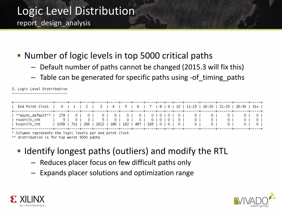
Number of logic levels in top 5000 critical paths– Default number of paths cannot be changed (2015.3 will fix this)
– Table can be generated for specific paths using -of_timing_paths
Identify longest paths (outliers) and modify the RTL– Reduces placer focus on few difficult paths only
– Expands placer solutions and optimization range
Logic Level Distributionreport_design_analysis

Identifies CDC topologies– Reports unsafe crossings and constraint issues
Structural issues reported even if exception constraints exist
Excellent cross-probing support – View schematics and exact line number in RTL
Clock Domain Crossing Reportreport_cdc
• Correct Timing Constraints
• Analyze Before Doing
• Implementation Strategies and Directives
• Congestion and Complexity
• Advanced Physical Optimization

Launch a run for every strategy– Easy To Try
– Pick the best one from design runs table
Runs Infrastructure Supports “Grid” Computing– Built-in parallel runs on different hosts (Linux)
– LSF and Sun Grid Engine
Don’t Expect This Will Solve All Your Problems
Try All The Tool OptionsSmartXplorer Style

Directive: “directs” command behavior to try alternative algorithms
– Enables wider exploration of design solutions
– Applies to opt_design, place_design, phys_opt_design, route_design
Strategy: combination of implementation commands with directives
– Performance-centric: all commands use directives for higher performance
– Congestion-centric: all commands use directives that reduce congestion
– Flow-centric: modifies the implementation flow to add steps to Defaults
power_opt_design
post-route phys_opt_design
Vivado Implementation Strategies and Directives
Faster
Compile
Higher
Performance
Quick Runtime
Optimized
Default Explore

Implementation Strategies
Strategy Name Objectives
Defaults Balance between timing closure effort and compile time
Performance_ExplorePerformance_ExplorePostRoutePhysOpt
Multiple passes of opt_design and phys_opt_design, advanced placement and routing algorithms, and post-route placement optimization. Optionally add post-route phys_opt_design.
Performance_NetDelay_* Makes delays more pessimistic for long distance and higher fanout nets with the intent to shorten their overall wirelength. Low, medium, and high settings (high = high pessimism).
Performance_WLBlockPlacement Prioritize wirelength minimization for BRAM/DSPs
Congestion_SpreadLogic_* Spread logic to aggressively avoid congested regions (low, medium, and high settings control degree of spreading)
Performance_ExploreSLLs Timing-driven optimization of SLR partitioning
Congestion_BalanceSLLsCongestion_BalanceSLRsCongestion_SpreadLogicSLLsCongestion_CompressSLR
Algorithms for alleviating congestion in SSI designs: Balance SLLs between SLRs, balance utilization in each SLR, spread logic (SSI-tailored algorithms), compress logic in SLRs to reduce SLLs
• Correct Timing Constraints
• Analyze Before Doing
• Implementation Strategies and Directives
• Congestion and Complexity
• Advanced Physical Optimization

Physical regions with– High pin density– High utilization of routing resources
Placer congestion– Congestion-aware: balances congestion vs. wirelength vs. timing slack
Cannot always eliminate congestion Cannot anticipate potential congestion introduced by hold fixing Timing estimation does not reflect detours due to congestion
– Reports congested areas seen by placer algorithms
Router congestion– Routing detours are used to handle congestion at the expense of timing– Reports largest square areas with routing utilization close to 100%
Congestion
Placer congestion tends to be more conservative than router
“Smear” Maps

Complex modules in lower hierarchy
report_design_analysis -complexity [-hierarhcial_depth N]
Complexity Report
High Rent (β), Avg fanout on larger instances
High LUT6%, MUXF* utilization
Rent’s Rule:
𝑵𝒑 = 𝑲𝒑𝑵𝒈𝜷

Placer congestion section
Note: In 2015.3 -congestion must be run in same session as place_design and route_design
Congestion Report Examplereport_design_analysis -congestion
Window defined in CLB tiles Top contributors to the region
Largest congested regionfind cells using:
get_cells -hier <Name>

Placer Congestion Report Example
Placed tile-based section (smear metrics tables)
Top contributors to the region
find using: get_cells -hier <Name>
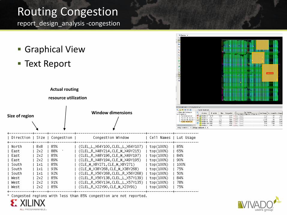
Graphical View
Text Report
Routing Congestion report_design_analysis -congestion
Actual routing
resource utilization
Window dimensionsSize of region

Reduce Logic or Pick a Bigger Device
– Look for wide bus and mux structures
Optimize modules in congested regions
– Disable LUT combining design-wide or in congested instances
Globally with synth_design -no_lc
set_property SOFT_HLUTNM “” [get_cells -hier -filter {name =~ instance/*}]
– Consider OOC synthesis with different options, strategies
– Turn off cross-boundary optimizations in synthesis
Globally with synth_design -flatten_hierarchy none
On specific modules with KEEP_HIERARCHY in RTL
Try several implementation strategies or placer directives
– Try congestion-oriented placer strategies and directives first
– Try other strategies and placer directives
=> Re-use some or all RAMB and DSP placement from good runs
Try floorplanning the congested logic
– Prevent complex modules from overlapping
– Consider dataflow through device
Potential Solutions for Congestion
• Correct Timing Constraints
• Analyze Before Doing
• Implementation Strategies and Directives
• Congestion and Complexity
• Advanced Physical Optimization
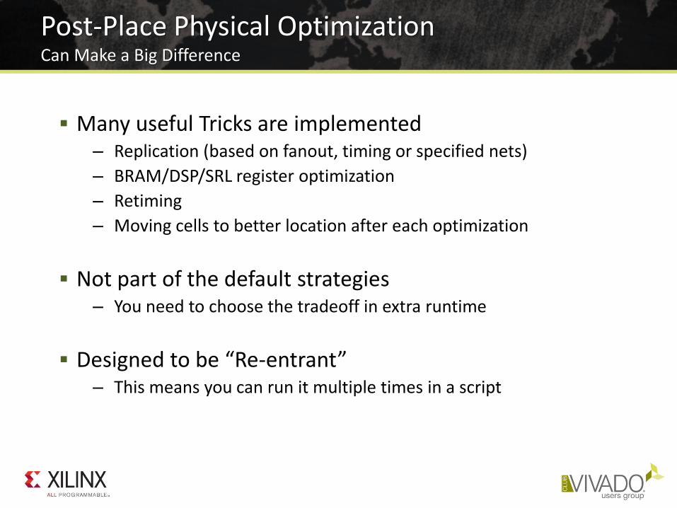
Post-Place Physical OptimizationCan Make a Big Difference
Many useful Tricks are implemented– Replication (based on fanout, timing or specified nets)
– BRAM/DSP/SRL register optimization
– Retiming
– Moving cells to better location after each optimization
Not part of the default strategies– You need to choose the tradeoff in extra runtime
Designed to be “Re-entrant”– This means you can run it multiple times in a script

Primary goal: improve WNS as much as possible– WNS limits max frequency
Secondary goal: improve TNS as much as possible– TNS increases stress on router algorithms, which
can impact WNS & WHS
Run phys_opt_design until timing is met (or close), or until WNS and TNS do not improve
Insert into run flow as a hook script
Post-Place Physical Optimization Looping
Open placed Checkpoint
phys_opt_design -directivewrite_checkpoint
WNS > 0?
route_designwrite_checkpoint
WNS > 0?
Done!
No
Yes
No
Yes

Using Post-Place Physical Optimization
DO NOT RUN post-place physical optimization if– Worst paths can only be fixed by changing the RTL
– Haven’t tried several placer directives first
– The design has not been properly baselined first
– There are CRITICAL WARNINGs that have not been dealt with
RUN post-place physical optimization if– Timing constraints are known to be good
– Worst timing violations are related to High fanout nets
Nets with loads placed far apart
High RAMB/DSP/SRL delay impact
– WNS and TNS are “reasonable” (WNS > -1ns, TNS > -10,000ns) Try several placer directives to identify the best placement startpoint

Recommended technique to over-constrain a design– XDC command: set_clock_uncertainty
– Fine granularity: clock pair
– Setup and Hold separately constrained
– Easy to reset: set_clock_uncertainty 0 <clockOptions>
– Does not affect clock relationships Modified clock periods can make CDC paths overly tight or asynchronous
Where and when to add/remove user clock uncertainty– Add before place_design or phys_opt_design (Hook Script)
Increases optimization range to provide better timing budget for router
Reduces impact of delay estimates variation or congestion
– Remove before route_design in most cases Over fixing hold is bad
Over-Constraining with Clock Uncertainty

Review Physical Optimization Timing QoR
Directive WNS TNS Failing Endpoints
Best Placement Result -0.247 -289.95 3498
Add 200ps user clock uncertainty
Popt1 (AggressiveExplore) -0.329 -866 7829
Remove 200ps user clock uncertainty
Popt2 (AggressiveExplore) -0.060 -1.971 182
Popt3 (AggressiveFanoutOpt) -0.029 -0.243 31
Routed 0.003 0.000 0
WNS and/or TNS improve after each phys_opt_design
Example (below) with partial over-constraining
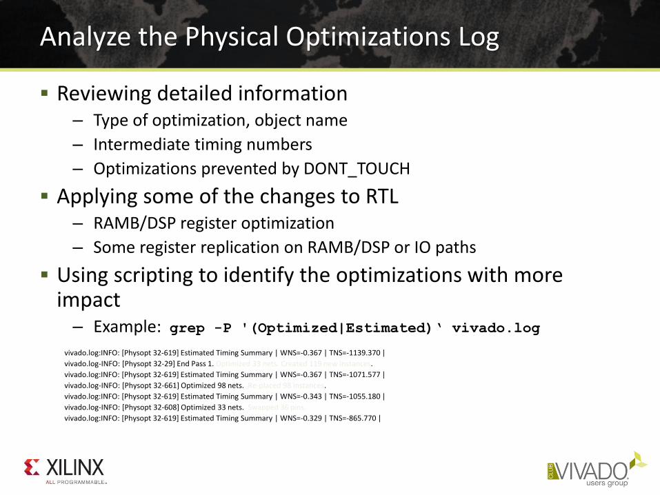
Analyze the Physical Optimizations Log
Reviewing detailed information– Type of optimization, object name
– Intermediate timing numbers
– Optimizations prevented by DONT_TOUCH
Applying some of the changes to RTL– RAMB/DSP register optimization
– Some register replication on RAMB/DSP or IO paths
Using scripting to identify the optimizations with more impact– Example: grep -P '(Optimized|Estimated)‘ vivado.log
vivado.log:INFO: [Physopt 32-619] Estimated Timing Summary | WNS=-0.367 | TNS=-1139.370 |
vivado.log-INFO: [Physopt 32-29] End Pass 1. Optimized 33 nets. Created 119 new instances.
vivado.log:INFO: [Physopt 32-619] Estimated Timing Summary | WNS=-0.367 | TNS=-1071.577 |
vivado.log-INFO: [Physopt 32-661] Optimized 98 nets. Re-placed 98 instances.
vivado.log:INFO: [Physopt 32-619] Estimated Timing Summary | WNS=-0.343 | TNS=-1055.180 |
vivado.log-INFO: [Physopt 32-608] Optimized 33 nets. Swapped 36 pins.
vivado.log:INFO: [Physopt 32-619] Estimated Timing Summary | WNS=-0.329 | TNS=-865.770 |

Post-Route Physical Optimization Expectations
When should I run post-route phys_opt_design?=> For fixing small violations only
– WNS > -0.2ns
– TNS > -10ns
How many times should I run post-route phys_opt_design?=> ONLY ONE TIME!!
– Very high runtime
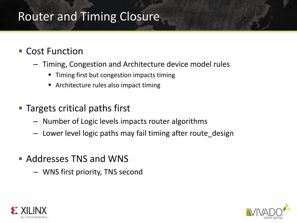
Cost Function– Timing, Congestion and Architecture device model rules
Timing first but congestion impacts timing
Architecture rules also impact timing
Targets critical paths first– Number of Logic levels impacts router algorithms
– Lower level logic paths may fail timing after route_design
Addresses TNS and WNS– WNS first priority, TNS second
Router and Timing Closure

Timing closure – A difficult problem– Start with good constraints
– Analyze and Understand issues
– Investigate RTL changes to improve timing first
Vivado has powerful analysis utilities: – Basic: report_timing, check_timing, report_exceptions, report_clock_utilization …
– Advanced: report_design_analysis, report_cdc, Baselining,
– Methodology: UltraFast Design Methodology …
Powerful optimization techniques– Phys opt looping, post-route phys opt, over constraining, floor-planning etc.
Summary


