Journal of Economic Literature 2011, 49:1, 3–71 http:www.aeaweb.org/articles.php?doi=10.1257/jel.49.1.3 3 1. Introduction T here has been a marked revival of interest in the study of the distribu- tion of top incomes using income tax data. Beginning with the research by Piketty of the long run distribution of top incomes in France (Thomas Piketty 2001, 2003), there has been a succession of studies con- structing top income share time series over the long run for more than twenty coun- tries. In using data from the income tax records, these studies use similar sources and methods as the pioneering study for the United States by Simon Kuznets (1953). Kuznets’s estimates were not, how-ever, systematically updated and, in more recent years, household survey data have become the primary source for the empirical analysis Top Incomes in the Long Run of History Anthony B. Atkinson, Thomas Piketty, and Emmanuel Saez * A recent literature has constructed top income shares time series over the long run for more than twenty countries using income tax statistics. Top incomes represent a small share of the population but a very significant share of total income and total taxes paid. Hence, aggregate economic growth per capita and Gini inequality indexes are sensitive to excluding or including top incomes. We discuss the esti- mation methods and issues that arise when constructing top income share series, including income definition and comparability over time and across countries, tax avoidance, and tax evasion. We provide a summary of the key empirical findings. Most countries experience a dramatic drop in top income shares in the first part of the twentieth century in general due to shocks to top capital incomes during the wars and depression shocks. Top income shares do not recover in the imme- diate postwar decades. However, over the last thirty years, top income shares have increased substantially in English speaking countries and in India and China but not in continental European countries or Japan. This increase is due in part to an unprecedented surge in top wage incomes. As a result, wage income comprises a larger fraction of top incomes than in the past. Finally, we discuss the theoretical and empirical models that have been proposed to account for the facts and the main questions that remain open. (JEL D31, D63, H26, N30) * Atkinson: Nullfield College, Oxford and London School of Economics. Piketty: Paris School of Economics. Saez: University of California, Berkeley. We are grateful to Facundo Alvaredo, editor Roger Gordon, Stephen Jenkins, and four anonymous referees for helpful comments and discussions.
Transcript
Journal of Economic Literature 2011, 49:1, 3–71http:www.aeaweb.org/articles.php?doi=10.1257/jel.49.1.3
3
1. Introduction
There has been a marked revival of interest in the study of the distribu-
tion of top incomes using income tax data. Beginning with the research by Piketty of
the long run distribution of top incomes in France (Thomas Piketty 2001, 2003), there has been a succession of studies con-structing top income share time series over the long run for more than twenty coun-tries. In using data from the income tax records, these studies use similar sources and methods as the pioneering study for the United States by Simon Kuznets (1953). Kuznets’s estimates were not, how-ever, systematically updated and, in more recent years, household survey data have become the primary source for the empirical analysis
Top Incomes in the Long Run of History
Anthony B. Atkinson, Thomas Piketty, and Emmanuel Saez*
A recent literature has constructed top income shares time series over the long run for more than twenty countries using income tax statistics. Top incomes represent a small share of the population but a very significant share of total income and total taxes paid. Hence, aggregate economic growth per capita and Gini inequality indexes are sensitive to excluding or including top incomes. We discuss the esti-mation methods and issues that arise when constructing top income share series, including income definition and comparability over time and across countries, tax avoidance, and tax evasion. We provide a summary of the key empirical findings. Most countries experience a dramatic drop in top income shares in the first part of the twentieth century in general due to shocks to top capital incomes during the wars and depression shocks. Top income shares do not recover in the imme-diate postwar decades. However, over the last thirty years, top income shares have increased substantially in English speaking countries and in India and China but not in continental European countries or Japan. This increase is due in part to an unprecedented surge in top wage incomes. As a result, wage income comprises a larger fraction of top incomes than in the past. Finally, we discuss the theoretical and empirical models that have been proposed to account for the facts and the main questions that remain open. (JEL D31, D63, H26, N30)
* Atkinson: Nullfield College, Oxford and London School of Economics. Piketty: Paris School of Economics. Saez: University of California, Berkeley. We are grateful to Facundo Alvaredo, editor Roger Gordon, Stephen Jenkins, and four anonymous referees for helpful comments and discussions.
Journal of Economic Literature, Vol. XLIX (March 2011)4
of inequality.1 The underlying income tax data continued to be available but remained in the shade for a long period. This relative neglect by economists adds to the interest of the findings of recent tax-based research.
The research surveyed here covers a wide variety of countries and opens the door to the comparative study of top incomes using income tax data. In contrast to existing international databases, generally restricted to the post-1970 or post-1980 period, the top income data cover a much longer period, which is important because struc-tural changes in income and wealth distri-butions often span several decades. In order to properly understand such changes, one needs to be able to put them into broader historical perspective. The new data pro-vide estimates that cover much of the twen-tieth century and in some cases go back to the nineteenth century—a length of time series familiar to economic historians but unusual for most economists. Moreover, the tax data typically allow us to decom-pose income inequality into labor income and capital income components. Economic mechanisms can be very different for the distribution of labor income (demand and supply of skills, labor market institutions, etc.) and the distribution of capital income (capital accumulation, credit constraints, inheritance law and taxation, etc.), so that it is difficult to test these mechanisms using data on total incomes.
This paper surveys the methodology, main findings, and perspectives emerg-ing from this collective research project on the dynamics of income distribution. Starting with Piketty (2001), those stud-ies have been published separately as monographs or journal articles. Recently,
1 The Kuznets series itself remained very influential in the economic history literature on U.S. inequality (see, e.g., Jeffrey G. Williamson and Peter H. Lindert 1980 and Lindert 2000).
those studies have been gathered in two edited volumes (Anthony B. Atkinson and Piketty 2007, 2010), which contain twenty-two country specific chapters along with a general summary chapter (Atkinson, Piketty, and Emmanuel Saez 2010), and a methodological chapter (Atkinson 2007b) upon which this survey draws extensively.2
We focus on the data series produced in this project on the grounds that they are fairly homogenous across countries, annual, long-run, and broken down by income source for most countries. They cover twenty-two countries, including many European countries (France, Germany, Netherlands, Switzerland, United Kingdom, Ireland, Norway, Sweden, Finland, Portugal, Spain, Italy), Northern America (United States and Canada), Australia and New Zealand, one Latin American country (Argentina), and five Asian countries (Japan, India, China, Singapore, Indonesia). They cover peri-ods that range from 15 years (China) and 30 years (Italy) to 120 years (Japan) and 132 years (Norway). Hence they offer a unique opportunity to better understand the dynamics of income and wealth distribution and the interplay between inequality and growth. The complete database is available online at the Paris School of Economics at http://g-mond.parisschoolofeconomics.eu/topincomes/.
To be sure, our series also suffer from important limitations, and we devote con-siderable space to a discussion of these. First, the series measure only top income shares and hence are silent on how inequal-ity evolves elsewhere in the distribution. Second, the series are largely concerned with gross incomes before tax. Thirdly, the defini-tion of income and the unit of observation
2 The reader is also referred to the valuable survey by Andrew Leigh (2009). Shorter summaries have also been presented in Piketty (2005, 2007), Piketty and Saez (2006), and Saez (2006).
5Atkinson, Piketty, and Saez: Top Incomes in the Long Run of History
(the individual versus the family) vary across countries making comparability of levels across countries more difficult. Even within a country, there are breaks in comparability that arise because of changes in tax legislation affecting the definition of income, although most studies try to correct for such changes to create homogenous series. Finally and perhaps most important, our series might be biased because of tax avoidance and tax evasion. Many of the studies spend consider-able time exploring in detail how tax legisla-tion changes can affect the series. The series created can therefore also be used to tackle the classical public economics issue of the response of reported income to changes in tax law.
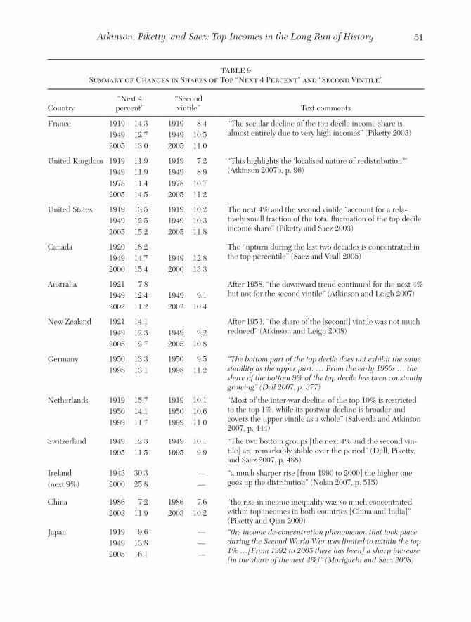
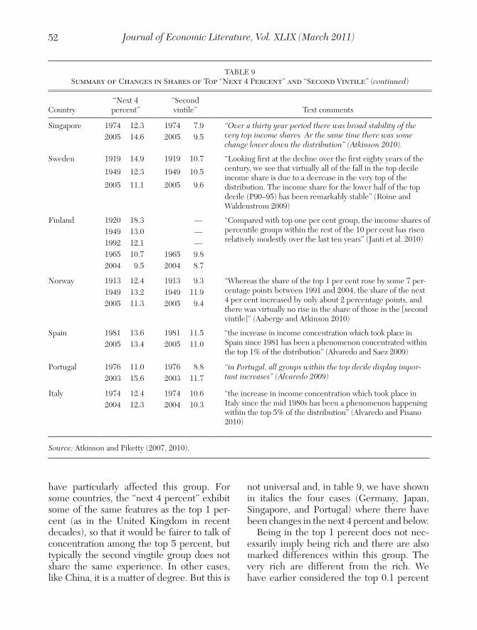
We obtain three main empirical results. First, most countries experienced a sharp drop in top income shares in the first half of the twentieth century. In these coun-tries, the fall in top income shares is often concentrated around key episodes such as the World Wars or the Great Depression. In some countries however, especially those that stayed outside World War II, the fall is more gradual during the period. In all coun-tries for which income composition data are available, in the first part of the century, top percentile incomes were overwhelmingly composed of capital income (as opposed to labor income). Therefore, the fall in the top percentile share is primarily a capital income phenomenon: top income shares fall because of a reduction in top wealth concentration. In contrast, upper income groups below the top percentile such as the next 4 percent or the second vingtile, which are comprised pri-marily of labor income, fall much less than the top percentile during the first half the twentieth century.
By 1949, the dispersion in top percen-tile income shares across the countries studied had become small. In the second half of the twentieth century, top percen-tile shares experienced a U-shape pattern,
with further declines during the immedi-ate postwar decades followed by increases in recent decades. However, the degree of the U-shape varies dramatically across coun-tries. In all of the Western English speaking countries (in Europe, North America, and Australia and New Zealand), and in China and India, there was a substantial increase in top income shares in recent decades, with the United States leading the way both in terms of timing and magnitude of the increase. Southern European countries and Nordic countries in Europe also experience an increase in top percentile shares although less in magnitude than in English speaking countries. In contrast, Continental European countries (France, Germany, Netherlands, Switzerland) and Japan experience a very flat U-shape with either no or modest increases in top income shares in recent decades.
Third, as was the case for the decline in the first half of the century, the increase in top income shares in recent decades has been quite concentrated with most of the gains accruing to the top percentile with much more modest gains (or even none at all) for the next 4 percent or the second vingtile. However, in most countries, a sig-nificant portion of the gains are due to an increase in top labor incomes, and especially wages and salaries. As a result, the fraction of labor income in the top percentile is much higher today in most countries than earlier in the twentieth century.
The rest of this paper is organized as fol-lows. In section 2, we provide motivation for the study of top incomes. In section 3, we present the methodology used to construct the database using tax statistics, and dis-cuss in details the key issues and limitations. Section 4 presents a summary of the main descriptive findings. Section 5 discusses the theoretical and empirical models that have been proposed to account for the facts while section 6 discusses how those models and explanations fit with the empirical findings.
Journal of Economic Literature, Vol. XLIX (March 2011)6
2. Motivation
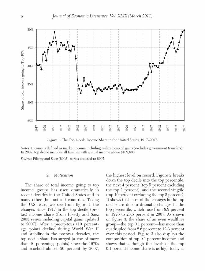
The share of total income going to top income groups has risen dramatically in recent decades in the United States and in many other (but not all) countries. Taking the U.S. case, we see from figure 1 the changes since 1917 in the top decile (pre-tax) income share (from Piketty and Saez 2003 series including capital gains updated to 2007). After a precipitous (10 percent-age point) decline during World War II and stability in the postwar decades, the top decile share has surged (a rise of more than 10 percentage points) since the 1970s and reached almost 50 percent by 2007,
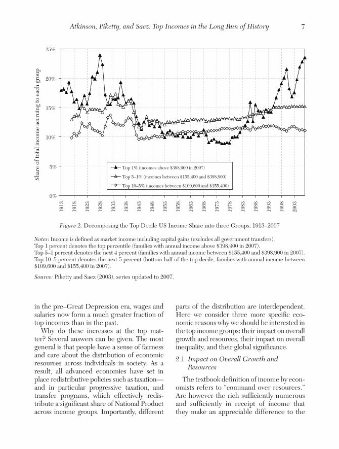
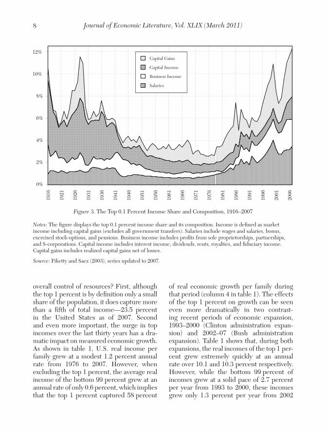
the highest level on record. Figure 2 breaks down the top decile into the top percentile, the next 4 percent (top 5 percent excluding the top 1 percent), and the second vingtile (top 10 percent excluding the top 5 percent). It shows that most of the changes in the top decile are due to dramatic changes in the top percentile, which rose from 8.9 percent in 1976 to 23.5 percent in 2007. As shown on figure 3, the share of an even wealthier group—the top 0.1 percent—has more than quadrupled from 2.6 percent to 12.3 percent over this period. Figure 3 also displays the composition of top 0.1 percent incomes and shows that, although the levels of the top 0.1 percent income share is as high today as
Figure 1. The Top Decile Income Share in the United States, 1917–2007.
Notes: Income is defined as market income including realized capital gains (excludes government transfers). In 2007, top decile includes all families with annual income above $109,600.
Source: Piketty and Saez (2003), series updated to 2007.
25%
30%
35%
40%
45%
50%
1917
1922
1927
1932
1937
1942
1947
1952
1957
1962
1967
1972
1977
1982
1987
1992
1997
2002
2007
Shar
e of
tota
l inc
ome
goin
g to
Top
10%
7Atkinson, Piketty, and Saez: Top Incomes in the Long Run of History
in the pre–Great Depression era, wages and salaries now form a much greater fraction of top incomes than in the past.
Why do these increases at the top mat-ter? Several answers can be given. The most general is that people have a sense of fairness and care about the distribution of economic resources across individuals in society. As a result, all advanced economies have set in place redistributive policies such as taxation—and in particular progressive taxation, and transfer programs, which effectively redis-tribute a significant share of National Product across income groups. Importantly, different
parts of the distribution are interdependent. Here we consider three more specific eco-nomic reasons why we should be interested in the top income groups: their impact on overall growth and resources, their impact on overall inequality, and their global significance.
2.1 Impact on Overall Growth and Resources
The textbook definition of income by econ-omists refers to “command over resources.” Are however the rich sufficiently numerous and sufficiently in receipt of income that they make an appreciable difference to the
0%
5%
10%
15%
20%
25%
1913
1918
1923
1928
1933
1938
1943
1948
1953
1958
1963
1968
1973
1978
1983
1988
1993
1998
2003
Shar
e of
tota
l inc
ome
accr
uing
to e
ach
grou
p
Top 1% (incomes above $398,900 in 2007)
Top 5–1% (incomes between $155,400 and $398,900)
Top 10–5% (incomes between $109,600 and $155,400)
Figure 2. Decomposing the Top Decile US Income Share into three Groups, 1913–2007
Notes: Income is defined as market income including capital gains (excludes all government transfers). Top 1 percent denotes the top percentile (families with annual income above $398,900 in 2007).Top 5–1 percent denotes the next 4 percent (families with annual income between $155,400 and $398,900 in 2007).Top 10–5 percent denotes the next 5 percent (bottom half of the top decile, families with annual income between $109,600 and $155,400 in 2007).
Source: Piketty and Saez (2003), series updated to 2007.
Journal of Economic Literature, Vol. XLIX (March 2011)8
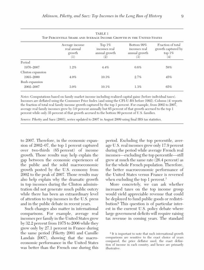
overall control of resources? First, although the top 1 percent is by definition only a small share of the population, it does capture more than a fifth of total income—23.5 percent in the United States as of 2007. Second and even more important, the surge in top incomes over the last thirty years has a dra-matic impact on measured economic growth. As shown in table 1, U.S. real income per family grew at a modest 1.2 percent annual rate from 1976 to 2007. However, when excluding the top 1 percent, the average real income of the bottom 99 percent grew at an annual rate of only 0.6 percent, which implies that the top 1 percent captured 58 percent
of real economic growth per family during that period (column 4 in table 1). The effects of the top 1 percent on growth can be seen even more dramatically in two contrast-ing recent periods of economic expansion, 1993–2000 (Clinton administration expan-sion) and 2002–07 (Bush administration expansion). Table 1 shows that, during both expansions, the real incomes of the top 1 per-cent grew extremely quickly at an annual rate over 10.1 and 10.3 percent respectively. However, while the bottom 99 percent of incomes grew at a solid pace of 2.7 percent per year from 1993 to 2000, these incomes grew only 1.3 percent per year from 2002
0%
2%
4%
6%
8%
10%
12%19
16
1921
1926
1931
1936
1941
1946
1951
1956
1961
1966
1971
1976
1981
1986
1991
1996
2001
2006
Capital Gains
Capital Income
Business Income
Salaries
Figure 3. The Top 0.1 Percent Income Share and Composition, 1916–2007
Notes: The figure displays the top 0.1 percent income share and its composition. Income is defined as market income including capital gains (excludes all government transfers). Salaries include wages and salaries, bonus, exercised stock-options, and pensions. Business income includes profits from sole proprietorships, partnerships, and S-corporations. Capital income includes interest income, dividends, rents, royalties, and fiduciary income. Capital gains includes realized capital gains net of losses.
Source: Piketty and Saez (2003), series updated to 2007.
9Atkinson, Piketty, and Saez: Top Incomes in the Long Run of History
to 2007. Therefore, in the economic expan-sion of 2002–07, the top 1 percent captured over two-thirds (65 percent) of income growth. Those results may help explain the gap between the economic experiences of the public and the solid macroeconomic growth posted by the U.S. economy from 2002 to the peak of 2007. Those results may also help explain why the dramatic growth in top incomes during the Clinton adminis-tration did not generate much public outcry while there has been an extraordinary level of attention to top incomes in the U.S. press and in the public debate in recent years.
Such changes also matter in international comparisons. For example, average real incomes per family in the United States grew by 32.2 percent from 1975 to 2006 while they grew only by 27.1 percent in France during the same period (Piketty 2001 and Camille Landais 2007), showing that the macro-economic performance in the United States was better than the French one during this
period. Excluding the top percentile, aver-age U.S. real incomes grew only 17.9 percent during the period while average French real incomes—excluding the top percentile—still grew at much the same rate (26.4 percent) as for the whole French population. Therefore, the better macroeconomic performance of the United States versus France is reversed when excluding the top 1 percent.3
More concretely, we can ask whether increased taxes on the top income group would yield appreciable revenue that could be deployed to fund public goods or redistri-bution? This question is of particular inter-est in the current U.S. policy debate where large government deficits will require raising tax revenue in coming years. The standard
3 It is important to note that such international growth comparisons are sensitive to the exact choice of years compared, the price deflator used, the exact defini-tion of income in each country, and hence are primarily illustrative.
TABLE 1Top Percentile Share and Average Income Growth in the United States
Notes: Computations based on family market income including realized capital gains (before individual taxes). Incomes are deflated using the Consumer Price Index (and using the CPI-U-RS before 1992). Column (4) reports the fraction of total real family income growth captured by the top 1 percent. For example, from 2002 to 2007, average real family incomes grew by 3.0 percent annually but 65 percent of that growth accrued to the top 1 percent while only 35 percent of that growth accrued to the bottom 99 percent of U.S. families.
Source: Piketty and Saez (2003), series updated to 2007 in August 2009 using final IRS tax statistics.
Journal of Economic Literature, Vol. XLIX (March 2011)10
response by many economists in the past has been that “the game is not worth the candle.” Indeed, net of all federal taxes, in the United States in 1976 the top percentile received only 5.8 percent of total pretax income, an amount equal to 24 percent of all federal taxes (individual, corporate, estate taxes, and social security and health contributions) in that year. However, by 2007, net of all federal taxes, the top percentile received 17.3 percent of total pretax income, or about 74 percent of all federal taxes raised in 2007.4 Therefore, it is clear that the surge in the top percentile share has greatly increased the “tax capacity” at the top of the income distribution. In budgetary terms, this cannot be ignored.5
2.2 Impact on Overall Inequality
It might be thought that top shares have little impact on overall inequality. If we draw a Lorenz curve, defined as the share of total income accruing to those below percentile p, as p goes from 0 (bottom of the distribution) to 100 (top of the distribution), then the top 1 percent would scarcely be distinguishable on the horizontal axis from the vertical endpoint, and the top 0.1 percent even less so. The most commonly used summary measure of overall inequality, the Gini coefficient, is more sensi-tive to transfers at the center of the distribu-tion than at the tails. (The Gini coefficient is defined as the ratio of the area between the Lorenz curve and the line of equality over the total area under the line of equality.)
4 The 5.8 percent and 17.3 percent figures are based on average tax rates by income groups presented in Piketty and Saez (2006). We exclude the corporate tax and the employer portion of payroll taxes as the pretax income share series are based on market income after corpo-rate taxes and employer payroll taxes. We have 5.8 per-cent = 8.8 percent * (1 − 0.262 − 0.016/2 − .068) and 17.3 percent = 23.5 percent * (1 − .225 − 0.03/2 − 0.022). The percentage of all federal taxes is obtained using total federal average tax rates that are 24.7 percent and 23.7 per-cent in 1976 and 2007 from Piketty and Saez (2006).
5 We discuss the important issue of the behavioral responses of top incomes to taxes in section 5.
But top shares can materially affect overall inequality, as may be seen from the follow-ing calculation. If we treat the very top group as infinitesimal in numbers, but with a finite share S* of total income, then, graphically, the Lorenz curve reaches 1 − S* just below p = 100. As a result, the total Gini coeffi-cient can be approximated by S* + (1 − S*) G, where G is the Gini coefficient for the population excluding the top group (Atkinson 2007b). This means that, if the Gini coefficient for the rest of the population is 40 percent, then a rise of 14 percentage points in the top share, as happened with the share of the top 1 percent in the United States from 1976 to 2006, causes a rise of 8.4 percentage points in the overall Gini. This is larger than the official Gini increase from 39.8 percent to 47.0 per-cent over the 1976–2006 period based on U.S. household income in the Current Population Survey (U.S. Census Bureau 2008, table A3).6
2.3 Top Incomes in a Global Perspective
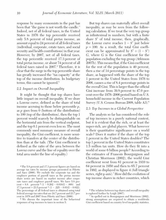
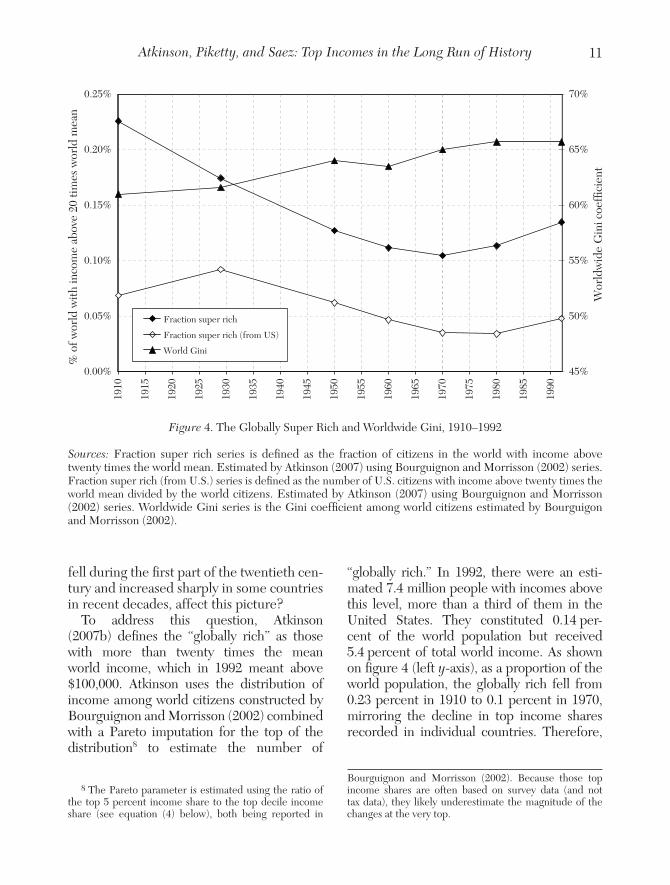
The analysis so far has considered the role of top incomes in a purely national context, but it is evident that the rich, or at least the super-rich, are global players. What however is their quantitative significance on a world scale? Does it matter if the share of the top 1 percent in the United States doubles? The top 1 percent in the United States constitutes 1.5 million tax units. How do they fit into a world of some 6 billion people? According to the estimates of Francois Bourguignon and Christian Morrisson (2002), the world Gini coefficient went from 61 percent in 1910 to 64 percent in 1950 and then to 65.7 percent in 1992, as displayed in figure 4 (full triangle series, right y-axis).7 How did the evolution of top income shares in richer countries, which
6 The relation between top shares and overall inequality is explored further by Leigh (2007).
7 As spelled out in Bourguignon and Morrisson (2002), strong assumptions are required to obtain a worldwide Gini coefficient based on country level inequality statistics.
11Atkinson, Piketty, and Saez: Top Incomes in the Long Run of History
fell during the first part of the twentieth cen-tury and increased sharply in some countries in recent decades, affect this picture?
To address this question, Atkinson (2007b) defines the “globally rich” as those with more than twenty times the mean world income, which in 1992 meant above $100,000. Atkinson uses the distribution of income among world citizens constructed by Bourguignon and Morrisson (2002) combined with a Pareto imputation for the top of the distribution8 to estimate the number of
8 The Pareto parameter is estimated using the ratio of the top 5 percent income share to the top decile income share (see equation (4) below), both being reported in
“globally rich.” In 1992, there were an esti-mated 7.4 million people with incomes above this level, more than a third of them in the United States. They constituted 0.14 per-cent of the world population but received 5.4 percent of total world income. As shown on figure 4 (left y-axis), as a proportion of the world population, the globally rich fell from 0.23 percent in 1910 to 0.1 percent in 1970, mirroring the decline in top income shares recorded in individual countries. Therefore,
Bourguignon and Morrisson (2002). Because those top income shares are often based on survey data (and not tax data), they likely underestimate the magnitude of the changes at the very top.
0.00%
0.05%
0.10%
0.15%
0.20%
0.25%
1910
1915
1920
1925
1930
1935
1940
1945
1950
1955
1960
1965
1970
1975
1980
1985
1990
% o
f wor
ld w
ith in
com
e ab
ove
20 ti
mes
wor
ld m
ean
45%
50%
55%
60%
65%
70%
Wor
ldw
ide
Gin
i coe
f�ci
ent
Fraction super rich
Fraction super rich (from US)
World Gini
Figure 4. The Globally Super Rich and Worldwide Gini, 1910–1992
Sources: Fraction super rich series is defined as the fraction of citizens in the world with income above twenty times the world mean. Estimated by Atkinson (2007) using Bourguignon and Morrisson (2002) series. Fraction super rich (from U.S.) series is defined as the number of U.S. citizens with income above twenty times the world mean divided by the world citizens. Estimated by Atkinson (2007) using Bourguignon and Morrisson (2002) series. Worldwide Gini series is the Gini coefficient among world citizens estimated by Bourguigon and Morrisson (2002).
Journal of Economic Literature, Vol. XLIX (March 2011)12
although overall inequality among world citi-zens increased, there was a compression at the top of the world distribution. But from 1970, we see a reversal and a rise in the pro-portion of globally rich above the 1950 level. The number of globally rich doubled in the United States between 1970 and 1992, which accounts for half of the worldwide increase in the number of “globally rich” and hence makes a perceptible difference to the world distribution.
2.4 Summary
There are a number of reasons for study-ing the development of top income shares. Understanding the extent of inequality at the top and the relative importance of differ-ent factors leading to increasing top shares is important in the design of public policy. Concern about the rise in top shares in a num-ber of countries has led to proposals for higher top income tax rates; other countries are con-sidering limits on remuneration and bonuses. The global distribution is coming under increasing scrutiny as globalization proceeds.
3. Methodology and Limitations
3.1 Methodology
The value of the tax data lies in the fact that, early on, the tax authorities in most countries began to compile and publish tabu-lations based on the exhaustive set of income tax returns.9 These tabulations generally report for a large number of income brackets
9 The first income tax distribution published for the United Kingdom related to 1801 (see Josiah C. Stamp 1916) but no further figures on total income are avail-able for the nineteenth century on account of the move to a schedular system. The publication of regular U.K. distributional data only commenced with the introduc-tion of supertax in 1909. Distributional data were however already by then being produced in certain parts of the British Empire. For example, in 1905, the State of Victoria (Australia) supplied a table of the distribution of income
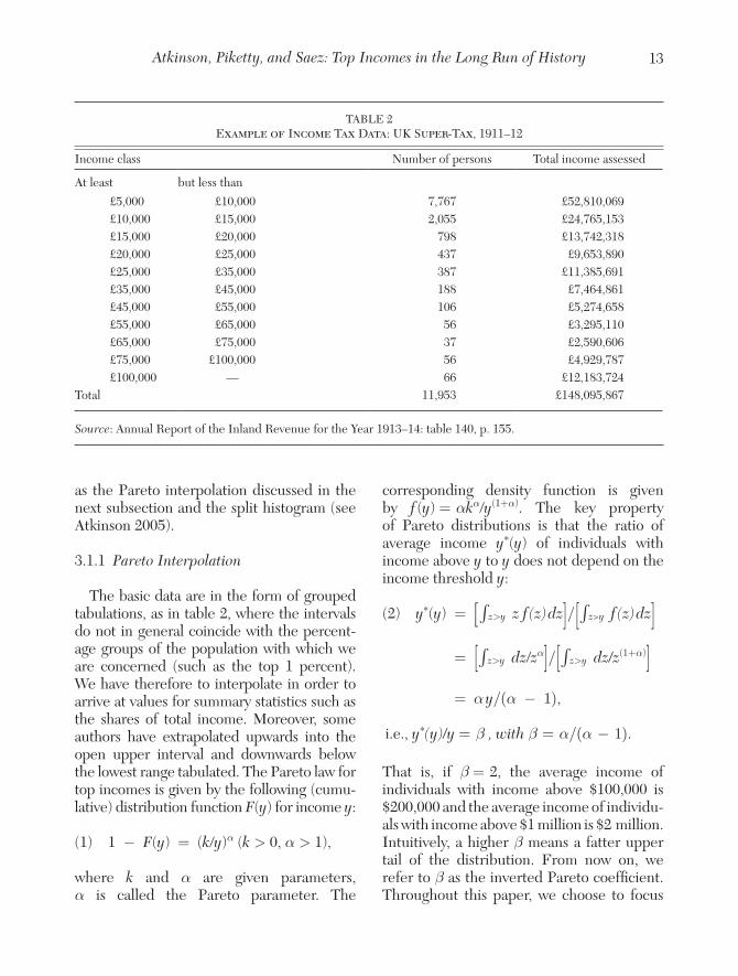
the corresponding number of taxpayers, as well as their total income and tax liability. They are usually broken down by income source: capital income, wage income, busi-ness income, etc. Table 2 shows an example of such a table from the British super-tax data for fiscal year 1911–12. These data were used by Arthur L. Bowley (1914), but it was not until the pioneering contribution of Kuznets (1953) that researchers began to combine the tax data with external estimates of the total population and the total income to estimate top income shares.10
The data in table 2 illustrate the three methodological problems addressed in this section when estimating top income shares. The first is the need to relate the number or persons to a control total to define how many tax filers represent a given fractile such as the top percentile. In the case of the United Kingdom in 1911–12, only a very small fraction of the population is subject to the super-tax: less than 12,000 taxpayers out of a total population of over twenty million tax units, i.e., not much more than 0.05 per-cent. The second issue concerns the defini-tion of income and the relation to an income control total used as the denominator in the top income share estimation. The third prob-lem is that, for much of the period, the only data available are tabulated by ranges so that interpolation estimation is required. Micro data only exist in recent decades. Note also that the tabulated data vary considerably in the number of ranges and the information provided for each range. Different meth-ods have been used for interpolation, such
in 1903 in response to a request for information from the U.K. government (House of Commons 1905, p. 233).
10 Before Kuznets, U.S. tax statistics had been used pri-marily to estimate Pareto parameters as this does not require estimating total population and total income controls (see below): see for example William L. Crum (1935), Norris O. Johnson (1935 and 1937), and Rufus S. Tucker (1938). The drawback is that Pareto parameters only capture dispersion of incomes in the top tail and—unlike top income shares—do not relate top incomes to average incomes.
13Atkinson, Piketty, and Saez: Top Incomes in the Long Run of History
as the Pareto interpolation discussed in the next subsection and the split histogram (see Atkinson 2005).
3.1.1 Pareto Interpolation
The basic data are in the form of grouped tabulations, as in table 2, where the intervals do not in general coincide with the percent-age groups of the population with which we are concerned (such as the top 1 percent). We have therefore to interpolate in order to arrive at values for summary statistics such as the shares of total income. Moreover, some authors have extrapolated upwards into the open upper interval and downwards below the lowest range tabulated. The Pareto law for top incomes is given by the following (cumu-lative) distribution function F(y) for income y:
(1) 1 − F(y) = (k/y)α (k > 0, α > 1),
where k and α are given parameters, α is called the Pareto parameter. The
corresponding density function is given by f (y) = αkα/y(1+α). The key property of Pareto distributions is that the ratio of average income y*(y) of individuals with income above y to y does not depend on the income threshold y:
(2) y*(y) = [ ∫z>y z f (z) dz]/[ ∫z>y
f (z) dz]
= [ ∫z>y d z/zα]/[ ∫z>y
d z/z(1+α)]
= α y/(α − 1),
i.e., y*(y)/y = β , with β = α/(α − 1).
That is, if β = 2, the average income of individuals with income above $100,000 is $200,000 and the average income of individu-als with income above $1 million is $2 million. Intuitively, a higher β means a fatter upper tail of the distribution. From now on, we refer to β as the inverted Pareto coefficient. Throughout this paper, we choose to focus
TABLE 2Example of Income Tax Data: UK Super-Tax, 1911–12
Income class Number of persons Total income assessed
Source: Annual Report of the Inland Revenue for the Year 1913–14: table 140, p. 155.
Journal of Economic Literature, Vol. XLIX (March 2011)14
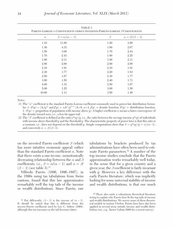
on the inverted Pareto coefficient β (which has more intuitive economic appeal) rather than the standard Pareto coefficient α. Note that there exists a one-to-one, monotonically decreasing relationship between the α and β coefficients, i.e., β = α/(α − 1) and α = β/(β − 1) (see table 3).11
Vilfredo Pareto (1896, 1896–1897), in the 1890s using tax tabulations from Swiss cantons, found that this law approximates remarkably well the top tails of the income or wealth distributions. Since Pareto, raw
11 Put differently, (β − 1) is the inverse of (α − 1). It should be noted that this is different from the inverse-Pareto coefficient used by Lee C. Soltow (1969), although this too increases as the tail becomes fatter.
tabulations by brackets produced by tax administrations have often been used to esti-mate Pareto parameters.12 A number of the top income studies conclude that the Pareto approximation works remarkably well today, in the sense that for a given country and a given year, the β coefficient is fairly invariant with y. However a key difference with the early Pareto literature, which was implicitly looking for some universal stability of income and wealth distributions, is that our much
12 There also exists a voluminous theoretical literature trying to explain why Pareto laws fit the top tails of income and wealth distributions. We survey some of these theoret-ical models in section 5 below. Pareto laws have also been applied in several areas outside income and wealth distri-bution (see, e.g., Xavier Gabaix 2009 for a recent survey).
TABLE 3Pareto-Lorenz α Coefficients versus Inverted-Pareto-Lorenz β Coefficients
Notes: (1) The “α” coefficient is the standard Pareto-Lorenz coefficient commonly used in power-law distribution formu-
las: 1−F(y) = (A/y)α and f(y) = αAα/y1+α (A>0, α>1, f(y) = density function, F(y) = distribution function, 1−F(y) = proportion of population with income above y). A higher coefficient α means a faster convergence of the density toward zero, i.e., a less fat upper tail.
(2) The “β” coefficient is defined as the ratio y*(y)/y, i.e., the ratio between the average income y*(y) of individuals with income above threshold y and the threshold y. The characteristic property of power laws is that this ratio is a constant, i.e., does not depend on the threshold y. Simple computations show that β = y*(y)/y = α/(α−1), and conversely α = β/(β−1).
15Atkinson, Piketty, and Saez: Top Incomes in the Long Run of History
larger time span and geographical scope allows us to document the fact that Pareto coefficients vary substantially over time and across countries.
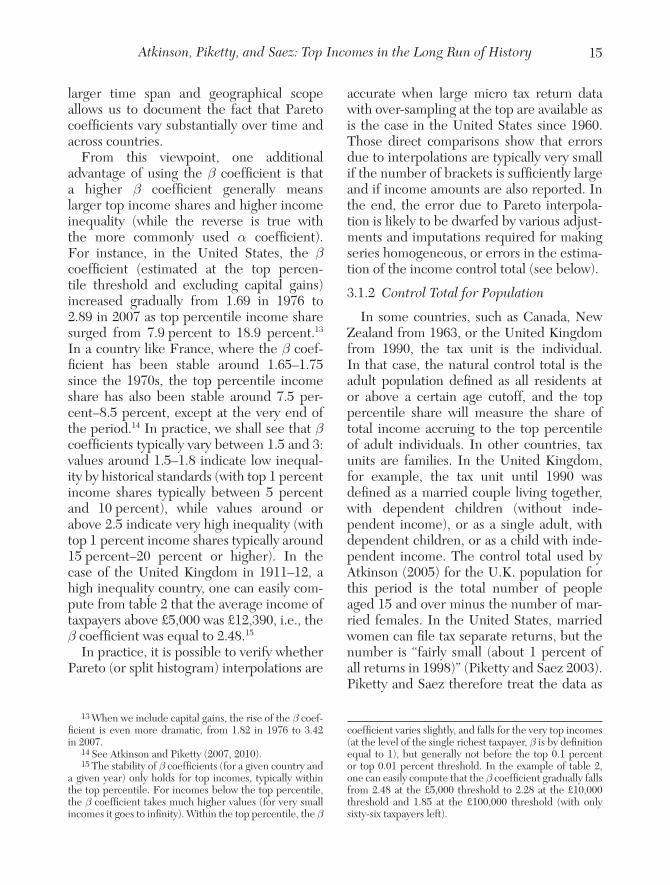
From this viewpoint, one additional advantage of using the β coefficient is that a higher β coefficient generally means larger top income shares and higher income inequality (while the reverse is true with the more commonly used α coefficient). For instance, in the United States, the β coefficient (estimated at the top percen-tile threshold and excluding capital gains) increased gradually from 1.69 in 1976 to 2.89 in 2007 as top percentile income share surged from 7.9 percent to 18.9 percent.13 In a country like France, where the β coef-ficient has been stable around 1.65–1.75 since the 1970s, the top percentile income share has also been stable around 7.5 per-cent–8.5 percent, except at the very end of the period.14 In practice, we shall see that β coefficients typically vary between 1.5 and 3: values around 1.5–1.8 indicate low inequal-ity by historical standards (with top 1 percent income shares typically between 5 percent and 10 percent), while values around or above 2.5 indicate very high inequality (with top 1 percent income shares typically around 15 percent–20 percent or higher). In the case of the United Kingdom in 1911–12, a high inequality country, one can easily com-pute from table 2 that the average income of taxpayers above £5,000 was £12,390, i.e., the β coefficient was equal to 2.48.15
In practice, it is possible to verify whether Pareto (or split histogram) interpolations are
13 When we include capital gains, the rise of the β coef-ficient is even more dramatic, from 1.82 in 1976 to 3.42 in 2007.
14 See Atkinson and Piketty (2007, 2010).15 The stability of β coefficients (for a given country and
a given year) only holds for top incomes, typically within the top percentile. For incomes below the top percentile, the β coefficient takes much higher values (for very small incomes it goes to infinity). Within the top percentile, the β
accurate when large micro tax return data with over-sampling at the top are available as is the case in the United States since 1960. Those direct comparisons show that errors due to interpolations are typically very small if the number of brackets is sufficiently large and if income amounts are also reported. In the end, the error due to Pareto interpola-tion is likely to be dwarfed by various adjust-ments and imputations required for making series homogeneous, or errors in the estima-tion of the income control total (see below).
3.1.2 Control Total for Population
In some countries, such as Canada, New Zealand from 1963, or the United Kingdom from 1990, the tax unit is the individual. In that case, the natural control total is the adult population defined as all residents at or above a certain age cutoff, and the top percentile share will measure the share of total income accruing to the top percentile of adult individuals. In other countries, tax units are families. In the United Kingdom, for example, the tax unit until 1990 was defined as a married couple living together, with dependent children (without inde-pendent income), or as a single adult, with dependent children, or as a child with inde-pendent income. The control total used by Atkinson (2005) for the U.K. population for this period is the total number of people aged 15 and over minus the number of mar-ried females. In the United States, married women can file tax separate returns, but the number is “fairly small (about 1 percent of all returns in 1998)” (Piketty and Saez 2003). Piketty and Saez therefore treat the data as
coefficient varies slightly, and falls for the very top incomes (at the level of the single richest taxpayer, β is by definition equal to 1), but generally not before the top 0.1 percent or top 0.01 percent threshold. In the example of table 2, one can easily compute that the β coefficient gradually falls from 2.48 at the £5,000 threshold to 2.28 at the £10,000 threshold and 1.85 at the £100,000 threshold (with only sixty-six taxpayers left).
Journal of Economic Literature, Vol. XLIX (March 2011)16
relating to families and take as a control total the sum of married males and all nonmarried individuals aged 20 and over.
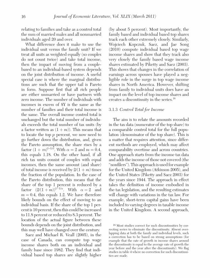
What difference does it make to use the individual unit versus the family unit? If we treat all units as weighted equally (so couples do not count twice) and take total income, then the impact of moving from a couple-based to an individual-based system depends on the joint distribution of income. A useful special case is where the marginal distribu-tions are such that the upper tail is Pareto in form. Suppose first that all rich people are either unmarried or have partners with zero income. The number of individuals with incomes in excess of $Y is the same as the number of families and their total income is the same. The overall income control total is unchanged but the total number of individu-als exceeds the total number of tax units (by a factor written as (1 + m)). This means that to locate the top p percent, we now need to go further down the distribution, and, given the Pareto assumption, the share rises by a factor (1 + m)1-1/α. With α = 2 and m = 0.4, this equals 1.18. On the other hand, if all rich tax units consist of couples with equal incomes, then the same amount (and share) of total income is received by 2/(1 + m) times the fraction of the population. In the case of the Pareto distribution, this means that the share of the top 1 percent is reduced by a factor (2/(1 + m))1−1/α. With α = 2 and m = 0.4, this equals 1.2. We have therefore likely bounds on the effect of moving to an individual basis. If the share of the top 1 per-cent is 10 percent, then this could be increased to 11.8 percent or reduced to 8.3 percent. The location of the actual figure between these bounds depends on the joint distribution, and this may well have changed over the century.
Saez and Michael R. Veall (2005), in the case of Canada, can compute top wage income shares both on an individual and family base since 1982. They find that indi-vidual based top shares are slightly higher
(by about 5 percent). Most importantly, the family based and individual based top shares track each other extremely closely. Similarly, Wojciech Kopczuk, Saez, and Jae Song (2010) compute individual based top wage income shares and show that they track also very closely the family based wage income shares estimated by Piketty and Saez (2003). This shows that changes in the correlation of earnings across spouses have played a neg-ligible role in the surge in top wage income shares in North America. However, shifting from family to individual units does have an impact on the level of top income shares and creates a discontinuity in the series.16
3.1.3 Control Total for Income
The aim is to relate the amounts recorded in the tax data (numerator of the top share) to a comparable control total for the full popu-lation (denominator of the top share). This is a matter that requires attention, since differ-ent methods are employed, which may affect comparability overtime and across countries. One approach starts from the income tax data and adds the income of those not covered (the “nonfilers”). This approach is used for example for the United Kingdom (Atkinson 2005), and the United States (Piketty and Saez 2003) for the years since 1944. The approach in effect takes the definition of income embodied in the tax legislation, and the resulting estimates will change with variations in the tax law. For example, short-term capital gains have been included to varying degrees in taxable income in the United Kingdom. A second approach,
16 Most studies correct for such discontinuities by cor-recting series to eliminate the discontinuity. Absent over-lapping data at both the family and individual levels, such a correction has to be based on strong assumptions (for example that the rate of growth in income shares around the discontinuity is equal to the average rate of growth the year before and the year after the discontinuity). We flag studies in table 4 where no correction for such discontinui-ties are made.
17Atkinson, Piketty, and Saez: Top Incomes in the Long Run of History
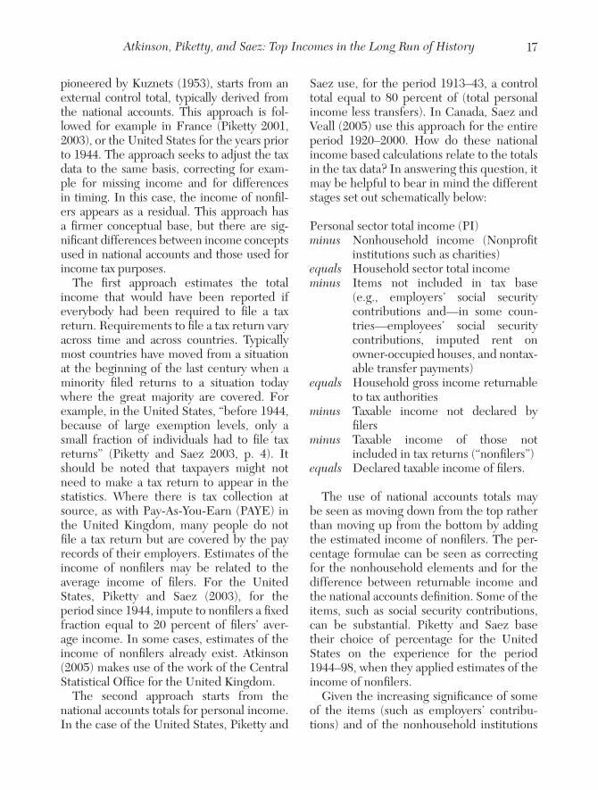
pioneered by Kuznets (1953), starts from an external control total, typically derived from the national accounts. This approach is fol-lowed for example in France (Piketty 2001, 2003), or the United States for the years prior to 1944. The approach seeks to adjust the tax data to the same basis, correcting for exam-ple for missing income and for differences in timing. In this case, the income of nonfil-ers appears as a residual. This approach has a firmer conceptual base, but there are sig-nificant differences between income concepts used in national accounts and those used for income tax purposes.
The first approach estimates the total income that would have been reported if everybody had been required to file a tax return. Requirements to file a tax return vary across time and across countries. Typically most countries have moved from a situation at the beginning of the last century when a minority filed returns to a situation today where the great majority are covered. For example, in the United States, “before 1944, because of large exemption levels, only a small fraction of individuals had to file tax returns” (Piketty and Saez 2003, p. 4). It should be noted that taxpayers might not need to make a tax return to appear in the statistics. Where there is tax collection at source, as with Pay-As-You-Earn (PAYE) in the United Kingdom, many people do not file a tax return but are covered by the pay records of their employers. Estimates of the income of nonfilers may be related to the average income of filers. For the United States, Piketty and Saez (2003), for the period since 1944, impute to nonfilers a fixed fraction equal to 20 percent of filers’ aver-age income. In some cases, estimates of the income of nonfilers already exist. Atkinson (2005) makes use of the work of the Central Statistical Office for the United Kingdom.
The second approach starts from the national accounts totals for personal income. In the case of the United States, Piketty and
Saez use, for the period 1913–43, a control total equal to 80 percent of (total personal income less transfers). In Canada, Saez and Veall (2005) use this approach for the entire period 1920–2000. How do these national income based calculations relate to the totals in the tax data? In answering this question, it may be helpful to bear in mind the different stages set out schematically below:
Personal sector total income (PI)minus Nonhousehold income (Nonprofit
institutions such as charities)equals Household sector total incomeminus Items not included in tax base
(e.g., employers’ social security contributions and—in some coun-tries—employees’ social security contributions, imputed rent on owner-occupied houses, and nontax-able transfer payments)
equals Household gross income returnable to tax authorities
minus Taxable income not declared by filers
minus Taxable income of those not included in tax returns (“nonfilers”)
equals Declared taxable income of filers.
The use of national accounts totals may be seen as moving down from the top rather than moving up from the bottom by adding the estimated income of nonfilers. The per-centage formulae can be seen as correcting for the nonhousehold elements and for the difference between returnable income and the national accounts definition. Some of the items, such as social security contributions, can be substantial. Piketty and Saez base their choice of percentage for the United States on the experience for the period 1944–98, when they applied estimates of the income of nonfilers.
Given the increasing significance of some of the items (such as employers’ contribu-tions) and of the nonhousehold institutions
Journal of Economic Literature, Vol. XLIX (March 2011)18
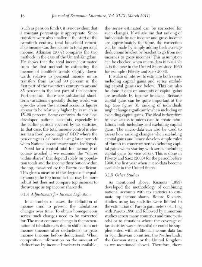
(such as pension funds), it is not evident that a constant percentage is appropriate. Since transfers were also smaller at the start of the twentieth century, total household return-able income was then closer to total personal income. Atkinson (2007) compares the two methods in the case of the United Kingdom. He shows that the total income estimated from the first method by estimating the income of nonfilers trends slightly down-wards relative to personal income minus transfers from around 90 percent in the first part of the twentieth century to around 85 percent in the last part of the century. Furthermore, there are substantial short-term variations especially during world war episodes when the national accounts figures appear to be relatively higher by as much as 15–20 percent. Some countries do not have developed national accounts, especially in the earlier periods covered by tax statistics. In that case, the total income control is cho-sen as a fixed percentage of GDP where the percentage is calibrated using later periods when National accounts are more developed.
Need for a control total for income is of course avoided if we examine the “shares within shares” that depend solely on popula-tion totals and the income distribution within the top, measured by the Pareto coefficient. This gives a measure of the degree of inequal-ity among the top incomes that may be more robust but does not compare top incomes to the average as top income shares do.
3.1.4 Adjustments for Income Definition
In a number of cases, the definition of income used to present the tabulations changes over time. To obtain homogeneous series, such changes need to be corrected for. The most common change in the presen-tation of tabulations is due to shifts from net income (income after deductions) to gross income (income before deductions). When composition information on the amount of deductions by income brackets is available,
the series estimated can be corrected for such changes. If we assume that ranking of individuals by net income and gross income are approximately the same, the correction can be made by simply adding back average deductions bracket by bracket to go from net incomes to gross incomes. This assumption can be checked when micro-data is available as is the case in the United States since 1960 for example (Piketty and Saez 2003).
It is also of interest to estimate both series including capital gains and series exclud-ing capital gains (see below). This can also be done if data on amounts of capital gains are available by income brackets. Because capital gains can be quite important at the top (see figure 3), ranking of individuals might change significantly when including or excluding capital gains. The ideal is therefore to have access to micro-data to create tabu-lations both including and excluding capital gains. The micro-data can also be used to assess how ranking changes when excluding capital gains and hence develop simple rules of thumb to construct series excluding capi-tal gains when starting with series including capital gains (or vice versa). This is done in Piketty and Saez (2003) for the period before 1960, the first year when micro-data become available in the United States.
3.1.5 Other Studies
As mentioned above, Kuznets (1953) developed the methodology of combining national accounts with tax statistics to esti-mate top income shares. Before Kuznets, studies using tax statistics were limited to the estimation of Pareto parameters (starting with Pareto 1896 and followed by numerous studies across many countries and time peri-ods) or to situations where the coverage of tax statistics was substantial or could be sup-plemented with additional income data (as in Scandinavian countries, the Netherlands, the German states, or the United Kingdom as we mentioned above). Therefore, there
19Atkinson, Piketty, and Saez: Top Incomes in the Long Run of History
exist a number of older studies in those countries computing top income shares from tax statistics. In general, those studies are limited to a few years. Those studies are sur-veyed in Lindert (2000) for the United States and the United Kingdom and Morrisson (2000) for Europe. They are also discussed in each modern study country by country. We mention the most important of those studies at the bottom of table 4. The only country for which no modern study exists and older studies exist is Denmark. Those studies for Denmark show that top incomes shares fell substantially (as in other Nordic countries) in the first half of the twentieth century till at least 1963 (Rewal Schmidt Sorensen 1993).
We also mention in table 4 other important recent country specific contributions, includ-ing those by Joachim Merz, Dierk Hirschel, and Markus Zwick (2005) and by Stefan Bach, Giacomo Corneo, and Viktor Steiner (2008) of Germany, by Bjorn Gustafsson and Birgitta Jansson (2007) of Sweden, and by Jordi Guilera Rafecas (2008) of Portugal.17
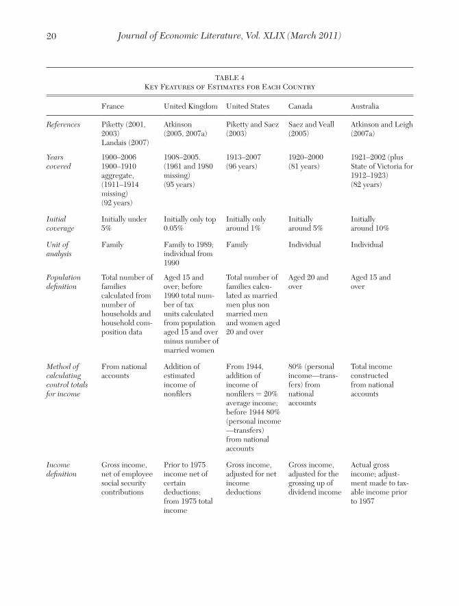
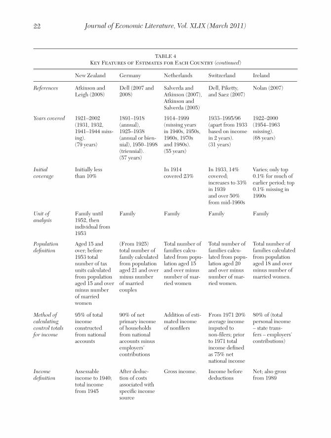
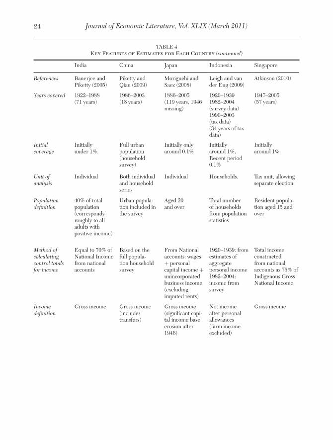
Table 4 provides a synthetic summary of the key features of the estimates for all the studies to date. It should be noted that the table refers, in some cases, to testimates updating those in the published studies.
3.2 Possible Limitations
Top income share series are constructed using tax statistics. The use of tax data is often regarded by economists with considerable disbelief. In the United Kingdom, Richard M. Titmuss wrote in 1962 a book-length critique of the income tax-based statistics on distribu-tion, concluding, “we are expecting too much from the crumbs that fall from the conven-
17 This survey does not cover the estimates for former British colonial territories being prepared as part of a proj-ect being carried out by Atkinson (apart from Singapore, shown in table 4). This project has assembled data for some forty former colonies covering the periods before and after independence. Data for French colonies and Brazil are being examined by Facundo Alvaredo.
tional tables” (p. 191). More recently, com-pilers of databases on income inequality have tended to rely on household survey data, dis-missing income tax data as unrepresentative.
These doubts are well justified for at least two reasons. The first is that tax data are collected as part of an administrative process, which is not tailored to our needs, so that the definition of income, of income unit, etc. are not neces-sarily those that we would have chosen. This causes particular difficulties for comparisons across countries, but also for time-series analy-sis where there have been substantial changes in the tax system, such as the moves to and from the joint taxation of couples. Secondly, it is obvious that those paying tax have a finan-cial incentive to present their affairs in a way that reduces tax liabilities. There is tax avoid-ance and tax evasion. The rich, in particular, have a strong incentive to understate their taxable incomes. Those with wealth take steps to ensure that the return comes in the form of asset appreciation, typically taxed at lower rates or not at all. Those with high salaries seek to ensure that part of their remuneration comes in forms, such as fringe benefits or stock options, that receive favorable tax treatment. Both groups may make use of tax havens that allow income to be moved beyond the reach of the national tax net. Third, the tax data is in general silent about the industrial compo-sition of top incomes, which limits our ability to interpret and understand changes. It would be good, for example, to know more about the links between rising top income shares and Information and Communication Technologies (ICT), but this requires other data.
These shortcomings limit what can be said from tax data but this does not mean that the data are worthless. Like all economic data, they measure with error the “true” variable in which we are interested. As with all data, there are potential sources of bias but, as in other cases, we can say something about the possible direction and magnitude of the bias. Moreover, we can compensate for some of the
Journal of Economic Literature, Vol. XLIX (March 2011)20
TABLE 4Key Features of Estimates for Each Country
France United Kingdom United States Canada Australia
Excluded Both series including and excluding capital gains presented
Excluded Included
27Atkinson, Piketty, and Saez: Top Incomes in the Long Run of History
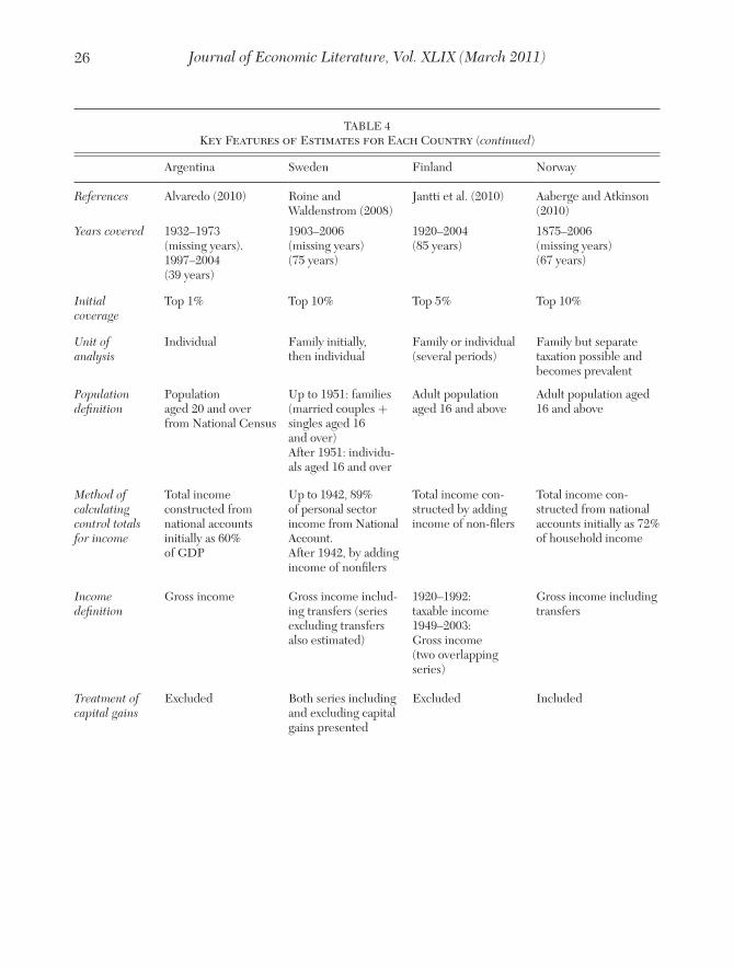
TABLE 4Key Features of Estimates for Each Country (continued)
Argentina Sweden Finland Norway
Breaks in series? Gradual shift from family to individual taxation from 1952 to 1971
Changes from family to individual taxation.Overlapping series for taxable versus gross income
Method of interpolation
Pareto Pareto Mean split histogramSurvey data (linked to tax statistics) used for 1966–2004
Mean split histogramMicro-tax data used after 1966
Special features
Comparison to household surveys provided for recent period
Top shares spike in 2005 because of dividend tax reform producing income shifting
Other References Bentzel (1952) Kraus (1981)Gustafsson and Jansson (2007)
Hjerppe and Lefgren (1974)
Journal of Economic Literature, Vol. XLIX (March 2011)28
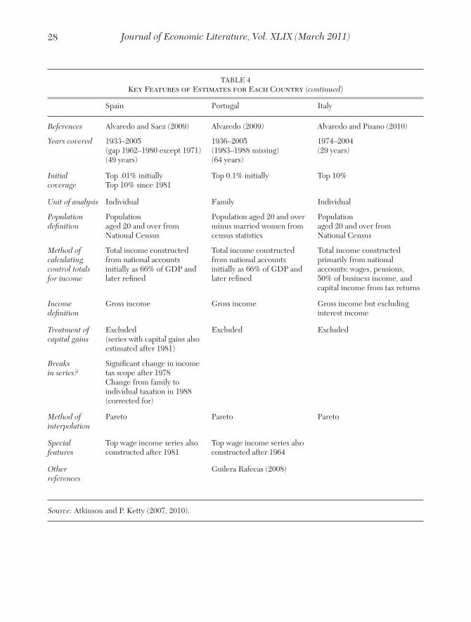
TABLE 4Key Features of Estimates for Each Country (continued)
Spain Portugal Italy
References Alvaredo and Saez (2009) Alvaredo (2009) Alvaredo and Pisano (2010)
Years covered 1933–2005 (gap 1962–1980 except 1971)(49 years)
1936–2005(1983–1988 missing)(64 years)
1974–2004(29 years)
Initial coverage
Top .01% initiallyTop 10% since 1981
Top 0.1% initially Top 10%
Unit of analysis Individual Family Individual
Population definition
Populationaged 20 and over from National Census
Population aged 20 and over minus married women from census statistics
Populationaged 20 and over from National Census
Method of calculating control totals for income
Total income constructed from national accounts initially as 66% of GDP and later refined
Total income constructed from national accounts initially as 66% of GDP and later refined
Total income constructed primarily from national accounts: wages, pensions, 50% of business income, and capital income from tax returns
Income definition
Gross income Gross income Gross income but excluding interest income
Treatment of capital gains
Excluded(series with capital gains also estimated after 1981)
Excluded Excluded
Breaks in series?
Significant change in incometax scope after 1978Change from family toindividual taxation in 1988 (corrected for)
Method of interpolation
Pareto Pareto Pareto
Special features
Top wage income series also constructed after 1981
Top wage income series also constructed after 1964
Other references
Guilera Rafecas (2008)
Source: Atkinson and P. Ketty (2007, 2010).
29Atkinson, Piketty, and Saez: Top Incomes in the Long Run of History
shortcomings of the income tax data. It is true that income tax data cover only the taxpaying population, which, in the early years of income tax, was typically only a small fraction of the total population. As a result, tax data cannot be used to describe the whole distribution but we can estimate the upper part of the Lorenz curve, i.e., top income shares.
But why not use household surveys that cover the whole (noninstitutional) popula-tion? Why use income tax data? There are two main answers. The first is that household sur-veys themselves are not without shortcom ings. These include sampling error, which may be sizable with the typical sample sizes for sur - veys, whereas tax data drawn from administra- tive records are based on very much larger samples. Indeed, in some cases the tax statis-tics relate to the whole universe of taxpayers. Household surveys suffer from differential nonresponse and incomplete response (these two being the survey counterpart of tax eva-sion), as well as measurement error, Such problems particularly affect the top income ranges, as is recognized in studies that com-bine household survey data with information on upper income ranges from tax sources (see, for example, in the United Kingdom, Michael Brewer et al. 2008). Indeed, most surveys impose top coding to limit the effects of mea- surement error on aggregates, which severely limit the analysis of top incomes using survey data. The second answer is that household sur- veys are a fairly recent innovation. Household surveys only became regular in most coun-tries in the 1970s or later and, in a number of cases, they are held at intervals rather than annually. The beauty of income tax evidence is that it is available for long runs of years, typically on an annual basis, and that it is available for a wide variety of countries.
3.2.1 Comparison with Household Survey Data: U.S. Case Study
The important recent study by Richard V. Burkhauser et al. (2009) tries to reconcile
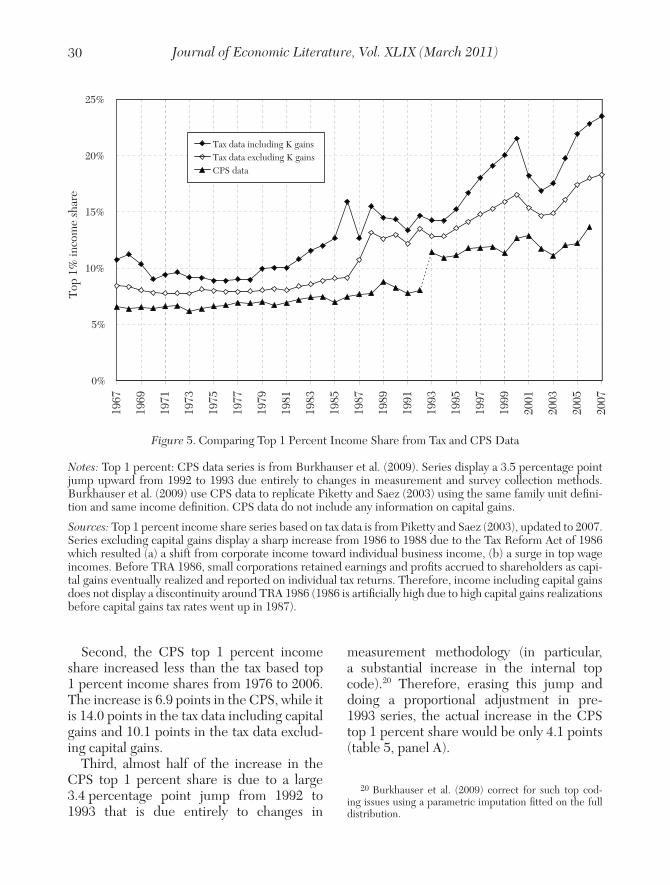
the Piketty and Saez (2003) top income share series, estimated with tax statistics, with top income shares measured using CPS data but following the same methodology as in Piketty and Saez (2003) in terms of income definition and family unit.18 Burkhauser et al. (2009) find that their CPS based top income share series match the Piketty and Saez (2003) series very closely for the second vingtile and the next 4 percent (i.e., the top decile excluding the top percentile). As depicted on figure 5, the top 1 percent share measured by the CPS also appears to follow the same qualitative trend as the top 1 percent share from tax data. However there are important quantitative differences that remain, espe-cially comparing the CPS series with the tax series including realized capital gains (which are not measured in the CPS questionnaire). Four points are worth noting.
First, the top 1 percent share measured by the CPS is consistently lower than the top 1 percent income share measured with tax data. This is due to the fact that (a) the CPS does not record important income sources at the top (such as realized capital gains or stock option gains), (b) CPS incomes are by design recorded with top code,19 (c) there might be underreporting of incomes at the top in the CPS (i.e., some top income individuals might decide to under report their true income, even in the absence of uncertainty about the income concept).
18 Edward N. Wolff and Ajit Zacharias (2009) and Arthur B. Kennickell (2009) also compute top income shares using the Survey of Consumer Finances, which is not top coded and oversamples the rich. Wolff and Zacharias (2009) in particular use wealth data to estimate more comprehensive measures of capital income that cannot be observed in tax data. The trend of their estimated series is in line with the tax based estimates of Piketty and Saez (2003).
19 Burkhauser et al. (2009) use the internal CPS. The internal CPS is further top coded for confidentiality rea-sons before being publicly disclosed. However, even the internal CPS remains top coded by design. Such top codes are necessary in survey data to avoid having a handful of reporting errors having significant effects on aggregate statistics.
Journal of Economic Literature, Vol. XLIX (March 2011)30
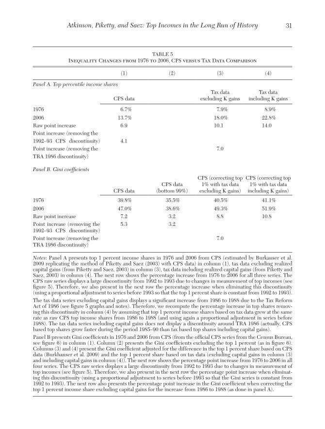
Second, the CPS top 1 percent income share increased less than the tax based top 1 percent income shares from 1976 to 2006. The increase is 6.9 points in the CPS, while it is 14.0 points in the tax data including capital gains and 10.1 points in the tax data exclud-ing capital gains.
Third, almost half of the increase in the CPS top 1 percent share is due to a large 3.4 percentage point jump from 1992 to 1993 that is due entirely to changes in
measurement methodology (in particular, a substantial increase in the internal top code).20 Therefore, erasing this jump and doing a proportional adjustment in pre-1993 series, the actual increase in the CPS top 1 percent share would be only 4.1 points (table 5, panel A).
20 Burkhauser et al. (2009) correct for such top cod-ing issues using a parametric imputation fitted on the full distribution.
0%
5%
10%
15%
20%
25%
1967
1969
1971
1973
1975
1977
1979
1981
1983
1985
1987
1989
1991
1993
1995
1997
1999
2001
2003
2005
2007
Top
1%
inco
me
shar
e
Tax data including K gainsTax data excluding K gainsCPS data
Figure 5. Comparing Top 1 Percent Income Share from Tax and CPS Data
Notes: Top 1 percent: CPS data series is from Burkhauser et al. (2009). Series display a 3.5 percentage point jump upward from 1992 to 1993 due entirely to changes in measurement and survey collection methods. Burkhauser et al. (2009) use CPS data to replicate Piketty and Saez (2003) using the same family unit defini-tion and same income definition. CPS data do not include any information on capital gains.
Sources: Top 1 percent income share series based on tax data is from Piketty and Saez (2003), updated to 2007. Series excluding capital gains display a sharp increase from 1986 to 1988 due to the Tax Reform Act of 1986 which resulted (a) a shift from corporate income toward individual business income, (b) a surge in top wage incomes. Before TRA 1986, small corporations retained earnings and profits accrued to shareholders as capi-tal gains eventually realized and reported on individual tax returns. Therefore, income including capital gains does not display a discontinuity around TRA 1986 (1986 is artificially high due to high capital gains realizations before capital gains tax rates went up in 1987).
31Atkinson, Piketty, and Saez: Top Incomes in the Long Run of History
TABLE 5Inequality Changes from 1976 to 2006, CPS versus Tax Data Comparison
(1) (2) (3) (4)
Panel A. Top percentile income shares
CPS dataTax data
excluding K gainsTax data
including K gains
1976 6.7% 7.9% 8.9%
2006 13.7% 18.0% 22.8%Raw point increase 6.9 10.1 14.0Point increase (removing the 1992–93 CPS discontinuity) 4.1Point increase (removing the 7.0TRA 1986 discontinuity)
Panel B. Gini coefficients
CPS dataCPS data
(bottom 99%)
CPS (correcting top 1% with tax data
excluding K gains)
CPS (correcting top 1% with tax data
including K gains)
1976 39.8% 35.5% 40.5% 41.1%
2006 47.0% 38.6% 49.3% 51.9%Raw point increase 7.2 3.2 8.8 10.8Point increase (removing the 1992–93 CPS discontinuity)
5.3 3.2
Point increase (removing the TRA 1986 discontinuity)
7.0
Notes: Panel A presents top 1 percent income shares in 1976 and 2006 from CPS (estimated by Burkauser et al. 2009 replicating the method of Piketty and Saez (2003) with CPS data) in column (1), tax data excluding realized capital gains (from Piketty and Saez, 2003) in column (3), tax data including realized capital gains (from Piketty and Saez, 2003) in column (4). The next row shows the percentage increase from 1976 to 2006 for all three series. The CPS raw series displays a large discontinuity from 1992 to 1993 due to changes in measurement of top incomes (see figure 5). Therefore, we also present in the next row the percentage increase when eliminating this discontinuity (using a proportional adjustment to series before 1993 so that the top 1 percent share is constant from 1992 to 1993).The tax data series excluding capital gains displays a significant increase from 1986 to 1988 due to the Tax Reform Act of 1986 (see figure 5 graphs and notes). Therefore, we recompute the percentage increase in top shares remov-ing this discontinuity in column (4) by assuming that top 1 percent income shares based on tax data grew at the same rate as raw CPS top income shares from 1986 to 1988 (and using again a proportional adjustment in series before 1988). The tax data series including capital gains does not display a discontinuity around TRA 1986 (actually, CPS based top shares grow faster during the period 1985–90 than tax based top shares including capital gains).Panel B presents Gini coefficients in 1976 and 2006 from CPS (from the official CPS series from the Census Bureau, see figure 6) in column (1). Column (2) presents the Gini coefficients excluding the top 1 percent (as in figure 6). Columns (3) and (4) present the Gini coefficient adjusted for the difference in the top 1 percent share based on CPS data (Burkhauser et al. 2009) and the top 1 percent share based on tax data (excluding capital gains in column (3) and including capital gains in column (4)). The next row shows the percentage point increase from 1976 to 2006 in all four series. The CPS raw series displays a large discontinuity from 1992 to 1993 due to changes in measurement of top incomes (see figure 5). Therefore, we also present in the next row the percentage point increase when eliminat-ing this discontinuity (using a proportional adjustment to series before 1993 so that the Gini series is constant from 1992 to 1993). The next row also presents the percentage point increase in the Gini coefficient when correcting the top 1 percent income share excluding capital gains for the increase from 1986 to 1988 (as done in panel A).
Journal of Economic Literature, Vol. XLIX (March 2011)32
Fourth, there is a concern that tax based top income shares also exaggerate the increase because of income shifting toward the individual tax base following the tax rate reductions on the 1980s. Indeed, the series excluding capital gains does display a large 4.0 point upward jump from 1986 to 1988. As is well known (Daniel R. Feenberg and James M. Poterba 1993, Saez 2004), almost one-half of this jump is due to a shift from corporate income toward individual business income due to the Tax Reform Act of 1986.21 However, corporate retained earnings trans-late into capital gains that are eventually real-ized and reported on individual tax returns. Therefore, in the medium run, this shift will be matched by an equivalent reduction in capital gains. Indeed, the top 1 percent income share series including capital gains display no notable discontinuity around the TRA 1986 episode (the CPS top income shares increase as fast as the tax return based top income share including capital gains in the medium run from 1985 to 1990).22
Therefore, from 1976 to 2006 and eras-ing the 1992–93 measurement discontinu-ity in the CPS, the CPS top 1 percent share effectively misses 10.4 points of the surge of the top 1 percent income share relative to income tax data including realized capi-tal gains (the most economically meaningful series to capture total real top incomes). As we show on figure 6 and table 5 (panel B), this has a substantial impact on the official
21 TRA 1986 made it more advantageous for closely held businesses to shift from corporate to pass-through entities taxed solely at the individual level. Furthermore, those firms that remain corporate have an incentive to shift more of their taxable income to the personal tax base. This can be done in many ways, e.g., higher royalty payments, payments for rent, higher interest payments, as well as higher wage payments to entrepreneurs (Roger H. Gordon and Joel B. Slemrod 2000).
22 The top income share including capital gains is abnormally high in 1986 because of very large capital gain realizations in that year to avoid the higher capital gain tax rates after TRA 1986, a well established finding clearly vis-ible on figure 3.
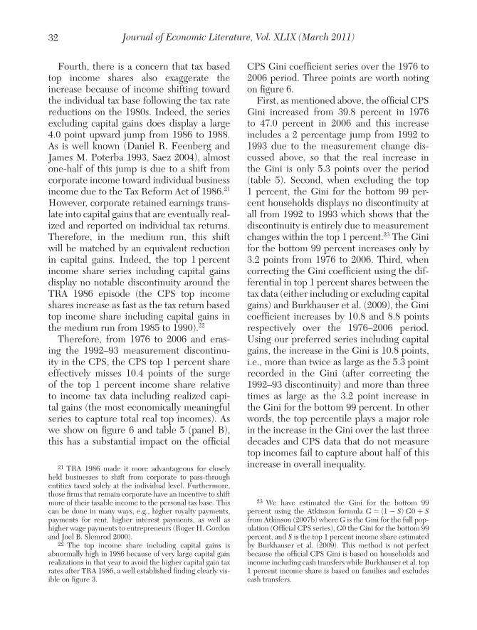
CPS Gini coefficient series over the 1976 to 2006 period. Three points are worth noting on figure 6.
First, as mentioned above, the official CPS Gini increased from 39.8 percent in 1976 to 47.0 percent in 2006 and this increase includes a 2 percentage jump from 1992 to 1993 due to the measurement change dis-cussed above, so that the real increase in the Gini is only 5.3 points over the period (table 5). Second, when excluding the top 1 percent, the Gini for the bottom 99 per-cent households displays no discontinuity at all from 1992 to 1993 which shows that the discontinuity is entirely due to measurement changes within the top 1 percent.23 The Gini for the bottom 99 percent increases only by 3.2 points from 1976 to 2006. Third, when correcting the Gini coefficient using the dif-ferential in top 1 percent shares between the tax data (either including or excluding capital gains) and Burkhauser et al. (2009), the Gini coefficient increases by 10.8 and 8.8 points respectively over the 1976–2006 period. Using our preferred series including capital gains, the increase in the Gini is 10.8 points, i.e., more than twice as large as the 5.3 point recorded in the Gini (after correcting the 1992–93 discontinuity) and more than three times as large as the 3.2 point increase in the Gini for the bottom 99 percent. In other words, the top percentile plays a major role in the increase in the Gini over the last three decades and CPS data that do not measure top incomes fail to capture about half of this increase in overall inequality.
23 We have estimated the Gini for the bottom 99 percent using the Atkinson formula G = (1 − S) G0 + S from Atkinson (2007b) where G is the Gini for the full pop-ulation (Official CPS series), G0 the Gini for the bottom 99 percent, and S is the top 1 percent income share estimated by Burkhauser et al. (2009). This method is not perfect because the official CPS Gini is based on households and income including cash transfers while Burkhauser et al. top 1 percent income share is based on families and excludes cash transfers.
33Atkinson, Piketty, and Saez: Top Incomes in the Long Run of History
30%
35%
40%
45%
50%
55%19
67
1969
1971
1973
1975
1977
1979
1981
1983
1985
1987
1989
1991
1993
1995
1997
1999
2001
2003
2005
2007
Gin
i coe
f�ci
ent
Adjusted with tax data including K gains
Adjusted with tax data excluding K gains
Of�cial CPS series
CPS data (bottom 99%)
Figure 6. CPS Gini Coefficients: Correcting Top 1 Percent with Tax Data
Notes: Official CPS data series is the official Gini coefficient estimated from CPS data by the Bureau of Census (Current Population Reports, Series P60–231). The unit of analysis is the household (not the family) and income includes cash transfers. The discontinuity from 1992 to 1993 is due to changes in measurement and survey collec-tion methods.
CPS data (bottom 99 percent) series report the Gini coefficient based on CPS data but excluding the top 1 percent. We have computed those series using the formula G = (1 − S)G0 + S from Atkinson (2007b) where G is the Gini for the full population (Official CPS series), G0 the Gini for the bottom 99 percent, and S is the top 1 percent income share (from Burkhauser et al. 2009, depicted on figure 5). Note that the discontinuity from 1992 to 1993 vanishes entirely for the bottom 99 percent Gini demonstrating that the discontinuity in the Gini is entirely due to changes in the measurement and censoring of top incomes within the top 1 percent.
Adjusted tax data series adjusts the CPS Gini coefficient for the rise in the top percentile share in the tax data not captured by the CPS. Defining as D the difference in the top percentile shares from tax data (from Piketty and Saez, 2003) and the CPS data (from Burkhauser et al. 2009), the adjusted Gini is computed as (1 − D) G + D where G is the Official CPS Gini series (displayed in the graph). We have made those corrections both using the tax data series including capital gains and using tax data series excluding capital gains. Again, the fact that the discontinuity from 1992 to 1993 disappears in those corrected series confirms that the discontinuity in the official CPS Gini series is entirely due to changes in the measurement of top incomes within the top 1 percent.
The Gini correction using series including capital gains is the most meaningful economically because (a) realized capital gains are a significant source of income at the top (as many corporations retain substantial earnings or dis-tribute profits using share repurchases instead of dividends), (b) top 1 percent income share series including capital gains are not affected as much by tax manipulation around TRA 1986 (as explained in the notes to figure 5).
Journal of Economic Literature, Vol. XLIX (March 2011)34
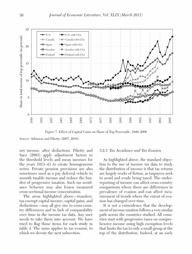
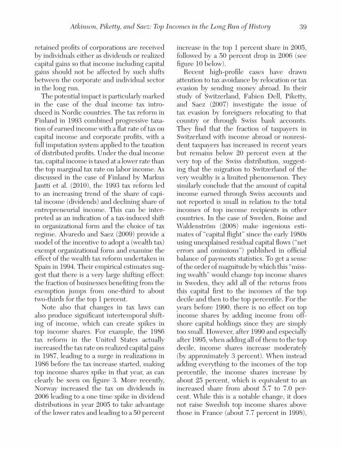
3.2.2 The Definition of Income
Taxes affect the substance of the income distribution, and we return to this in sec-tion 4, but they also affect the form of the income distribution statistics. In all cases, the estimates follow the tax law, rather than a “preferred” definition of income, such as the Haig–Simons comprehensive definition, which includes such items as imputed rent, fringe employment benefits, or accruing cap-ital gains and losses. In principle, transfers from the government should not be included in pre-fisc incomes as they are part of the government redistributive schemes which tax pre-fisc incomes and provide transfers. In practice, the largest cash transfer pay-ments are public pensions which are often related to social security contributions dur-ing the work life and hence can be consid-ered as deferred earnings. Means-tested transfer programs are, in general, nontaxable and excluded from the estimates presented. Estimating top post-fisc income shares based on incomes after taxes and transfers is also of great interest to measure the direct redis-tributive effects of taxes and transfer poli-cies.24 Some studies, such as Atkinson (2005) for the United Kingdom, Piketty (2001) for France, and Piketty and Saez (2007) for the United States since 1960, have also esti-mated post-fisc top income shares.
For a single country study, it may be rea-sonable to assume that income is a concept well understood in that context. Alternatively, one may assume that all taxable incomes dif-fer from the preferred definition by the same percentage. Neither of these assumptions, however, seems particularly satisfactory and use of taxable income may well affect the
24 Taxes and transfers might also have indirect redistrib-utive effects through behavioral responses. For example, high income earners might work less and hence earn less if taxes increase. We come back to this important point in section 5.
conclusions drawn about changes over time. When we come to a cross-country com-parison, there seems an even stronger case for adopting a definition of income that is common across countries and that does not depend on the specificities of the tax law in each country. Approaching a common defini-tion of income does however pose consider-able problems, as illustrated by the treatment of transfers (which have grown very con-siderably in importance over the century), by capital gains, by the interrelation with the corporate tax system, and by tax deduc-tions. The studies for the United States and Canada subtract social security transfers on the grounds that they are either partially or totally exempt from tax. In other countries, such as Australia, New Zealand, Norway, and the United Kingdom, the tax treatment of transfers differs, with typically more transfers being brought into taxation over time.
Perhaps the most important aspect that affects the comparability of series over time within each country has been the ero-sion of capital income from the progressive income tax base. Early progressive income tax systems included a much larger fraction of capital income than most present pro gressive income tax systems. Indeed, over time, many sources of capital income, such as interest income or returns on pension funds, have been either taxed separately at flat rates or fully exempted and, hence, have disappeared from the tax base. Some early income tax sys-tems (such as France from 1914 to 1964) also included imputed rents of homeowners in the tax base, but today imputed rents are typically excluded. As a result of this imputed rent exclu-sion and the development of numerous other forms of legally tax-exempt capital income, the share of capital income that is reportable on income tax returns, and hence included in the series presented, has significantly decreased over time. To the extent that such excluded capital income accrues dispropor-tionately to top income groups, this will lead
35Atkinson, Piketty, and Saez: Top Incomes in the Long Run of History
to an underestimation of top income shares. Ideally, one would want to impute excluded capital income back to each income group. Because of lack of data, such an imputation is very difficult to fully carry out.25 Some of the studies discuss whether the exclusion of capital income affects the series. For exam-ple, Chiaki Moriguchi and Saez (2008), in the case of Japan, use survey data to estimate how interest income—today almost completely excluded from the comprehensive income tax base in Japan—is distributed across income groups. In the case of France, Piketty (2001, 2003) has shown that the long-run decline of top income shares was robust in the sense that even an upper bound imputation of today’s tax-exempt capital incomes to today’s reported top incomes would be largely insufficient to undo the observed fall. In the estimates of top shares for Norway (Rolf Aaberge and Atkinson 2010), a calculation has been made of income including the “full” return to stocks, but no systematic attempt has been made to impute full capital income on a comparable basis over time and across countries. We view this as one of the main shortcomings—prob-ably the main shortcoming—of our data set. As we shall see in sections below, this limits the extent to which one can use our data set to rigorously test the theoretical economic mechanisms at play.
The treatment of capital gains and losses also differs across time and across countries. For a number of countries, series both includ-ing and excluding capital gains have been produced (see table 4). As shown in figure 7, the effects of the inclusion of capital gains on the share of the top percentile is often substantial. In the case of Sweden, Jesper Roine and Daniel Waldenström (2008) note that “over the past two decades the general picture turns out to depend crucially on
25 Wolff and Zacharias (2009) use the Survey of Consumer Finance and combine income and wealth data to estimate broader measures of capital income since 1982.
how income from capital gains is treated. If we include capital gains, Swedish income inequality has increased quite substantially; when excluding them, top income shares have increased much less.” In all cases, only realized capital gains are included, if at all, in tax statistics and no information on accru-ing capital gains is available. Some accrued capital gains are never realized, for example, when there are step-up of basis provisions at time of death as in the United States.26
Finally, although the distinction between capital and labor income is clear conceptu-ally, it is often partly blurred in the compo-sitional tax statistics. For example, realized capital gains of business owners often cor-respond to the sale of accumulated earnings of entrepreneurs in their firm, rather than return on capital. Stock-option compensa-tion sometimes appears as wage income but sometimes as capital income in tax statistics depending on the tax law.
Income tax systems differ in the extent of their provisions allowing the deduction of such items as interest paid, depreciation, pension contributions, alimony payments, and charitable contributions. Income from which these deductions have been subtracted is often referred to as “net income.” (We are not referring here to personal exemptions.) The aim is in general to measure gross income before deductions, but this is not always possible. The French estimates show income after deducting employee social security contributions. In a number of coun-tries, the earlier income tax distributions refer to income after these deductions, but the later distributions refer to gross income. In the United States, the income tax returns prior to 1944 showed the distribution by
26 Using the Survey of Consumer Finances, Poterba and Scott Weisbenner (2001) estimate that, in 1998, capital gains unrealized at time of death were $42.8bn (table 10-8, p. 440), i.e., slightly less than 10 percent of the $440bn of net realized capital gains reported on individual tax returns in 1998 (Piketty and Saez 2003).
Journal of Economic Literature, Vol. XLIX (March 2011)36
net income, after deductions. Piketty and Saez (2003) apply adjustment factors to the threshold levels and mean incomes for the years 1913–43 to create homogeneous series. Private pension provisions are also sometimes used as a pay deferral vehicle to smooth taxable income and reduce the bur-den of progressive taxation. Such tax avoid-ance behavior may also lessen measured cross-sectional income concentration.
The areas highlighted above—transfers, tax-exempt capital income, capital gains, and deductions—may all give rise to cross-coun-try differences and to lack of comparability over time in the income tax data. Any user needs to take them into account. We have tried to flag those items for each study in table 4. The same applies to tax evasion, to which we devote the next subsection.
3.2.3 Tax Avoidance and Tax Evasion
As highlighted above, the standard objec-tion to the use of income tax data to study the distribution of income is that tax returns are largely works of fiction, as taxpayers seek to avoid and evade being taxed. The under-reporting of income can affect cross-country comparisons where there are differences in prevalence of evasion and can affect mea-surement of trends where the extent of eva-sion has changed over time.
It is not a coincidence that the develop-ment of income taxation follows a very similar path across the countries studied. All coun-tries start with progressive taxes on compre-hensive income using high exemption levels that limits the tax to only a small group at the top of the distribution. Indeed, at an early
0
5
10
15
20
2519
49
1953
1957
1961
1965
1969
1973
1977
1981
1985
1989
1993
1997
2001
2005
Shar
e in
tota
l inc
ome
of to
p pe
rcen
tile
(in p
erce
nt) U.S. U.S. with CGs
Canada Canada with CGs
Spain Spain with CGs
Sweden Sweden with CGs
Finland Finland with CGs
Figure 7. Effect of Capital Gains on Share of Top Percentile, 1949–2006
Source: Atkinson and Piketty (2007, 2010).
37Atkinson, Piketty, and Saez: Top Incomes in the Long Run of History
stage of industrial development, when a sub-stantial fraction of economic activity takes place in small informal businesses, it is just not possible for the government to enforce a comprehensive income tax on a wide share of the population.27 However, even in early stages of economic development, Alvaredo and Saez (2009) note “the incomes of high income individuals are identifiable because they derive their incomes from large and modern businesses or financial institutions with verifiable accounts, or from highly paid (and verifiable) salaried positions, or prop-erty income from publicly known assets (such as large land estates with regular rental income).”28 Therefore, it is conceivable that the early progressive income taxes, upon which statistics those studies are based, cap-tured reasonably well most components of top incomes. If tax avoidance and evasion has increased since then, the degree of equaliza-tion may be overstated.
Williamson and Lindert (1980) confront the issue directly for the data for the United States. They ask whether “superior tax avoid-ance” can have accounted for the income leveling over the period 1929–51 found by Kuznets (1953). As they note, the argument of spurious leveling depends on a double differential: that tax avoidance/evasion has increased, and that it has increased faster for the top incomes. On the basis of compari-sons of reported income totals with national accounts data, they conclude that “even under a strong assumption about changes in the pattern of lying, most of the leveling remains unobscured” (1980, p. 88).
27 Even today in the most advanced economies, small informal businesses may escape the individual income taxes.
28 Indeed, before comprehensive taxation starts, most countries had already adopted schedular separate taxes on specific income sources such as wages and salaries, profits from large businesses, rental income from large estates. Such schedular taxes emerge when economic development makes enforcement feasible.
The extent of contemporary tax evasion is considered specifically in a number of studies. In the case of Sweden, Roine and Waldenström (2008) conclude that over-all evasion is modest (around 5 percent of all incomes) and that there is no reason to believe that underreporting has changed dramatically over time. A speculative reason for this may be that while the incentives to underreport have increased as tax rates have gone up over time the administrative control over tax compliance has also been improved. The Nordic countries may well be differ-ent. In the case of Italy, Alvaredo and Elena Pisano (2010) note the widespread view of tax evasion being much higher than in other OECD countries. Audits and subsequent scandals involving show-business people, well-known fashion designers, and sport stars help support this idea among the gen-eral public, even when they also provide evi-dence about the fact that top income earners are very visible for the tax administration. The evidence for Italy does indeed suggest that evasion is important among small busi-nesses and the self-employed (traditionally numerous in Italy), for whom there is no double reporting, but that, for wages, sala-ries, and pensions at the top of the distribu-tion, there is little room for evading those income components that must be reported independently by employers or the paying authorities. They conclude that the evasion from self-employment and small business income is unlikely to account for the gap in top incomes between Italy and Anglo-Saxon countries.
Another source of evidence is provided by tax amnesties, and Alvaredo (2010) discusses the results for Argentina. Information from the 1962 tax amnesty (which attempted to uncover all income that had been evaded by taxpayers between 1956 and 1961) sug-gested underreporting of between 27 and 40 percent. However, it varied with income. Evasion shows a lower impact at the bottom
Journal of Economic Literature, Vol. XLIX (March 2011)38
(where income from wage source dominates) and at the top of the tax scale (where inspec-tions from the tax administration agency might be more frequent and enforcement through other taxes higher). The evidence may be indirect. In the case of India, Abhijit Banerjee and Piketty (2005) note the innova-tions in tax collection that may have affected the prevalence of filing. They investigate the impact by considering the evolution of wage income, where taxes are typically deducted at source, so that no change would be observed if all that was happening was improved col-lection. They conclude that there was a “real” increase in top incomes. As in other studies (such as that for Australia in Atkinson and Leigh 2007a), this is corroborated by inde-pendent evidence about what happened to top salaries.
It is important to remember that, while taxpayers may have a strong incentive to evade, the taxing authorities have a strong incentive to enforce collection. This takes the form of both sticks and carrots. For example, the Inland Revenue Authority of Singapore devotes considerable resources to enforc-ing tax collection, but also provides positive encouragement to tax compliance through emphasizing the role of taxes in financing key government services such as schools. The resources allocated to tax administration have been substantial: for example, in Spain in the pre-1960 period the administration was able to audit a very significant fraction (10–20 percent) of individual tax returns. The tax authorities may also be expected to target their enforcement activities on those with higher potential liabilities. The scope for evasion may therefore be less for the very top incomes than for those close to the tax threshold, as Leigh and Pierre van der Eng (2009) note to be the case in Indonesia.
One important route to avoiding personal income tax is for income to be sheltered in companies. The extent to which this is pos-sible depends on the personal tax law and on
the taxation of corporations. One key feature is the extent to which there is an imputation system, under which part of any corporation tax paid is treated as a prepayment of per-sonal income tax. Payment of dividends can be made more attractive by the introduction of an imputation system, as in the United Kingdom in 1973, Australia in 1987, and New Zealand in 1989, in place of a “classi-cal system” where dividends are subject to both corporation and personal income tax. Insofar as capital gains are missing from the estimates (as discussed above) but dividends are covered, a switch toward (away from) dividend payment will increase (reduce) the apparent top income shares. This needs to be taken into account when interpreting the results. That is why estimating series includ-ing realized capital gains is valuable in order to assess the contribution of retained profits of corporations on top individual incomes. When realized capital gains are untaxed and hence not observed, it is important to assess the effects of attributing retained profits to top incomes. For example, in the United Kingdom, Atkinson (2005) examined the consequences of the large increase after the Second World War in the proportion of prof-its retained by companies. The attribution of the retained profits to top income groups would have reduced the magnitude of the fall in the share of the top 1 percent between 1937 and 1957 but still left a very consider-able reduction.
The reported shares of top incomes can also be affected by shifts between incorpo-rated and nonincorporated activities. This has been modeled by Gordon and Slemrod (2000) and others. As discussed above, the U.S. 1986 tax reform lowered the top indi-vidual tax rate below the corporate tax rate, inducing shifts of business income from the corporate tax base to the individual tax base. This can be visible as a surge of business income from 1986 to 1988 in top incomes as depicted on figure 3. Eventually however,
39Atkinson, Piketty, and Saez: Top Incomes in the Long Run of History
retained profits of corporations are received by individuals either as dividends or realized capital gains so that income including capital gains should not be affected by such shifts between the corporate and individual sector in the long run.
The potential impact is particularly marked in the case of the dual income tax intro-duced in Nordic countries. The tax reform in Finland in 1993 combined progressive taxa-tion of earned income with a flat rate of tax on capital income and corporate profits, with a full imputation system applied to the taxation of distributed profits. Under the dual income tax, capital income is taxed at a lower rate than the top marginal tax rate on labor income. As discussed in the case of Finland by Markus Jantti et al. (2010), the 1993 tax reform led to an increasing trend of the share of capi-tal income (dividends) and declining share of entrepreneurial income. This can be inter-preted as an indication of a tax-induced shift in organizational form and the choice of tax regime. Alvaredo and Saez (2009) provide a model of the incentive to adopt a (wealth tax) exempt organizational form and examine the effect of the wealth tax reform undertaken in Spain in 1994. Their empirical estimates sug-gest that there is a very large shifting effect: the fraction of businesses benefiting from the exemption jumps from one-third to about two-thirds for the top 1 percent.
Note also that changes in tax laws can also produce significant intertemporal shift-ing of income, which can create spikes in top income shares. For example, the 1986 tax reform in the United States actually increased the tax rate on realized capital gains in 1987, leading to a surge in realizations in 1986 before the tax increase started, making top income shares spike in that year, as can clearly be seen on figure 3. More recently, Norway increased the tax on dividends in 2006 leading to a one time spike in dividend distributions in year 2005 to take advantage of the lower rates and leading to a 50 percent
increase in the top 1 percent share in 2005, followed by a 50 percent drop in 2006 (see figure 10 below).
Recent high-profile cases have drawn attention to tax avoidance by relocation or tax evasion by sending money abroad. In their study of Switzerland, Fabien Dell, Piketty, and Saez (2007) investigate the issue of tax evasion by foreigners relocating to that country or through Swiss bank accounts. They find that the fraction of taxpayers in Switzerland with income abroad or nonresi-dent taxpayers has increased in recent years but remains below 20 percent even at the very top of the Swiss distribution, suggest-ing that the migration to Switzerland of the very wealthy is a limited phenomenon. They similarly conclude that the amount of capital income earned through Swiss accounts and not reported is small in relation to the total incomes of top income recipients in other countries. In the case of Sweden, Roine and Waldenström (2008) make ingenious esti-mates of “capital flight” since the early 1980s using unexplained residual capital flows (“net errors and omissions”) published in official balance of payments statistics. To get a sense of the order of magnitude by which this “miss-ing wealth” would change top income shares in Sweden, they add all of the returns from this capital first to the incomes of the top decile and then to the top percentile. For the years before 1990, there is no effect on top income shares by adding income from off-shore capital holdings since they are simply too small. However, after 1990 and especially after 1995, when adding all of them to the top decile, income shares increase moderately (by approximately 3 percent). When instead adding everything to the incomes of the top percentile, the income shares increase by about 25 percent, which is equivalent to an increased share from about 5.7 to 7.0 per-cent. While this is a notable change, it does not raise Swedish top income shares above those in France (about 7.7 percent in 1998),
Journal of Economic Literature, Vol. XLIX (March 2011)40
the United Kingdom (12.5 percent in 1998), or the United States (15.3 percent in 1998).
To sum up, the different pieces of evidence indicate that tax evasion and tax avoidance need to be taken seriously and can quanti-tatively affect the conclusions drawn. They need to be borne in mind when consider-ing the results but they are not so large as to mean that the tax data should be rejected out of hand. Our view is that legally tax-exempt capital income poses more serious problems than tax evasion and tax avoidance per se.
3.2.4 Income Mobility
A classical objection to inequality mea-sures based on annual cross sectional income is that individuals move up or down the dis-tribution of income over time. If individuals can use credit markets to smooth fluctua-tions in income, then annual income might not be a good measure of economic welfare. Therefore, analyzing income mobility is valu-able although it requires access to panel data. Saez and Veall (2005) and Kopcuzk, Saez, and Song (2010) have analyzed jointly inequality and mobility for at the top of the individual wage earnings distributions in Canada and the United States. They found that mobility, measured as the probability to drop out of the top percentile from one year to the next, has been remarkably stable over the last decades even though top wage earnings shares surged in both countries. As a result, increased mobility did not mitigate increases in annual top earnings shares. It would be valuable to extend such mobility analyzes at the top of the distribution to other countries and to total income (instead of just wage earnings).
4. A Summary of the Main Findings
We depict in the annual top 1 percent share of total gross income series for twenty-two individual countries grouped in figures 8–11 as follows: figure 8—Western English speaking countries (United States, Canada,
United Kingdom, Ireland, Australia, New Zealand); figure 9—Continental Central European countries (France, Germany, Netherlands, Switzerland) and Japan; figure 10—Nordic European countries (Norway, Sweden, Finland) and Southern European countries (Portugal, Spain, Italy); and fig-ure 11—Developing countries (China, India, Singapore, Indonesia, Argentina). As we shall see, the grouping is made not only on cultural or geographical proximity but also on proximity of the historical evolution of top income shares. In all cases, we have used series excluding realized capital gains (as only a subset of countries present series including capital gains, and in those cases, series excluding capital gains have also been produced). We have used the same y-axis scale in all four figures to facilitate com-parisons across figures. Western English speaking countries in figure 8 display a clear U-shape over the century. Continental cen-tral European countries and Japan in figure 9 display an L-shape over the century. Nordic and Southern European countries display a pattern in between a U and a L shape in fig-ure 10 as the drop in the early part of the period is much more pronounced than the rebound in the late part of period. Finally, developing countries in figure 11 also display a U/L shape pattern although there is sub-stantial heterogeneity in this group.
Let us summarize first the evidence in the middle of the twentieth century. The first columns in table 6 show the position in 1949 (1950).29 We take this year as one for which we have estimates for all except four of the twenty-two countries, and as one when most countries had begun to return to normality after the Second World War (for Germany and the Netherlands we take 1950).
29 In the case of New Zealand, we have used the esti-mates of Atkinson and Leigh (2008: table 1) that adjust for the change in the tax unit in 1953. For Indonesia we have taken the 1939 estimate and for Ireland that for 1943.
41Atkinson, Piketty, and Saez: Top Incomes in the Long Run of History
Moreover, it was before the 1950–51 com-modity price boom that affected top shares in Australia, New Zealand, and Singapore.
If we start with the top 1 percent—the group on which attention is commonly focused and which is depicted on figures 8–11—then we can see from table 6 that the shares of total gross income are strikingly similar when we take account of the possible margins of error. There are eighteen coun-tries for which we have estimates. If we take 10 percent as the central value (the median is in fact around 10.8), then twelve of the eighteen lie within the range 8 to 12 percent (i.e., with an error margin of ± 20 percent). In countries as diverse as India, Norway, France, New Zealand, and the United States, the top 1 percent had on average between
eight to twelve times average income. Three countries were only just below 8 percent: Japan, Finland, and Sweden. The countries above the range were Ireland, Argentina, and (colonial) Indonesia. The top 1 percent is of course just one point on the distribu-tion. If we look at the top 0.1 percent, shown in table 6 for eighteen countries (Portugal replacing Finland), then we find that again twelve lie within a (± 20 percent) range around 3.25 percent from 2.6 to 3.9 percent. Leaving out the three outliers at each end, the top 0.1 percent had between twenty-six and thirty-nine times the average income.
We also report in table 6 the inverse Pareto–Lorenz coefficients β associated to the upper tail of the observed distribution in the various countries in 1949 and 2005.
0
5
10
15
20
25
3019
10
1915
1920
1925
1930
1935
1940
1945
1950
1955
1960
1965
1970
1975
1980
1985
1990
1995
2000
2005
Top
per
cent
ile s
hare
(in
perc
ent)
United States United Kingdom
Canada Australia
Ireland New Zealand
Figure 8. Top 1 Percent Share: English Speaking Countries (U-shaped), 1910–2005
Source: Atkinson and Piketty (2007, 2010).
Journal of Economic Literature, Vol. XLIX (March 2011)42
Recall from equation (2) that β measures the average income of people above y, relative to y and provides a direct intuitive mea-sure of the fatness of the upper tail of the distribution. Coming back to 1949, we find that ten of the twenty countries for which β coefficient values are shown in table 6 lie between 1.88 and 2.00 in 1949. Countries as different as Spain, Norway, the United States, and (colonial) Singapore had Pareto coefficients that differed only in the second decimal place. As of 1949, the only countries with β coefficients above 2.5 were Argentina and India.
1949 is of interest not just for being mid-century but also because later years did not exhibit the degree of similarity described above. The right-hand part of table 6 assem-bles estimates for 2005 (or a close year).
The central value for the share of the top 1 percent is not too different from that in 1949: 9 percent. But we now find more dis-persion. For the top 1 percent, nine out of twenty-one countries lie outside the range of ± 20 percent. Leaving out the two out-liers at each end, the top 0.1 percent had between thirteen and fifty-six times the aver-age income (in 1949 these figures had been twenty and fifty-two). In terms of the β coef-ficients, only four of the twenty-two coun-tries had values between 1.88 and 2.00. Of the countries present in 1949, five now have values of β in excess of 2.5.
4.1 Before 1949
Before examining the recent period in detail, we look at the first half of the cen-tury (and back into the nineteenth century).
0
5
10
15
20
25
30
1900
1905
1910
1915
1920
1925
1930
1935
1940
1945
1950
1955
1960
1965
1970
1975
1980
1985
1990
1995
2000
2005
Top
per
cent
ile s
hare
(in
perc
ent)
France Germany
Netherlands Switzerland
Japan
Figure 9. Top 1 Percent Share: Middle Europe and Japan (L-shaped), 1900–2005
Source: Atkinson and Picketty (2007, 2010).
43Atkinson, Piketty, and Saez: Top Incomes in the Long Run of History
What happened before 1949 is relevant for several reasons. The behavior of the income distribution in today’s rich countries may provide a guide as to what can be expected in today’s fast-growing economies. We can learn from nineteenth-century data, such as those for Norway or Japan, that cover the period of industrialization. Events in today’s world economy may resemble those in the past. If we are concerned as to the distribu-tional impact of recession, then there may be lessons to be learned from the 1930s.
The data assembled here provide evidence about the interwar period for nineteen of the twenty-two countries; and for five of the countries we have more than one observa-tion before the First World War. In table 7, we have assembled the changes in the shares
of the top 1 percent and top 0.1 percent for certain key periods, such as the world wars and the crash of 1929–32, as well as for the whole period up to 1949.
The first striking conclusion is that the top shares in 1949 were much lower than thirty years earlier (1919) in the great major-ity of countries. Of the eighteen countries for which we can make the comparison with 1919 (or in some cases with the early 1920s), no fewer than thirteen showed a strong decline in top income shares. In only one case (Indonesia) was there an increase in the top shares. In half of the countries, the fall caused the shares to be at least halved between 1919 and 1949. For countries where one can compare 1949 with 1913–14, the fall generally seems at least as large.
0
5
10
15
20
25
30
1900
1905
1910
1915
1920
1925
1930
1935
1940
1945
1950
1955
1960
1965
1970
1975
1980
1985
1990
1995
2000
2005
Top
per
cent
ile s
hare
(in
perc
ent)
Sweden Finland Norway
Spain Portugal Italy
Figure 10. Top 1 Percent Share: Nordic and Southern Europe (U/L-shaped), 1900–2006
Source: Atkinson and Picketty (2007, 2010).
Journal of Economic Literature, Vol. XLIX (March 2011)44
What happened before 1914? In five cases, shown in italics, we have data for a number of years before the First World War.30 Naturally the evidence has to be treated with caution and has evident limitations: for example, the German figures relate only to Prussia. But it
30 We are referring here to the evidence from the stud-ies reviewed in this article. There are other sources that have used income tax data for the nineteenth century. We have earlier cited the distribution published by Stamp (1916) for 1801 in the United Kingdom. The income tax systems in Germany provide evidence going back to the middle of the nineteenth century. Walter G. Hoffmann (1965, table 123) gave estimates of the Pareto coefficient for Prussia and a number of other German states going back, in the earliest case, to 1847 (on the German income tax data, see Oliver Grant 2005 and Dell 2008). The data from the U.S. Civil War income tax, and the abortive 1894 income tax, were used by Soltow (1969). In the Civil War period, he finds “remarkable stability” in the Pareto coef-ficient (the implied inverted Pareto coefficient is 3.33).
is interesting that in the two Nordic countries (Sweden and Norway) the top shares seems to have fallen somewhat at the very beginning of the twentieth century, a period when they might have been in the upward part of the Kuznets inverted-U. As is noted in Aaberge and Atkinson (2010) for Norway and Roine and Waldenstrom (2008) for Sweden, at that time Norway and Sweden were largely agrarian economies. In neither Japan nor the United Kingdom is there evidence of a trend in top shares. In order to explore the pre-1914 period further, data apart from the income tax records needs to be applied. Using a variety of sources, including wealth data, Lindert (2000) concludes that, in the United States, “we know that income inequality must have risen sometime between 1774 and any of these three competing peak-inequality
0
5
10
15
20
25
30
1920
1925
1930
1935
1940
1945
1950
1955
1960
1965
1970
1975
1980
1985
1990
1995
2000
2005
Top
per
cent
ile s
hare
(in
perc
ent)
China Indonesia
Argentina India
Singapore
Figure 11. Top 1 Percent Share: Developing Countries, 1920–2005
Source: Atkinson and Picketty (2007, 2010).
45Atkinson, Piketty, and Saez: Top Incomes in the Long Run of History
dates: 1860, 1913 and 1929. . . . Beyond this, the evidence on the rise of unequal America is only suggestive and incomplete” (p. 192). Using large samples of Parisian and national
estate tax returns over the 1807–1994 period, Piketty, Gilles Postel-Vinay, and Jean-Laurent Rosenthal (2006) find that wealth concentration rose continuously during the
Notes:(1) 1939 for Indonesia, 1943 for Ireland, 1950 for Germany and the Netherlands, 1954 for Spain.
(2) 1995 for Switzerland, 1998 for Germany, 1999 for Netherlands, 1999–2000 for India, 2000 for Canada and Ireland, 2002 for Australia, 2003 for Portugal, 2004 for Argentina, Italy, Norway and Sweden.
(3) β coefficients are calculated using share of top 0.1 percent in top 1 percent (see table 13A.24 in Atkinson and Pik-etty 2010), with the following exceptions: (i) β coefficient for Finland in 1949 calculated using share of top 1 percent in top 5 percent; (ii) β coefficient for Spain in 1949 calculated using share of top 0.01 percent in top 0.05 percent; (iii) β coefficient for Portugal in 1949 calculated using share of top 0.01 percent in top 0.1 percent; (iv) β coefficient for Ireland in 2000 calculated using share of top 0.5 percent in top 1 percent.
Source: Atkinson and Picketty (2007, 2010).
Journal of Economic Literature, Vol. XLIX (March 2011)46
TABLE 7Summary of Changes in Shares of Top 1 Percent and 0.1 Percent before 1949
Country Share of top 1 percent Share of top 0.1 percent
France 1928–31: lose 2 points 1928–31: lose a fifth
WW2: lose 4 points WW2: halved1949 = half of 1914 1949 = a third of 1919
United Kingdom — WW1: lose a fifth— 1928–31: lose a fifth— WW2: lose 30 per cent
1949 = half of 1914 1949 = 40 per cent of 1919Pre-WW1: no obvious trend
United States WW1: lose 3 points WW1: lose a third1928–31: lose 4 points 1928–31: lose a thirdWW2: lose 3 points WW2: lose a third1949 = 70 per cent of 1919 1949 = half of 1919
Canada 1928–31: gain 1 point 1928–31: no changeWW2: lose 6 points WW2: halved1949 = ¾ of 1920 1949 = half of 1920
Australia 1928–31: lose 2½ points 1928–31: lose a quarterWW2: lose 1 point WW2: lose a quarter1949 same as 1921 1949 = 85 per cent of 1921
New Zealand 1928–30: lose 1 point 1928–30: lose a fifthWW2: lose 2 points WW2: lose a quarter1949 = ⅔ of 1921 1949 = half of 1921
Germany 1928–32: no change 1928–32: no change1933–38: gain 5 points 1933–38: gain 3 points1950 = ⅔ of 1938 1950 = half of 1938Prussia: 1914 unchanged relative to 1881 Prussia: 1914 unchanged relative to 1881(Germany 1925 = 60% of Prussia 1914) (Germany 1925 = half of Prussia 1914)
Netherlands WW1: gain 3 points WW1: gain a quarter1928–32: lose 4 points 1928–32: lose a thirdWW2: lose 5 points WW2: lose a third1950 = 60 per cent of 1914 1950 = 45 per cent of 1914
Switzerland WW2: lose 1 point1949 is unchanged relative to 1933
WW2: lose a fifth1949 is unchanged relative to 1933
47Atkinson, Piketty, and Saez: Top Incomes in the Long Run of History
TABLE 7Summary of Changes in Shares of Top 1 Percent and 0.1 Percent before 1949 (continued)
Country Share of top 1 percent Share of top 0.1 percent
Ireland 28–32: gain 40 per centWW2: lose a fifth1949 same as 1922
India 28–31: gain 2 points 28–31: gain a fifthWW2: lose 5 points WW2: lose a quarter1949 is unchanged relative to 1922 1949 is unchanged relative to 1922
Japan WW1: lose 3 points WW1: lose a tenth28–31: lose 1 point 28–31: lose a tenthWW2: lose 9 points WW2: lose two-thirds1949 = 40 per cent of 1914 1949 = quarter of 19141914 is unchanged relative to 1886 1914 is unchanged relative to 1886
Indonesia 28–32: gain 5 points 28–32: gain 15 per cent1939 = 8 points higher than 1921 1939 = quarter higher than 1921
Argentina WW2: gain of 2 points WW2: gain of fifth1949 is unchanged relative to 1932 1949 is unchanged relative to 1932
Sweden 1949 is a third of 1912 1949 is a fifth of 19121912 = ¾ of 1903 1912 unchanged relative to 1903
Finland 28-30: no changeWW2: loss of 5 points1949 = half 1920
Norway WW2: lose 4 points WW2: lose 40 per cent1949 = ¾ of 19131913 = ⅔ of 1875
Spain 1949 = 60 per cent of 1933
Portugal 1949 = 3/4 of 1936
Notes:(1) WW1 denotes the First World War; WW2 denotes the Second World War.(2) “No change” means change less than 2 percentage points for top 1 percent;less than 0.65 percentage point for top 0.1 percent.(3) Data coverage incomplete for part of the period for Argentina.
Source: Atkinson and Picketty (2007, 2010).
Journal of Economic Literature, Vol. XLIX (March 2011)48
1807–1914 period (with an acceleration of the trend in the last three to four decades prior to 1914) and that the downturn did not start until the First World War. Due to the lack of similar wealth series for other coun-tries, it is difficult to know whether this is a general pattern.
4.2 The Postwar Picture
Returning to more recent times, we can see that there was considerable diversity of experience over the period from 1949 to the beginning of the twenty-first century. If we ask in how many cases the share of the top 1 percent rose or fell by more than 2 percentage points between 1949 and 2005 (bearing in mind that two-thirds were in the range 8 to 12 percent in 1949), then we find the seventeen countries more or less evenly divided: six had a fall of two points or more, five had a rise of two points or more, and six had a smaller or no change. If we ask in how many cases the inverted-Pareto–Lorenz β coefficient changed by more than 0.1, then this was true of fifteen out of twenty coun-tries in table 6, with twelve showing a rise (a move to greater concentration). Examination of the annual top 1 percent share data for individual countries is depicted on figures 8–11 confirms that, during the 50+ years since 1949, individual countries followed dif-ferent time paths.
Can we nonetheless draw any common conclusions? Is it for example the case that all were following a U-shape, and that the differ-ences when comparing 2005 and 1949 arise simply because some countries are further advanced? Is the United States leading the way, with other countries lagging? In table 8, we summarize the time paths from 1949 to 2005 for the sixteen countries for which we have fairly complete data over this period for the share of the top 1 percent and top 0.1 percent. In focusing on change, we are not interested in small differences after the deci-mal points. The criterion applied in the case
of the share of the top 1 percent is that used above: a change of 2 percentage points or more. For the share of the top 0.1 percent, we apply a criterion of 0.65 percentage points (i.e., scaled by 3.25/10). In applying this, we consider only sustained changes. This means that we do not recognize changes due to tax reforms that distort the figures as in the case of Norway (Aarberge and Atkinson 2010) or New Zealand (Atkinson and Leigh 2008), those due to the commodity price boom of the early 1950s as for Australia, New Zealand, and Singapore, or other changes that are not maintained for several years.
Applying this criterion, there is just one case—Finland—where there is a pattern of rise/fall/rise. The share of the top 1 per-cent in Finland rose from below 8 percent in 1949 (it has been lower before then) to around 10 percent in the early 1960s. Of the remaining fifteen countries, one can distin-guish a group of six “flat” countries (France, Germany, Switzerland, the Netherlands, Japan, Singa pore) and a group of nine “U-shaped” countries (United Kingdom, United States, Canada, Australia, New Zealand, India, Argentina, Sweden, Norway).
The ten countries belonging to the sec-ond group appear to fit, to varying degrees, the U-shape hypothesis that top shares have first fallen and then risen over the postwar period. In most countries, the initial fall was of limited size. As may be seen from table 8, the initial falls in top shares were less marked in the United States, Canada, and New Zealand than in the United Kingdom, Australia, and India. The share of the top 1 percent was much the same in the United States and United Kingdom in 1949 but, in the United Kingdom, the share then halved over the next quarter century, whereas in the United States it fell by only a little over a quarter.
The frontier between the U-shaped coun-tries and the flat countries is somewhat arbitrary and should not be overstressed.
49Atkinson, Piketty, and Saez: Top Incomes in the Long Run of History
In France, after an initial reduction in con-centration, the top 1 percent income share has begun to rise since the late 1990s (fig-ure 9). In Japan and Singapore, the rebound in recent years is even more pronounced (figures 9 and 11). The only three countries with no sign of a rise in income concentra-tion during the most recent period, namely Switzerland, Germany, and the Netherlands, are countries where our series stop in the late 1990s. There exists some reasonable presumption that when data become avail-able for the 2000s, these countries might
also display an upward trend. Finally, note that Switzerland and especially Germany have always been characterized by a signifi-cantly larger concentration at the top than other continental European countries. This is also apparent in the observed patterns of Pareto β coefficients, which more generally depict the same contrast between L-shaped and U-shaped countries as top income shares (see figures 12 and 13).
What about countries for which we have only a shorter time series? The time series for China is indeed short, but there too the top
TABLE 8Summary of Changes in Shares of Top 1 Percent and 0.1 Percent between 1949 and 2005
Country Share of top 1 percent Share of top 0.1 percent
France No change; rose 1 point between 1998 and 2005
Fell 1 point between 1949 and early 1980s;rose 0.4 point between 1998 and 2005
United Kingdom Fell 6; rose 7½ points Fell 2; rose 3 pointsUnited States Fell 3; rose 10 points Fell 1; rose 6 pointsCanada Fell 3; rose 6 points (up to 2000) Fell 1; rose 3½ points (up to 2000)Australia Fell 7; rose 4 points Fell 2; rose 1½ pointsNew Zealand Fell 3; rose 4 points Fell 1; rose 1½ pointsGermany No sustained change No sustained changeNetherlands Fell 6½ points (up to 1999) Fell 3 points (up to 1999)Switzerland No sustained change No sustained changeIndia Fell 7½; rose 4½ points (up to 1999) Fell 4; rose 2½ points (up to 1999)Japan No sustained change up to 1999;
rose 1½ points between 1999 and 2005No sustained change up to 1999; rose ¾ point between 1999 and 2005
Singapore No sustained change from 1960 to 1998; rose 2 points between 1998 and 2005
No sustained change from 1960 to 1990s; rose 2 points between 1990s and 2005
Argentina Fell 12; rose 4 points Fell 5½; rose 3 pointsSweden Fell 3½; rose 2 points Fell 1¼; rose 1¼ pointsFinland Rose 2 points up to early 1960s; fell 6
points; rose 3½ points
Norway Fell 4½; rose 8 points Fell 1¾; rose 4½ points
Notes:(1) “No change” means change less than 2 percentage points for top 1 percent; less than 0.65 percentage point for top 0.1 percent.(2) Data coverage incomplete for part of the period for Argentina.
Source: Atkinson and Picketty (2007, 2010).
Journal of Economic Literature, Vol. XLIX (March 2011)50
of the distribution is heading for greater con-centration. For instance, the top 1 percent income share in China have gradually risen from 2.6 percent in 1986 to 5.9 percent in 2003 (figure 11). This is still a very low top 1 percent share by international and histori-cal standards, but the trend is strong (and the levels are probably underestimated due to the fact that China’s estimates are based on survey data and not tax data, see Piketty and Nancy Qian 2009). China has a way to go, but the degree of concentration is head-ing in the direction of the values in OECD countries. Regarding the other countries with limited time coverage (Spain, Portugal, and Italy), one also observes a significant rise in income concentration during the most recent period.
4.3 Are Top Incomes Different?
In table 9, we assemble the findings for the “next 4 percent” (those in the second to fifth percentile groups) and the “second vingtile group” (those in the sixth to tenth percentile groups). The values are shown for three of the dates we have highlighted: around 1919 (or at the eve of the First World War, when available), 1949, and 2005. We have added, in the final column, text comments about these groups. In three cases, the data do not allow us to estimate shares below that of the top 1 percent, so that there are nineteen countries shown.
In many cases—fifteen out of nineteen—the top 1 percent are different in the sense that the changes in income concentration
51Atkinson, Piketty, and Saez: Top Incomes in the Long Run of History
TABLE 9Summary of Changes in Shares of Top “Next 4 Percent” and “Second Vintile”
Country“Next 4 percent”
“Second vintile” Text comments
France 1919 14.3 1919 8.4 “The secular decline of the top decile income share is almost entirely due to very high incomes” (Piketty 2003)1949 12.7 1949 10.5
2005 13.0 2005 11.0
United Kingdom 1919 11.9 1919 7.2 “This highlights the ‘localised nature of redistribution’”(Atkinson 2007b, p. 96)1949 11.9 1949 8.9
1978 11.4 1978 10.72005 14.5 2005 11.2
United States 1919 13.5 1919 10.2 The next 4% and the second vintile “account for a rela-tively small fraction of the total fluctuation of the top decile income share” (Piketty and Saez 2003)
1949 12.5 1949 10.32005 15.2 2005 11.8
Canada 1920 18.2 The “upturn during the last two decades is concentrated in the top percentile” (Saez and Veall 2005)1949 14.7 1949 12.8
2000 15.4 2000 13.3
Australia 1921 7.8 After 1958, “the downward trend continued for the next 4% but not for the second vintile” (Atkinson and Leigh 2007)1949 12.4 1949 9.1
2002 11.2 2002 10.4
New Zealand 1921 14.1 After 1953, “the share of the [second] vintile was not much reduced” (Atkinson and Leigh 2008)1949 12.3 1949 9.2
2005 12.7 2005 10.8
Germany 1950 13.3 1950 9.5 “The bottom part of the top decile does not exhibit the same stability as the upper part. … From the early 1960s … the share of the bottom 9% of the top decile has been constantly growing” (Dell 2007, p. 377)
1998 13.1 1998 11.2
Netherlands 1919 15.7 1919 10.1 “Most of the inter-war decline of the top 10% is restricted to the top 1%, while its postwar decline is broader and covers the upper vintile as a whole” (Salverda and Atkinson 2007, p. 444)
1950 14.1 1950 10.61999 11.7 1999 11.0
Switzerland 1949 12.3 1949 10.1 “The two bottom groups [the next 4% and the second vin-tile] are remarkably stable over the period” (Dell, Piketty, and Saez 2007, p. 488)
1995 11.5 1995 9.9
Ireland 1943 30.3 — “a much sharper rise [from 1990 to 2000] the higher one goes up the distribution” (Nolan 2007, p. 515)(next 9%) 2000 25.8 —
China 1986 7.2 1986 7.6 “the rise in income inequality was so much concentrated within top incomes in both countries [China and India]” (Piketty and Qian 2009)
2003 11.9 2003 10.2
Japan 1919 9.6 — “the income de-concentration phenomenon that took place during the Second World War was limited to within the top 1% …[From 1992 to 2005 there has been] a sharp increase [in the share of the next 4%]” (Moriguchi and Saez 2008)
1949 13.8 —2005 16.1 —
Journal of Economic Literature, Vol. XLIX (March 2011)52
have particularly affected this group. For some countries, the “next 4 percent” exhibit some of the same features as the top 1 per-cent (as in the United Kingdom in recent decades), so that it would be fairer to talk of concentration among the top 5 percent, but typically the second vingtile group does not share the same experience. In other cases, like China, it is a matter of degree. But this is
not universal and, in table 9, we have shown in italics the four cases (Germany, Japan, Singapore, and Portugal) where there have been changes in the next 4 percent and below.
Being in the top 1 percent does not nec-essarily imply being rich and there are also marked differences within this group. The very rich are different from the rich. We have earlier considered the top 0.1 percent
TABLE 9Summary of Changes in Shares of Top “Next 4 Percent” and “Second Vintile” (continued)
Country“Next 4 percent”
“Second vintile” Text comments
Singapore 1974 12.3 1974 7.9 “Over a thirty year period there was broad stability of the very top income shares. Ar the same time there was some change lower down the distribution” (Atkinson 2010).
2005 14.6 2005 9.5
Sweden 1919 14.9 1919 10.7 “Looking first at the decline over the first eighty years of the century, we see that virtually all of the fall in the top decile income share is due to a decrease in the very top of the distribution. The income share for the lower half of the top decile (P90–95) has been remarkably stable” (Roine and Waldenstrom 2009)
1949 12.3 1949 10.5
2005 11.1 2005 9.6
Finland 1920 18.3 — “Compared with top one per cent group, the income shares of percentile groups within the rest of the 10 per cent has risen relatively modestly over the last ten years” (Janti et al. 2010)
Norway 1913 12.4 1913 9.3 “Whereas the share of the top 1 per cent rose by some 7 per-centage points between 1991 and 2004, the share of the next 4 per cent increased by only about 2 percentage points, and there was virtually no rise in the share of those in the [second vintile]” (Aaberge and Atkinson 2010)
1949 13.2 1949 11.92005 11.3 2005 9.4
Spain 1981 13.6 1981 11.5 “the increase in income concentration which took place in Spain since 1981 has been a phenomenon concentrated within the top 1% of the distribution” (Alvaredo and Saez 2009)
2005 13.4 2005 11.0
Portugal 1976 11.0 1976 8.8 “in Portugal, all groups within the top decile display impor-tant increases” (Alvaredo 2009)2003 15.6 2003 11.7
Italy 1974 12.4 1974 10.6 “the increase in income concentration which took place in Italy since the mid 1980s has been a phenomenon happening within the top 5% of the distribution” (Alvaredo and Pisano 2010)
2004 12.3 2004 10.3
Source: Atkinson and Piketty (2007, 2010).
53Atkinson, Piketty, and Saez: Top Incomes in the Long Run of History
(in table 6), and a number of the studies examine the top 0.01 percent. Banerjee and Piketty (2005) show that, in India in the 1990s, it was only the top 0.1 percent who enjoyed a growth rate of income faster than that of GDP per capita in contrast to the situation in the 1980s when there was faster growth for the whole top percentile.
4.4 Composition of Top Incomes
In France, Piketty (2003) found that the top capital incomes had not been able to recover from a succession of adverse shocks over the period 1914 to 1945; progres-sive income and inheritance taxation seem to have prevented the reestablishment of large fortunes. In the United States, Piketty and Saez (2003) argued that a substantial
fraction of the rise in top incomes was due to a surge in top wage incomes.31 Evidence from more recent years displayed on figure 3 shows that top capital incomes have also increased significantly so that the initial con-clusion of Piketty and Saez (2003) that “top executives (the ‘working rich’) replaced top capital owners (the ‘rentiers’) at the top of the income hierarchy during the twentieth century” based on data up to 1998 needs to be qualified. Wolff and Zacharias (2009), using the Survey of Consumer Finances, also
31 Analyzing U.S. estate tax data up to 2000, Kopczuk and Saez (2004) show that top wealth shares have increased much less than top income shares. Kennickell (2009) obtains similar results using the Survey of Consumer Finances from 1989 to 2007.
1.0
1.5
2.0
2.5
3.0
3.5
4.0
1900
1905
1910
1915
1920
1925
1930
1935
1940
1945
1950
1955
1960
1965
1970
1975
1980
1985
1990
1995
2000
2005
Pare
to-L
oren
z co
ef�c
ient
France Germany
Netherlands Switzerland
Japan
Figure 13. Inverted-Pareto β Coefficients, Middle Europe and Japan, 1900–2005
Source: Atkinson and Piketty (2007, 2010).
Journal of Economic Literature, Vol. XLIX (March 2011)54
form the view that the initial conclusion of Piketty and Saez (2003) was too strong. As Wolff and Zacharias rightly point out, what happened is not so much that the “working rich” have replaced “coupon-clipping rent-iers” at the top of the economic ladder, but rather that “the two groups now appear to co-habitate the top end of the income dis-tribution” (p. 108, their italics). Their study demonstrates the importance of using a broader measure of the income from wealth.
Data on the composition of top incomes are only available for around half of the countries studied here but a number record the decline of capital incomes and the rise of top earnings. The Japanese data show that “the dramatic fall in income concentration at the top was primar-ily due to the collapse of capital income dur-ing the Second World War” (Moriguchi and
Saez 2008). In the Netherlands, “capital and wage incomes have traded places within the top shares [although] the increased role of the latter has not been able to prevent the decline or the stability of the top shares” (Wiemer Salverda and Atkinson 2007). In Canada, “the income composition pattern has changed sig-nificantly from 1946 to 2000. . . . The share of wage income has increased for all groups, and this increase is larger at the very top. . . . The share of capital income [excluding capital gains] has fallen very significantly for the very top groups” (Saez and Veall 2005). The Italian data (Alvaredo 2010) only start in 1974 and the rise in top shares is modest: the share of the top 1 percent rose from around 7 percent in the mid 1970s to around 9 percent in 2004. But the Italian data show a rise in the role of wage income in the very top groups. In 1976,
1.0
1.5
2.0
2.5
3.0
3.5
4.0
1900
1905
1910
1915
1920
1925
1930
1935
1940
1945
1950
1955
1960
1965
1970
1975
1980
1985
1990
1995
2000
2005
Pare
to-L
oren
z co
ef�c
ient
Sweden Finland Norway
Spain Portugal Italy
Figure 14. Inverted-Pareto β Coefficients, Nordic and Southern Europe, 1900–2006
Source: Atkinson and Piketty (2007, 2010).
55Atkinson, Piketty, and Saez: Top Incomes in the Long Run of History
wage earnings accounted for less than 10 per-cent of the income of the top 0.01 percent but by 2004 this had increased to over 20 percent. In Spain, a similar calculation (from figures that omit capital gains) shows that, in 1981, earnings accounted for less than 20 percent of the income of the top 0.01 percent but by 2004 this had increased to 40 percent.
At the same time, the picture is not totally uniform. A major difference between the Nordic countries and the United States is the continuing importance in the former of capital income. In Sweden, Roine and Waldenström (2008) find that “between 1945 and 1978 the wage share at all levels of top incomes became more important. . . . But in 2004 the pattern is back to that of 1945 in terms of the importance of capital, in particular when we include realized capital
gains.” The conclusions reached regarding Finland stress that “the main factor that has driven up the top 1 percent income share in Finland after the mid 1990s is an unprec-edented increase in the fraction of capital income” (Jantti et al. 2010). This may reflect differences in reporting behavior following tax reforms, but it is not totally a difference between Nordic countries and the Anglo-Saxons. In Australia, Atkinson and Leigh (2007a) found that “the proportion of salary and wage income for top income groups in 2000 was quite similar to the proportion in 1980.” In the United Kingdom, it is true that the major themes have been the fall in capital incomes over the first three-quarters of the twentieth century and the subsequent rise in top earnings, but minor themes have been an earlier fall on the share of top earners and
Journal of Economic Literature, Vol. XLIX (March 2011)56
a partial restoration of capital incomes since 1979.
5. Seeking Possible Explanations: Theoretical Models and Empirical Specifications
From the data on the changes in the upper part of the income distribution assembled for these twenty-two countries, certain possible explanations stand out. We have drawn atten-tion to the falls in top income shares in coun-tries fighting in the First and Second World Wars (and that some, but not all, noncomba-tant countries, were less strongly hit or even saw an increase in top shares). According to Moriguchi and Saez (2008), “the defining event for the evolution of income concentra-tion in Japan was a historical accident, namely the Second World War” (see figure 9). Less momentous, but still distinctive, was the commodity price boom of 1950, which saw a rise in top shares in Australia, New Zealand, and Singapore (see figures 8, 11). In these cases, a single event is sufficiently large for us to be content with a single variable analy-sis. Moreover, there is unlikely to be reverse causality, with the fall or rise in shares causing the wars or the commodity boom.
In general, however, explanations are likely to be multivariate and we are con-fronted with the task of seeking to separate different influences. Piketty (2007) sug-gested that the database could be exploited as a cross-country panel, and this approach has been adopted by Roine, Jonas Vlachos, and Waldenström (2009) and Atkinson and Leigh (2007b). The former authors find, for example, that growth in GDP per head is associated with increases in top income shares and that financial development is pro-rich in the early stages of a coun-try’s development. Financial development could well induce activity to shift from the informal to the formal economy, revealing incomes at least for the high skilled rather
than inducing a jump in real incomes at the top of the distribution.
Multivariate statistical analysis may help us disentangle some of the factors at work. In particular, a number of the studies, follow-ing Piketty (2001, 2003), highlight the role of progressive income taxation. But how can we be sure that there is a causal path from progressive taxation to reduced top income shares? In the United Kingdom, high top rates of income tax were first introduced during the First World War. Could these tax rates, and the reduction in top shares, not be seen as both resulting from third factors asso-ciated with the war and its aftermath, such as the loss of overseas income? Statistical analy-sis seeks to separate out the independent variation in different variables. For example, the United Kingdom was a combatant in the First World War but not the Netherlands. It may therefore be informative to compare the two countries, both of which had progres-sive income taxes. At the same time, there are possible third factors. Both the United Kingdom and the Netherlands faced similar global economic conditions that may have independently affected top shares. In the same way, policies other than progressive taxation may matter. First World War tax increases in the United Kingdom had been initiated by Liberal governments which pur-sued other redistributive policies apart from income taxation such as measures to pre-vent profiteering in the First World War. In the recent period, the tax cuts of the 1980s in the United States and United Kingdom took place under Reagan and Thatcher who also pushed for liberalization of capital mar-kets and privatization, both of which could have increased top income shares. There is also the possibility of reverse causality. The increases in top incomes as a result of changed executive remuneration policies may have increased political pressure for cutting top taxes. We need therefore a simul-taneous, as well as multivariate, model.
57Atkinson, Piketty, and Saez: Top Incomes in the Long Run of History
Statistical analysis can help us identify independent variation but it rarely proves fully conclusive. The conclusions that we draw inevitably involve elements of judge-ment. Judgment may be influenced by historical narrative. Piketty reached his con-clusion regarding the role of progressive income taxation in France after an exten-sive discussion of the economic history of France over the twentieth century. While it would be reinforced by regression analysis in which the relevant tax rate variable had a highly (statistically) significant coefficient of a plausible magnitude, the conclusion was based on a reading of the events of the period. In the same way, the individual stud-ies reviewed here provide each a historical narrative that in itself is part of the evidence. A number of studies, such as that on Japan, contain evidence from a range of sources: income tax data, wealth data, estate data, and wage data. Combining these disparate sets of information is not a purely mechani-cal operation and these narratives are of course subjective, reflecting the standpoints of the authors. Again they cannot be defini-tive. But equally they cannot be dismissed out of hand and they play a significant role in our summary of major mechanisms in the next section.
A second set of considerations that led to the judgment concerning the importance of progressive taxation in France was based on economic theory, notably simulation models of capital accumulation. This brings us to the question as to how closely theoretical models of income distribution are linked to empirical tests of different explanations. In the income inequality literature, this link has typically been rather loose (see Atkinson and Andrea Brandolini 2006 for a survey). Theoretical models are invoked, but to produce a list of explanatory variables rather than to generate an estimating equation. The functional form is not specified, so that it is not clear how the explanatory variables should enter the
estimating equation or what should be the form of the variable to be explained.
5.1 Modeling Capital Incomes
One example of a clear link between the-ory and empirical specification is the most popular model in the income distribution lit-erature: the Kuznets inverse-U curve. Recall that this curve is based on the structural change that takes place in an economy as it is transformed from largely agricultural (tra-ditional) to industrial (modern). This model has, however, little to offer in the present context. As witnessed by the U-shape pat-terns for top income shares depicted on figures 8–11, the inverse-U has little pur-chase in explaining top income shares. As far as top income shares are concerned, the basic problem with the Kuznets inverse-U model is that it focuses essentially on labor income, whereas it is clear that we need to consider both labor and capital income, and their changing roles. Indeed it is with capital incomes that we start, since historically they accounted for the bulk of top incomes.
It is often overlooked that, in his Presidential Address, Kuznets (1955) evokes two “groups of forces in the long-term operation of developed countries [that] make for widening inequality in the dis-tribution of income” (p. 7). In addition to the structural change explanation, he also highlighted the concentration of savings in the upper income brackets and the cumula-tive effect on asset holding. Subsequently, James E. Meade (1964) developed a theory of individual wealth holding, allowing for accumulation and transmission of wealth via inheritance. Stiglitz (1969) went on to show, in a general equilibrium setting, that with equal division of estates at death, a linear savings process, and persistent dif-ferences in earnings across generations, in the long run the steady-state distribu-tion of wealth simply mirrors the distribu-tion of earnings. To explain the extent of
Journal of Economic Literature, Vol. XLIX (March 2011)58
inequality, we must appeal to explanations of the distribution of earnings. Alternative assumptions about bequests can however generate long-run equilibria where there is inequality of wealth even where earnings are equal. Stiglitz shows how the operation of primogeniture (leaving all wealth to one child) can lead in equilibrium to a stable distribution with a Pareto upper tail, with the Pareto coefficient
(3) α = log [1 + n]/log[1 + sr(1 − t)],
where sr(1 − t) is the rate of accumulation out of wealth, s being the savings rate, r being the rate of return, t the tax rate, and n is the rate of population growth (Atkinson and A. J. Harrison 1978, p. 213). For stabil-ity, the population growth rate has to exceed the rate of accumulation by the wealthy, so it follows that α is greater than 1. The faster the rate of accumulation, the closer α is to 1. Equation (3) provides an answer to the question as to how we should specify the empirical model. Approximating log(1 + x) by x, we should regress 1/α on sr(1 − t)/n. This provides a natural way of testing the impact of progressive income taxation.
However, this is deceptive, since it assumes (a) that the parameters are constant over time and (b) that the primogeniture assump-tion is remotely plausible. The first of these concerns might be met by using a moving average of past tax rates. In countries such as the United Kingdom where the top tax rate was cut from 98 percent to 40 percent in the first half of the 1980s, there would then be a continuing rise in top income shares until the new equilibrium was approached. The assumption about the division of estates is not plausible. Primogeniture may have applied in aristocratic England, but it was not legally permissible in most European countries (and, after 1947, Japan) and it never became widely established in the United States. On the other hand, the model
can be reinterpreted in a more realistic man-ner. Suppose that only a fraction p of individ-uals are altruistic toward their children while the others are selfish (leaving nothing), then, if altruism is uncorrelated across generations, the model is formally extremely close to the Stiglitz model as having an altruistic parent is equivalent to being the older sibling, and an equation similar to (3) will hold in equi-librium. More recently, Jess Benhabib and Alberto Bisin (2007) have proposed a model with idiosyncratic rate of return on wealth across individuals and generations in an infi-nite horizon model. Such a model also gen-erates a Pareto distribution for wealth that depends both on the capital income and estate tax rates.
The models of top incomes described above relate to capital income; we need now to consider possible explanations in terms of earned incomes.
5.2 Modeling Top Earnings
The dominant paradigm in labor eco-nomics explains rising wage dispersion in terms of skill-biased technical change. While we agree that this literature offers important insights about the premium to college education (see, for example, Daron Acemoglu 2002 and Lawrence F. Katz and David H. Autor 1999), we do not feel that it has a great deal to say about what is hap-pening at the very top of the earnings distri-bution because dramatic changes have taken place within the top decile of the earnings distribution, i.e., within college educated workers. Empirically, labor economists have discussed the top decile as a proportion of the median, but we are interested in what happens to the top percentile and within the top percentile group. The skill-bias explana-tion has little to say directly about why the top percentile has increased relative to the top decile.
There are in fact a number of earlier theo-ries that are directly relevant to top earnings.
59Atkinson, Piketty, and Saez: Top Incomes in the Long Run of History
One such set of theories is those dealing with executive remuneration in a hierarchical structure. The model advanced by Herbert A. Simon (1957) and H. F. Lydall (1959) generates an approximately Pareto tail to the earnings distribution, with a inverse Pareto exponent given by
(4) β = log [1 + increment with
promotion]/
log[span of managerial control].
In this form, the model is purely mechani-cal, but it offers a vehicle by which we may introduce a number of explanatory variables, including technological change, taxation, and changes in the size distribution of firms and other organizations. Tournament theory (Edward P. Lazear and Sherwin Rosen 1981), for example, has provided an explanation of the size of the necessary increment. If one considers the position of people at a particu-lar level in an organization, deciding whether or not to be a candidate for promotion to the next rank, then they are comparing the cer-tainty of their present position with the risk of taking a new position in which they may fail, and lose their job. The higher-rank job also involves greater effort. In the very simplest case, the worker weighs the mean gain against the risk.
A second explanation of the rise in top earnings shares in a number of countries in the second half of the postwar period is provided by the “superstar” theory of Rosen (1981). The expansion of scale associated with globalization and with increased com-munication opportunities has raised the rents of those with the very highest abili-ties. Where the “reach” of the top performer is extended by technical changes, such as those in Information and Communications Technologies (ICT), and by the removal of trade barriers, then the earnings gradient
becomes steeper. Moreover, Robert H. Frank and Philip J. Cook (1995), and more recently Robert J. Gordon and Ian Dew-Becker (2008), argue that the winner-take-all pay-off structure has spread beyond fields like sport and entertainment: “it is fair to say that virtually all top-decile earners in the United States are participants in labor mar-kets in which rewards depend heavily on rela-tive performance” (Frank 2000, p. 497). This could explain the rise in the β coefficient in the past quarter century. Indeed Rosen made precisely this prediction in 1981, referring back to Alfred Marshall’s Principles, where Marshall identifies “the development of new facilities for communication, by which men, who have once attained a commanding posi-tion, are enabled to apply their constructive or speculative genius to undertakings vaster, and extending over a wider area, than ever before” (1920, p. 685). As captured in the title of the book by Frank and Cook (1995), it is a Winner-Take-All Society, and this suggests that it can usefully be modeled as an extreme value process. The distribution of earnings in this case is given by the maximum values generated by the results of many separate “competitions.” If we limit attention to those values exceeding some specified threshold, then, for a sufficiently high threshold, the distribution function takes on the general-ized Pareto form (Paul Embrechts, Claudia Klüppelberg, and Thomas Mikosch 1997, p. 164, or Stuart Coles 2001, p. 75), which has a Pareto upper tail.
Finally, considerable attention has been devoted to the effects of marginal tax rates—and especially top marginal tax rate—on the earnings distribution. Higher top marginal tax rates can reduce top reported earnings through three main channels. First, top earners may work less and hence earn less—the classical supply side channel. Second, top earners may substitute taxable cash com-pensation with other forms of compensation such as nontaxable fringe benefits, deferred
Journal of Economic Literature, Vol. XLIX (March 2011)60
stock-option or pension compensation—the tax-shifting channel.32 Third, because the marginal productivity of top earners, such as top executives, is not perfectly observed, top earners might be able to increase their pay by exerting effort to influence corporate boards. High top tax rates might discour-age such efforts aimed at extracting higher compensation.33
The central concept capturing all those behavioral responses to taxation is the elas-ticity of reported earnings with respect to the net-of-tax rate (defined as one minus the marginal tax rate). There is a large lit-erature (surveyed in Saez, Slemrod, and Seth H. Giertz forthcoming) that attempts to estimate this elasticity. In general, the literature estimates this elasticity based on the sum of labor and capital income although, as we discussed above, the effects of tax rates on capital income might have a fairly long lag.
With a constant and uniform elas-ticity e, and a marginal tax rate t, by definition, reported earnings will be: z = z0(1 − t)e, where z0 is reported income when the marginal tax rate is zero. Therefore, the top income share will be proportional to (1 − tT)e where tT is the top group mar-ginal tax rate on earnings. Therefore, top income shares, combined with information on marginal tax rates by income groups, can
32 The taxation of stock options varies substantially across countries, In the United States, profits from stock-option exercises are included in wages and salaries for tax purposes and hence captured in the estimates. In other countries, such as France, profits from stock options are taxed separately and hence are not included in the estimates.
33 The welfare consequences of taxation differ widely across the three channels. The first channel creates pure tax distortions. In the second channel, the tax distortion is reduced by “fiscal externalities” as tax shifting might gener-ate deferred tax revenue as well. In the third channel, taxes can actually correct a negative externality if the contract between the executive and the board does not take into account the best interests of shareholders and other wage earners.
be used to test this theory and estimate the elasticity e with a log-form regression speci-fication of the form:
log(Top Income Share) = α
+ e log(1 − tT) + ε.
As discussed below, Saez (2004) proposes such an exercise with U.S. data from 1960 to 2000. Atkinson and Leigh (2007b) and Roine, Vlachos, and Waldenström (2009) combine data from several countries (and include several other variables) to test this relationship. In all of these studies, top mar-ginal tax rates do seem to negatively affect top income shares, although causality is dif-ficult to establish. Another limiting factor to extend such an analysis is the absence of systematic series on marginal tax rates by income groups.34
5.3 Combining Capital and Earned Income
In order to explain the shifting mix of capital and earned income, we need to bring the two income sources together in a single model. This crucially depends on their joint distribu-tion. Are those with large capital incomes also those with high salaries, accumulating assets over their careers? Or are there, as assumed in classical distribution theories, separate classes of “workers” and “capitalists”?
The latter case, with two distinct groups with high incomes, is the easier to handle. We can consider the upper tail of the income distribution being formed as a mixture of
34 Top marginal income tax rates may not approximate well effective marginal tax rates in upper income groups because of various exemptions, special provisions, the pres-ence of other taxes such as social security contributions, or local income taxes. When top tax rates were extremely high, the fraction of taxpayers in the top bracket was often extremely small as well so that the marginal tax rate in the top 1 percent was substantially lower than the top marginal tax rate.
61Atkinson, Piketty, and Saez: Top Incomes in the Long Run of History
the two upper tails. Where however people receive both earned and capital income, we have to make assumptions about their cor-relation. Where they are independent, we have the convolution of the two distribu-tions. However, this approach does not offer any obvious simple functional forms (since we are adding not multiplying the two com-ponents). Moreover, it seems more realistic to assume some positive degree of correla-tion. In the extreme case where people are ranked the same in the two distributions, we can form the combined distribution by inverting the cumulative distribution. In the case of a Pareto distribution, by invert-ing equation (1), we can express income y as y = [A/(1 − F)]1/α where F is the percentile rank and α the Pareto coefficient. Let us assume that both earned income and capi-tal income are Pareto distributed with coef-ficients α l, and αk respectively, so that, if we add earned and capital income, we have total income as
(5) [A/(1 − F) ] 1/ α l + [B/(1 − F) ] 1/ α k ,
where αk < α l , the ratio of capital to earned income rises as we move up the distribution.
The different elements may be brought together in a simple decomposition. Taking for illustration the share of the top 1 percent, this can be broken down as follows:
(6) Share of top 1 percent =Proportion of earned income× Share of top 1 percent of earners × Alignment coefficient for earnings+ Proportion of capital income× Share of top 1 percent with capital
income × Alignment coefficient for capital
income.
The “alignment coefficient” for earnings (capital income) is the share in earnings
( capital income) of the top 1 percent of income recipients divided by the share of top 1 percent of earners (capital income recipients). Since the top 1 percent of earners (capital income recipients) are not necessarily in the top 1 percent of income recipients, the alignment coefficient is by definition less than or equal to 1. It is equal to 1 in the case discussed at the end of the previous paragraph, but in a class model where no workers are in the top 1 percent the coefficient is zero. Evidence about the degree of alignment in the case of Sweden is provided by Roine and Waldenstrom (2008), which show the distribution of wealth both ranked by wealth and by total income. They show that the share in total wealth of the top 1 percent is some 5 to 10 percentage points lower when ranked by total income, but the two series move closely together over time.
The above examples give some idea of the strength of assumptions that is necessary to bridge the gap between theoretical models and empirical specification. For some read-ers the assumptions required may indeed be a bridge too far, and proof that we have simply to accept ad hoc specifications. Other readers however may see the for-mulation as solid ground in shifting sands, even if some way removed from where we would like to be. Our view is that micro-based models, in particular micro-based formulae for (inverse) Pareto coefficients, probably provide the most promising strat-egy to develop convincing empirical tests of the determinants and consequences of income and wealth concentration—prob-ably more promising than standard cross-country regressions. However our data set, especially because of its lack of systematic decomposition between labor income and capital income components, and of system-atic series on labor and capital tax rates, is unfortunately insufficient to do this in a fully satisfactory manner at this stage.
Journal of Economic Literature, Vol. XLIX (March 2011)62
6. Seeking Possible Explanations:Major Themes
In this section, we consider some of the major explanatory factors suggested by the theoretical models described in the previ-ous section and by the country accounts pro-posed in the individual country studies we have reviewed.
6.1 Politics and Political Economy
The periods covered by our top income data have seen great changes in the politi-cal landscape. In 1900, all but four of the twenty-two countries analyzed were ruled by monarchies (the exceptions were Argentina, France, Switzerland, and the United States). Before the First World War, a quarter of the world’s population lived as part of the British Empire. When the League of Nations was founded in 1920, there were just forty-two member countries. Of the twenty-two coun-tries studied, six have gained their indepen-dence since 1900. Many of the countries saw significant changes in their boundaries, such as the partition of India, and the division and reunification of Germany. Most of the coun-tries were combatants in either the First or Second World Wars, and all were affected by these wars. The countries analyzed include four of the six that founded the European Union, and ten are current members of the European Union.
The most momentous events were the world wars and, for most countries, these were associated with falls in the top income shares. Starting with the Second World War, for fourteen countries we can observe the shares before and after entry into the war. Of these, one showed an increase: Argentina, where the top income shares were buoyed by expanded food exports to combatant coun-tries (Alvaredo, 2010). The remaining thir-teen all saw the top shares fall (for Germany no comparison is possible). The falls were again large: the share of the top 0.1 percent
fell by a third or more in France, the United States, Canada, the Netherlands, Japan, and Norway. For the First World War, we have fewer observations. The top shares rose in the Netherlands, which was a noncomba-tant, but they fell in all of the three combat-ants in table 7 for whom data exist: Japan, the United Kingdom, and the United States. The fall in the United States is particularly striking, since it only entered the war in 1917 and, in this case, a major role is likely to have been played by the sharp economic down-turns of 1918–19 and 1920–21 as well as the greater degree of progression of the income tax: the top marginal rate increased from 7 percent in 1915 to 67 percent by 1917 and was above 70 percent from 1918 to 1921.
What caused the falls in top shares during world wars? Two forces seem to have been in operation. The first, and probably much the most important, was the loss of capital income. Losses in capital income can arise through physical capital destruction directly due to the war and financial capital losses due to hyperinflation eroding the value of nominal bonds or direct redistribution due to confiscation or tax policies. There were, in some countries, losses due to the loss of territory, including the loss of colonies. For France, Piketty stresses that “the physical destructions induced by both World Wars were truly enormous in France. . . . about one-third of the capital stock was destroyed during the First World War, and about two-thirds during the Second World War” (Volume I, p. 56). This was followed in 1945 by nationalization and a capital levy. The United Kingdom lost during the wars much of its capital income from abroad. In 1910, U.K. net property income from abroad rep-resented 8 percent of GNP; by 1920 it had fallen to 4.5 percent; in 1938 it was close to 4 percent, but by 1948 it had fallen to under 2 percent (Charles H. Feinstein 1972, table 1). In the case of Japan, Moriguchi and Saez attribute the precipitous fall in income
63Atkinson, Piketty, and Saez: Top Incomes in the Long Run of History
concentration during the Second World War primarily to the collapse of capital income due to wartime regulations, inflation, and wartime destruction. They go on to argue that the change in the institutional structure under the Allied occupational reforms made the one-time income deconcentration dif-ficult to reverse. The reductions in capital incomes also reflected the rise in corporate taxes during the wars and the restrictions on the payment of dividends.
The second mechanism by which world wars led to falls in top shares is via an equal-ization of earned incomes. In the United States, Claudia Goldin and Robert A. Margo (1992) have applied the term “the Great Compression” to the narrowing in the United States wage structure in the 1940s: “when the United States emerged from war and depression, it had not only a consider-ably lower rate of unemployment, it also had a wage structure more egalitarian than at any time since” (p. 2). The war economy imposed wage controls, under the National War Labor Board, as described by Piketty and Saez (2003). In Japan, the share in total wages of the top 5 percent wage earners fell from 19 percent in 1939 to 9 percent in 1944 (Moriguchi and Saez 2008).
Along with wars went changes in politi-cal regimes, either as a consequence or as a cause. The countries studied include five that were governed by dictatorships or mili-tary rule during parts of the period covered by our data: Argentina, Germany, Indonesia, Portugal, and Spain. It is not possible in all cases to use the top income series to investi-gate their distributional impact since the dic-tatorship coincided with the virtual absence of data (Argentina and Indonesia). But con-clusions can be drawn for some countries. Of Germany, Dell (2007) writes: “when the Nazis came to power in 1933, the top decile had been thoroughly equalized . . . The effect of Nazi economic administration changed radically this outcome . . . In a period of time
of only five years, the pre–First World War shares were nearly recovered” (p. 374). In contrast, in the case of Spain, Alvaredo and Saez (2009) find that the top income shares fell during the first decade of the Franco dictatorship. They also conclude that the transition from dictatorship to democracy was not associated with a significant change in top shares. This latter finding in turn may be contrasted with that for Portugal, where Alvaredo (2010) finds a downward jump in top shares after 1970, and particularly 1974. He notes that this “coincided with the final period of the dictatorship and could be attributed to the loss of the African colonies and to the leftward movement of the revo-lutionary government after 1974, when a process of nationalizations broke up the con-centration of economic power in the hands of the financial-industrial groups.”
Within democracies, the top shares may be affected by changes over time in politi-cal partisanship. It is naturally tempting to relate the observed changes over time to political variables. For example, top income shares in the United States and the United Kingdom start to increase during the Reagan and Thatcher administrations (figure 8). Kenneth Scheve and David Stasavage (2009) use a panel of top income data for thirteen countries but cannot find any strong effect of partisanship. This will doubtless be further explored. Political variables may be more relevant to explaining differences across countries, reflecting political climate and tra-ditions. As is noted by Roine, Vlachos, and Waldenström (2009), a distinction is often drawn between liberal (Anglo-Saxon) wel-fare states, corporatist–conservative (conti-nental European) welfare states, and social democratic (Scandinavian) welfare states. This makes it interesting to compare top income shares in Sweden and Norway with those in the United States/United Kingdom and in France and Germany as we did in fig-ures 8–11.
Journal of Economic Literature, Vol. XLIX (March 2011)64
Finally, a major change in political regime is the end of colonial rule. The twenty-two countries include three for which we have data before and after independence. In the case of Indonesia, however, there is too large a gap in time to draw conclu-sions. In India, as with Indonesia, indepen-dence coincided with the end of the Second World War, so that it is hard to distinguish the effect of independence per se. Only for Singapore do we have observations for a postwar colonial period. Here, as shown in Atkinson (2010), there is little evidence of a decisive break in the top income series with self-government.
6.2 Macroeconomics and Financial Crises
Today there is much interest in looking back to the Great Depression. What were the dis-tributional consequences of major recession? Was it bad for top income shares? Among the thirteen countries for which we have data, the period 1928–31(2) saw a rise in top shares in Canada (top 1 percent), India, Indonesia, and Ireland, and no change in Finland and Germany. The remaining seven all saw top shares reduced. The top 0.1 percent lost a fifth or more of their income share in Australia, France, the Netherlands, New Zealand, the United Kingdom, and the United States. In many countries, therefore, the depression reduced inequality at the top.
How far is this borne out by the historical accounts for individual countries? For the United States, Piketty and Saez (2003) find that the share of the top 0.01 percent fell sharply from 1929 to 1932 in the sense that their average income went from 300 times the mean to 200 times. In the United Kingdom, the same group saw their average income fall from 300 to 230 times. In the Netherlands, the top 0.05 percent saw their share fall from 5.6 to 3.4 percent. In contrast, the fall in Japan in top shares was much smaller. In the case of Sweden, Roine and Waldenström (2008) draw attention to the depression hitting Sweden
later in 1931 (although they note that the depression of the 1920s was more severe) and, in particular, the dramatic collapse of the industrial empire controlled by the Swedish industrialist Ivar Kreuger in 1932. They show that between 1930 and 1935 there was a drop from 50 percent to 43 per-cent in the top percentile wealth share but an even larger drop in the wealth of the top one percent of income earners, from 38 per-cent in 1930 to 26 percent in 1934.
The year 1929, like 2008, combined the onset of a wide recession with a financial crisis. What can we say about the latter from other episodes of financial crisis? In the case of Norway, there are grounds for believing that the Kristiania crash in 1899 led to a fall on top income shares (Aaberge and Atkinson 2010). In Norway, the bank-ing crisis of 1988–92 does not appear to have led to a fall in top shares, although it may have postponed the increases associ-ated with financial market liberalization. It is possible that today’s financial crises are different from those in the past in their distributional consequences. In the case of Singapore, top income shares rose follow-ing the financial crisis of 1996–97, even if they have fallen back to some extent sub-sequently. In Indonesia (Leigh and van der Eng 2009), there are some similarities.
Turning to the wider macroeconomic determinants of top shares, we saw in our discussion of the theoretical models that an important role is potentially played by the relative shares of earned and capital income. These are related to, but not identical to, factor shares in GNP. As is shown by Piketty for France, the capital share in household income follows a different path from the corporate share in value added. The same is demonstrated for the United States by Piketty and Saez (2003). The two shares are not the same since between households and the total economy stand various institutions, including the company sector (which retains
65Atkinson, Piketty, and Saez: Top Incomes in the Long Run of History
profits), pension funds (which own shares), and the government (which levies taxes and receives profit income). The dividends paid to pension funds, for example, generate the income which is then paid to pensioners, in whose hands it is treated as deferred earn-ings, so that—in these statistics—it does not appear as unearned income. It is nonetheless interesting to examine the relation between factor shares and top incomes.
The separation of national and household income is one reason why the decline of top capital incomes may have taken place even if the factor share of capital has remained unchanged. This point is made forcefully for France by Piketty (2001, 2003). Profits may be retained within the company sector and rents may be accruing to owner-occupiers or public authorities rather than to private landlords. (These are, of course, a reminder of the incompleteness of the measure of income in the income tax data.) On the other hand, in some other countries there is a cor-relation. Roine and Waldenström (2008) plot for Sweden the changes in the capital share of value added and the evolution of the top 1 percent income share. The series are strongly correlated over the whole period, but with a clear difference between the first and second half of the century. Between 1907 and 1950 the correlation is 0.94, while it drops to 0.55 between 1951 and 2000. This indicates that, at least during the first fifty years, even short-term fluctuations of top incomes follow the fluctuations of the capital share of value added as a share of GDP. They also find a downward trend in the capital share of value added over the first eighty years.
6.3 Global Forces
The top income data are particularly valu-able for examining global forces, since our observations span a wide variety of periods, including the previous globalization of the nineteenth century and the protectionism of the interwar years. Series covering twenty-two
countries, with much of the data on a near-annual basis, allow us to explore the com-mon economic influences on the evolution of top shares and possible interdependencies. Important among the common forces are the degree of integration of capital markets and the movements in major commodity prices.
One line of approach is to contrast the time variation of different income groups. A common feature to most of the studies has been the difference between the time paths of the very top groups and the paths followed by those just below the top. The top 1 per-cent, and certainly the top 0.1 percent, are different from the next 9 percent (9.9 per-cent). It is indeed interesting to ask whether the top 0.1 percent are more like their coun-terparts in other countries than they are like the next 9.9 percent in their own country. If we consider possible explanatory variables, then the most obvious candidates are the rate of return, movements in commodity prices (to which we have already made refer-ences), and, in recent years, the international market for managers and for superstars.
In addition to global correlations, there are other cross-country commonalities apply-ing to pairs of countries or to subsets of the world economy. Saez and Veall (2005) use the top income share in the United States as an explanatory variable in a regression explaining the top income share in Canada. Leigh and van der Eng (2008) show the cor-relation between the top income share in Indonesia and those in other countries. They conclude that the correlation is highest with another developing country—India—but note that the correlation with Argentina is negative. This appears a rich seam for future exploration.
6.4 Progressive Taxation
In the study of France that initiated the recent series of top income studies, Piketty (2001, 2003) highlighted the role of progres-sive income taxation: “how can one account
Journal of Economic Literature, Vol. XLIX (March 2011)66
for the fact that large fortunes never recov-ered from the 1914–45 shocks, while smaller fortunes did recover perfectly well? The most natural and plausible candidate for an expla-nation seems to be the creation and devel-opment of the progressive income tax.” It should be stressed here that this conclusion refers to the impact on the distribution of gross income: i.e., income before the deduc-tion of income tax. (See table 4.2 in Atkinson 2007a for the United Kingdom for one of the few tables that relate to the distribution of income after tax.)
Evidence about the impact of taxation is discussed in many of the studies. In the case of Sweden, Roine and Waldenström (2008) conclude that “Progressive taxation hence seems to have been a major contrib-uting factor in explaining the evolution of Swedish top incomes in the postwar period. However, given that much of the fall in top incomes happens before taxes reach extreme levels and largely as a result of decreasing income from wealth, an important effect of taxation in terms of top income shares has been to prevent the accumulation of new fortunes” (p. 382). In the case of Finland, Markus Jäntti et al. (2010) conclude that the decline in income tax progressivity since the mid 1990s is a central factor explaining the increase of top income shares in Finland. In the case of Switzerland, a country that has never imposed very high rates of taxation, Dell, Piketty, and Saez (2007) conclude that the observed stability of top shares is consis-tent with the explanation of trends elsewhere in terms of tax effects.
Outside Europe, Moriguchi and Saez (2008) recall in the case of Japan “that the enormous fortunes that generated the high top 1 percent income share in the pre–Second World War period had been accumu-lated at the time when progressive income tax hardly existed and capitalists could rein-vest almost all of their incomes for further capital accumulation” (p. 728). They go on
to say that the fiscal environment faced by Japanese capitalists after the Second World War was vastly different: the top marginal tax rate for individual income tax stayed at 60–75 percent from 1950 until the 1988 tax reform. Progressive taxation hindered the reaccumulation of large wealth, resulting in more equal distribution of capital income. This is the same mechanism that Piketty had earlier identified in France, and was high-lighted in the case of the United States by Piketty and Saez (2003). Noting that “it is difficult to prove in a rigorous way that the dynamic effects of progressive taxation on capital accumulation and pre-tax inequality have the right quantitative magnitude and account for the observed facts” (p. 23), they conclude that the interpretation seems rea-sonable on a priori grounds.
On the other hand, there are different findings in some countries. Saez and Veall (2005) devote a whole section of their study of Canada to the role of taxation and the consequences of the drop in marginal tax rates since the 1960s. They conclude that “the concentration of the surge in the last decade and among only the very top income shares suggests that tax changes in Canada cannot be the sole cause” (p. 847). Their econometric analysis finds that “Canadian top income changes are much more strongly associated with similar U.S. changes than with Canadian tax developments.” The econometric research of Leigh and van der Eng (2009) for Indonesia does not find con-clusive evidence of a link with marginal tax rates. Alvaredo (2009) notes that in Portugal the top tax rate has been constant at a new lower rate for a long period, during which top shares continued to rise. The same is true for the United Kingdom (Atkinson 2007b), where top shares rose steadily over the twenty years since the top rate of income tax was reduced to 40 percent.
As these latter cases bring out, a key ele-ment in assessing the effect of taxation
67Atkinson, Piketty, and Saez: Top Incomes in the Long Run of History
concerns the timing of the impact. Is the current income share a function of the cur-rent tax rate or of the past tax rates? The answer depends on the underlying behav-ioral model. The models used by Saez (2004) to examine the relation between marginal tax rates and reported incomes are based on current tax rates. On the other hand, mod-els of wealth accumulation typically treat the change in wealth as a function of the current tax rate. In this case, the present top income shares may reflect a weighted average of past tax rates. Piketty (2001, 2003) provides numerical simulations with a fixed saving rate model, which indicate that substantial capital taxes are a serious obstacle to the recovery of wealth holdings from negative shocks, and that the barriers would be further raised if the reduction in the rate of return were to reduce the propensity to save.
7. Conclusion
In this paper, we have argued that the study of top incomes is important from the stand-point of overall inequality and of the design of public policy. The tax data, on which the studies reviewed here are based, are sub-ject to serious limitations, which we have examined at length. The data can however, in our judgment, be used for distributional analysis, and they are the only source cover-ing such a long run of years. The data cover much of the twentieth century, including the Great Depression, the Golden Age, and the Roaring Nineties. In some cases, the data reach back before the First World War and into the nineteenth century. The estimates presented here are designed to be broadly comparable and provide evidence for more than twenty countries, containing more than half of the world’s population.
It will be clear to the reader that much remains to be done. Major countries, such as Brazil and Russia, are still missing from the database; and Latin America is represented
only by Argentina. Only a start has so far been made on testing different explanations and on evaluating the impact of policy. The results from income tax data need to be combined with those from other sources of evidence, such as the data on inherited wealth (Piketty 2009), on long-run studies of company data (for example, Carola Frydman and Raven E. Saks 2010 and Steven N. Kaplan and Joshua Rauh 2010) and of key sectors such as the financial industry (Thomas Philippon and Ariell Reshef 2009). We hope however to have demonstrated the potential of the field and we hope that the data will provide a rich source for future researchers.
References
Aaberge, Rolf, and Anthony B. Atkinson. 2010. “Top Incomes in Norway.” In Top Incomes: A Global Perspective, ed. Anthony B. Atkinson and Thomas Piketty, 448–81. Oxford and New York: Oxford Uni-versity Press.
Acemoglu, Daron. 2002. “Technical Change, Inequal-ity, and the Labor Market.” Journal of Economic Lit-erature, 40(1): 7–72.
Alvaredo, Facundo. 2009. “Top Incomes and Earnings in Portugal 1936–2005.” Explorations in Economic History, 46(4): 404–17.
Alvaredo, Facundo. 2010. “The Rich in Argentina over the Twentieth Century, 1932–2004.” In Top Incomes: A Global Perspective, ed. Anthony B. Atkinson and Thomas Piketty, 253–98. Oxford and New York: Oxford University Press.
Alvaredo, Facundo, and Elena Pisano. 2010. “Top Incomes in Italy, 1974–2004.” In Top Incomes: A Global Perspective, ed. Anthony B. Atkinson and Thomas Piketty, 625–63. Oxford and New York: Oxford University Press.
Alvaredo, Facundo, and Emmanuel Saez. 2009. “Income and Wealth Concentration in Spain from a Historical and Fiscal Perspective.” Journal of the European Economic Association, 7(5): 1140–67.
Atkinson, Anthony B. 2005. “Top Incomes in the UK over the 20th Century.” Journal of the Royal Statis-tical Society: Series A (Statistics in Society), 168(2): 325–43.
Atkinson, Anthony B. 2007a. “The Distribution of Top Incomes in the United Kingdom 1908–2000.” In Top Incomes over the Twentieth Century: A Contrast between Continental European and English-Speak-ing Countries, ed. Anthony B. Atkinson and Thomas Piketty, 82–140. Oxford and New York: Oxford Uni-versity Press.
Atkinson, Anthony B. 2007b. “Measuring Top Incomes: Methodological Issues.” In Top Incomes over the
Journal of Economic Literature, Vol. XLIX (March 2011)68
Twentieth Century: A Contrast between Continen-tal European and English-Speaking Countries, ed. Anthony B. Atkinson and Thomas Piketty, 18–42. Oxford and New York: Oxford University Press.
Atkinson, Anthony B. 2010. “Top Incomes in a Rapidly Growing Economy: Singapore.” In Top Incomes: A Global Perspective, ed. Anthony B. Atkinson and Thomas Piketty, 220–52. Oxford and New York: Oxford University Press.
Atkinson, Anthony B., and Andrea Brandolini. 2006. “The Panel-of-Countries Approach to Explaining Income Inequality: An Interdisciplinary Research Agenda.” In Mobility and Inequality: Frontiers of Research in Sociology and Economics, ed. Stephen L. Morgan, David B. Grusky, and Gary S. Fields, 400–448. Stanford: Stanford University Press.
Atkinson, Anthony B., and A. J. Harrison. 1978. The Distribution of Personal Wealth in Britain. Cam-bridge: Cambridge University Press.
Atkinson, Anthony B., and Andrew Leigh. 2007a. “The Distribution of Top Incomes in Australia.” Economic Record, 83(262): 247–61.
Atkinson, Anthony B., and Andrew Leigh. 2007b. “The Distribution of Top Incomes in Five Anglo-Saxon Countries over the Twentieth Century.” Unpublished.
Atkinson, Anthony B., and Andrew Leigh. 2008. “Top Incomes in New Zealand 1921–2005: Understanding the Effects of Marginal Tax Rates, Migration Threat, and the Macroeconomy.” Review of Income and Wealth, 54(2): 149–65.
Atkinson, Anthony B., and Thomas Piketty, eds. 2007. Top Incomes over the Twentieth Century: A Contrast between Continental European and English-Speak-ing Countries. Oxford and New York: Oxford Univer-sity Press.
Atkinson, Anthony B., and Thomas Piketty, ed. 2010. Top Incomes: A Global Perspective. Oxford and New York: Oxford University Press.
Atkinson, Anthony B, Thomas Piketty, and Emmanuel Saez. 2010. “Top Incomes in the Long Run of His-tory.” In Top Incomes: A Global Perspective, ed. Anthony B. Atkinson and Thomas Piketty, 664–759. Oxford and New York: Oxford University Press.
Atkinson, Anthony B., and Wiemer Salverda. 2005. “Top Incomes in the Netherlands and the United Kingdom over the 20th Century.” Journal of the European Economic Association, 3(4): 883–913.
Autor, David H., Lawrence F. Katz, and Melissa S. Kearney. 2006. “The Polarization of the U.S. Labor Market.” American Economic Review, 96(2): 189–94.
Bach, Stefan, Giacomo Corneo, and Viktor Steiner. 2008. “Effective Taxation of Top Incomes in Germany, 1992–2002.” Deutsches Institut für Wirtschaftsforschung Discussion Paper 767.
Banerjee, Abhijit, and Thomas Piketty. 2005. “Top Indian Incomes, 1922–2000.” World Bank Economic Review, 19(1): 1–20.
Benhabib, Jess, and Alberto Bisin. 2007. “The Dis-tribution of Wealth and Redistributive Policies.” Unpublished.
Bentzel, Ragnar. 1952. Inkomstfördelningen I Sverige. Paris: Industriens Utredninginstitut.
Bourguignon, Francois, and Christian Morrisson. 2002. “Inequality among World Citizens: 1820–1992.” American Economic Review, 92(4): 727–44.
Bowley, Arthur L. 1914. “The British Super-Tax and the Distribution of Income.” Quarterly Journal of Eco-nomics, 28(2): 255–68.
Bowley, Arthur L. 1920. The Change in the Distribution of the National Income, 1880–1913. Oxford: Claren-don Press.
Brewer, Michael, Alastair Muriel, David Phillips, and Luke Sibieta. 2008. Poverty and Inequality in the UK: 2008. London: Institute for Fiscal Studies.
Burkhauser, Richard V., Shuaizhang Feng, Stephen P. Jenkins, and Jeff Larrimore. 2009. “Recent Trends in Top Income Shares in the USA: Reconciling Esti-mates from March CPS and IRS Tax Return Data.” National Bureau of Economic Research Working Paper 15320.
Coles, Stuart. 2001. An Introduction to Statistical Mod-eling of Extreme Values. Heidelberg and New York: Springer.
Crum, William L. 1935. “Individual Shares in the National Income.” Review of Economics and Statis-tics, 17(6): 116–30.
Dell, Fabien. 2007. “Top Incomes in Germany throughout the Twentieth Century: 1891–1998.” In Top Incomes over the Twentieth Century: A Contrast between European and English-Speaking Countries, ed. Anthony B. Atkinson and Thomas Piketty, 365–425. Oxford and New York: Oxford University Press.
Dell, Fabien. 2008. L’Allemagne Inégale: Inégalités de revenus et de patrimoine en Allemagne, dynamique d’accumulation du capital et taxation de Bismarck à Schroder 1870–2005. Ph.D thesis, Paris School of Economics.
Dell, Fabien, Thomas Piketty, and Emmanuel Saez. 2007. “Income and Wealth Concentration in Switzerland over the Twentieth Century.” In Top Incomes over the Twentieth Century: A Contrast between Continental European and English-Speak-ing Countries, ed. Anthony B. Atkinson and Thomas Piketty, 472–500. Oxford and New York: Oxford Uni-versity Press.
Dumke, Rolf H. 1991. “Income Inequality and Indus-trialization in Germany, 1850–1913: The Kuznets Hypothesis Re-examined.” In Income Distribution in Historical Perspective, ed. Y. S. Brenner, Hartmut Kaelble, and Mark Thomas, 117–48. Cambridge; New York and Melbourne: Cambridge University Press; Paris: Editions de la Maison des Sciences de l’Homme.
Embrechts, Paul, Claudia Klüppelberg, and Thomas Mikosch. 1997. Modelling Extremal Events for Insur-ance and Finance. Berlin and New York: Springer.
Feenberg, Daniel R., and James M. Poterba. 1993. “Income Inequality and the Incomes of Very High-Income Taxpayers: Evidence from Tax Returns.” In Tax Policy and the Economy, Volume 7, ed. James M. Poterba, 145–77. Cambridge and London: MIT Press.
69Atkinson, Piketty, and Saez: Top Incomes in the Long Run of History
Feinstein, Charles H. 1972. Statistical Tables of National Income, Expenditure and Output of the U.K. 1855–1965. Cambridge: Cambridge University Press.
Frank, Robert H. 2000. “Progressive Taxation and the Incentive Problem.” In Does Atlas Shrug? The Economic Consequences of Taxing the Rich, ed. Joel B. Slemrod, 490–507. New York: Russell Sage Foundation; Cambridge and London: Harvard Uni-versity Press.
Frank, Robert H., and Philip J. Cook. 1995. The Win-ner-Take-All Society: How More and More Ameri-cans Compete for Ever Fewer and Bigger Prizes, Encouraging Economic Waste, Income Inequality, and an Impoverished Cultural Life. New York; Lon-don and Toronto: Simon and Schuster, Free Press.
Frydman, Carola, and Raven E. Saks. 2010. “Executive Compensation: A New View from a Long-Term Per-spective, 1936–2005.” Review of Financial Studies, 23(5): 2099–2138.
Gabaix, Xavier. 2009. “Power Laws in Economics and Finance.” Annual Review of Economics, 1(1): 255–93.
Goldin, Claudia, and Robert A. Margo. 1992. “The Great Compression: The Wage Structure in the United States at Mid-Century.” Quarterly Journal of Economics, 107(1): 1–34.
Goode, Richard. 1964. The Individual Income Tax. Washington, D.C.: Brookings Institution Press.
Gordon, Robert J., and Ian Dew-Becker. 2008. “Con-troversies About the Rise of American Inequality: A Survey.” National Bureau of Economic Research Working Paper 13982.
Gordon, Roger H., and Joel B. Slemrod. 2000. “Are ‘Real’ Responses to Taxes Simply Income Shifting between Corporate and Personal Tax Bases?” In Does Atlas Shrug? The Economic Consequences of Taxing the Rich, ed. Joel B. Slemrod, 240–80. New York: Russell Sage Foundation; Cambridge and London: Harvard University Press.
Grant, Oliver. 2005. Migration and Inequality in Ger-many 1870–1913. Oxford and New York: Oxford University Press.
Guilera Rafecas, Jordi. 2008. “Top Income Shares in Portugal over the Twentieth Century.” Universitat de Barcelona Documents de Treball de la Facultat de Ciències Econòmiques I Empresarials E08/195.
Gustafsson, Bjorn, and Birgitta Jansson. 2007. “Top Incomes in Sweden during Three-Quarters of a Century: A Micro Data Approach.” Institute for the Study of Labor Discussion Paper 2672.
Hartog, Joop, and Jan G. Veenbergen. 1978. “Dutch Treat, Long-Run Changes in Personal Income Dis-tribution.” De Economist, 126(4): 521–49.
Hjerppe, Riitta, and John Lefgren. 1974. “Suomen tulonja kaufman kehityksesta 1881–1967.” Kansanta-loudellinen aikakauskirja, 70: 97–119.
Hoffmann, Walter G. 1965. Das Wachstum der Deutschen Wirtschaft seit der Mittedes 19. Jahrhun-derts. Berlin: Springer-Verlag.
House of Commons. 1905. Graduated Income Tax (Colonies). Paper 196. London: HMSO.
Jäntti, Markus, Marja Riihelä, Risto Sullström, and Matti Tuomala. 2010. “Trends in Top Income Shares in Finland.” In Top Incomes: A Global Per-spective, ed. Anthony B. Atkinson and Thomas Piketty, 371–447. Oxford and New York: Oxford University Press.
Jeck, Albert. 1968. “The Trends of Income Distribution in West Germany.” In The Distribution of National Income, ed. Jean Marchal and Bernard Ducros, 78–106. London: Macmillan.
Jeck, Albert. 1970. Wachstum und Verteilung des Volk-seinkommens: Untersuchungen und Materialienzur Entwicklung der Einkommensverteilung in Deutsch-land 1870–1913. Tubingen: Mohr.
Johnson, Norris O. 1935. “The Brookings Report on Inequality in Income Distribution.” Quarterly Jour-nal of Economics, 49(4): 718–24.
Johnson, Norris O. 1937. “The Pareto Law.” Review of Economics and Statistics, 19: 20–26.
Kaelble, Hartmut. 1986. Industrialisation and Social Inequality in 19th-Century Europe. London: Berg.
Kaplan, Steven N., and Joshua Rauh. 2010. “Wall Street and Main Street: What Contributes to the Rise in the Highest Incomes?” Review of Financial Studies, 23(3): 1004–50.
Katz, Lawrence F., and David H. Autor. 1999. “Changes in the Wage Structure and Earnings Inequality.” In Handbook of Labor Economics, Volume 3A, ed. Orely Ashenfelter and David Card, 1463–1555. Amsterdam; New York and Oxford: Elsevier Science, North-Holland.
Kennickell, Arthur B. 2009. “Ponds and Streams: Wealth and Income in the U.S., 1989 to 2007.” Fed-eral Reserve Board Finance and Economics Discus-sion Paper 2009-13.
Kopczuk, Wojciech, and Emmanuel Saez. 2004. “Top Wealth Shares in the United States, 1916–2000: Evi-dence from Estate Tax Returns.” National Tax Jour-nal, 57(2): 445–87.
Kopczuk, Wojciech, Emmanuel Saez, and Jae Song. 2010. “Earnings Inequality and Mobility in the United States: Evidence from Social Security Data since 1937.” Quarterly Journal of Economics, 125(1): 91–128.
Kraus, Franz. 1981. “The Historical Development of Income Inequality in Western Europe and the United States.” In The Development of Welfare States in Europe and America, ed. Peter Flora and Arnold J. Heidenheimer, 187–238. New Brunswick, N.J.: Transaction Publishers.
Kuznets, Simon. 1953. Shares of Upper Income Groups in Income and Savings. Cambridge, Mass.: National Bureau of Economic Research.
Kuznets, Simon. 1955. “Economic Growth and Income Inequality.” American Economic Review, 45(1): 1–28.
Landais, Camille. 2007. “Les hauts revenus en France (1998–2006): Une explosion des inégalités?” Unpublished.
Lazear, Edward P., and Sherwin Rosen. 1981. “Rank-Order Tournaments as Optimum Labor Contracts.” Journal of Political Economy, 89(5): 841–64.
Journal of Economic Literature, Vol. XLIX (March 2011)70
Leigh, Andrew. 2007. “How Closely Do Top Income Shares Track Other Measures of Inequality?” Eco-nomic Journal, 117(524): F619–33.
Leigh, Andrew. 2009. “Top Incomes.” In The Oxford Handbook of Economic Inequality, ed. Wiemer Sal-verda, Brian Nolvan, and Timothy M. Smeeding, 150–76. Oxford and New York: Oxford University Press.
Leigh, Andrew, and Alberto Posso. 2009. “Top Incomes and National Savings.” Review of Income and Wealth, 55(1): 57–74.
Leigh, Andrew, and Pierre van der Eng. 2009. “Inequality in Indonesia: What Can We Learn from Top Incomes?” Journal of Public Economics, 93(1–2): 209–12.
Lindert, Peter H. 2000. “Three Centuries of Inequal-ity in Britain and America.” In Handbook of Income Distribution, Volume 1, ed. Anthony B. Atkinson and Francois Bourguignon, 167–216. Amsterdam; New York and Oxford: Elsevier Science, North-Holland.
Lydall, H. F. 1959. “The Distribution of Employment Incomes.” Econometrica, 27(1): 110–15.
Marshall, Alfred. 1920. Principles of Economics, Eighth edition. London: Macmillan.
Meade, James E. 1964. Efficiency, Equality, and the Ownership of Property. London: Allen and Unwin.
Merz, Joachim, Dierk Hirschel, and Markus Zwick. 2005. “Struktur und Verteilung hoher Einkommen: Mikroanalysen auf der Basis der Einkommensteuer-statistik.” Beitrag zum zweiten Armuts- und Reich-tumsbericht 2004 der Bundesregierung.
Moriguchi, Chiaki, and Emmanuel Saez. 2008. “The Evolution of Income Concentration in Japan, 1886–2005: Evidence from Income Tax Statistics.” Review of Economics and Statistics, 90(4): 713–34.
Morrisson, Christian. 2000. “Historical Perspectives on Income Distribution: The Case of Europe.” In Handbook of Income Distribution, Volume 1, ed. Anthony B. Atkinson and Francois Bourguignon, 217–60. Amsterdam; New York and Oxford: Elsevier Science, North-Holland.
Mueller, J. 1959. “Trends in the Distribution of Income By Size in Germany, 1873–1913.” Meeting of the International Association of Research on Income and Wealth at Portoroz Yogoslavia.
Mueller, J., and S. Geisenberger. 1972. Die Einkom-menstruktur in verschiedenen deutschen Ländern, 1874–1914. Berlin: Duncker and Humblot.
Nolan, Brian. 2007. “Long-Term Trends in Top Income Shares in Ireland.” In Top Incomes over the Twenti-eth Century: A Contrast between Continental Euro-pean and English-Speaking Countries, ed. Anthony B. Atkinson and Thomas Piketty, 501–30. Oxford and New York: Oxford University Press.
Office for National Statistics. 2001. New Earnings Sur-vey 2001, ONS Website. Office for National Statis-tics, 2003.
Pareto, Vilfredo. 1896. “La courbe de la repartition de la richesse.” Ecrits sur la courbe de la repartition de la richesse, (writings by Pareto collected by G. Busino, Librairie Droz, 1965), 1–15.
Pareto, Vilfredo. 1896–1897. Cours d’Economie
Politique (2 volumes) (edited by G. Busino, Librairie Droz, 1964).
Philippon, Thomas, and Ariell Reshef. 2009. “Wages and Human Capital in the U.S. Financial Industry: 1909–2006.” National Bureau of Economic Research Working Paper 14644.
Piketty, Thomas. 2001. Les hauts revenus en France au Xxe siècle: Inegalites et redistributions 1901–1998. Paris: Grasset.
Piketty, Thomas. 2003. “Income Inequality in France, 1901–1998.” Journal of Political Economy, 111(5): 1004–42.
Piketty, Thomas. 2005. “Top Income Shares in the Long Run: An Overview.” Journal of the European Economic Association, 3(2–3): 382–92.
Piketty, Thomas. 2007. “Top Incomes over the Twenti-eth Century: A Summary of Main Findings.” In Top Incomes over the Twentieth Century: A Contrast between Continental European and English-Speak-ing Countries, ed. Anthony B. Atkinson and Thomas Piketty, 1–17. Oxford and New York: Oxford Univer-sity Press.
Piketty, Thomas. 2009. “On the Long-Run Evolution of Inheritance: France 1820–2050.” Unpublished.
Piketty, Thomas, Gilles Postel-Vinay, and Jean-Laurent Rosenthal. 2006. “Wealth Concentration in a Devel-oping Economy: Paris and France, 1807–1994.” American Economic Review, 96(1): 236–56.
Piketty, Thomas, and Nancy Qian. 2009. “Income Inequality and Progressive Income Taxation in China and India, 1986–2015.” American Economic Journal: Applied Economics, 1(2): 53–63.
Piketty, Thomas, and Emmanuel Saez. 2003. “Income Inequality in the United States, 1913–1998.” Quar-terly Journal of Economics, 118(1): 1–39.
Piketty, Thomas, and Emmanuel Saez. 2006. “The Evolution of Top Incomes: A Historical and Inter-national Perspective.” American Economic Review, 96(2): 200–205.
Piketty, Thomas, and Emmanuel Saez. 2007. “How Progressive Is the U.S. Federal Tax System? A His-torical and International Perspective.” Journal of Economic Perspectives, 21(1): 3–24.
Poterba, James M., and Scott Weisbenner. 2001. “The Distributional Burden of Taxing Estates and Unreal-ized Capital Gains at Death.” In Rethinking Estate and Gift Taxation, ed. William G. Gale, James R. Hines Jr., and Joel Slemrod, 422–49. Washington, D.C.: Brookings Institution Press.
Procopovitch, S. N. 1926. “The Distribution of National Income.” Economic Journal, 36(141): 69–82.
Roine, Jesper, Jonas Vlachos, and Daniel Waldenström. 2009. “The Long-Run Determinants of Inequality: What Can We Learn from Top Income Data?” Jour-nal of Public Economics, 93(7–8): 974–88.
Roine, Jesper, and Daniel Waldenström. 2008. “The Evolution of Top Incomes in an Egalitarian Society: Sweden, 1903–2004.” Journal of Public Economics, 92(1–2): 366–87.
Rosen, Sherwin. 1981. “The Economics of Superstars.” American Economic Review, 71(5): 845–58.
71Atkinson, Piketty, and Saez: Top Incomes in the Long Run of History
Royal Commission on the Distribution of Income and Wealth. 1977. “Report No. 5, Third Report of the Standing Reference.” Cambridge: HMSO.
Saez, Emmanuel. 2004. “Reported Incomes and Mar-ginal Tax Rates, 1960–2000: Evidence and Policy Implications.” In Tax Policy and the Economy, Vol-ume 18, ed. James M. Poterba, 117–74. Cambridge and London: MIT Press.
Saez, Emmanuel. 2006. “Income and Wealth Concentration in a Historical and International Perspective.” In Public Policy and the Income Dis-tribution, ed. Alan J. Auerbach, David Card, and John M. Quigley, 221–58. New York: Russell Sage Foundation.
Saez, Emmanuel, Joel B. Slemrod, and Seth H. Giertz. Forthcoming. “The Elasticity of Taxable Income with Respect to Marginal Tax Rates: A Critical Review.” Journal of Economic Literature.
Saez, Emmanuel, and Michael R. Veall. 2005. “The Evolution of High Incomes in Northern America: Lessons from Canadian Evidence.” American Eco-nomic Review, 95(3): 831–49.
Salverda, Wiemer, and Anthony B. Atkinson. 2007. “Top Incomes in the Netherlands over the Twen-tieth Century.” In Top Incomes over the Twentieth Century: A Contrast between Continental European and English-Speaking Countries, ed. Anthony B. Atkinson and Thomas Piketty, 426–71. Oxford and New York: Oxford University Press.
Scheve, Kenneth, and David Stasavage. 2009. “Institu-tions, Partisanship, and Inequality in the Long Run.” World Politics, 61(2): 215–53.
Schnitzer, M. 1974. Income Distribution: A Compara-tive Study of the United States, Sweden, West Ger-many, East Germany, the United Kingdom, and
Japan. Paris: Praeger.Simon, Herbert A. 1957. “The Compensation of Execu-
tives.” Sociometry, 20(1): 32–35.Soltow, Lee C. 1969. “Evidence on Income Inequal-
ity in the United States, 1866–1965.” Journal of Economic History, 29(2): 279–86.
Sorensen, Rewal Schmidt. 1993. “Changes in the Per-sonal Income Distribution 1870–1986.” In The Eco-nomic Development of Denmark and Norway since 1870, ed. Karl Gunnar Persson, 264–77. Aldershot, U.K.: Elgar.
Stamp, Josiah C. 1916. British Incomes and Property: The Application of Official Statistics to Economic Problems. London: P .S. King.
Stiglitz, Joseph E. 1969. “Distribution of Income and Wealth among Individuals.” Econometrica, 37(3): 382–97.
Tinbergen, Jan. 1975. Income Distribution: Analysis and Policies. Amsterdam: North-Holland.
Titmuss, Richard M. 1962. Income Distribution and Social Change. London: Allen & Unwin.
Tucker, Rufus S. 1938. “The Distribution of Income among Income Taxpayers in the United States, 1863–1935.” Quarterly Journal of Economics, 52(4): 547–87.
U.S. Census Bureau. 2008. “Selected Measures of Household Income Dispersion: 1967 to 2007.” Cur-rent Population Reports, Series P60–235. Washing-ton, D.C.: U.S. Census Bureau.
Williamson, Jeffrey G., and Peter H. Lindert. 1980. American Inequality: A Macroeconomic History. New York: Academic Press.
Wolff, Edward N., and Ajit Zacharias. 2009. “House-hold Wealth and the Measurement of Economic Well-Being in the United States.” Journal of Eco-nomic Inequality, 7(2): 83–115.