Total Factor Productivity and Labor Reallocation: the Case of the Korean 1997 Crisis David M. Benjamin * University of Southampton Felipe Meza † Universidad Carlos III de Madrid January 31st, 2007 Abstract Detrended Total Factor Productivity (TFP), net of changes in capital utilization, fell by 3.3% after the Korean 1997 financial crisis. Detrended real GDP per working age person fell by 11.9%. We construct a two-sector small open economy model that can account for 30.0% of the fall in TFP in response to a sudden stop of capital inflows and an increase in international interest rates. Empirically, the fall in TFP follows a reallocation of labor from the more productive manufacturing sector to the less productive agriculture and public sectors. The model has a consumption sector and an investment sector. The reallocation of labor in the data corresponds to a movement from the investment sector to the consumption sector in the model. In the model, a sudden stop raises the costs of imports, which are used more heavily as an input in the investment sector. Also investment falls sharply in response to the increase in international interest rates. We show further that a fall in export demand and working capital requirements can both amplify the effects of the sudden stop. The model accounts for 41.0% of the fall in GDP. Keywords: Small open economy; Total factor productivity; Korean 1997 crisis; Sudden stop JEL codes: F32; F41 * David M. Benjamin: Division of Economics, School of Social Sciences, Highfield Campus, University of Southampton SO17 1BJ, United Kingdom, +44 23 805 94 005 (phone), [email protected]. † Felipe Meza: Universidad Carlos III de Madrid, Calle Madrid 126, Getafe, Madrid 28903, Spain, +34 91 624 57 34 (phone), +34 91 624 98 75 (fax), [email protected]. Felipe Meza thanks the Ministerio de Educaci ´ on y Ciencia de Espa˜ na for financial support through project SEJ2004-00968. We thank seminar participants at Universidad Carlos III de Madrid, University of Southampton, Federal Reserve Bank of Minneapolis, University of North Carolina at Chapel Hill, and Econometric Society North American Meetings Chicago 2007, for valuable comments at different stages of this project. In particular, we thank ´ Akos Valentinyi and Kim J. Ruhl. 1
Transcript
Total Factor Productivity and Labor Reallocation: the
Case of the Korean 1997 Crisis
David M. Benjamin∗
University of Southampton
Felipe Meza†
Universidad Carlos III de Madrid
January 31st, 2007
Abstract
Detrended Total Factor Productivity (TFP), net of changes in capital utilization, fell by
3.3% after the Korean 1997 financial crisis. Detrended real GDP per working age person
fell by 11.9%. We construct a two-sector small open economy model that can account for
30.0% of the fall in TFP in response to a sudden stop of capital inflows and an increase in
international interest rates. Empirically, the fall in TFP follows a reallocation of labor from
the more productive manufacturing sector to the less productive agriculture and public
sectors. The model has a consumption sector and an investment sector. The reallocation of
labor in the data corresponds to a movement from the investment sector to the consumption
sector in the model. In the model, a sudden stop raises the costs of imports, which are used
more heavily as an input in the investment sector. Also investment falls sharply in response
to the increase in international interest rates. We show further that a fall in export demand
and working capital requirements can both amplify the effects of the sudden stop. The
model accounts for 41.0% of the fall in GDP.
Keywords: Small open economy; Total factor productivity; Korean 1997 crisis; Sudden stop
JEL codes: F32; F41∗David M. Benjamin: Division of Economics, School of Social Sciences, Highfield Campus, University of
Southampton SO17 1BJ, United Kingdom, +44 23 805 94 005 (phone),[email protected].†Felipe Meza: Universidad Carlos III de Madrid, Calle Madrid 126, Getafe, Madrid 28903, Spain, +34 91 624
57 34 (phone), +34 91 624 98 75 (fax),[email protected] . Felipe Meza thanks the Ministerio de Educacion
y Ciencia de Espana for financial support through project SEJ2004-00968. We thank seminar participants at
Universidad Carlos III de Madrid, University of Southampton, Federal Reserve Bank of Minneapolis, University
of North Carolina at Chapel Hill, and Econometric Society North American Meetings Chicago 2007, for valuable
comments at different stages of this project. In particular, we thankAkos Valentinyi and Kim J. Ruhl.
1
1 Introduction
In the aftermath of the economic crisis in Korea in 1997, detrended total factor productivity
(TFP), net of changes in capital utilization, fell by 3.3% percent. Detrended real GDP per
capita fell by 11.9%. The fall in TFP is the second largest since 1970.1 Large and atypical
falls in TFP are common in recent episodes of financial crises, including Mexico, Argentina,
and Southeast Asia. We offer both a novel mechanism and a quantitative accounting for a
significant fraction of the fall of TFP in Korea between 1997 and 1998.2
We present two complementary sets of results. First, we have empirical results driven from
a multi-sector model of production. For this set of results we ask a basic question: Did TFP
fall because it fell at the sectoral level or did it fall because resources moved from high into low
productivity sectors? To answer this question, we decompose changes in TFP as originating
in one of two sources: changes in productivity within individual sectors and movements of
resources between sectors with different levels of productivity.
We show that the fall in productivity after the crisis is primarily due to the second chan-
nel. In relative terms, labor leaves the manufacturing sector for a group of less productive
sectors, particulary agriculture and a broad sector that includes public administration, health
and education. Manufacturing is approximately twice as productive as these sectors.
For our second set of results, we contribute a small open economy model that quantitatively
accounts for much of these resource movements and the fall in TFP. The mechanism has two
parts. One part of this mechanism is an increase in the price of imported intermediate inputs
which are used most heavily in manufacturing. The second part is the fall in investment in
response to international interest rates and the sudden stop of capital inflows. Both forces shift
resources away from manufacturing. We generate these effects endogenously within a small
open economy model that experiences a sudden stop.
The model has two sectors. Instead of a tradable and a non-tradable sector, the model has a
consumption sector and an investment sector. The investment sector produces a good that can
be used for consumption, investment and exporting. The consumption sector produces a good
that can only be used for consumption. We also assume that the investment sector uses three
inputs: capital, labor and materials. Materials are produced using imported intermediate goods
as inputs.
The empirical counterpart of the consumption sector is the agricultural plus services sec-
1The largest fall in TFP was in 1980 after a coup in October 1979. That fall is 7.9%.2We are detrending TFP and GDP by their average geometric growth rates between 1970 and 1997. In the
following sections we discuss our procedure to measure TFP.
2
tors. The empirical counterpart of the investment sector is the manufacturing plus construction
sectors.
The divide between consumption and investment has the following features: First, it splits
the sectors in the Korean economy into a high productivity sector where labor fell relatively
after the crisis and a low productivity sector in which it grew. In relative terms, labor fell
in both the construction and manufacturing sectors and increased in the agriculture and in
many of the service sectors. Second, this divide highlights the asymmetric role of imports
in production between these sectors. Manufacturing requires a greater amount of imported
intermediate goods than any of the consumption sectors, particularly agriculture.
The benchmark experiment is a sudden stop of capital inflows together with an increase in
international interest rates. The sudden stop of capital inflows requires the economy to switch
from negative to positive net exports. The economy faces a downward sloping demand curve
for its exports. As the economy is forced to increase exports, their price, relative to the price
of intermediate imported goods, falls. Higher priced imports have a negative impact on the
investment sector, reducing the amount of labor it uses. At the same time, the increase in
international interest rates leads to a smaller demand for investment goods. Consequently, the
overall effect on resources is that labor moves into the consumption sector.
The benchmark experiment qualitatively reproduces data fluctuations, but produces small
effects. We amplify the effects of the basic experiment by a combination of additional shocks
and frictions. First, we consider the effects of an additional shock that was a consequence
of the region wide economic crisis: the effect of a fall in the demand for Korean exports. A
fall in demand for Korean exports makes imported intermediate goods even more expensive.
This leads to more resources leaving the investment sector. Second, we consider the effects
of working capital requirements on labor demand. Working capital requirements have larger
effects on quantities in the investment sector than in the consumption sector. We find that
both separately and combined these frictions serve to amplify the underlying mechanism of the
model. Combining them, we are able to account endogenously for 30.0% of the fall in TFP
and 41.0% of the fall in real GDP.
1.1 Related Research
To our knowledge, we are among the first to account endogenously for a substantial fall in TFP
in a country that experienced a sudden stop.
3
Kehoe and Ruhl (2005) propose accounting for TFP falls through a sectoral reallocation
from tradable to nontradable production with adjustment costs. Our results are not directly
comparable because their division of the economy is different from ours. The movement from
manufacturing to agriculture we document in the data is ruled out by their model which com-
bines the two as tradable goods. Of special note to us, Kehoe and Ruhl (2005) show that
changes in terms of trade cannot have direct effects on the measurement of productivity in
value added at constant prices. We build our story based on indirect effects from an endoge-
nous change to terms of trade.
Benjamin and Meza (2006) model changes in TFP as due to the presence of asymmetric
costly financial intermediation across production processes and changes in international inter-
est rates.
Gertler, Gilchrist, and Natalucci (2003) attribute changes to TFP in Korea between 1997
and 1998 to capital utilization. Meza and Quintin (2006) report movements in TFP in a set of
countries after recent financial crises. They find that capital utilization can account for at most
40% of the falls in TFP. We take into account capital utilization when measuring productivity.
Mendoza (2006) conducts a growth accounting exercise for the Mexican crisis of 1994. He
uses a production function for gross output that includes as inputs capital adjusted for capital
utilization, labor and imported intermediate goods. He finds that changes in capital utilization
and imported intermediate inputs can both account for significant amounts of the falls in gross
output. We take into account capital utilization as mentioned above. This leaves the direct
effects of imported intermediate inputs. While changes in the usage of imported inputs can
affect measured productivity in gross output, they cannot affect measured TFP in value added
directly.
Meza and Quintin (2006) also quantify TFP falls using a model of labor hoarding. In their
model, the labor input is adjusted by effort. Their method of identifying effort using a one
sector model finds it to be a function of the output to labor ratio in aggregate data. As we show
in the appendix, a movement from high to low productivity sectors in the data maps into lower
measured effort in their model.
There are also many papers that look at the sectoral composition of output in developing
economies over time. A growing number of economic papers attempt to explain why factors
devoted to agriculture decline while manufacturing and service output increase in the initial
stage of development. See the papers cited in Ngai and Pissarides (2006). Our choice of
sectors is a particular case of theirs: one consumption and one investment sector.
Finally, a growing number of papers attempts to account for the large and unusual falls in
4
GDP that took place after recent financial crises. See Meza and Quintin (2006) for a short sur-
vey on this research. Our results are also complementary to related research on the quantitative
impact of financial crises. Many of these studies ignore the large falls in TFP associated with
financial crises. In the case of Korea, Otsu (2006) has recently found that, in the simplest small
open economy model, an exogenous TFP shock can account for most of the fall in GDP. In
this paper, we account for much of the fall in TFP. This limits the size of plausible productivity
shocks. We report on the behavior of GDP in a model without productivity shocks.
2 Model-based TFP Measurement and Decomposition
Our immediate task is to account for the fall in TFP in Korea after its 1997 crisis, net of
changes in capital utilization. We decompose TFP into two components: the distribution of
resources between sectors and the level of productivity within sectors. To do this we examine
productivity in a model with multiple sectors. Our approach closely mirrors Ohanian (2001).
We now describe the model we use for TFP measurement. There areN sectors. Each one
produces a different good using capital and labor.
Output in sectori is given by:
yit = Aitkθiit l
1−θiit , (1)
whereAit, kit and lit are sectori TFP, capital and hours worked, respectively. To compute
aggregate real GDP, the sectoral outputs are added using a set of constant prices,pi.
Real GDP is:
yt =N∑i=1
piyit. (2)
Now consider a one-sector model. This model has a production function of the form:
yt = Atkθt l
1−θt , (3)
whereAt, kt andlt are aggregate TFP, capital and labor, respectively. Since the two measures
of output refer to the same value, the definitions of output imply
Atkθt l
1−θt =
N∑i=1
piAitkθiit l
1−θiit .
Therefore,
At =N∑i=1
piAitkθiit l
1−θiit
kθt l1−θt
. (4)
5
This is an expression for TFP as the combination of relative pricespit, sector specific produc-
tivitiesAit, and a set of weights. Our preference is for weights that sum to one in every period.
To do this, we impose two assumptions that create weights with this property. First we assume
that the capital income shares,θi, in each sector are identical.3 Second we assume that labor
and capital are hired competitively so that the capital to labor ratios are identical across sectors.
This produces an approximation for aggregate productivityAat :
Aat =N∑i=1
piAitlitlt,
wherelit/lt are labor shares.
2.1 Data
We take the above definitions of productivity to the data. We use data at a yearly frequency.4
We need empirical counterparts ofyit, lit, kit, θi, piAit, yt, lt, kt, θ andAt.
Output per sectoryit is real GDP in per capita terms. The data on GDP by sector is reported
at basic prices. We assume the working age population is of age 15 and higher. We divide
GDP into nine sectors: 1. agriculture, forestry and fishing; 2. mining; 3. manufacturing; 4.
electricity, gas and water supply; 5. construction; 6. wholesale and retail trade, restaurants
and hotels; 7. transport, storage and communication; 8. financial services and real estate
and 9. public. Public is an aggregation of public administration, health, education and other
activities. We label this sector as “public,” because this sector contains the public sector and
other industries traditionally associated with the provision of public goods.5 We choose the
base year to be 1997, the year of the crisis. We adjust GDP and investment data by the relevant
3The capital shares for the nine sectors in the next section are: (1.) Agr., 0.35 (2.) Min., 0.32 (3.) Manuf.,
approximate TFP, we also assume that depreciation rates are identical across sectors. We could not find estimates
of sectoral depreciation rates for Korea. Horvath (2000) reports quarterly depreciation rates for the US for 36
sectors. Twenty-seven sectors have a rate of 2%. Six sectors have a rate of 1%. Two sectors have a rate of 3%.
Construction has the highest rate, 4%.4Our data sources are the National Statistical Office of Korea, www.nso.go.kr and the Bank of Korea,
www.bok.or.kr.5In 1997, the share of GDP in this sector for public administration was 34.2%. The share for education was
31.0%. The share for health was 15.8%. In terms of employment, data for 2005 shows that, within education,
67% of teachers work in public schools as well as 51.8% of administrative staff.
6
deflators so that nominal and real variables have the same value in 1997.6
We measure labor by sectorlit by computing the total number of hours worked in each
sector in per capita terms. We use data on average hours worked in each sector and multiply
them by employment data by sector. We measure hours worked relative to total discretionary
time available in a year, which we assume is 5200 hours. We construct hours worked up to 2000
because the reporting of data on employment beyond the year 2000 uses a smaller number of
categories.7 Consequently, we cannot measure TFP by sector past 2000.
Sector specific capital,kit, is constructed using investment data. In this paper, we measure
capital utilization by sector. The aim is to eliminate a source of changes in measured TFP.
We implement the measurement of variable capital utilization as in Meza and Quintin (2006).8
They use the model of Greenwood, Hercowitz, and Huffman (1988) to calculate endogenous
utilization and depreciation rates, and capital stocks.9 We measure the capital stocks in each
sector in per capita terms.
We measure sector-specific capital income sharesθi using the Korean 1995 input-output
matrix. We rearrange the sectors in the matrix into the nine sectors listed above. We adjust
labor compensation in each sector taking into account the income of the self-employed.10
Using these data, measured TFP in sectori (in terms of base year prices) is:
piAit =yit
kθiit l
1−θiit
.
In the data we observe value. We cannot distinguish price from quantity. Therefore the empir-
ical counterpart ofpi is implicit in measuredAit. We use these sector specific productivities to
calculateapproximateTFP,Aat .
The empirical counterpart ofyt is the sum of sectoral outputsyit. The counterpart oflt is the
sum of sectoral labor inputslit. To construct the counterpart ofkt we calculate a stock using
6Korean data has a given base year of 2000. We use 1997 prices because they are more relevant to the events
of the crisis than 2000 prices.7After this year, the National Statistical Office of Korea reports data for a reduced number of sectors. These
sectors are i) Agriculture, forestry and fishing; ii) Mining and manufacturing; iii) Manufacturing and iv) Services.8We follow the procedure in Meza and Quintin (2006), pp. 20-21, closely. We do not reproduce it here due to
its length.9Measuring capital utilization for an economy in transition towards a balanced growth path faces the following
difficulty: the capital to output ratios are initially low, compared for example to US values. As a consequence,
the depreciation rates implied by the model of Greenwood, Hercowitz, and Huffman (1988) are very high. For
some sectors we were not able to construct capital stocks consistent with variable capital utilization because the
initial high depreciation rates made stocks very small in a few periods. These sectors are Agriculture, forestry and
fishing, Mining, Construction, Wholesale and retail trade, restaurants and hotels.10These adjustments are explained in more detail in the calibration section.
7
aggregate investment. We use the same procedure as above to measure capital utilization.
We assume the aggregate capital income shareθ takes a value of 0.30. This assumption is
supported by Gollin (2002), who finds that after taking into account the income of the self-
employed, labor income shares do not vary much across countries and time, and take values
of approximately 70%. We use aggregate data to measureAt in (3), which we callaggregate
TFP.11
2.2 Experiments
Our first question is the accuracy of our approximation of TFP. For this we show two compar-
isons. First we plot the two raw series in Figure 1. Besides a level difference, the two lines
match each other closely, particularly just prior to the crisis. To examine this more closely,
we calculate the correlation between first differences of the series. These differences appear in
Figure 2. The first differences over the sample show a correlation of 0.91.
[Insert Figure 1]
[Insert Figure 2]
To attribute changes inAt to changes in sector specific TFPs or factor reallocation, we carry
out a series of counterfactual experiments withAat . For these experiments, we construct alter-
native approximate TFP series holding constant at their 1997 levels either the sector specific
productivities,piAit, or the labor-related weights. We allow the remaining variables to move
as in the data. Our rationale for using approximated TFP instead of aggregate TFP is that the
implied weights sum to one in every experiment, which allows for a simple interpretation of
results as a weighted arithmetic average.
TFP series depend on two sets of sequences. The first are the labor shares of the individual
sectors, which for key sectors are attached as Figure 3. On this figure, a vertical line indicates
1997, the year of the crisis. The second are the sector specific TFPs which are attached for the
same sectors as Figure 4. The excluded sectors are quantitatively unimportant to the subsequent
analysis.
[Insert Figure 3]
[Insert Figure 4]
In the aftermath of the crisis, there are sharp falls in the labor shares in manufacturing and
construction and sharp increases in the share of labor in agriculture and the public sector. These
11This measure of TFP fell by 3.3% between 1997 and 1998, relative to its 1970-1997 average geometric growth
rate.
8
are movements from high to low productivity sectors, as can be seen from Figure 4.
We offer a brief description of the behavior of the sector specific TFP series. Immediately
following the crisis, sector specific TFP rose significantly in manufacturing. TFP also rose in
construction. TFP fell in agriculture.
Now we report the counterfactual experiments. For the first experiment we analyze the
effect of changes in the labor shares. We hold the distribution of labor constant at its 1997
level and allow sector specific TFP data past 1997 to take on its true values. The resulting
approximate TFP sequence during the crisis is significantly higher than actual approximate
TFP. This is shown in Figure 5. Removing shifts in the composition of labor produces an
approximate TFP line that rises slightly after the crisis.
Likewise we can examine the change in approximate TFP that is caused by changes in the
productivity of individual sectors by allowing the shares of labor in each sector to change as in
the data, but holding productivity within all sectors constant at their 1997 values. In this case,
the resulting approximate TFP series is similar to the actual approximate TFP series in 1998.
[Insert Figure 5]
From the two experiments displayed in Figure 5, we conclude that changes in sector specific
TFPs had little role in the fall in aggregate TFP whereas changes in the labor shares have a
primary responsibility.
We can adjust the counterfactual hypotheses by allowing elements to follow previous trends
rather than remain constant. In particular, we let each labor share grow at its average geometric
growth rate.12 Regarding sector specific TFPs, we let them grow at the average growth rate
across individual TFPs.13 The experiments with trends are attached as Figure 6. Note that
the order of the lines has not changed. Approximate TFP is higher when labor shares move
according to trend than when sector specific TFPs grow according to trend.
[Insert Figure 6]
We have one more set of results from these exercises that allows to attribute the fall in
aggregate TFP to changes in labor for specific sectors. We continue our accounting exercise by
repeating the experiments without trends, each time allowing one labor share to move as in the
data. Whatever surplus (deficit) labor exists is assigned to the remaining sectors based on their
1997 shares. Sector specific TFPs are held constant. We do this for each of the sectors. We
12The average is calculated over the entire sample: 1980-2000.13The average growth rate was calculated using as weights the labor shares in each sector in 1997. The growth
rate is 2.13%. These results are similar to those when TFP series are allowed to grow according to their individual
trends. We prefer using the same trend for different sectors because this does not affect the relative difference in
levels between sector specific TFPs in any time period.
9
attach this experiment in Figure 7. This figure allows us to identify the manufacturing sector
as the main source for the fall in approximate TFP. Allowing the manufacturing labor share
to move erases the effect of holding labor shares constant. This exercise also identifies the
reallocation of labor towards the agricultural and public sectors as the other sectors responsible
for the fall in approximate TFP. (Visually, the counterfactual approximate TFPs from these two
sectors coincide on the graph.) Experiments pertaining to other sectors were excluded from the
figure. All excluded experiments lie above the agricultural one.14
[Insert Figure 7]
3 The Model
In this section we propose a model to account for the observed reallocation of labor after the
Korean crisis.
The model has two sectors and, as such, is similar to other international trade models. The
novelty of our model is that the sectors are divided into a consumption and an investment sector
instead of a tradable and a nontradable sector.
The consumption sector produces a good that has a single use. This sector is modeled
after the agricultural and service sectors in the data. Of the sectors identified as important for
movements in TFP in the previous section, agriculture and the public sector are contained in
the empirical counterpart of this sector.
The investment sector produces a good that can be used for consumption, investment and
exporting. We assume that the investment sector uses three inputs: capital, labor and materi-
als. Materials are produced by a sector that uses imported intermediate goods as inputs. Of
the sectors identified as important for movements in TFP, manufacturing and construction are
contained in the empirical counterpart of this sector.15
We introduce a subsidy on production in the consumption sector. The reason for this is
that equilibrium productivity differences in levels between sectors are a product of base year
prices and technological parameters. In the subsequent calibration, we use this subsidy to
match measured productivity differences between sectors before the crisis. The subsidy affects
14We have also carried out experiments where we decompose the change in TFP using detrended data. In those
experiments we use the trends described in this section. We find that changes in labor allocation remain the largest
contributor to changes in TFP. Those results are available upon request.15Our division is not without flaws for quantitatively accounting for changes in TFP. It does combine the low
productivity agricultural and public sector with some service sectors that have high productivity, such as financial
services.
10
productivity measurement through its effect on base year prices.16
3.1 Consumer
The model has a representative consumer with a utility function defined over sequences of
consumption goods and leisure. In each time period there are two consumption goods, one
from each sector. The good from the consumption sector in periodt is denotedcct. The
consumption good from the investment sector is denotedcnt. The representative consumer
splits time between leisure and labor in each of the sectors. Labor allocated to the consumption
sector is denotedlct. Labor allocated to the investment sector is denotedlnt. The intertemporal
utility function is:
∞∑t=0
βt
[(φcρct + (1− φ)cρnt)
1ρ (1− lct − lnt)
η]ω
− 1
ω.
Parameterβ is the discount factor. Parameterω determines the intertemporal elasticity of
substitution. Parameterρ determines the elasticity of substitution between the two consumption
goods. Parameterφ determines the weight of each kind of consumption in the utility function.
Parameterη determines the weight of leisure in the utility function.
In every period consumers select hours worked, consumption and investment in both sec-
tors. Investment in the consumption sector is denotedict. Investment in the investment sector
is denotedint. Adjusting either capital stock requires consumers to pay an adjustment cost.
The adjustment cost function isψ2(kjt+1−kjt)2, wherekjt represents the capital stock in sector
j andj ∈ {c, n}. Consumers also borrow from abroad. Net foreign debt chosen in periodt is
denotedbt+1. A unit of resources lent abroad receives a payment ofrt, which is the exogenous
international interest rate. Consumers receive a wagewjt in each sector. They also receive
the rental rate of capital in each sectorrjt. Consumers’ income streams are generated by their
capital, labor and interest payments and transfers,Tt. The relative price of the consumption
good is denotedpct. The investment good is the numeraire. Choices satisfy:
max∞∑t=0
βt
[(φcρct + (1− φ)cρnt)
1ρ (1− lct − lnt)
η]ω
− 1
ω
s. t.16Restuccia and Urrutia (2001) use a tax on investment to generate differences in the relative price of investment
across countries with similar investment technologies.
11
pctcct + cnt +∑j
ijt + bt+1 − (1 + rt)bt ≤∑j
wjtljt +∑j
rjtkjt + Tt
ijt = kjt+1 − kjt(1− δj) +ψ
2(kjt+1 − kjt)
2
j ∈ {c, n}kc0, kn0, b0 given.
3.2 Production
We now describe the production side of the model. To ease notation, in what follows we
eliminate time subscripts from static equations.
Gross output in the investment sector is produced with a Cobb-Douglas function, requiring
three inputs: capital, labor, and materials. Materials are denoted bym.
There is a representative firm in the investment sector, which hires its factors of production
competitively. The price of materials ispm. Optimal allocations in the investment sector solve:
max yn − rnkn − wnln − pmm
s. t.
yn = Ankθknn lθln
n mθmn .
Materials are produced by a firm using two inputs: a domestically produced intermediate good,
z, and an imported intermediate good,f . The price of the imported good ispf . Materials are
produced using an Armington aggregator. Hence the allocation of materials solves:
max pmm− pff − z
s. t.
m = M (µfα + (1− µ)zα)1α .
Parameters in the materials subsector have the following roles. Parameterα determines the
elasticity of substitution between domestic and imported inputs. The elasticity of substitution
is 11−α . Parameterµ determines the weight of each input in production. ParameterM is a scale
parameter.
12
The consumption firm uses two inputs: capital and labor. The technology is Cobb-Douglas.
The consumption sector is subsidized by the government with the ad valorem quantityτc.
Allocations in the consumption sector solve:
max pc(1 + τc)yc − wclc − rckc
s. t.
yc = Ackθcc l
1−θcc .
3.3 Export Demand
The country purchases imports from the rest of the world whom it supplies with exports,e. We
assume that the rest of the world uses Korean exports as an input for materials in a symmetric
problem to the one Korea faces.17 This leads to a demand function for exports which satisfies:
e = ce
(1
pf
)− 11−α
,
wherece > 0.
3.4 Market Clearing
Feasibility in investment and consumption, and the balance of payments equation are:
yn = cn +∑j
ij + e+ z
yc = cc
et − ftpft = bt+1 − (1 + rt)bt.
Finally, we assume that resources used in the subsidy to consumption are taken lump sum from
consumers.
T = −τcpcyc.17We are following Kehoe and Ruhl (2005).
13
3.5 Measuring TFP in the Model
Usingmodelvariables, we can calculate the empirical counterparts of real GDP, aggregate TFP
At and approximate TFPAat . We define real GDP in periodt at constant 1997 prices as:
pc1997yct + ynt − pm1997mt.
Aggregate TFP in periodt is:
At =pc1997yct + ynt − pm1997mt
(kct + knt)θ(lct + lnt)(1−θ) .
Parameterθ is the aggregate capital share. Approximate TFPAat in periodt is:
pc1997Aclct
lct + lnt+ TFPn
lntlct + lnt
.
TFP in the investment sector equals:
TFPn =yn − pm1997m
kαknn l1−αkn
n
.
Parameterαkn is the capital income share of GDP in the investment sector.
In the next section we calibrate the parameters used to measure TFP in the model.
4 Calibration
We calibrate most parameters in the model using the 1995 Korean input-output matrix and
Korean national accounts data at a yearly frequency. When used, national product accounts
were adjusted to 1997 prices.18
We briefly describe how we make the data consistent with the model. The empirical coun-
terpart of the investment sector is the manufacturing and construction sectors. The empirical
counterpart of the consumption sector is the remaining sectors. We take out durable goods from
consumption and add them to investment in the combined manufacturing and construction sec-
tor. We also adjust gross output when the data implies connections between sectors that the
model does not. We exclude the flows of intermediate goods within the consumption sector and
flows of intermediate goods between the consumption and investment sectors when construct-
ing the empirical counterparts ofyn, gross output in the investment sector, andm, intermediate
inputs in the investment sector. When rearranging the input-output matrix, we report measures
18As mentioned in the measurement section, Korean data has a given base year of 2000 which implies prices
that are significantly different than the prices before or during the actual crisis.
14
of output both at basic and at market prices. We keep track of values at basic prices because
the time series on output by industry used in the first part of the paper and in this section are
reported at basic prices. We have also adjusted data on compensation of employees by a factor
related to the operating surplus of private unincorporated enterprises (OSPUE). Data reported
by the United Nations on national income for Korea in 1992 show that the fraction of OSPUE
within total operating surplus was 62.7%. We add the corresponding magnitude to compensa-
tion of employees in each sector. We attach the modified input-output matrix as Table 1. All
values are reported as percentages of total value added at market prices.
We now discuss how individual parameter values are chosen. We begin with income shares.
We calibrate all income shares with the modified input-output matrix. Parenthetical numbers
refer to items taken from it.
The share of capital income in the consumption sector output,θc, is equal to operating
surplus plus depreciation (14) divided by consumption sector GDP (55).
The share of capital income in the investment sector output,θmk, is equal to operating
surplus plus depreciation (9) divided by investment sector gross output (130). In turn, gross
output consistent with our model is the sum of domestic inputs both produced and used in the
investment sector (60), value added (36) and imports (34).19 Imports are included because they
are part of materials, which are the intermediate input used by this sector.
The share of labor income in the investment sector output,θml, is equal to compensation of
employees (27) divided by investment sector gross output (130).
The share of income that goes to the materials sector,θmm, is equal to total intermediate
inputs divided by investment sector gross output (130). In turn, total intermediate inputs is
equal to the sum of domestic inputs (60) which correspond toz in the model, and imports (34),
which correspond tof in the model.
Next we turn to the materials sector, starting with the elasticity between imported and
domestic inputs. The expression for this elasticity in the model is11−α . We chooseα = 0.5. The
elasticity parameter between imported and domestic intermediate goods has led to a significant
debate in the literature.20 We borrow the value from Kehoe and Ruhl (2005). This value implies
an elasticity of 2.
We calibrateµ andM using national accounts data. We use the first order conditions of the
firm that produces materialsm and the assumption that the price of materialspm and imports
pf are one in 1997, the base year. Specifically, letγ = zf
andλ = zm
. The first order condition
19We comment on the mapping between imports in the data and imports in the model below.20See Ruhl (2005).
15
for domestic intermediate inputs,z, gives us that
λ =(1− µ)γα
µ+ (1− µ)γα.
We findµ from the above equation. To this end, we construct empirical counterparts ofz and
f from national accounts, in the same way as we did with the input-output matrix. We take
f is the value of imports in the economy as a whole. We abstract from the observation that
some imports are final goods and that some imported inputs are used by sectors that produce
consumption goods.21
The scale parameterM is computed from the production function in materials:
m = M (µfα + (1− µ)zα)1α .
We choose the depreciation rate of capital in the investment sector,δn, to equal 5%. We set the
value of the depreciation rate in the consumption sector,δc equal to 4%. We have two observa-
tions in mind for these choices. First, Horvath (2000) provides evidence that depreciation rates
are higher in construction and manufacturing than in agriculture and services. Second values
around 5% are frequently used in one sector models.
Next we turn to export demand. We calibratece using national accounts data. We use the
equation for export demand, assuming again that the price of importspf is one in 1997. With
this assumption, the export demand function simplifies toe = ce. We choose total exports in
1997 from national accounts as the empirical counterpart ofe.22
We choose the value ofψ, the capital adjustment cost parameter, such that the model con-
verges to a steady state in 25 periods in the benchmark experiment.
Next we turn to parameters in the utility function. We choose the value ofφ with data from
the input-output matrix. As we discuss shortly, we assume a logarithmic utility function. With
such function,φ corresponds to the ratio of expenditure on consumption of the consumption
sector good relative to total expenditure. We choose household plus government consumption
21Data from the Korean 1995 Transaction Table of Imported Goods and Services shows that in that year 71.6%
of all imports were intermediate inputs. Also, the Bank of Korea (1998) reports the ratio of import dependence
by sector, which is the ratio of imported intermediate inputs to the sum of domestic intermediate inputs and value
added. The manufacturing sector has the highest dependency ratio: 18.0%. Calculating this ratio for the empirical
counterparts of the model, we find that the ratio is 4.7% in the consumption sector and 15.5% in the investment
sector.22The share of exports from the investment sector in the data is 0.806. It is also common in related research to
allow agriculture to produce a good that is exported. In the data agricultural, forestry and fishery exports have a
share of 0.0083.
16
expenditure of agricultural goods and services (which is 44 in the matrix) as the empirical
counterpart of expenditure on the consumption sector good in the model. Regarding total
expenditure, we choose household plus government consumption expenditure on all goods
except for durable goods (59) as the empirical counterpart of total expenditure in the model.
We choose standard values for other parameters in the utility function. We set the values of
ω andρ such that period utility isφln(cc) + (1− φ)ln(cn) + ηln(1− lc− ln). We set the value
of β equal to1/(1 + r), wherer is the long run value of the real interest rate on foreign debt.
We discuss the choice for this value in the description of the benchmark experiment.
The parameter which governs the disutility from labor,η, is chosen to match observed
aggregate hours worked in the initial period in the experiments: 30% of available discretionary
time, which we assume to be equal to 5200 hours in a year. This is approximately the observed
value in 1994.23
Finally we calibrate the productivity parameters. We calibrateAc andAn from the def-
initions of value added in the consumption sector and gross output in the investment sector,
respectively.24 We use time series foryc, yn, lc, ln,m, kc andkn. Again, we use the same divi-
sion of the data which we use in the model. In particular, our empirical counterpart of labor
in the investment sector,ln, is the sum of the labor inputs calculated for manufacturing and
construction in the first part of the paper. The empirical counterpart oflc is the sum of the rest
of the sectoral labor inputs.
We detrend the empirical counterparts of outputsyc, yn, lc, ln andm using the Hodrick-
Prescott filter. Given that our accounting for TFP is based on differences inlevels(as can be
seen in the formula for approximate TFP), we calculate the Hodrick-Prescott trend, then use it
to detrend the variables keeping fixed their level in 1997.25
We now turn to the construction of capital stocks. Here we follow closely the procedure
in Meza and Quintin (2006), who measure time series of TFP net of capital utilization.26 We
calculate recursively utilization rates, depreciation rates and time series of capital stocks. To
23Parameters calibrated to match 1994 targets have very similar values if calibrated to match 1997 targets. This
applies toη, Ac andAn.24ParameterAn is not the empirical counterpart of TFP in the investment sector, becauseyn is gross output,
not value added.25We decide to detrend the empirical counterparts of model variables because in our model there is no growth
in the long run, whereas Korean data does display it. In the next section, we describe how we compare model
outcomes and detrended data on all variables. We detrend each empirical counterpart as described in the previous
paragraph.26This is the same method used in the measurement section, except in that case we had nine sectors instead of
two. Again we leave out specific details and refer the reader to Meza and Quintin (2006).
17
do this, we use per capita data in levels on the empirical counterparts of outputsyc andyn,
investmentsic andin, and values for initial capital stockskc0 andkn0. Then we calculate the
effective capitalfor each sector, the product of the utilization rate and the capital stock. We
then detrend effective capital. Our empirical counterpart ofkc andkn is detrended effective
capital in each sector.
Having constructed empirical counterparts of variables in the model, we assign values to
Ac andAn. We use observations for 1994, because the initial period in our experiments corre-
sponds to this year. To calibrate TFP in the consumption sector, we assume thatpc1997 in the
the data. We calculate
Ac =yc
kθcc l
1−θcc
.
To calibrateAn, we calculate
An =yn
kθknn lθln
n mθmn.
To calculate TFP in the investment sector, we use data on GDP consistent with our model and
the constructed capital and labor inputs. Measured TFP in the investment sector equals:
TFPn =GDPn
kαknn l1−αkn
n
.
In this expression,αkn is the share of capital income in GDP in the investment sector. We
calibrate this share by dividing capital income in this sector (9) by GDP (36).
To measure aggregate TFPAt in the model, we need the value of the aggregate capital
income shareθ. As in the empirical part of the paper, we assume a value of 0.30.27
Finally we calibrate the subsidy to the consumption sector,τc. We choose its value to match the
ratio TFPn
pcAcfrom the data in 1997, before the crisis. The value of the ratio we target is 1.45.28
The interpretation is that the empirical counterpart of the model investment sector is 45% more
productive than the counterpart of the consumption sector.
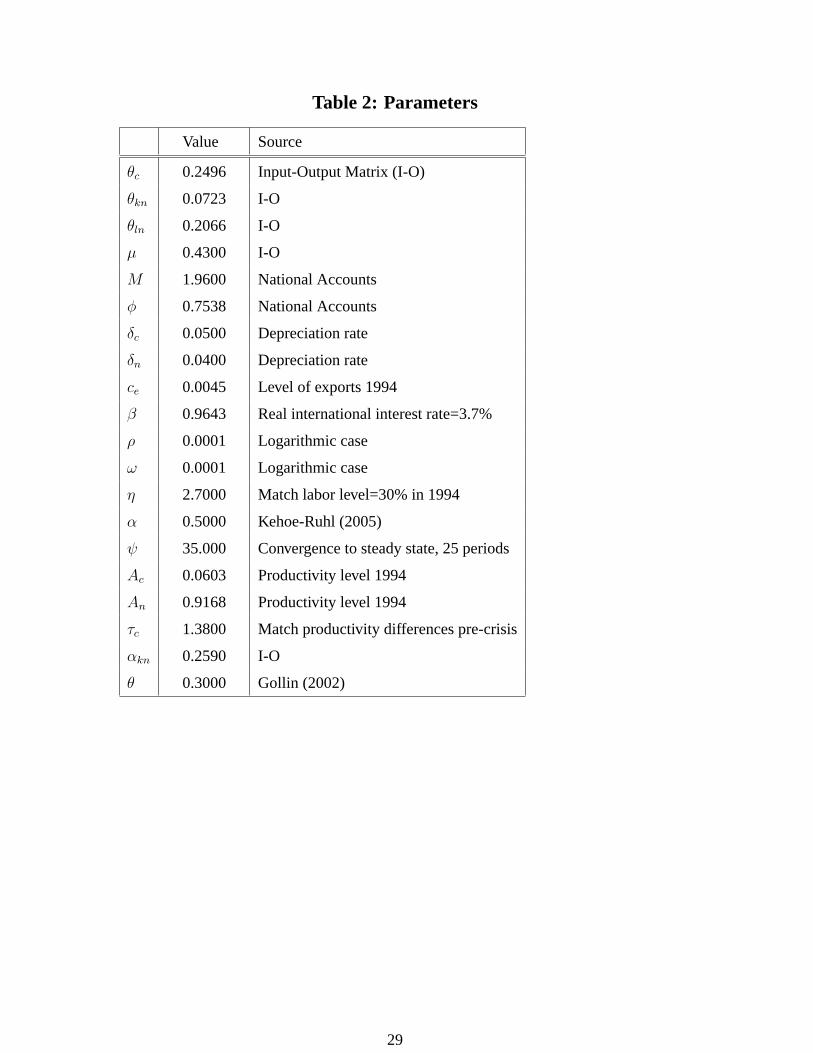
We summarize the calibration procedure and the values chosen in Table 2.
5 Experiments
In this section, we analyze the behavior of labor, productivity and output along a transition
path that is interrupted by a crisis. The initial period corresponds to 1994. We choose this year
because available data on interest spreads begins in that year. We set the initial capital stock in
27If we use the input-output matrix to calibrateθ, we find a value close to 0.30.28We have assumed in the data thatpc1997 = 1 andpm1997 = 1. In our baseline experimentpc1997 = 1.02 and
pm1997 = 0.99.
18
each sector to match the Korean economy in 1994. Also, we choose an initial level of foreign
debt such that the debt to real GDP ratio is equal to 11% in 1997.29
As a baseline, the crisis is represented by an unanticipated sudden stop, precluding any new
borrowing from the rest of the world for two periods. Simultaneously, the economy also faces
an unanticipated sequence of higher interest rates.
We compare detrended data with detrended model outcomes. We detrend model outcomes
in the same way we detrended the data, with the Hodrick-Prescott filter. We do this because
even though the model does not display long run growth, there is a transition towards a steady
state. We eliminate the effects of this transition.
5.1 Benchmark
Our baseline experiment is an unanticipated sudden stop together with an unanticipated in-
crease in interest rates. The sudden stop consists of eliminating any new foreign borrowing for
two periods. These periods correspond to 1998 and 1999 in the data. To construct the sequence
of interest rates, we follow Meza and Quintin (2006).30 In the experiment, we assume that the
values of interest rates are perfectly anticipated with one exception. The initial expectation of
interest rates for 1998 and subsequent periods is to match their 1994-1997 average in the data.
This value is 3.7%. After 1998 all expectations for interest rates are accurate and match the
data.31
Before displaying the results, we discuss the intuition behind them. The sudden stop of
capital inflows requires the economy to switch from negative to positive net exports. The
economy faces a downward sloping demand curve for its exports. As the economy is forced
to increase exports, their price, relative to the price of intermediate imported goods, falls. The
increase in the price of imports has a negative impact on the investment sector, reducing the
amount of labor it uses.
At the same time, there is a second effect that assists in the resource movements we docu-
ment. Investment falls sharply as international interest rates rise. This drives down the demand
for investment goods as resources used in investment can alternatively be sent abroad. Even
though exports increase as a result of the crisis, the fall in the remaining uses of investment
29Korea had a debt to GDP ratio of 11% in 1997, as reported by Lane and Milesi-Ferretti (2006).30We use data on interest rates on US Treasury bills, US inflation and a spread of Korean debt to calculate a
real international interest rate.31We solve the model assuming that a steady state is reached in finite time. This assumption provides us with a
system of nonlinear equations that we solve numerically.
19
goods is significantly larger. The overall result is a movement of resources, particularly labor,
from the investment to the consumption sector.
Because resources move into a less productive sector, the model is qualitatively able to
reproduce the behavior of key variables in the data after the Korean crisis. In the benchmark
experiment, both aggregate and approximate TFP fall. Real GDP and total labor also fall.
The behavior of total labor is unusual for a model of a sudden stop. We provide some
intuition for its behavior. In a one sector model, Chari, Kehoe, and McGrattan (2005) show
that the negative income effect due to the sudden stop leads to an increase in total labor supply.
The income effect is different in the investment sector of this model. The equilibrium condition
on labor in the investment sector is:
ln
(1 +
η
(1− φ)θnl
cnyn
)= (1− lc).
Labor in the investment sector depends on the ratio of investment sector consumption to invest-
ment sector gross outputcnyn
, and on labor in the consumption sector. The income effect works
through the consumption to output ratio. In our benchmark experiment, this ratio increases
as investment falls. The income effect leads to downward pressure on labor in the investment
sector.
Labor in the consumption sector in equilibrium satisfies:
lc
(1 +
η
φ(1− θc)(1 + τc)
ccyc
)= (1− ln).
The ratio of consumption to output in the consumption sector is always equal to one. This
eliminates from this sector any income effect. The coefficient that relateslc and(1 − ln) in
this last equation is strictly positive because the two labors are perfect substitutes. Therefore,
adjustments tolc andln after a sudden stop are negatively correlated, though movements inlc
are much smaller.
The key predicted outcomes are attached in Figures 8 and 9. All variables have been in-
dexed to take a value of 1 in 1997. In Figure 8 we compare data and predictions for aggregate
TFP, approximate TFP, labor in both sectors and real GDP. These variables are the main focus
of the paper. The effects are qualitatively correct but small.
In Figure 9 we compare data and predictions on other variables: exports, imports, terms
of trade and investment. In two aspects, the results of the numerical experiments are not qual-
itatively consistent with the data. The model predicts both a large increase in exports and a
significant worsening of the terms of trade for Korea in 1998. In 1998, neither showed much
movement in the data.
20
5.2 Shock to Export Demand
Our second experiment adds an additional shock to increase the cost of imported intermediate
inputs. The shock we use is a fall in export demand. This shock increases the driving force
behind our mechanism, which is that higher import prices force resources into less productive
sectors.
We again shock the economy with an unanticipated sudden stop and an increase in interest
rates. In addition, we assume a fall in export demand that leads to a corresponding worsening
of Korea’s equilibrium terms of trade. We do this by exogenously reducing the parameterce in
the export demand function.32 Our target for this change is to match the actual level of exports
demanded from the Korean economy in 1998. The shock to export demand captures directly
the fall in demand for Korean goods due to the region wide nature of the Asian financial crisis,
particularly the fall in demand from Japan.
Quoting Ghosh, Harmann, Lane, Phillips, Schultze-Ghattas, and Tsikata (1999):
“Growth of export volumes was dampened by further shocks to external de-
mand notably associated with the slowing of economic activity from Japan”.
The results from this experiment are qualitatively similar to our previous results, but are
quantitatively larger. They are attached as Figures 10 and 11. The fall in aggregate TFP is now
19.3% of the actual fall in aggregate TFP and the fall in approximate TFP is also larger. This is
because with fewer, more expensive imports the movements in labor are larger. In particular,
we see that the fall in labor in the investment sector is closer in magnitude to the observed fall
in the data than in the benchmark experiment. The model accounts for 37.6% of the fall in
labor in the investment sector. The model can also account for 14.8% of the fall in real GDP.
This experiment captures 60.4% of the fall for imports demanded by the Korean economy
in the data. A larger shock could potentially capture more of the fall. We ran an additional
experiment matching the fall in imports in the data. In this experiment, the fall in TFP was
39.7% of the fall in the data.
5.3 Shocks to the cost of working capital
In this experiment we use our original interest rate shocks but introduce an amplification mech-
anism. Specifically, we add working capital requirements as in Neumeyer and Perri (2005). In
the experiment, the addition of working capital requirements decreases labor supply in both
32Cavallo, Kisselev, Perri, and Roubini (2005) study financial crises with a shock to export demand.
21
sectors, but decreases labor supply in the investment sector more than in the consumption sec-
tor.
Working capital requirements require a change on the production side of the economy. We
modify the benchmark experiment by requiring firms in both sectors to borrow for the wage bill
in advance of production. Firms must set asidewjlj at the beginning of each period to hirelj.
In the process they forgo the opportunity to earn any interest on resources set aside so that the
cost to the firm of hiringlj iswj(1+ r)lj. The interest revenues are then collected and returned
to consumers in a lump sum manner. With this modification, profits in the consumption sector
equal:
pc(1 + τc)yc − wc(1 + r)lc − rckc.
In the investment sector, profits equal:
yn − rnkn − wn(1 + r)ln − pmm.
Results can be seen in Figures 12 and 13.33 In our experiment, both labor in consumption
and labor in investment fall, as in the data. Labor in investment falls 7.5%. Labor in consump-
tion falls 2.4%. The effects of working capital are larger in the investment sector than in the
consumption sector. The reason for this is that the consumer reduces capital accumulation,
because of consumption smoothing in response to working capital shocks. The model can ac-
count for 62.4% of the fall in labor in the consumption sector and 45.2% of the fall in labor in
the investment sector.
Working capital requirements increase the fall in TFP relative to the benchmark. In Fig-
ure 12, we see that measured TFP now falls 17.9% of fall in TFP experienced in the data.
Additionally, the model can account for 31.5% of the fall in GDP.34
Working capital requirements also improve the performance of the model relative to the
benchmark in terms of exports and terms of trade. These results are displayed in Figure 13.
Though exports still increase and the terms of trade worsen, both do so by a much smaller
amount than in the benchmark experiments. This is because, with the increase in the cost of
labor in the investment sector, it is more costly to increase exports.
33Because we are modifying the model, we recalibrateτc and the initial debt to continue matching previous
targets.34Neumeyer and Perri (2005) show that the addition of working capital requirements produces large falls in
output when interest rates rise.
22
5.4 Combined Experiment
We conclude the paper with an experiment that combines all of the effects studied so far. We
view this experiment as containing our main results. To conduct this experiment we add both
the shock to export demand and the working capital requirements to the benchmark experiment.
The results are attached as figures 14 and 15.
The results in this experiment are qualitatively similar to the previous experiment, but the
effects are larger. Labor in both sectors falls. The model can account for 53.2% of the fall
in labor in the consumption sector and for approximately 67.7% of the fall in labor in the
investment sector. In the case of TFP and GDP, the model can account for 30.0% and 41.0%
of the respective falls.
The model can account for 63.8% of the fall in imports. On the negative side, immediately
after the crisis, the terms of trade worsen by a substantial amount. Finally, the model predicts
a larger fall in investment than in the data and the previous two experiments.
5.5 Sensitivity Analysis
In this section, we report the results of the model under alternative parameter values. Particu-
larly, we are interested in different values for the elasticities implied by the model. The three
elasticities we vary are the elasticity with regard to imported intermediate goods, which is gov-
erned byα, the elasticity between the consumption goods, governed byρ, and the intertemporal
elasticity, governed byω. We measure the sensitivity of results in the combined experiment.
We vary the trade elasticity in both directions. Our baseline calibration gives an elasticity
of 2. We consider two alternative possibilities,α = { 110, 3
4}. This implies elasticities of10
9and
4. The results from this and all subsequent experiments are attached in Table 3. The effects
are significant for both experiments withα. However, they are more pronounced the smaller
α is. This is because as foreign imported intermediate goods and domestic intermediate goods
become more complementary, the rise in the cost of imports has a bigger effect.
The second parameter we consider is the elasticity between consumption goods. There is
little evidence on this elasticity. Our baseline elasticity is 1.0 which comes from a choice of
We also run sensitivity analysis overω. In the literature, a frequent value of the implied
intertemporal elasticity is12. This corresponds toω = −1. Loweringω does reduce the size
of the effects we report in our preferred calibration. TFP falls by a smaller amount. Labor
23
in the consumption sector falls by more and labor in the investment sector falls by less. The
reason for this is a substitution effect. Overall, consumption falls because of an income effect.
The substitution effect works against the fall in current consumption. The substitution effect is
determined by the price of the consumption sector good today relative to the price tomorrow,pat
pat+1. This ratio falls unexpectedly in 1998 as result of the crisis and rising import prices. When
ω is high, the consumer substitutes more consumption today for consumption tomorrow. When
ω is low, the consumer does not lower investment as much to take advantage of the relatively
cheaper price for today’s consumption sector good.
6 Conclusion
In this paper we first show evidence that the fall in TFP in Korea in 1998 is related to a real-
location of labor from a high productivity sector, manufacturing, to low productivity sectors,
especially agriculture and the public sector. We then suggest a mechanism that accounts for
both the sectoral reallocation and the fall in TFP in response to a sudden stop and an increase
in international interest rates. Our mechanism has two parts. First is the rise in the cost of
imported intermediate goods which are used predominantly in manufacturing. Second is the
fall in investment due to an increase in international interest rates.
Using a two-sector model, we have measured the quantitative impact of the sudden stop
combined with two additional shocks: a fall in export demand and an increase in the cost of
working capital. These forces can account for 30.0% of the fall in measured TFP after the
crisis. The mechanism can also account for 41.0% of the fall in real GDP.
We highlight one more point. Our analysis is conducted through a two sector small open
economy model with a consumption and an investment sector. This divide of the economy
contributes to reproducing the fall of aggregate labor. This is true even without working capital
requirements. There is no negative income effect on the supply of labor in the consumption
sector. Labor in the investment sector falls as the price of imports and international interest
rates rise. Consequently all our experiments predict a fall in aggregate labor.
24
Appendix: The Relationship between Sectoral Reallocation and LaborHoardingIn this appendix, we derive a relationship between our model and another model in the literature
used to account for a large fall in TFP in the case of the Mexican 1994 crisis.
Meza and Quintin (2006) model labor hoarding in a one sector model. Labor hoarding
allows the effort employees choose to adjust freely, while employment is costly to adjust.
The model can be used to measure TFP net of effort. Effort is unobservable to the economist
so it is measured through the model. In their model, TFP net of effort is,
TFPt =yt
kθt (ltεt)1−θ ,
whereεt represents effort. Variableyt represents a measure of output,kt is aggregate capital
(which can be adjusted for utilization) andlt is aggregate labor.
Equilibrium effort is equal to
εt =
(1− θ
f ν−1
ytlt
) 1ν
,
whereθ is the aggregate capital income share,ν > 1 determines the wage-elasticity of effort
andf > 0 is the average number of hours worked per worker. Bothν andf are parameters in
their model.
We now link this formula on effort to our research. Remember from a multi-sector model
that:
yt =∑i
piAitkθiit l
1−θiit .
We combine the last two equations to get:
εt =
(1− θ
f ν−1
∑i piAitk
θiit l
1−θiit∑
i lit
) 1ν
.
From here, we reinstate our assumptions in the measurement section that capital income shares
and depreciation rates are identical across sectors, and that factor markets are perfectly com-
petitive. Thus, sectoral capital to labor ratios are identical. It follows that
εt =
((1− θ
f ν−1
)((ktlt
)θ)(∑i
piAitlitlt
)) 1ν
.
There are three terms here. The first is a constant. The second is the aggregate capital to labor
ratio. In the case of Korea, this ratio grows after the crisis. Therefore, it cannot account for the
25
fall in TFP after the crisis. The third term is our term for approximate TFP. In the case under
study, we have already shown that changes in this term are due primarily to movements from
high productivity sectors to low productivity sectors. Labor reallocation in the data leads to
changes in measured effort.
References
BENJAMIN, D., AND F. MEZA (2006): “Productivity and Interest Rates in an Economy with
Financial Frictions: Facts and a Theory,” University of Southampton Working Paper.
CAVALLO , M., K. K ISSELEV, F. PERRI, AND N. ROUBINI (2005): “Exchange Rate Over-
shooting and the Cost of Floating,” Federal Reserve Bank of San Francisco Working Paper.
CHARI , V., P. J. KEHOE, AND E. MCGRATTAN (2005): “Sudden Stops and Output Drops,”
in American Economic Review, Papers and Proceedings, no. 2, pp. 381–387.
GERTLER, M., S. GILCHRIST, AND F. NATALUCCI (2003): “External Constraints on Mone-
tary Policy and the Financial Accelerator,” NBER Working Paper 10128, forthcoming Jour-
nal of Money, Credit and Banking.
GHOSH, A., J. HARMANN , T. LANE, S. PHILLIPS, M. SCHULTZE-GHATTAS, AND
T. TSIKATA (1999): “IMF-Supported Programs in Indonesia, Korea, and Thailand: A Pre-
liminary Assessment,” IMF Occassional Paper 178.
GOLLIN , D. (2002): “Getting Income Shares Right,”Journal of Political Economy, 110, 458–
474.
GREENWOOD, J., Z. HERCOWITZ, AND G. HUFFMAN (1988): “Investment Capacity Utiliza-
tion and the Real Business Cycle,”American Economic Review, 78(3), 402–417.
HORVATH, M. (2000): “Sectoral Shocks and Aggregate Fluctuations,”Journal of Monetary
Economics, 45(1), 69–106.
KEHOE, T. J.,AND K. J. RUHL (2005): “Sudden Stops, Sectorial Reallocations and the Real
Exchange Rate,” Working Paper.
LANE, P., AND G. M. MILESI-FERRETTI (2006): “The External Wealth of Nations Mark II:
Revised and Extended Estimates of Foreign Assets and Liabilities,1970-2004,” IMF Work-
ing Paper.
26
MENDOZA, E. G. (2006): “Endogenous Sudden Stops in a Business Cycle Model with Co-
lateral Constraints: A Fisherian Deflation of Tobin’s Q,” University of Maryland Working
Paper.
MEZA, F., AND E. QUINTIN (2006): “Financial Crises and Total Factor Productivity,” Federal
Reserve Bank of Dallas Working Paper.
NEUMEYER, P., AND F. PERRI (2005): “Business cycles in emerging economies: the role of
interest rates,”Journal of Monetary Economics, 52, 345–380.
NGAI , R., AND C. PISSARIDES(2006): “Structural Change in a Multi-Sector Model of Eco-
nomic Growth,” Forthcoming in American Economic Review.
OHANIAN , L. (2001): “Why Did Productivity Fall So Much During the Great Depression?,”
in American Economic Review, Papers and Proceedings, pp. 34–38.
OTSU, K. (2006): “A Neoclassical Analysis of the Korean Crisis,” IMES, Bank of Japan Work-
ing Paper.
RESTUCCIA, D., AND C. URRUTIA (2001): “Relative Prices and Investment Rates,”Journal
of Monetary Economics, 47, 93–121.
RUHL , K. (2005): “The Elasticity Puzzle in International Economics,” University of Texas-
Austin Working Paper.
27
Table 1: Input-Output Matrix
Input Final demand
Inv. sector Cons. sector TotalCons. Inv. Exports Imports Value added