MASTERARBEIT Titel der Masterarbeit „Towards multiple measurements of a single Bose-Einstein condensate by coherent outcoupling “ verfasst von Mira Maiwöger, BSc angestrebter akademischer Grad Master of Science (MSc.) Wien, 2015 Studienkennzahl lt. Studienblatt: A 066 876 Studienrichtung lt. Studienblatt: Masterstudium Physik UG2002 Betreut von: Univ. Prof. Dr. Hannes-Jörg Schmiedmayer
Transcript
MASTERARBEIT
Titel der Masterarbeit
„Towards multiple measurements of a singleBose-Einstein condensate by coherent outcoupling “
Betreut von: Univ. Prof. Dr. Hannes-Jörg Schmiedmayer
Abstract
This thesis deals with coherent output coupling as a method to probe the same cloudof ultracold atoms multiple times. We are especially interested in observing interferencefringes formed by atoms output coupled from a Bose-Einstein condensate (BEC) confinedin a double-well potential. Within this thesis output coupling from magnetic traps wasstudied with microwave- and radiofrequency radiation. Also, a laser system was built tooutput couple with two-photon Raman transitions. As our experiment uses magnetic trapswith spatially inhomogeneous magnetic fields, the second-order Zeeman shift gives rise toan effective potential that acts as a magnetic lens and (de)focuses the transverse densityprofiles of the output coupled clouds. This effect prevents the observation of interferencefringes from output coupled atoms. We expect to achieve this with the Raman lasersystem, based on the following two factors: First, we choose a spatial configuration of thetwo Raman laser beams such that photon-momentum is imparted onto the output coupledatoms. The atoms therefore leave the trapping region with strongly curved magnetic fieldsfaster. Consequently, we expect the effect of the magnetic lens to be weaker. Second, weexpect coupling strengths up to 1 MHz, which is three orders of magnitude stronger thanwhat we could achieve with microwave output coupling. This enables us to output couplewith short broadband pulses. Once we are able to perform phase measurements on afraction of output coupled atoms we can use this system to investigate phase diffusion orthe dynamics of the relative phase of BECs confined in double well potentials. Further wecan use output coupling to study the quantum measurement back-action on the BEC andrealize weak measurements on Bose-Einstein condensates.
Zusammenfassung
Die vorliegende Arbeit beschäftigt sich mit kohärentem Auskoppeln als Methode ummehrfach Messungen an demselben Bose-Einstein Kondensat (BEK) vorzunehmen. VonInteresse ist insbesondere die Beobachtung von Interferenzstreifen, geformt von wenigenAtomen, die aus einem Kondensat in einem Doppelmulden Potential ausgekoppelt wur-den. Im Rahmen dieser Arbeit wurde kohärentes Auskopplen mithilfe von Radiofrequenz-und Mikrowellenstrahlung untersucht. Außerdem wurde ein Laser System angefertigt, dasAuskoppeln mithilfe von zwei-Photonen Raman-Übergängen ermöglichen soll. Da unserExperiment Magnetfallen mit räumlich stark inhomogenen Magnetfeldern verwendet, führtder quadratische Zeeman-Effekt zu einem effektiven Potential, das ähnlich einer magnetis-che Linse die transversalen Dichteprofile der ausgekoppelten Atomwolken (de)fokussiert.Dieser Effekt verhindert bisher die Beobachtung von Interferenzstreifen in ausgekoppeltenAtomwolken. Wir erwarten jedoch, dass dies mithilfe des neu angefertigten Raman LaserSystems gelingen kann, begründet duch die folgenden zwei Faktoren: Erstens wird durchdie gewählte räumliche Konfiguration der beiden Raman-Laserstrahlen Photonen-Impulsauf die ausgekoppelten Atome übertragen. Die Atome verlassen die Fallenregion dadurchschneller. Wir erwarten, dass dies den Effekt der magnetischen Linse deutlich verringernkönnte. Zweitens erwarten wir Kopplungsstärken bis zu 1 MHz, etwa 3 Größenordnun-gen stärker als wir mit Auskopplung durch Mikrowellenstrahlung erreichen konnten. Diesermöglich die Auskopplung mit kurzen Breitband-Pulsen. Sobald es gelingt die relativePhase zweier BEK mithilfe von wenigen augekoppelten Atomen zu messen, kann diesesSystem beispielsweise zur Untersuchung von Phasendsiffusion oder der Dynamik der rel-ativen Phase von BEK in Doppelmulden Potentialen verwendet werden. Ein weiteresAnwendungsgebiet ist die Untersuchung der Rückwirkung der Messung auf das BEK unddie Umsetzung von schwachen Messungen an Bose-Einstein Kondensaten.
2.1 Energy level diagram for a two-level atom . . . . . . . . . . . . . . . . . . . 82.2 Rabi oscillations in a two-level atom for different detunings . . . . . . . . . 112.3 Damped Rabi oscillations in a two-level atom . . . . . . . . . . . . . . . . . 142.4 Energy level diagram for a three-level atom interacting with two light fields 152.5 Dressed state picture: Manifolds of uncoupled eigenstates of H0 + HL . . . 182.6 Eigenenergies of dressed and bare states with avoided crossing . . . . . . . . 20
The first experimental observation of Bose-Einstein condensation [1, 15] twenty years agoopened completely new possibilities for studying the properties of manybody quantumsystems. It is now possible to design cold atom experiments to simulate other systems.Ultracold gases are used as quantum simulators to address questions associated withcondensed matter physics, high energy physics or cosmology [24]. To give one example,neutral atoms in optical lattice potentials are used for quantum simulation of magneticordering (e.g [23, 57]). Another key application of Bose-Einstein condensates (BECs) ismetrology and inertial sensing [14]. As atoms are sensitive to gravitational forces andaccelerations, cold atoms are used as probes for inertial effects (among others) in atominterferometers. In a BEC all particles occupy the same single-particle quantum statewhich makes BECs a source of coherent matter waves analogous to a laser for light.The fundamental difference between a coherent state of photons and a coherent state ofatoms is the presence of atom-atom interactions in the latter. These interactions lead todephasing, which limits the coherence time and precision of a BEC based interferometer.On the other hand, the nonlinear nature of interparticle interactions provides a mechanismto create nonclassical states - squeezed atomic states with reduced fluctuations in someobservable - which can provide a coherent atomic source for precision measurements withhigher precision than can be achieved with classical input states [26]. These prospectsmake phase properties of BECs interesting to investigate on its own.
The achievement of Bose-Einstein condensation led to the developement of a varietyof experimental tools and techniques to trap, coherently manipulate and image cloudsof ultracold atoms [32, 43]. We now have the possibility to create BECs in small andcompact setups, for example on atom chips [19, 60] which are microfabricated wirestructures that produce the magnetic fields to trap and manipulate neutral atoms. Atomscan be detected to single-particle precision and good spatial resolution [11] which allowsa precise measurement of atom numbers and enables the detection of correlations inquantum degenerate systems. Most information on BECs is inferred from images of theatom distribution. The atom distribution is either imaged after ballistic expansion in timeof flight (tof) or in situ by dispersive imaging methods, like phase contrast imaging ordark-ground imaging. [32] When imaging in tof the entire cloud of atoms is dropped afterswitching off the trap and can only be imaged once in each experimental realization. Inorder to investigate the dynamics of properties that depend on initial conditions which arehard to control and reproduce precisely, one can either post-select the experimental data
1
Introduction 2
or do multiple measurements on the same sample of ultracold atoms [22, 49]. Multipleprobing schemes can for example be realized by changing the internal state of a smallfraction of atoms such that they become untrapped and can be imaged in tof, while theatoms remaining in the trap can be imaged at a later point in time. While post-selectingthe data naturally requires a large amount of data taking, multiple probing schemes arerestricted by the measurement back-action on the quantum system.
This thesis documents the first steps towards the realization of multiple probing schemes onthe Rubidium 2 (Rb2) experiment, an atomchip based experiment introduced in chapter 3of this thesis (or see references [4, 9]). We want to access information about the sameultracold system several times by coupling part of the atoms to an untrapped state. Theatoms will leave the trap and can be imaged before switching off the trap, releasing andimaging the remaining part of the BEC. The first goal is to implement a laser systemto output couple atoms which allows to infer the relative phase from a fraction of atomsof a BEC confined in a doublewell potential, to investigate its phase evolution and theback-action of the output coupling process on the remaining part of the BEC.
Before giving an overview of the structure of this thesis I will give a brief review of phasemeasurements of a BEC and methods to output couple atoms from a BEC.
Phase measurement of a BEC
Interference of two independent BECs In 1997 the observation of interference betweentwo 23Na BECs [2] which were created independently, released from their trap and allowedto overlap in tof was a first demonstration of macroscopic coherence properties of BECs.Atoms in a three-dimensional BEC (at zero temperature) are in a coherent state describedby a single wave function. The phase relation between two independently prepared con-densates is established in the measurement process. As Javanainen and Wilkens phrase it[30]:
[...] a measurement looking for interference of two condensates will find thecharacteristic consequences of the phase, even if there is no phase in the initialstate of the system.
The spatial overlap of the two atomic clouds in tof provides the same mechanism as therecombination at a beamsplitter. Two independently prepared condensates will showa definite value for their phase difference φ due to their intrinsic coherence properties.In each experimental run however, the phase differences will be completely randomlydistributed [13] and averaging over many experimental realization causes the fringecontrast to wash out.
When performing successive phase measurements on the same pair of condensates, thefirst measurement establishes a fixed phase relation between the two and the subsequent
2
Introduction 3
measurements show correlations in the relative phase of the condensates. This has beenshown in an experiment in 2005 [49] which continuously probed the relative phase of twoindependent BECs confined in optical doublewell potentials by stimulated light scattering.The experiment also showed that the evolution of the relative phase can be controlled byapplying an energy offset ∆E for a time ∆t. After a measurement that establishes thefixed phase relation between the initially independent condensates, their relative phase φevolves linearly as dφ/dt = ∆E/h, where h is Planck’s constant.
To understand how a fixed phase relation between two BECs establishes, we have to dig abit deeper: Phase difference φ and number difference n are canonical conjugate observables,they obey Heisenberg’s uncertainty relation ∆n∆φ ≥ 1, where ∆n denotes the variance ofthe number difference and ∆φ the variance of the relative phase. If we know the numberdifference between two BECs precisely, the relative phase is completely random. We stillcan observe interference between two independent BECs in each experimental shot asdescribed above, because of the overlap of their wavefunctions in tof. In the overlap regionwe cannot distinguish whether a single atom originates from one or the other BEC. Thisresults in an uncertainty in the number difference and allows the establishment of a fixedphase relation between the two BECs. In the case of two independently prepared BECs,we can however not assume that their phase relation exists prior to its observation.
Interference of coherently split BECs Coherent splitting of a BEC allows to create twoBECs with a well defined initial relative phase. This can be done by adiabatically splittinga magnetic trap on an atom chip into a doublewell potential by means of radiofrequency(RF) dressing [52]. If the doublewell potential has a well spacing and barrier height suchthat atoms can tunnel between the two wells, the BECs show a fixed relative phase, i.ethe measured phase difference is narrowly distributed. In reference [29], the interferenceof two coherently split and of two independently created BECs is compared for the sametrapping potentials. While the first show a narrow distribution of the relative phase, inthe latter the relative phase is randomly distributed.
Phase diffusion Fluctuations in the number of atoms in a BEC lead to decoherence. Asdiscussed above, for a BEC with a well defined atom number, its phase is indeterminate.In order to have a well determined phase, a BEC must be in superposition of states withdifferent atom number. As the mean field energy of a trapped BEC increases with the atomnumber N , the different number states have different energy and evolve at a different rate.They get out of phase, which limits the accuracy of a BEC interferometer. The timescaleon which this dephasing occurs is given by the phase diffusion rate which can be estimatedby [14]
Rφ = 1~
dµdN∆N
where µ is the chemical potential of the BEC. The phase diffusion rate is lower for number
3
Introduction 4
squeezed states, states with reduced fluctuations in the atom number difference comparedto coherent states. In reference [5], the implementation of a Mach-Zehnder type interfer-ometer for BECs split in doublewell potentials at the Rb2 setup is presented. It is shownthat the coherently split BECs exhibit reduced number fluctuations together with coher-ence times longer than expected for a coherent state. The creation of such spin squeezedstates is currently under investigation.
Output coupling from a BEC: atom lasers
We already stated that the coherence properties of a BEC resemble those of an opticallaser, with the key difference of the presence of interparticle interactions in the case of aBEC. Due to this resemblance, the term atom laser has been coined for propagating beamsof atoms coupled out from a BEC [47]. As an optical laser, an atom laser needs a trappedand macroscopically occupied lasing mode - the BEC - and some mechanism to couple thelasing mode to an untrapped mode. For BECs confined in magnetic traps, this is doneby coupling the atoms to a magnetically untrapped state. Atoms in the untrapped stateleave the trapping region under the influence of gravity and the mean-field potential of thestill trapped atoms. Raman output coupling can give the atoms an additional momentumkick away from the trapping region.
We now turn our focus to experimental techniques to couple atoms from a magneticallytrapped BEC to an untrapped state by changing the internal state of the atoms.
Output coupling without momentum transfer The first output couplers have been real-ized with RF pulses driving magnetic dipole transitions between the magnetically trappedand untrapped mF = 0 Zeeman states within the same hyperfine state. The first demon-stration of an atomlaser [37] used short RF pulses to output couple from a BEC of sodiumatoms. A quasi-continuous long pulse RF output coupler was demonstrated in 1999 [6]. RFoutput coupling mutually couples all the (in first order) equally spaced magnetic substates,i.e. an atom in the untrapped state can be coupled to the anti-trapped state.
Two-state coupling without momentum transfer, i.e coupling between magneticallytrapped and untrapped states of different hyperfine states, can be realized by a single-photon microwave (MW) transition [39, 47]. Here, the adressed states are closer to atwo-level system, since they have an energy difference in the order of the hyperfine split-ting (∆Ehfs/h ∼ 6.83 GHz in 87Rb), while the energy difference of magnetic substates isgiven by the linear Zeeman shift which is orders of magnitudes smaller (∆E/h ∼ 1 MHzfor small fields in 87Rb).
Output coupling with momentum transfer: Raman output coupling The couplingbetween a trapped and an untrapped state can also be realized with a two-photon Ramantransition. Two-photon Raman processes involve three atomic energy levels, the trapped
4
Introduction 5
state, the untrapped state and a virtual state close to an excited atomic eigenstate. Twolaser fields with a frequency difference ∆ω = ω1 − ω2 matching the energy splitting ofthe desired transition ∆E = ~ (ω1 − ω2) couple the trapped and untrapped state via thevirtual state. The atoms absorb a photon with frequency ω1 and are stimulated to emitone with frequency ω2. With each two-photon transition, momentum equal to ~(k1 − k2)is imparted onto the atom, where ki is the wave vector of the laser field. In contrast toRF output coupling, where one low-energy photon is exchanged, Raman transitions cangive a significant momentum kick to the atoms as they leave the trap. The first Ramanoutput coupler was demonstrated in 1999 [27].
In this thesis we document the setup of a Raman laser system (chapter 5) to be im-plemented into the Rb2 setup. It is designed to couple magnetically trapped and un-trapped states of different hyperfine levels in the 87Rb groundstate (|F = 1,mF = −1〉 ↔|F = 2,mF = 0〉). Further, we show the results obtained by RF- and MW output couplingfrom a BEC confined in a doublewell potential (chapter 4).
Structure of this thesis
This thesis is organized as follows:
• chapter 2 gives a theoretical description of the Atom-Light interaction in two- andthree-level atoms, including two-photon Raman transitions.
• chapter 3 describes the main components of the Rb2 experiment and provides theexperimental context for the work carried out for this thesis.
• chapter 4 summarizes the results obtained for RF- and MW output coupling.
• chapter 5 gives a detailed description of the laser system designed to drive two-photontransitions both between internal and external states.
• chapter 6 provides a conclusion and an outlook and describes the next steps towardsnon-destructive measurements of Bose-Einstein condensates in the Rb2 experiment.
5
2 Atom-Light Interaction
This chapter gives a theoretical description of the interaction of an atom with light. Westart by the description of a two level atom interacting with light and derive Rabi oscil-lations in a two level atom both for the undamped and damped case. The results will beused in chapter 4, for the analysis of the coupling of the two 87Rb hyperfine levels withmicrowave radiation. We will then look at the interaction of a three level atom with twolight fields and derive the effective coupling of two internal atomic states via a third level.This provides the theoretical basis for the Raman laser system presented in chapter 5.
2.1 Two level atom
2.1.1 Rabi oscillations
In a semiclassical approach, the atom is considered as a two level system interacting witha classical monochromatic light field.
Approximations
The interaction of atoms with light is a resonance phenomenon, meaning that if the fre-quency of the light is close to the frequency of a specific optical transition in the atom,the interaction will be strong. On the other hand, if the incident light is off-resonance, theatom - light interaction will be weak. Therefore atomic energy levels that are off resonancecan be ignored in a good first approximation, and the atom can be described as a two levelsystem interacting with light.
The second approximation made is the treatment of light as a classical electromagneticwave instead of a quantized field. This is valid if a large number of photons is interactingwith the atoms [21, 65], i.e if the photon number fluctuations of the electromagnetic fieldare small compared to the mean number of photons [41].
Time-dependent Schrödinger equation
We start by looking at the evolution of the state |Ψ〉 of the system, which follows thetime-dependent Schrödinger equation:
H |Ψ(t)〉 = i~∂ |Ψ(t)〉∂t
(2.1)
7
Atom-Light Interaction 8
ωg |g〉
ωe |e〉
ωrω0
∆
E/~
Figure 2.1: Energy level diagram for a two level atom with ground state |g〉 and excited state |e〉and corresponding energies ~ωg and ~ωe. ωr denotes the angular frequency of the electromagneticradiation and ω0 the resonance frequency of the transition |g〉 ↔ |e〉. ∆ is the detuning fromresonance ω0 − ωr.
We can split the Hamiltonian H in two parts: H = H0 +Hint(t). The time-dependent partHint(t) accounts for an external perturbation of the atom, in our case for the interactionof the atom with light.
Description of the two level atom The time-independent part H0 describes the unper-turbed atom, whose eigenstates are a groundstate |g〉 and an excited state |e〉. The unper-turbed Hamiltonian expressed in its eigenbasis is then given by H0 = ~(ωe |e〉 〈e|+ωg |g〉 〈g|)and has the following solutions:
H0 |e〉 = ~ωe |e〉
H0 |g〉 = ~ωg |g〉(2.2)
where ~ωg is the groundstate energy and ~ωe the energy of the excited atomic state. Wecan define the resonance frequency ω0 in terms of the two eigenenergies:
ω0 = ωe − ωg (2.3)
The internal state |Ψ〉 of the two level atom is expressed as a superposition of an excitedstate |e〉 and a groundstate |g〉:
|Ψ(t)〉 = be(t) |e〉+ bg(t) |g〉 (2.4)
Normalization requires that the coefficients be(t) and bg(t) satisfy|be(t)|2 + |bg(t)|2 = 1.
Description of the light field Now we consider the electromagnetic field interacting withthe atom. We assume it is monochromatic with angular frequency ωr:
8
Atom-Light Interaction 9
E(t) = εE0 cos(ωrt) = εE02(e−iωrt + eiωrt
)(2.5)
where E0 denotes the maximum amplitude vector of the electric field and ε its polarization.The spatial dependence of the field is ignored, we only describe the field at the positionof the atom. This is valid if we assume that the field is uniform over the extent of theatom and especially holds for optical transitions, where the wavelength λ of the field is inthe order of hundreds of nm, much larger than the size of the atom a0 in the order of Å.[20, 38, 55]
Electric dipole approximation The interacting part of the Hamiltonian within the electricdipole approximation is given by [16, 20, 65]
Hint = −d ·E (2.6)
where d is the atomic dipole operator in terms of the atomic electron position, d = −e · r,if we assume that the interaction is dominated by the interaction with a single electron.Using the completness relation |e〉 〈e| + |g〉 〈g| = 1 the dipole operator in terms of theatomic eigenstates |g〉 and |e〉 is
d = 〈g|d |e〉 |g〉 〈e|+ 〈e|d |g〉 |e〉 〈g| (2.7)
The diagonal matrix elements of the dipole operator are zero since 〈g| r |g〉 = 〈e| r |e〉 = 0,the odd position operator r only couples between states with different parity, i.e |g〉 and|e〉.
We define the coupling strength ΩR proportional to the off-diagonal dipole matrix elementssuch that
~ΩR = −〈g|d |e〉 εE0 (2.8)
Using these definitions the interaction Hamiltonian defined in Equation 2.6 can be writtenas
Equations of motion Inserting H0 and Hint and the ansatz in Equation 2.4 into theSchrödinger equation (Equation 2.1) and projection onto the eigenstates yields the equa-tions of motion for the coefficients be and bg:
9
Atom-Light Interaction 10
ibe(t) = ωebe(t) + Ω∗Rbg(t)
ibg(t) = ωgbg(t) + ΩRbe(t)(2.10)
To further simplify this expression, the variables bi(t) are transformed into ci(t) = bieiωit: asuitable phase for the variables bi(t) is chosen. This will only shift the zero-point energy andis algebraically equivalent to a transformation to a rotating frame [36, 53]. Using the reso-nance frequency ω0 defined in Equation 2.3 and decomposing cos(ωrt) = 1
2(e−iωrt + eiωrt),
the equations of motion become
ce(t) = − i2Ω∗Rcg(t)(ei(ω0+ωr)t + e−i(−ω0+ωr)t)
cg(t) = − i2ΩRce(t)(ei(−ω0+ωr)t + e−i(ω0+ωr)t)
(2.11)
We introduce the detuning ∆ of the laser frequency ωr from the resonance frequency ω0:∆ ≡ ω0 − ωr.
Rotating wave approximation (RWA) In the case of small detunings compared to thetransition frequency, i.e ∆ = ω0 − ωr ωr + ω0, the fast oscillating terms containingωr+ω0 can be neglected. They will average to zero when looking at a timescale associatedwith ω0 − ωr [16].
In our case, for 87Rb the energy splitting between ground state and first excited statecorresponds to ω0/2π = 384 THz [54] whereas lasers are detuned up to ∆/2π = 100 GHz,so this approach is justified.
Now those two coupled differential equations take a form that can easily be solved:
ce(t) = −iΩ∗R
2 cg(t)e−i∆t (2.12a)
cg(t) = −iΩR
2 ce(t)ei∆t (2.12b)
Differentiating Equation 2.12a and inserting Equation 2.12b yields
ce(t) + i∆ce(t) + ΩR2
4 ce(t) = 0 (2.13)
Rabi Oscillations We define the effective Rabi frequency Ωeff as
Ωeff =√
∆2 + ΩR2 (2.14)
10
Atom-Light Interaction 11
0 0.2 0.4 0.6 0.8 1 1.2 1.4 1.6 1.8 20
0.2
0.4
0.6
0.8
1
time t [2π / ΩR]
excitatio
nprob
ability|c
e(t)|2
Figure 2.2: Population of the excited state as described by Equation 2.16 for different detunings∆. At resonance (∆ = 0, black line); ∆ = ΩR (grey line); ∆ = 2ΩR (black dashed line).
Using the initial condition, that all the atoms are in the lower energy state |g〉, i.e. cg(t =0) = 1 and ce(t = 0) = 0, we get the following solutions for ce(t) and cg(t):
cg(t) = ei∆t/2[cos
(Ωeff2 t
)− i ∆
Ωeffsin(Ωeff
2 t
)](2.15a)
ce(t) = −ie−i∆t/2 ΩR
Ωeffsin(Ωeff
2 t
)(2.15b)
This means that the atomic state oscillates between |e〉 and |g〉. This behavior is calledRabi oscillation or Rabi flopping [21]. The probability of being in |e〉 is given by
|ce(t)|2 =( ΩR
Ωeff
)2· sin2
(Ωeff2 t
)(2.16)
When detuning the light field from the atomic resonance ω0, the frequency Ωeff of thisoscillation increases (see Equation 2.14) while the amplitude ΩR/Ωeff decreases. In orderto achieve a full population transfer of an ensemble of atoms, the light field needs to beresonant with the atomic transition. Figure 2.2 shows this behaviour for different detunings∆.
2.1.2 Damped Rabi oscillations
Density operators In order to take losses of coherence and spontaneous population decayinto account, the two level system is best described with the density matrix formalism. Wewill just briefly introduce the basics needed for the description of damped Rabi oscillations
11
Atom-Light Interaction 12
in a two level system with density matrices. A detailed introduction can be found intextbooks such as reference [50]. The density matrix ρ is defined as
ρ =∑i
pi |Ψi〉 〈Ψi| (2.17)
where pi describes the (classical) probability of the system being in one of the states |Ψi〉.The probabilities are normalized (
∑pi = 1) and the expectation value for any observable
A is expressed by the trace: 〈A〉 = tr(ρA). The density operator ρ also describes mixedstates and can account for incoherent processes.
Reformulating the problem above in this formalism gives the density operator for thesystem, using the state defined in Equation 2.4 with the matrix representation in the basis|e〉 , |g〉:
ρ = |Ψi〉 〈Ψi| =(ρee ρeg
ρge ρgg
)=(|ce|2 cec
∗g
cgc∗e |cg|2
)(2.18)
Equations of motion Since the time-derivatives of ce(t) and cg(t) have already beencalculated above, Equation 2.11 can directly be used to find the equations of motion forthe density matrix elements:
ρee = ∂t(ce · c∗e) = iΩR
2(ρ′eg − ρ′ge
)ρgg = −ρee = − iΩR
2(ρ′eg − ρ′ge
)ρ′ge = ∂t(cg · c∗e) = −i∆ρ′ge −
iΩR
2 (ρee − ρgg)
ρ′eg = ∂tρ′∗ge = i∆ρ′ge + iΩR
2 (ρee − ρgg)
(2.19)
where ρ′ge = ρgee−i∆t. We further used the normalization condition ρee + ρgg = 1⇒ ˙ρee = − ˙ρgg and ρ′ge = ρ′∗eg. Note that the density operator is a hermitian operator, i.eρge = ρ∗eg.
Population decay and decoherence We now add decay terms to model spontaneousemission and loss of coherence due to collisions. With ΩR = ∆ = 0 the terms have theform [55]
ρee = −Γρeeρgg = +Γρee
ρ′ge = −(Γ
2 + γc
)ρ′ge
ρ′eg = −(Γ
2 + γc
)ρ′eg
(2.20)
12
Atom-Light Interaction 13
The excited state population ρee decays at a rate Γ and the population in the ground stategrows at the same rate. These terms account for spontaneous emission from the excitedstate to the ground state. Γ = τ−1, where τ is the lifetime of the excited state. Theoff-diagonal terms or coherences ρ′ge = ρ′∗eg damp at a rate γ = Γ/2 + γc where the termΓ/2 is needed for consistency with the spontaneous emission. The additional dampingterm γc models decay beyond spontaneous emission. It models dephasing mechanisms,that do not change the state populations, such as collisions between the atoms. [55].
Optical Bloch equations We combine these damping terms (Equation 2.20) with theterms describing the time evolution due to the Hamiltonian (Equation 2.19) to get theoptical Bloch equations:
ρee = iΩR
2(ρ′eg − ρ′ge
)− Γρee
ρgg = − iΩR
2(ρ′eg − ρ′ge
)+ Γρee
ρ′ge = − (γ + i∆) ρ′ge −iΩR
2 (ρee − ρgg)
ρ′eg = − (γ − i∆) + iΩR
2 (ρee − ρgg)
(2.21)
A solution A general solution for the excited state population can be found for the caseof resonant light (∆ = 0) and setting γc = 0, i.e γ = Γ/2. With the initial conditionsρgg(t = 0) = 1 and ρge(0) = ρeg(0) = ρee = 0 the solution for the evolution of the excitedstate population ρee is [21, 35]
ρee = |ce(t)|2 = 12(1 + ξ2)
1−
[cos
(Ω′t)
+ 3ξ√4− ξ2 sin(Ω′t)
]e−
3γt2
(2.22)
where ξ = γ/ΩR is the ratio of damping to coupling and Ω′ = ΩR ·√
1− γ/4 the effectivecoupling. Figure 2.3 shows the oscillations between |g〉 and |e〉 for different damping factorsγ. Again, in order to achieve a full population transfer in an ensemble of atoms the ratioof damping factor to coupling strength ξ needs to be small.
2.1.3 Photon scattering rate
As discussed above, the optical Bloch equations (Equation 2.21) describe the excitation ofa two level atom by radiation close to a transition that decays by spontaneous emission.We can find steady state solutions (ρ = 0) to the equations to describe the excited statepopulation for times much larger than the lifetime of the exited state, for t Γ−1. Here,we assume that no collisions occur, i.e γc = 0 [35, 54]:
ρee = (ΩR/Γ)2
1 + 4(∆/Γ)2 + 2(ΩR/Γ)2 (2.23)
13
Atom-Light Interaction 14
0 0.5 1 1.5 2 2.5 3 3.5 40
0.2
0.4
0.6
0.8
1
time t [2π / ΩR]
excitatio
nprob
ability|c
e(t)|2
Figure 2.3: Population of the excited state as described by Equation 2.22 for different ξ. Blackline: ξ = 0, grey line: ξ = 0.1, black dashed line: ξ = 1.
The total photon scattering rate Rsc is proportional to the excited state population andthe decay rate of the excited state Γ:
Rsc = Γρee = Γ2
I/Isat
1 + 4(∆/Γ)2 + I/Isat(2.24)
Where the saturation intensity Isat is defined such that [54]
I
Isat= 2
(ΩR
Γ
)2(2.25)
2.2 Three level atom and Raman transitions
The goal of this thesis was to construct a laser system that can drive transitions betweenthe two hyperfine levels |F = 1〉↔ |F = 2〉 in the 87Rb ground state. For this we choose Ra-man transitions, which are two-photon processes that couple the two states, subsequentlydenoted as |0〉 and |1〉 via a far detuned, virtual state |e〉. Such two-photon processescan be used when the transition |0〉 ↔ |1〉 is electric dipole-forbidden, such as transitionsbetween different hyperfine states, or has an inconvenient frequency.[28]
We will see in chapter 5 that much stronger coupling between the two hyperfine levels ofthe 87Rb ground state can be achieved with a Raman transition than with a single photontransition in the microwave-regime for the powers we have available in our setup.
Interaction with two light fields In order to derive this coupling strength the model of athree level atom interacting with two light fields is used. Figure 2.4 shows the energy level
14
Atom-Light Interaction 15
ω0 |0〉
ω1 |1〉
ωe |e〉
ωr0
ωr1
∆0∆1
E/~
Figure 2.4: Energy level diagram for a three level atom interacting with two radiation fields ofangular frequency ωr0 and ωr1
diagram for such a model in a Λ-type configuration, where the energy of the intermediatelevel is higher than the one of the target states.
Hamiltonian of the system The problem is treated similarly as the one presented insection 2.1 and reference [28]. An atom with energy levels |0〉, |1〉 and |e〉 is perturbedby two light fields with angular frequency ωr0 and ωr1. Further it is assumed thatωr0, ωr1 ω1 − ω0, which means that each of the light fields cannot directly couple levels|0〉 and |1〉.
The Hamiltonian of the system is given by H = H0+H0int+H1
int, where the parts describingthe interaction Hint have the same form as in section 2.1:
H = H0 + H0int + H1
int =
= E0 |0〉 〈0|+ E1 |1〉 〈1|+ Ee + |e〉 〈e|
+ ~ cosωr0t(Ω0 |e〉 〈0|+ Ω∗0 |0〉 〈e|)
+ ~ cosωr1t(Ω1 |e〉 〈1|+ Ω∗1 |1〉 〈e|)
(2.26)
where Ωi is the coupling between |i〉 and |e〉 given by ~Ωi = Eidei, Ei being the amplitudeof the electromagnetic field and dei the dipole moment for the transition between |i〉 and|e〉.
Equations of motion and RWA Using the ansatz |Ψ(t)〉 = b0(t) |0〉+ b1(t) |1〉+ be(t) |e〉for the Schrödinger equation with the Hamiltonian in Equation 2.26 yields the equations
We introduce the detunings of the light fields with ωr0 and ωr1 from the atomic tran-sitions as follows: The detunings between the two lasers and the atomic transitions are∆0 = ωe−ω0−ωr0 and ∆1 = ωe−ω1−ωr1. The average detuning is given by ∆ = ∆0+∆1
2and the two photon detuning by δ = ∆0 −∆1.
We choose a frame rotating at e−iH′ t/~ with H ′ given by
H′ = ~
ω0 + δ
2 0 00 ω1 − δ
2 00 0 ωe −∆
(2.28)
Using the detunings defined above and applying the RWA (i.e dropping the terms thatoscillate at 2ωri), the equations of motion become
c0(t)c1(t)ce(t)
= − i2
−δ 0 Ω0
0 δ Ω1
Ω∗0 Ω∗1 2∆
c0(t)c1(t)ce(t)
(2.29)
where the state amplitudes bi(t) have also been transformed to the rotating frame, i.eci = bi(t)eiH′ t/~.
Adiabatic elimination Now it is assumed that the excited state |e〉 is initially not pop-ulated and since the light fields are far detuned by ∆, such that ∆ Ω0,Ω1, the changein the population of |e〉 can be neglected, i.e ce = 0. This step is known as adiabaticelimination. [28]
which can be substituted into Equation 2.29, yielding the reduced equations of motion forthe evolution of c0(t) and c1(t):
16
Atom-Light Interaction 17
(c0(t)c1(t)
)= i
2
δ + |Ω0|22∆
Ω0Ω∗12∆
Ω∗0Ω12∆ −δ + |Ω1|2
2∆
(c0(t)c1(t)
)(2.32)
The zero point energy is shifted by subtracting |Ω0|+|Ω1|4∆ from the diagonal terms:
(c0(t)c1(t)
)= − i
2
(−δe Ωe
Ω∗e δe
)(c0(t)c1(t)
)(2.33)
where the effective detuning is given by δe = δ − |Ω1|2−|Ω0|24∆ and the coupling strength
for the effective two level system consisting of levels |0〉 and |1〉, the two photon Rabifrequency is given by:
Ωe = −Ω0Ω∗12∆ (2.34)
The three level atom oscillates between the ground states at an effective frequency Ωe =√Ω2e + δ2
e and an amplitude given by Ω2e/Ω2
e. [16] This means, that a full population transferin an ensemble of atoms can be achieved even if the individual detunings ∆0 are ∆1 arelarge, as long as the effective detuning δe is zero.
We have seen in Equation 2.24 that the single photon scattering rate is proportional to∆−2 whereas the coupling between two groundstates of a three level atom is Ωe ∼ ∆−1
as just derived. By using far detuned laser fields, one can therefore suppress scatteringto the excited state and still achieve high two-photon Rabi frequencies. This will be themain argument to operate the laser for the Raman system detuned by ∆/2π =100 GHzfrom the 87Rb D2 - line.
Reference [28] derives solutions for the three level system described on the last pageswithout using adiabatic elimination to remove the excited state. The population in theexcited state will undergo oscillations at a higher frequency and a much smaller amplitudethan the oscillations of the populations in the groundstates. The amplitude and frequencyof |ce(t)|2 depends mainly on the ratio of the Rabi frequencies Ω0,Ω1 to the averagedetuning ∆. It is shown that for Ω0/∆ = Ω1/∆ = 10−1 and for δ = 0 the amplitudeof |ce(t)|2 is about 5% of the amplitude of |c0(t)|2 or |c1(t)|2. With the parameters wechoose for the Raman system Ω0/∆ ∼ /Ω1/∆ ∼ 10−3 we can assume that the adiabaticelimination is a valid approximation to describe our system.
2.3 Dressed state picture
In the dressed state picture, the state of the light field and internal atomic state aredescribed together. The coupling of an atom to the light field gives rise to new eigenstates,
17
Atom-Light Interaction 18
Figure 2.5: Manifolds of uncoupled eigenstatesof H0+HL. The energy spacing between the man-ifolds is ωL, the spacing between the eigenstates is~∆. Depending on the sign of the detuning statesconnected to |g〉 or |e〉 have a larger energy. Left:∆ > 0, right: ∆ < 0. For zero detuning, thestates |g, n〉 and |e, n− 1〉 are degenerate.
En−1
|g, n− 1〉
|e, n− 2〉
|e, n− 2〉
|g, n− 1〉
En
|g, n〉
|e, n− 1〉
|e, n− 1〉
|g, n〉
En+1
|g, n+ 1〉
∆ > 0
|e, n〉
|e, n〉
∆ < 0
|g, n+ 1〉
~ω
~ω
~∆ ~∆
the dressed states [41]. As in the beginning of this chapter, we use the model of a two levelatom with eigenstates |g〉 and |e〉 with resonance frequency ω0 and internal HamiltonianH0 (Equation 2.2).
Hamiltonian of the laser field The laser field is treated as a quantized field with creationand annihilation operators a† and a for photons in the laser mode. The Hamiltonian ofthe laser field with frequency ωL is
HL =(a†a+ 1
2
)~ωL (2.35)
The eigenstates of the light field are the photon number states |n〉, eigenstates of n = a†a,such that n |n〉 = n |n〉. As above, we assume that the laser intensity is high, i.e thenumber fluctuations are small compared to the mean photon number, ∆n 〈n〉.
The uncoupled states of the atomic field and laser field, the eigenstates of the HamiltonianH0 + HL are denoted as |g, n〉 and |e, n〉 (= |e〉 ⊗ |n〉, ’atom in |e〉 and n photons in thelaser mode’) with eigenenergies Eg,n = (n+1/2)~ωL and Eg,n = (n+1/2)~ωL+~ω0. Herewe choose the zero point energy such that ~ωg = 0. For small detunings ∆ = ωL − ω0,|∆| ω0, ωL these unperturbed eigenstates can be grouped in manifolds Mn of twoeigenstates |g, n〉 and |e, n− 1〉 separated by the detuning ~∆ around En. This is sketchedin Figure 2.5.
18
Atom-Light Interaction 19
Coupling We now add the interaction Hamiltonian in the RWA to the picture, i.e weneglect the terms a |g〉 〈e| and a† |e〉 〈g|.
Hint = ~Ω02(a |e〉 〈g|+ a† |g〉 〈e|
)(2.36)
Here Ω0 denotes the coupling strength for one photon between |g, 1〉 and |e, 0〉. The dipolematrix element between |g, n〉 and |e, n− 1〉 is
〈g, n| Hint |e, n− 1〉 = 〈e, n− 1| Hint |g, n〉 = ~Ω02√n ' ~ΩR
2 (2.37)
where the mean Rabi frequency is ΩR =√〈n〉Ω0. We can use this if we assume that
the light field is populated with a large amount of photons such that 〈n〉 ∆n and thematrix elements in the manifolds Mn+1 and Mn are almost the same. For a manifold Mn
the Hamiltonian then is:
Hn = En + ~2
(−∆ ΩR
ΩR ∆
)(2.38)
Dressed states Its eigenenergies are
E± = En ±~2
√∆2 + Ω2
R = En ±~2 Ω (2.39)
with generalized Rabi frequency Ω =√
∆2 + Ω2R. Its eigenstates are superpositions of the
states |g, n〉 and |e, n− 1〉:
|+, n〉 = sin θ2 |g, n〉+ cos θ2 |e, n− 1〉
|−, n〉 = − cos θ2 |g, n〉+ sin θ2 |e, n− 1〉(2.40)
with the dressing angle θ defined by
cos θ = −∆Ω, sin θ = −ΩR
Ω(2.41)
These are the dressed states, superpositions of of the uncoupled bare states |g, n〉 and|e, n− 1〉. Figure 2.6 shows the energy of the eigenstates depending on the detuning ∆with and without coupling. On resonance (∆ = 0) the bare states are degenerate, whilethe dressed states are separated by an energy difference ~ΩR and an avoided crossing isobserved.
19
Atom-Light Interaction 20
~ΩR
|−, n〉
|+, n〉
|g, n〉
|e, n− 1〉
−2 0 2−4
−2
0
2
4
∆[ΩR]
E±
[~ΩR
]
Figure 2.6: Eigenenergies of dressed (thick grey line) and bare states (black) depending on thedetuning. At zero detuning, the dressed states have an energy difference of ~ΩR and show anavoided crossing.
2.4 Momentum transfer
In this chapter we dealt with the change of an atom’s internal state due to optical tran-sitions. Due to momentum conservation, each time a photon of wavelength λ is absorbedor emitted by an atom of mass m, the atomic velocity changes by the recoil velocity vrec
given byvrec = ~k
m(2.42)
where k is the light’s wave vector with |k| = 2π/λ.
Two-level atom The interaction of light therefore not only couples the atom’s internalstates |g〉↔ |e〉, but also its momentum states |p〉 ↔ |p± ~k〉. For the dipole interactionconsidered above, the ground state in a given momentum state |g,p〉 couples to a singlemomentum state in the excited state |e,p + ~k〉.[16]
In coupling to a different momentum state, we have to take the change in the atom’skinetic energy into account, which will shift the resonance frequency ω0. The detuning∆ = ω0 − ωr defined above is only an approximated detuning, valid for an atom at restand neglecting the change in its kinetic energy due to the absorption of a photon. Wemodify it to take the atom’s momentum into account:
∆(p) = ∆ + p · km
+ ωrec (2.43)
where ωrec = ~k2
2m is the single-photon recoil frequency that accounts for the change in theatom’s kinetic energy. Note that we also took the change in the resonance frequency dueto the Doppler shift into account.
20
Atom-Light Interaction 21
Raman transitions For the three-level atom interacting with two light fields, we con-sider coupling between the states |0,p〉 ↔ |e,p + ~k0〉 ↔ |1,p + ~ke〉, where ki is thewave vector of the light field with frequency ωri and ke = k0 − k1. Here we assumethat the field with ω0 initially drives a photon absorption process and ω1 stimulates aphoton emission.[16] We redefine the detunings in the description of the three-level atominteracting with two light fields accordingly:
∆0(p) = ∆0 + p · k0m
+ ωrec0 (2.44a)
∆1(p) = ∆ + p · k1m
+ ωrec1 (2.44b)
The two-photon detuning δ is now
δ(p) = δ + p · kem
+ ωrece (2.45)
In the case of co-propagating laser beams and the resonance frequency much smaller thanthe frequency of the 2 laser fields, |k0| ' |k1| and ke ' 0. The two groundstates aretherefore coupled with almost no momentum transfer and the two-photon resonance ismomentum independent as δ(p) ' 0. Such a beam configuration is useful for couplinginternal states of an ensemble of atoms equally across their momentum distribution.
In any other configuration, momentum is transferred and the resonance is momen-tum dependent. The transferred momentum is p′ ∝ ke with absolute value given by|p′| = 2N~k sin(θ/2) for N two-photon events, where θ is the angle between the wavevec-tors of the two light fields k0 and k1 and |k0| ' |k1| = k [56]. This can be used tocouple different momentum states, for atomic velocity selection and to probe the atoms’momentum distribution [31].
21
3 The Rb2 Experiment
The Rubidium II (Rb2) experiment prepares clouds of ultracold Rubidium 87 (87Rb)atoms in magnetic wire traps created by an atom chip. The experiment was first built inHeidelberg in 2002 and moved to Vienna in 2007. A detailed description of the currentsetup can be found in the theses written in Vienna by T. Berrada [4] and R. Bücker [9]and the references therein.
In this chapter, some basic principles of magnetic trapping will be described. Then I willgive an overview of the experimental sequence and the imaging systems used to create,manipulate and image ultracold clouds or Bose-Einstein condensates of 87Rb atoms in thissetup.
3.1 Magnetic trapping of neutral atoms
The interaction energy of an atom with a magnetic dipole moment µ and a magnetic fieldB is given by [3]
V = −µ ·B (3.1)
The interaction with an external B-field breaks degeneracy of the atomic hyperfine levelsF and gives rise to 2F + 1 magnetic quantum numbers mF = −F, ..., F. For weakmagnetic fields, as long as the energy shift due to the interaction with the field is smallerthan the hyperfine splitting ∆Ehfs, the energy shift is linear in B. For 87Rb the hyperfinesplitting of the ground state is ∼ 6.83GHz and the linear Zeeman shift 0.7 MHz/G [54].
Additionally, if the angular Larmor frequency1 ωL = gFµB|B|/~ is large compared tothe rate of change of the field seen by the atom, the magnetic moment of the atom canadiabatically align to the magnetic field. The interaction then takes the form of a potentialdepending on the magnitude of the magnetic field.
V|F,mF 〉 = mF gFµB|B(r)| (3.2)
where µB is the Bohr magneton and gF the Landé factor.1In a semi-classical picture this can be pictured as the frequency of the precession of atomic dipole momentabout the quantization axis given by the external field
23
Context: Rb2 experiment 24
Wing’s theorem [63] states that it is not possible to create local field maxima in emptyspace, which is a direct consequence of Maxwell’s equations. In order to have a confiningpotential, the product gF ·mF has to be greater than zero to get attracted by field minima(states with gF ·mF > 0 are therefore named low field-seeking states). For 87Rb gF ' −1
2for the F = 1 ground state and gF ' 1
2 for F = 2. Therefore only the states |1,−1〉, |2, 1〉and |2, 2〉 can be trapped magnetically.2
3.1.1 Magnetic fields to trap atoms
The Rb2 experiment usually implements elongated magnetic traps: In the transversedirection of the trap (in the (x, y)-plane), the trapping potential is created by a DCcurrent I in a single wire on the atomchip along z together with a uniform Bias fieldBb = Bb · ex perpendicular to the wire created by external Helmholtz coils. A sketch ofthis configuration is shown in Figure 3.1. The longitudinal confinement is created by apair of wires perpendicular to the trapping wire on the atom chip (H-wires).
The transverse fields cancel at a distance d given by
d = µ0I
2πBb(3.3)
and define the trap center at a line parallel to the trapping wire for the low-field seekingatoms. The field created by the wire together with the Bias field Bb creates a quadrupolefield in the vicinity of the trap center. As the atoms are guided along the side of the wire,such a trap configuration is called a side-guide trap [19]. At the trap center, the magneticfield gradient is
∂B
∂r|r=d = 2π
µ0
B2b
I= Bb
d(3.4)
To avoid spin changing collisions to untrapped states (Majorana transitions [3]) in theregion of zero magnetic field an additional uniform offset field B0 = B0 · ez (Ioffe field) isadded in the longitudinal direction (along z). This completes the Ioffe-Pritchard configu-ration.
The harmonic trapping potential in the transverse direction is given by [4]
U⊥(x, y) = |gF | · µB ·B0 + 12mω
2⊥(x2 + y2)
ω⊥ =√|gF | · µBm ·B0
2πµ0I·B2
b (3.5)
2Remark concerning the notation: From now on, internal spin states |F, mF 〉 will simply be denoted likethis.
24
Context: Rb2 experiment 25
x
y
z
wire field +⊗
wire<
<<
bias field =
>
>
>
>
quadrupole field
d
Figure 3.1: Sketch of the trapping fields for the transverse confinement. A circular magnetic fieldcreated by the trapping wire (left) is combined with a uniform bias field (middle).
3.1.2 Radio-frequency dressing
Radiofrequency dressing enables us to create varying trap shapes. The principle is thesame as for optical dipole potentials: Coupling internal states of an atom to an externaloscillating field gives rise to new eigenstates and eigenenergies, dressed sates as describedin chapter 2.
As we couple magnetic substates in a static and spatially varying magnetic field Btrap(r)to a magnetic RF field BRF (r) oscillating at a frequency ω, its detuning δ from the atoms’local Larmor frequency ωL(r) is position dependent, and so is the coupling strength of theRF field, the Rabi frequency ΩRF = ΩRF (r). The energy of the dressed eigenstates at theposition r is [29, 40]
Vm′(r) = m′~√δ(r)2 + ΩRF (r)2 (3.6)
with
δ(r) = ωL − ωRF = µBgF~
Btrap(r) (3.7a)
ΩRF (r) = µBgF2~ Brf (r) (3.7b)
where Brf is the amplitude of the component of the RF field perpendicular to the localdirection of the static trapping field [52]. The energy of the dressed states acts as potentialfor the atoms as long as their magnetic moment can align to the local magnetic fieldadiabatically. Figure 3.2 illustrates the principle of RF dressing.
RF-dressing is used to realize trapping geometries beyond harmonic potentials, such asdouble well trapping potentials [29, 52]. It can also be used to engineer trapping potentialsfor optical clocks, such that the atomic clock transition is independent of the linear Zeeman-shift, improving the precision of an atomic clock [64].
On the Rb2 experiment a Mach-Zehnder interferometer has recently been implementedwith BECs confined in RF-dressed double well potentials [5]. Anharmonic trapping po-tentials with uneven level spacings can be created by means of RF-dressing and have beenused to control motional states of BECs to create twin-atom beams [10] or to implementa Ramsey interferometer with motional states [61].
25
Context: Rb2 experiment 26
mF = 1
mF = -1
RF
−2 0 2
−10
0
10
Position [a.u.]
Energy
[a.u.]
−2 0 2
−10
0
10
Position [a.u.]
Energy
[a.u.]
Figure 3.2: Principle of RF dressing: (left) two magnetic substates are coupled by a magnetic RFfield. (right) The eigenenergies of the dressed states form new potential minima. Image adaptedfrom [51]
3.2 Experimental Cycle
The preparation of the BEC takes place in a single vacuum chamber containing the atom-chip with viewports for the magneto-optical trap (MOT), optical pumping and imagingbeams. Two laser sources are used, one for each of the transitions between the hyperfineground states (52s1/2, F=1 and F=2) and the excited state (52p3/2) of 87Rb. The lasers arelocked through Doppler-free saturation spectroscopy setups. The frequency shifts neededto address the different hyperfine states (F’=(0,)1,2,3) of the excited state 52p3/2 areachieved with Acousto-Optic Modulators (AOMs). The energy level scheme of 87Rb withthe relevant optical transitions for our experiment are shown in Figure 3.3
Magneto-optical trapping The experimental sequence starts by collecting and precoolingatoms in a MOT [41]. Instead of the usual MOT configuration with six MOT beams anda quadrupole field, a mirror U-MOT as described in reference [62] is implemented: Twobeams are replaced by reflections from the chip surface. The magnetic field is created byU-shaped copper wires (see Figure 3.4) together with an external bias field. The MOT isloaded from background gas, where the Rubidium vapor pressure is increased by sendingcurrent through thermal dispensers. The atoms are optically cooled [36, 41] with light red-detuned (∼ 20 MHz) from the cycling transition |F = 2〉 ↔ |F ′ = 3〉 (’cooler’). Repumperlight resonant with the |F = 1〉 ↔ |F ′ = 2〉 transition brings the atoms into the cyclingtransition. In the MOT ∼ 108 atoms are cooled to T ' 200 µK in 18 s. [44]
Sub-Doppler cooling After the MOT is loaded, it is moved closer to the chip and com-pressed to match the position and size of the first magnetic trap. The magnetic fields areswitched off and the detuning from the cycling transition is increased (to ∼ - 70 MHz) forpolarization gradient cooling [41]. Due to high losses in the optical molasses the durationof this stage is short (∼ 4 ms [9]).
26
Context: Rb2 experiment 27
5p3/2
F’=3
F’=2F’=1F’=0
5s1/2
F=2
F=1
D2 line780.241 nm
repu
mp e
r
pumping
F=1
pumping
F=2
cooler
imag
ing
Figure 3.3: Hyperfine structure of Rubidium 87 (D2 line) with transitions used for cooling, opticalpumping and imaging in the experiment. Image adapted from references [4, 9]. Exact values forthe hyperfine splittings are given in [54].
Figure 3.4: (Left) atom chip with gold surface and micro-wires. (Right) copper structures underthe the chip. The Z-wire (green) is used for magnetic trapping after the molasses stage, the U-wire(blue) for the MOT stage and as an antenna for the RF radiation used for evaporative cooling.Either of the straight wires (red) can be used to create a field gradient for Stern-Gerlach separationof spin states in tof [4]. Image adapted from [9].
Optical pumping to |1,−1〉 At this point the atoms are in different spin states withinthe |F = 2〉 hyperfine manifold. To optically pump them into the desired |1,−1〉 state aweak magnetic field along x that defines the quantization axis is applied and two pumpbeams irradiate the atoms:A circularly polarized beam resonant with the |F = 2〉 ↔ |F ′ = 2〉 transition (’pumpingF=2’) brings the atom into the |F = 1〉 state . A second pump beam resonant with|F = 1〉 ↔ |F ′ = 1〉 (’pumping F=1’) irradiates the atoms along x with σ− polarizationwith respect to the quantization axis. The transition rules for σ− polarization imposes∆m = −1 for the excitation, so after many cycles of excitation and spontaneous decay(where ∆m = −1, 0, 1) the atoms will accumulate in |1,−1〉 where they are dark to bothpumping beams.
27
Context: Rb2 experiment 28
imagingatom chip
light sheet
absorption imaging beam
imaging
y
xz
objective
objective
Figure 3.5: Sketch of the imaging systems: The absorption imaging system images along x andrecords the shadow cast by the atomic cloud. The fluorescence imaging system images the atomsfrom below, along y, by collecting photons the atoms emit when passing through the light sheet.Figure adapted from [4].
Magnetic trapping and evaporative cooling Now the atoms are cold enough and in theright state to be trapped purely magnetically and further cooled by evaporative cooling.The first magnetic trap is created by a Z-shaped copper wire (Figure 3.4) under the chiptogether with external fields along x (Bb) and −z (B0) direction. The Z-trap first matchesthe position and size of the optical molasses and is then compressed to match the chiptrap. After compressing the trap the atoms are further cooled to degeneracy by evapora-tive cooling. Evaporative cooling relies on removing atoms from the cloud by inducingspin flips to an untrapped state with a ’RF-knife’. In a simplified picture, atoms withhigh energies are removed and the system rethermalizes to a lower temperature by colli-sions between atoms. A detailed description of the evaporative cooling ramp is given in [4].
After this preparation cycle, the Bose-Einstein condensates, typically containing a fewthousand atoms, are ready for manipulation with various radiation fields (e.g RF-dressingto split them in double well potential as described before or coupling to other internalstates as described in the next chapter) before they are imaged in tof with one of theimaging systems described below.
3.3 Imaging Systems
As in most of the ultracold atom experiments, experimental outcomes in the Rb2 experi-ment are probed by ’taking photographs’ of the atomic cloud. Two independent imagingsystems are implemented in the experiment: an absorption imaging system that imagesthe atoms in the (y, z) plane and a fluorescence imaging system imaging in the (x, z) plane.Both image the atoms in tof after switching off the trap, which means that for each exper-imental cycle the atomic cloud can only be imaged once. Figure 3.6 shows images taken
28
Context: Rb2 experiment 29
with both of the systems. The atoms are imaged with light resonant with the |F = 2〉 ↔|F ′ = 3〉 transition (’imaging’), which means that the atoms have to be pumped to the|F = 2〉 state before the imaging.
3.3.1 Absorption Imaging
With the absorption imaging system we can measure the density of the atom cloud in-tegrated over the radial imaging axis x. The atoms are illuminated with a σ+ polarizedimaging beam resonant with the |2, 2〉 ↔ |3, 3〉 transition and the shadow cast by theatoms is recorded by a charge coupled device (CCD) camera. Each atom scatters a fewhundred photons and attenuates the imaging beam. By comparing the intensity of theimaging beam Ii(y, z) to the intensity of the light that passed through the cloud If (y, z),the density of the atom cloud can be inferred from Beer-Lambert’s law:
If (x, y)Ii(x, y) = e−σ0·n(y,z) (3.8)
where n(y, z) =∫n(r)dx is the density of the cloud integrated over x and σ0 the resonant
scattering cross section of the used transition. For the chosen imaging transition |2, 2〉 ↔|3, 3〉, the resonant scattering cross section is σ0 = 2.91 · 10−9cm2.
During each cycle four images are taken: The first containing signal from both the atomsand the imaging beam (If ), the second tens of ms after the first to allow the atoms toleave the imaging region, and recording only the signal of the imaging beam (Ii). Afterreading out the camera two more images are taken without imaging beam. This allows tocorrect the images for stray light and background signal of the camera.
Due to the orientation of the imaging axis the absorption imaging system cannot capturetransverse features of the atomic cloud such as interference fringes created by a splitBEC in a double well potential [5]. It is mainly used for calibration and atom numbermeasurements and most of the ’actual results’ are obtained with the fluorescence imagingsystem described below.
3.3.2 Fluorescence Imaging
As sketched in Figure 3.5, the fluorescence imaging system images the atoms along y inthe (x, z) plane. It is also referred to as light sheet, since it is created by two counter-propagating laser beams with a vertical waist of ∼ 20µm. It is located ∼ 1 cm under thechip surface which corresponds to a tof of 46 ms for the atoms. Contrary to the absorptionimaging system where the tof can easily be adjusted between 2 and 25 ms, changing thetof for this system implies realignement of the optical paths and refocusing of the camera,therefore we work with fixed tofs of 46 ms. The atoms fall through the light sheet where
29
Context: Rb2 experiment 30
30 40 50 60 70
20
40
60
80
position (z) [pix]
posit
ion(y)[pix]
0
0.2
0.4
0.6
100 200 300 400
100
200
300
400
position (x) [pix]
posit
ion(z)[pix]
0
10
20
30
40
Figure 3.6: Exemplary images taken with the absorption imaging system (1 pix =3.44µm)after6 ms tof and the fluorescence imaging system (1 pix =4µm) after 46 ms tof.
each of the atoms spends ∼ 100µs and scatters ∼ 1000 photons. The camera, an electronmultiplying CCD (EMCCD) camera detects about 2 % of the scattered photons, whichcorresponds to a sensitivity of 15 detected photons per atom.
3.4 Bose-Einstein Condensates
After having described how BECs are prepared in the Rb2 setup, I will now give a brieftheoretical description of Bose-Einstein condensates, restricted to a mean-field descriptionof BECs in harmonic trapping potentials. A description of Bose-Einstein condensates ina double-well potential based on the Bose-Hubbard model can for example be found inreference [4].
The phenomenon of Bose-Einstein condensation was first described in 1924 by S. Bose andA. Einstein. They predicted that below a critical temperature, non-interacting Bosonswill macroscopically occupy the energy ground state of a given system. [42] This phasetransition occurs for
nλ3th ' 2.612 (3.9)
where n is the particle density and λth = (2π~2/mkBT )1/2 the thermal deBroglie wave-length for particles with mass m and temperature T . Physically, this condition meansthat a BEC starts to form when the size of the single particle wavefunction is in the orderof the inter-particle spacing n1/3.
We consider neutral atoms confined in a harmonic potential:
Vext = 12m
(ω2xx
2 + ω2yy
2 + ω2zz
2)
(3.10)
where m is the mass of the atom and ωi are the trapping frequencies in the three spatialdirections.
The energy ground state for a single particle in a harmonic trap is that of an anisotropic
30
Context: Rb2 experiment 31
harmonic oscillator: [42]
Ψ0(r) =(mω
π~
)3/4e−
m2~(ω2
xx2+ω2
yy2+ω2
zz2) (3.11)
where ω = (ωxωyωz)1/3 is the geometrical mean of the three trapping frequenciesωi. We can introduce the wave function describing the state of N non-interactingBosons as product state φ(r) =
√NΨ0(ri) [42]. The condensate density distribution is
n(r) = |φ(r)|2 = N |Ψ0(r)|2. For non-interacting particles, the condensate size is thereforeindependent of the particle number N and its size can be characterized by the harmonicoscillator length aho =
√~/mω.
Quantum scattering theory describes collisions between two identical Bosons as isotropicscattering events [42]. They are characterized by the s-wave scattering length as, and foraverage inter-particle spacings much larger than the scattering length, i.e na3
s 1 we canmodel weak atomic interactions by an effective potential U(r) = gδ(r−r′) with a couplingconstant g = 4πas/m.The time evolution of such a weakly interacting gas is described by a nonlinear Schrödingerequation, the Gross-Pitaevskii equation (GPE):
i~ ∂∂t
Φ(r, t) =(−~2
2m ∇2 + Vext + g|Φ(r, t)|2
)Φ(r, t) (3.12)
where the inter-particle interactions are treated as a potential term proportional to theBEC density |Φ(r, t)|2. The groundstate for a given harmonic trap is a stationary solutionof Equation 3.12 and can be found by setting Φ(r, t) = e−iµt/~φ(r), where µ is the chemicalpotential. [16] With this, the GPE is
µφ(r) =(−~2
2m ∇2 + Vext + g|φ(r)|2
)φ(r) (3.13)
For a large number of atoms and repulsive interactions, the kinetic energy term is smallcompared to the others. In the Thomas-Fermi approximation, the kinetic energy term isdropped and a solution to Equation 3.13 can be found [42]. The density is given by: [16]
n(r) = |φ(r)|2 = 1g
[µ− Vext] = n0
(1− x2
R2x
− y2
R2y
− z2
R2z
)(3.14)
where n0 = µ/g is the peak density and Ri the Thomas-Fermi radius defined below. Thedensity distribution described by Equation 3.14 is an inverted parabola in each direction,defined by Vext(r). For Vext(r) = µ, the density is zero and the extension of the BEC is in
31
Context: Rb2 experiment 32
each spatial direction is defined by the Thomas-Fermi radii:
R2i = 2µ
mω2i
= a2i
2µ~ωi
(3.15)
where ai is the harmonic oscillator length given by ai =√~/mωi. By normalizing the wave
function to the atom number N , a value for the chemical potential µ can be found:[42]
µ = ~ω2
(15Nasaho
)2/5(3.16)
Elongated traps On the Rb2 experiment highly anisotropic trapping geometries are usu-ally used, i.e traps with high aspect ratios up to ω⊥/ωz ∼ 300 [4], where ω⊥ = (ωxωy)1/2
is the transverse trapping frequency.
For the experimental data shown in the next chapter, we use traps with an aspect ratioof ω⊥/ωz ∼ 100, traps which are highly confined in the transverse direction, ω⊥/2π ∼ 2kHz, and weakly confined longitudinally, ωz/2π ∼ 20 Hz. For N ∼ 5000 atoms and withEquation 3.16 the chemical potential is µ ∼ h · 1 kHz.Condensates in such elongated traps are usually referred to as being in the 1D regime.The particles are in the transverse groundstate but populate many longitudinal modes.As their mean-field interaction energy or chemical potential is small compared with theradial level spacing, µ ~ω⊥, the condensates’ transverse degrees of freedom are frozen.
A way to describe the shape of 1D condensates within the mean-field approximation is byassuming that the radial and longitudinal degrees of freedom are decoupled [4, 42] and thewavefunction can be written as φ(r) = ψ(ρ)ϕ(z).If the interaction energy is small compared to the radial level spacing, µ ~ω⊥, theintereactions between the atoms can be neglected and the transverse wavefunction canbe approximated by a Gaussian, the non-interacting ground state for the radial harmonicpotential V⊥ = mω2
⊥ρ2/2. [42]
ψ(ρ) = 1π1/4a
1/2⊥
e−ρ2/2a2⊥ (3.17)
For the axial direction, as µ > ~ωz, the Thomas-Fermi approximation may be used to findthe longitudinal ground state wavefunction
ϕ(z) =√µ1Dg1D·
√1−
(z
R1D
)2(3.18)
The effective interaction parameter in 1D g1D is obtained by rescaling the interactionconstant g by averaging over the transverse density profile, such that g1D = g/2πa2
⊥ =2~ω⊥as [48]. The effective chemical potential µ1D is obtained by subtracting the groundstate energy E0
⊥ of the transverse wave function from the chemical potential, µ1D = µ−E0⊥
32
Context: Rb2 experiment 33
[4]. The longitudinal Thomas-Fermi radius in the 1D regime is
R1D =(3g1DN
2mω2z
)1/3(3.19)
The size of elongated condensates can therefore be be characterized by the transverseharmonic oscillator length a⊥ and the longitudinal Thomas-Fermi radius R1D. For typicalexperimental parameters within this thesis, a⊥ ' 0.25µm and R1D ' 25µm.
A detailed description of one-dimensional quasi condensates can for example be found in[48].
33
4 Output coupling test: MW and RF outputcoupling
As stated in the introduction (chapter 1), this thesis documents the first steps towardsthe realization of a probing scheme that allows to investigate properties of the same BECat different points in time. We want to do this by coupling a small fraction of atoms to amagnetically untrapped state, i.e a state with magnetic moment mF = 0 of the electronicgroundstate. Atoms in these states are to first order insensitive to magnetic fields andtherefore leave the magnetic trap and can be imaged independently from the remainingcloud of ultracold atoms. We want to use output coupling to realize a multiple probingscheme for the investigation of the dynamics of the relative phase of BECs confined indouble well potentials and to study the measurement back-action on the quantum system.
In the Rb2 experiment two systems that can couple the trapped |1,−1〉 state to an un-trapped state are already integrated: First, we can use the same RF source as for evap-orative cooling to couple the trapped atoms in |1,−1〉 to the untrapped |1, 0〉 Zeemansubstate. Second, a home-built microwave antenna [34] provides microwave (MW) radi-ation that can couple the trapped to the untrapped |2, 0〉 state.1 A third system, theRaman laser system described in chapter 5, couples the trapped state to the |2, 0〉 statewith two-photon transitions and is ready to be integrated into the experiment.
By testing output coupling with the two systems already implemented, we learn whichprospects and challenges lie ahead for the realization of multiple probing schemes with theRaman laser system. The MW field and the fields created by the Raman laser system cou-ple atoms to the same (internal) state, with the key difference of a significant momentumtransfer in the case of Raman output coupling.
In this chapter, we present the results obtained when output coupling from BECs confinedin single well and double well potentials with MW or RF radiation. We measured the MWcoupling strength for the powers currently available in our setup. Extracting the relativephase of split condensates in a double well potential from interference fringes formed byoutput coupled atoms could not yet be achieved. The challenge is that the clouds of atomsin the |2, 0〉 (|1, 0〉) state are (de)focused, which we attribute to an effective ’magnetic lens’effect due to the second order Zeeman shift in the trapping fields.
1’Radiofrequency’ refers to radiation with a frequency in the order of 1 MHz, i.e comparable to thelinear Zeeman shift of the magnetic substates in the 87Rb groundstates for a weak magnetic field (0.7MHz/G)[54]. ’Microwave’ radiation refers to frequencies in the order of the hyperfine splitting of thegroundstate (∼ 6.83 GHz)
35
Results - Output coupling without momentum transfer 36
F=2
F=1
mF = -2 -1 0 1 2
MW
RF
E/h
≈∼ 6.83 GHz
-y
E mF = −1
V−1
mF = 0
V0
~Ω
Figure 4.1: left: Energy level diagramm of the 87Rb groundstate with trapped |1,−1〉 statehighlighted in blue and untrapped |2, 0〉 (|1, 0〉) state highlighted in green (red). The trapped statecan be coupled to the |2, 0〉 state with MW radiation and to the |1, 0〉 state with RF radiation.right: Sketch of the potentials for magnetically trapped and untrapped states. The magneticallytrapped |1,−1〉 state experiences the potential of the harmonic trap and the mean-field potentialof the condensed atoms (V−1). The output coupled atoms experience the gravitational potential(gravity along y) and the mean-field potential of the still trapped BEC(V0) Adapted from [7].
4.1 Measurement of the MW coupling strength
We use two methods to measure the coupling strength or Rabi frequency attainable withthe radiation provided by the MW antenna already integrated into the Rb2 experiment:
• by scanning the MW pulse duration at constant amplitude and frequency we canextract the coupling strength from a model based on damped Rabi oscillations in atwo-level atom.
• by sweeping the MW frequency through resonance at different constant sweep ratesat constant amplitude we can infer the coupling strength from the Landau-Zenerparameter which relates the coupling strength to the sweep rate [37].
A detailed description of the microwave antenna that provides the MW radiation we useto output couple the atoms is given in [34]. In the following we characterize the frequencyof the MW field νMW with the detuning ∆MW from the hyperfine splitting ∆Ehfs of the87Rb ground state such that
∆MW = ∆Ehfs/h− νMW (4.1)
Double well potential The double well potential used to obtain the results within thischapter was created by RF-dressing (see subsection 3.1.2) the trap with a dressing am-plitude of rfamp = 0.65 in a ’splitting time’ of 10 ms. These settings were chosen becausethey provide double well potentials that usually give a high contrast in the interferencefringes. More details on double well potentials created in our experiment can be found inreferences [5] and [4].
36
Results - Output coupling without momentum transfer 37
905 910 915 9200
0.2
0.4
0.6
0.8
1
∆MW [kHz]
atom
numbe
r[a.u.]
single well
1174 1176 1178 1180 1182 1184 11860.4
0.6
0.8
1
∆MW [kHz]atom
numbe
r[a.u.]
double well
Figure 4.2: Trap bottom spectroscopy for left single well potential and right double well po-tential. The MW frequency νMW is defined w.r.t the hyperfine splitting of the 87Rb ground state∆Ehfs, such that ∆MW = ∆Ehfs/h− νMW . (MW amplitude: mw_ amp = 25, pulse duration t =2 ms.)
Trap bottom spectroscopy The resonance frequency is identified by scanning the fre-quency of the MW field and looking at the atoms remaining in the |1,−1〉 state. Atresonance, a maximum amount of atoms is coupled to the untrapped |2, 0〉 state. To avoidpower broadening we use a small MW amplitude.
4.1.1 Time scan
The first method to measure the coupling strength simply relies on scanning the MW pulseduration at maximum amplitude. The MW frequency is at resonance, as measured by thetrap bottom spectroscopy above. After shining the MW output coupling pulse onto theatoms we wait for 2 ms before switching off the trap. We then image the output coupledand released cloud after 6 (8) ms tof with the absorption imaging system described inchapter 3. Figure 4.3 shows exemplary absorption images taken with varying MW pulseduration. The holding time of 2 ms is sufficient to spatially separate the output coupledcloud from the cloud released after switching off the trap. As expected, the lower, outputcoupled cloud becomes brighter with increasing MW pulse duration.
Figure 4.4a and Figure 4.4b show the dependence of the atom number in the trapped|1,−1〉 and untrapped |2, 0〉 states on the MW pulse duration. We do not see oscillationsin the relative atom numbers but rather a saturation of the fraction of output coupledatoms. As the output coupled atoms leave the trap, we can model this with damped Rabioscillations. Comparing the experimental results to the theoretical description of dampedRabi oscillations (chapter 2), we can already estimate that the coupling strength is in thesame order of magnitude as the damping accounting for the loss of atoms in the untrappedstate as they leave the trap.
37
Results - Output coupling without momentum transfer 38
20 40 60 80
50
100
150
Position (z) [pix]
Posit
ion(y)[pix]
25 µs
20 40 60 80
50
100
150
Position (z) [pix]
225 µs
20 40 60 80
50
100
150
Position (z) [pix]
325 µs
20 40 60 80
50
100
150
Position (z) [pix]
1025 µs
Figure 4.3: Examplary absorption images (single shot) taken after MW irradiation of varyingpulse duration. The atom number in the untrapped state (lower region) increases with increasingpulse duration. 1 pix =3.44µm.
4.1.2 Fit models for the evolution of the untrapped population
When subjected to the output coupling pulse, the state of each atom, originally in thetrapped state, evolves into a superposition of trapped and untrapped states. In chapter 2we calculated the time-dependent probability for a two-level atom to get transferred toan excited state when interacting with a light field close to resonance with an atomictransition. We can use this model to extract the Rabi frequency or coupling strength fromour experimental data.
Beginning with a model based on the expression for damped Rabi oscillations in a twolevel atom as derived in chapter 2, we can equate the probability to be in the excited state|ce(t)|2 with the fraction of output coupled atoms u(t). As we are coupling two long-livingground states with the MW pulse, here the damping rate γ does not model spontaneousemission but rather a phenomenological decay rate accounting for the time in which theoutput coupled atoms leave the trap.
u(t) = |ce(t)|2 = 12(1 + ξ2) ·
1−
[cos(Ω′t) + 3ξ√
4− ξ2 sin(Ω′t)]
exp(−3γt
2
)(4.2)
where ξ = γ/Ω is the ratio between damping rate γ and coupling strength Ω. Theeffective coupling Ω′ is given by Ω′ = Ω
√1− ξ2/4.
In a second approach, we modify Equation 2.16 describing (undamped) Rabi oscillationsin a two-level atom. To account for the time in which the output coupled atoms leave thetrap, we include an escape time tesc that models a damping mechanism and an additionalparameter P corresponding to the fraction of atoms that remain trapped.
u(t) = P ·[1− exp
(− t
tesc
)]+ exp
(− t
tesc
)·( Ω
Ωeff
)2· sin2
(Ωeff2 t
)(4.3)
38
Results - Output coupling without momentum transfer 39
0 0.2 0.4 0.6 0.8 1 1.2 1.4 1.6 1.8 20
0.2
0.4
0.6
0.8
1
mw pulse length [ms]
relativ
eatom
numbe
r
(a) Single well: Relative ’trapped’ (blue) and output coupled (red) atomnumber as a functionof the MW pulse duration. Microwave pulse with maximum available amplitude (mw_ amp=44)and a frequency defined by ∆MW = 909 [kHz].
0 0.5 1 1.5 2 2.5 30
0.2
0.4
0.6
0.8
1
mw pulse length [ms]
relativ
eatom
numbe
r
(b) Double well: Relative ’trapped’ (blue) and output coupled (red) atomnumber as a functionof the MW pulse duration. Microwave pulse with maximum available amplitude (mw_ amp=44)and a frequency defined by ∆MW = 1180 [kHz].
Figure 4.4: Relative output coupled atom number depending on MW pulse duration. Outputcoupling from (A) single well, (B) double well
39
Results - Output coupling without momentum transfer 40
0 0.5 1 1.5 20
0.2
0.4
0.6
0.8
1
MW pulse duration [ms]
relativ
eatom
numbe
r
single well
datafit to Equation 4.5fit to Equation 4.3fitto Equation 4.2
0 1 2 30
0.2
0.4
0.6
0.8
1
MW pulse duration [ms]
double well
datafit to Equation 4.5fit to Equation 4.3fit to Equation 4.2
Figure 4.5: Fits to the output coupled fraction of atoms for BECs confined in single well anddouble well potentials. Blue: fit to Equation 4.5, green: fit to Equation 4.3, black: fit to Equa-tion 4.2
Here, the effective coupling Ωeff includes the detuning ∆ from resonance, Ωeff =√
∆2 + Ω2.As fit parameters P , tesc, Ω and Ωeff are used. ∆ is calculated from Ω and Ωeff .
In a third model, the output coupling process is described with a rate equation. Thisapproach is valid since the coupling strength is in the order of the output coupling ratewhich means that the atoms in the untrapped state leave the BEC before they flip backto the trapped state. The number of atoms in the BEC Nt evolves as [6]
dNt
dt = −Γ (Nt(t)−N0) (4.4)
where Γ ∝ Ω2 is the output rate. Solving this equation for the output coupled fraction ofatoms u yields
u(t) = P(1− e−Γt
)(4.5)
where P is again the maximal fraction of output coupled atoms.
4.1.3 Results
While a fit to the data with Equation 4.2 does not converge for longer pulse durations,a fit with Equation 4.3 yields good agreement with the experimental data as shown inFigure 4.5. The results of a fit to Equation 4.3 are summarized in Table 4.1.
For a BEC confined in a single well potential the fit yields an effective Rabi frequencyof Ωeff/2π = 720± 50 Hz and Ωeff/2π = 420± 70 Hz for double well potentials. For the
40
Results - Output coupling without momentum transfer 41
single well double wellatom number N 6130± 830 5200± 670Equation 4.3
Table 4.1: Summary of results Mean atom number and fit results for Figure 4.4a and Fig-ure 4.4b with Equation 4.3 and Equation 4.5
data taken in a single well potential, this results in a coupling strength Ω/2π = 380± 40Hz and ∆/2π = 600± 60 Hz. For double well potentials we extract a coupling strengthΩ/2π = 320± 60 Hz and ∆/2π = 270± 130 Hz. The output coupled fraction of atomstends to a stationary value of P = 0.92± 0.01 for single well potentials and P = 0.73± 0.02for double well potentials. The effective escape time extracted with this model istesc = 0.44± 0.02 ms for single well potentials and tesc = 0.51± 0.09 ms for double wellpotentials.
In contrary to Rabi oscillations in a two level atom, we are dealing with a many-bodysystem with a width in the order of the chemical potential µ ' h · 1kHz. ∆ shouldtherefore be interpreted as a factor modeling the width of the BEC. Similarly, tesc can beinterpreted as the pulse duration for which the Fourier width of the pulse t−1
esc ' 2 kHz isin the order of the chemical potential, i.e the entire condensate is addressed by the outputcoupling pulse.
4.1.4 Alternative measurement of the Rabi frequency
The atoms can also be coupled to the untrapped state by sweeping the MW frequencythrough resonance, by applying a MW pulse with varying frequency. We do this bychoosing a fixed time window (t=1 ms) in which the frequency is ramped up linearly intime over a given frequency range. By scanning this sweep range, we get different constantsweep rates dωMW /dt. The population in the untrapped state depends on the sweep rateand the coupling strength Ω as given by the Landau-Zener parameter Γ. With this scheme,the population in the untrapped state is given by [37]
u = 1− exp(−2πΓ)
Γ = Ω ·(
4dωMW
dt
)−1 (4.6)
41
Results - Output coupling without momentum transfer 42
0 20 40 60 80 100 1200
0.2
0.4
0.6
0.8
1
sweep range [kHz]
relativ
eatom
numbe
r
outcoupled fractionfit to Equation 4.6
Figure 4.6: Single well: Relative output coupled atomnumber depending on the MW sweeprange. Red: data, Green: fit to data with Equation 4.6. Maximum MW amplitude (mw_ amp =44)
By this method we measured the coupling strength for a condensate trapped in a singlewell potential. Figure 4.6 shows the output coupled fraction of atoms depending on thesweep rate and a fit to the data with Equation 4.6. The Rabi frequency extracted by a fitto the data is Ω = 1.38± 0.15kHz, which is a factor 4 higher than the result obtained byvarying the pulse duration.
4.1.5 Conclusion
We applied two methods to measure the Rabi frequency of the MW coupling at maximumavailable MW power. By scanning the MW pulse duration at a fixed frequency andamplitude we find that the coupling strength is Ω/2π ∼ 300− 400Hz for BECs confinedin single well and double well potentials. Sweeping the MW frequency through resonanceresults in a Rabi frequency Ω/2π ∼ 1.4kHz. A third value for the MW Rabi frequency isgiven in references [34, 44], where the Rabi frequency is extracted from a measurementof two-photon Rabi oscillations between the |1,−1〉 and |2, 1〉 state. It yields a couplingstrength Ω/2π ∼ 3kHz, which is another factor of two higher.
With the radiation provided by the MW antenna we can only achieve Rabi frequenciesin the order of possible detunings and decay rates, Ω ∼ ∆, t−1
esc, therefore the secondmethod relying on frequency sweeps through resonance is certainly more reliable since itis not affected by detunings from resonance and damping rates. For much higher couplingstrengths, i.e Ω ∆, tesc
−1, as we expect to attain with the Raman system presented inthe next chapter, scanning the pulse duration will be a suitable method to observe Rabi
42
Results - Output coupling without momentum transfer 43
200 400
200
400singlewell
posit
ionz[pix]
no output coupling
200 400
200
400
mw output coupling
200 400
200
400
rf output coupling
200 400
200
400
position x [pix]
doub
lewell
posit
ionz[pix]
200 400
200
400
position x [pix]200 400
200
400
position x [pix]
Figure 4.7: Exemplary fluorescence images taken (left) without output coupling pulse and witha (middle) MW output coupling pulse or a (right) RF output coupling pulse incident on theatoms. Top: single well. Bottom: double well. While interference fringes can be seen whenswitching off the trapping fields, they can not be observed in the clouds of output coupled atoms.Instead the transverse profiles are focused or broadened, depending on the internal state of theoutput coupled atoms. Images corrected for background noise and etaloning. Single shots, 1 pix=4µm.
oscillations.
4.2 Spatial profiles of output coupled clouds
Information about the spatial distribution of the output coupled atoms is obtained bythe fluorescence imaging system described in section 3.3. The atoms are imaged in thehorizontal (x, z) plane after 46 ms tof. Figure 4.3 shows examplary fluorescence images ofclouds dropped after switching off the trap, RF- and MW output coupled clouds. We canchoose to image the output coupled cloud or the cloud dropped after switching off thetrap by adjusting the camera trigger time. In order to spatially separate the two clouds,we use a holding time of 15 ms between applying the output coupling pulse and switchingoff the trapping fields. Figure 4.8 shows a scan of the camera trigger time for RF- andMW output coupled clouds, showing that we can image output coupled and droppedclouds individually by adjusting the camera trigger time as well as a (de)focusing of theoutput coupled clouds compared to the dropped clouds.
We could not observe interference fringes in the transverse direction when output couplingfrom BECs confined in double well potentials. Instead, we see a strong transverse focusing
43
Results - Output coupling without momentum transfer 44
30 40 50
100
200
300
400
500
LSTOF
posit
ionx[pix]
MW outcoupling
30 40 50
100
200
300
400
500
LSTOFpo
sitionx[pix]
RF outcoupling
0
100
200
300
400
500
Figure 4.8: Scan of camera trigger time (LSTOF). Left: double well, MW output coupling to|2, 0〉. Right: single well, RF output coupling to |1, 0〉. LSTOF < 35 ms: atoms in |2, 0〉 (|1, 0〉). 42ms < LSTOF < 48 ms atoms released after trap switch off. Transverse profiles (Integrated alongz), average over 5 shots, 1 pix =4µm.
of the MW output coupled cloud in the |2, 0〉 state. Its transverse width is reduced by afactor of ∼ 1.5− 2 compared to the width of a cloud released when switching off the trap.The RF-output coupled atomic cloud in |1, 0〉 is defocused, its transverse profile is ∼ 2− 4times broader than the one of the dropped cloud. This effect can be seen in single and indouble well trapping potentials (see Figure 4.9) We assume that this is the main reasonfor not observing interference fringes because the fringes can either not be resolved or arewashed out.
In the following, we will analyze this effect, which we attribute to the interaction of theoutput coupled atoms with the trapping fields and discuss the frequency dependence ofthe transverse profiles of RF- and MW output coupled clouds.
4.2.1 Effect of magnetic trapping fields
In the description of the interaction of the magnetic moment of an atom with an externalmagnetic field in the previous chapter (section 3.1) the second-order Zeeman shift hasbeen neglected since it does not contribute much to the energy of the trapped low-fieldseeking atoms: As described in chapter 3 the atoms are trapped in regions where themagnetic field is in the order of the offset field B0 ∼ 1 G. For the electronic ground state of87Rb, the linear Zeeman shift is 0.7 MHz/G, while the second order shift is ∼ 0.6kHz/G2
[54], three orders of magnitude smaller than the linear Zeeman shift. For the atomstrapped in regions with weak magnetic field gradients and curvatures the second-ordershift is therefore negligible. For atoms in a state mF = 0 there is no linear Zeeman shift,and the interaction of the output coupled atoms with the trapping field is dominated bythe second-order Zeeman shift.
44
Results - Output coupling without momentum transfer 45
0 100 200 300 400 5000
200
400
600
x [pix]
Fluo
.sig
nalintensit
y[a.u.]
single well
0 100 200 300 400 5000
100
200
300
400
x [pix]Fluo
.sig
nalintensit
y[a.u.]
double well
Figure 4.9: Averaged transverse profiles of atom clouds released after trap switch off (blue), MWoutput coupling (green) and RF output coupling (red). Left: Single well, right: double well. 1pix =4µm.
For alkalis in the groundstate the energy of an atom in an external magnetic field ofmagnitude B can be calculated analytically with the Breit-Rabi formula [8, 54]
E|F=I±J,m〉 = − ∆Ehfs2(2I + 1) + gIµBmB ±
∆Ehfs2
(1 + 4mX
2I + 1 +X2)1/2
X = (gJ − gI)µBB∆Ehfs
(4.7)
Here, ∆Ehfs denotes the hyperfine splitting of the ground state, gI and gJ are the Landéfactors associated with the nuclear spin I and the total electron angular momentumJ = S + L, where J = 1/2 for alkali ground states. The Breit-Rabi formula is valid formagnetic fields for which the atom’s energy shift is small compared to the finestructuresplitting. For weak magnetic fields, i.e. for B → 0 the eigenstates
∣∣∣F = I ± J,m⟩are
characterized by the projection of the total angular momentum F on the magnetic field|F,mF 〉. Note that for |2, 0〉 (upper sign) the energy increases while it decreases for |1, 0〉(lower sign). This is also shown in Figure 4.10.
The force due to an inhomogeneous magnetic field is [8]
F = −∂E∂B∇B (4.8)
Differentiating Equation 4.7 w.r.t B for m = 0 yields
45
Results - Output coupling without momentum transfer 46
F=2
F=1
magnetic field [G]
E/h[G
Hz]
0
0-25
5000
25
1500010000
Figure 4.10: Level structure of 87Rb in an external B-field. The levels highlighted in green andred correspond to states with mF = 0 for weak magnetic fields. Image adapted from reference [54]
−3−2
−10
12
x 10−5
−12−11
−10−9
−8−7
−6−5
−4
x 10−5
−25
−20
−15
−10
−5
0
x [m]
potential for F=1
y [m]
E [a.u]
−3−2
−10
12
x 10−5
−12−11
−10−9
−8−7
−6−5
−4
x 10−5
0
5
10
15
20
25
x [m]
potential for F=2
y [m]
E [a.u.]
Figure 4.11: Effective potential as given by Equation 4.7 for left atoms in |1, 0〉 and right atomsin |2, 0〉.
46
Results - Output coupling without momentum transfer 47
∂E
∂B= ±∆Eclock ·
1√1 +X2
·B (4.9)
where∆EclockB2 = ((gJ − gI)µB)2
2∆Ehfs= h · 575.15Hz/G2
is the second-order Zeeman shift between the two clock states for the 87Rb ground statein weak magnetic fields and X as defined in Equation 4.7. [54]
With this the force along x and y is
F = ∓∆Eclock ·1√
1 +X2·(Bx∂xBx +By∂xBy
Bx∂yBx +By∂yBy
)(4.10)
Calculation of paths of output coupled atoms The purpose of this calculation is tocheck whether the alteration of the width of the transverse profiles as shown in Figure 4.9can be attributed to the force due to the second-order Zeeman shift in the inhomogeneousmagnetic trapping field. The trajectories of the output coupled atoms in the transverse(x, y) plane are calculated under the influence of gravitational acceleration along y and de-pending on the internal state a repulsive or attractive force as described by Equation 4.10.The magnetic field was assumed to be that of an infinitely long and thin wire along z to-gether with a homogeneous field along x as shown in Figure 3.1 in chapter 3 to approximatethe transverse single well trapping potential.
The atoms’ position is initialized such that they lie on a circle of radius ∼ 1µm around thetrap minimum. The atoms’ initial velocity is vin = (2µ/m)1/2 with µ = h · 1 kHz. Thiscorresponds to the maximum kinetic energy attainable from atomic interactions when theatoms leave the trap center.
Comparison to width of transverse profiles We extracted the widths of the transverseprofiles by fitting a Gaussian to the data (see Figure 4.13). Assuming a Gaussian groundstate for the transverse profile, ψ(ρ) = 1
π1/4a1/2⊥
e−ρ2/2a2⊥ , the width of the cloud expanding
ballisticly in tof can be estimated by σ(t) = a⊥ · (1 + (ω⊥texp)2)1/2 [32], where texp isthe expansion time or tof. The fit yields a width of σ(t) = 38pix ' 0.15 mm whichcorresponds to a harmonic oscillator length of ameas
⊥ = 0.26µm after expansion in 46 mstof and a transverse trapping frequency of ω⊥ ' 2kHz, which is compatible with thecalculated harmonic oscillator length a⊥ = (~/mω⊥)−1/2 = 0.24µm. The FWHM of thefitted Gaussian to the profile of the dropped cloud is w ' 0.36 mm. For the MW outputcoupled the fit yields a FWHM of 0.2 mm.
In the case of the RF output coupled cloud we roughly approximate the width of the profileby the distance between the two peaks, resulting in a width of 1.32 mm. In Table 4.2 theFWHMs of the Gaussian fit to the data are summarized and compared to the calculation.
47
Results - Output coupling without momentum transfer 48
−1 0 1x 10⁻³
−0.01
−0.008
−0.006
−0.004
−0.002
0
x [m]
y[m
]
−1 0 1x 10⁻³
−0.01
−0.008
−0.006
−0.004
−0.002
0
x[m]
y[m
]
Figure 4.12: Paths of atoms in the (x, y) plane (left) without magnetic field influence, such asfor atoms released after switching off the trap (right) for output coupled atoms in the trappingfield. (Red) atoms in |1, 0〉, (green) atoms in |2, 0〉. The dashed line indicates the position of thelight sheet
0 200 4000
200
400
600
x [pix]
Fluo
.Sign
al[a.u.]
−1 −0.5 0 0.5 1
·10−3
0
20
40
60
80
position x [m]
atom
spe
rpixel
Figure 4.13: left: Averaged transverse profiles with Gaussian fit (black dashed lines) to the datato extract the width of the profiles. (blue) Cloud dropped after trap switch off, (green) MWoutput coupled clouds, (red) RF output coupled clouds. 1 pix =4µm. right: Calculated paths ofatoms. Contour plot of a histogram at light sheet position. The high peaks on the edges of theclouds are due to the initialisation of the calculation.
48
Results - Output coupling without momentum transfer 49
transverse width of calculationspatial profile (FWHM)
trap switch off 90 pix ' 0.36 mm 0.3 mmMW-outcoupling 50 pix ' 0.2 mm 0.2 mmRF-outcoupling 330 pix ' 1.32 mm 0.7 mm
Table 4.2: Comparison of widths of transverse profiles to calclulation of paths of output coupledprofiles
In the calculation, the second-order Zeeman shift ∆Eclock needs to be re-scaled by afactor of two to match the experimental observations. Figure 4.12 shows the result of thiscalculation. The spatial extension of the paths at the position of the light sheet agreeswell with the measured widths of the MW output coupled clouds and the clouds droppedafter switching off the trap.
We will see in the next section that the width of RF output coupled clouds dependsstrongly on the output coupling frequency. In order to model the width of the outputcoupled cloud precisely we would need to take both frequency and duration of the outputcoupling pulse into account.
Rescaling of the interaction with the trapping fields Although this simple modelconfirms the influence of the second-order Zeeman shift of the output coupled cloudsin the trapping fields, we had to rescale the interaction by a factor of two such that∆Ecalc
clock = ∆Eclock/2 to match the experimental observations. Several approximationshave been made in the calculation: Due to the initialization of the position of theatoms, we neglected the interaction with the magnetic field inside the BEC. Further, weneglected any interactions between the atoms expanding in tof and the finite size of thewire creating the trapping field.
A way to model our experimental observations more carefully is to numerically solve theGross-Pitaevskii equation (Equation 3.12) for the output coupled atoms as trapped in anexternal anharmonic potential given by the Breit-Rabi formula (Equation 4.7) for stateswith m = 0. In solving the GPE, the interactions with the still trapped BEC can betaken into account by the mean-field potential. Additionally, with such a simulation wecan check the influence of the momentum kick away from the trap center in the case ofRaman output coupling on the density distribution of the output coupled atoms.
4.2.2 Spatial profile of an atom laser
As already mentioned above, the spatial transverse profile of the output coupled cloudsdepends crucially on the output coupling frequency (also, see Figure 4.15). Due to itsfinite size, the trapped BEC extends over a region with different magnetic field strengths.
49
Results - Output coupling without momentum transfer 50
x [a.u.]
BEC
z [a.u.]
y[a.u.]
Figure 4.14: Sketch of output coupling resonance surface for an elongated BEC: The BEC (greyellipsoid) extends over a spatially varying magnetic field (black contour lines). Under the influenceof gravity, the condensate’s center is zsag = −g/ω2
⊥ below the field minimum. The thick black lineindicates the region where the output coupling pulse transfers atoms to a magnetically untrappedstate, the resonance surface. Left: Cut perpendicular to the long axis of the BEC, right: cutperpendicular to the transverse direction. Image adapted from [6].
The resonance frequency for spin flips from the trapped |1,−1〉 to the untrapped |1, 0〉state is given (to first order) by the linear Zeeman shift and as the magnetic field variesover the extension of the BEC, the resonance becomes position dependent. With short,broadband output coupling pulses, with a pulse duration such that the Fourier width ofthe pulse becomes comparable to the chemical potential of the BEC, the entire BEC canbe addressed and the output coupling is spatially independent [47]. With long outputcoupling pulses with a narrow Fourier width, a specific spatial region within the BEC isaddressed. Neglecting gravity, the resonance surface is an ellipsoid centered around thecondensate. Due to the gravitational sag, the resonance surface cuts through the BEC[6, 47]. This is illustrated in Figure 4.14.
When leaving the trapping region, the output coupled atoms interact with the remainingatoms. As the mean-field potential of the trapped cloud is not homogeneous over theoutput coupling surface the momentum of the output coupled atoms spreads. In aclassical picture, this would correspond to atoms rolling off a potential from differentheights [12]. When moving the resonance surface to the center of the BEC, the mean-fieldpotential gets stronger and transverse momentum spread and the width of the outputcoupled cloud larger.
The observed double peak structure is qualitatively consistent with the results presented in[12, 33, 46]. In [46] the transverse profile of an RF output coupled atomlaser is analyzedanalytically by optical methods in analogy to an optical laser and in [33] and [12] thetransverse profiles are modeled by numerically solving the GPE. As the output couplingfrequency increases, the resonance surface moves towards the margins of the BEC where themean-field potential is weaker and the transverse momentum spread of the output coupled
50
Results - Output coupling without momentum transfer 51
911 912 913 914 915 916
200
400
ωRF /2π [kHz]
x[pix]
single well
1178 1179 1180 1181 1182 1183
200
400
ωRF /2π [kHz]
double well
Figure 4.15: Scan of the output coupling frequency: (left) RF output coupling from a BECconfined in a single well and (right) from a BEC confined in a double well potential. Profilesaveraged over 5 shots, constant RF-amplitude and constant RF-pulse duration (τRF = 5 ms).Scan of the RF-frequency in steps of 100 Hz. 1 pix =4µm.
atoms decreases. The signature of this effect is the decrease of the distance between thetwo peaks as can be seen in Figure 4.15. In principle, the two peaks should merge at highoutput coupling frequencies, which we do not observe.
The data was obtained by scanning the RF-frequency in steps of 100 Hz with a constantRF-amplitude and a pulse length of τRF = 5 ms. The Fourier width of the pulse ∼ τ−1
RF =200 Hz is therefore smaller than the chemical potential of the BEC and by scanning theRF-frequency, we output couple from different spatial regions within the BEC.
Profiles of MW output coupled clouds
In Figure 4.16 and Figure 4.17 the dependence of the transverse profiles of MW outputcoupled clouds on the MW-frequency and MW-amplitude is shown. We used a pulseduration of τMW = 2 ms, the Fourier width of the pulse is therefore ∼ 500 Hz. We do notobserve a dependence of the transverse width of the output coupled clouds on the MW-frequency (Figure 4.16). This can be attributed to the magnetic lens which focuses the MWoutput coupled clouds. Further, the Fourier width of the MW-pulse is not significantlysmaller than the chemical potential and therefore the frequency-dependence of the outputcoupled profiles cannot be resolved. In choosing a long pulse duration, such that theFourier width of the output coupling pulse is smaller than the step size of the frequencyscan, we could check whether the magnetic lens suppresses the observation of a frequencydependence of the shape of the MW output coupled profiles.
Figure 4.17 shows the amplitude dependence of the MW output coupled profiles for singleand double well trapping potentials. For double well trapping potentials, we recover theexpected double peak structure as described in the last section. As for now, we do notunderstand, why we don’t observe a similar structure for clouds output coupled from a
51
Results - Output coupling without momentum transfer 52
1178 1180 1182
200
400
∆MW [kHz]
0
200
400
Figure 4.16: Transverse profiles of MW output coupled clouds (from a double well trappingpotential) depending on output coupling frequency at constant MW-amplitude (mw_amp = 28)and constant pulse duration, τMW = 2 ms. The MW frequency νMW is defined w.r.t the hyperfinesplitting of the 87Rb ground state ∆Ehfs, such that ∆MW = ∆Ehfs/h− νMW .
0 200 4000
1000
2000
x [pix]
Fluo
.Sign
al[a.u.]
single well
0 200 4000
200
400
x [pix]
double well
150 200 250 300 350100
200
300
400
x [pix]
double well zoom
20
30
40
Figure 4.17: Averaged transverse profiles of output coupled clouds at different MW amplitudes,with constant pulse duration τMW = 2 ms. (left) single well, ∆MW = 912 kHz. (center) doublewell, ∆MW = 1180 kHz. (right) zoom onto double peak structure. The colorbar indicates theMW-amplitude. 1 pix =4µm.
52
Results - Output coupling without momentum transfer 53
single well potential. An interesting amplitude dependence of the double peak structure isobserved for the clouds output coupled from a double well trapping potential: For smallMW-amplitudes the left peak is higher and with increasing amplitude the higher peak flipsto the right. This effect was reproducible, note that Figure 4.17 shows profiles averagedover 5 experimental realizations.
Conclusion
We now have an idea which challenges lie ahead for the observation of interference fringesfrom atoms output coupled from a double well trapping potential. We plan to model themagnetic lens more precisely and include the mean-field potential and output couplingfrequency in our calculation by numerically solving the GPE. In the next chapter, the Ra-man laser system is described, with which momentum is imparted onto the output coupledatoms such that they leave the trapping region faster. Once we have a better understand-ing of the output coupling process including the magnetic lens, we can check whether themomentum kick away from the trapping region will suffice to observe interference fringesfrom atoms coupled to the |2, 0〉 state.
53
5 Raman laser system
In this chapter the setup of the Raman laser system is presented, the construction ofwhich was the main goal for this master thesis. It is designed to drive Raman transitionsbetween the |1,−1〉 and |2, 0〉 states of the 87Rb ground state (52s1/2). The design is mainlyinspired by the work done by John E. Debs [16, 17] and we expect Rabi frequencies up to1 MHz, three orders of magnitude higher than achieved with MW coupling presented inthe previous chapter.
5.1 Principle
As we have seen in chapter 2, Raman transitions require two light fields with a stablefrequency difference that corresponds to the energy difference of the levels involved inthe wanted transition. As we want to drive Raman transitions between two hyperfinestates of the 87Rb groundstate, we require two light fields with a frequency difference∆ω/2π = ∆Ehfs/h ' 6.83 GHz. We want this frequency difference to be tuneable tosub kHz precision to address different energy shells within the condensate (as shown inFigure 4.14). Two laser beams with a frequency separation of ∼6.83 GHz can be producedby means of different methods: Two lasers relatively detuned by this frequency can bephase-locked (see e.g reference [58]) to yield a stable frequency difference. Another possi-bility is to modulate the laser current of a single laser which generates frequency sidebandsat the modulation frequency [45]. We have implemented yet another possibility using asingle laser together with an electro-optic modulator (EOM) as frequency shifting element.
As described in chapter 2, two-photon Raman transitions couple the two target states viaa third level. For a coherent Raman process, this level is not populated and thereforereferred to as virtual level. As we wish to suppress single photon transitions to the firstexcited state, each of the two laser fields should be far detuned from the 87Rb D2-line.The single photon scattering rate scales as ∆−2 (Equation 2.24) while the two-photon Rabifrequency is proportional to ∆−1 (Equation 2.34). By operating the laser red-detuned by∆/2π ' 100 GHz, we can strongly suppress the single photon scattering rates and stillachieve high two-photon coupling with the available laser powers.
We further require a fast switch to control the timing and pulse duration at µs precision,which we implement by using acousto-optic modulators (AOMs).
55
Raman laser system 56
52p3/2
F=2
F=1
∆ ∼ 100GHz
ω0
ωm, σ+
ωc, π
E/~
52s1/2
mF = -2 -1 0 1 2
Figure 5.1: Principle of Raman transitions. Energy level scheme of 87Rb with energy levelsrelevant for Raman transitions in our setup.
5.2 Setup
Figure 5.3 shows a scheme of our setup to drive Raman transitions. In the following partthe main elements are briefly described.
Light source
We use an external cavity diode laser (ECDL)1 in Littrow configuration operating at780.444 nm, about 100 GHz red-detuned from the 87Rb D2 line. The detuning or outputfrequency is tuned by adjusting the angle of the laser grating. We monitored the outputwavelength regularly to 0.005 nm precision and can exclude frequency drifts greater than2.5 GHz, the detuning is stable at least to 2.5%.
To avoid back-reflection into the laser diode, we use a polarization dependent opticalisolator. In the isolator the polarization of the beam is set by an input polarizer androtated by 45 in a magnetic field. The output polarizer is also rotated by 45 withrespect to the input polarizer. Back-reflected light is blocked by the input polarizer, asits polarization is rotated by 90 with respect to the input polarization as it passes themagnetic field twice. We could only achieve a maximal transmission of ∼ 70% of the opticalpower through the isolator right after the source due to differently polarized regions inthe beam. As we can couple the beam filtered by the optical isolator efficiently into theoptical fibers (typical efficiency of 50%), we still have enough output power to achieve highcoupling strengths with this setup. (see section 5.3)
1Toptica DL 100
56
Raman laser system 57
Electro-optic modulator
We use a fiber-coupled EOM 2 to generate the Raman beams with a frequency differencein the order of 6.83 GHz.
The operation of an EOM is based on the Pockels-effect, the dependence of the index ofrefraction of the used medium on the applied electric field. The change of the refractionindex ∆n depends linearly on the applied field E:
∆n = n30 · r · E (5.1)
for a material with refractive index n0 and electro-optic coefficient r. Light with wavelengthλ passing through a crystal of length L and thickness d will pick up a phase shift given by[59]
∆Φ = 2π∆nLλ
= πn30rLV
λd(5.2)
For a sinusoidal modulation of the applied voltage V (t) = V0 · cos(ωmt) at modulationfrequency ωm, the phase modulated field is then
EPM (t) = E0ei(ωct+m·cosωmt) (5.3)
where E0 is the amplitude and ωc the frequency of the unmodulated light field, the carrierfrequency. The modulation depth m depends on the driving voltage V0 and on a frequencydependent factor M(ωm) [59]
m = πn30rLV0λd
·M(ωm) (5.4)
The phase modulated signal can be decomposed using Bessel functions Jn(m).
EPM = E0
∞∑n=−∞
inJn(m)ei[(ωc+nωm)t] (5.5)
We can see that the phase modulated output of the EOM contains the carrier field withfrequency ωc and frequency sidebands at multiples of the modulation frequency ±nωm.For a modulation frequency satisfying kωm = ω0, where k is an integer number and ω0
is the resonant frequency of the Raman transition there will be pairs of sidebands inthe modulated beam that fulfill the resonance condition, i.e. the nth sideband togetherwith the (n + k)th sideband can drive Raman transitions between the desired levels.In practice, one will choose the modulation frequency such that either the first or thesecond-order frequency sidebands fulfill the resonance condition with the carrier, i.e k = 1
2Photline NIR-MPX800-LN10
57
Raman laser system 58
0 1 2 3 4 5
0
0.2
0.4
0.6
0.8
1
Modulation index m
J n(m
)2
J20
J21
J22
J23
Figure 5.2: Squared Bessel functions. The dashed lines indicate the choice of modulation depth,m = 2.4 where the carrier amplitude J0 is ideally zero.
such that |ωc − ωm| = ω0 or k = 2 such that |ωc − 2ωm| = ω0, as they contain most of theoptical power. This is also shown in Figure 5.2.
Considering the effective coupling between the two involved levels Ωe, which is proportionalto the amplitudes of the two driving fields over the detuning as shown in chapter 2 andconsidering all pairs of resonant sidebands we get
Ωe ∝E0E1
∆ ∝∞∑
n=−∞Jn(m)Jn+k(m) (5.6)
This specific sum of Bessel functions is zero for all m and k. [16, 17]. When tryingto drive Raman transitions directly with the phase-modulated output of an EOM, thecontributions of all resonant pairs of sidebands will destructively interfere and result inzero effective coupling.[17] It is therefore necessary to either separate the desired fre-quency sideband from the others, as can be done with an Mach-Zehnder interferometer asdescribed in reference [18] or to combine the modulated beam with a second unmodulatedbeam.
For the combination of modulated and unmodulated beam, it is important to minimizethe power in the carrier to suppress the formation of a standing light wave between theunmodulated beam at ωc and the carrier of the modulated beam [16]. Note that for amodulation depth m = 2.4 the carrier amplitude ideally is zero as shown in Figure 5.2. Wetested the EOM at a modulation frequency of ωm = ω0/2 ' 3.415 GHz and can suppressthe power in the carrier to 5% at a driving signal input power of 21 dBm. Each of the second
58
Raman laser system 59
frequency sidebands at ±2ωm = ±ω0 can then drive Raman transitions together with theunmodulated carrier. Since the modulation depth is frequency dependent (Equation 5.4),it remains to be tested whether a modulation at ωm = ω0 ' 6.83 GHz is favorable, i.eyields a higher ratio of total power in the resonant sidebands to power in the carrier.
Acousto-optic modulators
We use an AOM to control the timing and pulse duration of the Raman beams. In anAOM an incoming beam is diffracted at an acoustic wave which forms a travelling gratingin the modulator crystal, with a spacing given by the wavelength of the sound wave Λ.The nth order of the diffracted beam of wavelength λ comes out at an angle θ, that fulfillsthe Bragg condition sin(θ) = nλ/2Λ. Since the light is scattered at a moving wave, itsfrequency is Doppler-shifted by ∆ω = nωs, where ωs is the modulation frequency, thefrequency of the acoustic wave. We implemented the AOM driven at 80 MHz modulationfrequency in double-pass configuration, with a typical double-pass efficiency of 50%. Thedouble-pass configuration is necessary for tuning the modulation frequency of the AOMwithout realigning the beams. By implementing a second AOM which we can modulateat a frequency detuned from the first, we have the possibility to use the system in a Braggconfiguration, where we want to have the possibility to scan the modulation frequency ofthe AOMs.
Use as Bragg system Atoms at rest can be diffracted by a moving optical lattice createdby two laser beams of different frequency. Bragg scattering has been used to probe densityfluctuations of a system and to manipulate momentum states of BECs [56]. As describedin chapter 2, the interaction with a light field does not only couple the atoms’ internalstates, but can also be used to manipulate their external states by transferring momentumonto the atoms. The transferred momentum p′ is given by the Bragg condition |p′| =2N~k sin(θ/2), where N is the number of two-photon events and θ the angle betweenthe wavevectors of the two light fields. For atoms with initial momentum p, the relativefrequency of the two light fields ∆ω has to satisfy ~∆ω = p′2/2m + p · p′/m to couplemomentum states |p〉 ↔ |p′〉. In order to couple momentum states within the same internalstate one therefore needs a frequency difference of the two light fields in the order of therecoil frequency ωrec, as ~∆ω ∼ p′2/2m = ~2k2/2m = ~ωrec. For 87Rb, the recoil frequencyωrec is in the order of ' 10 kHz.
As the EOM is not suited for a modulation in this frequency range, we implement thesecond AOM.
59
Raman laser system 60
ECDL
Shutter Isolator
wavemeter
PBS
PBSPBS
wavemeter
Bragg beam
modulatedRaman beam
unmodulatedRaman beam
PBS
EOM
AOM
AOM
λ/2
λ/2
λ/2
λ/4 λ/4
Figure 5.3: Optical setup to create the beams required for driving Raman transitions betweenthe two hyperfine levels of the 87Rb groundstate. An additional AOM in double pass configurationgives the possibility to drive transitions in the Bragg regime. (λ/2... half wave plate, λ/4... quarterwave plate, PBS... polarizing beam splitter.)
5.3 Implementation into Rb2
Beam geometry
The Raman beams will be guided to the viewports of the vacuum chamber with identicalpolarization maintaining optical fibers to ensure that the two beams have the same trans-verse mode. In order to get higher beam intensities at the atoms and to avoid reflectionsoff the mirror of the atom chip, located ∼ 60 μm above the atoms, we need to focus thebeams. Figure 5.4 illustrates the beam geometry at the BEC: The unmodulated Ramanbeam shines π-polarized light with carrier frequency ωc onto the atoms along x, perpendic-ular to the long axis of the BEC. It will be focused by a cylindrical lens with focal lengthf=500 mm such that we get an elliptical Gaussian beam with a waist wy = 50μm alongthe vertical direction y and wz = 500μm horizontally. The second, modulated Raman
60
Raman laser system 61
zB0
x
yg
ωc, π
ωm, σ
+
ke
Figure 5.4: Sketch of proposed Raman beam geometry. The elongated BEC (grey ellipsoid) isilluminated by two Raman beams (red) perpendicular to each other. (Beam shape not realistic,for considerations concerning beam shape see text.) The net wavevector ke indicates the directionof the momentum kick the output coupled atoms get.
beam illuminates the atoms along z, along the long axis of the BEC and σ+-polarizedwith respect to the quantization axis defined by the magnetic field B0 (offset or Ioffefield). We focus the beam with a cylindrical lens with focal length f=500 mm to a waistwx = 50μm. The beam waists are therefore ∼ 10 times larger than the extension of thetrapped BEC, which can be estimated as a⊥ ∼ 0.25μm in the transverse direction andL ∼ 25μm longitudinally. This ensures that the trapped atoms are uniformly illuminated.
Expectations
Starting with an optical power of 70 mW after the optical isolator, we send ∼ 65 mWinto the first AOM in double pass configuration. We have a typical efficiency of 50%and have ∼ 32 mW optical power to split between unmodulated and modulated Ramanbeams. Both beams are coupled into optical fibers with a typical insertion loss of 50%.The modulation efficiency in the resonant frequency sideband is ∼ 20%. As the modulatedbeam gets focused much stronger, we need much more power in this beam to get aboutthe same intensities at the atoms. We propose to split the beam powers such that 24 mWgo into the unmodulated beam, yielding ∼ 12 mW after injection into the optical fiber,and 8 mW are sent into the EOM, yielding ∼ 0.8 mW in the resonant sideband.For the beam shaped with the cylindrical lense, we have an elliptical Gaussian intensityprofile
I(y, z) = I0 · e−2(y/wy)2 · e−2(z/wz)2(5.7)
Integration over y and z relates the total power in the beam P to the peak intensity I0:
P =∫ ∞
0
∫ ∞
0I(y, z)dydz = I0 · wy · wz
∫ ∞
0
∫ 2π
0e−2r2
rdrdϕ =π
2· wy · wz · I0
⇒ I0 =2 · P
π · wy · wz(5.8)
61
Raman laser system 62
To get an estimate for the single photon Rabi frequency, we use the definition in Equa-tion 2.25. The the single photon Rabi frequencies Ωi are related to the beam intensitiessuch that
Ω = Γ√
I
Isat(5.9)
For σ+-polarized light the saturation intensity is Isat ∼ 1.7mW/cm2 and for an circularbeam of size wx = 50µm with a total power of 0.8 mW yields a single photon Rabifrequency of Ω0/2π ∼ 4.7 · 105 kHz. For π-polarized light, the saturation intensity isIsat ∼ 2.5mW/cm2. The unmodulated beam shaped by a cylindrical lense to a waistwy = 50µm and wz = 500µm with a total power of ∼ 12 mW also results in a Rabifrequency of Ω1/2π ∼ 4.7 · 105 kHz. With the detuning ∆ ∼ 100 GHz we therefore expecta maximum two-photon Rabi frequency
Ωe = Ω0 · Ω12∆ (5.10)
of Ωe ∼ 1.1 MHz, which is three orders of magnitude higher than what we estimated forthe MW coupling strength described in chapter 4. The single photon scattering rate tothe first excited state is Rsc ∼ 30 Hz.This an estimate of the maximum available coupling strength. Note that the saturationintensity for circularly polarized light found in the literature [54] is for light resonant withthe |F = 2〉 ↔ |F ′ = 3〉 cycling transition, which is the transition that interacts strongestwith light. We will operate the laser far detuned from the D2-line, therefore the saturationintensity will be higher, resulting in a lower coupling strength. Second, we cannot knowthe intensities at the atoms precisely. Again, we calculated with upper bounds for thebeam intensities, assuming that there is no loss of beam power at the viewports of thevacuum chamber and that the beams are perfectly shaped Gaussian beams. Third, theformation of dressed states and their associated potentials (see chapter 2) can result in newbound states, which leads to a shutdown of the atom laser [16]. The practical boundaryfor the maximum coupling strength therefore remains to be investigated experimentally.
Photon recoil
As discussed in chapter 2, the output coupling process also transfers momentum onto theatoms. By choosing the output coupler geometry as described above, each atom undergoinga Raman transition into the untrapped |2, 0〉 state will get a momentum kick of p = ~ke.As the beams are aligned perpendicular to each other and |k0| ∼ |k1| = 2π/λ = k, thisresults in a momentum transfer of
√2~k at 45 with respect to the long axis of the BEC in
the horizontal plane. This gives the output coupled atoms an initial velocity of vin ' 8.3mm/s. We hope that this momentum kick will enable the observation of interferencefringes from output coupled clouds despite the magnetic lens due to the trapping fields.
62
Raman laser system 63
As the momentum kick brings the atoms into a region of smaller magnetic field gradients,we expect the magnetic focusing to be weaker than what we observed for clouds outputcoupled without momentum kick. We are planning to run GPE-simulations to checkwhether we can expect the output coupled atoms to form interference fringes when outputcoupled from a double well potential.
63
6 Conclusion and Outlook
In this thesis the first steps towards multiple measurements of the same ultracold system,especially probing the relative phase of a BEC confined in a double well potential, aredescribed. The goal is to infer the relative phase from interference fringes formed by asmall fraction of coherently output coupled atoms expanding in tof. Atoms from BECsconfined in magnetic traps can be output coupled by coupling them to a Zeeman sub-state with mF = 0, to an internal state which is in first order insensitive to magnetic fields.
We tested coherent output coupling with two systems integrated into the Rb2 experiment:by coupling the magnetically confined |1,−1〉 groundstate of 87Rb to the |1, 0〉 state withthe RF-radiation used for evaporative cooling and by output coupling to the |2, 0〉 statewith radiation provided by a home-built MW-antenna.
We could not yet observe interference fringes from atoms output coupled from a doublewell potential, but have gained some understanding of the effects that prevent thisobservation: We observed a (de)focusing of the transverse profiles of the clouds coupledto the (|1, 0〉) |2, 0〉 state compared to the transverse profiles of the clouds dropped afterswitching off the trap. We can attribute this to a repelling or attractive force due tothe second order Zeeman shift. The force is proportional to the magnetic field gradientF ∝ ±B∇B, which is strong near the chip trap. Second, we see that the transverseprofiles of the output coupled clouds depend crucially on the pulse duration and frequencyof the output coupling pulse, and our observations are consistent with results from othergroups concerning the transverse profile of an atom laser.
Further, we built a Raman laser system, that can couple the trapped |1,−1〉 to theuntrapped |2, 0〉 state with two-photon transitions. This system is ready to be integratedinto the Rb2 experiment and we expect coupling strengths up to three orders of magnitudehigher (Ω/2π ∼ 1 MHz) than what we can currently achieve with the MW-antenna. Thisgives us more flexibility in choosing the pulse duration and therefore the width of theoutput coupling pulse. We will direct the Raman beams perpendicular to each other ontothe atoms, giving them a momentum kick of
√2~k ' m · 8.3 [kg mm/s] away from the
trap center, at 45 with respect to the long axis of the BEC.
On the way to observe interference fringes formed by coherently output coupled atoms wesuggest to proceed with the following steps:
65
Conclusion and Outlook 66
• Setting up a simulation for the transverse density distribution of the output coupledclouds by numerically solving the GPE. The simulation should include the effectivetrapping potential for 87Rb atoms in the |2, 0〉 and |1, 0〉 state due to the secondorder Zeeman shift and the momentum imparted onto the atoms by the Ramanlaser beams. The goal of such a simulation is to find output coupler settings whichallow to infer a relative phase from interference fringes formed by the output coupledcloud. We should check whether short broadband pulses or spatially selective longpulses are favorable for our purposes.
• Implementing the Raman laser beams into the Rb2 experiment as described in chap-ter 5, followed by a careful calibration, i.e a measurement of the coupling strength. Atthis point we can hopefully observe interference fringes from output coupled atoms.If not, we have to think about other ways to deal with the magnetic lens. One ideais to use RF-dressing to create a coherent superposition of the |1, 0〉 and |2, 0〉 statein the output coupled cloud such that the effect of the magnetic lens averages out.
• Once we can observe interference fringes from output coupled atoms we can directlyuse the system to study phase diffusion and the evolution of the relative phase ofBECs confined in double well potentials. Further we can use the Raman system toexperimentally investigate evaporative cooling in 1D systems, i.e. to study the effectof strong output coupling on the temperature of the remaining cloud [25].
In the long term, coherent output coupling may be used to study the measurement back-action on the original BEC and to realize weak measurement schemes for the relative phaseof two (independent or coherently split) BECs.
66
Bibliography
[1] M. H. Anderson, J. R. Ensher, M. R. Matthews, C. E. Wieman, and E. A. Cor-nell. Observation of Bose-Einstein Condensation in a Dilute Atomic Vapor. Science,269:198–201, 1995.
[2] M. R. Andrews. Observation of Interference Between Two Bose Condensates. Science,275(5300):637–641, 1997.
[3] T. H. Bergeman, P. McNicholl, J. Kycia, H. Metcalf, and N. L. Balazs. Quantizedmotion of atoms in a quadrupole magnetostatic trap. Journal of the Optical Societyof America B, 6(11):2249, 1989.
[4] T. Berrada. Mach-Zehnder interferometry with interacting Bose-Einstein condensatesin a double-well potential. PhD thesis, Technische Universität Wien, 2014.
[5] T. Berrada, S. van Frank, R. Bücker, T. Schumm, J.-F. Schaff, and J. Schmiedmayer.Integrated Mach-Zehnder interferometer for Bose-Einstein condensates. Nature com-munications, 4:2077, 2013.
[6] I. Bloch, T. Hänsch, and T. Esslinger. Atom Laser with a cw Output Coupler. PhysicalReview Letters, 82(15):3008–3011, 1999.
[7] I. F. Bloch. Atomlaser und Phasenkohärenz atomarer Bose-Einstein-Kondensate. PhDthesis, Ludwig-Maximilians-Universität München, 2000.
[8] G. Breit and I. Rabi. Measurement of Nuclear Spin. Physical Review, 38(11):2082–2083, 1931.
[9] R. Bücker. Twin-atom beam generation in a one-dimensional Bose gas. PhD thesis,Technische Universität Wien, 2013.
[10] R. Bücker, J. Grond, S. Manz, T. Berrada, T. Betz, C. Koller, U. Hohenester,T. Schumm, A. Perrin, and J. Schmiedmayer. Twin-atom beams. Nature Physics,7(8):608–611, 2011.
[11] R. Bücker, A. Perrin, S. Manz, T. Betz, C. Koller, T. Plisson, J. Rottmann,T. Schumm, and J. Schmiedmayer. Single-particle-sensitive imaging of freely propa-gating ultracold atoms. New Journal of Physics, 11(10):103039, 2009.
67
Bibliography 68
[12] T. Busch, M. Köhl, T. Esslinger, and K. Molmer. Transverse mode of an atom laser.Physical Review A, 65(4):043615, 2002.
[13] Y. Castin and J. Dalibard. Relative phase of two Bose-Einstein condensates. PhysicalReview A, 55(6):4330–4337, 1997.
[14] A. D. Cronin, J. Schmiedmayer, and D. E. Pritchard. Optics and interferometry withatoms and molecules. Reviews of Modern Physics, 81(3):1051–1129, 2009.
[15] K. Davis, M. Mewes, M. Andrews, N. van Druten, D. Durfee, D. Kurn, and W. Ket-terle. Bose-Einstein Condensation in a Gas of Sodium Atoms. Physical Review Letters,75(22):3969–3973, 1995.
[16] J. E. Debs. The Application of Bose-Einstein Condensates to Inertial Sensing. PhDthesis, The Australian National University, 2012.
[17] J. E. Debs, D. Döring, N. P. Robins, C. Figl, P. a. Altin, and J. D. Close. A two-stateRaman coupler for coherent atom optics. Optics Express, 17(4):2319, 2009.
[18] I. Dotsenko, W. Alt, S. Kuhr, D. Schrader, M. Müller, Y. Miroshnychenko, V. Gomer,A. Rauschenbeutel, and D. Meschede. Application of electro-optically generated lightfields for Raman spectroscopy of trapped cesium atoms. Applied Physics B, 78:711–717, 2004.
[19] R. Folman, P. Krüger, J. Schmiedmayer, J. Denschlag, and C. Henkel. Microscopicatom optics: From wires to an atom chip. Advances in Atomic, Molecular and OpticalPhysics, 48:263–356, 2002.
[20] C. J. Foot. Atomic Physics. Oxford University Press, 2005.
[21] M. Fox. Quantum Optics An Introduction. Oxford University Press, 2006.
[22] D. V. Freilich, D. M. Bianchi, A. M. Kaufman, T. K. Langin, and D. S. Hall. Real-Time Dynamics of Single Vortex Lines and Vortex Dipoles in a Bose-Einstein Con-densate. Science, 329:1182–1185, 2010.
[23] J. García-Ripoll, M. Martin-Delgado, and J. Cirac. Implementation of Spin Hamilto-nians in Optical Lattices. Physical Review Letters, 93(25):250405, 2004.
[24] I. M. Georgescu, S. Ashhab, and F. Nori. Quantum simulation. Reviews of ModernPhysics, 86(1):153–185, 2014.
[25] P. Grisins and I. E. Mazets. Thermalization in a one-dimensional integrable system.Physical Review A, 84(5):053635, 2011.
[26] C. Gross, T. Zibold, E. Nicklas, J. Estève, and M. K. Oberthaler. Nonlinear atominterferometer surpasses classical precision limit. Nature, 464(7292):1165–9, 2010.
68
Bibliography 69
[27] E. W. Hagley. A Well-Collimated Quasi-Continuous Atom Laser. Science,283(5408):1706–1709, 1999.
[28] R. Han, H. K. Ng, and B.-G. Englert. Raman transitions without adiabatic elimina-tion: A simple and accurate treatment. arXiv:1209.6569v1 [quant-ph], pages 1–17,2012.
[29] S. Hofferberth, I. Lesanovsky, B. Fischer, J. Verdu, and J. Schmiedmayer.Radiofrequency-dressed-state potentials for neutral atoms. Nature Physics, 2(10):710–716, 2006.
[30] J. Javanainen and M. Wilkens. Phase and Phase Diffusion of a Split Bose-EinsteinCondensate. Physical Review Letters, 78(25):23–26, 1997.
[31] M. Kasevich, D. S. Weiss, E. Riis, K. Moler, S. Kasapi, and S. Chu. Atomic VelocitySelection Using Stimulated Raman Transitions. Physical Review Letters, 66(18):2297–2300, 1991.
[32] W. Ketterle, D. Durfee, and D. Stamper. Making, probing and understanding Bose-Einstein condensates. In Enrico Fermi summer school on Bose-Einstein condensation,Varenna, 1999.
[33] M. Köhl, T. Busch, K. Molmer, T. Hänsch, and T. Esslinger. Observing the profileof an atom laser beam. Physical Review A, 72(6):063618, 2005.
[34] C. Koller. Towards the experimental realization of Hybrid Quantum Systems. PhDthesis, 2012.
[35] R. Loudon. The Quantum Theory of Light. Oxford Science Publications, Oxford, 3edition, 2000.
[36] H. J. Metcalf and P. van der Straten. Laser Cooling and Trapping. Springer-Verlag,New York, 1999.
[37] M.-O. Mewes, M. R. Andrews, D. M. Kurn, D. S. Durfee, C. G. Townsend, andW. Ketterle. Output Coupler for Bose-Einstein Condensed Atoms. Physical ReviewLetters, 78(4):582–585, 1997.
[38] E. Nicklas. Setup and Test of a Raman Laser System. Diploma thesis, University ofHeidelberg, 2008.
[39] A. Öttl, S. Ritter, M. Köhl, and T. Esslinger. Hybrid apparatus for Bose-Einsteincondensation and cavity quantum electrodynamics: Single atom detection in quantumdegenerate gases. Review of Scientific Instruments, 77(6):063118, 2006.
[40] H. Perrin. Adiabatic potentials. Lecture Notes, Les Houches, 2013.
69
Bibliography 70
[41] H. Perrin. Laser cooling and trapping. Lecture Notes, Les Houches PreDocSchool,2014.
[42] C. Pethick and H. Smith. Bose-Einstein Condensation in Dilute Gases. Number1991. Cambridge University Press, 2 edition, 2008.
[43] W. D. Phillips. Nobel Lecture: Laser cooling and trapping of neutral atoms. Reviewsof Modern Physics, 70(3):721–741, 1998.
[44] T. Plisson. Coherent Manipulation of Bose-Einstein Condensates with Microwave andRadio Frequency Fields. Diploma thesis, Wien, 2009.
[45] J. Ringot, Y. Lecoq, J. C. Garreau, and P. Szriftgiser. Generation of phase-coherentlaser beams for Raman spectroscopy and cooling by direct current modulation. TheEuropean Physical Journal D, 7:285–288, 1999.
[46] J.-F. Riou, W. Guerin, Y. Coq, M. Fauquembergue, V. Josse, P. Bouyer, and A. As-pect. Beam Quality of a Nonideal Atom Laser. Physical Review Letters, 96(7):070404,2006.
[47] N. P. Robins, P. A. Altin, J. E. Debs, and J. D. Close. Atom lasers: production,properties and prospects for precision inertial measurement. arXiv:1209.2172 [cond-mat.quant-gas], 2012.
[48] W. Rohringer. Dynamics of One-Dimensional Bose Gases in Time-Dependent Traps.PhD thesis, Technische Universität Wien, 2014.
[49] M. Saba, T. A. Pasquini, C. Scanner, Y. Shin, W. Ketterle, and D. E. Pritchard.Light Scattering to Determine the Relative Phase of Two Bose-Einstein Condensates.Science, 307:1945–1948, 2005.
[50] J. Sakurai and J. Napolitano. Modern Quantum Mechanics. Addison-Wesley, SanFrancisco, 2 edition, 2011.
[51] T. Schumm. Bose-Einstein condensates in magnetic double well potentials. Phd,Universite Paris 11, 2005.
[52] T. Schumm, S. Hofferberth, L. M. Andersson, S. Wildermuth, S. Groth, I. Bar-Joseph,J. Schmiedmayer, and P. Krüger. Matter-wave interferometry in a double well on anatom chip. Nature Physics, 1(1):57–62, 2005.
[53] B. W. Shore. The Theory of Coherent Atomic Excitation Volume 2: Multilevel Atomsand Incoherence. John Wiley & Sons, 1990.
[54] D. A. Steck. Rubidium 87 D Line Data, 2010.
[55] D. A. Steck. Quantum and Atom Optics, 2014.
70
Bibliography 71
[56] J. Stenger, S. Inouye, A. P. Chikkatur, D. E. Pritchard, and W. Ketterle. BraggSpectroscopy of a Bose-Einstein Condensate. Physical Review Letters, 82(23):4569–4573, 1999.
[57] J. Struck, M. Weinberg, C. Ölschläger, P. Windpassinger, J. Simonet, K. Sengstock,R. Höppner, P. Hauke, A. Eckardt, M. Lewenstein, and L. Mathey. Engineering Ising-XY spin-models in a triangular lattice using tunable artificial gauge fields. NaturePhysics, 9(11):738–743, 2013.
[58] G. Tackmann, M. Gilowski, C. Schubert, P. Berg, T. Wendrich, W. Ertmer, andE. M. Rasel. Phase-locking of two self-seeded tapered amplifier lasers. Optics express,18(9):9258–65, 2010.
[59] P. Technologies. Spectral analysis of the rf phase modulation of an optical signal.Application Note.
[60] M. Trinker, S. Groth, S. Haslinger, S. Manz, T. Betz, S. Schneider, I. Bar-Joseph,T. Schumm, and J. Schmiedmayer. Multilayer atom chips for versatile atom micro-manipulation. Applied Physics Letters, 92(25):254102, 2008.
[61] S. van Frank, A. Negretti, T. Berrada, R. Bücker, S. Montangero, J.-F. Schaff,T. Schumm, T. Calarco, and J. Schmiedmayer. Interferometry with non-classicalmotional states of a Bose-Einstein condensate. Nature communications, 5:4009, 2014.
[62] S. Wildermuth, P. Krüger, C. Becker, M. Brajdic, S. Haupt, A. Kasper, R. Folman,and J. Schmiedmayer. Optimized magneto-optical trap for experiments with ultracoldatoms near surfaces. Physical Review A, 69(3):030901, 2004.
[63] W. H. Wing. On neutral particle trapping in quasistatic electromagnetic fields.Progress in Quantum Electronics, 8(3-4):181–199, 1984.
[64] T. Zanon-Willette, E. de Clercq, and E. Arimondo. Magic Radio-Frequency Dress-ing of Nuclear Spins in High-Accuracy Optical Clocks. Physical Review Letters,109(22):223003, 2012.
[65] N. Zettili. Quantum Mechanics: Concepts and Applications. John Wiley & Sons,Chichester, 2 edition, 2009.
71
Acknowledgments
I would like to thank Jörg Schmiedmayer for giving me the opportunity to start a masterthesis in his group. RuGway Wu was a great and patient advisor. The atomchip group andthe Rb2 team - Marie Bonneau, Tarik Berrada, Marine Pigneur, Sandrine van Frank andRuGway Wu - provided a stimulating and supporting working environment, I am lookingforward to continue to work in this group. And thanks to Thorsten Schumm for sparkingmy motivation to play with atoms and lasers as well as providing support whenever needed.
I also wish to thank my family - Andreas, Dietlind, Eva, Ines, Ruth and Yeliz - for theirsupport and interest in what I’m doing; Pauli for these first years of physics together;Lukas; and Eva for knowing about BECs - Ja dann wollens kuscheln, wenns kalt is - andso much more.
Sept 15–26, 2014 Les Houches ColdAtoms PreDoc School Ultracold Atoms and Precision Mea-surements. (Poster title: Raman Outcoupler for an Ultracold Atoms Experiment)
19-22/06/2014 Quantum [Un]Speakables II: 50 Years of Bell’s Theorem
7-9/09/2011 ’Interferometric Investigations of Physical Knowledges and Gender in theMaking’, Symposium in Uppsala, Sweden
2-5/06/2011 CEQIP (Central European Quantum Information Processing) 2011
Working experience
10/2011–12/2013 (Winter terms) Tutor at the Institute of Physics, University of Vienna(Course: Introduction to mathematical Methods of Physics, Prof. Christoph Del-lago)
11/2011–02/2013 Referent for FIT (Frauen in die Technik) in Vienna


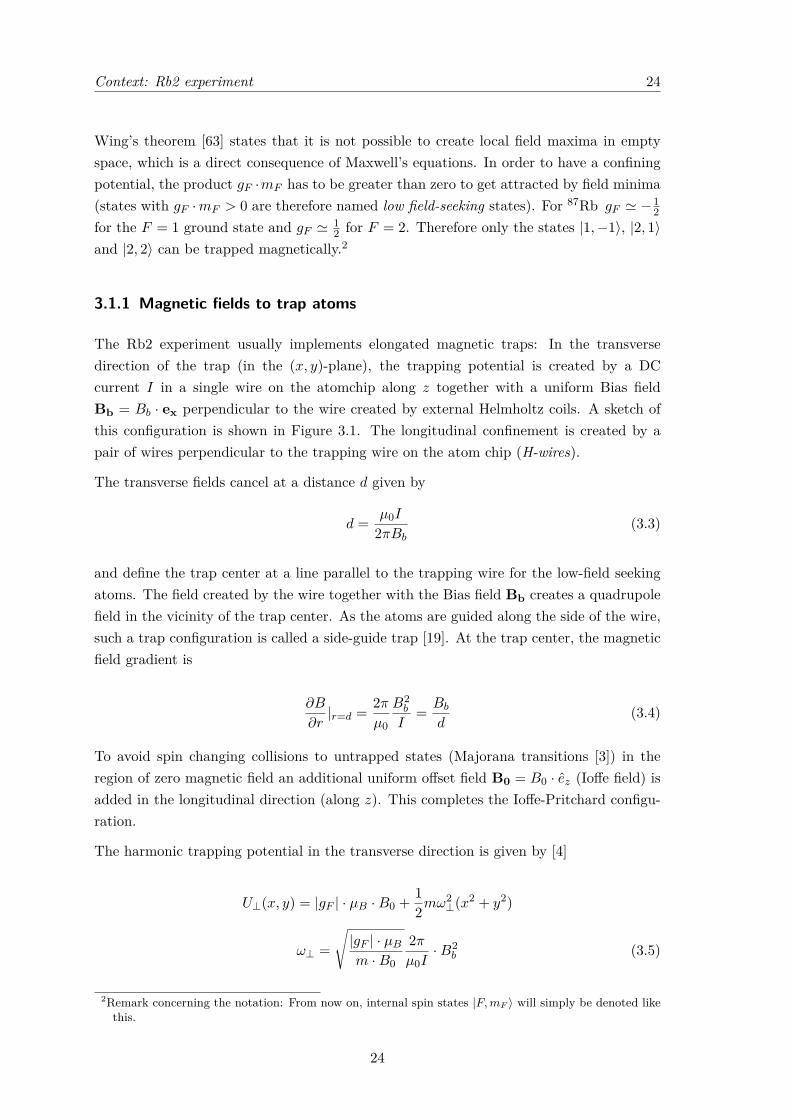


![Bose-Einstein Condensation with High Atom Number in a Deep ... · Bose-Einstein condensation was predicted in 1925 [Bose, 1924, Einstein, 1925], at the time when quantum mechanics](https://static.documents.pub/doc/80x56/5f0235fc7e708231d4031fe6/bose-einstein-condensation-with-high-atom-number-in-a-deep-bose-einstein-condensation.jpg)

![AVALANCHES IN A BOSE-EINSTEIN CONDENSATE · 1.4.1.1 BOSE-EINSTEIN CONDENSATION The realization of Bose-Einstein condensation in dilute gases in 1995 [1] was a milestone in the rapidly](https://static.documents.pub/doc/80x56/5f0235fc7e708231d4031fe8/avalanches-in-a-bose-einstein-condensate-1411-bose-einstein-condensation-the.jpg)


