TRACE OPTIMIZATION AND EIGENPROBLEMS IN DIMENSION REDUCTION METHODS E. KOKIOPOULOU * , J. CHEN † , AND Y. SAAD † Abstract. This paper gives an overview of the eigenvalue problems encountered in areas of data mining that are related to dimension reduction. Given some input high-dimensional data, the goal of dimension reduction is to map them to a low- dimensional space such that certain properties of the initial data are preserved. Optimizing the above properties among the reduced data can be typically posed as a trace optimization problem that leads to an eigenvalue problem. There is a rich variety of such problems and the goal of this paper is to unravel relations between them as well as to discuss effective solution techniques. First, we make a distinction between projective methods that determine an explicit linear projection from the high-dimensional space to the low-dimensional space, and nonlinear methods where the mapping between the two is nonlinear and implicit. Then, we show that all of the eigenvalue problems solved in the context of explicit projections can be viewed as the projected analogues of the so-called nonlinear or implicit projections. We also discuss kernels as a means of unifying both types of methods and revisit some of the equivalences between methods established in this way. Finally, we provide some illustrative examples to showcase the behavior and the particular characteristics of the various dimension reduction methods on real world data sets. Key words. Linear Dimension Reduction, Nonlinear Dimension Reduction, Principal Component Analysis, Projection methods, Locally Linear Embedding (LLE), Kernel methods, Locality Preserving Projections (LPP), Laplacean Eigenmaps. 1. Introduction. The term ‘data mining’ refers to a broad discipline which includes such diverse areas as machine learning, data analysis, information retrieval, pattern recognition, and web-searching, to list just a few. The widespread use of linear algebra techniques in many sub-areas of data mining is remarkable. A prototypical area of data mining where numerical linear algebra techniques play a crucial role is that of dimension reduction which is the focus of this study. Dimension reduction is ubiquitous in applications ranging from pattern recognition and learning [50] to the unrelated fields of graph drawing [26, 32], materials research [13, 11], and magnetism [42]. Given a set of high-dimensional data, the goal of dimension reduction is to map the data to a low-dimensional space. Specifically, we are given a data matrix X =[x 1 ,...,x n ] ∈ R m×n , (1.1) for which we wish to find a low-dimensional analogue Y =[y 1 ,...,y n ] ∈ R d×n , (1.2) with d ≪ m, which is a faithful representation of X in some sense. As will be seen, many of the dimension reduction techniques lead to optimization problems which typically involve a trace. This in turn leads to eigenvalue problems [38]. It may be helpful to define some terms used in data mining. Among the many problems which arise in data mining, two are of primary importance. One is ‘unsupervised clustering’, which is the task of finding subsets of the data such that items from the same subset are most similar and items from distinct subsets are most dissimilar. The second is classification (supervised learning), whereby we are given a set of distinct sets that are labeled (e.g. samples of handwritten digits labeled from 0 to 9) and when a new sample is presented to us we must determine to which of the sets is it most likely to belong. For the example of * Seminar for Applied Mathematics, ETH, HG G J49, R¨ amistrasse 101, 8092 Z¨ urich, Switzerland. Email: [email protected]† Department of Computer Science and Engineering; University of Minnesota; Minneapolis, MN 55455. Email: (jchen, saad)@cs.umn.edu. Work supported by NSF under grant DMS-0810938 and by the Minnesota Supercomputer Institute. 1
Transcript
TRACE OPTIMIZATION AND EIGENPROBLEMS IN DIMENSION
REDUCTION METHODS
E. KOKIOPOULOU∗, J. CHEN† , AND Y. SAAD†
Abstract. This paper gives an overview of the eigenvalue problems encountered in areas of data mining that are relatedto dimension reduction. Given some input high-dimensional data, the goal of dimension reduction is to map them to a low-dimensional space such that certain properties of the initial data are preserved. Optimizing the above properties among thereduced data can be typically posed as a trace optimization problem that leads to an eigenvalue problem. There is a richvariety of such problems and the goal of this paper is to unravel relations between them as well as to discuss effective solutiontechniques. First, we make a distinction between projective methods that determine an explicit linear projection from thehigh-dimensional space to the low-dimensional space, and nonlinear methods where the mapping between the two is nonlinearand implicit. Then, we show that all of the eigenvalue problems solved in the context of explicit projections can be viewedas the projected analogues of the so-called nonlinear or implicit projections. We also discuss kernels as a means of unifyingboth types of methods and revisit some of the equivalences between methods established in this way. Finally, we provide someillustrative examples to showcase the behavior and the particular characteristics of the various dimension reduction methodson real world data sets.
Key words. Linear Dimension Reduction, Nonlinear Dimension Reduction, Principal Component Analysis, Projectionmethods, Locally Linear Embedding (LLE), Kernel methods, Locality Preserving Projections (LPP), Laplacean Eigenmaps.
1. Introduction. The term ‘data mining’ refers to a broad discipline which includes suchdiverse areas as machine learning, data analysis, information retrieval, pattern recognition,and web-searching, to list just a few. The widespread use of linear algebra techniques in manysub-areas of data mining is remarkable. A prototypical area of data mining where numericallinear algebra techniques play a crucial role is that of dimension reduction which is thefocus of this study. Dimension reduction is ubiquitous in applications ranging from patternrecognition and learning [50] to the unrelated fields of graph drawing [26, 32], materialsresearch [13, 11], and magnetism [42]. Given a set of high-dimensional data, the goal ofdimension reduction is to map the data to a low-dimensional space. Specifically, we aregiven a data matrix
X = [x1, . . . , xn] ∈ Rm×n, (1.1)
for which we wish to find a low-dimensional analogue
Y = [y1, . . . , yn] ∈ Rd×n, (1.2)
with d ≪ m, which is a faithful representation of X in some sense. As will be seen, many ofthe dimension reduction techniques lead to optimization problems which typically involve atrace. This in turn leads to eigenvalue problems [38].
It may be helpful to define some terms used in data mining. Among the many problemswhich arise in data mining, two are of primary importance. One is ‘unsupervised clustering’,which is the task of finding subsets of the data such that items from the same subset aremost similar and items from distinct subsets are most dissimilar. The second is classification(supervised learning), whereby we are given a set of distinct sets that are labeled (e.g.samples of handwritten digits labeled from 0 to 9) and when a new sample is presented tous we must determine to which of the sets is it most likely to belong. For the example of
∗Seminar for Applied Mathematics, ETH, HG G J49, Ramistrasse 101, 8092 Zurich, Switzerland. Email:[email protected]
†Department of Computer Science and Engineering; University of Minnesota; Minneapolis, MN 55455. Email: (jchen,
saad)@cs.umn.edu. Work supported by NSF under grant DMS-0810938 and by the Minnesota Supercomputer Institute.
1
handwritten digits this is the problem of recognizing a digit given many labeled samples ofalready deciphered digits available in a given data set. In order to perform these tasks it iscommon to first process the given datasets (e.g. the database of handwritten digits) in orderto reduce its dimension, i.e., to find a dataset of much lower dimension than the original onebut which preserves its main features. What is often misunderstood is that this dimensionreduction is not done for the sole purpose of reducing cost but mainly for reducing the effectof noise and extracting the main features of the data. For this reason the term “featureextraction” is sometimes used in the literature instead of dimension reduction.
There have been two types of methods proposed for dimension reduction. The first classof methods can be termed “projective”. This includes all linear methods whereby the datamatrix is explicitly transformed into a low-dimensional version. Then these projective meth-ods find an explicit linear transformation to perform the reduction, i.e., they find a m × dmatrix V and express the reduced dimension data as Y = V T X. This class of methodsincludes the standard Principal Component Analysis (PCA), the Locality Preserving Pro-jection (LPP) [22], the Orthogonal Neighborhood Preserving Projections, (ONPP) [24] andother variants of these. A second class of methods that do not rely on explicit projectionsand are inherently nonlinear [27], find directly the low dimensional data matrix Y , by simplyimposing that certain locality or affinity between near-by points be preserved. Furthermore,both types of dimension reduction methods can be extended to their supervised versions,where each data point is associated with a class label and the class labels are taken intoaccount when performing the reduction step.
The goal of this paper is to try to unravel some of the relationships between thesedimension reduction methods, their supervised counterparts and the optimization problemsthat they rely upon. The paper will not describe the details of the various applications.Instead these will be summarized and expressed in simple mathematical terms with thegoal of showing the objective function that is optimized in each case. In addition, twomain observations will be made in this paper. The first is about a distinction between theprojective methods and the nonlinear ones. Specifically, the eigenvalue problem solved inthe linear case consists of applying a projection technique, i.e., a Rayleigh-Ritz projectionmethod, as it leads to the solution of an eigenvalue problem in the space spanned by thecolumns of the data matrix XT . The second is that these two families of methods can bebrought together thanks to the use of kernels. These observations will strengthen a fewsimilar observations made in a few earlier papers, e.g., [24, 21, 55]. The observation thatkernels can help unify dimension reduction has been made before. Ham et al [21] notethat several of the known standard methods (LLE [34], Isomap [46], Laplacean eigenmaps[4, 5] can be regarded as some form of Kernel PCA. In [24], it was observed that linear andnonlinear projection methods are in fact equivalent, in the sense that one can define onefrom the other with the help of kernels.
Producing a set Y in the form (1.2) that is an accurate representation of the set X in(1.1), with d ≪ m, can be achieved in different ways by selecting the type of the reduceddata Y as well as the desirable properties to be preserved. By type we mean whether werequire that Y be simply a low-rank representation of X, or a data set in a vector space withfewer dimensions. Examples of properties to be preserved may include the global geometry,neighborhood information such as local neighborhoods [5, 34] and local tangent space [60],distances between data points [46, 54], or angles formed by adjacent line segments [43]. The
2
mapping from X to Y may be implicit (i.e., not known via an explicit function) or explicit.Nonlinear (i.e., implicit) methods make no assumptions about the mapping and they onlycompute for each xi its corresponding yi in the reduced space. On the other hand, linearmethods compute an explicit linear mapping between the two.
The rest of this paper is organized as follows. Section 2 summarizes a few well-knownresults of linear algebra that will be exploited repeatedly in the paper. Then, Sections 3 and 4provide a brief overview of nonlinear and linear methods respectively for dimension reduction.Section 5 discusses dimension reduction in supervised settings, where the class labels of thedata are taken into account. Section 6 provides an analysis of relations between the differentmethods as well as connections to methods from different areas, such as spectral clusteringand projection techniques for eigenvalue problems. Kernelized versions of different lineardimension reduction methods are discussed in Section 7, along with various relationshipswith their nonlinear counterparts. Finally, Section 8 provides illustrative examples for datavisualization and classification of handwritten digits and faces, and the paper ends with aconclusion in Section 10.
2. Preliminaries. First, given a symmetric matrix A, of dimension n×n and an arbitraryunitary matrix V of dimension n × d then the trace of V T AV is maximized when V is anorthogonal basis of the eigenspace associated with the (algebraically) largest eigenvalues.In particular, it is achieved for the eigenbasis itself: if eigenvalues are labeled decreasinglyand u1, · · · , ud are eigenvectors associated with the first d eigenvalues λ1, · · · , λd, and U =[u1, · · · , ud], with UT U = I, then,
max8
<
:
V ∈ Rn×d
V T V = I
Tr[V T AV
]= Tr
[UT AU
]= λ1 + · · · + λd. (2.1)
While this result is seldom explicitly stated on its own in standard textbooks, it is an imme-diate consequence of the Courant-Fisher characterization, see, e.g., [33, 35]. It is importantto note that the optimal V is far from being unique. In fact, any V which is an orthonormalbasis of the eigenspace associated with the first d eigenvalues will be optimal. In other words,what matters is the subspace rather than a particular orthonormal basis for it.
The main point is that to maximize the trace in (2.1), one needs to solve a standardeigenvalue problem. In many instances, we need to maximize Tr [V T AV ] subject to a newnormalization constraint for V , one that requires that V be B-orthogonal, i.e., V T BV =I. Assuming that A is symmetric and B positive definite, we know that there are n realeigenvalues for the generalized problem Au = λBu, with B-orthogonal eigenvectors. Ifthese eigenvalues are labeled decreasingly, and if U = [u1, · · · , ud] is the set of eigenvectorsassociated with the first d eigenvalues, with UT BU = I, then we have
max8
<
:
V ∈ Rn×d
V T BV = I
Tr[V T AV
]= Tr
[UT AU
]= λ1 + · · · + λd. (2.2)
In reality, Problem (2.2) often arises as a simplification of an objective function that is3
more difficult to maximize, namely:
max8
<
:
V ∈ Rn×d
V T CV = I
Tr[V T AV
]
Tr [V T BV ]. (2.3)
Here B and C are assumed to be symmetric and positive definite for simplicity. The matrixC defines the desired orthogonality and in the simplest case it is just the identity matrix. Theoriginal version shown above has resurfaced in recent years, see, e.g., [19, 49, 56, 59] amongothers. Though we will not give the above problem as much attention as the more standardproblem (2.2), it is important to give an idea on the way it is commonly solved. There isno loss of generality in assuming that C is the identity. Since B is assumed to be positivedefinite1, it is not difficult to see that there is a maximum µ that is reached for a certain (non-unique) orthogonal matrix, which we will denote by U . Then, Tr [V T AV ]−µ Tr [V T BV ] ≤ 0for any orthogonal V . This means that for this µ we have Tr [V T (A − µB)V ] ≤ 0 for anyorthogonal V , and also Tr [UT (A − µB)U ] = 0. Therefore we have the following necessarycondition for the pair µ, U to be optimal:
maxV T V =I
Tr [V T (A − µB)V ] = Tr [UT (A − µB)U ] = 0. (2.4)
According to (2.1), the maximum trace of V T (A − µB)V is simply the sum of the largest deigenvalues of A − µB and U is the set of corresponding eigenvectors. If µ maximizes thetrace ratio (2.3) (with C = I), then the sum of the largest d eigenvalues of the pencil A−µBequals zero, and the corresponding eigenvectors form the desired optimal solution of (2.3).
When B is positive definite, it can be seen that the function
f(θ) = maxV T V =I
Tr [V T (A − θB)V ]
is a decreasing function of θ. For θ = 0 we have f(θ) > 0. For θ > λmax(A,B) wehave f(θ) < 0, where λmax(A,B) is the largest generalized eigenvalue of the pencil (A,B).Finding the optimal solution will involve a search for the (unique) root of f(θ). In [49] and[19] algorithms were proposed to solve (2.3) by computing this root and by exploiting theabove relations. No matter what method is used it appears clear that it will be far moreexpensive to solve (2.3) than (2.2), because the search for the root µ will typically involvesolving several eigenvalue problems instead of just one.
3. Nonlinear dimension reduction. We start with an overview of nonlinear methods. Inwhat follows, we discuss LLE and Laplacean Eigenmaps, which are the most representativenonlinear methods for dimensionality reduction. These methods begin with the constructionof a weighted graph which captures some information on the local neighborhood structureof the data. In the sequel, we refer to this graph as the “affinity graph”. Specifically, theaffinity (or adjacency) graph is a graph G = (V , E) whose nodes V are the data samples. Theedges of this graph can be defined for example by taking a certain nearness measure andincluding all points within a radius ǫ of a given node, to its adjacency list. Alternatively,
1We can relax the assumptions: B can be positive semidefinite, but for the problem to be well-posed its null space must beof dimension less than d. Also if A is positive semidefinite, we must assume that Null(A) ∩ Null(B) = ∅.
4
one can include those k nodes that are the nearest neighbors to xi. In the latter case it iscalled the k-NN graph. It is typical to assign weights wij on the edges eij ∈ E of the affinitygraph. The affinity graph along with these weights then defines a matrix W whose entriesare the weights wij’s that are nonzero only for adjacent nodes in the graph.
3.1. LLE. In Locally Linear Embedding (LLE), the construction of the affinity graph isbased on the assumption that the points lie on some high-dimensional manifold, so eachpoint is approximately expressed as a linear combination of a few neighbors, see [34, 37].Thus, the affinity matrix is built by computing optimal weights which will relate a givenpoint to its neighbors in some locally optimal way. The reconstruction error for sample i canbe measured by
∥∥∥∥∥xi −
∑
j
wijxj
∥∥∥∥∥
2
2
. (3.1)
The weights wij represent the linear coefficients for (approximately) reconstructing the sam-ple xi from its neighbors {xj}, with wij = 0, if xj is not one of the k nearest neighbors of xi.We can set wii ≡ 0, for all i. The coefficients are scaled so that their sum is unity, i.e.,
∑
j
wij = 1. (3.2)
Determining the wij’s for a given point xi is a local calculation, in the sense that it onlyinvolves xi and its nearest neighbors. As a result computing the weights will be fairlyinexpensive; an explicit solution can be extracted by solving a small linear system whichinvolves a ‘local’ Grammian matrix, for details see [34, 37]. After this phase is completedwe have available a matrix W which is such that each column xi of the data set is wellrepresented by the linear combination
∑
j wijxj. In other words, X ≈ XW T , i.e., XT is aset of approximate left null vectors of I − W .
The procedure then seeks d-dimensional vectors yi, i = 1, . . . , n so that the same relationis satisfied between the matrix W and the yi’s. This is achieved by minimizing the objectivefunction
FLLE(Y ) =∑
i
‖yi −∑
j
wijyj‖22. (3.3)
LLE imposes two constraints to this optimization problem: i) the mapped coordinates mustbe centered at the origin and ii) the embedded vectors must have unit covariance:
∑
i
yi = 0; and1
n
∑
i
yiyTi = I . (3.4)
The objective function (3.3) is minimized with these constraints on Y .We can rewrite (3.3) as a trace by noting that FLLE(Y ) = ‖Y − Y W T‖2
F , and this leadsto:
FLLE(Y ) = Tr[Y (I − W T )(I − W )Y T
]. (3.5)
5
Therefore the new optimization problem to solve is2
min8
<
:
Y ∈ Rd×n
Y Y T = I
Tr[Y (I − W T )(I − W )Y T
]. (3.6)
The solution of the problem is obtained from the set of eigenvectors associated with the dsmallest eigenvalues of M ≡ (I − W T )(I − W ):
(I − W T )(I − W )ui = λiui; Y = [u2, · · · , ud+1]T . (3.7)
Note that the eigenvector associated with the eigenvalue zero is discarded and that thematrix Y is simply the set of bottom eigenvectors of (I − W T )(I − W ) associated with the2nd to (d + 1)-th eigenvalues. We will often refer to the matrix M = (I − W T )(I − W ) asthe LLE matrix.
3.2. Laplacean Eigenmaps. The Laplacean Eigenmaps technique is rather similar to LLE.It uses different weights to represent locality and a slightly different objective function. Twocommon choices are weights of the heat kernel wij = exp(−‖xi −xj‖
22/t) or constant weights
(wij = 1 if i and j are adjacent, wij = 0 otherwise). It is important to note that the choiceof the parameter t is crucial to the performance of this method. The name heat ‘kernel’ isself explaining, since the matrix [wij] happens to be positive semi-definite.
Once this graph is available, a Laplacean matrix of the graph is constructed, by settinga diagonal matrix D with diagonal entries dii =
∑
j wij. The matrix
L ≡ D − W
is the Laplacean of the weighted graph defined above. Note that the row-sums of the matrixL are zero by the definition of D, so L1 = 0, and therefore L is singular. The problem inLaplacean Eigenmaps is then to minimize
FEM(Y ) =n∑
i,j=1
wij‖yi − yj‖22 (3.8)
subject to an orthogonality constraint that uses the matrix D for scaling:
Y DY T = I .
The rationale for this approach is to put a penalty for mapping nearest neighbor nodes in theoriginal graph to distant points in the low-dimensional data.
Compare (3.8) and (3.3). The difference between the two is subtle and one might ask if(3.8) can also be converted into a trace optimization problem similar to (3.6). As it turnsout FEM can be written as a trace that will put the method quite close to LLE in spirit:
FEM(Y ) = 2Tr [Y (D − W )Y T ]. (3.9)
Therefore the new optimization problem to solve is
min8
<
:
Y ∈ Rd×n
Y D Y T = I
Tr[Y (D − W )Y T
]. (3.10)
2The final yi’s are obtained by translating and scaling each column of Y .
6
The solution Y to this optimization problem can be obtained from the eigenvectors associatedwith the d smallest eigenvalues of the generalized eigenvalue problem
(D − W )ui = λiDui ; Y = [u2, · · · , ud+1]T . (3.11)
One can also solve a standard eigenvalue problem by making a small change of variablesand this is useful to better see links with other methods. Indeed, it would be useful tostandardize the constraint Y DY T so that the diagonal scaling does not appear. For this weset Y = Y D1/2 and W = D−1/2WD−1/2, and this simplifies (3.10) into:
min8
<
:
Y ∈ Rd×n
Y Y T = I
Tr[
Y (I − W )Y T]
. (3.12)
In this case, (3.11) yields:
(I − W )ui = λiui ; Y = [u2, · · · , ud+1]T D1/2 . (3.13)
The quantity L = I − W = D−1/2LD−1/2 is called the normalized Laplacean.
4. Linear dimension reduction. The methods in the previous section do not provide an ex-plicit function that maps a vector x into its low-dimensional representation y in d-dimensionalspace. This mapping is only known for each of the vectors xi of the data set X. For each xi
we know how to associate a low-dimensional item yi. In some applications it is importantto be able to find the mapping y for an arbitrary, ‘out-of-sample’ vector x. The methodsdiscussed in this section have been developed in part to address this issue. They are basedon using an explicit (linear) mapping defined by a matrix V ∈ R
m×d. These projectivetechniques replace the original data X by a matrix of the form
Y = V T X, where V ∈ Rm×d. (4.1)
Once the matrix V has been learned, each vector xi can be projected to the reduced spaceby simply computing yi = V T xi. If V is a unitary matrix, then Y represents the orthogonalprojection of X into the V -space.
4.1. PCA. The best known technique in this category is Principal Component Analysis(PCA). PCA computes an orthonormal matrix V such that the variance of the projectedvectors is maximized, i.e, V is the maximizer of
maxV ∈ R
m×d
V T V = I
n∑
i=1
∥∥∥∥∥yi −
1
n
n∑
j=1
yj
∥∥∥∥∥
2
2
, yi = V T xi. (4.2)
Recalling that 1 denotes the vector of all ones, the objective function in (4.2) becomes
FPCA(Y ) =n∑
i=1
∥∥∥∥∥yi −
1
n
n∑
j=1
yj
∥∥∥∥∥
2
2
= Tr
[
V T X(I −1
n11
T )XT V
]
.
7
In the end, the above optimization can be restated as
max8
<
:
V ∈ Rm×d
V T V = I
Tr
[
V T X(I −1
n11
T )XT V
]
. (4.3)
In the sequel we will denote by X the matrix X(I − 1n11
T ) which is simply the matrix withcentered data, i.e., each column is xi = xi −µ where µ is the mean of X, µ =
∑xi/n. Since
the matrix in (4.3) can be written V T XXT V , so (4.3) becomes
max8
<
:
V ∈ Rm×d
V T V = I
Tr[V T XXT V
]. (4.4)
The orthogonal matrix V which maximizes the trace in (4.4) is simply the set of left singularvectors of X, associated with the largest d singular values,
[XX]T vi = λivi. (4.5)
The matrix V = [v1, · · · , vd] is used for projecting the data, so Y = V T X. If X = UΣZT isthe SVD of X, the solution to the above optimization problem is V = Ud, the matrix of thefirst d left singular vectors of X, so, denoting by Σd the top left d× d block of Σ, and Zd thematrix of the first d columns of Z, we obtain
Y = UTd X = ΣdZ
Td . (4.6)
As it turns out, maximizing the variance on the projected space is equivalent to mini-mizing the projection error
‖X − V V T X‖2F = ‖X − V Y ‖2
F .
This is because a little calculation will show that
‖X − V Y ‖2F = Tr [(X − V Y )T (X − V Y )] = Tr [XT X] − Tr [V T XXT V ].
The matrix V V T is an orthogonal projector onto the span of V . The points V yi ∈ Rm are
sometimes referred to as reconstructed points. PCA minimizes the sum of the squares of thedistance between any point in the data set and its reconstruction, i.e., its projection.
4.2. MDS and ISOMAP3. In metric Multi-Dimensional Scaling (metric MDS) the prob-lem posed is to project data in such a way that distances ‖yi−yj‖2 between projected pointsare closest to the original distances ‖xi − xj‖2. Instead of solving the problem in this form,MDS uses a criterion based on inner products.
It is now assumed that the data is centered at zero so we replace X by X. An importantresult used is that one can recover distances from inner products and vice-versa. The matrixof inner products, i.e., the Grammian of X, defined by
G = [〈xi, xj〉]i,j=1,··· ,n (4.7)
3These methods are essentially not linear methods; however, they are very closely related to PCA and better be presentedin this section.
8
determines completely the distances, since ‖xi − xj‖2 = gii + gjj − 2gij. The reverse can also
be done, i.e., one can determine the inner products from distances by ‘inverting’ the aboverelations. Indeed, under the assumption that the data is centered at zero, it can be shownthat [47]
gij =1
2
[
1
n
∑
k
(sik + sjk) − sij −1
n2
∑
k,l
skl
]
,
where sij = ‖xi − xj‖2. In the matrix form, it is
G = −1
2[I −
1
n11
T ]S[I −1
n11
T ] ; S = [sij]i,j=1,...,n.
As a result of the above equality, in order to find a d-dimensional projection which preservesinter-distances as best possible, we need to find a d× n matrix Y whose Grammian Y T Y isclose to G, the Grammian of X, i.e., we need to find the solution of
minY ∈ Rd×n
‖G − Y T Y ‖2F . (4.8)
Let G = ZΛZT be the eigenvalue decomposition of G, where it is assumed that the eigen-
values are labeled from largest to smallest. Then the solution to (4.8) is Y = Λ1/2d ZT
d whereZd consists of the first d columns of Z, Λd is the d× d upper left block of Λ. Note that withrespect to the SVD of X this is equal to ΣdZ
Td , which is identical with the result obtained
with PCA, see equation (4.6). So metric MDS gives the same exact result as PCA. Howeverit arrives at this result using a different path. PCA uses the covariance matrix, while MDSuses the Gram matrix. From a computational cost point of view, there is no real difference ifthe calculation is based on the SVD of X. We should note that the solution to (4.8) is unique
only up to unitary transformations. This is because a transformation such as Y = QY of Y ,where Q is unitary, will not change distances between y-points.
Finally, we mention in passing that the technique of ISOMAP [46] essentially performsthe same steps as MDS, except that the Grammian G = XT X is replaced by a pseudo-Grammian G obtained from geodesic distances between the points xi:
G = −1
2[I −
1
n11
T ]S[I −1
n11
T ] ; S = [sij]i,j=1,...,n,
where sij is the squared shortest graph distance between xi and xj.
4.3. LPP. The Locality Preserving Projections (LPP) [22] is a graph-based projectivetechnique. It projects the data so as to preserve a certain affinity graph constructed fromthe data. LPP defines the projected points in the form yi = V T xi by putting a penaltyfor mapping nearest neighbor nodes in the original graph to distant points in the projecteddata. Therefore, the objective function to be minimized is identical with that of LaplaceanEigenmaps,
FLPP (Y ) =n∑
i,j=1
wij‖yi − yj‖22 .
9
The matrix V , which is the actual unknown, is implicitly represented in the above function,through the dependence of the yi’s on V . Writing Y = V T X, we reach the optimizationproblem,
min8
<
:
V ∈ Rm×d
V T (XDXT ) V = I
Tr[V T X(D − W )XT V
](4.9)
whose solution can be computed from the generalized eigenvalue problem
X(D − W )XT vi = λiXDXT vi. (4.10)
Similarly to Eigenmaps, the smallest d eigenvalues and eigenvectors must be computed.It is simpler to deal with the ‘normalized’ case of LPP, by scaling the set Y as before in
the case of Laplacean Eigenmaps (see eq. (3.12)). We define Y = Y D1/2 = V T XD1/2. So, if
X = XD1/2, we have Y = V T X, and the above problem then becomes
min8
<
:
V ∈ Rm×d
V T (XXT ) V = I
Tr[
V T X(I − W )XT V]
(4.11)
where W is the same matrix as in (3.12). The eigenvalue problem to solve is now
X(I − W )XT vi = λiXXT vi. (4.12)
The projected data yi is defined by yi = V T xi for each i, where V = [v1, · · · , vd].
4.4. ONPP. Orthogonal Neighborhood Preserving Projection (ONPP) [24, 25] seeks anorthogonal mapping of a given data set so as to best preserve the same affinity graph asLLE. In other words, ONPP is an orthogonal projection version of LLE. The projectionmatrix V in ONPP is determined by minimizing the same objective function as in (3.5),with the additional constraint that Y is of the form Y = V T X and the columns of V beorthonormal, i.e. V T V = I. The optimization problem becomes
min8
<
:
V ∈ Rm×d
V T V = I
Tr[V T X(I − W T )(I − W )XT V
]. (4.13)
Its solution is the basis of the eigenvectors associated with the d smallest eigenvalues of thematrix M ≡ X(I − W T )(I − W )XT = XMXT .
X(I − W T )(I − W )XT ui = λui. (4.14)
Then the projector V is [u1, u2, · · · , ud] and results in the projected data Y = V T X.The assumptions that were made when defining the weights wij in Section 3.1 imply that
the n× n matrix I −W is singular due to eq. (3.2). In the case when m > n the matrix M ,which is of size m × m, is at most of rank n and it is therefore singular. In the case whenm ≤ n, M is not necessarily singular but it is observed in practice that ignoring the smallesteigenvalue is helpful [25].
10
4.5. Other variations on the locality preserving theme. A few possible variations of themethods discussed above can be developed. As was seen ONPP is one such variation whichadapts the LLE affinity graph and seeks a projected data which preserves this graph just asin LLE. Another very simple option is to solve the same optimization problem as ONPP butrequire the same orthogonality of the projected data as LLE, namely: Y Y T = I. This yieldsthe constraint V T XXT V = I instead of the V T V = I required in ONPP. In [24] we calledthis Neighborhood Preserving Projections (NPP). The resulting new optimization problem isthe following modification of (4.13)
min8
<
:
V ∈ Rm×d
V T XXT V = I
Tr[V T X(I − W T )(I − W )XT V
]. (4.15)
and the new solution is
X(I − W T )(I − W )XT ui = λ(XXT )ui. (4.16)
As before, V = [u1, · · · , ud] and yi = V T xi, i = 1, · · · , n.Another variation goes in the other direction by using the objective function of LPP
(using graph Laplaceans) and requiring the data to be orthogonally projected:
min8
<
:
V ∈ Rm×d
V T V = I
Tr[V T X(D − W )XT V
]. (4.17)
This was referred to as Orthogonal Locality Preserving Projections (OLPP), in [24]. Note inpassing that a different technique was developed in [10] and named Orthogonal Laplaceanfaces, which is also sometimes referred to as OLPP. We will not refer to this method in thispaper and there is therefore no confusion.
5. Supervised dimension reduction. The problem of classification can be described asfollows. We are given a data set consisting of c known subsets (classes or clusters) which arelabeled from 1 to c. When a new item is presented to us, we need to determine to which ofthe classes (clusters) it is the most related in some sense. When the class labels of the dataset are taken into account during dimension reduction, the process is called supervised (andunsupervised in the opposite case). It has been observed in general that supervised methodsperform better in many classification tasks relative to the unsupervised ones. In what follows,we first describe supervised versions of the above graph-based methods and then we discussLinear Discriminant Analysis (LDA), which is one of the most popular supervised techniquesfor linear dimension reduction.
5.1. Supervised graph-based methods. As discussed so far, the above methods do notmake use of class labels. It is possible to develop supervised versions of the above methodsby taking the class labels into account. Assume that we have c classes and that the dataare organized, without loss of generality, as X1, · · · , Xc with Xi ∈ R
m×ni , where ni denotesthe number of samples that belong to the ith class. In other words, assume that the datasamples are ordered according to their class membership.
In supervised methods the class labels are used to build the graph. The main idea is tobuild the graph in a discriminant way in order to reflect the categorization of the data into
11
different classes. One simple approach is to impose that an edge eij = (xi, xj) exists if andonly if xi and xj belong to the same class. In other words, we make adjacent those nodesthat belong to the same class. For instance, preserving localities in such a supervised graph,will result in samples from the same class being projected close-by in the reduced space.
Consider now the structure of the induced adjacency matrix H. Observe that the datagraph G consists of c cliques, since the adjacency relationship between two nodes reflectstheir class membership. Let 1nj
denote the vector of all ones, with length nj, and Hj =1nj
1nj1
Tnj
∈ Rnj×nj be the block corresponding to the jth class. The n× n adjacency matrix
H will be of the following form
H = diag[H1, H2, · · · , Hc]. (5.1)
Thus, the (1,1) diagonal block is of size n1 × n1 and has the constant entries 1/n1, the (2,2)diagonal block is of size n2×n2 and has the constant entries 1/n2, and so on. Using the abovesupervised graph in the graph-based dimension reduction methods yields their supervisedversions.
5.2. LDA. The principle used in Linear Discriminant Analysis (LDA) is to projectthe original data linearly in such a way that the low-dimensional data is best separated.Fisher’s Linear Discriminant Analysis, see, e.g., Webb [50], seeks to project the data in low-dimensional space so as to maximize the ratio of the “between scatter” measure over “withinscatter” measure of the classes, which are defined next. Let µ be the mean of all the dataset, and µ(k) be the mean of the k-th class, which is of size nk, and define the two matrices
SB =c∑
k=1
nk(µ(k) − µ)(µ(k) − µ)T , (5.2)
SW =c∑
k=1
∑
xi ∈Xk
(xi − µ(k))(xi − µ(k))T . (5.3)
If we project the set on a one-dimensional space spanned by a given vector a, then thequantity
aT SBa =c∑
i=1
nk|aT (µ(k) − µ)|2
represents a weighted sum of (squared) distances of the projection of the centroids of eachset from the mean µ. At the same time, the quantity
aT SW a =c∑
k=1
∑
xi ∈ Xk
|aT (xi − µ(k))|2
is the sum of the variances of each the projected sets.LDA projects the data so as to maximize the ratio of these two numbers:
maxa
aT SBa
aT SW a. (5.4)
12
This optimal a is known to be the eigenvector associated with the largest eigenvalue of thepair (SB, SW ). If we call ST the total covariance matrix
ST =∑
xi ∈ X
(xi − µ)(xi − µ)T , (5.5)
then,
ST = SW + SB. (5.6)
Therefore, (5.4) is equivalent to
maxa
aT SBa
aT ST a, (5.7)
or
mina
aT SW a
aT ST a, (5.8)
where an optimal a is known to be the eigenvector associated with the largest eigenvalue ofthe pair (SB, ST ), or the smallest eigenvalue of the pair (SW , ST ).
The above one-dimensional projection is generalized to ones on d-dimensional spaces, i.e.,modify the objective function such that the vector a is replaced by a matrix V . A traditionalway is to minimize the trace of V T SBV while requiring the columns of the solution matrixV to be SW -orthogonal, i.e., imposing the condition V T SW V = I. The optimum is achievedfor the set of eigenvectors of the generalized eigenvalue problem
SBui = λiSW ui ,
associated with the largest d eigenvalues. Incidentally, the above problem can also be for-mulated as a generalized singular value problem (see e.g., [23]). Another approach [49] caststhe problem as minimizing the ratio of the two traces:
max8
<
:
V ∈ Rn×d
V T V = I
Tr[V T SBV
]
Tr [V T SW V ].
Approaches for solving this problem were briefly discussed in Section 2.Note that with simple algebraic manipulations, the matrices SB, SW and ST can be
expressed in terms of the data matrix X:
SB = XHXT ,
SW = X(I − H)XT ,
ST = XXT .
The matrix SB has rank at most c because each of the blocks in H has rank one and thereforethe matrix H itself has rank c. Because the matrix I − H is an orthogonal projector, itsrange is the null-space of H which has dimension n − c. Thus, I − H which plays the roleof a Laplacean, has rank at most n − c. The corresponding eigenvalue problem to solve for(5.8) is
X(I − H)XT ui = λi(XXT )ui (5.9)
13
6. Connections between dimension reduction methods. This section establishes connec-tions between the various methods discussed in previous sections.
6.1. Relation between the LLE matrix and the Laplacan matrix. A comparison between(3.6) and (3.12) shows that the two are quite similar. The only difference is in the matrix
inside the bracketed term. In one case it is of the form Y (I − W )Y T where I − W is thenormalized graph Laplacean, and in the other it is of the form Y (I −W T )(I −W )Y T whereW is an affinity matrix. Can one just interpret the LLE matrix (I − W T )(I − W ) as aLaplacean matrix? A Laplacean matrix L associated with a graph is a a symmetric matrixwhose off-diagonal entries are non-positive, and whose row-sums are zero (or equivalently,the diagonal entries are the negative sums of the off-diagonal entries). In other words, lij ≤ 0for i 6= 0, lii = −
∑
j lij. The LLE matrix M = (I−W )T (I−W ) satisfies the second property
(zero row sum) but not the first (nonpositive off-diagonals) in general.Proposition 6.1. The symmetric matrix M = (I − W )T (I − W ) has zero row (and
column) sums. In addition, denoting by w:j the j-th column of W ,
Proof. Since (I − W ) has row sums equal to zero, then (I − W )1 = 0 and thereforeM1 = (I − W T )(I − W )1 = 0, which shows that the row sums of M are zero. Since M issymmetric, its column-sums are also zero. Since M = I −W −W T + W TW , a generic entrymij = eT
i Mej of M is given by,
mij = eTi ej − eT
i Wej − eTi W T ej + eT
i W T Wej
= δij − (wij + wji) + 〈w:i, w:j〉
from which the relations (6.1) follow immediately after recalling that wii = 0.Expression (6.1) shows that the off-diagonal entries of M can be positive, i.e., it is not
true that mij ≤ 0 for all i 6= j. In the particular situation when wij = wji = 0 and i 6= j, thenmij = 〈w:i, w:j〉 and (6.1) implies that mij ≥ 0. When wij and wji are not both equal to zerobut they are both small, then by the same argument it is likely that mij will be non-negative.It can be observed with randomly generated sparse matrices that in general there are fewother instances of positive off-diagonal entries, i.e., in most cases, mij is positive only whenwij + wji is zero or small. For example, for the matrix
W =
0 0.4 0.6 00.1 0 0.3 0.60.2 0.4 0 0.40 0.5 0.5 0
one finds that all off-diagonal entries of (I − W T )(I − W ) are negative except the entries(1,4) and (by symmetry) (4,1) whose value, the inner product of columns 1 and 4, equals0.14.
Among other similarities between the LLE matrix and the graph Laplacean, is the factthat both matrices are symmetric positive semidefinite and that they are both related to thelocal structure of the data since they relate nearby points by a relation.
14
Since any matrix M = (I−W T )(I−W ) cannot be a graph Laplacean matrix, one can ask
the reverse question: Given a normalized Laplacean matrix which we write as L = I − W , isit possible to find a matrix W such that the matrix M equals L? One easy answer is obtained
by restricting W to being symmetric. In this case, W = I−√
I − W , which is dense and notnecessarily positive. There is one important situation where the Graph Laplacean is easilywritten as an LLE matrix and that is when I − W is a projector. One specific situation ofinterest is when L = I − 1
n11
T , which is the projector used by PCA, see (4.3). In this case
(I−W T )(I−W ) = I−W which means that the two methods will yield the same result. Yetanother situation of the same type in which L is a projector, arises in supervised learning,which brings us to the next connection.
6.2. Connection between LDA, supervised NPP and supervised LPP. Notice that in thesupervised setting discussed in Section 5.1 the block diagonal adjacency matrix H (see eq.(5.1)) is a projector. To see why this is true define the characteristic vector gk for class k asthe vector of R
n whose ith entry is one if xi belongs to class k and zero otherwise. Then, Hcan be alternatively written as
H =c∑
k=1
gkgTk
nk
,
which shows that H is a projector. Now take W = W = H and observe that (I − W T )(I −
W ) = I −W = I − W = I −H in this case. Next, compare (5.9), (4.12) and (4.16) and notethat they are identical.
Proposition 6.2. LDA, supervised LPP and supervised NPP are mathematically equiv-alent when W = W = H.
6.3. Connection between PCA and LPP. Next we will make other important connec-tions between PCA and LPP. One of these connections was observed in [22], see also [24].Essentially, by defining the Laplacean graph to be a dense graph, specifically by definingL = I − 1
n11
T , one can easily see that the matrix XLXT is a scaled covariance matrixand thus ignoring the constraint in LPP, one would get the projection on the lowest modesinstead of the highest ones as in PCA.
Another connection is now considered. Compare the two eigen-problems (4.5) and (4.12)and notice that for PCA we seek the largest eigenvalues whereas for LPP we seek the smallestones. If we are able to select W in (4.12) so that X(I − W )XT = I then we would recoverthe result of PCA (apart from the diagonal scaling with D). We can restrict the choiceby assuming D = I and assume that the data is centered, so X1 = 0. Then, it is easyto select such a matrix W in the common situation where m < n and X is of full rank.It is the matrix W = I − XT (XXT )−2X. With this, the LPP problem (4.12) becomesvi = λi(XXT )vi and we are computing the smallest λi and associated vi’s, which correspond
to the largest eigenpairs of the covariance matrix. Note also that I − W = SST whereS = X† is the pseudo-inverse of X. We will revisit this viewpoint when we discuss kernelsin Section 7.
Proposition 6.3. When X is m × n with m < n and full rank, LPP with the graphLaplacean replaced by the matrix I − W = XT (XXT )−2X is mathematically equivalent toPCA.
15
6.4. Connection to projection methods for eigenvalue problems. Comparing the eigenvalueproblems (4.12) and (4.16) will reveal an interesting connection with projection methodsfor eigenvalue problems. Readers familiar with projection methods will recognize in theseproblems, a projection-type technique for eigenvalue problems, using the space spanned byXT . Recall that a projection method for computing approximate eigenpairs of a matrixeigenvalue problem of the form
Au = λu
utilizes a certain subspace K from which the eigenvectors are extracted. Specifically, theconditions are as follows, where the tildes denote the approximation: Find u ∈ K andλ ∈ C such that
Au − λu ⊥ K . (6.2)
This is referred to as an orthogonal projection method. Stating that u ∈ K gives k degreesof freedom if dim(K) = k, and condition (6.2) imposes k independent constraints. If V is abasis of the subspace K, then the above conditions become u = V y, for a certain y ∈ R
k,and (6.2) leads to
V T (A − λI)V y = 0 or V T AV y = λV T V y.
LLE is mathematically equivalent to computing the lowest eigenspace of the LLE matrixM = (I − W T )(I − W ). Eigenmaps seeks the lowest eigenspace of the matrix I − W .
Proposition 6.4. LPP is mathematically equivalent to a projection method on Span {XT}
applied to the normalized Laplacean matrix L = I−W , i.e., it is a projected version of eigen-maps. It will yield the exact same result as eigenmaps when Span {XT} is invariant under
L. NPP is mathematically equivalent to a projection method on Span {XT} applied to thematrix (I − W T )(I − W ), i.e., it is a projected version of LLE. It will yield the exact sameresults as LLE when Span {XT} is invariant under (I − W T )(I − W ).
One particular case when the two methods will be mathematically equivalent is in thespecial situation of undersampling, i.e., when m ≥ n and the rank of X is equal to n. In thiscase XT is of rank n and therefore the subspace Span {XT} is trivially invariant under L.
Corollary 6.5. When the column rank of X is equal to n (undersampled case) LPPis mathematically equivalent to Eigenmaps and NPP is mathematically equivalent to LLE.
6.5. Connection to spectral clustering/partitioning. It is important to comment on a fewrelationships with the methods used for spectral clustering (graph partitioning) [45, 31, 14,28]. Given a weighted undirected graph G = (V , E), a k-way partitioning amounts to findingk disjoint subsets V1, V2, . . . , Vk of the vertex set V , so that the total weights of the edges thatcross different partitions are minimized, while the sizes of the subsets are roughly balanced.Formally, a k-way clustering is to minimize the following cost function:
F(V1, . . . ,Vk) =k∑
ℓ=1
∑
i∈Vℓ,j∈Vcℓwij
∑
i∈Vℓdi
, (6.3)
where di =∑
j∈V wij is the degree of a vertex i. For each term in the summation of this
objective function, the numerator∑
i∈Vℓ,j∈Vcℓwij is the sum of the weights of edges crossing
16
the partition Vℓ and its complement Vcℓ , while the denominator
∑
i∈Vℓdi is the “size” of the
partition Vℓ.If we define an n × k matrix Z, whose ℓ-th column is a cluster indicator of the partition
Vℓ, i.e.,
Z(j, ℓ) =
{
1/√∑
i∈Vℓdi if j ∈ Vℓ
0 otherwise,(6.4)
then the cost function is exactly the trace of the matrix ZT LZ:
F(V1, . . . ,Vk) = Tr (ZT LZ),
with Z satisfying
ZT DZ = I,
where L (the graph Laplacean) and D are defined as before. Therefore, the clusteringproblem stated above can be formulated as that of finding a matrix Z in the form of (6.4)such that Tr (ZT LZ) is minimum and ZT DZ = I. This being a hard problem to solve,one usually considers a heuristic which computes a matrix Z that is no longer restrictedto the form (6.4), so that the same two conditions are still satisfied. With this relaxation,the columns of Z are known to be the k smallest eigenvectors of the generalized eigenvalueproblem
Lzi = λiDzi. (6.5)
The above solution Z has a natural interpretation related to Laplacean Eigenmaps. Imag-ine that there is a set of high dimensional data points which are sampled from a manifold. Weperform dimension reduction on these data samples using the Laplacean Eigenmaps method.Then Z is the low dimensional embedding of the original manifold, that is, each sample onthe manifold is mapped to a row of Z, in the k-dimensional space. Thus, a good clusteringof Z in some sense implies a reasonable clustering of the original high dimensional data.
It is worthwhile to mention that by slightly modifying the cost function (6.3) we canarrive at a similar spectral problem. For this, consider minimizing the objective function
F(V1, . . . ,Vk) =k∑
ℓ=1
∑
i∈Vℓ,j∈Vcℓwij
|Vℓ|. (6.6)
Comparing (6.6) with (6.3), one sees that the only difference in the objective is the notion of“size of a subset”: Here the number of vertices |Vℓ| is used to measure the size of Vℓ, whilein (6.3) this is replaced by the sum of the degree of the vertices in Vℓ, which is related to the
number of edges. Similar to the original problem, if we define the matrix Z as
Z(j, ℓ) =
{
1/√
|Vℓ| if j ∈ Vℓ
0 otherwise,
then we get the following two equations:
F(V1, . . . ,Vk) = Tr (ZT LZ), ZT Z = I.17
The cost function (6.6) is again hard to minimize and we can relax the minimization toobtain the eigenvalue problem:
Lzi = λizi. (6.7)
The partitioning resulting from minimizing the objective function (6.6) approximatelyvia (6.7) is called the ratio cut [20]. The one resulting from minimizing (6.3) approximatelyvia (6.5) is called the normalized cut [45]. We will refer to the problem of finding the ratiocut (resp. finding the normalized cut), as the spectral ratio cut problem, (resp. spectralnormalized cut problem). Finding the ratio cut amounts to solving the standard eigenvalueproblem related to the graph Laplacean L, while finding the normalized cut is equivalent tosolving the eigenvalue problem related to the normalized Laplacean L = D−1/2LD−1/2. Thisconnection results from different interpretations of the “size of a set”. The second smallesteigenvector z2 (the Fiedler vector [15, 16]) of L plays a role similar to that of vector z2
described above. Since Z is the standard low dimensional embedding of the manifold in thehigh dimensional ambient space, a natural question is: Is Z also a good embedding of thismanifold? As will be seen later in Section 7.2, Z is the low dimensional embedding of a“kernel” version of PCA that uses an appropriate kernel.
6.6. Unifying Framework. We now summarize the various connections that we havedrawn so far. The objective functions and the constraints imposed on the optimizationproblems seen so far are shown in Table 6.1. As can be seen the methods can be split intwo classes. The first class, which can be termed a class of ‘implicit mappings’, includesLLE, Laplacean Eigenmaps and ISOMAP. Here, the sought low-dimensional data set Y isobtained from solving an optimization problem of the form,
min8
<
:
Y ∈ Rd×n
Y BY T = I
Tr[Y AY T
](6.8)
where B is either the identity matrix (LLE) or the matrix D (Eigenmaps). For LLE thematrix A is A = (I − W T )(I − W ) and for Eigenmaps, A is the Laplacean matrix.
Method Object. (min) Constraint
LLE Tr [Y (I − WT )(I − W )Y T ] Y Y T = I
Eigenmaps Tr [Y (D − W )Y T ] Y DY T = I
PCA/MDS Tr [−V T X(I − 1
n11T )XT V ] V T V = I
LPP Tr [V T X(D − W )XT V ] V T XDXT V = I
OLPP Tr [V T X(D − W )XT V ] V T V = I
NPP Tr [V T X(I − WT )(I − W )XT V ] V T XXT V = I
ONPP Tr [V T X(I − WT )(I − W )XT V ] V T V = I
LDA Tr [V T X(I − H)XT V ] V T XXT V = I
Spect. Clust. (ratio cut) Tr [ZT (D − W )Z] ZT Z = I
Spect. Clust. (normalized cut) Tr [ZT (D − W )Z] ZT DZ = I
Table 6.1
Objective functions and constraints used in several dimension reduction methods.
18
The second class of methods, which can be termed the class of ‘projective mappings’includes PCA/MDS, LPP, ONPP, and LDA, and it can be cast as an optimization problemof the form
min8
<
:
V ∈ Rm×d
V T B V = I
Tr[V T XAXT V
]. (6.9)
Here, B is either the identity matrix (ONPP, PCA) or a matrix of the form XDXT or XXT .For ONPP the matrix A is the same as the LLE matrix (I − W )(I − W T ) and for LPP, Ais a Laplacean graph matrix. For LDA, A = I − H. For PCA/MDS the largest eigenvaluesare considered so the trace is maximized instead of minimized. This means that we need totake A to be the negative identity matrix for this case. In all cases the resulting V matrixis the projector, so Y = V T X is the low-dimension data. Figure 6.1 shows pictorially therelations between the various dimension reduction methods.
ISOMAP MDS PCA
ONPP NPP LPP OLPP
LLE Eigenmaps
G redefined equivalent
W=
I−
(X
†)(X
†)T
equivalent to LDA
if W = W = H
Y=
VT
XV
T
V=
I
Y=
VT
X
Y=
VT
X
Y=
VT
X
VT
V=
I
(I − WT )(I − W ) vs. I − W
Fig. 6.1. Relations between the different dimension reduction methods.
7. Kernels. Kernels have been extensively used as a means to represent data by mappingsthat are intrinsically nonlinear, see, e.g., [30, 48, 39, 44]. Kernels are based on an implicitnonlinear mapping Φ : R
m → H, where H is a certain high-dimensional feature space.Denote by Φ(X) = [Φ(x1), Φ(x2), . . . , Φ(xn)] the transformed data set in H. We will alsouse Φ (a matrix) as a shorthand notation of Φ(X) when there is no risk of confusion withthe mapping.
The Moore-Aronszajn theorem [1] indicates that for every symmetric positive definitekernel there is a dot product defined on some Hilbert space. For finite samples X, the
19
main idea is that the transformation Φ need only be known through its Grammian, whichis symmetric positive (semi-)definite, on the data X. In other words, what is known is thematrix K whose entries are
Kij ≡ k(xi, xj) = 〈Φ(xi), Φ(xj)〉. (7.1)
This is the Gram matrix induced by the kernel k(x, y) associated with the feature space.In fact, another interpretation of the kernel mapping is that we are defining an alternativeinner product in the X-space, which is expressed through the inner product of every pair(xi, xj) as 〈xi, xj〉 = kij.
Formally, any of the techniques seen so far can be implemented with kernels as long asits inner workings require only inner products to be implemented. In the sequel we denoteby K the kernel matrix:
7.1. Explicit mappings with kernels. Consider now the use of kernels in the context ofthe ‘projective mappings’ seen in Section 6.6. These compute a projection matrix V bysolving an optimization problem of the form (6.9). Formally, if we were to work in featurespace, then X in (6.9) would become Φ(X), i.e., the projected data would take the formY = V T Φ(X). Here V ∈ R
N×d, where N is the (typically large and unknown) dimensionof the feature space.
The cost function (6.9) would become
Tr[V T Φ(X)AΦ(X)T V
], (7.3)
where A is one of the matrices defined earlier for each method. We note in passing that thematrix A, which should capture local neighborhoods, must be based on data and distancesbetween them in the feature space.
Since Φ(X) is not explicitly known (and is of large dimension) this direct approach doesnot work. However, as was suggested in [25], one can exploit the fact that V can be restricted(again implicitly) to lie in the span of Φ(X), since V must project Φ(X). For example, wecan implicitly use an orthogonal basis if the span of Φ(X), via an implicit QR factorizationof Φ(X) as was done in [25]. In the following this factorization is avoided for simplicity.
7.2. Kernel PCA. Kernel PCA, see, e.g., [41], corresponds to performing classical PCAon the set {Φ(xi)}. Using Φ to denote the matrix [Φ(x1), . . . , Φ(xn)], this leads to theoptimization problem:
max Tr [V T ΦΦT V ] subject to V T V = I .
From what was seen before, we would need to solve the eigenvalue problem
ΦΦT ui = λui,
and the projected data will be Y = [u1, . . . , ud]T Φ.
The above problem is not solvable as is because the matrix ΦΦT is not readily available.What is available is the Grammian ΦT Φ. This suggest the following right singular vectorapproach. We multiply both sides of the above equation by ΦT , which yields:
[ΦT Φ]︸ ︷︷ ︸
K
ΦT ui = λiΦT ui
20
We stated above that the matrix K is available – but in reality since the Φi are not explicitlyavailable we cannot recenter the data in feature space. However, there is no real issue becauseK can be expressed easily from K since K = ΦT Φ = (I − 1
n11
T )K(I − 1n11
T ), see [30].Recall that Y = V T Φ, where V = [u1, · · · , ud], so the vectors ΦT ui in the above equation
are just the transposes of the rows of the low-dimensional Y . In the end, the rows of Y ,when transposed, are the largest d eigenvectors of the Gram matrix. In other words, Y isobtained by solving the largest d eigenvectors of the system
Kzi = λizi, [z1, . . . , zd] = Y T . (7.4)
It is interesting to compare this problem with the one obtained for the spectral ratio cut(6.7): the columns of Y T (n-vectors) are the smallest eigenvectors of the Laplacean matrixL. Hence, it is clear that the spectral ratio cut problem can be interpreted as Kernel PCAwith the kernel K = L† [21, 17]. Figure 7.1 shows pictorially this relation and other ones tobe discussed in the sequel.
Proposition 7.1. The kernel version of PCA, using the kernel K = L†, is mathemati-cally equivalent to the spectral ratio cut problem in feature space.
Kernel NPP Kernel LPP Kernel PCA
LLEEigenmaps /
Normalized cut Ratio cut
equiv
ale
nt
equiv
ale
nt
K=
L†
Fig. 7.1. Kernel methods and their equivalents.
7.3. Kernel LPP. To define a kernel version of LPP, we can proceed similarly to PCA.Denote again by Φ the system Φ ≡ Φ(X), and let K ≡ ΦT Φ, which is assumed to beinvertible. The problem (4.9) for LPP in feature space is
minV
Tr[V T ΦLΦT V
]Subj. to V T ΦDΦT V = I
which leads to the eigenvalue problem:
ΦLΦT ui = λiΦDΦT ui .
Again this is not solvable because the matrices ΦLΦT and ΦDΦT are not available.Proceeding in the same was as for PCA, and assuming for simplicity that Φ is of full
rank, we can left-multiply by ΦT , then by K−1, and recalling that Y = V T Φ, we obtainY T = [z2, . . . , zd+1] where
Lzi = λiDzi. (7.5)21
One may be puzzled by the remarkable fact that the Grammian matrix K no longer appearsin the equation. It is important to recall however, that the information about distances mustalready be reflected in the Laplacean pair (L,D). In effect this shows the result establishedin [22].
Proposition 7.2. The kernel version of LPP is mathematically equivalent to Laplaceaneigenmaps in feature space.
We note that this is in fact a practical equivalence as well, i.e., the computational prob-lems to which the two methods arrive are the same. What appeared to be a nonlinear method(eigenmaps) becomes a linear one using a kernel.
An immediate question is: do we explicitly know the related mapping? In [6] an infinitedimensional operator was used as a means to define out-of-sample extensions of various non-linear methods. All that is needed is to find a continuous kernel K(x, y) whose discretizationgives rise to the discrete kernel K(xi, xj).
7.4. Kernel ONPP. The kernel version of ONPP seeks to minimize the function
minV ∈ RL×d V T V =I
[V T ΦMΦT V
](7.6)
which leads to the eigenvalue problem:
ΦMΦT ui = λiui. (7.7)
We now again multiply by ΦT to the left and note as before K = ΦT Φ, and that the solutionY is such that Y T = ΦT [u2, . . . , ud+1]. This leads to the eigenvalue problem
KMzi = λizi or MzTi = K−1zT
i , [z2, . . . , zd+1] = Y T (7.8)
whose solution is the set of eigenvectors of the matrix M but with a different orthogonalityconstraint, namely the K−1-orthogonality.
In other words, the rows of the projected data Y can be directly computed as the (trans-posed) eigenvectors of the matrix KM associated with the smallest d eigenvalues.
Though the matrix KM in (7.8) is nonsymmetric, the problem is similar to the eigenvalueproblem Mz = λK−1z and therefore, the eigenvectors are orthogonal with respect to theK−1-inner product, i.e., zT
i K−1zj = δij. This can also be seen by introducing the Choleskyfactorization of K, K = RRT and setting z = R−1z. The set of z’s is orthogonal.
It is also useful to translate the optimization problem corresponding to the eigenvalueproblem (7.8) for the Y variable. Clearly Kernel ONPP solves the optimization problem:
min8
<
:
Y ∈ Rd×n
Y K−1Y T = I
Tr[Y MY T
]. (7.9)
This new problem is again in Rn. In practice, there is still an issue to be resolved with
this new setting, namely we need a matrix M = (I − W T )(I − W ) which is determined forthe points in feature space. In other words the affinity matrix W should be for the pointsΦ(xi) not the xi’s. Again this is easily achievable because the method for constructing Wonly requires local grammians which are available from K; see [24] for details.
We now address the same question as the one asked for the relation between LPP andeigenmaps in feature space. The question is whether or not performing LLE in feature
22
space will yield the kernel version of ONPP. Clearly, the problem (7.9) to which we arrivewith kernel ONPP does not resemble the optimization problem of LLE. This is easy tounderstand: ONPP uses an orthogonal projection while LLE requires the embedded data tobe orthogonal. If we were to enforce the same orthogonality on the yi’s as in LLE we mightobtain the same result and this is indeed the case.
Recall that we defined this option in Section 4.5 and called it NPP. Consider this alter-native way of defining ONPP and referred to as NPP in Section 4.5. Proceeding as above,one arrives at the following optimization problem for Kernel NPP:
minV ∈ Rm×d V T ΦΦT V =I
[V T ΦMΦT V
]
which leads to the eigenvalue problem:
ΦMΦT ui = λiΦΦT ui.
Multiplying by ΦT and then by K−1, we arrive again at the following problem from whichthe kernel matrix K has again disappeared:
MΦT ui = λiΦT ui → Mzi = λizi (7.10)
The projected data is now identical with that obtained from LLE applied to Φ.Proposition 7.3. Kernel NPP is equivalent to LLE performed in feature space.It is interesting to note that kernel methods tend to use dense kernels – as these are
commonly defined as integral operators. Graph Laplaceans on the other hand are sparseand represent – inverses of integral operators. This is just the same situation one has withoperators on Hilbert spaces: kernel operators are compact operators which when discretized(Nystrom) yield dense matrices, and their inverses are partial differential operators whichwhen discretized yield sparse matrices.
7.5. What about LLE and Eigenmaps?. In principle, it would be perfectly possible toimplement kernel variants of LLE and eigenmaps - since these require constructions of neigh-borhood matrices which can be adapted by using distances obtained from some GrammianK. However, this would be redundant with the nonlinear nature of LLE/eigenmaps. Tounderstand this it is useful to come back to the issue of the similarity of LLE with KernelONPP. Comparing the two methods, one observes that the eigenvalue problems of the pro-jective methods (PCA, LPP, ONPP,..) are m×m problems, i.e., they are in the data space.In contrast all kernel methods share with LLE and eigenmaps the fact that the eigenprob-lems are all n × n. Thus, none of the eigenvalue problems solved by Kernel PCA, KernelLPP, and Kernel ONPP, involves the data set X explicitly, in contrast with those eigenvalueproblems seen for the non-kernel versions of the same methods. Compare for example (4.10)for the standard LPP with (7.5) for Kernel LPP or the problems (4.5) and (7.4) for PCAand kernel PCA. In essence, the data is hidden in the Gram matrix K (or its Cholesky factorR) for PCA, and/or the Laplacean pair L,D for LPP. In effect, one can consider that thereis only one big class of methods which can be defined using various kernels.
7.6. The kernel effect: A toy example. To illustrate the power of kernels, it is best totake a small artificial example. We take n points (n = 500 in this experiment), generated sothat half of the points are randomly drawn from a square centered at the origin and with
23
width 1.5 and the other half are generated so they lie in an annulus surrounding the square.The annulus is the region between the half disk of radius 3.5 centered at [1.0, 0] and thehalf disk of radius 4.5 centered at [1.0, 0]. This is shown in the first plot of Figure 7.2.The figure is in 2-D. The line shown in this first figure shows how a method based on PCA(called PDDP, see [9]) partitions the set. It fails to see the two distinct parts. In fact anylinear separation will do a mediocre job here because the two sets cannot be partitioned bya straight line. What we do next is use kernels to transform the set. In fact the experimentis unusual in that we take the 2-D set and project it into a 2-Dimensional set with KernelPCA. Recall that this is equivalent to eigenmaps with the Grammian matrix replacing theusual graph Laplacean. The method amounts to simply taking the kernel K (see Section 7.2and equation (7.4)) and computing its largest 2 eigenvectors. This yields two vectors whichafter transposition yield the projected data Y . Since the dimensions of X and Y are thesame there is no dimension reduction per se, but the projection will nevertheless show theeffect of kernels and illustrate how they work.
We use a Gaussian kernel which we write in the form K(x, y) = exp(−‖x − y‖22/σ
2).This is a very popular kernel, see, e.g., [40]. One of the difficulties with this kernel is thatit requires finding a good parameter σ. It is often suggested to select a value of σ equal tohalf the median of pairwise distances obtained from a large sample of points. In our case,we use all the 500 points for this purpose and call σ0 the corresponding optimal value. Inthe experiment we use several values of σ around this pseudo-optimal value σ0. Specificallywe take σ2 of the form σ2
0/C where C takes the values: C = 3, 2, 1, 0.5, 0.2. The results ofthe related KPCA projections are shown in Figure 7.2.
When the parameter C takes values of 0.1 (σ2 ≈ 27.46..) and smaller, the resulting figuresstart to very much resemble the original picture. These are omitted. This experiment revealsa number of features of kernel methods in general and this particular kernel. When σ is large(C in the experiment is small), then inner-products become basically close to being constant(constant one) and so the Grammian will then be similar to the trivial one seen for PCA.This means we will tend to get results similar to those with standard PCA and this is indeedwhat is observed. For smaller values of σ the situation is quite different. In this case, largepairwise squared distances ‖x − y‖2 are amplified and the negative exponential essentiallymakes them close to zero. This has the effect of ‘localizing’ the data. For σ = σ0, (leftmostfigure in second row), the separation achieved between the 2 sets is quite remarkable. Nowan algorithm such as K-means (see, e.g., [50]) can do a perfect job at identifying the twoclusters (provided we know there are 2 such clusters) and a linear separation can also beeasily achieved. This is a major reason why linear methods are not to be neglected. Notethat as σ increases, the set corresponding to the annulus expands gradually from a verydensely clustered set to one which reaches a better balance with the other set (for σ0 forexample). This can be explained by the fact that pairwise distances between points of theannulus are larger than those of the square.
8. Illustrative examples. The goal of this section is to demonstrate the methods just seenon a few simple examples.
8.1. Projecting digits in 2-D space. Figure 8.1 shows the dimension reduction results of ahandwritten digits (‘0’–‘9’) data set [2], which consists of 200 samples per digit. Each samplewas originally represented as a 649-dimensional feature vector, including the Fourier coef-
Fig. 7.2. Original figure (top-left) and results of projections using kernels with different values of σ
ficients, profile correlations, Karhunen-Love coefficients, pixels averages, Zernike moments,and morphological features. Due to the huge differences between the numeric ranges of thefeatures, we normalize each feature such that the maximum value is one.
Here are the main observations from these plots. First, the supervised method LDAdoes well in separating the samples of different classes, as compared with the unsupervisedmethod PCA. Both methods take into account the variances of the samples, but LDA makesa distinction between the “within scatter” and “between scatter”, and outperforms PCA inseparating the different classes. Second, both in theory and in practice, LLE and Eigenmapsshare many similarities. For the present data set, both methods yield elongated and thinclusters. These clusters stretch out in the low dimensional space, yet each one is localizedand different clusters are well separated. Our third observation concerns NPP and LPP, thelinear variants of LLE and Eigenmaps, respectively. The methods should preserve localityof each cluster just as their nonlinear counterparts. They yield bigger cluster shapes insteadof the “elongated and thin” ones of their nonlinear counterparts. The fourth observation isthat ONPP and OLPP, the orthogonal variants of NPP and LPP, yield poorly separatedprojections of the data in this particular case. The samples of the same digit are distributedin a globular shape (possibly with outliers), but for different digits, samples just mingletogether, yielding a rather undesirable result. Although the orthogonal projection methodsOLPP and ONPP do quite a good job for face recognition (see Section 8.3.2, and results
25
(a) PCA (b) LDA
(c) LLE (d) NPP (e) ONPP
(f) Eigenmaps (g) LPP (h) OLPP
0 1 2 3 4 5 6 7 8 9
Fig. 8.1. Low dimensional (2D) representations of handwritten digits.
in [24]) they yield poor 2-D projections in this case. A possible explanation is that we areprojecting on a space of dimension 2 only, from a high dimensional space while face recog-nition methods utilize much higher dimensions to successfully classify faces. The problemis also intrinsically different. In the current situation we are trying to visualize a clusteringof many data items on a 2-D plane surface, whereas in classification we use the projectedd-dimension data to compare a test image to other images, which are labeled. The visualclustering of the data when projected in 2-D space does not matter.
8.2. Effect of kernelization. We consider the same dataset as in Section 8.1 but now,fewer digits are taken for each experiment. Specifically we look at digits that are usuallymore difficult to distinguish, and we select first the 3 digits ‘5’, ’8’ and ’9’. We consider onlytwo methods here, namely PCA and OLPP, and their kernel versions, K-PCA and K-OLPP.
For the kernel version we use the same Gaussian kernel K(x, y) = exp(−‖x− y‖22/σ
2) asin Section 7.6. As suggested in Section 7.6, the parameter σ is selected to be half the median
26
−6 −4 −2 0 2 4 6−6
−5
−4
−3
−2
−1
0
1
2
3
4PCA
dig−5dig−8dig−9
−0.1 −0.05 0 0.05 0.1 0.15−0.08
−0.06
−0.04
−0.02
0
0.02
0.04
0.06
0.08
0.1
0.12
K−PCA −− Gaussian weights w. σ=4.9659
dig−5dig−8dig−9
Fig. 8.2. PCA and K-PCA for digits 5, 8, and 9 of dataset mfeat
Fig. 8.3. OLPP and K-OLPP for digits 5, 8, and 9 of dataset mfeat
of all pairwise distances obtained from a random sample of 1000 points4. This typicallyresults in a reasonable estimate of the best σ.
The improvement seen from the standard versions to the kernel versions is striking.Clearly, not all values of σ will yield a good improvement. For example when we tried taking4 digits, the results for basically any σ were rather poor for this particular dataset.
The next test example uses another digit data set, one which is publicly available fromS. Roweis’ web page 5. This dataset contains 39 samples from each class (the digits ’0’-’9’). Each digit image sample is represented lexicographically as a vector in space R
320 andconsists of zeros and ones. Figure 8.4 shows a random sample of 20 such pictures (20 picturesrandomly selected out of the whole set of 390 pictures ). As can be seen a few of the printsare rather difficult to decipher.
We repeat the previous experiment but this time we select 4 digits: 1, 3, 7, 9. The resultsare shown in Figures 8.5 and 8.6. The kernel used here is the same as before. Since our set
4If the data set contains fewer than 1000 samples then all samples are used.5http://www.cs.toronto.edu/roweis/data.html
27
5 10 15
5
10
15
205 10 15
5
10
15
205 10 15
5
10
15
205 10 15
5
10
15
205 10 15
5
10
15
20
5 10 15
5
10
15
205 10 15
5
10
15
205 10 15
5
10
15
205 10 15
5
10
15
205 10 15
5
10
15
20
5 10 15
5
10
15
205 10 15
5
10
15
205 10 15
5
10
15
205 10 15
5
10
15
205 10 15
5
10
15
20
5 10 15
5
10
15
205 10 15
5
10
15
205 10 15
5
10
15
205 10 15
5
10
15
205 10 15
5
10
15
20
Fig. 8.4. A sample of 20 digit images from the Roweis data set
2 4 6 8 10 12 14 16 18−6
−4
−2
0
2
4
6
8PCA
dig−1dig−3dig−7dig−9
−0.15 −0.1 −0.05 0 0.05 0.1 0.15 0.2 0.25−0.2
−0.15
−0.1
−0.05
0
0.05
0.1
0.15
0.2
K−PCA −− Gaussian weights w. σ=5.9161
dig−1dig−3dig−7dig−9
Fig. 8.5. PCA and K-PCA for digits 1, 3, 7, 9 of the Roweis digits dataset
is not too large (156 images in all) we simply took σ to be equal to the half the median of allpairwise distances in the set. The value of σ found in this way is shown in the correspondingplots.
The improvement seen from the standard versions to the kernel versions is remarkable.Just as before, not all values of σ will yield a good improvement.
8.3. Classification experiments. In this section we illustrate the methods discussed in thepaper on two different classification tasks; namely, digit recognition and face recognition.Recall from Section 5 that the problem of classification is to determine the class of a testsample, given the class labels of previously seen data samples (i.e., training data). Table 8.1
Fig. 8.6. OLPP and K-OLPP for digits 1, 3, 7, 9 of the Roweis digits dataset
Fig. 8.7. Sample from the UMIST database.
summarizes the characteristics of the data sets used in our evaluation. For digit recognition,we use the mfeat and Roweis data sets that were previously used in Sections 8.1 and 8.2.For face recognition, we use the UMIST [18], ORL [36] and AR [29] databases. We providemore information below.
• The UMIST database contains 20 people under different poses. The number of differ-ent views per subject varies from 19 to 48. We used a cropped version of the UMISTdatabase that is publicly available from S. Roweis’ web page6. Figure 8.7 illustratesa sample subject from the UMIST database along with its first 20 views.
• The ORL database contains 40 individuals and 10 different images for each individualincluding variation in facial expression (smiling/non smiling) and pose. Figure 8.8illustrates two sample subjects of the ORL database along with variations in facialexpression and pose.
• The AR face database contains 126 individuals and 8 different images for each indi-vidual including variation in facial expression and lighting. Figure 8.9 illustrates twosample subjects of the AR database along with variations in facial expression andlighting.
In all graph-based methods we use supervised graphs, see Section 5.1. In the LPP andOLPP methods we use Gaussian weights, see Sections 7.6 and 8.2. The parameter σ isdetermined as described in Section 8.2. Finally, we should mention that the above methodshave been pre-processed with a preliminary PCA projection step. The PCA projection isused in order to reduce the dimension of the data vectors to ntrain − c, where ntrain is thenumber of training samples (see e.g., [25, 24]). In what follows we discuss first recognitionof handwritten digits and then face recognition. In both tasks, recognition is done in the
6http://www.cs.toronto.edu/∼roweis/data.html
29
Fig. 8.8. Sample from the ORL database.
Fig. 8.9. Sample from the AR database.
reduced space, after dimension reduction, using nearest neighbor classification.
8.3.1. Handwritten digit recognition. This problem is of great practical importance topostal and delivery services around the world. The number of classes here is c = 10. Wecompare the linear dimension reduction methods discussed in this paper. We use 50 and15 training samples per class in the mfeat and Roweis data sets respectively. The rest ofsamples are assigned to the test set.
Figure 8.10 shows the average classification error rate of all methods with respect to thedimension d of the reduced space. The averages are computed over 100 random formationsof the training and test sets. Note that for LDA we only report the average performance atd = c − 1, as it cannot provide more than c − 1 discriminant axes.
First, observe that the performance of LPP parallels that of NPP. This is mostly due toProposition 6.2, although in this case the relation W = W = H is not exactly true, due tothe different weights used in each method (i.e., Gaussian weights in LPP and LLE weightsin NPP). Then, notice that the orthogonal methods i.e., PCA, ONPP and OLPP offer thebest performances and significantly outperform the non-orthogonal ones.
8.3.2. Face recognition. The problem of face recognition is somewhat similar to the onejust described for digit recognition. We want now to recognize subjects based on facial im-ages. Face recognition has numerous applications such as surveillance, automated screening,authentication and human-computer interaction, to name just a few.
We use 5, 10 and 5 training samples per class in the ORL, UMIST and AR data setsrespectively, while the rest of samples are assigned to the test set. Figures 8.11 and 8.12 showthe average classification error rates of all methods on the above three data sets. The averagesare computed over 100 random formations of the training and test sets. As was previouslydone, for LDA we only report the average performances up to d = c − 1. Notice again thatthe orthogonal methods are in general superior to the non-orthogonal ones. Observe alsothat the orthogonal graph-based methods, ONPP and OLPP, are the best performers forthe face recognition task.
One reason why orthogonal projection methods do well for classification may be thatdistances are not too distorted when projecting data. Indeed ‖V T (x − y)‖ ≤ ‖x − y‖, andin fact this distance may be fairly accurate for points belonging to X due to the choice of V(e.g., when columns of V consist of the singular vectors of X as in PCA).
30
0 20 40 60 80 1000
5
10
15
20
25
30
35
40
Number of basis vectors
Cla
ssif
icat
ion
err
or
rate
(%
)
PCA
LDA
ONPP
OLPP
NPP
LPP
10 20 30 40 50 60 70 80 90 10010
20
30
40
50
60
70
Number of basis vectors
Cla
ssif
icat
ion
err
or
rate
(%
)
PCA
LDA
ONPP
OLPP
NPP
LPP
Fig. 8.10. Handwritten digit recognition. Left panel: mfeat data set and right panel: Roweis data set.
10 20 30 40 50 60 70 80 90 1005
10
15
20
25
Number of basis vectors
Cla
ssif
icat
ion
err
or
rate
(%
)
PCA
LDA
ONPP
OLPP
NPP
LPP
10 20 30 40 50 60 70 80 90 1002
3
4
5
6
7
8
9
10
11
12
Number of basis vectors
Cla
ssif
icat
ion
err
or
rate
(%
)
PCA
LDA
ONPP
OLPP
NPP
LPP
Fig. 8.11. Face recognition results on the ORL (left) and UMIST(right) datasets.
9. Beyond spectral methods and trace optimization. While this paper focused on dimen-sion reduction based on spectral techniques and trace optimization, other existing powerfulmethods rely on convex optimization with constraints. This section briefly describes twoexamples in this class for illustration purposes. For a recent survey of these techniques see[7] for example.
Possibly the best known technique along these lines in supervised learning is the methodof Support Vector Machines (SVM); see [8, 12, 48].
It is in spirit similar to LDA (cf. Section 5.2) in that it finds a one dimensional projectionto separate the data in some optimal way. Formally, the SVM approach consists of finding ahyperplane which best separates two training sets belonging to two classes. If the hyperplaneis wT x + b = 0, then the classification function would be f(x) = sign(wT x + b). This willassign the value y = +1 to one class and y = −1 to the other, and it is capable of perfectlyseparating the two classes in ideal situations when the classes are linearly separable.
One of the key ingredients used by SVM is the notion of margin, which is the distancebetween two parallel support planes for the two classes. First, observe that the parametersw, b can be normalized by looking for hyperplanes of the form wT x + b ≥ 1 to include oneset and wT x + b ≤ −1 to include the other. With yi = +1 for one class and yi = −1 for
31
0 20 40 60 80 1000
5
10
15
20
25
30
35
40
Number of basis vectors
Cla
ssif
icat
ion
err
or
rate
(%
)
PCALDAONPPOLPPNPPLPP
Fig. 8.12. Face recognition results on the AR dataset.
the other, we can write the constraints as yi(wT xi + b) ≥ 1. The margin is the maximum
distance between two such planes. SVM finds w, b so that the margin is minimized.Therefore, SVM finds the best separating hyperplane (middle of the two support planes)
by maximizing the margin subjected to the constraint yi(wT xi + b) ≥ 1. As it turns out
the margin is given by γ = 2/‖w‖2. (Figure 9.1 shows an illustration.) This leads to thefollowing constrained quadratic programming problem:
minw.b
1
2‖w‖2
2
s.t. yi(wT xi + b) ≥ 1, ∀xi.
Often the dual problem is solved instead of the above primal problem. In case the two classesare not separable, the constraint is relaxed by introducing slack variables. In addition, theproblem is often solved in ‘feature space’, meaning simply that a kernel is used to redefinethe inner product to enable a linear separation of the two classes.
There are several other types of optimization problems involving Semi-Definite Program-ming, in which the optimization problem involves matrices which are constrained to be semipositive definite. Maximum Variance Unfolding (MVU) is one such example; see [52, 53].Assume we have a certain affinity graph available. We could wish to find a set of cen-tered points in low-dimensional space (constraint:
∑
i yi = 0) which maximize the variance∑
i ‖yi‖22 with the constraint that ‖yi − yj‖2 = ‖xi − xj‖2 whenever (xi, xj) are linked by an
edge. This is a quadratic programming problem with quadratic constraints. It is possibleto provide a solution in terms of the matrix Grammian of the low-dimensional data, i.e.,K = Y T Y . This then leads to the following semi-definite program:
Maximize∑
i
Kii subject to
(i) Kii + Kjj − 2Kij = ‖xi − xj‖22 if (xj, xj) ∈ E
(ii)∑
ij Kij = 0(iii) K ≻ 0
Once the matrix K is found, one computes Y of dimension d × n such Y T Y = K and thisinvolves a diagonalization of K.
We have given just two examples (one supervised, one unsupervised) of methods involvingmore complex techniques (i.e., optimization) than those methods seen in earlier sections,
32
γ
Fig. 9.1. Illustration of the margin in SVM.
which were based on (projected) eigenvalue problems. Many other convex optimizationformulations have been discussed in, e.g., [57, 58, 3]. We point out that these optimizationmethods tend to be far more expensive than spectral methods and this limits their capabilityfor handling large scale problems. For this reason, simpler techniques resorting to spectralproblems are sometimes preferred. Realistic large scale system can have millions or evenbillions of variables and constraints and this puts them out of reach of the methods basedon these sophisticated optimization techniques. A common alternative in such situations isto perform sampling on the data and reduce the problem size. This is the case for MVU,where a landmark version [51] was proposed if the sample size becomes large. Yet anotheralternative is to apply heuristics and/or to relax the constraints in order to find approximatesolutions. In contrast, as long as the matrix is sparse, eigenvalue problems can still beefficiently solved.
10. Conclusion. This paper gave an overview of spectral problems which arise in dimen-sion reduction methods, with an emphasis on the many interrelations between the variousapproaches used in the literature. These dimension reduction methods are often governed bya trace optimization problem with constraints, along with some data locality criteria. Whenviewed from this angle, and with the help of kernels, one can easily define a comprehensiveunifying framework for dimension reduction methods. The illustrative examples shown indi-cate that in spite of their seemingly similar nature, these methods can yield vastly differentperformances for a given task.
Many challenging issues remain interesting to explore for a linear algebra specialist in-terested in this topic. For example, although kernels are indeed very powerful, we do notknow how to select them (optimally) for a specific dataset and problem. Moreover, kernelmethods lead to large n×n matrices, typically dense problems, which are difficult to handlein practice. This leads to a broader issue that remains a thorn in this area, namely thegeneral question of computational cost. Methods considered in the literature so far haveoften relied on very expensive matrix factorizations, the most common being the SVD, and
33
in view of the ever-increasing sizes of practical datasets, it has become critical to now searchfor less costly alternatives.
REFERENCES
[1] Nachman Aronszajn. Theory of reproducing kernels. Transactions of the American Mathematical Society, 68:337–404,1950.
[2] A. Asuncion and D.J. Newman. UCI machine learning repository (multiple features data set). URL: http://www.ics.uci.edu/~mlearn/MLRepository.html.
[3] Francis Bach and Zaıd Harchaoui. Diffrac: a discriminative and flexible framework for clustering. In Advances in NeuralInformation Processing Systems 20, 2008.
[4] M. Belkin and P. Niyogi. Laplacian eigenmaps and spectral techniques for embedding and clustering. In Advances inNeural Information Processing Systems 14, pages 585–591. MIT Press, 2001.
[5] M. Belkin and P. Niyogi. Laplacian eigenmaps for dimensionality reduction and data representation. Neural Computation,15(6):1373–1396, 2003.
[6] Y. Bengio, J-F Paiement, P. Vincent, O. Delalleau, N. Le Roux, and M. Ouimet. Out-of-Sample Extensions for LLE,Isomap, MDS, Eigenmaps, and Spectral Clustering. In Sebastian Thrun, Lawrence Saul, and Bernhard Scholkopf,editors, Advances in Neural Information Processing Systems 16. MIT Press, Cambridge, MA, 2004.
[7] Kristin P. Bennett and Emilio Parrado-Hernandez. The interplay of optimization and machine learning research. Journalof Machine Learning Research, 7:1265–1281, 2006.
[8] Christopher M. Bishop. Pattern Recognition and Machine Learning. Information Science and Statistics. Springer, 2006.[9] Daniel Boley. Principal direction divisive partitioning. Data Mining and Knowledge Discovery, 2(4):325–344, 1998.
[10] D. Cai, X. He, J. Han, and H.-J. Zhang. Orthogonal Laplacianfaces for face recognition. IEEE Trans. on ImageProcessing, 15(11):3608–3614, 2006.
[11] G. Ceder, D. Morgan, C. Fischer, K. Tibbetts, and S. Curtarolo. Data-mining-driven quantum mechanics for theprediction of structure. MRS Bulletin, 31:981–985, 2006.
[12] C. Cortes and V. Vapnik. Support-vector networks. Machine Learning, 20(3):273–297, 1995.[13] Stefano Curtarolo, Dane Morgan, Kristin Persson, John Rodgers, and Gerbrand Ceder. Predicting crystal structures
with data mining of quantum calculations. Phys. Rev. Lett., 91(13):135503, Sep 2003.[14] Chris Ding. Spectral clustering. ICML 2004 tutorial, 2004.[15] M. Fiedler. Algebraic connectivity of graphs. Czechoslovak Math. J., 23:298–305, 1973.[16] M. Fiedler. A property of eigenvectors of nonnegative symmetric matrices and its applications to graph theory. Czechoslo-
vak Math. J., 25:619–633, 1975.[17] Francois Fouss, Alain Pirotte, Jean-Michel Renders, and Marco Saerens. Random-walk computation of similarities
between nodes of a graph with application to collaborative recommendation. IEEE Transactions on Knowledge andData Engineering, 19(3):355–369, 2007.
[18] D. B Graham and N. M Allinson. Characterizing virtual eigensignatures for general purpose face recognition. FaceRecognition: From Theory to Applications, 163:446–456, 1998.
[19] Yue-Fei Guo, Shi-Jin Li, Jing-Yu Yang, Ting-Ting Shu, and Li-De Wu. A generalized Foley-Sammon transform based ongeneralized Fisher discriminant criterion and its application to face recognition. Pattern Recogn. Lett., 24(1-3):147–158, 2003.
[20] L. Hagen and A.B. Kahng. New spectral methods for ratio cut partitioning and clustering. IEEE Trans. Comput.-AidedDesign Integr. Circuits Syst., 11(9):1074–1085, 1992.
[21] Jihun Ham, Daniel D. Lee, Sebastian Mika, and Bernhard Scholkopf. A kernel view of the dimensionality reduction ofmanifolds. In ICML ’04: Proceedings of the twenty-first international conference on Machine learning, page 47, NewYork, NY, USA, 2004. ACM.
[22] X. He and P. Niyogi. Locality preserving projections. In Proc. Conf. Advances in Neural Information Processing Systems,2003.
[23] P. Howland and H. Park. Generalizing discriminant analysis using the generalized singular value decomposition. IEEETrans. on Patt. Anal. and Mach. Intel., 26(8):995–1006, 2004.
[24] E. Kokiopoulou and Y. Saad. Orthogonal neighborhood preserving projections. In J. Han et al., editor, IEEE 5th Int.Conf. on Data Mining (ICDM05), Houston, TX, Nov. 27-30th, pages 234–241. IEEE, 2005.
[25] E. Kokiopoulou and Y. Saad. Orthogonal neighborhood preserving projections: A projection-based dimensionality re-duction technique. IEEE TPAMI, 29:2143–2156, 2007.
[26] Yehuda Koren. On spectral graph drawing. In In COCOON 03, volume 2697 of LNCS, pages 496–508. Springer-Verlag,2003.
[27] John A. Lee and Michel Verleysen. Nonlinear Dimensionality Reduction. Information Science and Statistics. Springer,2007.
[28] Ulrike Luxburg. A tutorial on spectral clustering. Statistics and Computing, 17(4):395–416, 2007.[29] A. M. Martinez and R. Benavente. The AR face database. Technical Report 24, CVC, 1998.[30] K. R. Muller, S. Mika, G. Ratsch, K. Tsuda, and B. Scholkopf. An introduction to kernel-based learning algorithms.
IEEE Transactions on Neural Networks, 12:181–201, 2001.[31] Andrew Y. Ng, Michael Jordan, and Yair Weiss. On spectral clustering: Analysis and an algorithm. In Advances in
Neural Information Processing Systems 14, 2002.[32] Andreas Noack. An energy model for visual graph clustering. In Proceedings of the 11th International Symposium on
34
Graph Drawing (GD 2003), LNCS 2912, pages 425–436. Springer-Verlag, 2004.[33] B. N. Parlett. The Symmetric Eigenvalue Problem. Number 20 in Classics in Applied Mathematics. SIAM, Philadelphia,
1998.[34] S. Roweis and L. Saul. Nonlinear dimensionality reduction by locally linear embedding. Science, 290:2323–2326, 2000.[35] Y. Saad. Numerical Methods for Large Eigenvalue Problems. Halstead Press, New York, 1992.[36] F. Samaria and A. Harter. Parameterisation of a stochastic model for human face identification. In 2nd IEEE Workshop
on Applications of Computer Vision, Sarasota FL, December 1994.[37] L. Saul and S. Roweis. Think globally, fit locally: unsupervised learning of nonlinear manifolds. Journal of Machine
Learning Research, 4:119–155, 2003.[38] L.K. Saul, K.Q. Weinberger, J.H. Ham, F. Sha, and D.D. Lee. Spectral methods for dimensionality reduction. In
B. Schoelkopf, O. Chapelle, and A. Zien, editors, Semisupervised Learning. 2006.[39] Bernhard Schlkopf and Alexander J. Smola. Learning with Kernels: Support Vector Machines, Regularization, Opti-
mization, and Beyond. The MIT Press, 2001.[40] B. Scholkopf and A. Smola. Learning with Kernels. The MIT press, Cambridge, Massachusetts, 2002.[41] B. Scholkopf, A. Smola, and K. Muller. Nonlinear Component Analysis as a Kernel Eigenvalue Problem. Neural compu-
tation, 10:1299–1319, 1998.[42] S. E. Sebastian, N. Harrison, C. D. Batista, L. Balicas, M. Jaime, P. A. Sharma, N. Kawashima, and I. R. Fisher.
Dimensional reduction at a quantum critical point. Nature, 441:617, 2006.[43] F. Sha and L. K. Saul. Analysis and extension of spectral methods for nonlinear dimensionality reduction. In Proceedings
of the Twenty Second International Conference on Machine Learning (ICML), 2005.[44] John Shawe-Taylor and Nello Cristianini. Kernel Methods for Pattern Analysis. Cambridge University Press, 2004.[45] Jianbo Shi and J. Malik. Normalized cuts and image segmentation. IEEE Trans. Pattern Anal. Machine Intell., 22(8):888–
905, 2000.[46] Joshua B. Tenenbaum, Vin de Silva, and John C. Langford. A global geometric framework for nonlinear dimensionality
reduction. Science, 290:2319–2323, 2000.[47] Warren S. Torgerson. Multidimensional scaling: I. theory and method. Psychometrika, 17(4), 1952.[48] V. Vapnik. Statistical Learning Theory. Wiley, New York, 1998.[49] Huan Wang, S.C. Yan, D.Xu, X.O. Tang, and T. Huang. Trace ratio vs. ratio trace for dimensionality reduction. In
IEEE Conference on Computer Vision and Pattern Recognition, 2007, pages 17–22, 2007.[50] A. Webb. Statistical Pattern Recognition, 2nd edition. J. Wiley & sons, Hoboken, NJ, 2002.[51] K. Weinberger, B. Packer, and L. Saul. Nonlinear dimensionality reduction by semidefinite programming and kernel
matrix factorization. In Proceedings of the Tenth International Workshop on Artificial Intelligence and Statistics,2005.
[52] K. Q. Weinberger and L. K. Saul. Unsupervised learning of image manifolds by semidefinite programming. In Proceedingsof the IEEE Conference on Computer Vision and Pattern Recognition (CVPR-04), volume 2, pages 988–995, 2004.
[53] K. Q. Weinberger and L. K. Saul. An introduction to nonlinear dimensionality reduction by maximum variance unfolding.In AAAI’06: proceedings of the 21st national conference on Artificial intelligence, pages 1683–1686. AAAI Press,2006.
[54] K.Q. Weinberger and L.K. Saul. Unsupervised learning of image manifolds by semidefinite programming. In Proceedingsof the 2004 IEEE Computer Society Conference on Computer Vision and Pattern Recognition (CVPR), 2004.
[55] Christopher K.I. Williams. On a connection between kernel PCA and metric multidimensional scaling. Machine Learning,46(1-3):11–19, 2002.
[56] Shiming Xiang, Feiping Nie, and Changshui Zhang. Learning a mahalanobis distance metric for data clustering andclassification. Pattern Recognition, 41(12):3600 – 3612, 2008.
[57] Linli Xu, James Neufeld, Bryce Larson, and Dale Schuurmans. Maximum margin clustering. In Advances in NeuralInformation Processing Systems 17, 2005.
[58] Linli Xu and Dale Schuurmans. Unsupervised and semi-supervised multi-class support vector machines. In Proceedingsof the 20th National Conference on Artificial Intelligence, 2005.
[59] Shuicheng Yan and Xiaoou Tang. Trace quotient problems revisited. In A. Leonardis, H. Bischof, and A. Pinz, editors,Proceedings of the European Conference on Computer Vision, volume 2 of Lecture Notes in Computer Science,Number 3952, pages 232–244, Berlin-Heidelberg, 2006. Springer Verlag.
[60] Zhenyue Zhang and Hongyuan Zha. Principal manifolds and nonlinear dimensionality reduction via tangent spacealignment. SIAM Journal on Scientific Computing, 26(1):313–338, 2005.


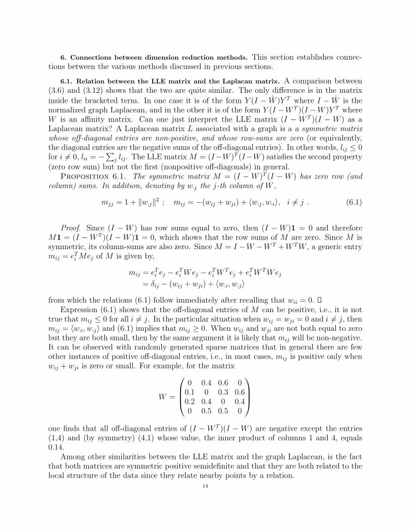


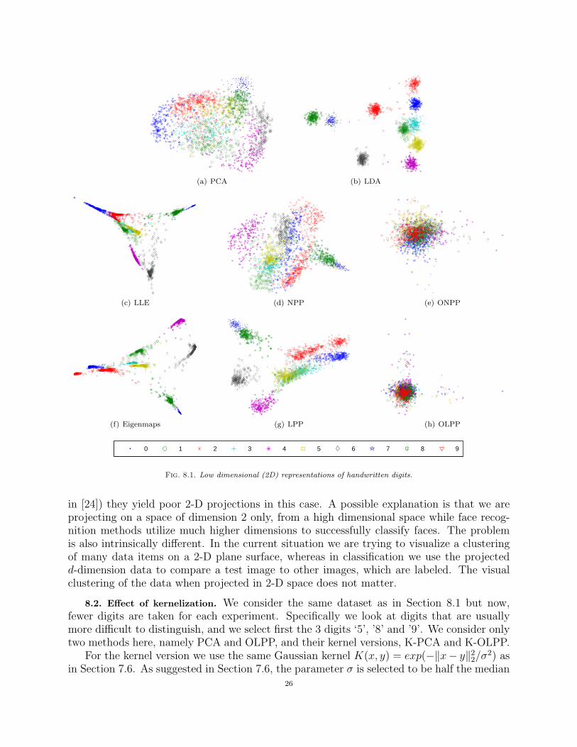
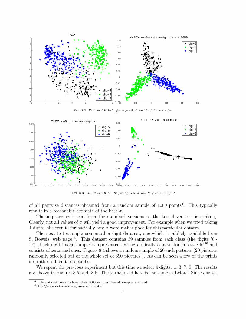


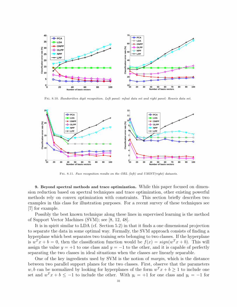


![TRACE OPTIMIZATION AND EIGENPROBLEMS IN DIMENSION ...saad/PDF/umsi-2009-31.pdf · Ham et al [21] note that several of the known standard methods (LLE [34], Isomap [46], Laplacean](https://static.documents.pub/doc/80x56/5d63cc6688c993635d8b4d60/trace-optimization-and-eigenproblems-in-dimension-saadpdfumsi-2009-31pdf.jpg)
