Tracer Testing Techniques to Support Design Tracer Testing Techniques to Support Design and Operation of In Situ Remediation Systems Craig E. Divine, PhD, PG ARCADIS Highlands Ranch (Denver), Colorado, USA Craig.Divine@arcadis‐us.com Remediation Technologies Symposium 2008 O b 2008 October 17, 2008 The Fairmont Banff Springs Hotel Banff, Alberta
Transcript
Tracer Testing Techniques to Support DesignTracer Testing Techniques to Support Design and Operation of In Situ Remediation Systems
Craig E. Divine, PhD, PGARCADIS
Highlands Ranch (Denver), Colorado, USA
Craig.Divine@arcadis‐us.coma g e@a cad s us co
Remediation Technologies Symposium 2008
O b 2008October 17, 2008
The Fairmont Banff Springs Hotel
Banff, Alberta
Applied TracersDefinition:Definition:
Unique constituent intentionally introduced to aquifer
Why Powerful:
Source term is controlled and well characterized
•~10 AD: Flavius Josephus: chaff tracer identifies source of Jordan R.
•Late 1800s: Quantitative tracer tests using fluorescent dyes, salt, and bacteria in karst aquifers
•1945‐1955: Advances in chemical measurement increased power and•1945 1955: Advances in chemical measurement increased power and made high‐frequency sampling economically feasible
•1965‐1970: 650 papers
1995‐2000: 6500+ papers
•Now routinely used in “non‐research” applications
– ARCADIS uses tracers to support design of all in situ systems– ARCADIS uses tracers to support design of all in situ systems
2
Aquifers are Heterogeneous and Anisotropic as a Rule!
Geology controls distribution and transport of injected fluids and solutesGeology controls distribution and transport of injected fluids and solutes•• The success of in situ remediation systems requires site specific understanding and tailored designThe success of in situ remediation systems requires site specific understanding and tailored design•• Tracer tests can effectively provide this critical informationTracer tests can effectively provide this critical information•• Tracer tests can effectively provide this critical informationTracer tests can effectively provide this critical information
“We need to stamp out homogeneous “We need to stamp out homogeneous isotropismisotropism from our thinking!”from our thinking!”
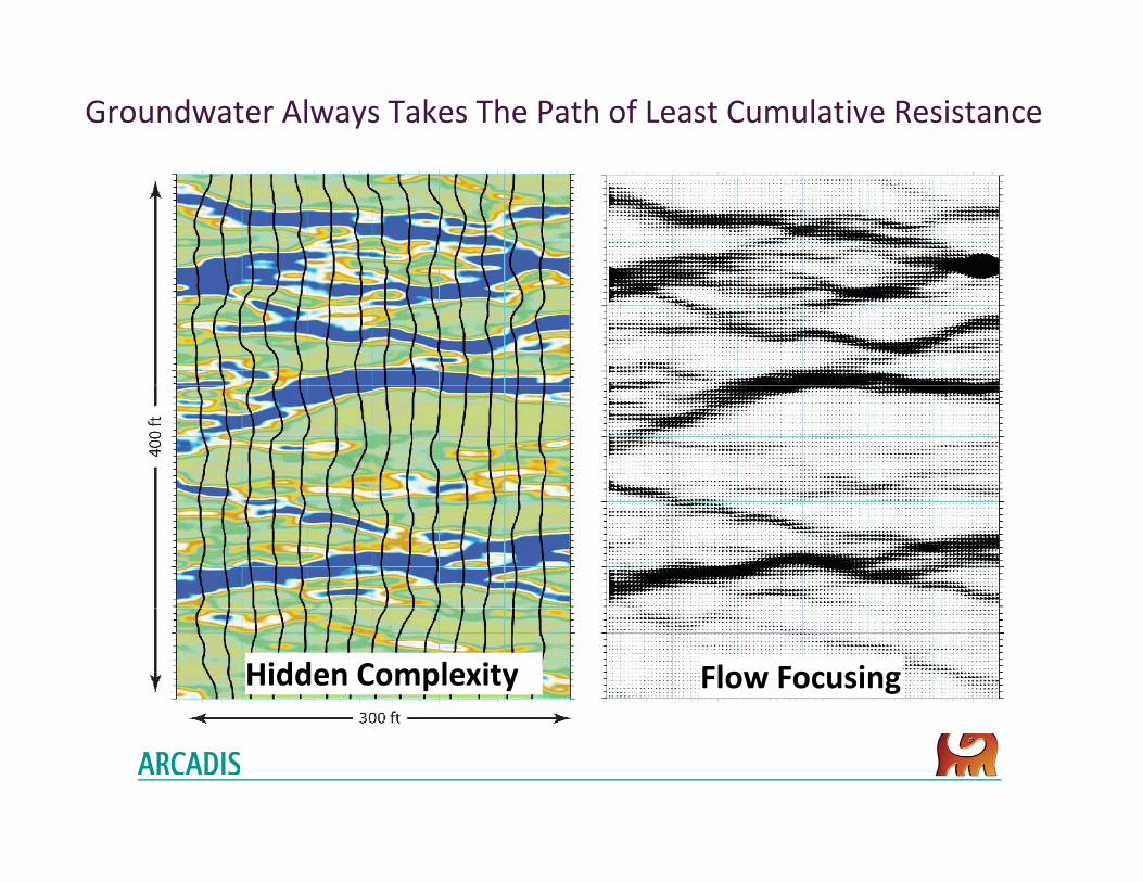
Groundwater Always Takes The Path of Least Cumulative Resistance
Flow FocusingHidden Complexity
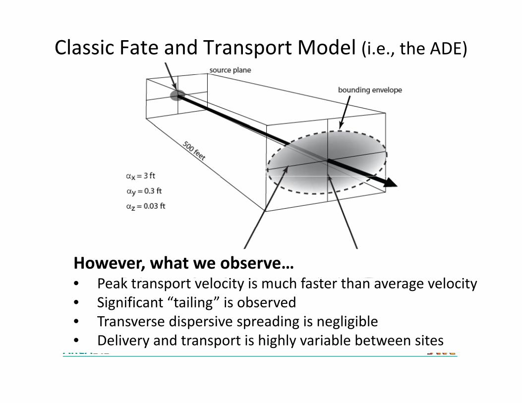
Classic Fate and Transport Model (i.e., the ADE)
However, what we observe…k l h f h l• Peak transport velocity is much faster than average velocity
• Significant “tailing” is observed• Transverse dispersive spreading is negligiblep p g g g• Delivery and transport is highly variable between sites
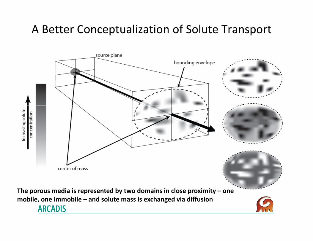
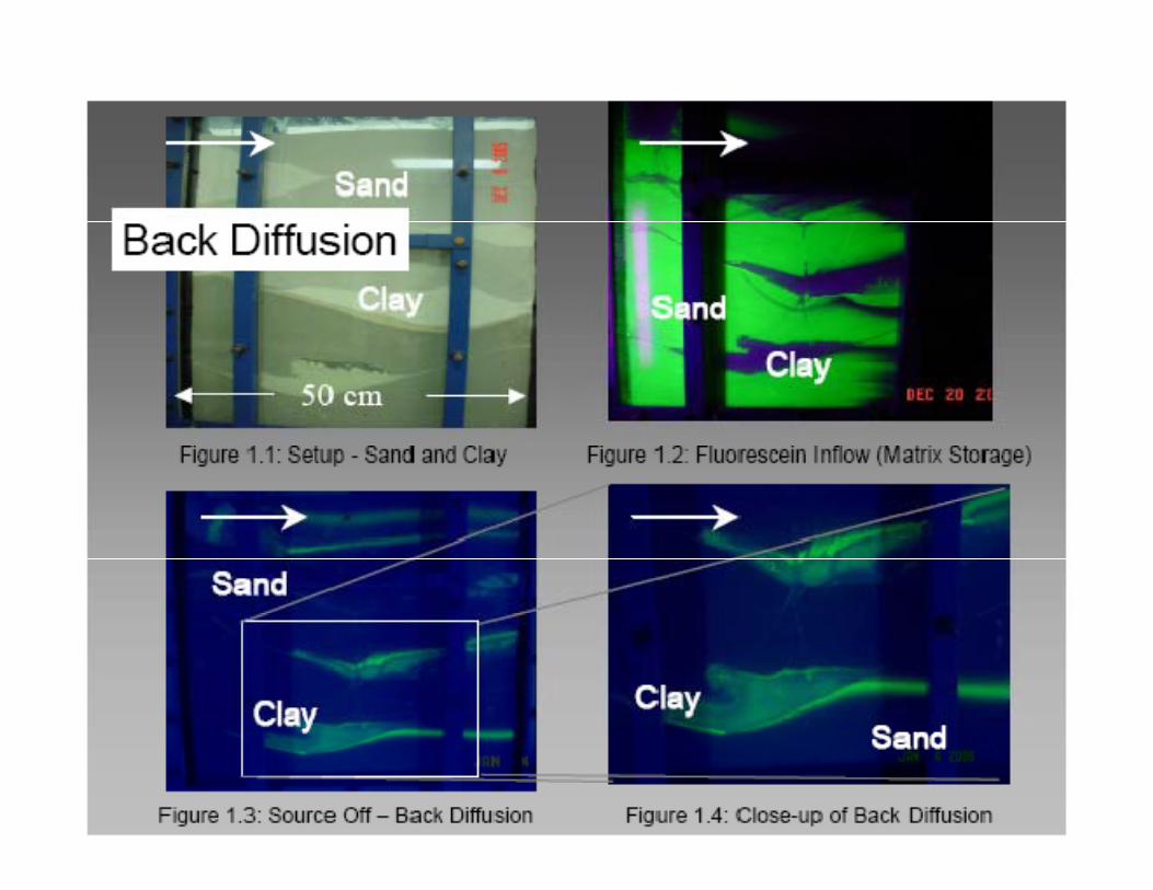
A Better Conceptualization of Solute Transport
The porous media is represented by two domains in close proximity – one mobile, one immobile – and solute mass is exchanged via diffusion
7
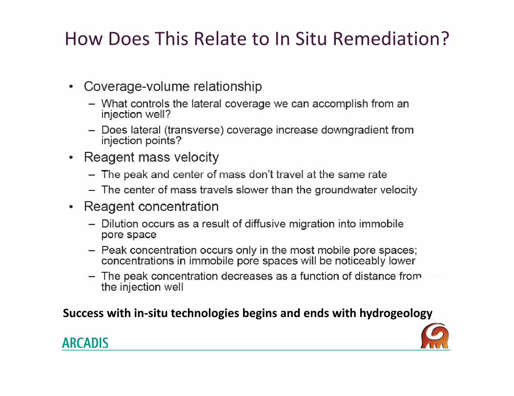
How Does This Relate to In Situ Remediation?
Success with in‐situ technologies begins and ends with hydrogeology
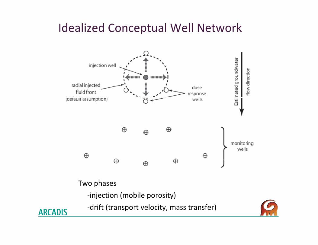
Idealized Conceptual Well Network
Two phases
‐injection (mobile porosity)
‐drift (transport velocity, mass transfer)
Injection Phase – Calculating Mobile Porosity
• Inject whatever volume is needed to reach a planned radius Monitor Tracer
rr
• Use a qualitative tracer to get real‐time arrival
1Average Velocity: 1 2 ft/dayMobile Porosity: 2‐4%Immobile Porosity: 25%M T f 0 05 d
0 40.50.60.7
ObservedMobileI bil
Mass Transfer: 0.05 per day
0.10.20.30.4 Immobile
010 20 30 40 50
Key Information Relevant to Design
• High hydraulic conductivityAquifer has high injectability– Aquifer has high injectability
• Low mobile porosity– Facilitates efficient amendment distribution
• Immobile porosity and mass‐transfer– Diffusion‐controlled tailing for conservative solutes will control period of performancep p
• May need to consider recirculation strategies for full‐scale implementation
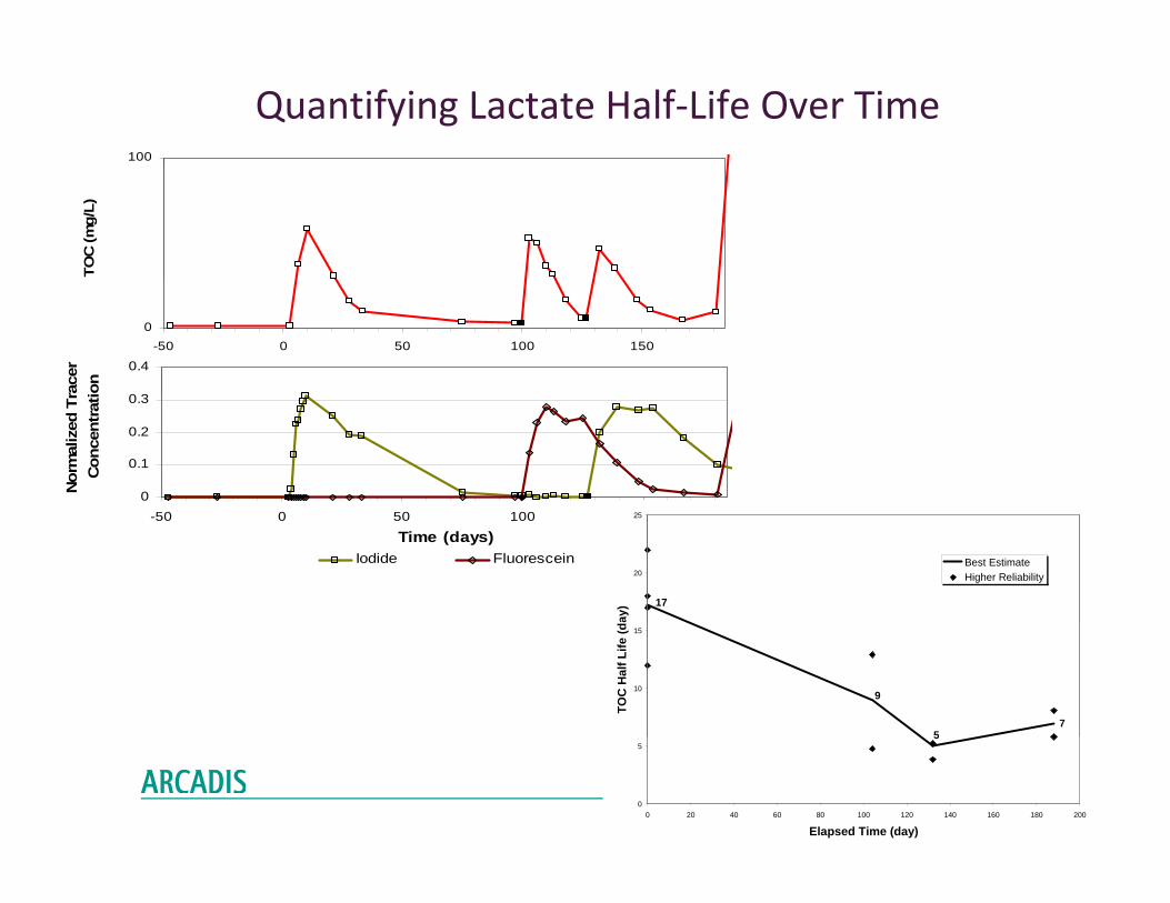
Quantifying Lactate Half‐Life Over Time100
TOC
(mg/
L)
0-50 0 50 100 150
Time (days)TOC
0 3
0.4
race
r io
n
0
0.1
0.2
0.3
Nor
mal
ized
Tr
Con
cent
rati
-50 0 50 100 150
Time (days)Iodide Fluorescein
17
20
25
ay)
Best EstimateHigher Reliability
75
910
15TO
C H
alf L
ife (d
5
0
5
0 20 40 60 80 100 120 140 160 180 200
Elapsed Time (day)
4D Mapping with Geophysics
Amendment 5 hrs after injection
15
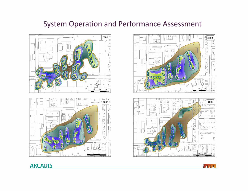
System Operation and Performance Assessment
IRZ Operation and Performance
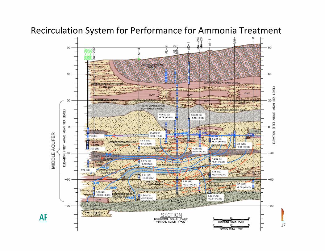
Recirculation System for Performance for Ammonia Treatment
17
Ethanol Recirculation System for Cr (VI) Treatment
184 0
230.0
138.0
184.0
Observed
C d
46.0
92.0 Computed
0.0
0.3 864.3 1,728.2 2,592.1 3,456.1 4,320.0
Time
Push‐Pull Test for Cr(VI) Sorption
300
400
(mg/
L)
0
100
200
0 500 1000 1500 2000 2500 3000 3500 4000
Bro
mid
e
0 500 1000 1500 2000 2500 3000 3500 4000
Extracted Volume(gal)
100
150
200
ium
(µg/
L)
0
50
0 500 1000 1500 2000 2500 3000 3500 4000
Chr
om
Extracted Volume (gal)
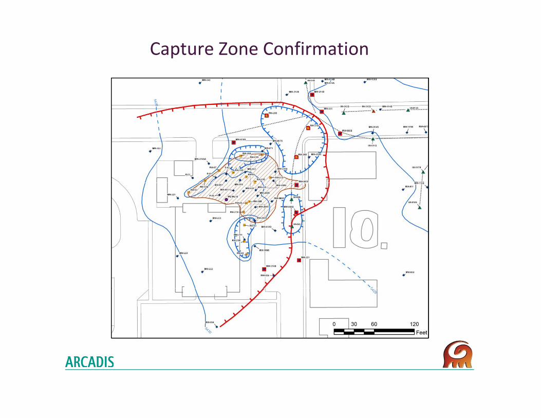
Capture Zone Confirmation
Future Directions•Improved in‐situ and “real‐time” monitoring capabilities
•Development of practical test design tools
•Measure LNAPL mobilityMeasure LNAPL mobility
Closing Thoughts“There’s no truth like tracer truth.” James Quinlan
Tracers are the best tools for understanding how injected fluids and contaminants beha e at the remediation (i e local ) scalecontaminants behave at the remediation (i.e., local ) scale
AcknowledgementsPayne, F.C, Quinnan, J.A., and Potter, S.T., 2008.
Remediation Hydraulics. CRC Press, Boca Raton, FL. 408 pp.