TRAVEL SPEED PREDICTION BASED ON LEARNING METHODS …

TRAVEL SPEED PREDICTION BASED ON

LEARNING METHODS FOR HOME

DELIVERY

Maha Gmira

Michel Gendreau

Andrea Lodi

Jean-Yves Potvin

November 2018

DS4DM-2018-012

POLYTECHNIQUE MONTRÉAL

DÉPARTEMENT DE MATHÉMATIQUES ET GÉNIE INDUSTRIEL

Pavillon André-Aisenstadt Succursale Centre-Ville C.P. 6079 Montréal - Québec H3C 3A7 - Canada Téléphone: 514-340-5121 # 3314

Travel Speed Prediction based on LearningMethods for Home Delivery

Maha Gmira †§¶, Michel Gendreau †¶Andrea Lodi †§¶, Jean-Yves Potvin ‡¶

†Departement de mathematiques et de genie industrielPolytechnique Montreal,

C.P. 6079, succ. Centre-Ville, Montreal, Quebec, Canada H3C 3A7.

‡Departement d’informatique et de recherche operationnelleUniversite de Montreal,

C.P. 6128, succ. Centre-Ville, Montreal, Quebec, Canada H3C 3J7.

§Chaire d’excellence en recherche du Canada sur la science des donneespour la prise de decision en temps reel

Polytechnique Montreal,C.P. 6079, succ. Centre-Ville, Montreal, Quebec, Canada H3C 3A7.

¶Centre interuniversitaire de recherchesur les reseaux d’entreprise, la logistique et le transport,

Universite de Montreal,C.P. 6128, succ. Centre-Ville, Montreal, Quebec, Canada H3C 3J7.

Abstract. The travel time required to get from one location to another in a network isan important performance measure in intelligent transportation and advanced travelerinformation systems. Accordingly, accurate travel time predictions are of foremostimportance. In an urban environment, vehicle speed and consequently travel time canbe highly variable due to congestion caused, for example, by accidents or bad weatherconditions. At another level, one also observes daily patterns (e.g., rush hours),

1

CERC DATA SCIENCE FOR REAL-TIME DECISION-MAKING DS4DM-2018-012

weekly patterns (e.g., weekdays versus weekend), and seasonal patterns. Capturingtime-varying features when modeling travel speeds provide an immediate benefit tocommercial transportation companies that distribute goods, since it allows them tobetter optimize their routes and reduce their environmental footprint.

This paper presents a travel speed prediction methodology based on data collectedfrom mobile location devices installed inside commercial delivery vehicles. An analysisis conducted using unsupervised learning to cluster data, dimensionality reductiontechniques and imputation methods to fill missing values and a Long Short-TermMemory neural network to forecast travel speeds.

1 IntroductionTraffic congestion can be classified as recurrent (due to well-known patterns) andnon-recurrent (due to accidents, construction, emergencies, special events and badweather, among others). Accordingly, there is a need for models that can derive futurevalues from observed trends, in order to provide accurate predictions under recurrentand non-recurrent congestion. With the increasing amount of available data collectedfrom probe vehicles, smartphone’s applications and other location technologies, thechallenge is no longer related to the quantity of data but rather to the modeling andextraction of useful information from such data. This information can be of greatvalue for transportation companies operating in urban areas.

Given the variability of travel speeds due to usual and unusual traffic situations,the objective of this research is to make better travel speed predictions, which shouldultimately help to generate better vehicle delivery routes. This will be done witha neural network model that uses information extracted from data collected frommobile location devices. The data for this study come from a software developmentcompany located in Montreal that produces vehicle routing algorithms to plan thehome delivery of large items (appliances, furniture) to customers. This partner hasdelivery routes with more than 2,500,000 delivery points, serviced by nearly 200,000routes. Data are collected using Automatic Vehicle Location (AVL) systems whereGPS receivers are usually interfaced with Global System for Mobile Communications(GSM) modems. The system records point locations as latitude-longitude pairs, in-stantaneous speed, date and time. Our challenge here was to develop techniques forthe management of big data that would allow prediction algorithms to perform well.

In the following, a review of the scientific literature related to our work is firstpresented in Section 2. Then, our methodology for travel speed prediction is reported.The creation of a database of speed patterns from GPS traces is described in Section3. Then, techniques to reduce the size of the database and cluster arcs into similarityclasses are explained in Section 4. This is followed by the neural network model used

2


to predict travel speeds in Section 5. Computational results are finally reported inSection 6.

2 Literature reviewMost urban traffic control systems rely on short-term traffic prediction and a hugeliterature has been published on this topic in the last decades due, in particular, tothe advent of Intelligent Transportation Systems (ITS). Given that these systems arehighly dependent on accurate traffic information, they must collect a large amountof data (locations, speeds and individual itineraries).

Travel speed prediction at a given time typically relies on historical travel speedvalues and a set of exogenous variables. Methods to predict traffic information areclassified in [49] as 1) naive (i.e., without any model assumption), 2) parametric, 3)non-parametric and 4) a combination of the last two, called hybrid methods. Thefirst three methods are described in the following.

2.1 Naive methodsNaive methods are by far the easiest to implement and to use because they do notrequire an underlying model. However, one main drawback is their lack of accuracy. In[49], naive methods are divided into instantaneous methods (based on data availableat the instant the prediction is performed), historical methods (based on historicaldata) and mixed methods, where the latter combine characteristics of historical andinstantaneous methods. As a baseline for comparison with other parametric methods,the work reported in [44] uses a simple hybrid method where the travel speed forecastis a function of the current traffic flow rate, as well as its historical average at a giventime of the day and day of the week. In [57], the authors compare two methods fortravel time prediction, one based on data available at the instant the prediction isperformed and one based on historical data. Using the Relative Mean Error (RME)and the Root Mean Squared Error (RMSE), these two approaches showed similarperformance, but were clearly outperformed by a more sophisticated approach calledSupport Vector Regression (see Section 2.3).

2.2 Parametric methodsParametric methods use data to estimate the parameters of a model, whose structureis predetermined. The most basic model is linear regression, where the traffic variableVt to be predicted at a given time t is a linear function of independent variables:

Vt = β0 + β1X1 + β2X2 + ...+ βnXn . (1)

3


Different techniques are available to estimate the parameters βi, i = 1, ... n. Amongparametric methods, we consider the Autoregressive Moving Average model (ARMA)and its Integrated variant (ARIMA), different smoothing techniques and the Kalmanfilter. They are presented below.

(a) Kalman FilterThe Kalman filter is a very popular short-term traffic flow prediction method. Itallows the state variables to be updated continuously, which is very importantin time-dependent contexts. Some works related to traffic state estimationare based on the original Kalman filter [28], as well as its extension for non-linear systems called the Extended Kalman Filter (EKF) [27]. The latter isparticularly relevant since the travel times depend on traffic conditions thatare highly non-linear and dynamic, changing over time and space. In [55], afreeway state estimator is obtained by solving a macroscopic traffic flow modelwith EKF. A new EKF based on online-learning is used in [50] to provide traveltime information on freeways. Also, a dynamic traffic assignment model, whichis a non-linear state-space model, is solved by applying three different extensionsof the Kalman filter [1].In [26], the authors use traffic data on California highways to predict traveltimes on arcs and estimate the arrival time at a destination. First, travel timeson arcs are predicted by feeding the Kalman filter with historical data. Then,this prediction is corrected and updated with real time information using theKalman filter’s corrector-predictor form.

(b) ARMATo predict short-term traffic characteristics such as speed, flow or travel time,time series models based on ARMA(p,q) (which is a combination of p autore-gressive terms AR and q moving average terms MA) have been widely used. Ifwe consider travel time prediction, the general formulation of ARMA(p,q) is:

T (t)−p∑

i=1αiT (t− i) = Z(t) +

q∑j=1

βjZ(t− j) , (2)

where the travel time T (t), given departure time t, is a linear function of thetravel times at previous instants, Z(t− 1), .... , Z(t− q) are noise variables and(αi, βj) are parameters.ARIMA models generalize ARMA models for non-stationary time series. Theyrely on stochastic system theory since the processes are non-deterministic. In[22], the authors use the Box-Jenkins approach [4] to develop a forecasting model

4


based on ARIMA from data collected in urban streets (i.e., 1-minute traffic-volume on each street during peak periods). After comparing several ARIMAmodels, the one of order (0,1,1) yielded the best results in terms of traffic volumeforecasts, where the values of 0, 1 and 1 refer to the order of the autoregressivemodel (number of time lags), number of differentiation steps (number of timesthe values in the past are subtracted) and moving-average terms, respectively.The authors in [44] compare a seasonal ARIMA model, called SARIMA, witha non-parametric regression model where the forecast generation method andneighbor selection criteria are heuristically improved. The tests showed thatSARIMA performed better than the improved non-parametric regression.In [56], the authors model traffic flow with SARIMA (1,0,1) and SARIMA(0,1,1)models. Another SARIMA model is reported in [20] to forecast traffic conditionsover a short-term horizon, based on 15-minute traffic flow data. In this case,SARIMA outperformed the K-nearest neighbor method.

2.3 Non-parametric methodsNon-parametric methods include non-parametric regression and different types ofneural networks. Non-parametric methods are also known as data-driven methods,because they need data to determine not only the parameters but also the modelstructure. Thus, the number and types of parameters are unknown a priori. Themain advantage of these methods is that they do not require expertise in traffic the-ory, although they need a lot of data.

The most popular non-parametric methods for traffic prediction are the supportvector machine, neural networks and non-parametric regression.

(a) Support Vector MachineThe Support Vector Machine (SVM) was first introduced in [51, 52] and usedin many classification and regression studies. SVM is popular because it guar-antees global minima, it deals quite well with corrupted data and works forcomplex non-linear systems. Support Vector Regression (SVR) is the applica-tion of SVM to time-series forecasting.In [57], the authors analyze the application of SVR for travel time prediction.They used traffic data, obtained from an Intelligent Transportation System, overa five weeks period. The first four weeks correspond to the training set and thelast week corresponds to the testing set. Using a Gaussian kernel function anda standard SVR implementation, their method improved the RME and RMSEwhen compared to instantaneous and historical travel time prediction methods.

5


Due to its promising results, SVR has been used to predict traffic parameterssuch as traffic flow or travel time. However, the classical SVR, like the one usedin [57], cannot be applied in real time because it requires a complete modeltraining each time a new record (data) is added. There are also some variantsof SVM for traffic prediction. In [54], the authors report a hybrid model calledthe chaos-wavelet analysis SVM that overcomes the need to choose a suitablekernel function. In the context of traffic flow prediction for a large-scale roadnetwork [58], SVM parameters are optimized by a parallel genetic algorithm,thus yielding a Genetic Algorithm-Support Vector Machine (referred to as GA-SVM).

(b) Neural networksWhen considering data-driven methods, neural networks are among the bestfor traffic forecasting because of their ability to learn non-linear relationshipsamong different features without any prior assumption.The most widely used neural networks are called Multi-Layer Perceptrons (MLPs).They are typically made of an input layer, one hidden layer and an output layer,where each layer contains one or more units (neurons). The units in the inputlayer are connected to those in the hidden layer, while the units in the hiddenlayer are connected to those in the output layer. The weights on these con-nections are adjusted during the learning process using (input, target output)example pairs, so as to produce an appropriate mapping between the inputs andthe target outputs. In [8], a MLP is used to predict traffic flow from input data(speed, flow, occupancy) collected by detection devices on a highway aroundthe city of London. In that application, the MLP and a radial basis functionnetwork performed better than all ARIMA models considered. In [53], the au-thors exploit a genetic algorithm to fine tune the parameters and the number ofhidden units in a MLP. Their model showed better generalization abilities whentested with new inputs. More recently, the authors in [21] report the perfor-mance of a MLP with 15 hidden units, trained with the Levenberg-Marquardtbackpropagation algorithm. Based on different error performance indicators,the MLP showed good accuracy when predicting road speeds. In [34], a MLPis used to predict the time needed to cross the Ambassador bridge, one of thebusiest bridges at the Canada-US border. A database of GPS records for a fullyear was used to train and test the neural network.As indicated in [32], Recurrent Neural Networks (RNNs) are better suited fortraffic forecasting tasks due to their ability to account for sequential time-dependent data. Typically, the signal sent by the hidden layer to the outputlayer at some time t is also sent back to the hidden layer. This signal is pro-

6


cessed with the input signal at time t + 1 to determine the internal state ofthe hidden layer. This internal state acts as a memory and remembers usefultime-dependent relationships among data.A specific class of RNNs, called Long Short-Term memories (LSTM), is nowwidely used in the literature due to its proven ability to learn long-term rela-tionships in the data. In [32], LSTM is compared to various RNNs and otherstatistical methods, namely: Elman neural network, non-linear autoregressivewith exogenous inputs (NARX) neural network, Time-Delay Neural Network(TDNN), SVM, ARIMA and Kalman filter. The LSTM achieved the best per-formances in terms of accuracy and stability. The work in [48] proposes a LSTMmodel for short-term traffic flow prediction and compared it with Random Walk(RW), SVM, MLP and Stacked Autoencoder (SAE). The results showed thesuperiority of LSTM in terms of prediction accuracy, ability to memorize long-term historical data and generalization capabilities. In [15], LSTM and a neuralnetwork model made of Gated Recurrent Units (GRUs) [9] are applied to trafficdata in California. The study showed that GRUs behave slightly better thanLSTM, while both outperformed an ARIMA model in terms of Mean SquaredError (MSE) and Mean Absolute Error (MAE).

(c) Non-parametric regressionAnother class of non-parametric methods is called Non-Parametric Regression(NPR). It is suitable for short-term traffic prediction since it can deal with theuncertainty in traffic flows. The objective of NPR is to estimate a regressionfunction without relying on an explicit form, unlike the traditional parametricregression models (where the model parameters are estimated). The forecastingability of NPR relies on a database of past observations. It applies a searchprocedure to find observations in this database that are similar to the currentconditions. Then, it transfers these observations to the forecast function toestimate the future state of the system.The k-Nearest Neighbor (k-NN) is a widespread class of non-parametric regres-sion methods made of two components:

(i) Search procedure: the nearest neighbors (historical data most similar to thecurrent input) are the inputs to the forecast function aimed at generatingan estimate. The nearest neighbors are found using a similarity measure,which is usually based on the Minkowski distance metric:

Lr =(

n∑i=1|pi − qi|r

)1/r

, (3)

7


where n is the dimension of the state vector, pi is the ith element of thehistorical record currently considered, qi is the ith element of the currentconditions, and r is a parameter with values between 1 and 2. The mostcommon implementation uses a sequential search procedure. However,as the number of historical observations increases, the sequential searchbecomes very time consuming.

(ii) Forecast function: the most general approach to generate a prediction isto compute an average of the dependent variable values over the nearestneighbors. However, this approach ignores the information provided by thedistance metric (i.e., past observations closer to the current input shouldhave more impact on the forecast).

The authors in [10] were among the first to use NPR to estimate short-termtraffic flows. Their work highlighted the importance of a large and represen-tative dataset. NPR was then applied to estimate traffic volumes from twosites located in Northern Virginia Capital Beltway, based on five months ofobservations [42]. The results showed that the proposed method can gener-ate more accurate predictions than the other tested approaches (including aneural network model). The work in [43] compares historical averages, timeseries, back-propagation neural networks and non-parametric regression modelsusing a performance index that includes absolute error, error distribution, easeof model implementation and model portability. Overall, NPR proved to bebetter than the other models and was also easier to implement.

The interested reader is referred to [13] for a more exhaustive review on traf-fic forecasting. The following sections will now describe the various steps that weperformed to produce travel speed predictions from our huge database.

3 Deriving speed patterns from GPS tracesOur industrial partner provided us with one year and a half of GPS data transmit-ted by mobile devices installed in delivery vehicles (extending over the years 2013,2014 and 2015). These GPS points were first mapped to the underlying MontrealMetropolitan Community (MMC) network to generate daily speed patterns for eachindividual arc, where a daily speed pattern for a given arc is made of 96 averagespeeds taken over time intervals of 15 minutes.

In the following, the main issues related to the derivation of speed patterns fromGPS traces are briefly discussed.

8


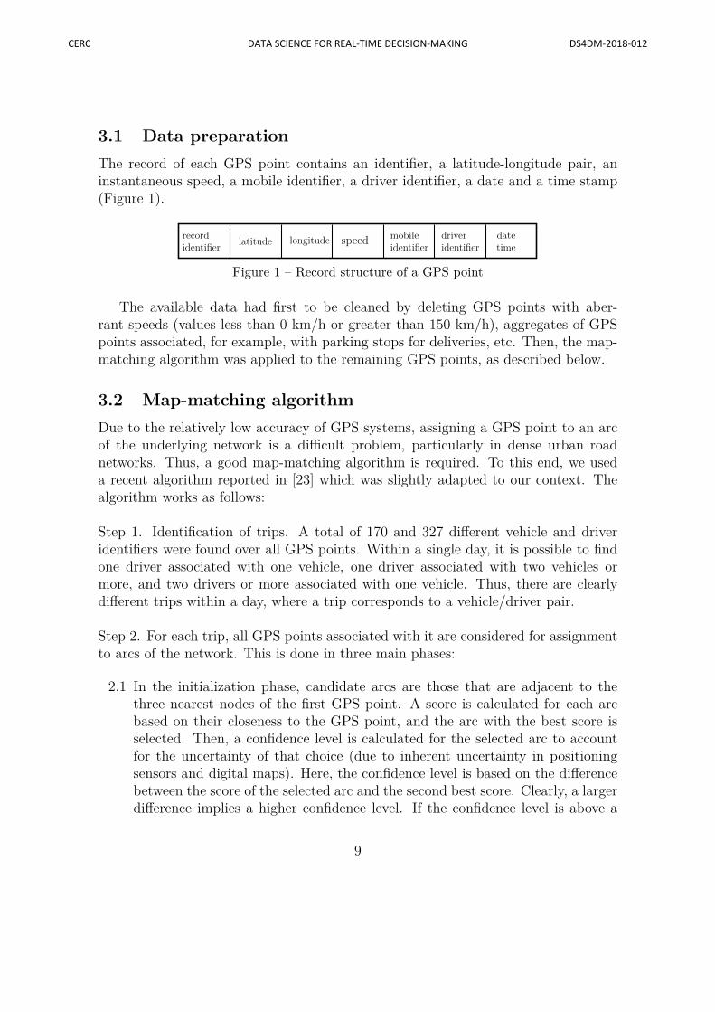
3.1 Data preparationThe record of each GPS point contains an identifier, a latitude-longitude pair, aninstantaneous speed, a mobile identifier, a driver identifier, a date and a time stamp(Figure 1).

recordidentifier latitude longitude speed mobile

identifierdriveridentifier

datetime

Figure 1 – Record structure of a GPS point

The available data had first to be cleaned by deleting GPS points with aber-rant speeds (values less than 0 km/h or greater than 150 km/h), aggregates of GPSpoints associated, for example, with parking stops for deliveries, etc. Then, the map-matching algorithm was applied to the remaining GPS points, as described below.

3.2 Map-matching algorithmDue to the relatively low accuracy of GPS systems, assigning a GPS point to an arcof the underlying network is a difficult problem, particularly in dense urban roadnetworks. Thus, a good map-matching algorithm is required. To this end, we useda recent algorithm reported in [23] which was slightly adapted to our context. Thealgorithm works as follows:

Step 1. Identification of trips. A total of 170 and 327 different vehicle and driveridentifiers were found over all GPS points. Within a single day, it is possible to findone driver associated with one vehicle, one driver associated with two vehicles ormore, and two drivers or more associated with one vehicle. Thus, there are clearlydifferent trips within a day, where a trip corresponds to a vehicle/driver pair.

Step 2. For each trip, all GPS points associated with it are considered for assignmentto arcs of the network. This is done in three main phases:

2.1 In the initialization phase, candidate arcs are those that are adjacent to thethree nearest nodes of the first GPS point. A score is calculated for each arcbased on their closeness to the GPS point, and the arc with the best score isselected. Then, a confidence level is calculated for the selected arc to accountfor the uncertainty of that choice (due to inherent uncertainty in positioningsensors and digital maps). Here, the confidence level is based on the differencebetween the score of the selected arc and the second best score. Clearly, a largerdifference implies a higher confidence level. If the confidence level is above a

9


given threshold, the GPS point is assigned to the selected arc, otherwise it isskipped and the next GPS point is considered. Once a GPS point is assignedto the first arc, the same-arc phase starts.

2.2 In the same-arc phase, the next GPS point is assigned to the same arc thanthe previous one, unless some conditions are not satisfied anymore (e.g., whencrossing an intersection). In the latter case, the algorithm switches to the next-arc phase.

2.3 In the next-arc phase, candidate arcs are those connected to the previouslyselected arc plus those that are adjacent to the three nearest nodes of the currentGPS point. A score is calculated for each arc based on its closeness to the GPSpoint and the difference in direction between the arc and the line connectingthe previous GPS point to the current one. Again, the arc with the best scoreis selected, its confidence level is calculated, and topological constraints arechecked (e.g., arc not connected to the previous one, turn restrictions, etc.).Depending on the confidence level and satisfaction of the topological constraints,the current GPS point can either be skipped or assigned to the new arc. In thelatter case, the algorithm returns to the same-arc phase. It should be noted thatconsidering arcs that are close to the current GPS point, but not necessarilyconnected to the previous arc, allows the algorithm to account for discontinuitiesin GPS traces due to obstacles (e.g., tunnels, bridges).

The interested reader is referred to [23] for details about this algorithm.

When the assignment of GSP points to arcs is completed for each day, averagetravel speeds can be calculated over time slots of 15 minutes. Thus, a new databaseis obtained where each record has the structure shown in Figure 2. The next sectionwill now explain how this database was exploited to fit our purposes.

arcidentifier date day season 00:00AM ............. 11:45PM

96 avg. speed valuestemporal characteristicsFigure 2 – Database structure after geomatic analysis

10


4 Size reduction and clusteringDue to the size of our database, size reduction techniques were applied. After elim-inating speed patterns and hours with too many missing data, a “prediction-after-classification” approach was used to cluster arcs with similar speed patterns intoclasses before predicting travel speed values. This is explained in the following.

4.1 Database reductionWith 233,914 arcs and 515 days in the database, we have a total of 233,914 × 515= 120,506,910 speed patterns. Originally, the database was constructed with timeintervals of 15 minutes. That is, a speed pattern for a given arc on a given day ismade of 96 average speed values taken over time intervals of 15 minutes, thus coveringan horizon of 24 hours. Furthermore, the speed limit was stored when no observationwas recorded within a 15-minute time interval.

An elimination procedure was first applied to get rid of speed patterns or timeintervals with too few data, as described below.

(a) Speed patterns. To keep only average speed values based on real observations,the speed limit values were removed from the database. Given that a significantproportion of the resulting speed patterns now contained missing data, a speedpattern was automatically discarded when the proportion of real average speedvalues over the 96 time intervals was less than 5% (note that this threshold isoften suggested in the literature). In other words, a speed pattern with only 4average speeds or less was eliminated. Through this process, we ended up witha total of 6,667,459 speed patterns. It should be noted that only 3,485 arcs stillhad at least one representative speed pattern in this database. The fact thatthe original GPS traces have been collected from delivery routes in particularsectors of an urban area explains this large reduction in the number of arcs andspeed patterns. Finally, the 96 time intervals of 15 minutes of each remainingspeed pattern were aggregated into 24 one-hour time intervals, to allow thecalculation of average speed values based on more observations in each timeinterval, see Figures 3 and 4.

(b) One-hour time intervals. After reducing the number of speed patterns in thedatabase, as well as the number of average speed values stored in a pattern, wethen examined more closely the one-hour time intervals.

11


0 50000 100000 150000 200000

00:00AM00:15AM00:30AM00:45AM01:00AM01:15AM01:30AM01:45AM02:00AM02:15AM02:30AM02:45AM03:00AM03:15AM03:30AM03:45AM04:00AM04:15AM04:30AM04:45AM05:00AM05:15AM05:30AM05:45AM06:00AM06:15AM06:30AM06:45AM07:00AM07:15AM07:30AM07:45AM08:00AM08:15AM08:30AM08:45AM09:00AM09:15AM09:30AM09:45AM10:00AM10:15AM10:30AM10:45AM11:00AM11:15AM11:30AM11:45AM00:00PM00:15PM00:30PM00:45PM01:00PM01:15PM01:30PM01:45PM02:00PM02:15PM02:30PM02:45PM03:00PM03:15PM03:30PM03:45PM04:00PM04:15PM04:30PM04:45PM05:00PM05:15PM05:30PM05:45PM06:00PM06:15PM06:30PM06:45PM07:00PM07:15PM07:30PM07:45PM08:00PM08:15PM08:30PM08:45PM09:00PM09:15PM09:30PM09:45PM10:00PM10:15PM10:30PM10:45PM11:00PM11:15PM11:30PM11:45PM

Number of observations

Figure 3 – Number of observations per time interval of 15 minutes

12


0 250000 500000 750000

00:00AM

01:00AM

02:00AM

03:00AM

04:00AM

05:00AM

06:00AM

07:00AM

08:00AM

09:00AM

10:00AM

11:00AM

00:00PM

01:00PM

02:00PM

03:00PM

04:00PM

05:00PM

06:00PM

07:00PM

08:00PM

09:00PM

10:00PM

11:00PM

Number of observations

Figure 4 – Number of observations per time interval of 1 hour

13


Clearly, there are intervals with no or very few observations over the entiredatabase, like night hours (although some observations can be found in thedatabase because the vehicles are sometimes moved during the night from onelocation to another). Accordingly, we discarded hours where the proportion ofreal average speed values over the 6,667,459 speed patterns in the database wasunder 5%. After this elimination process, the number of one-hour time intervalswas reduced from 24 to 13. More precisely, only one-hour time intervals startingfrom 7:00 AM to 7:00 PM were kept in every speed pattern.

4.2 ClusteringWhen this step is reached, we have a database of 6,667,459 speed patterns, whereeach pattern is associated with a given arc and a given date. A speed pattern canbe seen as a vector of 13 average speed values, one for each one-hour time intervalstarting from 7:00 AM to 7:00 PM. This number of speed patterns is still too large tobe processed by a learning-based prediction algorithm, so we had to group arcs withsimilar patterns into a number of classes. For this purpose, an average speed patternwas calculated for each arc over all its corresponding speed patterns in the database.Since 3,485 arcs are represented in the database, this led to N = 3,485 average speedpatterns.

In the following, the clustering methods used to identify classes of arcs are de-scribed.

4.2.1 K-means

To cluster arcs based on their average speed pattern with the K-means algorithm,the distance between two patterns was calculated using the Euclidean metric (see, forexample, [33]). At the end, K cluster centroids (classes) were obtained and the speedpattern of each arc was assigned to the closest centroid. Since the number of classesmust be fixed in advance, the latter was purposely set to a large value, i.e., K =200. Then, the output of the K-means algorithm was fed to a hierarchical clusteringmethod to further reduce the number of classes (see Section 4.2.2).

The problem solved by the K-means algorithm is summarized below, where Ck

stands for class k. The objective is to minimize the sum of the squares of the Euclideandistance between speed pattern xi of arc i and its closest centroid µk, over all arcs.In this objective, the variables are the µk’s.

MinK∑

k=1

∑xi∈Ck

‖xi − µk‖2 , (4)

14


where:Ck = {xi : ‖xi − µk‖ = min

l=1,...,K‖xi − µl‖} , (5)

µk = 1|Ck|

∑xi∈Ck

xi . (6)

An iterative method known as Lloyd’s algorithm was used to converge to a localminimum, given that solving the problem exactly is NP-hard. In this algorithm,starting from K randomly located centroids, the following two steps are performedrepeatedly until convergence is observed: 1) Cluster assignment: construct the set ofclasses by assigning each arc to the cluster centroid that is closest to the arc’s speedpattern and 2) Update centroids: update the centroid of each cluster by averagingover all speed patterns assigned to it.

4.2.2 Affinity propagation algorithm

The Affinity Propagation (AP) algorithm is a clustering procedure proposed in [14].As opposed to K-means, every data point is considered as a potential centroid.Through the propagation of so-called affinity values among pairs of data points, whichreflect the current affinity (or consent) of one data point to consider the other datapoint as its centroid, some data points accumulate evidence to be centroids. Thereader will find in [14] the exact mathematical formulas that are used to guide thetransmission of affinity values and the accumulation of evidence in data points. Atthe end, evidence is located only on a certain number of data points that are chosenas cluster centroids. Then, the set of classes is constructed by assigning each datapoint to its closest centroid. It should be noted that the centroids necessarily cor-respond to data points and that the number of classes does not need to be fixed inadvance. That is, the number of classes will automatically emerge as the algorithmunfolds. The authors in [14] also show that AP approximately minimizes the sumof the squares of the Euclidean distance between each data point and its assignedcentroid.

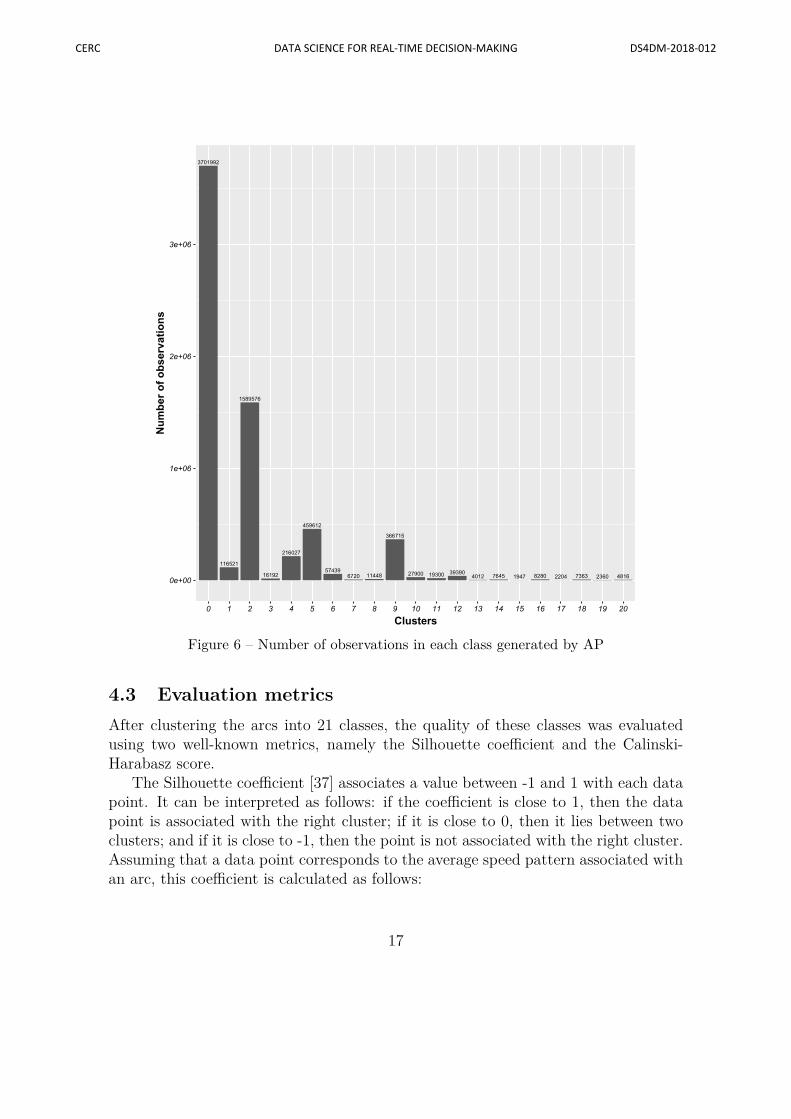
AP was applied using the centroids of the 200 classes produced by K -means asdata points. At the end, these 200 classes were aggregated into 21 different classes,labeled from 0 to 20. Figures 5 and 6 show the number of arcs and observations,respectively, in each class.

It should be noted that it was not possible to apply AP directly to the N = 3,485average speed patterns, which proved to be too large. This is the reason for the two-phase process, where K-means is applied first to reduce the problem size, followed byAP in the second phase. We also tested another clustering algorithm, known as theMean Shift Algorithm [16], but since it proved to be worse than AP, we will omit itsdescription.

15


0

10

20

30

0 1 2 3 4 5 6 7 8 9 10 11 12 13 14 15 16 17 18 19 20

Clusters

Num

ber o

f arc

s

Figure 5 – Number of arcs in each class generated by AP

16


3701992

116521

1589576

16192

216027

459612

574396720 11448

366715

27900 19300 393904012 7645 1947 8280 2204 7363 2360 48160e+00

1e+06

2e+06

3e+06

0 1 2 3 4 5 6 7 8 9 10 11 12 13 14 15 16 17 18 19 20

Clusters

Num

ber o

f obs

erva

tions

Figure 6 – Number of observations in each class generated by AP

4.3 Evaluation metricsAfter clustering the arcs into 21 classes, the quality of these classes was evaluatedusing two well-known metrics, namely the Silhouette coefficient and the Calinski-Harabasz score.

The Silhouette coefficient [37] associates a value between -1 and 1 with each datapoint. It can be interpreted as follows: if the coefficient is close to 1, then the datapoint is associated with the right cluster; if it is close to 0, then it lies between twoclusters; and if it is close to -1, then the point is not associated with the right cluster.Assuming that a data point corresponds to the average speed pattern associated withan arc, this coefficient is calculated as follows:

17


• for every arc i, calculate the average distance between its speed pattern and thespeed pattern of all other arcs in the same class; we call this value ai.

• for every arc i, calculate the average distance between its speed pattern and thespeed patterns of all arcs in the closest cluster; we call this value bi.

• the silhouette coefficient si of arc i is then:

si = bi − ai

max(ai, bi). (7)

At the end, the final value is the average of those si coefficients over all arcs.

The Calinski-Harabasz score [7] is another measure that provides a ratio betweenintra-class and inter-classes dispersion values. The clusters are better defined whenthe score is higher. The score is computed as follows:

CH(K) = Tr(B(K))Tr(W (K)) ∗

N −KK − 1 , (8)

where

W (K) =K∑

k=1

∑x∈C(k)

(x− c(k))(x− c(k))ᵀ , (9)

B(K) =K∑

k=1n(k)(c(k) − c)(c(k) − c)ᵀ . (10)

In these equations, a vector should be viewed as a column. Also, K is the numberof clusters or classes, N is the number of speed patterns (arcs), W (K) is the intra-cluster dispersion matrix, B(K) is the inter-cluster dispersion matrix, Tr(M) is thetrace of matrix M , C(k) is the set, of cardinality n(k), of speed patterns (arcs) in classk, c(k) is the centroid of speed patterns in class k and c is the centroid of all speedpatterns.

Note that each entry (i, j) in matrices W (K) and B(K) corresponds to:

W(K)ij =

K∑k=1

∑x∈C(k)

(xi − c(k)i )(xj − c(k)

j ) , (11)

B(K)ij =

K∑k=1

n(k)(c(k)i − ci)(c(k)

j − cj) . (12)

18


When the Silhouette coefficient was evaluated on the 21 classes produced by AP,a value of 0.85 was obtained. This is quite good, given that 1 is the best possiblevalue (note that the coefficient for the clusters produced by the Mean Shift algorithmwas equal to 0.67). Concerning the Calinski-Harabasz score, a value of 10.52 wasobtained, which is to be compared with 3.39 for the Mean Shift algorithm.

By focusing on the four classes with the largest number of observations, namelyclasses 0, 2, 5 and 9, we observed that the average speeds of classes 0, 2 and 5 arevery different, ranging from approximately 25 to 45 km/hour. The average speed ofclass 9 is similar to the one of class 2, but it does not evolve in the same way overthe day. When we looked at more detailed data, we observed that the arcs of class9 are not affected by the congestion observed during weekdays. That is, as opposedto classes 0, 2 and 5, there is no significant difference between the weekday averagespeeds and the weekend average speeds. Thus, the clustering algorithm was successfulin identifying classes of arcs with different characteristics.

5 Speed predictionThis section describes the supervised neural network model for predicting travelspeeds based on the classes generated by the AP clustering algorithm. Since a datamissing issue emerges in this context, we will first explain how this problem is handled.Then, the neural network model will be described.

5.1 Missing dataGiven that input vectors for the neural network model are obtained by averagingspeeds over all arcs in a class produced by our clustering methodology, there is nomissing data in the input (see Section 6.1). However, each target output vectorcorresponds to one of the 6,667,459 speed patterns in the database. Thus, it is likelyfor a target output to have one or more missing values.

To handle missing values, we must input plausible estimates drawn from an ap-propriate model. In this process, the following variables will be accounted for: day(Monday, Tuesday, ..., Saturday, Sunday), season (Spring, Summer, Fall, Winter),the arc’s class label, and most importantly, the average speed in each time intervalwhich corresponds to the variables with missing values. Different Multiple Imputa-tion (MI) methods will be applied [38]. These methods generate multiple copies ofan incomplete database and replace the missing values in each replicate with esti-mates drawn from some imputation method. An analysis is then performed on eachcomplete database and a single MI estimate is calculated for each missing value bycombining the estimates from the multiple complete databases [31, 38]. The meth-

19


ods considered here are: Multivariate Imputation via Chained Equation (MICE) [6],missForest (which relies on a Random Forest imputation algorithm [46]) and Amelia[25].

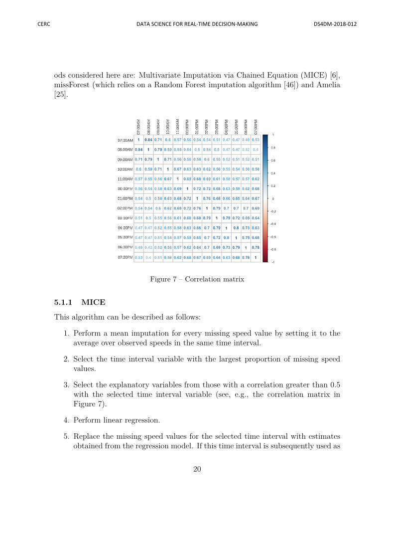
Figure 7 – Correlation matrix

5.1.1 MICE

This algorithm can be described as follows:

1. Perform a mean imputation for every missing speed value by setting it to theaverage over observed speeds in the same time interval.

2. Select the time interval variable with the largest proportion of missing speedvalues.

3. Select the explanatory variables from those with a correlation greater than 0.5with the selected time interval variable (see, e.g., the correlation matrix inFigure 7).

4. Perform linear regression.

5. Replace the missing speed values for the selected time interval with estimatesobtained from the regression model. If this time interval is subsequently used as

20


an explanatory variable in the regression model of other time interval variables,both observed and imputed values are used.

6. Repeat steps 2 to 4 for each remaining time interval with missing values (cyclingthrough each variable stands for one iteration).

7. Repeat the entire procedure for a number of iterations to obtain multiple esti-mates.

At the end, the multiple estimates obtained over the iterations are averaged toobtain a single estimate for each missing value.

5.1.2 Random Forest

The Random Forest (RF) algorithm [5] is a machine learning technique that does notrequire the specification of a particular regression model. It has a built-in routine tohandle missing values by weighting the observed values of a variable using a matrixof proximity values, where proximity is defined by the proportion of trees in whichpairs of observations share a terminal node. It works as follows:

1. Replace missing values by the average over observed values in the same timeinterval.

2. Repeat until a stopping criterion is satisfied:

(a) Using imputed values calculated so far, train a random forest.(b) Compute the proximity matrix.(c) Using proximity as a weight, impute missing values as the weighted average

over observed values in the same time interval.

Typically, the algorithm stops when the difference between the new imputed valuesand the old ones increases for the first time. Note that, by averaging over multiplerandom trees, this method implicitly behaves according to a multiple imputationscheme. The RF algorithm was implemented using the randomForest R-package [30].

5.1.3 Amelia

Amelia imputes missing data based on different bootstrapped samples drawn fromthe database (bootstrapped data samples are large numbers of smaller samples of thesame size that are repeatedly drawn, with replacement, from a single original sample,see [12]). It basically applies the Expectation Maximization (EM) method [11] to findthe maximum likelihood estimates for the parameters of a distribution. Namely,

21


1. M samples are drawn from the original database.

2. M estimates of the mean and variance are calculated for each sample with EM.

3. Each estimate of the mean and variance is used to impute the missing data.

At the end, we have M different complete databases, where the missing values ineach database have been filled with one of the M estimates of the mean and variance.

Each complete database produced by MICE, RF and Amelia is used to providetarget outputs during the training and testing phases of our neural network model.The accuracy of the travel speed predictions made by the neural network will becompared for the three imputation methods considered.

5.2 LSTMIn this section, we briefly describe the supervised neural network model used to predicttravel speeds, once the missing values in the database have been replaced by imputedones (either using MICE, RF or Amelia). The neural network model is a Long Short-Term Memory network (LSTM). This choice was motivated by the ability of theLSTM to handle sequential data and to capture time dependencies. First introducedin [24], this special type of Recurrent Neural Network (RNN) alleviates the vanishinggradient problem [35] (when the gradient of the error function becomes too small withrespect to a given weight, the latter cannot change anymore). It is made of an inputlayer, a variable number of hidden layers and an output layer. Each hidden layer ismade of memory cells that store useful information from past input data. Memorycells in a given hidden layer send signals at time t to the memory cells in the nexthidden layer (or the units in the output layer, if last) but also to themselves. Thisrecurrent signal is used by the memory cells to determine their internal state at timet + 1. Thus, there are connection weight matrices from the input to the first hiddenlayer, from each hidden layer to itself and to the next hidden layer and from thelast hidden layer to itself and to the output layer. Furthermore, memory cells in agiven layer have three gates: one for the signal sent from the previous layer, one forthe signal sent by the memory cells to themselves and one for the signal sent by thememory cells to the next layer. Gates can be seen as filters that regulate the signalsby allowing some parts of it to be blocked (or forgotten). Like the weight matricesmentioned above, the gates have weights that are updated during the learning process.The interested reader will find more details about the LSTM network model in [19].

In the next section, computational results obtained with LSTM and comparisonswith alternative approaches are reported.

22


6 Computational studyIn this section, we first define the input and output vectors of the LSTM. Then, wedescribe the fine tuning of the LSTM hyperparameters. Finally, LSTM results arereported.

Our LSTM was implemented in Python 3.5. The hyperparameter tuning experi-ment was performed on a Dell R630 server with two Intel Xeon E5-2650V4 of 12 coreseach (plus hyperthreading) and 256GB of memory. The server also has 4 NVIDIATitan XP GPUs with 3840 CUDA cores and 12GB of memory. However, our codewas limited to only 4 cores and one GPU from the server. To obtain more computa-tion power, the final LSTM results reported in Sections 6.3 and 6.4 were obtained onthe Cedar cluster of Compute Canada. We requested 6 cores with Intel E5-2650v4processors, 32GB of RAM and 1 NVIDIA P100 GPU with 12GB of memory.

6.1 Input and output vectorsThe input vector for the neural network was first designed as illustrated in Figure 8.Each vector is associated with a class of arcs produced by AP and is made of: theclass label, the day (Monday, Tuesday, ..., Saturday, Sunday), the season (Spring,Summer, Fall, Winter) and 13 average speeds over all arcs in the corresponding class,that is, one speed value for each one-hour time interval starting from 7:00 AM to 7:00PM. The target output vector corresponds to a speed pattern among the 6,667,459available speed patterns, where the missing values are filled with one of the threeimputation methods of Section 5.1. Obviously, the target output vector must comefrom an arc of the same class, and for the same season and day than the vectorprovided in input. We should also note that the speed values in the patterns werenormalized using the scikit-learn object [36].

classlabel day season 07:00AM ........ 07:00PM

13 speed valuesFigure 8 – Input vector I

Unfortunately, the results obtained with this approach were unsatisfactory. Tobetter exploit the capabilities of LSTM to handle sequential data, we turned to inputvector II shown in Figure 9. Here, input vector I with 13 speed values is transformedinto 13 input vectors II, each with a single speed value. That is, rather than providingat once the whole speed pattern for one-hour time intervals starting from 7:00 AM

23


to 7:00 PM, a sequence of 13 input vectors from 7:00 AM to 7:00 PM is provided,where each input vector contains a single speed value. The target output vector ismodified accordingly and also contains a single speed value taken from an arc of thesame class, and for the same season, day and hour than the vector provided in input.

classlabel day season xx:00

one speed valueFigure 9 – Input vector II

6.2 Hyperparameter tuningOur database of 6,667,459 speed patterns was divided into a training set (80% ofthe total) and a testing set (20% of the total), where the latter is made of the mostrecent observations. Apart from the connection weights, which are adjusted throughlearning, a neural network model also relies on a number of other parameters (whereparameter is taken in a broad sense) that must be set before learning takes place.The following were considered:

• Number of hidden layers;

• Number of units in each hidden layer;

• Batch size: Number of training examples provided to the neural network beforeupdating the connection weights;

• Training epochs: Number of passes through the set of training examples;

• Learning algorithm: Algorithm used during the training phase to adjust theweights;

• Weight initialization: Method used to set the initial weights, see [17] for moredetails;

• Activation function: Function used to compute the internal state of a unit fromthe signal it receives.

A good parameter setting for a neural network has a huge impact on its results,as discussed in [2]. To determine an appropriate combination of the above parame-ters, different hyperparameter optimization strategies can be used [45], in particular

24


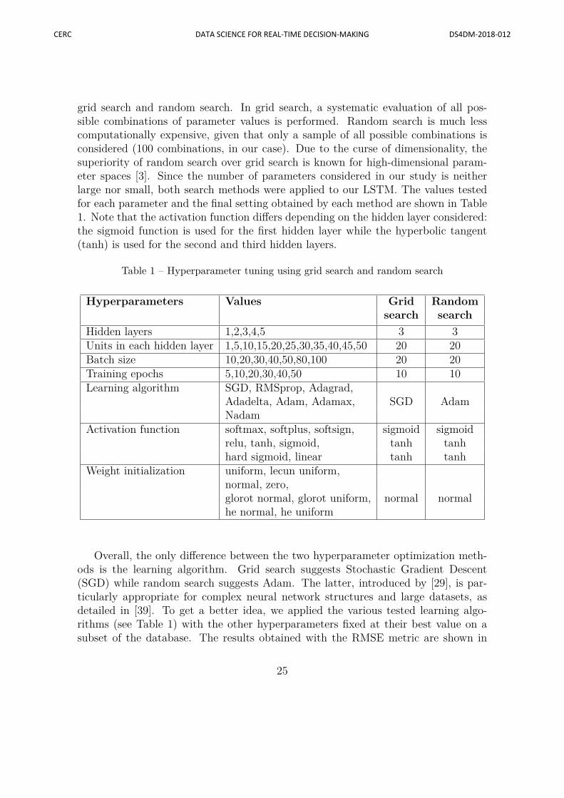
grid search and random search. In grid search, a systematic evaluation of all pos-sible combinations of parameter values is performed. Random search is much lesscomputationally expensive, given that only a sample of all possible combinations isconsidered (100 combinations, in our case). Due to the curse of dimensionality, thesuperiority of random search over grid search is known for high-dimensional param-eter spaces [3]. Since the number of parameters considered in our study is neitherlarge nor small, both search methods were applied to our LSTM. The values testedfor each parameter and the final setting obtained by each method are shown in Table1. Note that the activation function differs depending on the hidden layer considered:the sigmoid function is used for the first hidden layer while the hyperbolic tangent(tanh) is used for the second and third hidden layers.

Table 1 – Hyperparameter tuning using grid search and random search

Hyperparameters Values Grid Randomsearch search

Hidden layers 1,2,3,4,5 3 3Units in each hidden layer 1,5,10,15,20,25,30,35,40,45,50 20 20Batch size 10,20,30,40,50,80,100 20 20Training epochs 5,10,20,30,40,50 10 10Learning algorithm SGD, RMSprop, Adagrad,

Adadelta, Adam, Adamax, SGD AdamNadam

Activation function softmax, softplus, softsign, sigmoid sigmoidrelu, tanh, sigmoid, tanh tanhhard sigmoid, linear tanh tanh

Weight initialization uniform, lecun uniform,normal, zero,glorot normal, glorot uniform, normal normalhe normal, he uniform

Overall, the only difference between the two hyperparameter optimization meth-ods is the learning algorithm. Grid search suggests Stochastic Gradient Descent(SGD) while random search suggests Adam. The latter, introduced by [29], is par-ticularly appropriate for complex neural network structures and large datasets, asdetailed in [39]. To get a better idea, we applied the various tested learning algo-rithms (see Table 1) with the other hyperparameters fixed at their best value on asubset of the database. The results obtained with the RMSE metric are shown in

25


Figure 10. Based on this preliminary experiment, we decided to go with Adam.

Figure 10 – Initial comparison of different learning algorithms

6.3 LSTM resultsHere, we measure the accuracy of the travel speed predictions produced by our LSTMwith three hidden layers. We also compare the results obtained with the three impu-tation methods of Section 5.1 to fill the missing values.

The root mean squared error and the mean absolute error are used to measurethe accuracy, where:

RMSE =

√√√√ 1L

L∑l=1

(yl − yl)2 , (13)

MAE = 1L

L∑l=1|yl − yl| . (14)

In these equations, L is the number of (input, target output) pairs in the trainingor testing set, where the target output corresponds to an observed speed pattern.In pair l, yl stands for the observed speed pattern and yl for the speed patternproduced by the neural network for input vector l. RMSE and MAE are two errorfunctions typically used to evaluate how close the output vectors produced by the

26


neural network are to the target outputs. Due to the square in the RMSE formula,large errors have much more impact than small ones. On the other hand, MAEmeasures the relative error and is more robust to outliers since there is no square inits formula.

Table 2 reports the prediction errors of the trained LSTM on the testing set, basedon the RMSE and MAE metrics, using the three different imputation methods anda variable number of imputations (i.e., 5, 10, 15, 20). Note that the authors in [41]show that 3 to 5 imputations yield good results. But, more recently, the authors in[18, 40] proposed 20 imputations. Thus, we chose to vary this number between 5 and20.

Table 2 – RMSE and MAE metrics with different imputation methods

Method #Imput. MAE RMSE Running

time (min)MICE 5 13.71 12.91 429

10 12.84 10.84 45015 12.52 10.32 111720 12.39 10.09 1900

RF 5 13.84 13.28 51210 13.02 11.38 64915 12.94 11.08 164020 12.68 11.03 2000

AMELIA 5 17.91 17.53 55010 17.63 16.97 58015 16.76 16.10 94020 16.49 16.07 1500

The results show that MICE produces the best results. Although the two errormetrics keep improving with the number of imputations, most of the improvementoccurs between 5 and 10 imputations. Concerning the computing times, a substantialincrease is observed between 10 and 15 imputations for all methods. Overall, MICEis the least computationally expensive for 5, 10 and 15 imputations. The marginalimprovement obtained with 15 and 20 imputations probably does not justify theadditional computational cost. Thus, MICE-10 seems to be a good compromise.

Figure 11 summarizes the evolution of the MAE and RMSE metrics for LSTMwith MICE-10 over a number of training epochs. We can see that RMSE drops soonerthan MAE and then keeps improving at about the same pace than MAE. Figure 12then illustrates the differences between the observed speeds and the speeds predicted

27


by the trained LSTM on the training and testing (input, target output) pairs on asample of observations. This figure shows that, in most cases, the predicted speedvalues follow closely the observed ones.

Figure 11 – Evolution of MAE and RMSE during the training phase

Figure 12 – Comparison between observed and predicted speed values

28


6.4 Comparison with other modelsIn this section, LSTM is compared with two alternative approaches based on a trivialaverage method and a Multi-Layer Perceptron (MLP) trained with the Levenberg-Marquardt algorithm [47]. We tested MLP models with one to three hidden layers,using a variable number of units in the hidden layers. At the end, the error metrics ofthe various models were quite close, although a model with three hidden layers and30 units in each hidden layer proved to be the best. Thus, we only report the resultsfor the best MLP model in Tables 3 and 4.

The average method is quite simple: if we consider an input vector of type I (II)for a given class, day and season (and hour), the output is the average speed pattern(value) over speed patterns (values) of arcs in the same class, for the same day andseason (and hour). The results obtained with the LSTM, MLP and average methodare reported in Tables 3 and 4 using the RMSE and MAE metrics, respectively. Theresults for the two input structures are also reported to show the superiority of inputvector II over input vector I, see Section 6.1. Overall, LSTM clearly provides a betterprediction accuracy than the two other models for both the RMSE and MAE metrics.

Table 3 – Comparison of alternative models: RMSE metric

Model Input vector I Input vector IILSTM 17.22 10.84MLP 21.92 15.17Average 38.04 32.04

Table 4 – Comparison of alternative models: MAE metric

Model Input vector I Input vector IILSTM 22.86 12.84MLP 29.57 17.40Average 42.62 36.98

7 ConclusionIn this work, a “prediction-after-classification” approach was proposed, starting froma large database of GPS traces collected from mobile devices installed inside delivery

29


vehicles. We used dimensionality reduction and unsupervised learning techniques toextract similarity classes of arcs to be used during the following supervised predictionphase.

Because supervised learning algorithms are sensitive to missing values, differentmultiple imputation methods were applied to obtain a complete database. The pre-diction problem was addressed with a LSTM neural network whose parameters wereadjusted with random search. The LSTM was then compared to two alternativemodels and prove to be largely superior.

A natural extension of the work reported in this paper would be to include real-time data in the prediction process. The ultimate goal is to integrate the currentpredictor into a vehicle routing optimization procedure to produce more efficientdelivery routes.

Acknowledgments. Financial support was provided by the Natural Sciences and Engi-neering Research Council of Canada through the Canada Excellence Research Chairin Data Science for Real-Time Decision-Making. Also, computing facilities were madeavailable to us by Compute Canada. This support is gratefully acknowledged. Fi-nally, we wish to thank Prof. Leandro C. Coelho and his team for their contributionto the analysis of the GPS data.

References[1] C. Antoniou, M. Ben-Akiva, and H.N. Koutsopoulos. Nonlinear Kalman filtering

algorithms for on-line calibration of dynamic traffic assignment models. IEEETransactions on Intelligent Transportation Systems, 8(4):661–670, 2007.

[2] J. Bergstra, R. Bardenet, Y. Bengio, and B. Kegl. Algorithms for hyper-parameter optimization. In J. Shawe-Taylor, R.S. Zemel, P.L. Bartlett,F. Pereira, and K.Q. Weinberger, editors, Advances in Neural Information Pro-cessing Systems 24, pages 2546–2554. Curran Associates, Inc., 2011.

[3] J. Bergstra and Y. Bengio. Random search for hyper-parameter optimization.Journal of Machine Learning Research, 13:281–305, 2012.

[4] George EP Box and Gwilym M Jenkins. Time series analysis: forecasting andcontrol, revised ed. Holden-Day, 1976.

[5] L. Breiman. Random forests. Machine Learning, 45(1):5–32, 2001.

[6] S. Buuren and K. Groothuis-Oudshoorn. MICE: Multivariate imputation bychained equations in R. Journal of Statistical Software, 45(3), 2011.

30


[7] T. Calinski and J. Harabasz. A dendrite method for cluster analysis. Commu-nications in Statistics, 3(1):1–27, 1974.

[8] H. Chen, S. Grant-Muller, L. Mussone, and F. Montgomery. A study of hybridneural network approaches and the effects of missing data on traffic forecasting.Neural Computing & Applications, 10(3):277–286, 2001.

[9] K. Cho, B. Van Merrienboer, C. Gulcehre, D. Bahdanau, F. Bougares,H. Schwenk, and Y. Bengio. Learning phrase representations using RNN encoder-decoder for statistical machine translation. arXiv preprint arXiv:1406.1078,2014.

[10] G.A. Davis and N.L. Nihan. Nonparametric regression and short-term freewaytraffic forecasting. Journal of Transportation Engineering, 117(2):178–188, 1991.

[11] A.P. Dempster, N.M. Laird, and D.B. Rubin. Maximum likelihood from incom-plete data via the EM algorithm. Journal of the Royal Statistical Society. SeriesB, pages 1–38, 1977.

[12] B. Efron and R.J. Tibshirani. An introduction to the bootstrap. CRC press, 1994.

[13] A. Ermagun and D. Levinson. Spatiotemporal traffic forecasting: Review andproposed directions. Transport Reviews, pages 1–29, 2018.

[14] B.J. Frey and D. Dueck. Clustering by passing messages between data points.Science, 315(5814):972–976, 2007.

[15] R. Fu, Z. Zhang, and L. Li. Using LSTM and GRU neural network methodsfor traffic flow prediction. In Youth Academic Annual Conference of the ChineseAssociation of Automation, pages 324–328. IEEE, 2016.

[16] K. Fukunaga and L. Hostetler. The estimation of the gradient of a density func-tion, with applications in pattern recognition. IEEE Transactions on InformationTheory, 21(1):32–40, 1975.

[17] X. Glorot and Y. Bengio. Understanding the difficulty of training deep feedfor-ward neural networks. In Proceedings of the Thirteenth International Conferenceon Artificial Intelligence and Statistics, pages 249–256, 2010.

[18] J.W. Graham, A.E. Olchowski, and T.D. Gilreath. How many imputations arereally needed? Some practical clarifications of multiple imputation theory. Pre-vention Science, 8(3):206–213, 2007.

31


[19] K. Greff, R.K. Srivastava, J. Koutnık, B.R. Steunebrink, and J. Schmidhhuber.LSTM: A search space odyssey. IEEE Trans. on Neural Networks and LearningSystems, 28(10):2222–2232, 2017.

[20] J. Guo. Adaptive Estimation and Prediction of Univariate Vehicular TrafficCondition Series. Ph.D. Thesis, North Carolina State University, 2005.

[21] A.B. Habtie, A. Abraham, and D. Midekso. Artificial neural network basedreal-time urban road traffic state estimation framework. In Computational In-telligence in Wireless Sensor Networks, pages 73–97. Springer, 2017.

[22] M.M. Hamed, H.R. Al-Masaeid, and Z.M.B. Said. Short-term prediction of trafficvolume in urban arterials. Journal of Transportation Engineering, 121(3):249–254, 1995.

[23] M. Hashemi and H.A. Karimi. A weight-based map-matching algorithm for vehi-cle navigation in complex urban networks. Journal of Intelligent TransportationSystems, 20(6):573–590, 2016.

[24] S. Hochreiter and J. Schmidhuber. Long short-term memory. Neural Computa-tion, 9(8):1735–1780, 1997.

[25] J. Honaker, G. King, and M. Blackwell. Amelia II: A program for missing data.Journal of Statistical Software, 45(7):1–47, 2011.

[26] H. Jula, M. Dessouky, and P.A. Ioannou. Real-time estimation of travel timesalong the arcs and arrival times at the nodes of dynamic stochastic networks.IEEE Transactions on Intelligent Transportation Systems, 9(1):97–110, 2008.

[27] S.J. Julier and J.K. Uhlmann. New extension of the Kalman filter to nonlinearsystems. In AeroSense’97, pages 182–193. International Society for Optics andPhotonics, 1997.

[28] R.E. Kalman and R.S. Bucy. New results in linear filtering and prediction theory.Journal of Basic Engineering, 83(1):95–108, 1961.

[29] D.P. Kingma and J. Ba. Adam: A method for stochastic optimization. arXivpreprint arXiv:1412.6980, 2014.

[30] A. Liaw and M. Wiener. Classification and regression by randomforest. R news,2(3):18–22, 2002.

[31] R.J.A. Little and D.B. Rubin. Statistical Analysis with Missing Data. JohnWiley & Sons, 2014.

32


[32] X. Ma, Z. Tao, Y.i Wang, H. Yu, and Y. Wang. Long short-term memoryneural network for traffic speed prediction using remote microwave sensor data.Transportation Research Part C: Emerging Technologies, 54:187–197, 2015.

[33] J. MacQueen. Some methods for classification and analysis of multivariate obser-vations. In Proceedings of the Fifth Berkeley Symposium on Mathematical Statis-tics and Probability, volume 1, pages 281–297. University of California Press,1967.

[34] M. Moniruzzaman, H. Maoh, and W. Anderson. Short-term prediction of bordercrossing time and traffic volume for commercial trucks: A case study for theAmbassador bridge. Transportation Research Part C: Emerging Technologies,63:182–194, 2016.

[35] R. Pascanu, T. Mikolov, and Y. Bengio. On the difficulty of training recurrentneural networks. In International Conference on Machine Learning, pages 1310–1318, 2013.

[36] F. Pedregosa, G. Varoquaux, A. Gramfort, V. Michel, B. Thirion, O. Grisel,M. Blondel, P. Prettenhofer, R. Weiss, V. Dubourg, J. Vanderplas, A. Passos,D. Cournapeau, M. Brucher, M. Perrot, and E. Duchesnay. Scikit-learn: Machinelearning in Python. Journal of Machine Learning Research, 12:2825–2830, 2011.

[37] P.J. Rousseeuw. Silhouettes: A graphical aid to the interpretation and validationof cluster analysis. Journal of Computational and Applied Mathematics, 20:53–65, 1987.

[38] D.B. Rubin. Multiple Imputation for Nonresponse in Surveys. John Wiley &Sons, 2004.

[39] S. Ruder. An overview of gradient descent optimization algorithms. arXivpreprint arXiv:1609.04747, 2016.

[40] J.L. Schafer and J.W. Graham. Missing data: our view of the state of the art.Psychological Methods, 7(2):147, 2002.

[41] J.L. Schafer and M.K. Olsen. Multiple imputation for multivariate missing-data problems: A data analyst’s perspective. Multivariate Behavioral Research,33(4):545–571, 1998.

[42] B.L. Smith. Forecasting Freeway Traffic Flow for Intelligent Transportation Sys-tems Application. PhD thesis, Charlottesville, VA, USA, 1995.

33


[43] B.L. Smith and M.J. Demetsky. Traffic flow forecasting: comparison of modelingapproaches. Journal of Transportation Engineering, 123(4):261–266, 1997.

[44] B.L. Smith, B.M. Williams, and R.K. Oswald. Comparison of parametric andnonparametric models for traffic flow forecasting. Transportation Research PartC: Emerging Technologies, 10(4):303–321, 2002.

[45] J. Snoek, H. Larochelle, and R.P. Adams. Practical Bayesian optimization ofmachine learning algorithms. In Advances in Neural Information ProcessingSystems, pages 2951–2959, 2012.

[46] D.J. Stekhoven and P. Buhlmann. Missforest-Non-parametric missing value im-putation for mixed-type data. Bioinformatics, 28(1):112–118, 2011.

[47] I. Sutskever. Training Recurrent Neural Networks. Ph D. Thesis, University ofToronto, Toronto, Canada, 2013.

[48] Y. Tian and L. Pan. Predicting short-term traffic flow by long short-termmemory recurrent neural network. In IEEE International Conference on SmartCity/SocialCom/SustainCom (SmartCity), pages 153–158. IEEE, 2015.

[49] C.P. Van Hinsbergen, J.W. Van Lint, and F.M. Sanders. Short term trafficprediction models. In Proceedings of the 14th World Congress on IntelligentTransportation Systems (ITS), Bejing, China, 2007.

[50] J.W.C. Van Lint. Online learning solutions for freeway travel time prediction.IEEE Transactions on Intelligent Transportation Systems, 9(1):38–47, 2008.

[51] V.N. Vapnik. An overview of statistical learning theory. IEEE Transactions onNeural Networks, 10(5):988–999, 1999.

[52] V.N. Vladimir. The Nature of Statistical Learning Theory. Springer Heidelberg,1995.

[53] E. Vlahogianni, M. G Karlaftis, and J.C. Golias. Optimized and meta-optimizedneural networks for short-term traffic flow prediction: A genetic approach. Trans-portation Research Part C: Emerging Technologies, 13(3):211–234, 2005.

[54] J. Wang and Q. Shi. Short-term traffic speed forecasting hybrid model based onchaos–wavelet analysis-support vector machine theory. Transportation ResearchPart C: Emerging Technologies, 27:219–232, 2013.

34


[55] Y. Wang and M. Papageorgiou. Real-time freeway traffic state estimation basedon extended Kalman filter: A general approach. Transportation Research PartB: Methodological, 39(2):141–167, 2005.

[56] B.M. Williams and L.A. Hoel. Modeling and forecasting vehicular traffic flow asa seasonal ARIMA process: Theoretical basis and empirical results. Journal ofTransportation Engineering, 129(6):664–672, 2003.

[57] C.-H. Wu, J.-M. Ho, and D.-T. Lee. Travel-time prediction with support vectorregression. IEEE Transactions on Intelligent Transportation Systems, 5(4):276–281, 2004.

[58] Z. Yang, D. Mei, Q. Yang, H. Zhou, and X. Li. Traffic flow prediction model forlarge-scale road network based on cloud computing. Mathematical Problems inEngineering, Volume 2014, 2014.

35


Date post:	29-Jan-2022
Category:	Documents
Upload:	others
View:	7 times
Download:	0 times

TRAVEL SPEED PREDICTION BASED ON LEARNING METHODS …

Documents