trophic structure of mesopelagic fishes over cold seeps in the north central gulf of mexico

TROPHIC STRUCTURE OF MIDWATER FISHES OVER COLD SEEPS IN THE NORTH CENTRAL GULF OF MEXICO

Jennifer P. McClain-Counts

A Thesis Submitted to the University of North Carolina Wilmington in Partial Fulfillment

of the Requirements for the Degree of Master of Science

Center for Marine Science

University of North Carolina Wilmington

2010

Approved by

Advisory Committee

Steve W. Ross Lawrence B. Cahoon Chair

Joan W. Willey

Accepted by

Dean, Graduate School

TABLE OF CONTENTS ABSTRACT....................................................................................................................... iv

ACKNOWLEDGMENTS ................................................................................................. vi

DEDICATION.................................................................................................................. vii

LIST OF TABLES........................................................................................................... viii

LIST OF FIGURES ........................................................................................................... xi

INTRODUCTION ...............................................................................................................1

METHODS ..........................................................................................................................4

Study Area ................................................................................................................4

Sample Collection ....................................................................................................5

Dietary Analyses ......................................................................................................6

Gut Content Analyses ...................................................................................6

Stable Isotope Analyses ................................................................................7

IsoSource Mixing Model ............................................................................10

Trophic Position Analyses......................................................................................10

Statistical Analyses.................................................................................................11

RESULTS ..........................................................................................................................13

Catch Data ..............................................................................................................13

Gut Content Analyses.............................................................................................13

Diet composition .........................................................................................13

Factors influencing diet composition ..........................................................17

Stable Isotope Analyses..........................................................................................19

Trophic Position Calculations ................................................................................23

ii

DISCUSSION....................................................................................................................24

Diet composition ....................................................................................................24

Spatial and Temporal influences on diet ................................................................30

Additional insight with SIA....................................................................................32

Site differences............................................................................................32

Diet variations .............................................................................................33

Methodology...........................................................................................................34

Interesting Note ......................................................................................................35

CONCLUSIONS................................................................................................................36

LITERATURE CITED ......................................................................................................37

iii

ABSTRACT

Midwater fishes are an important component of pelagic food webs and provide insight into

energy utilization and movement through the water column. In this study, the diets of midwater

fishes collected over cold seep habitats were examined to determine general feeding patterns and

whether size, depth, time of day or location affected diet composition within fish species. The

base of the midwater food web was also examined to determine whether chemosynthetic energy

in benthic cold seeps was incorporated into the midwater fish community. Discrete depth Tucker

trawling was conducted in August 2007 over three cold seep habitats (> 1000 m) in the north-

central Gulf of Mexico. Surface sampling was also conducted to provide a prey base

(zooplankton and POM) for stable isotope analyses (SIA). Gut content analysis (GCA) and SIA

(δ13C and δ15N) in conjunction with IsoSource software were utilized for diet reconstruction and

to determine trophic positions. SIA also aided efforts to determine chemosynthetic influences on

the midwater food web. GCA was performed on 31 species in the five most abundant families

(Gonostomatidae, Myctophidae, Phosichthyidae, Sternoptychidae and Stomiidae), with midwater

fishes classified into one of three guilds: piscivore, large crustacean consumer, or

zooplanktivore. SIA was performed on 6 fish families (Gonostomatidae, Myctophidae,

Phosichthyidae, Sternoptychidae, Stomiidae, and Melamphaidae), 13 invertebrate categories, and

3 primary producers (POM, Sargassum spp. and detritus), and classified all fishes as

zooplanktivores. Using IsoSource, more precise contributions of individual prey taxon were

documented, which did not always support results from GCA. Size, depth, time of day and

location did not affect diet composition within a species; however migration trends suggested

competition may be reduced by feeding over a range of depths and over a 24 hour period.

Significant differences in trophic position calculations between GCA and SIA highlighted the

iv

importance of using multiple techniques to describe trophic structure, as each method

characterized the diets differently.

v

ACKNOWLEDGMENTS

This project was largely funded by the Department of the Interior U.S. Geological Survey

under Cooperative Agreement No. 05HQAG0009, sub agreement 05099HS004. I thank the crew

of the R/V Cape Hatteras and all scientific personal for assisting with fishing operations and

sample processing. S. Artabane, A. Quattrini, and A. Roa-Varon assisted with fish

identifications and C. Ames assisted with invertebrate identifications. Guidance and support

during stable isotope analyses were provided by Drs. A. Demopoulos and C. Tobias, and K.

Duernberger. I would also like to thank S. Artabane, T. Casazza and A. Roa-Varón for their

assistance in dissecting and processing fish stomachs. Special thanks to my committee, Drs. S.

Ross, L. Cahoon, and J. Willey, for their guidance and support during the duration of this project.

I would additionally like to thank my advisor, Dr. S. Ross, for setting me up with this project and

Dr. L. Cahoon for his assistance with statistics. Finally, thanks to S. Ross, T. Casazza, A.

Demopoulos, A. Quattrini, L. Truxal and M. Carlson for their suggestions and edits provided

throughout the writing process of this thesis.

vi

DEDICATION

I would like to dedicate this thesis to my parents, who encouraged my early passion in

marine science and gave me the confidence to follow my dreams and overcome any obstacles.

Your constant love and support was unwavering and because of that, I can present this Masters

project.

vii

LIST OF TABLES

Table Page 1. Surface and midwater stations sampled over three cold seep sites

(AT340, GC852, and AC601) (see Fig.1) in the Gulf of Mexico (9-25 August 2007)................................................................................................48

2. The total number of all midwater fishes, invertebrates and

autotrophs examined in dietary analyses from the North-central Gulf of Mexico ......................................................................................................55

3. Results of ANOSIM comparing effects of size, time of day, depth

and location on the general prey categories consumed for each fish species.............................................................................................................58

4. Percent volume and frequency of prey items consumed by

Chauliodus sloani collected from three sites in the Gulf of Mexico (AC601, GC852, AT340) separated by time of day..............................................59


Gonostoma elongatum collected from three sites in the Gulf of Mexico (AC601, GC852, AT340) separated by time of day ................................60


Stomiidae collected from three sites in the Gulf of Mexico (AC601, GC852, AT340) separated by time of day..............................................62


Cyclothone alba collected from three sites in the Gulf of Mexico (AC601, GC852, AT340) separated by time of day..............................................63


Cyclothone braueri collected from three sites in the Gulf of Mexico (AC601, GC852, AT340) separated by time of day ................................65


Cyclothone pseudopallida collected from three sites in the Gulf of Mexico (AC601, GC852, AT340) separated by time of day ................................66


Hygophum benoiti collected from three sites in the Gulf of Mexico (AC601, GC852, AT340) separated by time of day ............................68

viii

11. Percent volume and frequency of prey items consumed by Valenciennellus tripunctulatus collected from three sites in the Gulf of Mexico (AC601, GC852, AT340) separated by time of day....................69


Diaphus mollis collected from three sites in the Gulf of Mexico (AC601, GC852, AT340) separated by time of day..............................................71


Cyclothone pallida collected from three sites in the Gulf of Mexico (AC601, GC852, AT340) separated by time of day..............................................73


Vinciguerria poweria collected from three sites in the Gulf of Mexico (AC601, GC852, AT340) separated by time of day ................................74


Myctophum affine collected from three sites in the Gulf of Mexico (AC601, GC852, AT340) separated by time of day ................................77


Argyropelecus aculeatus collected from three sites in the Gulf of Mexico (AC601, GC852, AT340) separated by time of day ................................79

17. Percent volume and frequency of prey items consumed by Argyropelecus hemigymnus collected from three sites in the Gulf of Mexico (AC601, GC852, AT340) separated by time of day ............................81

18. Percent volume and frequency of prey items consumed by Pollichthys mauli collected from three sites in the Gulf of Mexico (AC601, GC852, AT340) separated by time of day ................................82


Benthosema suborbitale collected from three sites in the Gulf of Mexico (AC601, GC852, AT340) separated by time of day..............................................84


Lampanyctus alatus collected from three sites in the Gulf of Mexico (AC601, GC852, AT340) separated by time of day ................................86


Lepidophanes guentheri collected from three sites in the Gulf of Mexico (AC601, GC852, AT340) separated by time of day..............................................88

ix

22. Percent volume and frequency of prey items consumed by Notolychnus valdiviae collected from three sites in the Gulf of Mexico (AC601, GC852, AT340) separated by time of day ................................90

23. Percent volume and frequency of prey items consumed by Ceratoscopelus warmingii collected from three sites in the Gulf of Mexico (AC601, GC852, AT340) separated by time of day ............................92

24. Mean (± 1 SE) δ13C and δ15N values for midwater fishes, invertebrates

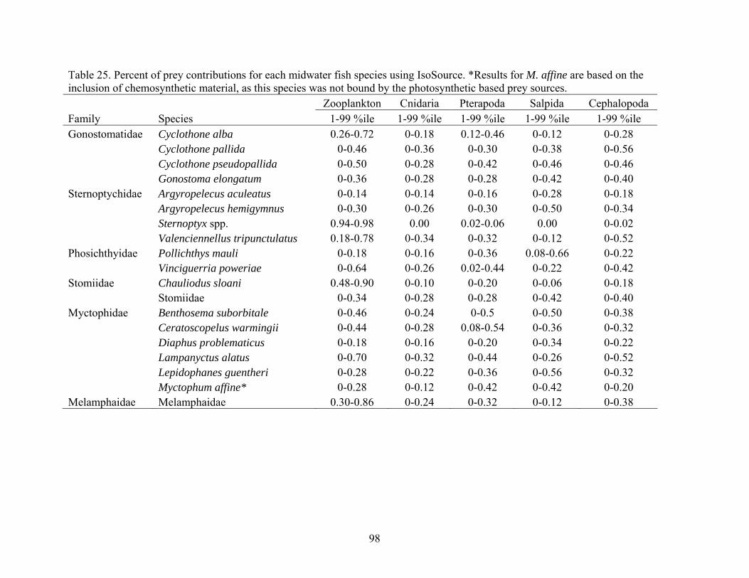
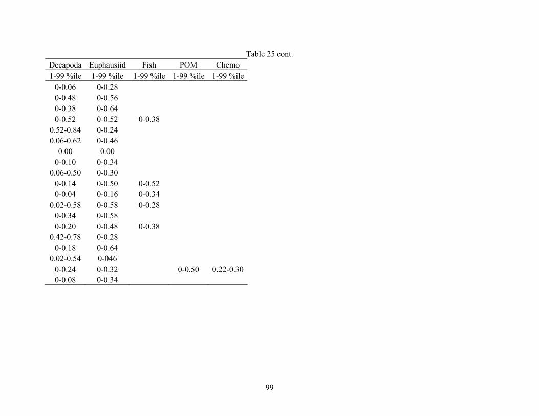
and carbon sources collected from each site (AC601, AT340, GC852) ...............95 25. Percent of prey contributions for each midwater fish species using

IsoSource ...............................................................................................................98 26. Mean trophic position (TP), one standard deviation (SD), range

(minimum – maximum) and number of fish (n) for each midwater fish species collected in the North-central Gulf of Mexico, using data from stable isotope and gut content analyses ......................................................100

x

LIST OF FIGURES

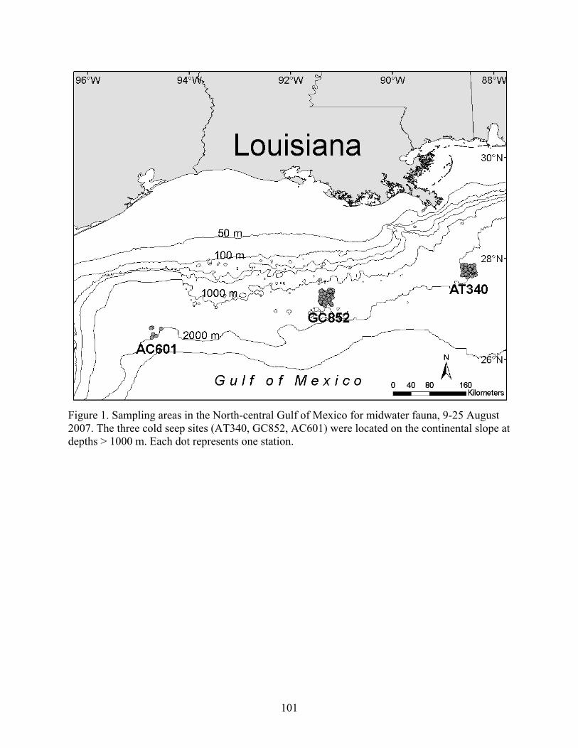
Figure Page 1. Sampling areas in the North-central Gulf of Mexico for midwater

fauna, 9-25 August 2007. The three cold seep sites (AT340, GC852, AC601) were located on the continental slope at depths > 1000 m. Each dot represents one station ...........................................................................101

2. Multidimensional scaling (MDS) plot documenting the differences

among the gut contents of midwater fishes. Data were based on the Bray-Curtis similarity matrix calculated from standardized, square root transformed, mean volumes of prey (12 general categories) .......................102

3. Relationships among stomach fullness, mean depth of capture and

time for midwater fishes. Data were compiled from all sites and excluded specimens lacking depth data...............................................................103

4. Plot of the average δ15N values against the average δ13C values

(± 1 standard error) for midwater fishes, invertebrates and primary producers collected in the Gulf of Mexico ..........................................................111

5. Relationship between δ15N and SL for all midwater fish species........................112

xi

INTRODUCTION

Midwater fishes constitute an important component of the pelagic food web due to their high

abundances, migratory behavior, and global distribution (Gjøsaeter and Kawaguchi 1980;

Cornejo and Koppelmann 2006). Many of these unique fishes inhabit the mesopelagic zone (200

to 1000 m), and although they are consumed by a variety of marine fauna, such as benthic

grenadiers (Laptikhovsky 2005), pelagic tuna (Potier et. al. 2007), and penguins (Adams et al.

2004), midwater fishes are also fierce predators. In the eastern Gulf of Mexico, midwater fishes

consume 5-10% of the daily zooplankton production in the epipelagic zone (< 200 m) (Hopkins

et al. 1996). The ability of midwater fishes to impact both surface and bottom communities

results from diel vertical migrations (DVMs), a unique behavior exhibited by many midwater

fish species. Species that undergo DVMs migrate from the mesopelagic zone to the epipelagic

zone at night, primarily at sunset, and return to the mesopelagic zone at sunrise. Through DVMs,

midwater fishes, particularly myctophids (Kinzer 1977; Hidaka et al. 2001; Cornejo and

Koppelmann 2006), contribute significantly to the vertical transport of organic matter from the

epipelagic zone to the mesopelagic zone (Ashjian et al. 2002; Brodeur and Yamamura 2005),

thus impacting the trophic structure of the water column. By tracking these trophic relationships,

a more thorough understanding of pelagic energy and material flow through the water column

can be established.

Previous dietary studies on midwater fishes (Hopkins and Baird 1985a,b; Lancraft et al.

1988; Hopkins et al. 1996; Butler et al. 2001; Pusch et al. 2004) utilized gut content analyses

(GCA) to determine trophic relationships. Generally, midwater fishes were divided into three

major feeding guilds: zooplanktivores, which consume planktonic organisms such as amphipods,

copepods and euphausiids; micronektonivores, which consume fishes and cephalopods; and

1

generalists, which consume a variety of unrelated taxa (Gartner et al. 1997). Unfortunately, as

GCA only represent short-term diet (< 24 hours) (Hadwen et al 2007), placement into these

feeding guilds could vary and may be inaccurate. Guild placement can be affected by dietary

shifts resulting from changes in prey abundance (Kawaguchi and Mauchline 1982), seasonality

(Kawaguchi and Mauchline 1982) and ontogeny (Kawaguchi and Mauchline 1982; Young and

Blaber 1986; Hopkins et al. 1996; Beamish et al. 1999; Williams et al. 2001; Butler et al. 2001).

Additionally, accurate guild placement is not possible for specimens with empty stomachs,

common in midwater fishes (Gartner et al. 1997). The trophic relationships relating midwater

fishes to their carbon sources are also limited with GCA, which may not always allow the

determination of which autotrophs contributed to a food web (Thomas and Cahoon 1993).

Therefore, despite providing detailed dietary data, GCA only documents a portion of the trophic

structure.

Issues related to GCA (noted above) may be addressed using stable isotope analyses (SIA).

Although SIA cannot provide detailed prey data (e.g., species level prey identifications), SIA

provides general information on the cumulative feeding habits of an organism (Fry 2006).

Trophic positions within a food web (Fry 1988; Van Dover 2000; Hobson 2002; Behringer and

Butler 2006; Fry 2006; Paradis et al. 2008) can be estimated from SIA due to the isotopic ratio of

nitrogen (15N/14N or δ15N), increasing an average of 3.4‰ per trophic level (Minagawa and

Wada 1984; Post 2002). In contrast to nitrogen, the isotopic ratio of carbon (13C/12C or δ13C), has

little fractionation between trophic levels, with an increase ≤ 1‰ per trophic level (Post 2002;

Lajtha and Michener 1994; Minagawa and Wada 1984). Despite this low fractionation, carbon is

useful for determining carbon sources as distinct ranges are documented for different autotrophs:

-22 to -16‰ for marine phytoplankton (Post 2002; Fry 2006), -18 to -15‰ for Sargassum spp.

2

(Rooker et al. 2006), -16 to -5‰ for turtlegrass (Hemminga and Mateo 1994), and -75 to -28‰

for chemosynthetic material (Kennicutt et al. 1992). Unfortunately, despite the added benefit of

combining SIA and GCA in dietary analyses, few studies (e.g. Vander Zanden et al. 1997;

Hadwen et al. 2007; Drazen et al. 2008; Rybczynski et al. 2008) have done so.

In the Gulf of Mexico (GOM), trophic structure may be affected by the complex bottom

topography and hydrography. The dominant current, the Loop Current, flows from the Caribbean

Sea through the Yucatan Channel, around the east-central portion of the GOM and flows out near

southern Florida (Hyun and Hogan 2008; Sturges et al. 2005). The oscillation of this current

often results in warm- and cold-core rings breaking off, which affect circulation (Schmitz et al.

2005), primary productivity and food web dynamics (Waite et al. 2007). Additionally, the

Mississippi River flows into the northern portion of the basin providing large amounts of

freshwater, sediments and nutrients, affecting both the water physics and chemistry and faunal

communities (Baguley et al. 2006; Jarosz and Murray 2005). The presence of benthic features,

like cold seeps or corals, can also affect trophic complexity, particularly as chemosynthetic

communities can be associated with cold seeps. Higher abundances of non-seep, benthic fauna

were occasionally observed in the vicinity of seeps (Levin 2005) and may consume

chemosynthetic material (MacAvoy et al. 2002; 2008). However, whether midwater fishes are

impacted by chemosynthetic energy pathways either in the water column above the seep areas or

by interactions with the associated benthic communities has not been examined.

Food web studies provide an effective means of tracking energy flow through an ecosystem.

The purpose of this study was to examine the trophic structure of midwater fishes over cold seep

areas (> 1000 m) in the north-central GOM. The presence of changing hydrography and prey

resources at the sites may affect trophic structure. This study used both GCA and SIA to

3

thoroughly document the trophic relationships of midwater fishes. The objectives were to: 1)

determine basic feeding patterns of the dominant midwater fish species collected, 2) document

feeding changes, if any, that occurred among species due to differences in size, time of day,

depth or location, 3) examine the relationship, if any, between feeding and DVM patterns in the

midwater fishes, 4) document the differences in short term (GCA) and long term (SIA) feeding,

and 5) examine the base of the midwater food web to determine whether the midwater

community utilized chemosynthetic energy sources from cold seeps.

METHODS

Study Area

Three cold seep sites in the GOM were selected for sampling based on data collected by TDI-

Brooks International, Inc: Atwater Valley Block 340 (AT340), Green Canyon Block 852

(GC852), and Alaminos Canyon Block 601 (AC601). These three sites are located on the middle

to lower continental slope in the north-central GOM, and each contained benthic chemosynthetic

communities (Fig. 1). Detailed bottom topography was documented for each site from previous

seismic profiles and surveys from a submersible and a remotely operated vehicle (Roberts et al.

2007). AT340 (2216 m) contained multiple mounds located on a topographic high. Submersible

surveys of the area documented extensive carbonate substrata, large mussel beds, clumps of

tubeworms and a few soft corals. GC852 (1450 m) was characterized by an elongated ridge

approximately 2 km long running north to south, with vast amounts of carbonate substrata and

numerous corals on the crest. Tubeworms and mussel beds were also documented at this site.

Additionally, oil slicks were present on the surface and bubble streams were reported on the

bottom, which may be potential mechanisms for transporting benthic material to the surface.

AC601 (2340 m) differed from the other two sites, having low topography and a large brine pool.

4

Some carbonate substrata and a few isolated aggregations of tubeworms were present, none of

which were near the brine pool. High methane concentrations in the water column were also

recorded in the water column over this site (Roberts et al. 2007).

Sample Collection

Intense sampling of the upper 1000 m of the water column was conducted during 24 hour

operations at all three sites from 9-25 August 2007; however, due to inclement weather, only

minimal night sampling was conducted at AC601. A total of 173 stations (45 day, 108 night, and

20 twilight) were sampled (Table 1). Multiple gear types were utilized to adequately sample the

fauna, including a Tucker trawl, Neuston net, and plankton nets, though discrete-depth Tucker

trawling was emphasized. Midwater fauna were collected using a Tucker trawl (2 x 2 m, 1.59

mm mesh, 505 μm cod end.) with a plankton net (0.5 m diameter, 335 μm mesh) attached inside

the Tucker trawl mouth to simultaneously sample the smaller components of the midwater fauna.

Trawls were equipped with a Sea-Bird SBE39 temperature-depth recorder (TDR) attached to the

upper frame bar to record time, depth, and temperature during deployment. The Tucker trawl

was deployed open, and it was assumed no significant fishing occurred during deployment due to

the rapid lowering, steep wire angle, and minimal forward movement of the vessel (Gartner et

al., 2008; Ross et al. 2010). Upon reaching the designated depth, the trawl fished for

approximately 30 min at a 2 knot (3.7 km/hr) ground speed and was triggered closed using a

double trip mechanism. Actual time and depth fished for each trawl was determined post-tow

using data from the TDR. TDR data were used throughout the cruise to adjust fishing strategies

to achieve desired sampling depths. The mean depth for each Tucker trawl tow was calculated by

averaging all depths recorded by the TDR from the start to the end of each tow. Tucker trawling

5

intensely sampled the upper 1000 m of the water column over the 24 hour time period at GC852

and AT340.

Zooplankton samples were collected from a 1.1 x 2.4-m Neuston net (6.4-mm mesh body and

3.2-mm tail bag) or plankton nets (0.5 m diameter, 335 μm and 1.0 m diameter, 505 μm mesh)

deployed at the surface and towed for 15-30 minutes (Table 8.1). Particulate organic material

(POM) was collected by filtering seawater through a 125-μm precombusted glass filter, and it

was assumed that the majority of POM was phytoplankton derived (Kling et al., 1992). POM and

zooplankton samples provided a food web base for SIA.

Fishes collected were preserved in 10% seawater-formalin solution and later transferred to

50% isopropyl for storage until dietary analyses. Invertebrates were preserved in 70% ethanol,

with the exception of jelly and salp specimens that were preserved in 10% seawater-formalin

solution. All specimens were sorted, identified to the lowest possible taxa and measured to the

nearest millimeter standard length (SL) (fishes) or total length (TL) (invertebrates). The life

history stage of fishes was also documented based on the presence or absence of gonads. Fish

specimens were classified as juvenile when either no gonads or immature gonads were present.

Dietary Analyses

Gut Content Analysis (GCA)

GCA was conducted for the five most abundant midwater families (31 species) using

methods outlined in Ross and Moser (1995). All abundant species collected (> 30 individuals,

with the exception of stomiids) were analyzed. In order to increase sample size for Stomiidae, all

stomiids, with the exception of C. sloani, were grouped together and were collectively referred to

as Stomiidae. Highly abundant fish species, Cyclothone alba (n = 614), C. braueri (n = 669), C.

pallida (n = 885), C. pseudopallida (n = 744), Valenciennellus tripunctulatus (n = 248), and

6

Notolychnus valdiviae (n = 1139), were randomly subsampled, with selected specimens spanning

the collected size range of the species, encompassing all depths sampled, and including day,

night and twilight samples. Selected fishes were dissected and the stomachs were removed.

Stomach fullness was estimated as 0%, 5%, 25%, 50%, 75% or 100%. Empty stomachs were

documented, though not included in most analyses, for day, night and twilight samples at all

sites. Stomach contents were placed on a Petri dish and identified to the lowest possible taxon.

Similar prey items were then piled together on a grid of 1 mm squares and flattened to a uniform

height, which was measured. This height multiplied by the number of squares occupied by the

food item yielded volume in mm3. The frequency of occurrence for a prey item equaled the

number of times a prey item occurred in the fish species examined divided by the total number of

stomachs analyzed.

The relationship between DVMs and stomach fullness was examined by plotting stomach

fullness against time of day and mean sampling depth. Time of day was divided into three

categories: day (0730 to 1830 hr CDT), night (2030 to 0530 hr CDT), and twilight (0530 to 0730

hr CDT, one hour on either side of average sunrise, and 1830 to 2030 hr CDT, one hour on either

side of average sunset) and mean sampling depths were calculated based on Ross et al. (2010).

TT tows where no mean sampling depth was calculated were excluded.

Stable Isotope Analysis (SIA)

Prior to specimen preservation in formalin or ethanol, samples of white muscle tissue were

dissected from fishes and invertebrates and frozen. For consistency, tissue was removed from

similar body regions based on the type of specimen (i.e., muscle tissue removed from the dorsal

region of fishes, the caudal region of shrimps, the legs of crabs and the mantle of mollusks).

When specimens were too small to extract a tissue sample, the whole body was used. Minimal

contamination from other tissue types occurred as the head, scales, photophores, and entrails

7

were removed from specimens taken whole. For these specimens, species identification was

made either prior to tissue collection, or a replicate specimen was vouchered for future

identification. All collected isotope samples were dried and crushed into a powder. The majority

of samples were dried to a constant weight in an oven at 50-60˚C. Additional samples were

frozen at -80˚C for ≥ 24 hours and freeze dried in a VirTis Benchtop 3.3 Vac-Freeze. I assumed

there were no significant differences in isotopic ratios as a result of different drying techniques

(Bosley and Wainright 1999).

Tissue samples were analyzed for carbon and nitrogen isotope ratios. For each sample, 400-

600 μg were placed into a tin capsule and combusted in an Elemental Combustion System Model

4010 coupled to a Delta V Plus Isotope Ratio Mass Spectrometer (IRMS) via Conflo II interface

at the University of North Carolina Wilmington (UNCW). POM (provided by A. Demopoulos,

USGS), 49 fishes and 24 invertebrates were analyzed by IRMS at Washington State University

using a Costech (Valencia, USA) elemental analyzer interfaced to a GV instruments

(Manchester, UK) Isoprime IRMS. Precision of the IRMS at UNCW was verified by repeated

analysis of standards USGS 40 and USGS 41, which were incorporated into each sample run.

Raw delta values were corrected for linearity and normalized to known reference materials

USGS 40 and USGS 41. A similar procedure was utilized at Washington State University using

egg albumin powder calibrated against National Institute of Standards reference materials.

Reproducibility was monitored using several organic reference standards (Fry 2007). Isotope

ratios were expressed in the standard delta (δ) notation as parts per thousand (‰) according to

the following equation:

1000*R

)R - (R X

standard

standardsample=δ (1)

8

where X is 13C or 15N and R is the corresponding ratio 13C/12C or 15N/14N. The global standards

for δ13C and δ15N are Vienna PeeDee Belemnite and atmospheric nitrogen (air). A minimum of 5

samples were analyzed per fish species. Similar to GCA, the sample size of Stomiidae was

increased by combining all species, with the exception of C. sloani. Similarly, 3 melamphid

species (Melamphaes simus, M. typhlops, and Scopelogadus mizolepis) were grouped together to

increase sample size for analyses and were referred to as Melamphaidae. Diaphus spp. included

D. mollis and D. lucidus and Sternoptyx spp. included S. diaphana and S. pseudobscura.

Data were examined after SIA to determine whether inorganic carbon or lipids may have

significantly impacted the isotope results. According to Post et al. (2007) samples with C:N > 4

are likely affected by the presence of lipids, and inorganic carbon may be present when C:N >

3.5 or δ13C is highly enriched. Our results (all C:N < 4) indicated that neither lipids nor inorganic

carbon significantly impacted the isotope ratios of fishes; therefore, no lipid extraction or

acidification methods were utilized for fish isotope samples. In contrast, some invertebrates had

high C:N values that suggested the presence of inorganic carbon in the samples. As a result, an

acidification process was conducted on a subset of invertebrate samples, which included

amphipods, copepods, euphausiids, jellyfish, pterapods, salps, and zooplankton, to remove any

inorganic carbon. To acidify samples, 1.0 N hydrochloric acid was added one drop at a time to

dried, crushed tissue samples until bubbling no longer occurred. Acidified samples were air dried

for 8 hours before being re-dried in an oven at 50-60˚C for 24 hours. These samples were then

processed by the same method utilized for nonacidifed samples (see above). As acidification can

affect N values, acidified samples were reported with δ15N reflecting the ratio from the untreated

sample and δ13C reflecting the acidified sample (Jacob et al. 2005; Pinnegar and Polunin 1999).

9

Isotope Mixing Models

Isotope data were analyzed using IsoSource 3.5. IsoSource is a multisource mixing model

program that calculates all possible solutions for the contribution of each prey source to a

consumer’s diet based on the isotopic signatures of the prey and predator (Phillips and Gregg

2003; Benstead et al. 2006). For this study, the average carbon and nitrogen values for each prey

item and fish were entered into the mixing model to determine all feasible contributions. Prior to

analysis, nitrogen values for consumers were corrected for trophic fractionation, set at 2‰, based

on the trophic shift documented in my isotope data. It was assumed no trophic fractionation

occurred in carbon (Demopoulos et al. 2007; France and Peters 1997). Tolerance was set at 0.2%

with source increments set at 0.2%. Reported ranges represented the 1-99th percentile because

the resulting ranges (minimum to maximum) are sensitive to small numbers of observations at

the ends of the distribution and the 1-99th percentile range may be more robust to outliers

(Philips and Gregg 2003).

Trophic position analysis

Data collected during GCA and SIA were used to calculate the trophic position of each

individual fish based on the following two equations from Vander Zanden et al. (1997)

[ ]∑ += 1))(( iiGC TPVTP (2)

where TPGC is the trophic position of the fish based on gut content analysis, Vi is the percent

volume of a nth prey item and TPi is the trophic position of nth prey item based on data from

Rybczynski et al. (2008) and

2)(

)( 11515

+−

= °

fNN

TP consumerfishSIA

δδ (3)

10

where TPSIA is the trophic position of the fish based on stable isotope analysis and f is the trophic

fraction for one trophic level.

Statistical Analyses

Multivariate analyses were conducted on gut contents of each fish species to examine diet

differences based on four factors: size, time of day, depth and location. All analyses utilized the

software PRIMER-E version 6.1 (Clarke and Warwick 2001; Clarke and Gorley 2006). Factors

were divided into groups as follows: SL was divided into size classes based on 5 mm increments

(10-14 mm, 15-19 mm, 20-24 mm, 25-29 mm, 30-34 mm, 35-39 mm, 40-44 mm, 45-49 mm, 50-

54 mm, 55-59 mm, 60-64 mm, 65-69 mm, 70-74 mm, 75-79 mm, 80-84 mm, 85-89 mm, 90-94

mm, 95-99 mm, 100-104 mm, 105-109 mm, 110-114 mm, ≥115 mm); time of day was divided

into three categories, day (0730 to 1830 hr CDT), night (2030 to 0530 hr CDT), and twilight

(0530 to 0730 and 1830 to 2030 hr CTD); depth (based on mean sample depth) was divided into

ranges based on 50 m increments (surface-49 m, 50-99 m, 100-149 m, 150-199 m, 200-249 m,

250-299 m, 300-349 m, 350-399 m, 400-449 m, 450-499 m, 500-549 m, 550-599 m, 600-649 m,

650-699 m, 700-749 m, 850-899 m, 900-949 m, 950-999 m, 1000-1049 m, 1050-1099 m, 1100-

1149 m, 1150-1199 m); and location was divided into the three sites (AT340, GC852, AC601).

Organic material and animal parts (e.g., amphipod parts, copepod parts, decapod parts) were

excluded prior to analyses as these food items were ambiguous and may be pieces of prey items

identified to lower taxa. For each fish species, the prey item volumetric data were standardized

for each individual fish by dividing the volume of each prey item by the total volume of the

stomach in order to account for stomach fullness variability. Standardized volumes were then

square root transformed to down weight the contributions of abundant prey items. Next,

similarities among fish species were calculated using a Bray-Curtis similarity coefficient based

11

on each factor. The resulting similarity matrix was then subjected to a one way analysis of

similarities (ANOSIM) to determine if diets were significantly different for each factor, with

R>0.40 and p<0.05 used as the criteria for statistical significance. When significant differences

were found using ANOSIM, a similarity percentages routine (SIMPER) was utilized to

determine which prey items contributed to the dissimilarities. This process was repeated for each

fish species.

A similar multivariate procedure was implemented for diet comparisons among all 31 fish

species, disregarding the factors size, time of day, depth and location. After constructing a Bray-

Curtis similarity matrix, results were subjected to hierarchical clustering with group average

linkage and non-metric multidimensional scaling (MDS). With a large sample size (n = 1327), a

MDS plot can become cluttered with substantial “noise” in individual samples; therefore, data

were averaged by PRIMER based on species prior to standardization (see above for

standardization process) (Clarke and Gorley 2006). Additionally, to determine general feeding

guilds, all fish species were analyzed using general prey categories (Amphipoda, Annelida,

Chaetognatha, Cnidaria, Copepoda, Crustacea, Decapoda, Euphausiacea, Fish, Mollusca,

Ostracoda, Salpida, and Other). For this analysis, identifiable animal parts were included in the

general categories (i.e., copepod parts were included in Copepoda), but organic material and

unidentifiable animal parts (e.g., crustacean parts, animal parts) were excluded. Clusters were

defined at the 30% and 60% similarity levels.

Statistical analyses were conducted on isotope ratios and trophic-level calculations using

SigmaStat 3.4. Data were analyzed for normality and homogeneity of variance using

Kolmogorov-Smirnov and Levene Median tests. One-way analysis of variance (ANOVA) was

used to determine significant differences in isotopic values for primary producers, invertebrates

12

and fishes, with the exception of Phosichthyidae, where a t-test was used to determine

differences between P. mauli and V. poweriae. A post-hoc Tukey test was used to determine

specific differences among groups. Data that failed normality or equal variance tests were

analyzed with ANOVA on the Ranks and the post-hoc Dunn’s test. Species comparisons

between sites AT340 and GC852 were analyzed using a two-way ANOVA and post-hoc Holm-

Sidak test. An ANOVA on the Ranks, followed by Dunn’s test, was used to determine significant

differences in the trophic position based on GCA or SIA. Trophic positions calculated from GCA

were compared to trophic positions calculated from SIA using a t-test; however, data that failed

normality were analyzed using a Mann-Whitney rank sum test. Species with low sample sizes (n

< 5) were not analyzed statistically. Regressions of δ15N against fish SL were conducted to

determine whether ontogenetic shifts in diet occurred. Statistical significance was determined

when p < 0.05. Isotope data were reported with the mean ± 1 standard error.

RESULTS

Catch data

Tucker trawling consisted of 123 tows (33 day and 90 night) from three sites (AT340,

GC852, and AC601); however, minimal sampling (n = 5, night only) was conducted at AC601.

The mean depth ranges sampled were: 63 to 1503 m for AT340, 21 to 1067 m for GC852, and 45

to 584 m for AC601. A total of 8,716 fishes (30 families) were collected, but 97.7% of these

fishes were from five midwater fish families: Gonostomatidae (58.8%), Myctophidae (27.4%),

Phosichthyidae (5.8%), Sternoptychidae (4.4%) and Stomiidae (1.3%).

Gut Content Analyses (GCA)

Diet composition

GCA were conducted on 31 species from the five most abundant midwater fish families

13

(Table 2). Gut contents were analyzed from 2,989 fishes, of which 1,658 (55%) stomachs were

empty. A total of 125 prey items (45 species, 37 families) were identified in the stomachs of all

midwater fishes, and items were grouped into 13 general prey taxa: Amphipoda, Annelida,

Chaetognatha, Cnidaria, Copepoda, Crustacea, Decapoda, Euphausiacea, Fish, Mollusca,

Ostracoda, Salpida, and Other. Copepods were the dominant prey, identified in 79% of stomachs

and were consumed by all species except C. sloani. The MDS ordination plot of mean prey

volumes for the 31 midwater fish species defined three general feeding guilds at a 30% similarity

level (Fig. 2): piscivores, large crustacean consumers, and zooplanktivores. At a 60% similarity,

the piscivore guild remained unchanged, but the large crustacean consumer guild was subdivided

into two subguilds, decapod-euphausiid consumer and decapod-piscivore, and the zooplanktivore

guild was subdivided into three subguilds, copepod consumer, mixed zooplanktivore, and a

generalist consumer (Fig. 2).

The piscivore guild contained only one species, C. sloani (Fig. 2). Empty stomachs occurred

in over 80% of all stomachs analyzed (Table 4). Within stomachs that contained food, six prey

items (3 prey categories) were identified. Myctophidae and Bregmaceros spp. were the most

important prey items in overall percent volume and frequency, and no identifiable invertebrates

were documented (Table 4).

Large crustacean consumers consisted of G. elongatum and Stomiidae (Fig. 2). Decapods

were the dominant prey item, comprising over 70% of the identifiable prey volume of this guild.

At 60% similarity, this guild was divided into two subguilds: decapod-euphausiid consumer and

decapod-piscivore consumer. The decapod-euphausiid consumer subguild contained one species,

G. elongatum. Empty stomachs, all from night collections, occurred in 24% of analyzed G.

elongatum (Table 5). This species had 29 prey items (9 prey categories) identified (Table 5), and

14

while decapods and euphausiids were important prey volumetrically, copepods, particularly

calanoid, were consumed more frequently (Table 5). The decapod-piscivore consumer subguild

was comprised of Stomiidae. Empty stomachs occurred more frequently in this subguild and

were documented in 69% of all stomiids (Table 6). The diet of Stomiidae was less variable than

G. elongatum and was characterized by 11 prey items (4 prey categories) identified in the

stomachs. Decapods and myctophids were the most important prey in overall percent volume and

frequency for Stomiidae (Table 6).

All other midwater fishes were classified as zooplanktivores, which was divided into three

subguilds. The copepod consumer subguild contained C. alba, C. braueri, C. pseudopallida, V.

tripunctulatus, D. mollis, and H. benoiti. Copepods comprised over 90% of the diet (Fig. 2). A

high percentage (> 68%) of empty stomachs occurred in C. alba (Table 7), C. braueri (Table 8),

C. pseudopallida (Table 9), and H. benoiti (Table 12), while fewer empty stomachs were

documented in V. tripunctulatus (17%, Table 10) and D. mollis (9%, Table 11). Although

Copepoda was the major prey category consumed in terms of volume and frequency, stomachs

contained a diversity of prey (Tables 7-12), ranging from 13 prey items for H. benoiti (Table 10)

to 36 prey items for V. tripunctulatus (Table 11). Pleuromamma spp. was the dominant copepod

in terms of volume and frequency consumed by C. alba (Table 7), V. tripunctulatus (Table 11),

and D. mollis (Table 12), whereas Aegisthus mucronatus was more important in the diets of C.

braueri (Table 8). Valdiviella minor was volumetrically more important in the diet of C.

pseudopallida, but Lubbockia spp. occurred more frequently (Table 9). Calanoid copepods were

volumetrically important in the diets of H. benoiti, but cyclopoid copepods occurred more

frequently (Table 10).

15

The mixed zooplanktivores subguild was defined by a general crustacean diet, with species

consuming a variety of zooplankton. This subguild contained C. pallida, A. aculeatus, A.

hemigymnus, P. mauli, V. poweriae, B. suborbitale, L. alatus, L. guentheri, M. affine, and N.

valdiviae (Figure 2). The presence of empty stomachs was variable in this subguild, ranging from

21% of specimens containing empty stomachs (L. alatus) to 94% of specimens containing empty

stomachs (C. pallida). Examination of gut contents revealed the overall diet diversity for mixed

zooplanktivores was greater than copepod consumers, ranging from 10 prey items for C. pallida

(Table 13) to 42 prey items for V. poweriae (Table 14). Amphipoda was more important

volumetrically in the diet of C. pallida (Table 13) and M. affine (Table 15), while Conchoecinae

(Ostracoda) was more important for A. aculeatus (Table 16) and A. hemigymnus (Table 17).

Ostracods, particularly Conchoecinae, also occurred frequently in the stomachs of C. pallida

(Table 13), A. aculeatus (Table 16), and P. mauli (Table 18), while calanoid copepods

(particularly Pleuromamma spp.) occurred more frequently in the stomachs of M. affine (Table

15), A. hemigymnus (Table 17), B. suborbitale (Table 19), L. alatus (Table 20), L. guentheri

(Table 21) and N. valdiviae (Table 22). Similar to copepod consumers, Pleuromamma spp. and

other calanoid copepods were important prey items for P. mauli (Table 18), B. suborbitale

(Table 19), L. alatus (Table 20), L. guentheri (Table 21) and N. valdiviae (Table 22); however

decapods, euphausiids and ostracods also influenced their diets volumetrically. Vinciguerria

poweriae exhibited a more unique diet compared to other mixed zooplanktivores, with

myctophids and Candaciidae (Copepoda) dominating the diet volumetrically, but Conchoecinae

and calanoid copepods occurring more frequently (Table 14).

The generalist subguild contained only C. warmingii. This fish had the most variable diet of

any zooplanktivore, with more non-crustacean prey consumed than any other zooplanktivore.

16

Empty stomachs occurred in 18% of C. warmingii, while stomach contents revealed a total of 39

prey items (13 categories, Table 23). Crustaceans comprised roughly 60% of the identifiable diet

and non-crustacean prey comprised about 40% (Table 23). Fish, molluscs, and copepods were

more important in overall percent volume of the diet, though copepods occurred more frequently

than any other prey item (Table 23).

Factors influencing diet composition

Variations in diet composition due to size differences were investigated using GCA. The size

range was reported for each fish species (Table 2). No significant differences in diet composition

were documented based on size within species (Table 3), although the majority (79%) of fishes

analyzed were juveniles.

Gut contents were analyzed to determine whether time affected diet composition.

Statistically, similar prey was consumed by midwater fish species regardless of the time of day

(Table 3); however, some general trends were documented in regards to the prevalence of empty

stomachs. Empty stomachs occurred more frequently during the day (0730-1830) in C. sloani

(Tables 4), C. pallida (Tables 13), V. poweriae (Tables 14), M. affine (Tables 15), P. mauli

(Tables 18), B. suborbitale (Tables 19), L. alatus (Tables 20), and C. warmingii (Tables 23),

while empty stomachs occurred more frequently in the day and twilight (0730-2030) in C. alba

(Tables 7), C. braueri (Tables 8), C. pseudopallida (Tables 9), H. benoiti (Tables 10), V.

tripunctulatus (Tables 11), and D. mollis (Table 12). For G. elongatum (Tables 5), Stomiidae

(Tables 6), A. aculeatus (Tables 16), A. hemigymnus (Tables 17) and L. guentheri (Tables 21),

empty stomachs were documented more frequently in specimens collected at night (2030-0530),

and more specimens of N. valdiviae with empty stomachs were collected at twilight (0530-0730

and 1830-2030, Table 22).

17

Diet composition was examined on horizontal and vertical spatial scales in addition to

temporal scales. Comparisons among sites yielded no significant differences in diet composition

(Table 3). There was also no significant difference in diet composition based on depth, with the

exception of A. hemigymnus (ANOSIM, R = 0.546, p = 0.019). SIMPER analysis documented an

average dissimilarity of 59.3% for A. hemigymnus collected between 400-449 m compared to

450-499 m. Ostracoda (32.8%), Copepoda (32.1%) and Euphausiacea (29.2%) contributed to the

diet dissimilarity between these depths, with less diet variability (copepods only) documented in

the stomachs of specimens collected between 400-449 m.

Despite the lack of significant differences temporally and spatially, migration patterns were

examined to document general trends in feeding. No DVMs were documented for C. alba or C.

braueri (Figure 3A-B), with more full stomachs documented at night (2030-0530) in the mid

mesopelagic range (350 – 700 m). DVMs were slightly evident for C. pallida, C. pseudopallida,

A. hemigymnus, and V. tripunctulatus (Figure 3C-F), with more full stomachs documented

during the day (0730-1830) in the lower mesopelagic (700 – 1100 m) for C. pallida (Figure 3C),

more full stomachs documented at night (2030-0530) in the mid mesopelagic range (350 – 700

m) for A. hemigymnus (Figure 3E) and V. tripunctulatus (Figure 3F), and C. pseudopallida

consuming prey during a 24 hour period (Figure 3D). For species that underwent DVMs, G.

elongatum, A. aculeatus, P. mauli, V. poweriae, B. suborbitale, C. warmingii, D. mollis, H.

benoiti, L. alatus, L. guentheri, and N. valdiviae (Fig. 3G-Q), fuller stomachs occurred more

frequently at night in the epipelagic/upper mesopelagic (surface to 350 m). Myctophum affine

deviated from this pattern in migrating midwater fishes, with fuller stomachs occurring more

frequently at night in the mid mesopelagic (Fig. 3R). Stomiids were another exception, with C.

sloani having more full stomachs at night in the mid mesopelagic (350 – 700 m, Fig. 3S) and

18

Stomiidae having more full stomachs during the day in the lower mesopelagic (700 – 1100 m,

Fig. 3T).

Stable isotope analyses (SIA)

SIA were conducted on 337 samples, collected from the Neuston net (n = 1), plankton nets (n

= 41), TT (n = 274), and filtered seawater (n= 21). These samples represented 30 fish species (6

families), 10 general invertebrate taxa (Amphipoda, Cephalopoda, Chaetognatha, Cnidaria,

Copeopda, Decapoda, Euphausicea, Gastropoda, Salpida, Zooplankton) and three potential

carbon sources (detritus, Sargassum spp., and POM, Table 2).

Spatial variations in δ13C and δ15N were examined for fishes, invertebrates and carbon

sources (Table 24). No statistical comparisons were conducted on detritus (only collected at

AT340), or Sargassum spp. (n < 5 at AC601 and AT340). POM sampling revealed no

significant difference in δ13C among sites; however, samples collected at GCA852 were depleted

in 15N compared to AT340 (post-hoc Tukey test, p = 0.003). Small sample sizes of invertebrates

at each site also prevented statistical spatial comparisons on all invertebrate categories except

Copepoda, Decapoda and Euphausiacea (Table 24). There were no significant differences in 13C

or 15N for Copepoda between sites GC852 and AT340. Neither Decapoda nor Euphausiacea had

any significant differences in 13C between GC852 and AT340; however, both were significantly

enriched in 15N at GC852 compared to AT340 (post-hoc Tukey test, p < 0.001). Spatial

comparisons among fishes collected GC852 and AT340 were also limited by small sample sizes

and only conducted on G. elongatum, A. aculeatus, V. poweriae, and L. alatus. There were no

significant differences in δ13C within any fish species collected at GC852 or AT340. Nitrogen

was significantly enriched in G. elongatum and L. alatus collected at GC852 compared to

specimens collected at AT340 (Holm-Sidak, unadjusted p < 0.001, unadjusted p = 0.008), while

19

A. aculeatus was depleted in 15N at GC852 compared to AT340 (Holm-Sidak, unadjusted p =

0.049) and V. poweriae had no significant differences in δ15N between GC852 and AT340.

Valenciennellus tripunctulatus, the only fish species statistically analyzed at all three sites, was

significantly enriched in 13C at AT340 compared to V. tripunctulatus collected at GC852 and

AC601 (Tukey, p = 0.018); however, there were no significant differences in δ15N among sites.

Data were also compared across sites to evaluate non-spatial species differences in isotopes.

There was a clear distinction in δ13C for each of the three carbon sources. Detritus was

significantly enriched in 13C compared to POM (Tukey, p < 0.001) and Sargassum spp. (Tukey,

p < 0.001), while Sargassum spp. was significantly enriched in 13C compared to POM (Tukey, p

= 0.031). There were no significant differences in δ15N between detritus and Sargassum spp. or

detritus and POM; however, Sargassum spp. was significantly depleted in 15N compared to POM

(Dunn’s, p < 0.05).

Examination of non-spatial differences in isotopes among invertebrate taxa was also

conducted; however, most specimens were grouped into general taxa categories due to small

sample sizes. Both δ15N and δ13C were similar among invertebrates with the following

exceptions. Salpida was depleted in 15N compared to all other invertebrates, although this

difference was only significant compared to Chaetognatha, Gennadas valens, Acanthephyra

purpurea, and Copepoda (all comparisons, Dunn’s, p < 0.05). Also, Acanthephyra purpurea and

Systellaspis debilis were both significantly enriched in 13C compared to Chaetognatha,

Copepoda, and Zooplankton (all comparisons, Dunn’s, p < 0.05). Comparisons among three

decapod species, Gennadas valens, Acanthephyra purpurea, and Systellaspis debilis, revealed

that G. valens was significantly depleted in 13C compared to A. purpurea (Tukey, p = 0.02), and

20

S. debilis (Tukey, p = 0.02), and A. purpurea were significantly enriched in 15N compared to S.

debilis (Dunn’s, p < 0.05).

Similarly, non-spatial differences in δ13C and δ15N were examined among midwater fish

families and species. No significant differences in δ13C existed among the 6 fish families;

however, Sternoptychidae was significantly enriched in 15N compared to Phosichthyidae and

Myctophidae (Dunn’s, p < 0.05). Additional differences were documented among individual

species within each family as follows. In Gonostomatidae, there were no significant differences

in δ13C; however, C. pallida was significantly enriched in 15N compared to C. alba and C.

pseudopallida (Dunn’s, p < 0.05). In Sternoptychidae, A. aculeatus and A. hemigymnus were

enriched in 13C compared to Sternoptyx spp. and V. tripunctulatus (all comparisons, Tukey, p <

0.05), while V. tripunctulatus was significantly enriched in 15N compared to A. hemigymnus

(Dunn’s, p < 0.05). Between phosichthyid species, V. poweriae was significantly enriched in 15N,

but depleted in 13C compared to P. mauli (t-test, p < 0.001). All stomiid species exhibited similar

isotopic signatures, with no significant differences in δ15N or δ13C. Among myctophid species,

M. affine was significantly depleted in 13C compared to all other myctophids (Tukey, p < 0.05)

and was also depleted in 15N, though differences were only significant when compared to

Diaphus spp., D. problematicus, and L. alatus (all comparisons, Dunn’s, p < 0.05). Diaphus spp.

was significantly enriched in 15N compared to C. warmingii (Dunn’s, p < 0.05) and D.

problematicus was enriched in 13C compared to L. alatus (Tukey, p < 0.05).

SIA also indicated trophic relationships within the mesopelagic food web. Enrichment in 15N

was evident with increasing trophic levels, with a trophic fractionation of roughly 2‰, while

trophic fractionation in δ13C was less apparent (Fig. 4). No distinct chemosynthetic signature

(δ13C ranging from -75 to -28‰) was detected in any flora or fauna, with the δ13C values for all

21

fishes reported within the range of photosynthetic-based material. The first trophic level,

representing the base of the mesopelagic food web, was comprised of POM (Fig. 4). The second

trophic level, identified after applying a 2‰ trophic fractionation to POM, contained mostly

zooplankton, such as Copepoda, Euphausiacea, and Amphipoda (Fig. 4). The third trophic level,

designated by a second 2‰ trophic enrichment, encompassed the majority of mesopelagic fishes

(Fig. 4), with one exception (M. affine), which was depleted in both 15N and 13C, relegating it to

the second trophic level.

IsoSource was used to calculate the potential contribution of each prey category to the

midwater fishes (Table 25). Crustaceans were the dominant prey and were reported in the diets

of all midwater fishes. Zooplankton was an important prey item for C. alba, Sternoptyx spp., V.

tripunctulatus, C. sloani, and Melamphaidae, with potential contributions ranging from 18-98%

of their diets. For A. aculeatus, A. hemigymnus, P. mauli, Stomiidae, D. problematicus, and L.

guentheri, Decapoda was an important prey item, with potential contributions ranging from 2-

84%. Non-crustacean prey items, such as Pterapoda, had contributions ranging from 2-54% of

the diets of C. alba, Sternoptyx spp., V. poweriae, P. mauli, and C. warmingii, while Salpida had

contributions ranging from 8-66% of the diet for P. mauli. In some cases, such as C. pallida, C.

pseudopallida, G. elongatum, B. suborbitale and L. alatus, it was not possible to determine prey

contributions to the diets with confidence. The lack of confidence in determining prey

contributions stemmed from all prey sources having a minimal contribution of zero to the diets,

with these fishes not confined within the isotopic signatures of the prey items analyzed in

IsoSource. Myctophum affine deviated from all other midwater fishes, with no solutions

generated for diet contribution based on the zooplankton and POM analyzed due to the depleted

13C reported; however, solutions were generated when the average isotopic signature of

22

chemosynthetic material (based on published literature) was included in the IsoSource analysis.

Minimal contributions of chemosynthetic material ranged from 22-30% of the diet for M. affine;

however, this did not necessarily indicate consumption of chemosynthetic material because

values were based on averages and the isotopic signature of M. affine was within the range of

photosynthetic material.

Ontogenetic shifts were investigated for Cyclothone alba, C. pallida, C. pseudopallida, G.

elongatum, A. aculeatus, A. hemigymnus, Sternoptyx spp., V. tripunctulatus, P. mauli, V.

poweriae, C. sloani, Stomiidae, B. suborbitale, C. warmingii, Diaphus spp., D. problematicus, L.

alatus, L. guentheri, M. affine, and Melamphaidae (Fig 5A-T) by examining the relationships

between δ15N and SL. Positive relationships between δ15N and SL were identified in nineteen of

the twenty species analyzed; however, significant relationships were identified in C.

pseudopallida (R2 = 0.736, p = 0.002), G. elongatum (R2 = 0.618, p = 0.002), V. poweriae (R2 =

0.614, p < 0.001), C. sloani (R2 = 0.852, p = 0.009), D. problematicus (R2 = 0.738, p = 0.013),

Diaphus spp. (R2 = 0.838, p = 0.029) and Melamphaidae (R2 = 0.687, p = 0.003). One significant

negative relationship was also identified in M. affine (Fig. 3S), with lower δ15N documented in

larger individuals (R2 = 0.408, p = 0.047).

Trophic position calculations

Trophic position calculations for the midwater fishes varied by the type of analysis (GCA

versus SIA). Using data from GCA, the calculated trophic positions among fish species ranged

from 2.90 (C. warmingii) to 4.00 (Stomiidae, Table 26). Significant differences among these

trophic positions only occurred between C. sloani and C. braueri (Dunn’s, p < 0.05) and

Stomiidae and C. braueri (Dunn’s, p < 0.05), with the stomiids occupying a higher trophic

position. For isotope data, the calculated trophic positions of midwater fishes had a broader range

23

than those derived from GCA. Trophic positions from SIA ranged from 1.19 (M. affine) to 3.96

(C. pallida), and more significant differences in trophic positions were documented among fish

species. The myctophid M. affine occupied a significantly lower trophic position than C. pallida,

A. aculeatus, Sternoptyx spp., V. tripunctulatus, Diaphus spp., and Melamphaidae, while C.

warmingii occupied a significantly lower trophic position than C. pallida, V. tripunctulatus and

Diaphus spp. (All comparisons, Dunn’s, p < 0.05). Also, P. mauli occupied a significantly lower

trophic position than C. pallida (Dunn’s, p < 0.05), A. aculeatus (Dunn’s, p < 0.05), V.

tripunctulatus (Dunn’s, p < 0.05), and Diaphus spp. (Dunn’s, p < 0.05), while V. tripunctulatus

occupied a significantly higher trophic position than B. suborbitale (Dunn’s, p < 0.05) and L.

guentheri (Dunn’s, p < 0.05). Trophic positions of midwater fishes calculated from SIA data

were significantly lower than trophic positions calculated from gut content data for C. alba

(Mann-Whitney, p < 0.001), C. pseudopallida (p < 0.001), P. mauli (p < 0.001), V. poweriae (p

= 0.025), C. sloani (p < 0.001), Stomiidae (p = 0.022), B. suborbitale (p < 0.001), C. warmingii

(t-test, p < 0.001), L. guentheri (Mann-Whitney, p < 0.001), and M. affine (Mann-Whitney, p <

0.001). In contrast, C. pallida (Mann-Whitney, p = 0.022) and V. tripunctulatus, (p < 0.001)

occupied significantly higher trophic positions according to data from SIA than GCA. There

were no significant differences between trophic positions calculated from GCA and SIA for G.

elongatum, A. aculeatus, A. hemigymnus, Diaphus spp. and L. alatus.

DISCUSSION

Diet Composition

Zooplankton was the dominant prey for midwater fishes. Based on SIA, all species, with the

exception of M. affine, were one trophic level above zooplankton. Additionally, copepods,

particularly Pleuromamma spp., were prevalent in the stomachs of all midwater fishes except C.

24

sloani. This prevalence of zooplankton in the diets of midwater fishes, which was support with

SIA, suggested midwater fishes may be competing for zooplankton prey; however, a more

detailed examination of diet composition using GCA revealed three feeding guilds within

midwater fishes, similar to results from Gartner et al. (1997).

Chauliodus sloani occupied a different guild than all other midwater fishes, with only fishes

documented in the stomachs. Physical adaptations, such as large curved teeth, an expansive oral

cavity and a lack of ossification in the anterior vertebrate, which allow the skull to move upward

and back (Borodulina 1972), make it easier for C. sloani to capture larger prey like myctophids

and Bregmaceros spp. The high number of empty stomachs in C. sloani may indicate that

foraging was not always successful in the epipelagic zone (Sutton and Hopkins 1996; present

study). Sutton (2005) suggested zooplankton may be consumed by C. sloani to sustain energetic

needs between successful feeding on larger prey and crustaceans were previously documented in

the stomachs of C. sloani in the eastern GOM (Hopkins et al. 1996; Sutton and Hopkins 1996),

Arabian Sea (Butler et al. 2001) and off Hawaii (Clarke 1982). IsoSource also supported this

concept of zooplankton consumption, with 48-90% of the diet of C. sloani comprised of

zooplankton. This relationship between foraging success and zooplankton consumption may also

explain ontogenetic diet shifts documented in C. sloani using SIA. Roe and Badcock (1984)

reported that crustaceans, particularly euphausiids, were consumed more by smaller (< 120 mm)

specimens of C. sloani (Roe and Badcock 1984), which were likely less efficient at capturing

fishes. Overall, the incorporation of zooplankton suggested that despite occupying the piscivore

guild, C. sloani may feed more similar to other midwater fishes than previously thought.

Similar to C. sloani, Stomiidae occupied a different guild than the majority of midwater

fishes. Fishes, particularly myctophids, were consumed by Stomiidae, revealing some trophic

25

similarity to C. sloani; however, Stomiidae was classified as a large crustacean consumer due to

the dominance of decapods in the diet. Placement in this guild was further supported by

IsoSource, with decapods comprising 2-58% of the diets. Previous literature documented

decapods, euphausiids and copepods in the stomachs of stomiid species, such as Astronesthes,

Photostomias and Malacosteus; however, other stomiids, such as Idiacanthus and Stomias

consumed fishes, (Clarke 1982; Hopkins et al. 1996; Sutton and Hopkins 1996; Sutton 2005;

present study). Differences in diet composition among stomiid species suggested that guild

classification for Stomiidae was not robust because guild placement for Stomiidae was

dependent on the species grouped together for analyses; therefore, if more piscivorous stomiids

were analyzed in this study, Stomiidae would occupy a niche more similar to C. sloani than G.

elongatum. Even though guild placement was variable, the overall trophic position of Stomiidae

remained unchanged because large crustaceans, such as the decapod G. valens, consumed

zooplankton (Hopkins et al. 1994), similar to myctophids, such as D. mollis; therefore, regardless

of whether Stomiidae consumed fishes or large crustaceans, Stomiidae remained a tertiary

consumer.

Gonostoma elongatum was classified in the same guild as Stomiidae, with decapods

documented as the dominant prey. In addition to consuming large crustaceans, G. elongatum

frequently incorporated smaller zooplankton, such as the copepod Pleuromamma spp., into its

diet. This was similar to previous findings in the eastern GOM (Lancraft et al. 1988; Hopkins et

al. 1996) and was supported by SIA. Clarke (1982) suggested G. elongatum was a

zooplanktivore but it consumed large crustaceans because it reached larger sizes than other

zooplanktivores. This, along with the previously mentioned studies, suggested diets shifted with

ontogeny; however, GCA reported G. elongatum consumed similar prey regardless of size. It

26

was possible that larger G. elongatum consumed similar, but trophically higher prey specimens.

Ontogenetic diet changes were documented in prey like euphausiids (Gurney et al. 2001), and

could reveal ontogenetic diet shifts in G. elongatum with isotope data, which was documented in

this study. These diet changes can alter the trophic position of G. elongatum, with larger

specimens that consumed predatory prey, such as chaetognaths and Gennada valens, reported as

trophically similar to piscivorous stomiiids, while smaller specimens were trophically similar to

zooplanktivores. As a result, G. elongatum may occupy two different trophic guilds despite

consuming similar taxa.

The majority of midwater fishes were classified in the zooplanktivore guild. Isotope data also

indicated a zooplanktivorous diet for midwater fishes, as fish species occupied roughly one

trophic level above zooplankton. Overall, Pleuromamma spp. was the dominant prey consumed

by the majority of midwater fishes (Hopkins and Baird, 1981; Hopkins et al., 1996; Sutton et al.,

1998; present study), and the prevalence of Pleuromamma spp. in stomachs was attributed to its

wide distribution in the upper 1000 m (Deevey and Brooks 1977). Despite the prevalence of

Pleuromamma spp. in midwater fishes stomachs, the inclusion of other zooplankton species

subdivided the zooplanktivore guild into copepod consumers, mixed zooplanktivores and

generalists, which may reduce competitive pressures on prey among the zooplanktivores.

Copepods were the dominant prey for C. alba, C. braueri, C. pseudopallida, V.

tripunctulatus, D. mollis and H. benoiti, supporting previous reports (Hopkins and Baird 1981;

Hopkins et al. 1996). Although over 90% of the diet contained copepods, examination of the

composition and vertical distribution of the copepod prey (Pearcy et al. 1979), suggested

competitive pressure on copepods was not high as species were not consuming the same copepod

species. The deepwater copepod Aegisthus mucronatus, documented 500 to 1500 m (Deevy and

27

Brooks 1977; Razouls et al. 2005-2010) was only reported in the stomachs of C. braueri, C.

pseudopallida and V. tripunctulatus, suggesting these species fed at a deeper depths and

indicating vertical space as a factor contributing to diet composition. Interestingly, shallower

water copepod species, such as Lubbockia aculeata (0-500 m, Deevey and Brooks 1977) and

Corycaeus spp. (0-300 m, Roehr and Moore 1965), were also present in the stomachs of C.

braueri, C. pseudopallida and V. tripunctulatus. This indicated DVMs, which although not

reported in C. braueri. (Badcock and Merrett 1977; Miya and Nemoto 1987; present study) was

documented in C. pseudopallida and V. tripunctulatus (Ross et al. 2010; present study). Even

though depth appeared to have some influence in prey selection, according to GCA, depth did

not significantly affect prey preferences, with species generally consuming the same prey at all

depths. Size could have influenced this depth related diet composition, as larger individuals of a

fish species often occupied deeper depths (Hopkins and Sutton 1998) and therefore consumed

deepwater copepods, while smaller midwater fishes that occupied shallower depths consumed

shallow water copepod species. Unfortunately, gut content data did not support diet variation by

growth, and isotope data only identified ontogenetic diet shifts in C. pseudopallida and Diaphus

spp. Therefore, other parameters must be investigated to determine what other factors influence

prey selection within copepod consumers.

Differentiation in the diets of copepod consumers can also reduce competition for copepod

prey. Cyclothone alba occupied the mid mesopelagic, similar to other Cyclothone spp., but C.

alba consumed decapods, in addition to copepods, thus utilizing different prey resources.

Similarly, H. benoiti, D. mollis, and V. tripunctulatus occupied overlapping vertical depths, but

only the myctophids incorporated decapods into their diets. Additionally, D. mollis consumed a

variety of non-crustacean prey, such as fish, chaetognaths and mollusks, which separated it from

28

H. benoiti. These variations may reduce competition for copepods within the copepod consumer

subguild, particularly as similar vertical space was occupied.

The majority of zooplanktivorous midwater fishes were classified as mixed zooplanktivores,

which was supported by isotope data. Calanoid copepods, particularly Pleuromamma, were an

important diet component for C. pallida, A. aculeatus, A. hemigymnus, P. mauli, V. poweriae, B.

suborbitale, L. alatus, L. guentheri, and N. valdiviae, but ostracods, euphausiids, and amphipods

were also incorporated (Hopkins and Baird 1981; Hopkins and Baird 1985a; Hopkins et al. 1996;

Sutton et al. 1998; present study), which may reduce competition for Copepoda by consuming

different compositions of zooplankton. Argyropelecus spp. ate a mixture of copepods, ostracods,

amphipods and euphausiids, which agreed with previous studies (Hopkins and Baird 1981;

Hopkins and Baird 1985a; Sutton et al. 1998); however, A. aculeatus also targeted non-

crustacean prey, particularly mollusks, while A. hemigymnus targeted only ostracods and

copepods (Hopkins and Baird 1985a; Kawaguchi and Mauchline 1987; present study). For C.

pallida and M. affine, amphipods were selectively consumed; however, previous studies only

supported this selectivity for M. affine (Hopkins and Gartner 1992), as C. pallida was previously

known to target ostracods (Burghart et al. 2010). Lampanyctus alatus and L. guentheri targeted

halocyprid ostracods, though euphausiids were considered a dominate prey item in previous

studies (Hopkins and Baird 1985b; Hopkins et al. 1996). The importance of euphausiids in the

diets of L. alatus and L. guentheri increased with size (Hopkins and Baird 1985b; Hopkins and

Gartner 1992), and the differences in diet composition among these studies were attributed to the

majority (84%) of specimens in this study being juveniles (< 30 mm). The prevalence of

juveniles also explained the lack of ontogenetic diet shifts in GCA. Other species, such as V.

poweriae, B. suborbitale, and D. mollis, occasionally incorporated fishes into their diets, which

29

reduced competition for copepods, amphipods, ostracods and euphausiids as prey. This also

explained the enriched δ15N documented in V. poweriae compared to P. mauli, which did not

consumed any fishes. Gelatinous prey, such as salps and mollusks, also played a role in the diets

of mixed zooplanktivores, though these prey were often underestimated since they were digested

more quickly than crustaceans (Gartner et al. 1997).

Ceratoscopelus warmingii also had a mixed zooplankton diet, with almost 40 different prey

items identified in its stomach; however, C. warmingii was classified into its own subguild

because almost 40% of the diet contained non-crustacean prey, which was supported by

IsoSource. This high diet diversity in C. warmingii was previously documented in Hopkins and

Baird (1975) and Hopkins et al. (1996), with Robinson (1984) also noting C. warmingii as an

occasional herbivore. By establishing a generalist feeding strategy, C. warmingii can occupy a

unique niche, despite being restricted by a narrow spatial and temporal feeding pattern as

documented in the majority of zooplanktivores (Robinson 1984).

Spatial and Temporal influences on diet

Resource partitioning in the midwater community was previously reported by Hopkins and

Sutton (1998) using parameters such as depth, time and size. Although size, depth, location and

time of day did not affect prey preferences for individual species, it was evident these parameters

influenced the trophic structure of the midwater community (Hopkins and Sutton 1998).

In the piscivore guild, competition for fish prey may be reduced through the utilization of

vertical space even though all specimens of C. sloani occupied the same feeding guild.

Chauliodus sloani occupied the mid mesopelagic, which contained fewer midwater fish species

than the upper mesopelagic for C. sloani to compete with for fish prey. Additionally,

asynchronous migrations previously documented in C. sloani suggested only the hungry portion

30

of stomiids migrate to the epipelagic (Sutton and Hopkins et al. 1996). This migration pattern

was also apparent in this study and utilization of vertical space in this manner allowed C. sloani

to effectively partition resources, even with C. sloani occupying the same guild and habitat as

other midwater fish species.

Competition among large crustacean consumers for decapods was also influenced by vertical

space. In general, Stomiidae occupied the lower mesopelagic zone during the day, while G.

elongatum occupied the mid mesopelagic. This spatial variation suggested these species may not

be competing for large crustaceans, as G. elongatum and Stomiidae may consume prey at

different depths. Additionally, these crustacean prey were also vertically distributed (Hopkins

and Sutton 1998) and therefore may be consumed at different depths. Utilization of vertical

space for migrations was also used differently with this guild, with Stomiidae undergoing

asynchronous migrations (Sutton and Hopkins et al. 1996; Kenaley 2008; present study), thereby

reducing predation pressures on large crustaceans since all stomiids did not migrate to the

epipelagic at night, while G. elongatum underwent DVMs, with the majority of specimens

migrating to the upper mesopelagic/epipelagic to feed (Lancraft et al. 1988; present study). This

was similar to the migration pattern documented in zooplanktivores, like myctophids (Hopkins

and Gartner 1992), suggesting G. elongatum may be more similar to zooplanktivores than to

Stomiidae.

Despite the lack of DVMs in C. alba and C. braueri, utilization of vertical space may

influence other copepod consumers, like D. mollis and H. benoiti. These myctophids migrated to

the surface at night, feeding at shallower depths than the other copepod consumers. Additionally,

the DVMs undertaken by these fishes followed the migration of copepod prey, such as

Pleuromamma spp. (Pusch et al. 2004), which enabled these myctophid species to feed on dense

31

prey populations in the epipelagic. This use of vertical space ensured D. mollis and H. benoiti did

not have to compete with other copepod consumers for their copepod prey sources.

Examination of time, though not significant within any species emphasized a general trend

for feeding at night. Despite the apparent preference for feeding at night, all species, except M.

affine, occasionally consumed prey during the day. Feeding spread across a 24 hour period was

previously documented in myctophids and sternoptychids (Merrett and Roe 1974; Clarke 1978;

Pusch et al. 2001) and can enhance resource partitioning (Hopkins and Sutton 1998) as species

have less restrictions.

Additional insights with SIA

Site differences

Spatial variation due to the complex bottom topography and hydrography in the GOM was

hypothesized to affect diet composition in midwater fishes, particularly as diet variations were

previously attributed to locality in myctophids (Pakhomov et al. 1996; Pusch et al. 2004).

However, GCA documented similar feeding among sites, which was also supported by previous

findings in the eastern GOM (Hopkins et al. 1996). In contrast, spatial variations were

documented with SIA and indicated potential changes in the prey species consumed. Carbon

values for phytoplankton were similar among sites; however, V. tripunctulatus was enriched δ13C

at AT340. Warm core rings, such as the one present during sampling at AT340 (Ross et al.

2010), can change zooplankton biomass by increasing diatom productivity and thereby alter

isotopic composition in POM and zooplankton (Waite et al. 2007). Since enriched values

reflected the assimilated prey consumed by V. tripunctulatus at an earlier time than it was

possible that POM and invertebrate samples would also reflect enriched δ13C if collected after

the ring moved out of the sampling area. This concept was also true for invertebrates. Although

32

δ13C was similar, both decapods and euphausiids were enriched in δ15N at GC852 compared to

AT340, which suggested these species may have consumed trophically higher organisms or that

the zooplankton biomass present during sampling was different from the zooplankton present

before the warm-core ring. Unfortunately as sampling was only conducted during the presence of

the warm core ring, it was not possible to confirm this notion.

In contrast, G. elongatum, A. aculeatus, and L. alatus were enriched in δ15N at GC852

compared to AT340. Generally, an increase δ15N suggested an increase in trophic level (Fry

1988); however, the overall trophic structure was similar at both sites, with specimens

documented as zooplanktivores, which was confirmed with GCA. Ontogenetic diet shifts could

also explain this difference, but an ontogenetic diet shift was only documented in G. elongatum.

The location of the study sites may also influence isotope values of these fishes. The Mississippi

River affected isotope values in the northwestern GOM, with riverine sources causing enriched

δ15N in king mackerel (Roelke and Cifuentes 1997). If the Mississippi River did cause this

spatial difference, its effects would be apparent in more taxa; however, this was not the case.

Therefore, diet composition may was the most likely cause for enriched 15N in G. elongatum, A.

aculeatus, and L. alatus. Soft bodied prey, such as chaetognaths and mollusks, may be consumed

more at GC852, but, as previously stated, were underestimated in GCA due to faster digestive

rates of soft bodied prey.

Diet variations

SIA implied M. affine utilized a generalist feeding strategy similar to C. warmingii.

Myctophum affine was previously reported to primarily consume crustaceans (Hopkins and

Sutton 1998), placing it on the third trophic level; however, the low δ15N values suggested M.

affine occupied the second trophic level. Low δ15N values in M. affine may result from M. affine

33

ingesting Trichodesium, a cyanobacterium with global distribution that can undergo extensive

blooms and supply new nitrogen to areas in which it is found (Holl et al. 2007). Previous

literature reported Trichodesmium depleting δ15N values of POM (Montoya et al. 2002), a signal

that may be passed up the food chain. It was also possible that M. affine was herbivorous,

although GCA revealed only minimal amounts of phytoplankton in the stomach. Additionally,

M. affine may consume δ15N depleted prey items, such as salps, which would place M. affine in a

niche more closely related to C. warmingii.

Methodology

Trophic position calculations provided a characterization of the trophic structure of midwater

fishes by using GCA and SIA (Vander Zanden et al. 1997; Woodward and Hildrew 2002;

Rybcynski et al. 2008) and enabled a quantitative comparison between GCA and SIA. Of the 17

midwater fish species compared, differences between methods were significant in 12 species,

highlighting the importance of incorporating multiple techniques to discern trophic relationships

among midwater fishes (Vander Zanden et al. 1997; Woodward and Hildrew 2002; Rybcynski et

al. 2008). In most cases, SIA designated fish species at a trophically lower position than GCA. It

was possible that nitrogen-depleted gelatinous prey, which are quickly digested and often

unidentifiable (Gartner et al. 1997), were consumed more frequently than previously documented

and play a more significant role in the diets of midwater fishes. Also, if midwater fishes

consumed trophically higher prey items, like fish, on occasion then GCA-based trophic positions

would be greater than SIA-based because rare prey are masked by the continuous presence of

trophically low prey items, like copepods, but its presence in the gut would increase the GCA-

based trophic position.

34

Utilization of both methods allowed inferences to be made when limitations occur in one

method, such as limited data from empty stomachs or documenting only generalized prey

categories in the diets. For example, all Cyclothone spp. were zooplanktivores, however, C.

pallida was enriched in 15N compared to other Cyclothone spp. GCA revealed that C. pallida

consumed mixed zooplankton as opposed to targeting copepods, as documented in C. alba, C.

braueri and C. pseudopallida. This difference in prey composition were also evident for

sternoptychids, with the mixed zooplanktivore A. hemigymnus having enriched 15N compared to

the copepod consumer V. tripunctulatus. Although these differences were documented using

SIA, SIA only provides a general overview of the diet and GCA was needed to identify the

subtle difference in diets for species within the trophic guild (Rybczynski et al. 2008). Another

advantage of utilizing SIA was the ability to determine diet information if few specimens are

collected or if GCA provided little data. Sternoptyx spp. and Melamphaidae were analyzed using

SIA and were placed in the zooplanktivore guild despite low sample sizes and examination of

previous literature (Hopkins and Baird 1985a; Hopkins et al. 1996) supported these results.

Interesting Note

SIA indicated that chemosynthetic energy did not significantly influence the midwater

community. This does not however prove that chemosynthetic energy had no influence, but

rather the extent of influence was below a measurable degree using the above methods.

Additionally, one G. elongatum, captured in the benthic otter trawl, was significantly depleted

13C (-25‰) indicating the assimilation of chemosynthetic material. This specimen, though

collected in the benthic otter trawl, may undergo DVM and interact with other species in the

water column. It was also possible that midwater fishes were aggregating on the bottom and

exploiting food resources, as previously documented in the southeastern US (Gartner et al. 2008)

35

and documented in benthic fauna near seeps (MacAvoy 2002). Unfortunately, midwater

sampling conducted in this study did not extend to the bottom and therefore would have avoided

capture.

CONCLUSIONS

1) The basic trophic structure of midwater fishes in the north-central GOM was classified in to

three guilds: piscivore, large crustacean consumer and zooplanktivore; however zooplankton was

a common prey source and documented in the stomachs of all species except C. sloani.

2) Although size, depth, time and location did not significant affect diet composition, size and

depth may influence prey selection, as the majority of specimens analyzed were juveniles and

different species occupied different depth ranges.

3) DVMs were apparent in many species, with species following prey to the epipelagic at night;

however, feeding was not limited to the epipelagic or to night, which may help reduce

competitive pressure for zooplankton.

4) GCA and SIA complemented each other and differences between methods highlighted the

importance of utilizing both to discern trophic structure accurately because SIA documented only

general feeding patterns, while GCA provided details on the prey that assist with determining

feeding guilds in the midwater fish community.

5) Utilization of chemosynthetic energy sources was not documented in the midwater fish

community, though this did not prove chemosynthetic cold seep community had no influence on

midwater fishes, as influences may be minor and undetected by the methods utilized in this

study.

36

LITERATURE CITED

Adams, N.J., Moloney, C. and R. Navarro. 2004. Estimated food consumption by penguins at the

Prince Edward Islands. Antarctic Science 5: 245-252.

Ashjian, C., Smith, S., Flagg, C., and N. Idrisi. 2002. Distribution, annual cycle, and vertical

migration of acoustically derived biomass in the Arabian Sea during 1994-1995. Deep-Sea

Research 49: 2377-2402.

Badcock, J., and N.R. Merrett, 1977. On the distribution of midwater fishes in the eastern North

Atlantic. In: Andersen, N.R., Zahuranec, B.J. (Eds.). Oceanic sound scattering prediction.

Plenum Press, N.Y., pp. 249-282.

Baguley, J.G., Montagna, P.A., Hyde, L.J., Kalke, R.D. and G.T. Rowe. 2006. Metazoan

meiofauna abundances in relation to environmental variables in the northern Gulf of

Mexico deep sea. Deep-Sea Research I 53: 1344-1362.

Beamish, R.J., Leask, K.D., Ivanov, O.A., Balanov, A.A., Orlov, A.M. and B. Sinclair. 1999.

The ecology, distribution, and abundance of midwater fishes of the Subartic Pacific gyres.

Progress in Oceanography 43: 399-442.

Behringer, D.C. and M.J. Butler, IV. 2006. Stable isotope analysis of production and trophic

relationships in a tropical marine hard-bottom community. Oecologia 148: 334-341.

Benstead, J.P., March, J.G., Fry, B., Ewel, K., and C.M. Pringle. 2006. Testing IsoSource: stable

isotope analysis of a tropical fishery with diverse organic matter sources. Ecology 87: 326-

333.

Borodulina, O.D. 1972. The feeding of mesopelagic predatory fish in the open ocean. Journal of

Ichthyology 12: 692-703.

37

Bosley, K.L. and S.C. Wainright. 1999. Effects of preservatives and acidification on the stable

isotope ratios (15N: 14N, 13C: 12C) of two marine animals. Canadian Journal of Fisheries and

Aquatic Sciences 56: 2181-2185.

Brodeur, R., and O. Yamamura. 2005. Micronekton of North Pacific. PICES report N˚30, pp 11.

Burghart, S.E., Hopkins, T.L., and J.T. Torres. 2010. Partitioning of food resources in

bathypelagic micronekton in the eastern Gulf of Mexico. Marine Ecology Progress Series

399: 131-140.

Butler, M., Bollens, S.M., Burkhalter, B., Madin, L.P. and E. Horgan. 2001. Mesopelagic fishes

of the Arabian Sea: distribution, abundance and diet of Chauliodus pammelas, Chauliodus

sloani, Stomias affinis, and Stomias nebulosus. Deep-Sea Research II 48: 1369-1383.

Clarke, K.R., Warwick, R.M., 2001. Change in marine communities: an approach to statistical

analysis and interpretation, 2nd edition. PRIMER-E, Plymouth. 172 pp.

Clarke, K.R., Gorley, R.N., 2006. PRIMER v6: User manual/tutorial. PRIMER-E, Plymouth.

186 pp.

Clarke, T.A. 1982. Feeding habits of stomiatoid fishes from Hawaiian waters. Fishery Bulletin

80: 287-304.

Cornejo, R. and Koppelmann R. 2006. Distribution patterns of mesopelagic fishes with special

reference to Vinciguerria lucetia Garman 1899 (Phosichthyidae: Pisces) in the Humbolt

Current Region off Peru. Marine Biology 149: 1519-1537.

Deevey, G.B. and A.L. Brooks. 1977. Copepods of the Sargasso Sea off Bermuda: species

composition, and vertical and seasonal distribution between the surface and 200 m.

Bulletin of Marine Science 27: 256-291.

38

Demopoulos, A.W.J., Fry, B., and C.R. Smith. 2007. Food web structure in exotic and native

mangroves: a Hawaii-Puerto Rico comparison. Oecologia 153: 675-686.

Drazen, J.C., Popp, B.N., Choy, C.A., Clemente, T., DeForest L.G., and K.L. Smith. 2008.

Bypassing the abyssal benthic food web: macrourid diet in the eastern North Pacific

inferred from stomach contents and stable isotopes analyses. Limnology and

Oceanography 53: 2644-2654.

France, R.L. and R.H. Peters. 1997. Ecosystem differences in the trophic enrichment of δ13C in

aquatic food webs. Canadian Journal of Fisheries and Aquatic Sciences 54: 1255-1258.

Fry, B. 1988. Food web structure on Georges Bank from stable C, N, and S isotopic

compositions. Limnology and Oceanography 33: 1182-1190.

Fry, B. 2006. Stable Isotope Ecology. Springer, New York.

Fry, B. 2007. Couple N, C, S stable isotope measurements using a dual-column gas

chromatography system. Rapid Communications in Mass Spectrometry 21: 750-756.

Gartner, Jr., J.V., Crabtree, R.E. and K.J. Sulak. 1997. Feeding at Depth. pp115-194. In: D.J.

Randall and A.P. Farrell (Eds) Deep Sea Fishes. Academic Press, New York.

Gartner, Jr. J.V., Sulak, K.J., Ross, S.W. and A.M. Necaise. 2008. Persistent near-bottom

aggregations of mesopelagic animals along the North Carolina and Virginia continental

slopes. Marine Biology 153: 825-841.

Gjøsaeter, J. and K. Kawaguchi. 1980. A review of the world resources of mesopelagic fish.

FAO Fisheries Technical Paper 193: 151 pp.

Gurney, L.J., Froneman, P.W., Pakhomoc, E.A., and C.D. McQuaid. 2001. Trophic positions of

three euphausiid species from the Prince Edward Islands (Southern Ocean): implications

for the pelagic food web structure. Marine Ecology Progress Series 217: 167-174.

39

Hadwen, W.L., Russel, G.L., and A.H. Arthington. 2007. Gut content- and stable isotope-derived

diets of four commercially and recreationally important fish species in two intermittently

open estuaries. Marine and Freshwater Research 58: 363-375.

Hemminga, M.A. and M.A. Mateo. 1996. Stable carbon isotope in seagrasses: variability in

ratios and use in ecological studies. Marine Ecology Progress Series 140: 285-298.

Hidaka, K., Kawaguchi, K., Murakiami, M. and M. Takahashi. 2001. Downward transport of

organic carbon by diel migratory micronekton in the western equatorial Pacific: its

quantitative and qualitative importance. Deep-Sea Research I 48: 1923-1939.

Hobson, K.A., Fisk, A., Karnovsky, N., Holst, M. Gagnon, J.M. and M. Fortier. 2002. A stable

isotope (δ13C, δ15N) model for the North Water food web: implications for evaluating

trophodynamics and the flow of energy and contaminants. Deep-Sea Research II 49: 5131-

5150.

Holl, C.M., Villareal, T.A., Payne, C.D., Clayton, T.D., Hart, C. and J.P. Montoya. 2007.

Trichodesmium in the western Gulf of Mexico: 15N2-fixation and natural abundance stable

isotope evidence. Limnology and Oceanography 52: 2249-2259.

Hopkins, T.L. and R.C. Baird. 1975. Net feeding in mesopelagic fishes. Fishery Bulletin US 73:

908-914.

Hopkins, T.L. and R.C. Baird. 1981. Trophodynamics of the fish Valenciennellus tripunctulatus.

I. Vertical distribution, diet and feeding chronology. Marine Ecology Progress Series 5: 1-

10.

Hopkins, T.L. and R.C. Baird. 1985a. Feeding ecology of four hatchetfishes (Sternoptychidae) in

the eastern Gulf of Mexico. Bulletin of Marine Science 36: 260-277.

40

Hopkins, T.L. and R.C. Baird. 1985b. Aspects of the trophic ecology of the mesopelagic fish

Lampanyctus alatus (Family Myctophidae) in the eastern Gulf of Mexico. Biological


Hopkins, T.L., Flock, M.E., Gartner, Jr., J.V. and J.J. Torres. 1994. Structure and trophic ecology

of a low latitude midwater decapod and mysid assemblage. Marine Ecology Progress

Series 109: 143-156.

Hopkins, T.L. and Gartner, Jr., J.V. 1992. Resource portioning and predation impact of a low

latitude myctophid community. Marine Biology 114: 185-197.

Hopkins, T.L. and T.T. Sutton. 1998. Midwater fishes and shrimps as competitors and resources

partitioning in low latitude oligotrophic ecosystems. Marine Ecology Progress Series 164:

37-45.

Hopkins, T.L., Sutton, T.T., and T.M. Lancraft. 1996. The trophic structure and predation impact

of a low latitude midwater fish assemblage. Progress in Oceanography. 38: 205-239.

Hyun, K.H. and P.J. Hogan. 2008. Topographic effects on the path and evolution of Loop

Current eddies. Journal of Geophysical Research 113, doi: 10.1029/2007JC004155.

Jacob, U., Mintenbeck, K., Brey, T., Knust, R., and K. Beyer. 2005. Stable isotope food web

studies: a case for standardized sample treatment. Marine Ecology Progress Series 287:

251-253.

Jarosz, E. and S.P. Murray. 2005. Velocity and transport characteristics of the Louisiana-Texas

coastal current. pp. 143-156. In: W.S. Sturges and A. Lugo-Fenandez (Eds.) Circulation in

the Gulf of Mexico: Observations and Models. AGU Geophysical Monograph Series.

Washington, DC.

41

Kawaguchi, K. and J. Mauchline. 1982. Biology of myctophid fishes (Family Myctophidae) in

the Rockall Trough, Northeastern Atlantic Ocean. Biological Oceanography 1: 337-373.

Kehayias, G., Lykakis, J. and N. Fragopoulu. 1996. The diets of the chaetognaths Sagitta enflata,

S. erratodentata atlantica and S. bipunctata at difference seasons in Eastern Mediterranean

coastal waters. ICES Journal of Marine Science 53: 837-846.

Kenaley, C.P. 2008. Diel vertical migrations of the loosejaw dragonfishes (Stomiiformes:

Stomiidae: Malacosteinae): a new analysis for rare pelagic taxa. Journal of Fish Biology

73: 888-901.

Kennicutt II, M.C., Burke, R.A., MacDonald, I.R., Brooks, J.M., Denoux, G.J. and S.A. Macko.

1992. Stable isotope partitioning in seep and vent organisms: chemical and ecological

significance. Chemical Geology 101: 293-310.

Kharlamenko, V.I., Kiyashko, S.I., Imbs, A.B. and D.I. Vyshkvartev. 2001. Identification of

food sources of invertebrates from the seagrass Zostera marina community using carbon

and sulfur stable isotope ratio and fatty acid analyses. Marine Ecology Progress Series 220:

103-117.

Kinzer, J. 1977. Observations on feeding habits of mesopelagic fish Benthosema glaciale

(Myctophidae) off NW Africa. pp. 381-392. In: Anderson, N.R., Zahuranec, B.J. (Eds.),

Oceanic Sound Scattering Prediction. Plenum Press, New York.

Kling, G.W., Fry, B. and J. O’Brien. 1992. Stable isotopes and planktonic trophic structure in

Arctic lakes. Ecology 73: 561-566.

Lajtha, K. and R.H. Michener. (Eds.) 1994. Stable isotopes in ecology and environmental

science. Blackwell Scientific Publications. Boston, MA.

42

Lancraft, T.M., Hopkins, T.L. and J.J. Torres. 1988. Aspects of the ecology of the mesopelagic

fish Gonostoma elongatum (Gonostomatidae, Stomiiformes) in the eastern Gulf of Mexico.

Marine Ecology Progress Series 49: 27-40.

Laptikhovsky, V.V. 2005. A trophic ecology of two grenadier species (Macrouridae, Pisces) in

deep waters of the Southwest Atlantic. Deep-Sea Research I 52: 1502-1514.

Levin, L.A. 2005. Ecology of cold seep sediments: Interactions of fauna with flow, chemistry

and microbes. Oceanography and Marine Biology: An Annual Review 43: 1-46.

MacAvoy, S.E., Carney, R.S., Fisher, C.R. and S.A. Macko. 2002. Use of chemosynthetic

biomass by large, mobile, benthic predators in the Gulf of Mexico. Marine Ecology

Progress Series 225: 65-78.

MacAvoy, S.E., Morgan, E., Carney, R.S. and S.A. Macko. 2008. Chemoautotrophic production

incorporated by heterotrophs in Gulf of Mexico hydrocarbon seeps: an examination of

mobile benthic predators and seep residents. Journal of Shellfish Research 27: 153-161.

Merrett, N.R. and H.S.J. Roe. 1974. Patterns and selectivity in the feeding of certain mesopelagic

fishes. Marine Biology 28: 115-126.

Minagawa, M. and E. Wada. 1984. Stepwise enrichment of 15N along food chains: further

evidence and the relation between δ15N and animal age. Geochimica et Cosmochimica

Acta 48: 1135-1140.

Miya, M. and T. Nemoto. 1987. Some aspects of the biology of the micronektonic fish

Cyclothone pallida and Cyclothone acclinidens (Pisces: Gonostomatidae) in Sagami Bay,

central Japan. Journal of the Oceanographical Society of Japan 42: 473-480.

43

Montoya, J.P., E.J. Carpenter, and D.G. Capone. 2002. Nitrogen-fixation and nitrogen isotope

abundances in zooplankton of the oligotrophic North Atlantic. Limnology and


Pakhomov, E.A., Perissinotto, R., and C.D. McQuaid. 1996. Prey composition and daily rations

of myctophid fishes in the Southern Ocean. Marine Ecology Progress Series 134: 1-14.

Paradis, Y., Bertolo, A. and P. Magnan. 2008. What do the empty stomachs of northern pike

(Esox lucius) reveal? Insights from the carbon (δ13C) and nitrogen (δ15N) stable isotopes.

Environmental Biology of Fish 83: 441-448.

Pearcy, W.G., Lorz, H.V. and W.T. Peterson. 1979. Comparison of the feeding habits of

migratory and non-migratory Stenobrachius leucopsarus (Myctophidae). Marine Biology

51: 1-8.

Phillips, D.L. and J.W. Gregg. 2003. Source partitioning using stable isotopes: coping with too

many sources. Oecologia 136: 261-269.

Pinnegar, J.K. and N.V.C. Polunin. 1999. Differential fractionation of δ13C and δ15N among fish

tissues: implications for the study of trophic interactions. Functional Ecology 13: 225-231.

Post, D.M. 2002. Using stable isotopes to estimate trophic position: Models, methods and

assumptions. Ecology 73: 703-718.

Potier, M., Marsac, F., Cherel, Y., Lucas, V., Sabatié, R., Maury, O. and F. Ménard. 2007.

Forage fauna in the diet of three large pelagic fishes (lancetfish, swordfish and yellowfin

tune) in the western equatorial Indian Ocean. Fisheries Research 83: 60-72.

Pusch, C., Hulley, P.A., and K.H. Kock. 2004. Community structure and feeding ecology of

mesopelagic fishes in the slope waters of King George Island (South Shetlands Islands,

Antarctica). Deep-Sea Research 51: 1685-1708.

44

Razouls, C., de Bovee, F., Kouwenberg, J., and N. et Desreumaux. 2005-2010. Diversity and

geographical distributions of marine planktonic copepods. http://copepodes.obs-

banyuls.fr/en.

Robinson, B.H. 1984. Herbivory by the myctophid fish Ceratoscopelus warmingii. Marine

Biology 84: 119-123.

Roberts, H.H., Fisher, C.R., Brooks, J.M., Bernard, B., Carney, R.S., Cordes, E., Shedd, W.,

Hunt, Jr., J., Joye, S., MacDonald, I.R., and C. Morrison. 2007b. Exploration of the deep

Gulf of Mexico slope using DSV Alvin: site selection and geologic character. Gulf Coast

Association of Geologists Society Transactions 57: 647-659.

Roe, H.S.J. and J. Badcock. 1984. The diel migrations and distributions within a mesopelagic

community in the northeast Atlantic. 5. Vertical migrations and feeding of fish. Progress in


Roehr, M.G. and H.B. Moore. 1965. The vertical distribution of some common copepods in the

straits of Florida. Bulletin of Marine Science 15: 565-570.

Roelke, L.A. and L.A. Cifuentes. 1997. Use of stable isotopes to assess groups of king mackerel,

Scomberomorus cavalla, in the Gulf of Mexico and southeastern Florida. Fishery Bulletin

95: 540-551.

Rooker, J. R., Turner, J.P. and S.A. Holt. 2006. Trophic ecology of Sargassum-associated fishes

in the Gulf of Mexico determine from stable isotopes and fatty acids. Marine Ecology

Progress Series 313: 249-259.

Ross, S.W. and M.L. Moser. 1995. Life history of juvenile gag, Mycteroperca microlepis, in

North Carolina estuaries. Bulletin of Marine Science 56: 222-237.

45

Ross, S.W., Quattrini, A.M., Roa-Varon, A.Y. and J.P. McClain. 2010. Species composition and

distributions of mesopelagic fishes over the slope of the north-central Gulf of Mexico.

Deep-Sea Research II, doi: 10.1016/j.dsr2.2010.05.008.

Rybczynski, S.M., Walters, D.M., Fritz, K.M. and B.R. Johnson. 2008. Comparing trophic

position of stream fishes using stable isotope and gut content analyses. Ecology of

Freshwater Fish 17: 199-206.

Schmitz, Jr., W.J., Biggs, D.C., Lugo-Fernandez, A., Oey, L.Y. and W. Sturges. 2005. A

synopsis of the circulation in the Gulf of Mexico and on its continental margins. pp. 11-30.

In: W.S. Sturges and A. Lugo-Fenandez (Eds.) Circulation in the Gulf of Mexico:

Observations and Models. AGU Geophysical Monograph Series. Washington, DC.

Sturges, W., A. Lugo-Fernandez, and M.D. Shargel. 2005. Introduction. pp 1-10. In: W.S.

Sturges and A. Lugo-Fenandez (Eds.) Circulation in the Gulf of Mexico: Observations and

Models. AGU Geophysical Monograph Series. Washington, DC.

Sutton, T.T. 2005. Trophic ecology of the deep-sea fish Malacosteus niger (Pisces: Stomiidae):

an enigmatic feeding ecology to facilitate a unique visual system. Deep-Sea Research I 52:

2065-2076.

Sutton, T.T. and T.L. Hopkins. 1996. Species composition, abundance, and vertical distribution

of the stomiid (Pisces: Stomiiformes) fish assemblage of the Gulf of Mexico. Bulletin of

Marine Science 59: 530-542.

Sutton, T.T., Hopkins, T.L. and T.M. Lancraft. 1998. Trophic diversity of a mesopelagic fish

community. In: Pierrot-Bults, A.C. and S. van der Spoel (Eds.), Pelagic Biogeography

ICoPB II. Proceedings of the Second International Conference. IOC Workshop Report No.

142. UNESCO, Paris, pp. 353-357.

46

47

Thomas, C.J. and L.B. Cahoon. 1993. Stable isotope analyses differentiate between trophic

pathways supporting rocky-reef fishes. Marine Ecology Progress Series. 95: 19-24.

Vander Zanden, M.J., Cabana, G., and J.B. Rasmussen. 1997. Comparing trophic positions of

freshwater fish calculated using stable nitrogen isotope rations (δ15N) and literature diet

data. Canadian Journal of Fisheries and Aquatic Sciences 54: 1142-1158.

Van Dover, C.L. 2000. The ecology of deep-sea hydrothermal vents. Princeton University Press:

Princeton, NJ.

Waite, A.M., Muhling, B.A., Holl, C.M., Beckley, L.E., Montoya, J.P., Strzelecki, J., Thompson,

P.A. and S. Pesant. 2007. Food web structure in two counter-rotating eddies based on δ15N

and δ13C isotopic analyses. Deep-Sea Research II 54: 1055-1075

Williams, A., Koslow, J.A., Terauds, A. and K. Haskard. 2001. Feeding ecology of five fishes

from the mid-slope micronekton community off southern Tasmania, Australia. Marine

Biology 139: 1177-1192.

Woodward, G. and A.G. Hildrew. 2002. Food web structure in riverine landscapes. Freshwater

Biology 47: 777-798.

Young, J.W. and S.J.M. Blaber. 1986. Feeding ecology of three species of midwater fishes

associated with the continental slope of eastern Tasmania, Australia. Marine Biology 93:

147-156.

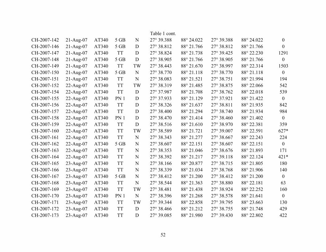
Table 1. Surface and midwater stations sampled over three cold seep sites (AT340, GC852, and AC601) (see Fig.1) in the Gulf of Mexico (9-25 August 2007). TT = Tucker trawl including plankton net inside Tucker trawl, PN 1 = 0.5 m dia. plankton net, PN 2 = 1 m dia. plankton net, NN = Neuston net, 5 GB = 5 gallon bucket for POM samples, D = day (0730 to 1830 hr CDT), N = night (2030 to 0530 hr CDT), TW = twilight (0530 to 0730 and 1830 to 2030 hr CDT). * = maximum depths sampled for non discrete tows (TT did not close and fished to surface). Blanks in depth columns indicated TDR did not record any data.

Station Date Site Gear Time Start Latitude

Start Longitude

End Latitude

End Longitude

Mean Depth Sampled (m)

CH-2007-002 09-Aug-07 GC852 TT N 27° 07.200 91° 09.769 27° 06.278 91° 09.945 611 CH-2007-003 09-Aug-07 GC852 TT N 27° 07.263 91° 09.781 27° 06.404 91° 10.023 390 CH-2007-004 10-Aug-07 GC852 5 GB N 27° 07.979 91° 09.028 27° 07.979 91° 09.028 0 CH-2007-005 10-Aug-07 GC852 TT N 27° 07.547 91° 09.694 27° 06.552 91° 09.927 323 CH-2007-006 10-Aug-07 GC852 5 GB N 27° 07.288 91° 09.771 27° 07.288 91° 09.771 0 CH-2007-007 10-Aug-07 GC852 TT N 27° 07.318 91° 09.736 27° 08.244 91° 09.480 296* CH-2007-008 10-Aug-07 GC852 TT N 27° 06.984 91° 09.844 27° 06.034 91° 10.025 303 CH-2007-009 10-Aug-07 GC852 PN 1 N 27° 07.042 91° 09.829 27° 06.048 91° 10.025 0 CH-2007-017 10-Aug-07 GC852 TT N 27° 07.407 91° 09.878 27° 06.436 91° 09.948 612 CH-2007-018 10-Aug-07 GC852 TT N 27° 06.354 91° 09.929 27° 07.386 91° 09.858 486* CH-2007-019 10-Aug-07 GC852 TT N 27° 07.823 91° 09.780 27° 06.975 91° 09.917 410 CH-2007-020 11-Aug-07 GC852 TT N 27° 05.979 91° 09.940 27° 07.053 91° 09.864 197 CH-2007-021 11-Aug-07 GC852 TT N 27° 07.074 91° 09.893 27° 06.278 91° 09.982 249 CH-2007-022 11-Aug-07 GC852 TT N 27° 06.550 91° 09.957 27° 07.604 91° 09.886 345 CH-2007-023 11-Aug-07 GC852 TT N 27° 07.715 91° 09.851 27° 06.680 91° 09.963 712* CH-2007-024 11-Aug-07 GC852 PN 1 N 27° 08.093 91° 09.807 27° 07.078 91° 09.925 0 CH-2007-028 11-Aug-07 GC852 PN 1 D 27° 07.769 91° 09.810 27° 08.269 91° 09.817 0 CH-2007-029 11-Aug-07 GC852 TT D 27° 10.481 91° 09.684 27° 09.381 91° 09.547 722 CH-2007-030 11-Aug-07 GC852 TT TW 27° 07.591 91° 09.272 27° 06.815 91° 09.939 378 CH-2007-031 11-Aug-07 GC852 TT N 27° 06.280 91° 10.229 27° 07.036 91° 09.676 382* CH-2007-032 11-Aug-07 GC852 TT N 27° 07.289 91° 09.857 27° 06.706 91° 10.685 492 CH-2007-033 12-Aug-07 GC852 TT N 27° 06.204 91° 10.505 27° 07.071 91° 09.742 248

48

Table 1 cont. CH-2007-034 12-Aug-07 GC852 5 GB N 27° 06.928 91° 09.881 27° 06.928 91° 09.881 0 CH-2007-035 12-Aug-07 GC852 TT N 27° 07.282 91° 09.630 27° 06.444 91° 10.342 155 CH-2007-036 12-Aug-07 GC852 TT N 27° 06.467 91° 10.403 27° 07.270 91° 09.604 149 CH-2007-037 12-Aug-07 GC852 TT N 27° 07.284 91° 09.637 27° 06.455 91° 10.320 185 CH-2007-038 12-Aug-07 GC852 TT N 27° 06.779 91° 10.077 27° 08.391 91° 08.713 462 CH-2007-039 12-Aug-07 GC852 PN 1 N 27° 08.036 91° 08.901 27° 08.138 91° 08.817 0 CH-2007-041 12-Aug-07 GC852 PN 1 D 27° 02.139 91° 09.618 27° 01.057 91° 09.738 0 CH-2007-043 12-Aug-07 GC852 NN D 27° 10.116 91° 09.910 27° 10.824 91° 09.867 0 CH-2007-044 12-Aug-07 GC852 TT D 27° 12.181 91° 09.454 27° 10.146 91° 09.474 791 CH-2007-045 12-Aug-07 GC852 TT TW 27° 08.756 91° 09.574 27° 07.816 91° 09.565 551 CH-2007-046 12-Aug-07 GC852 TT N 27° 06.034 91° 09.704 27° 05.290 91° 09.704 325* CH-2007-047 12-Aug-07 GC852 TT N 27° 05.665 91° 09.647 27° 06.713 91° 09.744 273 CH-2007-048 12-Aug-07 GC852 TT N 27° 07.203 91° 09.795 27° 06.338 91° 09.781 195 CH-2007-049 13-Aug-07 GC852 TT N 27° 06.454 91° 09.621 27° 07.493 91° 09.626 455 CH-2007-050 13-Aug-07 GC852 TT N 27° 07.626 91° 09.789 27° 06.726 91° 09.752 671 CH-2007-051 13-Aug-07 GC852 5 GB N 27° 07.516 91° 09.790 27° 07.516 91° 09.790 0 CH-2007-052 13-Aug-07 GC852 PN 1 N 27° 07.274 91° 09.786 27° 06.794 91° 09.760 0 CH-2007-053 13-Aug-07 GC852 TT N 27° 06.415 91° 09.700 27° 05.454 91° 09.695 484 CH-2007-054 13-Aug-07 GC852 TT TW 27° 08.270 91° 09.827 27° 07.304 91° 09.805 239 CH-2007-063 13-Aug-07 GC852 TT TW 27° 07.349 91° 10.193 27° 06.229 91° 10.163 406 CH-2007-064 13-Aug-07 GC852 TT N 27° 05.002 91° 10.098 27° 06.993 91° 10.152 195 CH-2007-065 13-Aug-07 GC852 TT N 27° 07.318 91° 10.205 27° 06.339 91° 10.338 154 CH-2007-066 13-Aug-07 GC852 TT N 27° 06.364 91° 10.472 27° 07.361 91° 10.404 642 CH-2007-067 13-Aug-07 GC852 5 GB N 27° 07.166 91° 10.418 27° 07.166 91° 10.418 0 CH-2007-068 14-Aug-07 GC852 TT N 27° 07.655 91° 10.406 27° 06.498 91° 10.396 657 CH-2007-069 14-Aug-07 GC852 PN 1 N 27° 07.505 91° 10.418 27° 07.015 91° 10.406 0 CH-2007-070 14-Aug-07 GC852 TT N 27° 06.208 91° 10.393 27° 07.194 91° 10.422 498 CH-2007-071 14-Aug-07 GC852 TT N 27° 07.462 91° 10.356 27° 06.522 91° 10.354 208

49

Table 1 cont. CH-2007-072 14-Aug-07 GC852 TT N 27° 06.686 91° 10.480 27° 07.828 91° 10.481 368 CH-2007-075 14-Aug-07 GC852 NN D 27° 08.616 91° 10.180 27° 08.149 91° 10.169 0 CH-2007-076 14-Aug-07 GC852 5 GB D 27° 06.656 91° 10.079 27° 06.656 91° 10.079 0 CH-2007-078 14-Aug-07 GC852 NN D 27° 09.228 91° 11.366 27° 08.309 91° 09.667 0 CH-2007-079 14-Aug-07 GC852 5 GB D 27° 09.388 91° 09.765 27° 09.388 91° 09.765 0 CH-2007-080 14-Aug-07 GC852 TT D 27° 10.379 91° 09.659 27° 09.372 91° 09.736 899 CH-2007-081 14-Aug-07 GC852 5 GB D 27° 09.660 91° 09.695 27° 09.660 91° 09.695 0 CH-2007-082 14-Aug-07 GC852 TT D 27° 07.841 91° 09.948 27° 06.897 91° 09.925 201 CH-2007-083 14-Aug-07 GC852 TT TW 27° 05.076 91° 09.857 27° 04.136 91° 09.852 763 CH-2007-084 14-Aug-07 GC852 TT N 27° 05.194 91° 09.691 27° 06.258 91° 09.810 480 CH-2007-085 14-Aug-07 GC852 TT N 27° 07.000 91° 09.830 27° 06.055 91° 09.802 350 CH-2007-086 14-Aug-07 GC852 TT N 27° 06.133 91° 09.832 27° 07.162 91° 09.915 791 CH-2007-087 15-Aug-07 GC852 TT N 27° 07.043 91° 09.791 27° 06.157 91° 09.875 966 CH-2007-088 15-Aug-07 GC852 TT N 27° 05.024 91° 09.692 27° 06.632 91° 09.703 518 CH-2007-089 15-Aug-07 GC852 TT N 27° 07.452 91° 09.710 27° 06.456 91° 09.731 150 CH-2007-090 15-Aug-07 GC852 TT TW 27° 06.872 91° 10.013 27° 07.949 91° 10.191 423 CH-2007-092 15-Aug-07 GC852 TT D 27° 08.468 91° 07.273 27° 07.702 91° 06.813 1004 CH-2007-093 15-Aug-07 GC852 TT D 27° 09.883 91° 09.198 27° 09.065 91° 08.610 1035 CH-2007-094 15-Aug-07 GC852 TT D 27° 09.020 91° 09.419 27° 08.421 91° 08.831 CH-2007-095 15-Aug-07 GC852 TT D 27° 08.001 91° 09.940 27° 07.224 91° 09.176 586 CH-2007-096 15-Aug-07 GC852 TT D 27° 06.985 91° 10.006 27° 07.324 91° 09.216 569* CH-2007-097 15-Aug-07 GC852 TT TW 27° 06.474 91° 10.045 27° 06.090 91° 09.078 332 CH-2007-098 15-Aug-07 GC852 TT N 27° 05.122 91° 10.161 27° 04.635 91° 09.361 723 CH-2007-099 15-Aug-07 GC852 TT N 27° 06.869 91° 09.295 27° 04.437 91° 08.386 606 CH-2007-101 16-Aug-07 GC852 TT TW 27° 06.882 91° 09.207 27° 06.447 91° 08.140 493 CH-2007-103 16-Aug-07 GC852 TT D 27° 07.981 91° 10.268 27° 07.663 91° 09.187 555 CH-2007-104 16-Aug-07 GC852 TT D 27° 06.933 91° 10.182 27° 06.401 91° 09.166 CH-2007-105 16-Aug-07 GC852 TT D 27° 06.146 91° 10.299 27° 05.025 91° 10.148 915

50

Table 1 cont. CH-2007-106 16-Aug-07 GC852 TT D 27° 05.257 91° 10.480 27° 06.145 91° 10.673 1067 CH-2007-107 16-Aug-07 GC852 TT TW 27° 07.714 91° 10.575 27° 06.697 91° 10.493 287 CH-2007-108 16-Aug-07 GC852 TT TW 27° 05.657 91° 09.916 27° 04.715 91° 09.464 139 CH-2007-110 16-Aug-07 GC852 TT N 27° 05.265 91° 09.515 27° 06.212 91° 09.680 473 CH-2007-111 16-Aug-07 GC852 TT N 27° 07.135 91° 09.955 27° 06.190 91° 10.241 94 CH-2007-112 16-Aug-07 GC852 TT N 27° 06.082 91° 10.482 27° 06.929 91° 10.661 138 CH-2007-113 17-Aug-07 GC852 TT N 27° 06.958 91° 10.845 27° 06.001 91° 10.946 59 CH-2007-114 17-Aug-07 GC852 TT N 27° 05.795 91° 10.799 27° 06.978 91° 10.690 51 CH-2007-115 17-Aug-07 GC852 TT N 27° 07.113 91° 10.611 27° 06.010 91° 10.542 81 CH-2007-116 17-Aug-07 GC852 TT N 27° 05.701 91° 10.320 27° 07.004 91° 10.227 21 CH-2007-117 17-Aug-07 GC852 TT N 27° 06.340 91° 10.268 27° 05.345 91° 10.336 540 CH-2007-118 17-Aug-07 AC601 TT N 26° 23.314 94° 30.559 26° 22.580 94° 31.020 253 CH-2007-119 18-Aug-07 AC601 TT N 26° 23.215 94° 30.841 26° 24.247 94° 30.814 171 CH-2007-120 18-Aug-07 AC601 PN 1 N 26° 22.991 94° 30.838 26° 23.584 94° 30.851 0 CH-2007-121 18-Aug-07 AC601 5 GB N 26° 24.247 94° 30.814 26° 24.247 94° 30.814 0 CH-2007-122 18-Aug-07 AC601 TT N 26° 23.450 94° 30.771 26° 22.905 94° 30.832 584 CH-2007-123 18-Aug-07 AC601 5 GB N 26° 22.941 94° 30.823 26° 22.941 94° 30.823 0 CH-2007-124 18-Aug-07 AC601 TT N 26° 22.962 94° 30.903 26° 24.152 94° 31.038 318 CH-2007-125 18-Aug-07 AC601 5 GB N 26° 23.705 94° 30.996 26° 23.705 94° 30.996 0 CH-2007-126 18-Aug-07 AC601 TT N 26° 24.786 94° 31.143 26° 23.872 94° 31.135 45 CH-2007-129 18-Aug-07 AC601 5 GB D 26° 23.683 94° 30.923 26° 23.683 94° 30.923 0 CH-2007-133 18-Aug-07 AC601 5 GB D 26° 22.504 94° 31.365 26° 22.504 94° 31.365 0 CH-2007-136 20-Aug-07 AT340 TT TW 27° 38.175 88° 21.014 27° 38.083 88° 21.956 331 CH-2007-137 20-Aug-07 AT340 TT N 27° 38.258 88° 21.699 27° 38.066 88° 22.702 264 CH-2007-138 20-Aug-07 AT340 TT N 27° 38.876 88° 21.910 27° 38.752 88° 22.889 217 CH-2007-139 21-Aug-07 AT340 TT N 27° 38.685 88° 22.052 27° 38.593 88° 23.286 124 CH-2007-140 21-Aug-07 AT340 TT N 27° 38.659 88° 22.195 27° 38.642 88° 23.122 425 CH-2007-141 21-Aug-07 AT340 TT N 27° 38.733 88° 22.647 27° 38.862 88° 23.578 586

51

Table 1 cont. CH-2007-142 21-Aug-07 AT340 5 GB N 27° 39.388 88° 24.022 27° 39.388 88° 24.022 0 CH-2007-146 21-Aug-07 AT340 5 GB D 27° 38.812 88° 21.766 27° 38.812 88° 21.766 0 CH-2007-147 21-Aug-07 AT340 TT D 27° 38.824 88° 21.738 27° 39.425 88° 22.230 1291 CH-2007-148 21-Aug-07 AT340 5 GB D 27° 38.905 88° 21.766 27° 38.905 88° 21.766 0 CH-2007-149 21-Aug-07 AT340 TT TW 27° 38.443 88° 21.670 27° 38.997 88° 22.314 1503 CH-2007-150 21-Aug-07 AT340 5 GB N 27° 38.770 88° 21.118 27° 38.770 88° 21.118 0 CH-2007-151 21-Aug-07 AT340 TT N 27° 38.083 88° 21.521 27° 38.751 88° 21.994 194 CH-2007-152 22-Aug-07 AT340 TT TW 27° 38.319 88° 21.485 27° 38.875 88° 22.066 542 CH-2007-154 22-Aug-07 AT340 TT D 27° 37.987 88° 21.708 27° 38.762 88° 22.018 539 CH-2007-155 22-Aug-07 AT340 PN 1 D 27° 37.933 88° 21.129 27° 37.921 88° 21.422 0 CH-2007-156 22-Aug-07 AT340 TT D 27° 38.326 88° 21.637 27° 38.811 88° 21.935 842 CH-2007-157 22-Aug-07 AT340 TT D 27° 38.400 88° 21.294 27° 38.740 88° 21.934 984 CH-2007-158 22-Aug-07 AT340 PN 1 D 27° 38.470 88° 21.414 27° 38.460 88° 21.402 0 CH-2007-159 22-Aug-07 AT340 TT D 27° 38.516 88° 21.610 27° 38.970 88° 22.381 359 CH-2007-160 22-Aug-07 AT340 TT TW 27° 38.589 88° 21.721 27° 39.007 88° 22.591 627* CH-2007-161 22-Aug-07 AT340 TT N 27° 38.343 88° 21.277 27° 38.667 88° 22.243 224 CH-2007-162 22-Aug-07 AT340 5 GB N 27° 38.607 88° 22.151 27° 38.607 88° 22.151 0 CH-2007-163 22-Aug-07 AT340 TT N 27° 38.353 88° 21.046 27° 38.676 88° 21.893 171 CH-2007-164 22-Aug-07 AT340 TT N 27° 38.392 88° 21.217 27° 39.118 88° 22.124 421* CH-2007-165 23-Aug-07 AT340 TT N 27° 38.166 88° 20.877 27° 38.715 88° 21.805 180 CH-2007-166 23-Aug-07 AT340 TT N 27° 38.339 88° 21.034 27° 38.768 88° 21.906 140 CH-2007-167 23-Aug-07 AT340 5 GB N 27° 38.412 88° 21.200 27° 38.412 88° 21.200 0 CH-2007-168 23-Aug-07 AT340 TT N 27° 38.544 88° 21.363 27° 38.880 88° 22.181 63 CH-2007-169 23-Aug-07 AT340 TT TW 27° 38.481 88° 21.438 27° 38.924 88° 22.252 160 CH-2007-170 23-Aug-07 AT340 PN 1 N 27° 38.396 88° 21.268 27° 38.578 88° 21.641 0 CH-2007-171 23-Aug-07 AT340 TT TW 27° 39.344 88° 22.858 27° 39.795 88° 23.663 130 CH-2007-172 23-Aug-07 AT340 TT D 27° 38.466 88° 21.212 27° 38.755 88° 21.748 429 CH-2007-173 23-Aug-07 AT340 TT D 27° 39.085 88° 21.980 27° 39.430 88° 22.802 422

52

Table 1 cont. CH-2007-174 23-Aug-07 AT340 5 GB D 27° 39.034 88° 21.969 27° 39.034 88° 21.969 0 CH-2007-175 23-Aug-07 AT340 TT D 27° 38.006 88° 20.645 27° 38.178 88° 21.475 511 CH-2007-176 23-Aug-07 AT340 TT D 27° 38.657 88° 21.842 27° 38.890 88° 22.623 253 CH-2007-177 23-Aug-07 AT340 PN 1 D 27° 38.640 88° 21.781 27° 38.872 88° 22.582 0 CH-2007-178 23-Aug-07 AT340 TT D 27° 38.400 88° 21.216 27° 38.765 88° 22.082 321 CH-2007-179 23-Aug-07 AT340 5 GB D 27° 38.383 88° 21.177 27° 38.383 88° 21.177 0 CH-2007-180 23-Aug-07 AT340 TT D 27° 39.436 88° 23.669 27° 39.813 88° 24.614 484 CH-2007-181 23-Aug-07 AT340 PN 2 D 27° 39.326 88° 23.419 27° 39.653 88° 24.196 0 CH-2007-182 23-Aug-07 AT340 TT D 27° 38.522 88° 21.466 27° 38.879 88° 22.379 669 CH-2007-183 23-Aug-07 AT340 TT TW 27° 38.343 88° 21.041 27° 38.728 88° 21.036 134 CH-2007-184 23-Aug-07 AT340 TT N 27° 38.169 88° 20.947 27° 38.559 88° 21.804 633 CH-2007-185 23-Aug-07 AT340 PN 2 N 27° 38.183 88° 20.712 27° 38.226 88° 20.129 0 CH-2007-186 23-Aug-07 AT340 TT N 27° 38.280 88° 21.203 27° 38.819 88° 22.169 382 CH-2007-187 23-Aug-07 AT340 PN 2 N 27° 38.235 88° 20.784 27° 38.434 88° 21.485 0 CH-2007-188 24-Aug-07 AT340 TT N 27° 38.566 88° 21.511 27° 38.941 88° 22.385 285 CH-2007-189 24-Aug-07 AT340 TT N 27° 38.460 88° 21.314 27° 38.848 88° 22.197 278 CH-2007-190 24-Aug-07 AT340 5 GB N 27° 38.291 88° 20.933 27° 38.291 88° 20.933 0 CH-2007-191 24-Aug-07 AT340 TT N 27° 38.463 88° 21.357 27° 38.837 88° 22.285 267 CH-2007-192 24-Aug-07 AT340 TT N 27° 38.832 88° 22.322 27° 39.206 88° 23.222 261 CH-2007-198 24-Aug-07 AT340 TT TW 27° 38.767 88° 21.397 27° 39.120 88° 22.339 292 CH-2007-199 24-Aug-07 AT340 TT N 27° 38.718 88° 21.795 27° 39.237 88° 22.684 114 CH-2007-200 24-Aug-07 AT340 TT N 27° 38.611 88° 21.584 27° 39.101 88° 22.504 540 CH-2007-201 24-Aug-07 AT340 PN 2 N 27° 38.335 88° 21.133 27° 38.665 88° 21.757 0 CH-2007-202 24-Aug-07 AT340 TT N 27° 38.640 88° 21.675 27° 39.095 88° 22.586 410 CH-2007-203 24-Aug-07 AT340 PN 2 N 27° 38.387 88° 21.184 27° 38.757 88° 21.929 0 CH-2007-204 24-Aug-07 AT340 TT N 27° 38.644 88° 21.662 27° 39.110 88° 22.691 572 CH-2007-205 24-Aug-07 AT340 TT N 27° 38.706 88° 21.715 27° 39.100 88° 22.662 395 CH-2007-206 24-Aug-07 AT340 PN 2 N 27° 38.415 88° 21.190 27° 38.819 88° 21.964 0

53

Table 1 cont. CH-2007-210 25-Aug-07 AT340 TT D 27° 38.651 88° 21.414 27° 38.828 88° 22.558 142* CH-2007-211 25-Aug-07 AT340 TT D 27° 39.026 88° 24.074 27° 39.195 88° 25.116 868 CH-2007-213 25-Aug-07 AT340 TT TW 27° 38.782 88° 21.433 27° 38.881 88° 22.279 354 CH-2007-214 25-Aug-07 AT340 TT TW 27° 38.600 88° 21.459 27° 38.857 88° 22.587 307 CH-2007-215 25-Aug-07 AT340 PN 2 N 27° 38.479 88° 21.082 27° 38.785 88° 22.031 0 CH-2007-216 25-Aug-07 AT340 TT N 27° 38.573 88° 21.399 27° 38.848 88° 22.497 528 CH-2007-217 25-Aug-07 AT340 PN 2 N 27° 38.577 88° 21.421 27° 38.838 88° 22.485 0 CH-2007-218 25-Aug-07 AT340 TT N 27° 38.649 88° 21.746 27° 38.834 88° 22.774 579 CH-2007-219 25-Aug-07 AT340 TT N 27° 38.777 88° 21.981 27° 39.923 88° 23.041 78 CH-2007-220 25-Aug-07 AT340 TT N 27° 38.802 88° 22.198 27° 38.998 88° 23.552 1149 CH-2007-221 25-Aug-07 AT340 PN 2 N 27° 38.565 88° 20.778 27° 38.698 88° 21.596 0

54

Table 2. The total number of all midwater fishes, invertebrates and autotrophs examined in dietary analyses from the North-central GOM. GCA = gut content analysis. SIA = stable isotope analysis, SL range = standard length size range for fish species (mm). Fish species marked with an * were grouped at family level for all analyses. Fish species marked with ^ were grouped at genera for stable isotope analyses. Species GCA SIA SL range FISH

Gonostomatidae Cyclothone acclinidens 1 46 Cyclothone alba 290 5 10-33 Cyclothone braueri 319 11-28 Cyclothone pallida 362 10 12-51 Cyclothone pseudopallida 332 10 12-45 Gonostoma elongatum 88 12 21-190

Sternoptychidae Argyropelecus aculeatus 40 10 13-56 Argyropelecus hemigymnus 30 10 8-30 Sternoptyx diaphana^ 5 22-28 Sternoptyx pseudobscura^ 4 32-49 Valenciennellus tripunctulatus 147 15 13-30

Phosichthyidae Pollichthys mauli 63 10 14-51 Vinciguerria poweriae 155 15 12-35

Stomiidae Astronesthes macropogon* 2 21, 34 Astronesthes similus* 3 20-31 Bathophilus longipinnis* 2 41-65 Bathophilus pawneei* 1 31 Chauliodus sloani 63 6 20-132 Eustomias lipochirus* 1 1 80 Eustomias schmidti* 1 1 80 Leptostomias bilobatus* 1 1 105 Melanostomias biseriatus* 1 40 Melanostomias valdiviae* 1 31 Photonectes margarita* 1 260 Photostomias guernei* 8 5 49-117 Stomias affinis* 14 2 23-90 Stomias longibarbatus* 1 86

Myctophidae Benthosema suborbitale 234 6 10-30 Ceratoscopelus warmingii 88 12 15-45

55

Table 2 cont. Diaphus lucidus^ 2 27, 67 Diaphus mollis^ 34 4 12-55 Diaphus problematicus 7 45-74 Hygophum benoiti 111 12-22 Lampanyctus alatus 72 15 14-52 Lepidophanes guentheri 157 10 14-66 Myctophum affine 61 10 13-18 Notolychnus valdiviae 343 11-22

Melamphaidae Melamphaes simus* 7 14-26 Melamphaes typhlops* 2 22, 25 Scopelogadus mizolepis* 1 24

AMPHIPODA Phrosinidae

Anchylomera blossevillei 1 Platyscelidae 1

Platyscelus sp. 2 Pronoidae

Parapronoe sp. 1 CEPHALOPODA

Bolitaenidae Japetella diaphana 1

Enoploteuthidae Ancistrocheirus lesuerii 1

Histioteuthidae Stigmatoteuthis arcturi 3

CHAETOGNATHA 5 CNIDARIA

Rhopalonematidae Colobonema sericeum 1

Atollidae 1 Atolla vanhoeffeni 1

COPEPODA 6 Megacalanidae

Bathycalanus princeps 4 Pontellidae

Labidocera sp. 2 DECAPODA

Benthesicymidae Gennadas valens 14

56

57

Table 2 cont. Oplophoridae

Acanthephyra purpurea 5 Systellaspis debilis 7

Sergestidae Sergia sp. 1

EUPHAUSIACEA 11 Euphausiidae

Nematoscelis megalops 3 Thysanopoda sp. 2 Thysanopoda tricuspida 2

GASTROPODA Cavoliniidae

Cavolinia tridentata 1 Diacavolinia sp. 2

SALPIDA Salpidae

Salpa cylindrica 4 Salpa sp. 6

ZOOPLANKTON 11 AUTOTROPH

Sargassaceae Sargassum fluitans 2 Sargassum sp. 10

Phytoplankton 21 Detritus 5

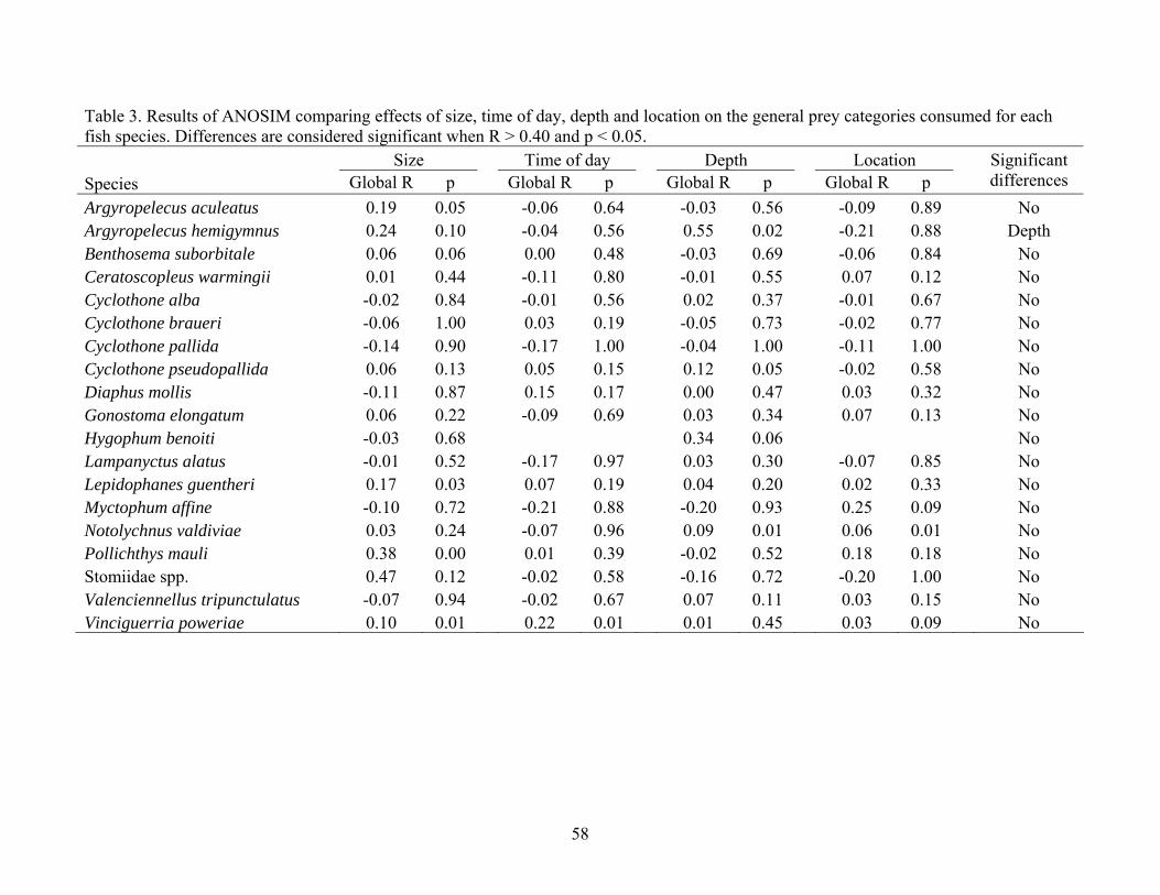
Table 3. Results of ANOSIM comparing effects of size, time of day, depth and location on the general prey categories consumed for each fish species. Differences are considered significant when R > 0.40 and p < 0.05. Size Time of day Depth Location Species Global R p Global R p Global R p Global R p

Significant differences

Argyropelecus aculeatus 0.19 0.05 -0.06 0.64 -0.03 0.56 -0.09 0.89 No Argyropelecus hemigymnus 0.24 0.10 -0.04 0.56 0.55 0.02 -0.21 0.88 Depth Benthosema suborbitale 0.06 0.06 0.00 0.48 -0.03 0.69 -0.06 0.84 No Ceratoscopleus warmingii 0.01 0.44 -0.11 0.80 -0.01 0.55 0.07 0.12 No Cyclothone alba -0.02 0.84 -0.01 0.56 0.02 0.37 -0.01 0.67 No Cyclothone braueri -0.06 1.00 0.03 0.19 -0.05 0.73 -0.02 0.77 No Cyclothone pallida -0.14 0.90 -0.17 1.00 -0.04 1.00 -0.11 1.00 No Cyclothone pseudopallida 0.06 0.13 0.05 0.15 0.12 0.05 -0.02 0.58 No Diaphus mollis -0.11 0.87 0.15 0.17 0.00 0.47 0.03 0.32 No Gonostoma elongatum 0.06 0.22 -0.09 0.69 0.03 0.34 0.07 0.13 No Hygophum benoiti -0.03 0.68 0.34 0.06 No Lampanyctus alatus -0.01 0.52 -0.17 0.97 0.03 0.30 -0.07 0.85 No Lepidophanes guentheri 0.17 0.03 0.07 0.19 0.04 0.20 0.02 0.33 No Myctophum affine -0.10 0.72 -0.21 0.88 -0.20 0.93 0.25 0.09 No Notolychnus valdiviae 0.03 0.24 -0.07 0.96 0.09 0.01 0.06 0.01 No Pollichthys mauli 0.38 0.00 0.01 0.39 -0.02 0.52 0.18 0.18 No Stomiidae spp. 0.47 0.12 -0.02 0.58 -0.16 0.72 -0.20 1.00 No Valenciennellus tripunctulatus -0.07 0.94 -0.02 0.67 0.07 0.11 0.03 0.15 No Vinciguerria poweriae 0.10 0.01 0.22 0.01 0.01 0.45 0.03 0.09 No

58

Table 4. Percent volume and frequency of prey items consumed by Chauliodus sloani collected from three sites in the Gulf of Mexico (AC601, GC852, AT340) separated by time of day. Night = 2030 to 0530 hr CDT, Day = 0730 to 1830 hr CDT, Twilight = 0530 to 0730 and 1830 to 2030; n = total number of stomachs analyzed; E = number of stomachs empty. AC601 GC852 AT340 Night Day Night Twilight Day Night Twilight n = 2 n = 8 n = 37 n = 2 n = 5 n = 7 n = 2 E = 2 E = 7 E = 30 E = 1 E = 5 E = 6 E = 1 Food Item %V %F %V %F %V %F %V %F %V %F %V %F %V %F FISH 100.0 100.0 86.5 28.6 100.0 100.0 100.0 100.0 Bregmaceros spp. 100.0 100.0 Myctophidae 67.5 14.3 Unidentified fish parts 19.0 14.3 100.0 100.0 100.0 100.0 CRUSTACEA <0.1 14.3 Unidentified crustacean parts <0.1 14.3 OTHER 13.5 71.4 100.0 100.0 Organic material 13.0 57.1 100.0 100.0 Unidentified animal parts 0.5 14.3

59

Table 5. Percent volume and frequency of prey items consumed by Gonostoma elongatum collected from three sites in the Gulf of Mexico (AC601, GC852, AT340) separated by time of day. Night = 2030 to 0530 hr CDT, Day = 0730 to 1830 hr CDT, Twilight = 0530 to 0730 and 1830 to 2030; n = total number of stomachs analyzed; E = number of stomachs empty. AC601 GC852 AT340 Night Day Night Twilight Day Night Twilight n = 0 n = 2 n = 28 n = 3 n = 3 n = 42 n = 10 E = 0 E = 0 E = 11 E = 0 E = 0 E = 10 E = 0 Food Item %V %F %V %F %V %F %V %F %V %F %V %F %V %F AMPHIPODA 0.7 11.8 0.3 3.1 Amphipoda 0.7 11.8 Scina pusilla 0.3 3.1 CHAETOGNATHA 3.4 5.9 Heterokrohnia sp. 3.4 5.9 CNIDARIA 0.4 5.9 Cnidaria 0.4 5.9 18.0 20.0 COPEPODA 2.2 35.3 0.4 33.3 1.6 34.4 Aetideus acutus <0.1 5.9 Calanoida 0.5 17.6 0.1 3.1 Candacia longimana 14.4 10.0 Copepoda 0.1 11.8 0.3 9.4 3.6 10.0 Corycaeus furcifer <0.1 33.3 Corycaeus sp. 0.1 5.9 <0.1 3.1 Eucalanidae <0.1 3.1 Gaetanus pileatus 0.4 3.1 Haloptilus sp. 0.6 5.9 Pareucalanus attenuatus 0.1 3.1 Pleuromamma xiphias 0.7 11.8 0.4 3.1 Rhincalanus cornutus 0.4 33.3 Temora stylifera <0.1 5.9

60

Table 5 cont. Unidentified copepod parts 0.2 11.8 0.3 12.5 CRUSTACEA 7.3 41.2 14.0 100.0 41.3 33.3 3.4 46.9 25.3 40.0 Unidentified crustacean parts 7.3 41.2 14.0 100.0 41.3 33.3 3.4 46.9 25.3 40.0 DECAPODA 0.6 33.3 86.9 6.3 Decapoda 0.6 33.3 86.9 6.3 EUPHAUSIACEA 17.8 11.8 61.6 33.3 3.8 9.4 Euphausiidae 17.8 11.8 14.7 33.3 2.1 9.4 Thysanoessa sp. 1.7 3.1 Thysanopoda sp. 46.9 33.3 MYSIDICEA 2.1 5.9 Lophogastridae 2.1 5.9 OSTRACODA 0.1 17.6 0.1 6.3 Halocyprididae 0.1 11.8 <0.1 3.1 Myodocopida 0.1 3.1 Ostracoda <0.1 5.9 OTHER 100.0 100.0 66.0 64.7 23.4 100.0 58.7 100.0 4.0 62.5 56.7 90.0 Organic material 100.0 100.0 63.7 52.9 23.4 100.0 58.7 100.0 3.4 62.5 56.7 90.0 Unidentified animal parts 2.3 11.8 0.6 3.1

61

Table 6. Percent volume and frequency of prey items consumed by Stomiidae collected from three sites in the Gulf of Mexico (AC601, GC852, AT340) separated by time of day. Night = 2030 to 0530 hr CDT, Day = 0730 to 1830 hr CDT, Twilight = 0530 to 0730 and 1830 to 2030; n = total number of stomachs analyzed; E = number of stomachs empty. AC601 GC852 AT340 Night Day Night Twilight Day Night Twilight n = 1 n = 5 n = 13 n = 3 n = 0 n = 8 n = 6 E = 1 E = 2 E = 9 E = 2 E = 0 E = 6 E = 5 Food Item %V %F %V %F %V %F %V %F %V %F %V %F %V %F COPEPODA 0.1 33.3 Oncaea sp. 0 33.3 Unidentified copepod parts 0.1 33.3 DECAPODA 61.4 33.3 8.3 25.0 Decapoda 8.3 25.0 Penaeidae 61.4 33.3 FISH 7.5 66.7 27.5 25.0 100.0 100.0 80.7 50.0 100.0 100.0 Diaphus mollis 100.0 100.0 Myctophidae 44.2 50.0 Unidentified fish parts 7.5 66.7 27.5 25.0 36.4 50.0 100.0 100.0OTHER 31.1 66.7 19.3 100.0 Invertebrate <0.1 33.3 Nematoda 3.3 33.3 64.2 50.0 Organic material 27.7 33.3 58.7 50.0 19.3 100.0 Unidentified animal parts 5.5 50.0

62

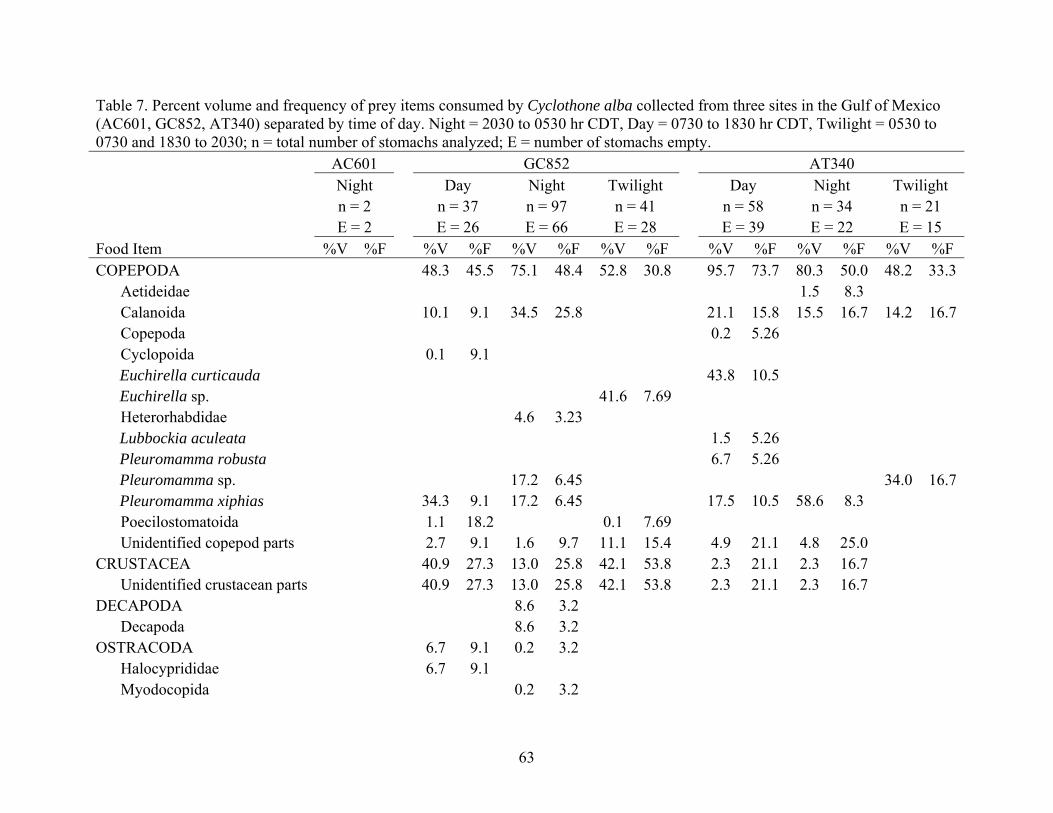
Table 7. Percent volume and frequency of prey items consumed by Cyclothone alba collected from three sites in the Gulf of Mexico (AC601, GC852, AT340) separated by time of day. Night = 2030 to 0530 hr CDT, Day = 0730 to 1830 hr CDT, Twilight = 0530 to 0730 and 1830 to 2030; n = total number of stomachs analyzed; E = number of stomachs empty. AC601 GC852 AT340 Night Day Night Twilight Day Night Twilight n = 2 n = 37 n = 97 n = 41 n = 58 n = 34 n = 21 E = 2 E = 26 E = 66 E = 28 E = 39 E = 22 E = 15 Food Item %V %F %V %F %V %F %V %F %V %F %V %F %V %F COPEPODA 48.3 45.5 75.1 48.4 52.8 30.8 95.7 73.7 80.3 50.0 48.2 33.3

Aetideidae 1.5 8.3 Calanoida 10.1 9.1 34.5 25.8 21.1 15.8 15.5 16.7 14.2 16.7 Copepoda 0.2 5.26 Cyclopoida 0.1 9.1

Euchirella curticauda 43.8 10.5 Euchirella sp. 41.6 7.69

Heterorhabdidae 4.6 3.23 Lubbockia aculeata 1.5 5.26 Pleuromamma robusta 6.7 5.26 Pleuromamma sp. 17.2 6.45 34.0 16.7 Pleuromamma xiphias 34.3 9.1 17.2 6.45 17.5 10.5 58.6 8.3

Poecilostomatoida 1.1 18.2 0.1 7.69 Unidentified copepod parts 2.7 9.1 1.6 9.7 11.1 15.4 4.9 21.1 4.8 25.0

CRUSTACEA 40.9 27.3 13.0 25.8 42.1 53.8 2.3 21.1 2.3 16.7 Unidentified crustacean parts 40.9 27.3 13.0 25.8 42.1 53.8 2.3 21.1 2.3 16.7

DECAPODA 8.6 3.2 Decapoda 8.6 3.2

OSTRACODA 6.7 9.1 0.2 3.2 Halocyprididae 6.7 9.1 Myodocopida 0.2 3.2

63

Table 7 cont. OTHER 4.1 36.4 3.0 25.8 5.0 30.8 2.0 10.5 17.4 41.7 51.8 66.7

Organic material 4.0 27.3 3.0 22.6 5.0 30.8 2.0 10.5 6.5 33.3 49.6 66.7 Nematoda 0.1 9.1 0.1 6.5 1.7 25.0 2.3 33.3 Unidentified animal parts 9.1 8.3

64

Table 8. Percent volume and frequency of prey items consumed by Cyclothone braueri collected from three sites in the Gulf of Mexico (AC601, GC852, AT340) separated by time of day. Night = 2030 to 0530 hr CDT, Day = 0730 to 1830 hr CDT, Twilight = 0530 to 0730 and 1830 to 2030; n = total number of stomachs analyzed; E = number of stomachs empty. AC601 GC852 AT340 Night Day Night Twilight Day Night Twilight n = 2 n = 18 n = 100 n = 49 n = 55 n = 58 n = 37 E = 2 E = 14 E = 77 E = 34 E = 47 E = 41 E = 35 Food Item %V %F %V %F %V %F %V %F %V %F %V %F %V %F COPEPODA 100.0 100.0 64.3 39.1 53.0 66.7 42.4 87.5 69.2 52.9 7.0 50.0 Aegisthus mucronatus 57.2 25.0 19.7 13.3 16.2 25.0

Calanoida 10.9 8.7 2.6 6.7 5.3 25.0 36.6 17.6 7.0 50.0 Copepoda <0.1 4.35

Corycaeus sp. 3.6 25.0 Cyclopoida 0.2 4.35 0.4 5.88

Lubbockia aculeata 5.4 25.0 Miracia efferata 1.2 12.5 Pleuromamma sp. 35.0 8.7

Unidentified copepod parts 33.8 100.0 18.1 13 30.7 46.7 19.7 25.0 32.2 29.4 CRUSTACEA 23.0 43.5 27.6 58.8

Unidentified crustacean parts 23.0 43.5 27.6 58.8 OSTRACODA 1.2 4.35 35.2 20.0 57.6 25.0

Conchoecinae 54.2 12.5 Ostracoda 35.2 20.0 3.4 12.5 Unidentified ostracod parts 1.2 4.35

OTHER 11.5 39.1 11.8 20.0 3.2 29.4 93.0 50.0 Organic material 11.5 39.1 7.6 13.3 3.2 29.4 93.0 50.0 Unidentified animal parts 4.2 6.7

65

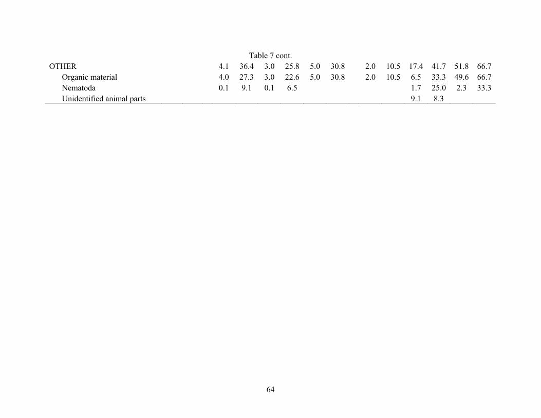
Table 9. Percent volume and frequency of prey items consumed by Cyclothone pseudopallida collected from three sites in the Gulf of Mexico (AC601, GC852, AT340) separated by time of day. Night = 2030 to 0530 hr CDT, Day = 0730 to 1830 hr CDT, Twilight = 0530 to 0730 and 1830 to 2030; n = total number of stomachs analyzed; E = number of stomachs empty. AC601 GC852 AT340 Night Day Night Twilight Day Night Twilight n = 12 n = 90 n = 95 n = 34 n = 46 n = 34 n = 21 E = 11 E = 71 E = 70 E = 25 E = 37 E = 22 E = 20 Food Item %V %F %V %F %V %F %V %F %V %F %V %F %V %F COPEPODA 100.0 100.0 87.5 52.6 47.8 48.0 39.5 55.6 86.3 77.8 92.1 75.0 100.0 100.0 Aegisthus mucronatus 0.6 4.0 9.1 11.1

Aetideidae 3.3 8.3 Calanoida 10.4 26.3 10.2 16.0 18.9 33.3 77.3 66.7 44.4 33.3 100.0 100.0

Chiridus sp. 11.2 11.1 Copepoda 34.4 5.3 0.6 4.0 Harpacticoida 0.3 8.3

Lubbockia aculeata 5.2 11.1 Lubbockia squillimana 4.1 11.1 Lubbockia sp. 0.3 5.3 Lucicutia sp. 0.0 4.0

Mormonilla phasma 22.3 5.3 Oithona sp. 0.3 5.3 Rhincalanus sp. 0.5 4.0 Pleuromamma xiphias 16.5 5.3 Pleuromamma sp. 18.7 4.0 Valdiviella minor 27.4 8.3

Unidentified copepod parts 100.0 100.0 3.3 10.5 35.9 16.0 16.7 8.3 CRUSTACEA 6.0 5.3 4.5 24.0 53.2 22.2 2.0 16.7

Unidentified crustacean parts 6.0 5.3 4.5 24.0 53.2 22.2 2.0 16.7

66

Table 9 cont. OSTRACODA 3.4 5.3 5.8 22.2 8.7 11.1 5.9 8.3

Conchoecinae 5.2 11.1 5.9 8.3 Halocyprididae Myodocopida 3.4 5.3 Ostracoda 0.6 11.1 8.7 11.1 Unidentified ostracod parts

OTHER 3.0 36.8 29.0 32 1.6 22.2 5.0 22.2 <0.1 8.3 Animalia 2.7 11.1 Nematoda <0.1 5.3 0.1 4.0 Organic material 3.0 31.6 28.9 28.0 1.3 11.1 2.3 11.1 <0.1 8.3 Unidentified animal parts 0.3 11.1

67

Table 10. Percent volume and frequency of prey items consumed by Hygophum benoiti collected from three sites in the Gulf of Mexico (AC601, GC852, AT340) separated by time of day. Night = 2030 to 0530 hr CDT, Day = 0730 to 1830 hr CDT, Twilight = 0530 to 0730 and 1830 to 2030; n = total number of stomachs analyzed; E = number of stomachs empty. AC601 GC852 AT340 Night Day Night Twilight Day Night Twilight n = 6 n = 23 n = 37 n = 10 n = 7 n = 27 n = 1 E = 6 E = 23 E = 37 E = 10 E = 6 E = 11 E = 1 Food Item %V %F %V %F %V %F %V %F %V %F %V %F %V %F AMPHIPODA 0.2 6.3

Amphipoda 0.2 6.3 COPEPODA 52.0 81.3

Calanoida 15.7 50.0 Candacia curta 1.4 6.3 Candacia pachydactyla 2.8 6.3

Cyclopoida 5.8 62.5 Farranula gracilis 0.9 25.0

Unidentified copepod parts 25.4 68.8 CRUSTACEA 100.0 100.0 9.2 25.0

Unidentified crustacean parts 100.0 100.0 9.2 25.0 DECAPODA 3.8 6.3

Decapoda 3.8 6.3 MOLLUSCA 0.2 18.8

Bivalvia 0.2 18.8 OSTRACODA 0.6 12.5

Myodocopida 0.1 6.3 Ostracoda 0.5 6.3

OTHER 34.0 75.0 Organic material 34.0 75.0

68

Table 11. Percent volume and frequency of prey items consumed by Valenciennellus tripunctulatus collected from three sites in the Gulf of Mexico (AC601, GC852, AT340) separated by time of day. Night = 2030 to 0530 hr CDT, Day = 0730 to 1830 hr CDT, Twilight = 0530 to 0730 and 1830 to 2030; n = total number of stomachs analyzed; E = number of stomachs empty. AC601 GC852 AT340 Night Day Night Twilight Day Night Twilight n = 1 n = 3 n = 37 n = 24 n = 9 n = 44 n = 29 E = 0 E = 0 E = 4 E = 3 E = 4 E = 12 E = 2 Food Item %V %F %V %F %V %F %V %F %V %F %V %F %V %F AMPHIPODA 0.3 9.5

Amphipoda <0.1 4.8 Unidentified amphipod parts 0.3 4.8

COPEPODA 1.2 100.0 28.8 33.3 24.8 51.5 58.4 85.7 84.8 80.0 40.0 62.5 59.2 77.8 Aegisthus mucronatus 0.1 4.8

Aetideidae 0.2 4.8 0.2 3.1 Calanoida 28.8 33.3 0.2 3.0 16.7 57.1 13.7 40.0 2.0 6.3 13.1 37.0

Candacia curta 0.5 3.7 Copepoda <0.1 3.0 2.1 14.3 4.9 18.5

Corycaeus sp. 0.2 3.7 Cyclopoida 1.2 100.0 0.3 9.1 0.8 14.3 2.1 20.0 0.9 9.4 0.2 7.4

Euchaeta sp. 1.5 4.8 Harpacticoida

Lubbockia aculeata 0.8 9.1 Lubbockia sp. 1.2 18.5 Lubbockia squillimana 0.3 3.1 0.2 3.7

Oithonidae 0.1 3.7 Pleuromamma abdominalis 0.6 3.0 5.7 20.0 0.7 3.7 Pleuromamma piseki 6.9 9.5 Pleuromamma robusta 1.5 4.8 Pleuromamma sp. 0.9 3.0 6.5 23.8 19.6 60.0 4.3 12.5 7.8 25.9

69

Table 11 cont. Pleuromamma xiphias 3.4 9.5 21.0 40.0 2.6 7.4

Poecilostomatoida 0.4 9.5 Rhincalanus cornutus 0.4 9.5 0.9 6.3 9.4 22.2 Rhincalanus sp. 3.1 20.0 1.2 3.7

Unidentified copepod parts 22.0 39.4 17.8 47.6 19.6 40.0 31.5 50.0 17.0 33.3 CRUSTACEA 74.1 100.0 32.2 66.7 67.8 81.8 27.1 66.7 2.1 20.0 32.0 56.3 23.5 63.0

Unidentified crustacean parts 74.1 100.0 32.2 66.7 67.8 81.8 27.1 66.7 2.1 20.0 32.0 56.3 23.5 63.0 EUPHAUSIACEA 6.7 4.8

Euphausiidae 6.7 4.8 OSTRACODA 0.6 33.3 2.6 21.2 0.8 28.6 0.3 20.0 2.0 18.8 0.9 14.8

Archiconchoecinae 0.4 4.8 Conchoecinae 0.6 33.3 0.1 3.0 0.4 19.0 0.3 20.0 1.0 6.3 0.5 3.7 Halocyprididae <0.1 4.8 Myodocopida 0.4 3.0 0.2 3.7 Myodocopina 0.2 3.7 Ostracoda <0.1 3.0 0.4 6.3 Unidentified ostracod parts 2.1 15.2 0.5 9.4 0.1 7.4

OTHER 24.7 100.0 38.4 33.3 4.8 33.3 6.8 42.9 12.8 40.0 26.0 56.3 16.5 44.4 Organic material 24.7 100.0 38.4 33.3 4.7 24.2 6.8 42.9 12.8 40.0 25.9 53.1 16.4 40.7 Nematoda 0.2 9.1 <0.1 4.8 0.1 3.1 <0.1 3.7 Unidentified animal parts <0.1 3.7

70

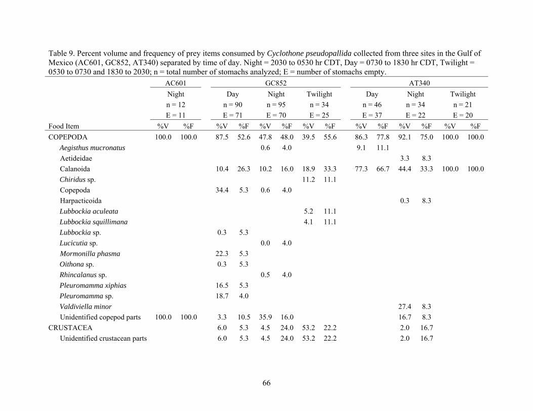
Table 12. Percent volume and frequency of prey items consumed by Diaphus mollis collected from three sites in the Gulf of Mexico (AC601, GC852, AT340) separated by time of day. Night = 2030 to 0530 hr CDT, Day = 0730 to 1830 hr CDT, Twilight = 0530 to 0730 and 1830 to 2030; n = total number of stomachs analyzed; E = number of stomachs empty. AC601 GC852 AT340 Night Day Night Twilight Day Night Twilight n = 1 n = 0 n = 14 n = 3 n = 4 n = 10 n = 2 E = 0 E = 0 E = 0 E = 2 E = 0 E = 1 E = 0 Food Item %V %F %V %F %V %F %V %F %V %F %V %F %V %F CHAETOGNATHA 28.1 25.0 8.4 11.1

Sagittoidea 8.4 11.1 Unidentified chaetognath parts 28.1 25.0

COPEPODA 63.4 100.0 15.3 57.1 12.8 100.0 12.5 25.0 20.9 77.8 79.0 100.0 Calanoida 12.5 25.0 <0.1 11.1 Copepoda 0.5 100.0 1.1 21.4 1.5 22.2 Cyclopoida 0.5 100.0 1.3 50.0 0.2 22.2 0.2 50.0

Farranula gracilis 0.2 11.1 Pleuromamma sp. 62.3 100.0 9.3 7.1 11.6 22.2 78.7 50.0

Unidentified copepod parts 3.7 21.4 12.8 100.0 7.4 44.4 0.1 50.0 CRUSTACEA 36.6 100.0 4.8 50.0 12.8 100.0 17.0 55.6 9.8 50.0

Unidentified crustacean parts 36.6 100.0 4.8 50.0 12.8 100.0 17.0 55.6 9.8 50.0 DECAPODA 0.1 11.1

Decapoda <0.1 7.1 0.1 11.1 EUPHAUSIACEA 34.4 25.0

Euphausiidae 34.4 25.0 FISH <0.1 21.4

Unidentified fish parts <0.1 21.4 MOLLUSCA 0.1 11.1

Gastropoda 0.1 11.1

71

Table 12 cont. OSTRACODA 1.4 50.0 6.4 100.0 <0.1 11.1 9.8 50.0

Conchoecinae 9.8 50.0 Myodocopida <0.1 14.3 6.4 100.0 Ostracoda 0.4 14.3 Unidentified ostracod parts 0.9 28.6 <0.1 11.1

OTHER <0.1 100.0 78.5 85.7 68.1 100.0 25.0 25.0 53.5 77.8 1.4 100.0 Organic material 78.4 85.7 68.0 100.0 25.0 25.0 53.5 77.8 1.4 100.0 Nematoda <0.1 100.0 <0.1 7.1 0.1 100.0 Unidentified animal parts <0.1 14.3 <0.1 11.1

72

Table 13. Percent volume and frequency of prey items consumed by Cyclothone pallida collected from three sites in the Gulf of Mexico (AC601, GC852, AT340) separated by time of day. Night = 2030 to 0530 hr CDT, Day = 0730 to 1830 hr CDT, Twilight = 0530 to 0730 and 1830 to 2030; n = total number of stomachs analyzed; E = number of stomachs empty. AC601 GC852 AT340 Night Day Night Twilight Day Night Twilight n = 18 n = 115 n = 95 n = 32 n = 58 n = 40 n = 4 E = 15 E = 109 E = 84 E = 32 E = 58 E = 39 E = 4 Food Item %V %F %V %F %V %F %V %F %V %F %V %F %V %F AMPHIPODA 29.9 9.09

Unidentified amphipod parts 29.9 9.09 COPEPODA 68.4 33.3 71.6 16.7 3.11 9.09

Aetideidae 22.6 16.7 Haloptilus oxycephalus 3.11 9.09

Unidentified copepod parts 68.4 33.3 49.0 16.7 CRUSTACEA 9.4 16.7

Unidentified crustacean parts 9.4 16.7 OSTRACODA 23.1 33.3 9.4 33.3 24.9 18.2

Conchoecinae 5.7 16.7 Halocyprididae 23.1 33.3 3.8 16.7 Myodocopida 9.96 9.09 Unidentified ostracod parts 14.9 9.09

OTHER 8.5 33.3 9.5 33.3 42.1 63.6 100.0 100.0 Organic material 8.5 33.3 9.5 33.3 42.1 63.6 100.0 100.0

73

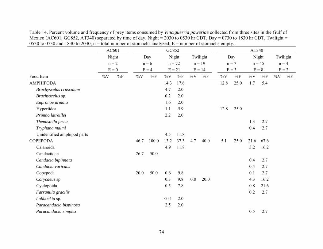
Table 14. Percent volume and frequency of prey items consumed by Vinciguerria poweriae collected from three sites in the Gulf of Mexico (AC601, GC852, AT340) separated by time of day. Night = 2030 to 0530 hr CDT, Day = 0730 to 1830 hr CDT, Twilight = 0530 to 0730 and 1830 to 2030; n = total number of stomachs analyzed; E = number of stomachs empty. AC601 GC852 AT340 Night Day Night Twilight Day Night Twilight n = 2 n = 6 n = 72 n = 19 n = 7 n = 45 n = 4 E = 0 E = 4 E = 21 E = 14 E = 3 E = 8 E = 2 Food Item %V %F %V %F %V %F %V %F %V %F %V %F %V %F AMPHIPODA 14.3 17.6 12.8 25.0 1.7 5.4 Brachyscelus crusculum 4.7 2.0 Brachyscelus sp. 0.2 2.0 Eupronoe armata 1.6 2.0

Hyperiidea 1.1 5.9 12.8 25.0 Primno latreillei 2.2 2.0 Themistella fusca 1.3 2.7 Tryphana malmi 0.4 2.7

Unidentified amphipod parts 4.5 11.8 COPEPODA 46.7 100.0 13.2 37.3 4.7 40.0 5.1 25.0 21.6 67.6

Calanoida 4.9 11.8 3.2 16.2 Candaciidae 26.7 50.0

Candacia bipinnata 0.4 2.7 Candacia varicans 0.4 2.7

Copepoda 20.0 50.0 0.6 9.8 0.1 2.7 Corycaeus sp. 0.3 9.8 0.8 20.0 4.3 16.2

Cyclopoida 0.5 7.8 0.8 21.6 Farranula gracilis 0.2 2.7 Lubbockia sp. <0.1 2.0 Paracandacia bispinosa 2.5 2.0 Paracandacia simplex 0.5 2.7

74

Table 14 cont. Pleuromamma sp. 3.9 20.0 Sapphirina sp. 0.1 2.0 Temora sp. <0.1 2.7 Undinula vulgaris 0.5 2.7

Unidentified copepod parts 4.3 21.6 5.1 25.0 11.1 54.1 CRUSTACEA 100.0 100.0 21.6 58.8 7.0 20.0 48.9 73.0

Unidentified crustacean parts 100.0 100.0 21.6 58.8 7.0 20.0 48.9 73.0 DECAPODA 12.6 2.0 0.7 2.7

Decapoda 12.6 2.0 Unidentified decapod parts 0.7 2.7

EUPHAUSIACEA 0.1 2.7 88.2 50.0Euphausiidae 0.1 2.7 88.2 50.0

FISH 53.3 50.0 12.2 3.9 67.4 60.0 0.1 2.7 Myctophidae 12.1 2.0 54.7 20.0 Unidentified fish parts 53.3 50.0 0.1 2.0 12.7 40.0 0.1 2.7

MOLLUSCA 0.1 2.0 Gastropoda 0.1 2.0

OSTRACODA 11.2 41.2 19.3 60.0 82.0 100.0 18.1 29.7 11.0 50.0Archiconchoecinae 0.8 2.0 0.5 20.0 1.8 5.4 Conchoecinae 4.8 13.7 18.8 40.0 13.6 50.0 7.6 8.1 Halocyprididae 1.4 3.9 68.5 50.0 1.8 5.4 11.0 50.0Halocypridinae 0.7 5.9

Halocypris sp. 0.6 3.9 Myodocopida 0.9 11.8 0.4 8.1 Myodocopina 1.1 5.4 Sarsiellidae 0.2 2.7 Unidentified ostracod parts 2.0 13.7 5.2 21.6

75

Table 14 cont. OTHER 14.9 35.3 1.6 20.0 8.8 21.6 0.8 50.0

Organic material 14.8 33.3 1.6 20.0 8.8 18.9 0.8 50.0Unidentified animal parts <0.1 7.8 <0.1 2.7

76

Table 15. Percent volume and frequency of prey items consumed by Myctophum affine collected from three sites in the Gulf of Mexico (AC601, GC852, AT340) separated by time of day. Night = 2030 to 0530 hr CDT, Day = 0730 to 1830 hr CDT, Twilight = 0530 to 0730 and 1830 to 2030; n = total number of stomachs analyzed; E = number of stomachs empty. AC601 GC852 AT340 Night Day Night Twilight Day Night Twilight n = 1 n = 10 n = 40 n = 6 n = 0 n = 4 n = 0 E = 0 E = 9 E = 21 E = 2 E = 0 E = 0 E = 0 Food Item %V %F %V %F %V %F %V %F %V %F %V %F %V %F AMPHIPODA 48.2 15.8 26.0 25.0 26.0 25.0

Amphipoda 25.4 5.3 Hyperiidea 7.6 5.3

Paratyphis sp. 15.2 5.3 Unidentified amphipod parts 26.0 25.0 26.0 25.0

CHAETOGNATHA 6.2 25.0 Unidentified chaetognath parts 6.2 25.0

COPEPODA 70.4 100 100.0 100 18.6 68.4 15.2 75.0 10.7 75.0 Calanoida 2.5 31.6 Candaciidae 6.9 5.3 Copepoda 0.4 10.5 Corycaeidae 0.7 100 <0.1 10.5 Cyclopoida 52.3 100.0 3.4 21.1 12.0 50.0 0.2 25.0

Farranula gracilis 0.3 15.8 Microsetella rosea 0.2 25.0

Oncaeidae 3.9 25.0 Temora sp. 17.4 100.0 0.4 5.3

Unidentified copepod parts 100.0 100 4.6 36.8 3.3 25.0 6.6 50.0 CRUSTACEA 6.2 47.4 24.5 25.0 3.9 50.0

Unidentified crustacean parts 6.2 47.4 24.5 25.0 3.9 50.0

77

Table 15 cont. DECAPODA 1.5 50.0

Decapoda 1.5 50.0 MOLLUSCA 10.9 25.0

Gastropoda 10.9 25.0 OSTRACODA 10.0 21.1 11.6 25.0

Conchoecinae 0.1 5.3 Halocyprididae <0.1 5.3 Myodocopida 9.8 5.3 Ostracoda <0.1 5.3 11.6 25.0

OTHER 29.6 100.0 17.0 52.6 49.5 50.0 40.1 75.0 Animalia <0.1 5.3 Organic material 26.1 100.0 16.9 47.4 49.5 50.0 40.1 75.0 Phytoplankton 0.1 5.3 Unidentified animal parts 3.5 100.0 <0.1 5.3

78

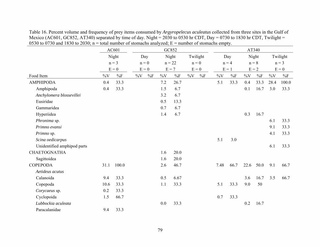
Table 16. Percent volume and frequency of prey items consumed by Argyropelecus aculeatus collected from three sites in the Gulf of Mexico (AC601, GC852, AT340) separated by time of day. Night = 2030 to 0530 hr CDT, Day = 0730 to 1830 hr CDT, Twilight = 0530 to 0730 and 1830 to 2030; n = total number of stomachs analyzed; E = number of stomachs empty. AC601 GC852 AT340 Night Day Night Twilight Day Night Twilight n = 3 n = 0 n = 22 n = 0 n = 4 n = 8 n = 3 E = 0 E = 0 E = 7 E = 0 E = 1 E = 2 E = 0 Food Item %V %F %V %F %V %F %V %F %V %F %V %F %V %F AMPHIPODA 0.4 33.3 7.2 26.7 5.1 33.3 0.4 33.3 28.4 100.0

Amphipoda 0.4 33.3 1.5 6.7 0.1 16.7 3.0 33.3 Anchylomera blossevillei 3.2 6.7

Eusiridae 0.5 13.3 Gammaridea 0.7 6.7 Hyperiidea 1.4 6.7 0.3 16.7

Phronima sp. 6.1 33.3 Primno evansi 9.1 33.3 Primno sp. 4.1 33.3 Scina oedicarpus 5.1 3.0

Unidentified amphipod parts 6.1 33.3 CHAETOGNATHA 1.6 20.0

Sagittoidea 1.6 20.0 COPEPODA 31.1 100.0 2.6 46.7 7.48 66.7 22.6 50.0 9.1 66.7 Aetideus acutus

Calanoida 9.4 33.3 0.5 6.67 3.6 16.7 3.5 66.7 Copepoda 10.6 33.3 1.1 33.3 5.1 33.3 9.0 50

Corycaeus sp. 0.2 33.3 Cyclopoida 1.5 66.7 0.7 33.3

Lubbockia aculeata 0.0 33.3 0.2 16.7 Paracalanidae 9.4 33.3

79

Table 16 cont. Paracalanus aculeatus 0.5 33.3 Pleuromamma robusta 2.0 33.3 Pleuromamma xiphias 9.8 16.7

Poecilostomatoida 0.3 33.3 1.5 33.3 Unidentified copepod parts 0.1 66.7 1.7 33.3 2.0 33.3

CRUSTACEA 1.8 33.3 33.4 80.0 17.7 66.7 31.1 83.3 13.7 66.7 Crustacea 1.9 13.3 0.3 16.7 Unidentified crustacean parts 1.8 33.3 31.5 80.0 17.7 66.7 30.9 83.3 13.7 66.7

DECAPODA 0.1 6.7 Unidentified decapod parts 0.1 6.7

EUPHAUSIACEA 14.2 20.0 Euphausiidae 14.2 20.0

MOLLUSCA 0.1 6.7 3.4 33.3 13.7 66.7 Gastropoda 0.1 6.7 3.4 33.3 3.6 66.7 Unidentified cephalopod parts 10.1 33.3

OSTRACODA 42.1 100.0 9.4 53.3 59.5 100.0 19.0 50.0 16.7 66.7 Archiconchoecinae 0.2 6.7 Conchoecinae 25.1 66.7 3.5 20.0 23.8 66.7 6.7 16.7 16.2 66.7 Halocypridinae 23.8 33.3

Halocypris sp. 4.6 33.3 Myodocopida 12.4 33.3 2.4 26.7 11.9 33.3 11.2 33.3 Ostracoda 2.7 6.7 Unidentified ostracod parts 0.6 20.0 1.1 16.7 0.5 33.3

OTHER 24.7 33.3 31.5 60.0 6.8 33.3 26.9 83.3 18.4 66.7 Organic material 24.7 33.3 25.6 60.0 6.8 33.3 26.9 83.3 18.3 66.7 Unidentified animal parts 5.9 6.7 0.2 33.3

80

Table 17. Percent volume and frequency of prey items consumed by Argyropelecus hemigymnus collected from three sites in the Gulf of Mexico (AC601, GC852, AT340) separated by time of day. Night = 2030 to 0530 hr CDT, Day = 0730 to 1830 hr CDT, Twilight = 0530 to 0730 and 1830 to 2030; n = total number of stomachs analyzed; E = number of stomachs empty. AC601 GC852 AT340 Night Day Night Twilight Day Night Twilight n = 1 n = 2 n = 8 n = 7 n = 3 n = 6 n = 3 E = 1 E = 0 E = 5 E = 4 E = 1 E = 5 E = 3 Food Item %V %F %V %F %V %F %V %F %V %F %V %F %V %FAMPHIPODA 0.9 50.0

Unidentified amphipod parts 0.9 50.0 COPEPODA 38.8 100.0 19.4 100.0 48.6 100.0 52.3 100.0 25.9 100.0

Calanoida 11.9 50.0 17.6 66.7 40.3 66.7 3.3 100.0 18.5 100.0 Copepoda 26.8 50.0 0.1 33.3 0.8 66.7 48.6 50.0

Lubbockia aculeata 4.94 100.0 Lubbockia sp. 0.7 33.3 Pleuromamma abdominalis 6.7 33.3

Unidentified copepod parts 1.7 33.3 0.3 50.0 2.47 100.0 CRUSTACEA 0.1 50.0 3.5 66.7 13.6 66.7 3.0 50.0

Crustacea 0.1 50.0 0.1 33.3 Unidentified crustacean parts 3.5 66.7 13.5 66.7 3.0 50.0

EUPHAUSIACEA 55.0 33.3 Nematoscelis microps 55.0 33.3 OSTRACODA 47.7 50.0 10.0 66.7 1.2 100.0

Conchoecinae 47.7 50.0 Myodocopida 6.6 33.3 Ostracoda 2.2 33.3 0.6 50.0 Unidentified ostracod parts 1.2 66.7 0.6 50.0

OTHER 13.4 100.0 12.1 100.0 37.8 100.0 42.6 100.0 74.1 100.0 Organic material 13.4 100.0 12.1 100.0 37.8 100.0 42.6 100.0 74.1 100.0

81

Table 18. Percent volume and frequency of prey items consumed by Pollichthys mauli collected from three sites in the Gulf of Mexico (AC601, GC852, AT340) separated by time of day. Night = 2030 to 0530 hr CDT, Day = 0730 to 1830 hr CDT, Twilight = 0530 to 0730 and 1830 to 2030; n = total number of stomachs analyzed; E = number of stomachs empty. AC601 GC852 AT340 Night Day Night Twilight Day Night Twilight n = 0 n = 0 n = 2 n = 0 n = 15 n = 21 n = 25 E = 0 E = 0 E = 0 E = 0 E = 6 E = 4 E = 5 Food Item %V %F %V %F %V %F %V %F %V %F %V %F %V %F AMPHIPODA 63.5 50.0 16.0 5.0

Amphipoda 16.0 5.0 Unidentified amphipod parts 63.5 50.0

COPEPODA 8.7 50.0 79.8 77.8 7.3 41.2 32.6 35.0 Calanoida 40.4 11.1 5.7 10.0 Copepoda 0.8 50.0 0.1 11.8 2.4 5.0

Corycaeus sp. 0.7 5.9 Cyclopoida 0.0 5.9 10.0 5.0 Harpacticoida 0.2 5.9

Pleuromamma borealis 4.5 5.9 Pleuromamma piseki 3.0 5.0 Pleuromamma sp. 1.4 5.9 10.4 10.0

Unidentified copepod parts 7.9 50.0 39.5 66.7 0.5 11.8 1.0 10.0 CRUSTACEA 11.9 58.8 10.1 55.0

Unidentified crustacean parts 11.9 58.8 10.1 55.0 DECAPODA 0.0 5.9

Unidentified decapod parts 0.0 5.9 EUPHAUSIACEA 61.6 17.6

Euphausiidae 0.1 5.9 Nyctiphanes capensis 24.0 5.9 Stylocheiron sp. 9.0 5.9

82

Table 18 cont. Thysanopoda sp. 28.5 5.9 OSTRACODA 27.8 50.0 17.9 11.1 15.0 29.4 38.1 35.0

Conchoecinae 11.9 50.0 12.7 11.8 18.0 15.0 Halocyprididae 7.8 10.0 Myodocopida 0.0 11.8 Ostracoda 17.9 11.1 1.8 11.8 7.8 20.0 Unidentified ostracod parts 15.9 50.0 0.5 11.8 4.4 10.0

OTHER 2.2 11.1 4.2 17.6 3.2 20.0 Organic material 2.2 11.1 4.2 17.6 3.2 20.0

83

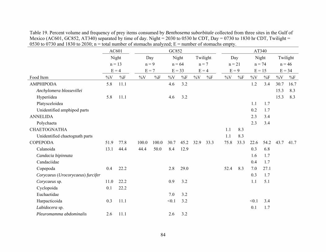
Table 19. Percent volume and frequency of prey items consumed by Benthosema suborbitale collected from three sites in the Gulf of Mexico (AC601, GC852, AT340) separated by time of day. Night = 2030 to 0530 hr CDT, Day = 0730 to 1830 hr CDT, Twilight = 0530 to 0730 and 1830 to 2030; n = total number of stomachs analyzed; E = number of stomachs empty. AC601 GC852 AT340 Night Day Night Twilight Day Night Twilight n = 13 n = 9 n = 64 n = 7 n = 21 n = 74 n = 46 E = 4 E = 7 E = 33 E = 4 E = 9 E = 15 E = 34 Food Item %V %F %V %F %V %F %V %F %V %F %V %F %V %F AMPHIPODA 5.8 11.1 4.6 3.2 1.2 3.4 30.7 16.7 Anchylomera blossevillei 15.3 8.3

Hyperiidea 5.8 11.1 4.6 3.2 15.3 8.3 Platysceloidea 1.1 1.7 Unidentified amphipod parts 0.2 1.7

ANNELIDA 2.3 3.4 Polychaeta 2.3 3.4


COPEPODA 51.9 77.8 100.0 100.0 30.7 45.2 32.9 33.3 75.8 33.3 22.6 54.2 43.7 41.7 Calanoida 13.1 44.4 44.4 50.0 8.4 12.9 0.3 6.8

Candacia bipinnata 1.6 1.7 Candaciidae 0.4 1.7 Copepoda 0.4 22.2 2.8 29.0 52.4 8.3 7.0 27.1

Corycaeus (Urocorycaeus) furcifer 0.3 1.7 Corycaeus sp. 11.0 22.2 0.9 3.2 1.1 5.1

Cyclopoida 0.1 22.2 Euchaetidae 7.0 3.2 Harpacticoida 0.3 11.1 <0.1 3.2 <0.1 3.4

Labidocera sp. 0.1 1.7 Pleuromamma abdominalis 2.6 11.1 2.6 3.2

84

Table 19 cont. Pleuromamma borealis 2.1 1.7 9.2 8.3 Pleuromamma piseki 10.3 22.2 Pleuromamma sp. 55.6 50.0 7.0 3.2 1.4 1.7 10.2 8.3 Sapphirina metallina 2.1 11.1 Temora stylifera 3.4 11.1

Unidentified copepod parts 8.6 33.3 2.0 12.9 32.9 33.3 23.4 25.0 8.3 32.2 24.2 33.3 CRUSTACEA 24.3 44.4 17.9 38.7 7.9 66.7 11.2 8.3 19.9 49.2 8.4 33.3

Crustacea 0.2 3.2 Unidentified crustacean parts 24.3 44.4 17.7 38.7 7.9 66.7 11.2 8.3 19.9 49.2 8.4 33.3

DECAPODA 21.5 3.2 5.2 5.1 Decapoda 21.5 3.2 2.8 1.7 Unidentified decapod parts 2.3 3.4

EUPHAUSIACEA 0.1 3.2 11.7 3.4 Euphausiidae 0.1 3.2 11.7 3.4

FISH 8.5 1.7 Myctophidae 8.5 1.7

OSTRACODA 2.7 33.3 7.2 25.8 3.0 16.7 5.0 20.3 1.3 8.3 Archiconchoecinae 2.1 1.7 Conchoecinae 2.1 6.5 Halocyprididae 1.8 3.2

Halocypris sp. 1.8 3.2 Myodocopida 1.8 22.2 0.8 9.7 0.3 5.1 Ostracoda 0.9 11.1 3.0 16.7 0.3 3.4 1.3 8.3 Unidentified ostracod parts 0.8 6.5 2.3 13.6

OTHER 15.4 55.6 18.0 45.2 59.2 66.7 8.8 33.3 23.5 67.8 15.9 58.3 Organic material 15.4 55.6 18.0 45.2 59.2 66.7 7.9 25.0 23.5 66.1 15.9 58.3 Unidentified animal parts <0.1 3.2 0.9 8.3 <0.1 1.7

85

Table 20. Percent volume and frequency of prey items consumed by Lampanyctus alatus collected from three sites in the Gulf of Mexico (AC601, GC852, AT340) separated by time of day. Night = 2030 to 0530 hr CDT, Day = 0730 to 1830 hr CDT, Twilight = 0530 to 0730 and 1830 to 2030; n = total number of stomachs analyzed; E = number of stomachs empty. AC601 GC852 AT340 Night Day Night Twilight Day Night Twilight n = 6 n = 5 n = 25 n = 12 n = 3 n = 16 n = 5 E = 0 E = 3 E = 4 E = 4 E = 0 E = 4 E = 0 Food Item %V %F %V %F %V %F %V %F %V %F %V %F %V %F AMPHIPODA 30.4 33.3 20.1 23.8 28.4 12.5

Amphipoda 1.8 14.3 Gammaridea 0.1 4.8 Hyperiidea 27.2 16.7

Lestrigonus sp. 3.3 4.8 Unidentified amphipod parts 3.1 16.7 14.9 4.8 28.4 12.5

COPEPODA 34.9 83.3 28.3 100 20.3 52.4 7.8 37.5 59.2 100.0 22.5 66.7 15.4 40.0 Aetideus acutus

Calanoida 10.9 33.3 26.1 100.0 0.7 9.5 55.0 66.7 0.6 16.7 15.4 40.0 Candacia longimana

Copepoda 0.1 19.0 2.4 12.5 8.1 33.3 Corycaeus sp. 0.5 4.8 Eucalanus sp. 5.9 4.8 Oncaea sp. 2.2 50.0 Paracandacia simplex 4.3 33.3 Pleuromamma piseki 8.4 8.3 Pleuromamma sp. 6.2 16.7 0.9 9.5 2.7 8.3

Unidentified copepod parts 17.8 50.0 12.1 23.8 5.4 37.5 2.7 16.7 CRUSTACEA 22.4 33.3 60.9 50.0 40.0 47.6 60.8 50.0 40.8 33.3 28.5 83.3

Crustacea 0.1 4.8

86

Table 20 cont. Unidentified crustacean parts 22.4 33.3 60.9 50.0 40.0 42.9 60.8 50.0 40.8 33.3 28.5 83.3

DECAPODA 4.5 4.8 Decapoda 4.5 4.8


Nematoscelis sp. 5.8 4.8 FISH <0.1 4.8

Unidentified fish parts <0.1 4.8 OSTRACODA 7.6 33.3 4.7 38.1 1.9 25.0 1.3 25.0

Conchoecinae 6.8 16.7 3.6 9.5 Halocyprididae 0.8 33.3 0.3 4.8 Myodocopida <0.1 4.8 1.3 16.7 Ostracoda 0.4 9.5 Unidentified ostracod parts 0.4 9.5 1.9 25.0 <0.1 8.3

SALPIDA 10.9 50.0 Salpidae 10.9 50.0

OTHER 4.7 16.7 4.5 28.6 1.1 37.5 25.9 50.0 84.6 60.0Organic material 4.7 16.7 4.2 23.8 1.1 37.5 25.9 50.0 84.6 60.0Nematoda 0.3 4.8

87

Table 21. Percent volume and frequency of prey items consumed by Lepidophanes guentheri collected from three sites in the Gulf of Mexico (AC601, GC852, AT340) separated by time of day. Night = 2030 to 0530 hr CDT, Day = 0730 to 1830 hr CDT, Twilight = 0530 to 0730 and 1830 to 2030; n = total number of stomachs analyzed; E = number of stomachs empty. AC601 GC852 AT340 Night Day Night Twilight Day Night Twilight n = 15 n = 4 n = 36 n = 7 n = 25 n = 57 n = 13 E = 0 E = 1 E = 11 E = 2 E = 8 E = 9 E = 7 Food Item %V %F %V %F %V %F %V %F %V %F %V %F %V %F AMPHIPODA 39.3 8.0 10.9 5.9 0.2 2.1

Amphipoda Gammaridea Hyperiidea 6.5 4.0

Phronima sp. 32.7 4.0 Unidentified amphipod parts 10.9 5.9 0.2 2.1

COPEPODA 75.9 86.7 12.1 66.7 28.5 76.0 <0.1 20.0 10.7 53.3 24.2 62.5 22.9 50.0 Aetideus acutus

Calanoida 27.6 20.0 3.65 33.3 10.0 12.0 2.2 11.8 6.2 16.7 17.4 16.7 Candacia curta 0.6 2.1 Candacia sp. 3.9 4.0

Copepoda 2.2 26.7 0.3 12.0 0.9 12.5 Corycaeus sp. 0.3 4.0

Cyclopoida 0.2 33.3 0.5 24.0 <0.1 20.0 <0.1 6.3 Farranula gracilis <0.1 2.1

Harpacticoida 0.1 4.0 0.5 5.9 Oncaea sp. Paracandacia simplex Pleuromamma gracilis 0.3 4.0 Pleuromamma piseki 14.2 6.7 3.3 4.0 9.3 12.5 Pleuromamma sp. 7.3 26.7 6.1 10.4

88

Table 21 cont. Unidentified copepod parts 24.4 53.3 8.47 33.3 9.7 40.0 8.0 29.4 1.1 16.7 5.5 33.3

CRUSTACEA 6.2 13.3 17.7 28.0 80.3 40.0 36.8 17.6 54.6 47.9 20.9 16.7 Crustacea Unidentified crustacean parts 6.2 13.3 17.7 28.0 80.3 40.0 36.8 17.6 54.6 47.9 20.9 16.7

DECAPODA 0.3 4.0 0.3 10.4 Decapoda 0.3 4.0 Unidentified decacod parts 0.3 10.4

EUPHAUSIACEA 14.9 33.3 28.4 11.8 11.1 4.2 Euphausiidae 14.9 33.3 28.4 11.8 9.3 2.1

Thysanopoda sp. 1.8 2.1 FISH <0.1 4.0 <0.1 2.1

Unidentified fish parts <0.1 4.0 <0.1 2.1 MOLLUSCA 0.9 2.1

Gastropoda 0.9 2.1 OSTRACODA 8.3 60 71.1 33.3 9.6 36 1.8 20.8 16.7 16.7

Conchoecinae 0.2 13.3 71.1 33.3 7.6 16.0 0.6 2.1 Halocyprididae 2.4 6.7 Myodocopida 0.5 20.0 1.2 12.0 16.7 16.7 Ostracoda 0.3 4.0 0.1 8.3 Unidentified ostracod parts 5.2 40.0 0.5 12.0 1.1 10.4

SALPIDA Salpidae

OTHER 9.6 53.3 1.86 33.3 4.7 48.0 19.7 80.0 13.2 35.3 6.9 35.4 39.4 50.0 Organic material 9.6 46.7 1.86 33.3 4.7 40.0 19.6 60.0 13.2 35.3 6.9 35.4 39.4 50.0 Nematoda <0.1 6.7 <0.1 8.0 0.1 40.0

89

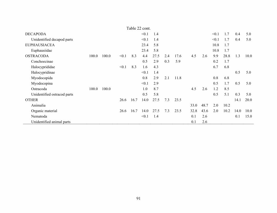
Table 22. Percent volume and frequency of prey items consumed by Notolychnus valdiviae collected from three sites in the Gulf of Mexico (AC601, GC852, AT340) separated by time of day. Night = 2030 to 0530 hr CDT, Day = 0730 to 1830 hr CDT, Twilight = 0530 to 0730 and 1830 to 2030; n = total number of stomachs analyzed; E = number of stomachs empty. AC601 GC852 AT340 Night Day Night Twilight Day Night Twilight n = 1 n = 14 n = 92 n = 30 n = 71 n = 94 n = 41 E = 0 E = 2 E = 23 E = 13 E = 32 E = 35 E = 21 Food Item %V %F %V %F %V %F %V %F %V %F %V %F %V %F CHAETOGNATHA <0.1 5.9

Unidentified chaetognath parts <0.1 5.9 COPEPODA 22.3 33.3 39.4 52.2 36.0 41.2 62.4 61.5 52.3 67.8 72.8 55.0

Calanoida <0.1 8.3 18.1 20.3 3.3 5.9 4.3 10.3 8.5 13.6 1.7 5.0 Candaciidae 0.9 5.9 1.5 2.6 Copepoda 0.1 5.9 4.1 2.6 Corycaeidae 0.2 3.4 Cyclopoida <0.1 5.8 <0.1 2.6 1.4 18.6

Euchaeta sp. 14.1 8.3 Harpacticoida <0.1 5.0

Lubbockia squillimana <0.1 1.4 Oncaea sp. 0.1 2.9 0.2 3.4 0.3 5.0 Paracandacia simplex 2.7 2.6 Pleuromamma gracilis 0.4 1.4 Pleuromamma piseki 3.0 1.4 0.9 2.6 Pleuromamma sp. 0.8 2.9 32.0 10.3 6.1 5.1 17.1 15.0 Pleuromamma xiphias 12.6 4.3 20.5 5.1 5.3 5.0

Poecilostomatoida 0.5 5.9 0.6 1.7 Unidentified copepod parts 8.2 16.7 4.2 23.2 31.1 29.4 16.8 30.8 14.8 23.7 48.5 25.0

CRUSTACEA 51.0 58.3 18.7 43.5 54.3 58.8 0.1 2.6 25.0 33.9 11.3 25.0Unidentified crustacean parts 51.0 58.3 18.7 43.5 54.3 58.8 0.1 2.6 25.0 33.9 11.3 25.0

90

Table 22 cont. DECAPODA <0.1 1.4 <0.1 1.7 0.4 5.0

Unidentified decapod parts <0.1 1.4 <0.1 1.7 0.4 5.0 EUPHAUSIACEA 23.4 5.8 10.8 1.7

Euphausiidae 23.4 5.8 10.8 1.7 OSTRACODA 100.0 100.0 <0.1 8.3 4.4 27.5 2.4 17.6 4.5 2.6 9.9 28.8 1.3 10.0

Conchoecinae 0.5 2.9 0.3 5.9 0.2 1.7 Halocyprididae <0.1 8.3 1.6 4.3 6.7 6.8 Halocypridinae <0.1 1.4 0.5 5.0 Myodocopida 0.8 2.9 2.1 11.8 0.8 6.8 Myodocopina <0.1 2.9 0.5 1.7 0.5 5.0 Ostracoda 100.0 100.0 1.0 8.7 4.5 2.6 1.2 8.5 Unidentified ostracod parts 0.5 5.8 0.5 5.1 0.3 5.0

OTHER 26.6 16.7 14.0 27.5 7.3 23.5 14.1 20.0Animalia 33.0 48.7 2.0 10.2 Organic material 26.6 16.7 14.0 27.5 7.3 23.5 32.8 43.6 2.0 10.2 14.0 10.0Nematoda <0.1 1.4 0.1 2.6 0.1 15.0Unidentified animal parts 0.1 2.6

91

Table 23. Percent volume and frequency of prey items consumed by Ceratoscopelus warmingii collected from three sites in the Gulf of Mexico (AC601, GC852, AT340) separated by time of day. Night = 2030 to 0530 hr CDT, Day = 0730 to 1830 hr CDT, Twilight = 0530 to 0730 and 1830 to 2030; n = total number of stomachs analyzed; E = number of stomachs empty. AC601 GC852 AT340 Night Day Night Twilight Day Night Twilight n = 5 n = 6 n = 23 n = 5 n = 6 n = 39 n = 4 E = 1 E = 4 E = 4 E = 2 E = 3 E = 1 E = 1 Food Item %V %F %V %F %V %F %V %F %V %F %V %F %V %F AMPHIPODA 54.6 50.0 8.8 31.6 0.4 33.3 0.8 13.2

Amphipoda 54.6 50.0 0.7 10.5 0.6 13.2 Hyperiidea 1.7 10.5 0.4 33.3 0.2 2.63

Phronima stebbingii 4.9 5.3 Unidentified amphipod parts 1.5 15.8

ANNELIDA 1.7 15.8 0.2 33.3 1.5 7.89 Unidentified polychaete parts 1.7 15.8 0.2 33.3 1.5 7.89


CNIDARIA 1.8 2.63 Hydrozoa 1.8 2.63

COPEPODA 34.6 100.0 3.7 47.4 1.2 66.7 13.4 100.0 9.5 65.8 2.3 66.7 Calanoida 2.4 25.0 2.6 5.3 0.3 33.3 0.7 33.3 1.0 5.26

Candacia sp. 3.5 33.3 Copepoda 0.8 26.3 0.8 33.3 2.8 55.3 0.4 66.7 Corycaeidae 0.6 33.3

Corycaeus sp. 12.7 75.0 0.2 5.3 0.1 2.63 1.9 33.3 Cyclopoida 0.0 5.3 0.0 2.63 Harpacticoida 0.1 2.63

Microsetella rosea 0.0 5.3 Miracia efferata 1.1 33.3

92

Table 23 cont. Miraciidae 0.0 2.63

Temora stylifera 0.4 33.3 Unidentified copepod parts 19.5 25.0 0.0 10.5 7.1 33.3 5.5 21.1

CRUSTACEA 46.8 50.0 3.6 36.8 16.7 66.7 8.4 33.3 2.7 31.6 Crustacea 0.3 5.3 0.1 2.63 Unidentified crustacean parts 46.8 50.0 3.3 31.6 16.7 66.7 8.4 33.3 2.6 31.6 38.7 66.7

DECAPODA 0.6 7.9 Caridea 0.1 2.63 Decapoda 0.2 2.63 Unidentified decapod parts 0.2 2.63


FISH 0.1 5.3 77.0 33.3 0.2 5.26 Unidentified fish parts 77.0 33.3 0.2 5.26

MOLLUSCA 6.9 10.5 1.1 7.89 52.5 33.3 Bivalvia 1.0 33.3 Cephalopoda 6.5 5.3 Gastropoda 1.1 7.89 51.6 33.3 Mollusca 0.4 5.3

OSTRACODA 5.9 25.0 3.9 31.6 5.6 33.3 2.4 34.2 Conchoecinae 0.3 2.63 Halocyprididae 0.2 2.63 Myodocopida 5.9 25.0 0.5 21.1 5.2 33.3 0.7 15.8 Ostracoda 0.1 5.3 0.4 33.3 0.9 10.5 Platycopida 0.1 2.63 Unidentified ostracod parts 3.3 10.5 0.2 7.89

SALPIDA 3.2 5.3 Salpida 3.2 5.3

93

Table 23 cont. OTHER 53.2 50.0 68.2 78.9 76.3 100.0 0.9 33.3 79.0 97.4 6.4 33.3

Organic material 53.2 50.0 65.0 73.7 76.3 100.0 0.9 33.3 73.5 94.7 Unidentified animal parts 3.2 10.5 5.4 10.5 6.4 33.3

94

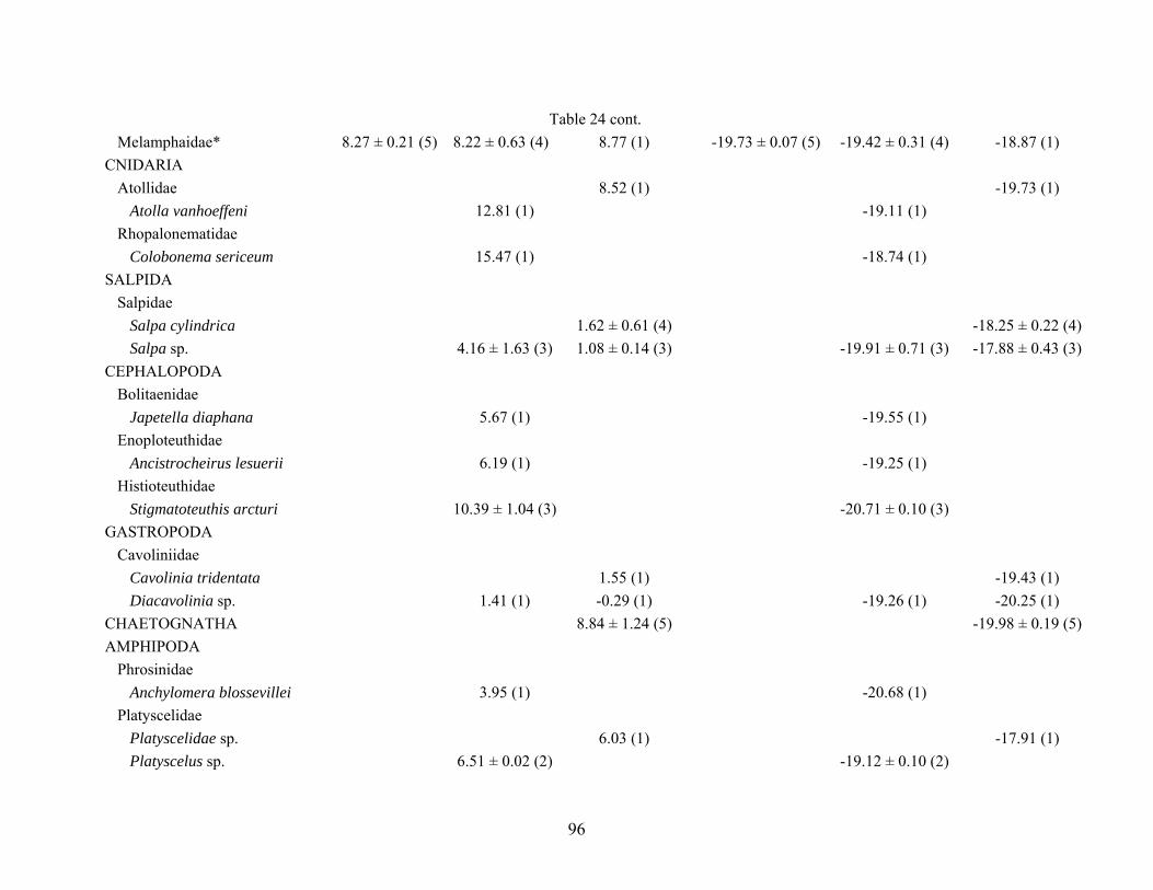
Table 24. Mean (± 1 standard error) δ13C and δ15N values for midwater fishes, invertebrates and carbon sources collected from each site (AC601, AT340, GC852). n = number in parentheses, * = multiple fish species grouped together δ15N δ13C Species AC601 GC852 AT340 AC601 GC852 AT340 FISH

Gonostomatidae Cyclothone acclinidens 9.52 (1) -18.45 (1) Cyclothone alba 7.32 ± 0.32 (5) -19.53 ± 0.12 (5) Cyclothone pallida 8.44 ± 0.28 (5) 9.97 (1) 8.56 ± 0.63 (4) -19.22 ± 0.12 (5) -18.10 (1) -18.82 ± 0.15 (4) Cyclothone pseudopallida 7.61 ± 0.17 (4) 7.82 ± 0.21 (3) 7.64 ± 0.28 (3) -19.48 ± 0.41 (4) -18.77 ± 0.29 (3) -18.74 ± 0.35 (3) Gonostoma elongatum 8.96 ± 0.27 (6) 7.22 ± 0.23 (6) -18.87 ± 0.31 (6) -18.84 ± 0.11 (6)

Sternoptychidae Argyropelecus aculeatus 7.90 ± 0.44 (5) 8.68 ± 0.24 (5) -18.83 ± 0.10 (5) -17.94 ± 0.41 (5) Argyropelecus hemigymnus 7.82 (1) 7.80 ± 0.22 (9) -18.63 (1) -18.72 ± 0.18 (9) Sternoptyx spp.* 8.60 ± 0.26 (7) 6.99 ± 0.89 (2) -19.75 ± 0.12 (7) -19.49 ± 0.16 (2) Valenciennellus tripunctulatus 9.15 ± 0.09 (5) 9.06 ± 0.21 (5) 8.57 ± 0.28 (5) -19.97 ± 0.14 (5) -19.73 ± 0.16 (5) -18.76 ± 0.41 (5)

Phosichthyidae Pollichthys mauli 6.60 ± 0.19 (10) -18.60 ± 0.10 (10) Vinciguerria poweriae 7.94 ± 0.10 (10) 7.59 ± 0.32 (5) -19.60 ± 0.09 (10) -18.98 ± 0.09 (5)

Stomiidae* 8.37 ± 0.26 (11) 7.90 ± 0.95 (6) -19.24 ± 0.32 (11) -18.86 ± 0.37 (6) Chauliodus sloani 8.03 ± 0.24 (5) 9.11 (1) -19.95 ± 0.54 (5) -17.92 (1)

Myctophidae Benthosema suborbitale 6.80 ± 0.42 (3) 7.26 ± 0.49 (3) -19.60 ± 0.30 (3) -18.57 ± 0.19 (3) Ceratoscopelus warmingii 6.36 ± 0.29 (3) 7.21 ± 0.33 (5) 6.43 ± 0.63 (4) -19.60 ± 0.26 (3) -19.34 ± 0.21 (5) -18.98 ± 0.35 (4) Diaphus spp.* 8.41 (1) 8.76 ± 0.71 (5) -19.18 (1) -19.33 ± 0.28 (5) Diaphus problematicus 9.20 (1) 7.97 ± 0.26 (6) -19.23 (1) -18.33 ± 0.08 (6) Lampanyctus alatus 7.91 ± 0.22 (3) 8.48 ± 0.19 (7) 7.49 ± 0.29 (5) -19.52 ± 0.22 (3) -19.51 ± 0.13 (7) -18.95 ± 0.19 (5) Lepidophanes guentheri 7.94 ± 0.25 (4) 6.75 ± 0.23 (6) -19.22 ± 0.10 (4) -18.42 ± 0.04 (6) Myctophum affine 5.87 ± 0.28 (10) -21.32 ± 0.22 (10)

95

Table 24 cont. Melamphaidae* 8.27 ± 0.21 (5) 8.22 ± 0.63 (4) 8.77 (1) -19.73 ± 0.07 (5) -19.42 ± 0.31 (4) -18.87 (1)

CNIDARIA Atollidae 8.52 (1) -19.73 (1)

Atolla vanhoeffeni 12.81 (1) -19.11 (1) Rhopalonematidae

Colobonema sericeum 15.47 (1) -18.74 (1) SALPIDA

Salpidae Salpa cylindrica 1.62 ± 0.61 (4) -18.25 ± 0.22 (4) Salpa sp. 4.16 ± 1.63 (3) 1.08 ± 0.14 (3) -19.91 ± 0.71 (3) -17.88 ± 0.43 (3)

CEPHALOPODA Bolitaenidae

Japetella diaphana 5.67 (1) -19.55 (1) Enoploteuthidae

Ancistrocheirus lesuerii 6.19 (1) -19.25 (1) Histioteuthidae

Stigmatoteuthis arcturi 10.39 ± 1.04 (3) -20.71 ± 0.10 (3) GASTROPODA

Cavoliniidae Cavolinia tridentata 1.55 (1) -19.43 (1) Diacavolinia sp. 1.41 (1) -0.29 (1) -19.26 (1) -20.25 (1)

CHAETOGNATHA 8.84 ± 1.24 (5) -19.98 ± 0.19 (5) AMPHIPODA

Phrosinidae Anchylomera blossevillei 3.95 (1) -20.68 (1)

Platyscelidae Platyscelidae sp. 6.03 (1) -17.91 (1) Platyscelus sp. 6.51 ± 0.02 (2) -19.12 ± 0.10 (2)

96

Table 24 cont. Pronoidae

Parapronoe sp. 7.59 (1) -19.33 (1) COPEPODA 3.70 (1) 7.00 ± 1.53 (5) -19.14 (1) -19.57 ± 0.32 (5)

Megacalanidae Bathycalanus princeps 9.06 ± 0.57 (4) -20.58 ± 0.34 (4)

Pontellidae Labidocera sp. 3.65 ± 0.29 (2) -18.96 ± 0.18 (2)

EUPHAUSIACEA 5.97 ± 0.66 (4) 6.65 ± 0.25 (2) 4.98 ± 0.23 (5) -19.57 ± 0.26 (4) -19.16 ± 0.002 (2) -19.14 ± 0.24 (5) Euphausiidae

Nematodcelis megalops 6.60 ± 0.33 (3) -19.50 ± 0.46 (3) Thysanopoda sp. 7.74 ± 0.61 (2) -19.10 ± 0.54 (2) Thysanopoda tricuspida 2.90 ± 0.50 (2) -17.74 ± 0.41 (2)

DECAPODA Benthesicymidae

Gennadas valens 6.83 ± 0.12 (4) 7.50 ± 0.32 (6) 6.49 ± 0.10 (4) -19.16 ± 0.39 (4) -18.47 ± 0.31 (6) -18.26 ± 0.14 (4) Oplophoridae

Acanthephyra purpurea 7.78 ± 0.63 (4) 6.98 (1) -17.50 ± 0.14 (4) -18.41 (1) Systellaspis debilis 6.30 (1) 5.93 ± 0.29 (6) -17.17 (1) -17.84 ± 0.07 (6)

Sergestidae Sergia sp. 7.79 (1) -19.10 (1)

ZOOPLANKTON 5.96 ± 2.17 (2) 7.43 ± 0.99 (5) 4.34 ± 1.36 (4) -19.19 ± 0.06 (2) -20.37 ± 0.70 (5) -19.57 ± 0.61 (4) AUTOTROPH

Sargassaceae Sargassum spp. 1.40 ± 0.33 (3) 1.88 ± 1.00 (5) -0.37 ± 0.41 (4) -17.48 ± 0.65 (3) -17.60 ± 1.05 (5) -18.48 ± 0.29 (4)

Detritus 3.60 ± 2.08 (5) -9.95 ± 0.92 (5) Phytoplankton 3.82 ± 0.57 (5) 2.36 ± 0.68 (8) 5.25 ± 0.35 (8) -20.01 ± 0.78 (5) -19.78 ± 0.83 (8) -19.36 ± 0.69 (8)

97

Table 25. Percent of prey contributions for each midwater fish species using IsoSource. *Results for M. affine are based on the inclusion of chemosynthetic material, as this species was not bound by the photosynthetic based prey sources. Zooplankton Cnidaria Pterapoda Salpida Cephalopoda Family Species 1-99 %ile 1-99 %ile 1-99 %ile 1-99 %ile 1-99 %ile Gonostomatidae Cyclothone alba 0.26-0.72 0-0.18 0.12-0.46 0-0.12 0-0.28 Cyclothone pallida 0-0.46 0-0.36 0-0.30 0-0.38 0-0.56 Cyclothone pseudopallida 0-0.50 0-0.28 0-0.42 0-0.46 0-0.46 Gonostoma elongatum 0-0.36 0-0.28 0-0.28 0-0.42 0-0.40 Sternoptychidae Argyropelecus aculeatus 0-0.14 0-0.14 0-0.16 0-0.28 0-0.18 Argyropelecus hemigymnus 0-0.30 0-0.26 0-0.30 0-0.50 0-0.34 Sternoptyx spp. 0.94-0.98 0.00 0.02-0.06 0.00 0-0.02 Valenciennellus tripunctulatus 0.18-0.78 0-0.34 0-0.32 0-0.12 0-0.52 Phosichthyidae Pollichthys mauli 0-0.18 0-0.16 0-0.36 0.08-0.66 0-0.22 Vinciguerria poweriae 0-0.64 0-0.26 0.02-0.44 0-0.22 0-0.42 Stomiidae Chauliodus sloani 0.48-0.90 0-0.10 0-0.20 0-0.06 0-0.18 Stomiidae 0-0.34 0-0.28 0-0.28 0-0.42 0-0.40 Myctophidae Benthosema suborbitale 0-0.46 0-0.24 0-0.5 0-0.50 0-0.38 Ceratoscopelus warmingii 0-0.44 0-0.28 0.08-0.54 0-0.36 0-0.32 Diaphus problematicus 0-0.18 0-0.16 0-0.20 0-0.34 0-0.22 Lampanyctus alatus 0-0.70 0-0.32 0-0.44 0-0.26 0-0.52 Lepidophanes guentheri 0-0.28 0-0.22 0-0.36 0-0.56 0-0.32 Myctophum affine* 0-0.28 0-0.12 0-0.42 0-0.42 0-0.20 Melamphaidae Melamphaidae 0.30-0.86 0-0.24 0-0.32 0-0.12 0-0.38

98

Table 25 cont. Decapoda Euphausiid Fish POM Chemo 1-99 %ile 1-99 %ile 1-99 %ile 1-99 %ile 1-99 %ile

0-0.06 0-0.28 0-0.48 0-0.56 0-0.38 0-0.64 0-0.52 0-0.52 0-0.38

0.52-0.84 0-0.24 0.06-0.62 0-0.46

0.00 0.00 0-0.10 0-0.34

0.06-0.50 0-0.30 0-0.14 0-0.50 0-0.52 0-0.04 0-0.16 0-0.34

0.02-0.58 0-0.58 0-0.28 0-0.34 0-0.58 0-0.20 0-0.48 0-0.38

0.42-0.78 0-0.28 0-0.18 0-0.64

0.02-0.54 0-046 0-0.24 0-0.32 0-0.50 0.22-0.300-0.08 0-0.34

99

100

Table 26. Mean trophic position (TP), one standard deviation (Stdev), range (minimum – maximum) and number of fish (n) for each midwater fish species collected in the north-central Gulf of Mexico, using data from stable isotope and gut content analyses. Trophic positions were calculated using modified equations from Vander Zanden et al. (1996) (see methods). GCA SIA Mean TP Stdev Range n Mean TP Stdev Range n Cyclothone alba 3.04 0.13 3.00 - 3.50 57 2.64 0.36 2.26 - 3.01 5 Cyclothone braueri 3.00 0.00 3.00 - 3.00 60 Cyclothone pallida 3.00 0.00 3.00 - 3.00 9 3.30 0.48 2.39 - 3.96 10 Cyclothone pseudopallida 3.01 0.07 3.00 - 3.50 51 2.82 0.18 2.57 - 3.07 10 Gonostoma elongatum 3.18 0.27 3.00 - 3.94 29 3.02 0.54 2.28 - 3.93 12 Argyropelecus aculeatus 3.07 0.15 3.00 - 3.50 25 3.12 0.43 2.08 - 3.59 10 Argyropelecus hemigymnus 3.03 0.12 3.00 - 3.38 11 2.88 0.31 2.46 - 3.23 10 Sternoptyx spp. 3.10 0.40 2.16 - 3.49 9 Valenciennellus tripunctulatus 3.01 0.05 3.00 - 3.49 87 3.44 0.26 2.74 - 3.82 15 Pollichthys mauli 3.06 0.15 3.00 - 3.50 34 2.28 0.30 1.85 - 2.78 10 Vinciguerria poweriae 3.07 0.21 3.00 - 4.00 69 2.89 0.24 2.39 - 3.22 15 Chauliodus sloani 4.00 0.00 4.00 - 4.00 5 3.09 0.32 2.73 - 3.83 6 Stomiidae 3.87 0.23 3.50 - 4.00 8 3.08 0.91 1.60 - 3.67 11 Benthosema suborbitale 3.06 0.19 3.00 - 4.00 83 2.50 0.37 2.05 - 2.93 6 Ceratoscopelus warmingii 3.14 0.27 2.90 - 4.00 56 2.35 0.46 1.57 - 2.94 12 Diaphus problematicus 3.05 0.37 2.67 - 3.58 7 Diaphus spp. 3.17 0.33 3.00 - 4.00 27 3.33 0.33 2.76 - 3.69 6 Hygophum benoiti 3.02 0.08 3.00 - 3.27 13 Lampanyctus alatus 3.04 0.13 3.00 - 3.50 46 3.00 0.34 2.44 - 3.55 15 Lepidophanes guentheri 3.05 0.14 2.94 - 3.50 91 2.59 0.40 1.90 - 3.16 10 Myctophum affine 3.05 0.20 2.99 - 4.00 24 1.92 0.44 1.19 - 2.48 10 Notolychnus valdiviae 3.04 0.14 3.00 - 4.00 151 Melamphaidae 3.13 0.41 2.51 - 3.65 10

Figure 1. Sampling areas in the North-central Gulf of Mexico for midwater fauna, 9-25 August 2007. The three cold seep sites (AT340, GC852, AC601) were located on the continental slope at depths > 1000 m. Each dot represents one station.

101

Figure 2. Multidimensional scaling (MDS) plot documenting the differences among the gut contents of midwater fishes. Data were based on the Bray-Curtis similarity matrix calculated from standardized, square root transformed, mean volumes of prey (12 general categories). Colors represent the different fish families, red = Gonostomatidae, Orange = Sternoptychidae, Green = Phosichthyidae, Blue = Stomiidae, Purple = Myctophidae. Ca = Cyclothone alba, Cb = Cyclothone braueri, Cp = Cyclothone pallida, Cps = Cyclothone pseudopallida, Ge = Gonostoma elongatum, Aa = Argyropelecus aculeatus, Ah = Argyropelecus hemigymnus, Vt = Valenciennellus tripunctulatus, Pm = Pollichthys mauli, Vp = Vinciguerria poweriae, Cs = Chauliodus sloani, St = Stomiidae, Bs = Benthosema suborbitale, Cw = Ceratoscopelus warmingii, Dm = Diaphus mollis, Hb = Hygophum benoiti, La = Lampanyctus alatus, Lg = Lepidophanes guentheri, Ma = Myctophum affine, Nv = Notolychnus valdiviae. Clusters are defined at 30% (solid black line) and 60% (dashed black line) similarities.

102

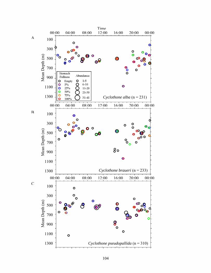
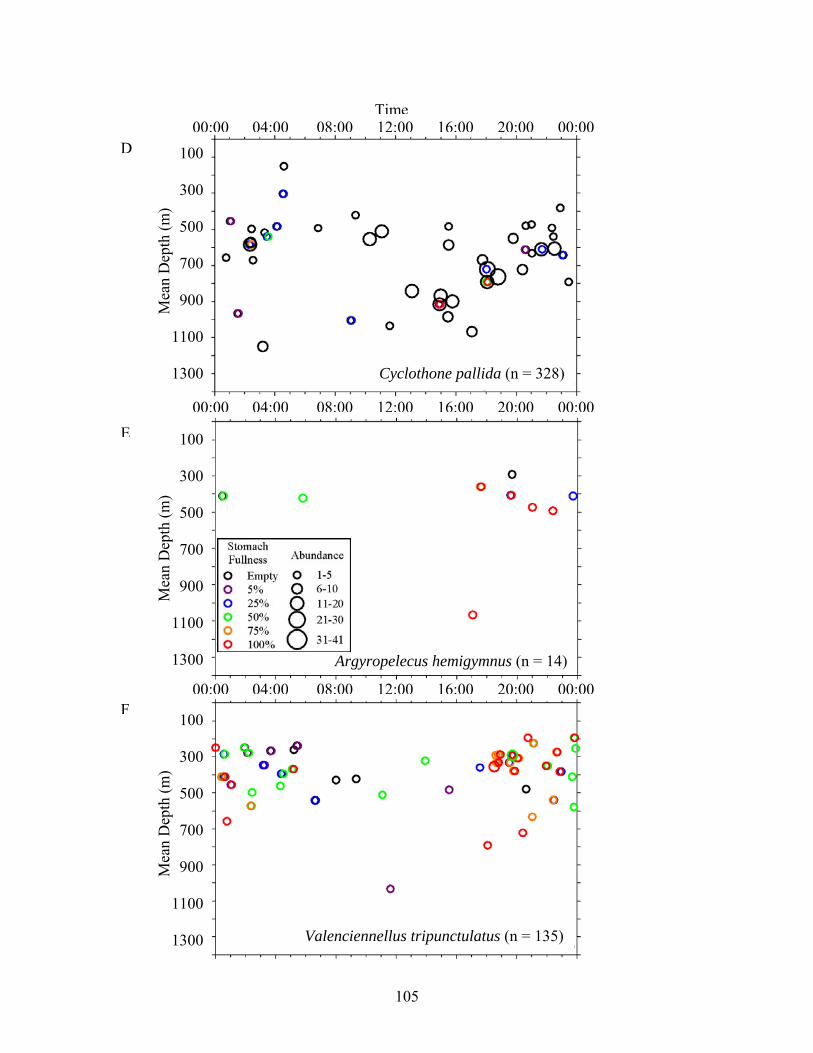
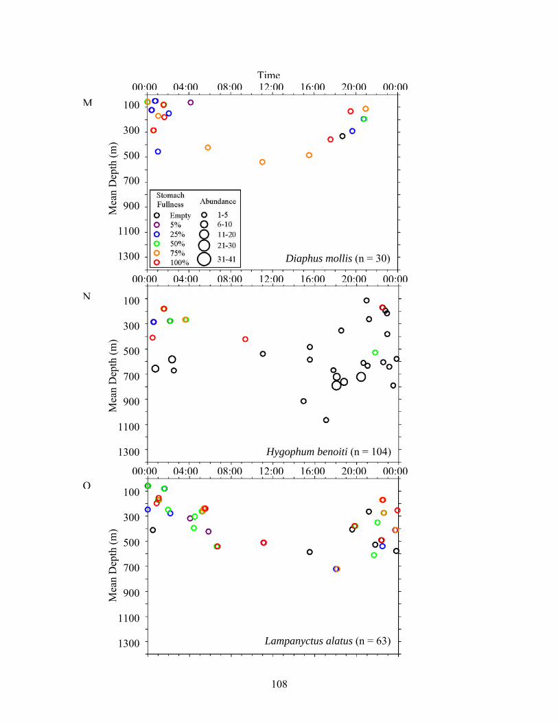
Figure 3. Relationships among stomach fullness, mean depth of capture and time for midwater fishes. Data were compiled from all sites and excluded specimens that lacked depth data. A) C. alba, B) C. braueri, C) C. pseudopallida, D) C. pallida, E) A. hemigymnus, F) V. tripunctulatus, G) G. elongatum, H) A. aculeatus, I) P. mauli, J) V. poweriae, K) B. suborbitale, L) C. warmingii, M) D. mollis, N) H. benoiti, O) L. alatus, P) L. guentheri, Q) N. valdiviae, R) M. affine, S) C. sloani, T) Stomiidae.

103

Time00:00 04:00 08:00 12:00 16:00 20:00 00:00

00:00 04:00 08:00 12:00 16:00 20:00 00:00

Cyclothone alba (n = 231)

100

300

500

700

900

1100

1300

100

300

500

700

900

1100

1300

100

300

500

700

900

1100

1300

Mea

n D

epth

(m)

Mea

n D

epth

(m)

Mea

n D

epth

(m)

Cyclothone braueri (n = 233)

Cyclothone pseudopallida (n = 310)

00:00 04:00 08:00 12:00 16:00 20:00 00:00

A

B

C

104

Time00:00 04:00 08:00 12:00 16:00 20:00 00:00

100

300

500

700

900

1100

1300

100

300

500

700

900

1100

1300

100

300

500

700

900

1100

1300

Mea

n D

epth

(m)

Mea

n D

epth

(m)

Mea

n D

epth

(m)

00:00 04:00 08:00 12:00 16:00 20:00 00:00

Argyropelecus hemigymnus (n = 14)

00:00 04:00 08:00 12:00 16:00 20:00 00:00

Cyclothone pallida (n = 328)

Valenciennellus tripunctulatus (n = 135)

D

E

F

105

Gonostoma elongatum (n = 78)

Time00:00 04:00 08:00 12:00 16:00 20:00 00:00

00:00 04:00 08:00 12:00 16:00 20:00 00:00

00:00 04:00 08:00 12:00 16:00 20:00 00:00

100

300

500

700

900

1100

1300

100

300

500

700

900

1100

1300

100

300

500

700

900

1100

1300

Mea

n D

epth

(m)

Mea

n D

epth

(m)

Mea

n D

epth

(m)

I

Pollichthys mauli (n = 58)

Argyropelecus aculeatus (n = 29)

H

G

106

Time00:00 04:00 08:00 12:00 16:00 20:00 00:00

00:00 04:00 08:00 12:00 16:00 20:00 00:00

100

300

500

700

900

1100

1300

100

300

500

700

900

1100

1300

100

300

500

700

900

1100

1300

Mea

n D

epth

(m)

Mea

n D

epth

(m)

Mea

n D

epth

(m)

J

K

L

Vinciguerria poweriae (n = 139)

00:00 04:00 08:00 12:00 16:00 20:00 00:00

Benthosema suborbitale (n = 193)

Ceratoscopelus warmingii (n = 75)

107

Hygophum benoiti (n = 104)

Diaphus mollis (n = 30)

Lampanyctus alatus (n = 63)

Time00:00 04:00 08:00 12:00 16:00 20:00 00:00

00:00 04:00 08:00 12:00 16:00 20:00 00:00

00:00 04:00 08:00 12:00 16:00 20:00 00:00

100

300

500

700

900

1100

1300

100

300

500

700

900

1100

1300

100

300

500

700

900

1100

1300

Mea

n D

epth

(m)

Mea

n D

epth

(m)

Mea

n D

epth

(m)

M

N

O

108

Time00:00 04:00 08:00 12:00 16:00 20:00 00:00

100

300

500

700

900

1100

1300

100

300

500

700

900

1100

1300

100

300

500

700

900

1100

1300

Lepidophanes guentheri (n = 127)

P

Q

R

Mea

n D

epth

(m)

Mea

n D

epth

(m)

Mea

n D

epth

(m)

Notolychnus valdiviae (n = 312)

00:00 04:00 08:00 12:00 16:00 20:00 00:00

Myctophum affine (n = 40)

00:00 04:00 08:00 12:00 16:00 20:00 00:00

109

110

Chauliodus sloani (n = 52)

Stomiidae (n = 26)

Time00:00 04:00 08:00 12:00 16:00 20:00 00:00

00:00 04:00 08:00 12:00 16:00 20:00 00:00

100

300

500

700

900

1100

1300

100

300

500

700

900

1100

1300

S

T

Mea

n D

epth

(m)

Mea

n D

epth

(m)

111

0

2

4

6

8

10

12

14

-22 -21 -20 -19 -18 -17

Cyclothone albaCyclothone pallidaCyclothone pseudopallidaGonostoma elongatumArgyropelecus aculeatusArgyropelecus hemigymnusValenciennellus tripunctulatusSternoptyx spp.Pollichthys mauliVinciguerria poweriaeChauliodus sloaniStomiidae (6 spp.)Benthosema suborbitaleCeratoscopelus warmingiiDiaphus problematicusDiaphus spp.Lampanyctus alatusLepidophanes guentheriMyctophum affineMelamphaidae (3 spp.)CavoliniidaeCephalopodaChaetgnathaCnidaria Salpidae Amphipoda Copepoda Euphausiacea Zooplankton Acanthephyra purpureaGennadas valensSystellaspis debilisPhytoplanktonSargassum spp.

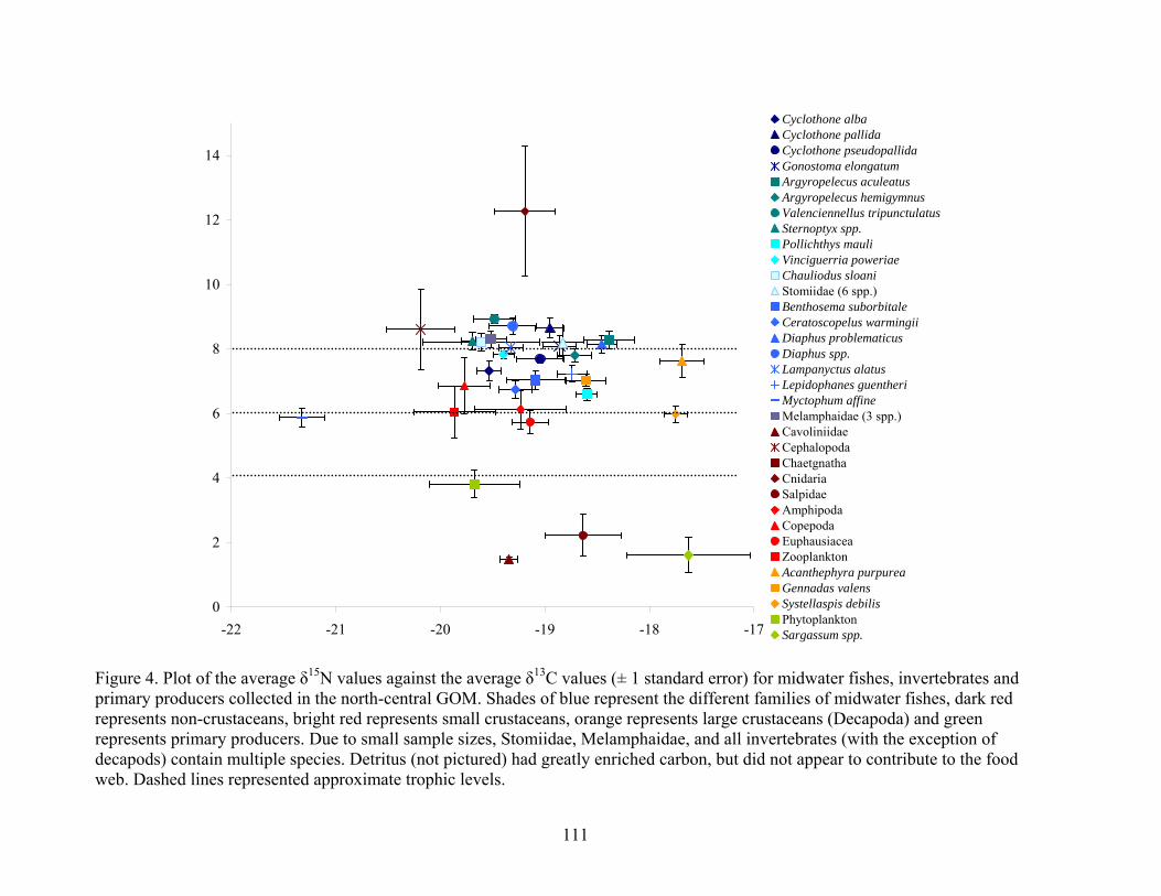
Figure 4. Plot of the average δ15N values against the average δ13C values (± 1 standard error) for midwater fishes, invertebrates and primary producers collected in the north-central GOM. Shades of blue represent the different families of midwater fishes, dark red represents non-crustaceans, bright red represents small crustaceans, orange represents large crustaceans (Decapoda) and green represents primary producers. Due to small sample sizes, Stomiidae, Melamphaidae, and all invertebrates (with the exception of decapods) contain multiple species. Detritus (not pictured) had greatly enriched carbon, but did not appear to contribute to the food web. Dashed lines represented approximate trophic levels.

A B

6.0

6.5

7.0

7.5

8.0

8.5

18 20 22 24 26 28 30 32 34 36

R2 = 0.223p = 0.646

R2 = 0.367p = 0.064

6.0

6.5

7.0

7.5

8.0

8.5

9.0

9.5

10.0

10.5

25 30 35 40 45 50

C D

R2 = 0.736p = 0.002

6.8

7.0

7.2

7.4

7.6

7.8

8.0

8.2

8.4

10 20 30 40 50

R2 = 0.618p = 0.002

6.0

6.5

7.0

7.5

8.0

8.5

9.0

9.5

10.0

0 50 100 150 200

E F

6.0

6.5

7.0

7.5

8.0

8.5

9.0

9.5

10.0

0 10 20 30 40 50 60

R2 = 0.400p = 0.068

6.0

6.5

7.0

7.5

8.0

8.5

9.0

0 10 20 30 40

R2 = 0.274p = 0.329

SL (mm)

δ15N

Figure 5. Relationship between δ15N and SL for midwater fish species. A) Cyclothone alba, B) Cyclothone pallida, C) Cyclothone pseudopallida, D) Gonostoma elongatum, E) Argyropelecus aculeatus, F) Argyropelecus hemigymnus, G) Sternoptyx spp., H) Valenciennellus tripunctulatus, I) Pollichthys mauli, J) Vinciguerria poweriae, K) Chauliodus sloani, L) Stomiidae, M) Benthosema suborbitale, N) Ceratoscopelus warmingii, O) Diaphus spp., P) Diaphus problematicus, Q) Lampanyctus alatus, R) Lepidophanes guentheri, S) Myctophum affine, T) Melamphaidae. The lines correspond to linear regressions.

112

G H

6.0

6.5

7.0

7.5

8.0

8.5

9.0

9.5

0 10 20 30 40 50 607.0

7.5

8.0

8.5

9.0

9.5

10.0

16 18 20 22 24 26 28

R2 = 0.123R2 = 0.509p = 0.399p = 0.128

I J

R2 = 0.331p = 0.082

5.0

5.5

6.0

6.5

7.0

7.5

8.0

24 29 34 39

R2 = 0.614p < 0.001

6.0

6.5

7.0

7.5

8.0

8.5

9.0

18 20 22 24 26 28 30 32

δ15N

K L

7.0

7.5

8.0

8.5

9.0

9.5

0 50 100 150 200 250

R2 = 0.852p = 0.009

R2 = 0.355p = 0.053

4.0

5.0

6.0

7.0

8.0

9.0

10.0

11.0

12.0

0 50 100 150 200 250 300 SL (mm)

Figure 5 cont. Relationship between δ15N and SL for all midwater fish species. A) Cyclothone alba, B) Cyclothone pallida, C) Cyclothone pseudopallida, D) Gonostoma elongatum, E) Argyropelecus aculeatus, F) Argyropelecus hemigymnus, G) Sternoptyx spp., H) Valenciennellus tripunctulatus, I) Pollichthys mauli, J) Vinciguerria poweriae, K) Chauliodus sloani, L) Stomiidae, M) Benthosema suborbitale, N) Ceratoscopelus warmingii, O) Diaphus spp., P) Diaphus problematicus, Q) Lampanyctus alatus, R) Lepidophanes guentheri, S) Myctophum affine, T) Melamphaidae. The lines correspond to linear regressions.

113

M N

6.0

6.5

7.0

7.5

8.0

18 19 20 21 22 23 24 25 26 27 28

R2 = 0.735p = 0.307

4.00

4.50

5.00

5.50

6.00

6.50

7.00

7.50

8.00

8.50

0 10 20 30 40 5

R2 = 0.356

0

p = 0.149

O P

R2 = 0.838p = 0.029

7.0

7.5

8.0

8.5

9.0

9.5

10.0

25 35 45 55 65 75

R2 = 0.738p = 0.013

7.0

7.5

8.0

8.5

9.0

9.5

40 45 50 55 60 65 70 75 80

δ15N

Q R

5.00

5.50

6.00

6.50

7.00

7.50

8.00

8.50

9.00

R2 = 0.113p = 0.220

6.0

6.5

7.0

7.5

8.0

8.5

9.0

9.5

25 30 35 40 45 50 55 35 40 45 50 55 60 65 70

R2 = 0.652p = 0.138

30 SL (mm) Figure 5 cont. Relationship between δ15N and SL for all midwater fish species. A) Cyclothone alba, B) Cyclothone pallida, C) Cyclothone pseudopallida, D) Gonostoma elongatum, E) Argyropelecus aculeatus, F) Argyropelecus hemigymnus, G) Sternoptyx spp., H) Valenciennellus tripunctulatus, I) Pollichthys mauli, J) Vinciguerria poweriae, K) Chauliodus sloani, L) Stomiidae, M) Benthosema suborbitale, N) Ceratoscopelus warmingii, O) Diaphus spp., P) Diaphus problematicus, Q) Lampanyctus alatus, R) Lepidophanes guentheri, S) Myctophum affine, T) Melamphaidae. The lines correspond to linear regressions.

114

S T

R2 = 0.408p = 0.047

4.0

4.5

5.0

5.5

6.0

6.5

7.0

7.5

13 14 15 16 17 18 19

R2 = 0.687p = 0.003

6.0

6.5

7.0

7.5

8.0

8.5

9.0

9.5

10.0

12 14 16 18 20 22 24 26 28

δ15N

SL (mm) Figure 5 cont. Relationship between δ15N and SL for all midwater fish species. A) Cyclothone alba, B) Cyclothone pallida, C) Cyclothone pseudopallida, D) Gonostoma elongatum, E) Argyropelecus aculeatus, F) Argyropelecus hemigymnus, G) Sternoptyx spp., H) Valenciennellus tripunctulatus, I) Pollichthys mauli, J) Vinciguerria poweriae, K) Chauliodus sloani, L) Stomiidae, M) Benthosema suborbitale, N) Ceratoscopelus warmingii, O) Diaphus spp., P) Diaphus problematicus, Q) Lampanyctus alatus, R) Lepidophanes guentheri, S) Myctophum affine, T) Melamphaidae. The lines correspond to linear regressions.

115

Date post:	03-Feb-2022
Category:	Documents
Upload:	others
View:	2 times
Download:	0 times

trophic structure of mesopelagic fishes over cold seeps in the north central gulf of mexico

Documents