Trygve Haavelmo and the Emergence of Causal Calculus

Trygve Haavelmo and the Emergence

of Causal Calculus

Judea PearlUniversity of California, Los Angeles

Computer Science DepartmentLos Angeles, CA, 90095-1596, USA

(310) [email protected]

Abstract

Haavelmo was the first to recognize the capacity of economic models to guide policies. Thispaper describes some of the barriers that Haavelmo’s ideas have had (and still have) to over-come, and lays out a logical framework that has evolved from Haavelmo’s insight and maturedinto a coherent and comprehensive account of the relationships between theory, data and policyquestions. The mathematical tools that emerge from this framework now enable investigatorsto answer complex policy and counterfactual questions using simple routines, some by mereinspection of the model’s structure. Several such problems are illustrated by examples, includ-ing misspecification tests, nonparametric identification, mediation analysis, and introspection.Finally, we observe that economists are largely unaware of the benefits that Haavelmo’s ideasbestow upon them and, to close this gap, we identify concrete recent advances in causal analysisthat economists can utilize in research and education.

1 Introduction

To students of causation, Haavelmo’s paper “The statistical implications of a system of simultaneousequations,” (Haavelmo, 1943) marks a pivotal turning point, not in the statistical implicationsof econometric models, as historians typically presume, but in their causal counterparts. Causalimplications, which prior to Haavelmo’s paper were cast to the mercy of speculation and intuitivejudgment have thus begun their quest for full membership in the good company of scientific discourse.

Haavelmo introduced three revolutionary insights in 1943.First, when an economist sits down to write a structural equation he/she envisions, not statistical

relationships but a set of hypothetical experiments, qualitative aspects of which are then encodedin the system of equations. Second, an economic model thus constructed is capable of answeringpolicy intervention questions, with no further assistance from the modeler. Finally, to demonstratethe feature above, Haavelmo presented a mathematical procedure that takes an arbitrary model andproduces quantitative answers to policy questions (see Section 1.3).

1.1 What is an economic model?

This first idea, that an economic model depicts a series of hypothetical experiments was expressedmore forcefully in Haavelmo’s 1944 paper (The Probability Approach in Econometrics) where hestates:

“What makes a piece of mathematical economics not only mathematics but also eco-nomics is, I believe, this: When we set up a system of theoretical relationships and useeconomic names for the otherwise purely theoretical variables involved, we have in mind

1

Econometric Theory, Special Issue on Haavelmo Centennial. Published online: 10 June 2014. DOI: http://dx.doi.org/10.1017/S0266466614000231

TECHNICAL REPORT R-391

June 2014

The Emergence of Causal Calculus 2

some actual experiment, or some design of an experiment, which we could at least imag-ine arranging, in order to measure those quantities in real economic life that we thinkmight obey the laws imposed on their theoretical namesakes.” (1944, p. 5)

But the methodological implications of this idea is demonstrated more explicitly in 1943, whereHaavelmo tries to explain what a modeller must have in mind in putting together two or moresimultaneous equations, say

y = ax+ ε1 (1)

x = by + ε2 (2)

Haavelmo first showed that, contrary to naive expectation, the term ax is not equal to E(Y |x)1

and, so, asked Haavelmo, what information did the modeller intend a to carry in Eq. (1), and whatinformation would a provide if we are able to estimate its value.

In posing this question, Haavelmo addressed the dilemma of incremental model construction.Given that the statistical content of a can only be discerned (if at all) by considering the entiresystem of equations, how can a modeller write down one equation at a time, without knowing whatthe meaning of the coefficients is in each equation. “What is then the significance of the theoreticalequations...” Haavelmo asked (1943, p. 11) and answered it immediately: “To see that, let usconsider, not a problem of passive predictions, but a problem of government planning.”

In modern terms, Haavelmo rejected the then-ruling paradigm that parameters are conveyors ofstatistical information and prepared the ground for the causal definition of a (Pearl, 1994):

a =∂

∂xE(Y |do(x)) (3)

which refers to a controlled experiment in which an agent (e.g., Government) is controlling x andobserving y.2 In such experiment, the average slope of Y on X (i.e., a) bears no relationship tothe regression slope (i.e., ∂

∂xE(Y |X = x)) in the population prior to intervention. Whereas thestatistical content of a (if identified) may come from many equations, its causal content is local – tothe great relief of most economists who think causally, not statistically.

This simple truth, which today is taken (almost) for granted, took a long time to take roots.To illustrate, the fierce debate between prominent statisticians and economists that flared up in1992, fifty years after Haavelmo’s paper, revolved precisely around this issue of interpreting themeaning of a. The economist in the debate, Arthur Goldberger (1992), claimed that ax in Eq. (1)may be interpreted as the expected value of Y “if x were fixed,” so that the a parameter “hasnatural meaning for the economist.” The statistician, Nanny Wermuth (1992), argued that, sinceax 6= E(Y |X = x), “the parameters in (1) cannot have the meaning Arthur Goldberger claimsthey have.” Summarizing their arguments, Wermuth concluded that structural coefficients havedubious meaning, and Goldberger retorted that statistics has dubious substance. Remarkably, eachside quoted Haavelmo to prove the other wrong, and both sides were in fact correct; structuralcoefficients have no meaning in terms of properties of joint distribution functions, the only meaningthat statisticians were willing to accept in the 1990’s. And statistics has no substance, if it excludesfrom its province all aspects of the data generating mechanism that do not show up in the jointdistribution, for example, a, or E(Y |do(x)).

The confusion did not end in 1992. The idea that an economic model must contain extra-statistical information, that is, information that can not be derived from joint densities, and thatthe gap between the two can never be bridged, seems to be very slow in penetrating the mind set

1Although Haavelmo used nonrecursive models to get his point across, this inequality prevails in almost all economicmodels, certainly those in which a is not identified.

2More precisely, the general definition of a is a = ∂∂x

[Yx,z(u)] where Yx,z(u) is the counterfactual “Y if x andz” for unit u (see Definition 1 and Appendix 1) and Z is any set of variables in the model (excluding X and Y ).However, counterfactuals were rather late to obtain a formal representation in structural economics (Balke and Pearl,1995; Heckman, 2000; Simon and Rescher, 1966). A simple recipe for computing E(Y |do(x)) from any given modelis given by Eq. (4) below, together with the identity P (Y = y|do(x)) = P (Yx = y). Note that it is only through thecausal interpretation of a that we can explain why an economist would exclude from Eq. (1) factors that are strongredactors of Y , yet are not deemed to be causes of Y .


of mainstream economists. Hendry, for example, wrote: “The joint density is the basis: SEMsare merely an interpretation of that” (Hendry, 1998, personal communication). Spanos (2010),expressing similar sentiments, hopes to “bridge the gap between theory and data” through theteachings of Fisher, Neyman and Pearson, disregarding the fact that the gap between data andtheory is fundamentally unbridgeable. This “data-first” school of economic research continues topursue such hopes, unable to internalize the hard fact that statistics, however refined, cannot providethe causal information that economic models must encode to be of use to policy making.3

The dominance of statistical thinking in econometrics goes beyond theory testing. A highly in-fluential econometric textbook writes: “A state implements tough new penalties on drunk drivers:What is the effect on highway fatalities?... [This effect] is an unknown characteristic of the popula-tion joint distribution of X and Y ” (Stock and Watson, 2011, Ch. 4, p. 107). The fact that “effects”are not characteristics of population joint distributions, so compellingly demonstrated by Haavelmo(1943; see Eq. (1)–(3)), would probably come as a surprise to modern authors of econometric texts.To witness, almost seventy years after Haavelmo defined a model as a set of hypothetical experi-ments, the common definition of “Econometric Models” reads (Wikipedia, February 18, 2012): “Aneconometric model specifies the statistical relationship that is believed to hold between the variouseconomic quantities pertaining to particular economic phenomena under study.”4

1.2 An oracle for policies or an aid to forecasters?

Haavelmo’s second and third insights also took time to be fully appreciated. Even today, the ideathat an economic model should serve as an oracle (i.e., a provider of valid answers to non-trivialquestions) for interventional questions tends to evoke immediate doubts and resistance: “How canone predict outcomes of experiments that were never performed, nor envisioned by the modeller?”Ask the skeptics. And if the modeller’s assumptions possess such clairvoyant powers, why not askthe modeller to answer policy questions directly, rather than engage in modeling and analysis? Howcan a set of ordinary equations encapsulate the information needed for predicting the vast varietyof interventions that a policy maker may wish to evaluate? How is this vast amount of informationencoded nonparametrically, and what means do we have to extract it from its encoding?5

To a large extent, this typical resistance stems from the absence of distinct mathematical notationfor marking the causal assumptions that enter into an economic model; the syntax of the equationsappears deceptively algebraic, similar to that of regression models, hence void of causal content.Some economists, lured by this surface similarity, were led to conclude: “We must first emphasizethat, disturbance terms being unobservable, the usual zero covariances “assumptions” generallyreduce to mere definitions and have no necessary causality and exogeneity implications.” (Richard,1980, p. 3).

The absence of distinct notation for causal assumptions further compelled economists to assumethat, to qualify for policy analysis, an economic model must be hardened by some extra ingredients;the equations themselves, even those ordained and causally interpreted by Haavelmo and the CowlesCommission, were deemed too simplistic or “fragile” to convey interventional information.

The literature on “exogeneity” (e.g. Engle, Hendry, and Richard, 1983; Hendry, 1995; Richard,1980) for example, sought such extra power in the notion of “parameter invariance.” Similarly,Cartwright (2007) views models as close to useless for policy evaluation because “the policy mayaffect a host of changes in other variables in the system, some envisaged and some not” (see Pearl

3Even the “faithfulness” assumption used in causal discovery algorithms (Pearl, 2000, Ch. 2; Pearl and Verma,1991; Spirtes, Glymour, and Scheines, 1993) is extra statistical, for it cannot be tested from density functions overobserved variables. This assumption, however, is milder than those made in structural equation modeling, for it isgeneric, and does not rely on problem-specific knowledge.

4I was tempted to correct this sentence in the Wikipedia, but decided to keep it as a witness to prevailing views, andas an incentive for editors of respected journals of econometrics to bring the issue to public discussion and collectiverevision.

5These rhetorical questions, which are rarely asked about physics or engineering, have repeatedly been posed tothe author about economic modeling, reflecting the general reluctance of economists to examine the power of non-parametric equations (as in Section 3.2). Another recurrent question goes: “How do we establish those assumptions?Don’t we sweep the most difficult issues under the rug when we agree to rely on them?” See footnote 11 and 12 forresponses.


2010d for rebuttal). And, in general, one would be hard pressed to find an economic textbook thatencourages readers to answer policy questions from the equations themselves, without resorting tometa-mathematical disclaimers or preconditions that reside outside the model.

This lack of confidence in the ability of economic models to guide policies has threatened theutility of the entire enterprise of economic modeling for, taken to extreme, it commits economicanalysis to statistical extrapolation of time series data. I doubt Haavelmo would agree to suchrestriction. Indeed, what is the point of parameter estimation if at the end of such exercise onemust appeal to judgment to decide which parameter is invariant and which is not, or, lacking suchjudgment, to physically trying out the policy and observing its effect on various parameters.

A more reasonable alternative, one that I have advocated in (Pearl, 2000) and that is gainingsupport among economists (e.g., Heckman, 2000, 2003, 2008; Keane, 2010; Leamer, 2010) is to treatan economic model as an oracle for all causally related queries, including questions of prospectiveand introspective counterfactuals and, simultaneously, insist on encoding the assumptions needed foranswering such queries within the model itself, not external to it. In other words, these assumptionsshould be guiding the modeller in the way the equations are authored. Moreover, even if the modelis misspecified it can still be useful to policy makers, if each of its conclusion is accompanied bya meaningful set of assumptions, as long as as each assumption points to a condition that couldconceivably be realizable or achievable.

“And what if an intervention changes the very equation that purports to predict its effect?” askthe critics and cite Lucas Jr. (1976), who attributed the predictive failure of macro-econometricmodels of the 1960s and 1970s to their non-invariance under changes of policy regime. What Lucasargued in fact was that, to get useful policy advice from a model we have to a) specify the modelcorrectly and b) pose the right questions to it. Since the model provides the facility for encodingside effects associated with any given implementation of the policy evaluated, neglecting to encodethem in the model constitutes a case of query misspecification, posing no lesser threats than modelmisspecification. In other words, if an intervention I, intended to increase variable X from X = xto X = x′, has a side effect on some other variables or parameters, it would be inappropriate toseek the estimation of P (y|do(x′)); the proper query should be the estimation of P (y|do(I)), so asto take into account the various side effects of I.6 The burden of properly specifying queries restswith the query provider not with the model.

1.3 The algorithmization of interventions

Modern days interest in causal models and their tentative conclusions, owes its renaissance toHaavelmo’s third insight – a concrete procedure for eliciting answers to policy questions from themodel equations. This he devised at the end of his 1943 paper:

“Assume that the Government decides, through public spending, taxation, etc., to keepincome, rt, at a given level, and that consumption ui and private investment vi continueto be given by (2.5) and (2.6), the only change in the system being that, instead of (2.7),we now have

ri = ui + vi + gi (2.7′)

where gi is Government expenditure, so adjusted as to keep r constant, whatever be uand v,...” (1943, p. 12)

This idea of simulating an intervention on a variable by modifying the equation that determinesthat variable while keeping all other equations intact is the basis of all currently used formalismsof causal inference. Haavelmo’s proposal of adding an adjustable term to the equation so as tokeep the manipulated variable constant differs somewhat from Fisher’s proposal of subjecting such avariable to randomized external variations. Haavelmo was more interested in simulating the actual

6Cartwright’s 2007 used the term “impostor counterfactuals” to describe the consequences of substituting com-pound interventions (e.g., do(I)) with atomic interventions (e.g., do(x)) (see (Hoover, 2011; Pearl, 2010d)). Compoundinterventions are analyzed by computing the simultaneous effects of their atomic components (Pearl, 2000, Ch. 4),which may consist of mild or drastic changes in the equations themselves (Pearl, 2000, Section 3.2.3).


implementation of a pending policy, rather than the Fisherian experiment from which we may learnabout the average effect of the policy.

Haavelmo’s approach was later transformed by Strotz and Wold (1960) into the operation of“wiping out” the equation altogether, and was further translated into graphical models as “wipingout” incoming arrows into the manipulated variable (Pearl, 1993; Spirtes et al., 1993).7 This opera-tion, called do-operator, has subsequently led to do-calculus (Pearl, 1994, 2000) and to the structuraltheory of counterfactuals (Balke and Pearl, 1995; Pearl, 2000, Ch. 7), which unifies structural equa-tion modeling with the potential outcome paradigm of Neyman (1923) and Rubin (1974) and thepossible-world semantics of Lewis (1973).

Key to this unifying framework has been a symbolic procedure for reading counterfactual infor-mation in a system of economic equations, as articulated in the following Definition:

Definition 1 (unit-level counterfactuals) (Pearl, 2000, p. 98)Let M be a fully specified structural model and X and Y two arbitrary sets of variables in M . LetMx be a modified version of M , with the equation(s) of X replaced by X = x (see Fig. 2(b), Section3.1). Denote the solution for Y in the modified model by the symbol YMx(u), where u stands for thevalues that the exogenous variables take for any given individual (or unit) in the population. Thecounterfactual Yx(u) (Read: “The value of Y in unit u, had X been x”) is defined by

Yx(u)∆= YMx(u). (4)

In words: The counterfactual Yx(u) in model M is defined by the solution for Y in the modifiedsubmodel Mx, with the exogenous variables held at U = u. For example, in Haavelmo’s model ofequations (1)–(2), the modified model Mx(u) consists of Eq. (1) alone, with x treated as a constant.The counterfactual Yx(u) therefore becomes ax+ ε1(u), with ε1(u) standing for the omitted factorsthat characterize unit U = u.8

We see that every structural equation, say y = ax + ε1(u) (Eq. (1)), carries counterfactualinformation, Yx(u) = ax+ε1(u), which, in our simple case, conveys the assumptions of effect-linearityand effect homogeneity (i.e., Yx(u) − Yx′(u) = a(x − x′), for all u). The structural assumption isin fact much stronger. The fact that the equation contains only X on the right hand side conveysthe counterfactual assumption (known as an “exclusion restriction”) Yxz(u) = ax+ ε1(u), where Zis any set of variables (in the model) that does not appear on the right hand side of the equation.The exclusion restriction and linearity assumption are refutable in interventional experiments, notso the homogeneity assumption.9 Naturally, when the exogenous variables U in a model are randomvariables, the counterfactual Yx will be a random variable as well, the distribution of which is dictatedby both the distribution P (U = u) of the exogenous variables and the structure of the model Mx.This interpretation permits us to define joint distributions of counterfactual variables and to detectconditional independencies of counterfactuals directly from the structure of the model (Pearl, 2000,Ch. 7).

Equation (4) constitutes the bridge between the structural interpretation of counterfactuals andthe potential outcome framework advanced by Neyman (1923) and Rubin (1974), which takes thecontrolled randomized experiment as its guiding paradigm (see Appendix 1). One of the maindifferences between the two frameworks is that counterfactuals, as well as assumptions such as “ig-norability,” “sequential ignorability,” or “instrumentality” can actually be derived from the economicmodel (see Appendix 1); they need not be imposed as separate assumptions external to, and obliv-ious to the model. Another difference is that the antecedent x in the structural interpretation of

7Figure 2(b) (Sectioin 3.1) provides a graphical representation of the model that results from Haavelmo’s inter-vention. Some authors prefer to retain those arrows in the graph and split outgoing arrows instead (Heckman andPinto, 2013); the resulting equations and all their implications are the same (Pearl, 2013b).

8The set of units characterized by the same values U = u of the exogenous variables form an equivalent class. Wetherefore do not distinguish between “unit” as an index for individual identity and “unit” as a specific instantiationU = u of the exogenous variables.

9Anecdotically, none of the six textbooks surveyed in (Chen and Pearl, 2013) explains to readers what justifi-cation there is for excluding variables from an equation; such explanations require that equations be given causalinterpretation, which textbooks are reluctant to do.


Yx(u) need not be a manipulable treatment but may consist of any exogenous or endogenous vari-able (e.g., sex, genetic traits, race, earning) that affects Y as part of a social or biological process(Heckman, 2008). This interpretation has extended Haavelmo’s theory of interventions from linearto nonparametric analysis and permitted questions of identification, estimation, and generalizationto be handled with mathematical precision and algorithmic simplicity (see Section 3).

Haavelmo did not deem his intervention theory to be revolutionary, but natural. In his words:

“That is, to predict consumption ... under the Government policy,... we may use the‘theoretical’ equations obtained by omitting the error terms...”“this is only natural, because now the Government is, in fact, performing ‘experiments’of the type we had in mind when constructing each of the two equations.” (1943, p. 12)

I do consider it revolutionary in that it defines the effect of interventions not in terms of themodel’s parameters but in terms of a procedure (or “surgery”) that hypothetically modifies thestructure of the model so as to simulate the actual intervention.10 It thus liberates economic analysisfrom its dependence on parametric representations and permits a totally nonparametric calculus ofcauses and counterfactuals that makes the connection between assumptions and conclusions explicitand transparent.

In the next section I will give a brief summary of nonparametric structural models and the wealthof mathematical tools that they now offer to economists and other policy-minded data analysts.

2 The Logic of Structural Causal Models (SCM)

This section describes a coherent theory of causal inference that I propose to call Structural CausalModel (SCM). It takes seriously the original insights of Haavelmo and the subsequent philosophyof the Cowles Commission program and, enriched with a few ideas from logic and graph theory,provides a unifying framework for all known approaches to causation.

A simple way to view SCM is to imagine a logical machine, or an inference engine,11 that takesthree inputs and produces three outputs. The inputs are:

I-1. A set A of qualitative causal assumptions that the investigator is prepared to defend on scientificgrounds, and a model MA that encodes these assumptions. Traditionally, MA takes the formof a set of structural equations with undetermined parameters. A typical assumption is thatcertain omitted factors, represented by error terms, are uncorrelated, or that no direct effectexists between a pair of variables (i.e., an “exclusion restriction”).

I-2. A set Q of queries concerning causal and counterfactual relationships among variables of in-terest. Traditionally, Q concerned the magnitudes of structural parameters but, in general, Qmay address causal relations more directly, e.g.,

Q1 : What is the effect of treatment X on outcome Y ?

Q2 : Is this employer guilty of gender discrimination?

Formally, each query Qi ∈ Q should be computable from a fully specified theoretical modelM in which all functional relationships are given, together with the joint distribution of allomitted factors. Non-computable queries are inadmissible.

10Fearing violation of modularity, Cartwright (2007) and Heckman and Vytlacil (2007) voiced objections to hypo-thetical modifications of the model’s equations as proposed by Haavelmo. These objections are addressed in (Pearl,2009a, pp. 362–265, 374–380), with emphasis on the fundamental distinctions between definition, identification, es-timation, and implementation, which become crisp and unambiguous in nonparametric structural causal models(Section 2).

11These terms are chosen to emphasize that, in dealing with econometric modeling, it is essential to separate thelogic of the method from the veracity of its premises. Surely, the long term goal of economics is to see every premisesubstantiated by compelling empirical evidence, and the importance of efforts to establish such evidence from sourcesresiding outside the model is far from being overlooked by this author. However, in any given study, including thoseevidence-seeking efforts, the aim is to take what little theoretical knowledge we have, and make sure it is maximallyutilized, while acknowledging its provisional status.


I-3. A set D of experimental or non-experimental data.

The outputs are

O-1. A set A∗ of statements which are the logical implications of A, prior to obtaining any data.For example, that X has no effect on Y if we hold Z constant, or that Z is an instrumentrelative to a pair {X, Y }.

O-2. A set C of data-dependent claims (or conclusions) concerning the magnitudes or likelihoodsof the target queries in Q, each conditional of A. C may contain, in the simple case, theestimated mean and variance of a given structural parameter, or the expected effect of a givenintervention or, to illustrate a counterfactual query, the probability that a student trained ina given program who now earns 50K per year would not have reached a salary level gre aterthan 30K had he/she not been trained (Pearl, 2000, Ch. 9).

Auxiliary to C, SCM also generates an estimand Qi(P ) for each query in Q, or a determinationthat Qi is not identifiable from P , the joint density of observed variables.

O-3. A list T of testable statistical implications of A, and the degree g(Ti), Ti ∈ T , to which thedata agrees with each of those implications. A typical implication would be the vanishing of aspecific regression coefficient, or the invariance of such coefficient to the addition or removal of agiven regressor; such constraints can be read from the model MA and confirmed quantitativelyby the data.

The structure of this inferential exercise is shown schematically in Fig. 1.

Q D, A( )Q − QEstimates of ( )P

M( )A

g T( )

Data( )D

( ) −Q P T MA( ) −

CAUSALA − ASSUMPTIONS

LogicalA* − implications of A

CConditional claims ( )

Statistical inference

Model testing

Causal inference

CAUSALMODEL

Goodness of fit

Identified estimands Testable implications

Queries of interestQ −

−I 1 −O 1

−O 3−O 2

−O 3−O 2

−I 3

−I 2

Figure 1: SCM methodology depicted as the an inference engine converting assumptions (A), queries(Q), and data (D) into logical implications (A∗) Conditional claims (C) and data-fitness indices(g(T )).

Several observations are worth noting before illustrating these inferences by examples. First, SCMis not a traditional statistical methodology, typified by hypothesis testing or estimation, becauseneither claims nor assumptions are expressed in terms of probability functions of realizable variables(Pearl, 2000).

Second, all claims produced by SCM are conditional on the validity of A, and should be reportedin conditional format: “If A then Ci” for any claim Ci ∈ C. Such claims assert that anyone willingto accept A, must also accept Ci out of logical necessity. Moreover, no other method can do better,


that is, if SCM analysis finds that a subset A′ of assumptions is necessary for inferring a claim Ci,no other methodology can infer Ci with a weaker set of assumptions. This follows from castingthe relationship between A and C in a formal mathematical system, coupled with the completenesstheorems of Halpern (1998) and Shpitser and Pearl (2008).12

Thirdly, passing a goodness-of-fit test is not a prerequisite for the validity of the conditional claim“If A then Ci,” nor for the validity of Ci. While it is important to know if any assumptions in A areinconsistent with the data, MA may not have any testable implications whatsoever. In such a case(traditionally called “just identified”), the assertion “If A then Ci” may still be extremely informativein a decision making context, since each Ci conveys quantitative information extracted from the datacompared with the qualitative assumptions A with which the study commences. Moreover, even ifA turns out inconsistent with D, the inconsistencies may be entirely due to portions of the modelwhich have nothing to do with the derivation of Ci (Marschak, 1953). It is therefore important toidentify which statistical implication of A is responsible for the inconsistency; while global tests forgoodness-of-fit hide this information, a variety of local tests have been developed as more viablealternatives (Pearl 2000, pp. 144-45; 2004).

Finally, and this has been realized by many researchers in the 1980’s, there is nothing in SCM’smethodology to protect C from the inevitability of contradictory equivalent models, namely, modelsthat satisfy all the testable implications of MA and still advertise claims that contradict C (seefootnote 19). Modern developments in graphical modeling have devised visual and algorithmic toolsfor detecting, displaying, and enumerating these equivalent models (Kyono, 2010). Researchersshould keep in mind therefore that only a tiny portion of the assumptions behind each SCM lendsitself to scrutiny by the data; the bulk of it must remain untestable, substantiated by scientifictheories, controlled experiments, or conclusions of causal discovery algorithms (Pearl, 2000, Ch. 2;Pearl and Verma, 1991; Spirtes et al., 1993).

It is also important to emphasize that the inferential tools provided by SCM cannot be replacedor evaded by appealing to so called “alternative approaches” to causation, or to “causal pluralism”(Cartwright, 2007). The abilities (1) to articulate assumptions formally and transparently, (2) todecide if they permit identification and (3) to detect whether they have testable implications arethree inescapable components of any “approach” that claims to guide policy.13

3 Causal Calculus, Tools, and Frills

By “causal calculus” I mean mathematical machinery for performing the computational tasks de-scribed in the inference engine of Fig. 1.

These include:

1. Tools of reading and explicating the causal assumptions embodied in structural models as wellas the set of assumptions that support each individual causal claim.

2. Methods of identifying the testable implications (if any) of the assumptions encoded in themodel, and ways of testing, not the model in its entirety, but the testable implications of theassumptions behind each causal claim.

3. Methods of deciding, prior to taking any data, what measurements ought to be taken, whetherone set of measurements is as good as to another, and which adjustments need to be made soas to render our estimates of the target quantities unbiased.

12This is important to emphasize in view of often heard critics that, in SCM, one must start with a model in whichall causal relations are presumed known, at least qualitatively. This is not so. It is common to start with a modelin which no causal relation is assumed known, and ask “what must be ascertained in order to answer the researchquestion at hand?” Additionally, if some causal assumptions in the model are found necessary, no other methodcan get away with weaker assumptions, though some tend to hide the assumptions under catch-all terms such as“ignorability,” “as if randomized,” “exchangeability,” “quasi-experiment,” “exogeneity,” and the like.

13Remarkably, none of these components is currently taught in econometric classes (Chen and Pearl, 2013), andnone is known to mainstream econometric researchers.


4. Methods for devising critical statistical tests by which two competing theories can be distin-guished.

5. Methods of deciding mathematically if the causal relationships of interest are estimable fromnon-experimental data and, if not, what additional assumptions, measurements or experimentswould render them estimable.

6. Methods of recognizing and generating equivalent models.

7. Methods of locating instrumental variables for any relationship in a model, or turning variablesinto instruments when none exists (Brito and Pearl, 2002).

8. Methods of evaluating “causes of effects” and predicting effects of choices that differ from theones actually made, as well as the effects of dynamic policies which respond to time-varyingobservations.

9. A solution to the so-called “Mediation Problem,” which estimates the degree to which specificmechanisms contribute to the transmission of a given effect, in models containing both con-tinuous and categorical variables, linear as well as nonlinear interactions (Pearl, 2001, 2012b).

10. A principled treatment of the problem of “external validity” (Campbell and Stanley, 1963),including, formal methods of deciding if a causal relation estimated in one population can betransported to another population, in which experimental conditions are different (Pearl andBareinboim, 2011).

A full description of these techniques is given in (Pearl, 2000) as well as in recent survey papers(Pearl, 2010a,b). Here I will demonstrate by examples how some of the simple tasks listed aboveare handled in the nonparametric framework of a SCM.

3.1 Two models for discussion

Consider a nonparametric structural model defined over a set of endogenous variables {Y,X,Z1,Z2, Z3,W1,W2,W3}, and unobserved exogenous variables {U,U ′, U1, U2, U3, U

′1, U

′2, U

′2, U

′3}. The

equations are assumed to be structured as follows:

Model 1

Y = f(W3, Z3,W2, U) X = g(W1, Z3, U′)

W3 = g3(X,U ′3) W1 = g1(Z1, U′1)

Z3 = f3(Z1, Z2, U3) Z1 = f1(U1)W2 = g2(Z2, U

′2) Z2 = f2(U2)

f, g, f1, f2, f3, g1, g2, g3 are arbitrary, unknown functions, and all exogenous variables are mutuallyindependent but otherwise arbitrarily distributed.

For the purpose of our illustration, we will avoid assigning any economic meaning to the vari-ables and functions involved, thus focusing on the formal aspects of such models rather than theirsubstance. The model conveys two types of theoretical (or causal) assumptions:

1. Exclusion restrictions, depicted by the absence of certain variables from the arguments ofcertain functions, and

2. Causal Markov conditions, depicted by the absence of common U -terms in any two functions,and the assumption of mutual independence among the U ′s.

Given the qualitative nature of these assumptions, the algebraic representation is superfluous andcan be replaced, without loss of information, with the diagram depicted in Fig. 2(a).14 To anchorthe discussion in familiar grounds, we also present the linear version of Model 1:

14This is entirely optional; readers comfortable with algebraic representations are invited to stay in their comfortzone.


(b)(a)

Z1Z2

W2

W3

W1

Z3

Y

X

Z1Z2

W2

W3

W1

Z3

Y

X = x

Figure 2: (a) A graphical representation of Model 1. Error terms are assumed mutually independentand not shown explicitly. (b) A graphical representation of Haavelmo’s hypothetical model Mx

under the policy do(X = x).

Model 2 (Linear version of Model 1)

Y = aW3 + bZ3 + cW2 + U X = t1W1 + t2Z3 + U ′

W3 = c3X + U ′3 W1 = a′1Z1 + U ′1Z3 = a3Z1 + b3Z2 + U3 Z1 = U1

W2 = c2Z2 + U ′2 Z2 = U2

All U ′s are assumed to be uncorrelated.

In our case, the recursive nature of the equations of Model 1 results in a Directed Acyclic Graph(DAG), a structure that will be assumed throughout this paper. The basic principles of Havvelmo’sintervention (e.g., Definition 1) are also applicable to systems with simultaneous equations (reciprocalcausation), represented to cyclic graphs, though some of the computational tasks become moreinvolved. While the orthogonality assumption renders these equations regressional, we can easilyillustrate non-regressional models by assuming that some of the variables are not measurable.

3.2 Illustrating typical question-answering tasks

Given the model defined above, the following are typical questions that an economist may wish toask.

3.2.1 Testable implications (misspecification tests)

a. What are the testable implications of the assumptions embedded in Model 1?

b. Assume that only variables X,Y, Z3, and W3 are measured, are there any testable implications?

c. The same, but assuming only variables X,Y , and Z3 are measured,

d. The same, assuming all but Z3 are measured.

e. Assume that an alternative model, competing with Model 1, has the same structure, with theZ3 → X arrow reversed. What statistical test would distinguish between the two models?

f. What regression coefficient in Model 2 would reflect the test devised in (e)?

3.2.2 Equivalent models

a. Which arrows in Fig. 2(a) can be reversed without being detected by any statistical test?

b. Is there an equivalent model (statistically indistinguishable) in which Z3 is a mediator betweenX and Y (i.e., the arrow X ← Z3 is reversed)?


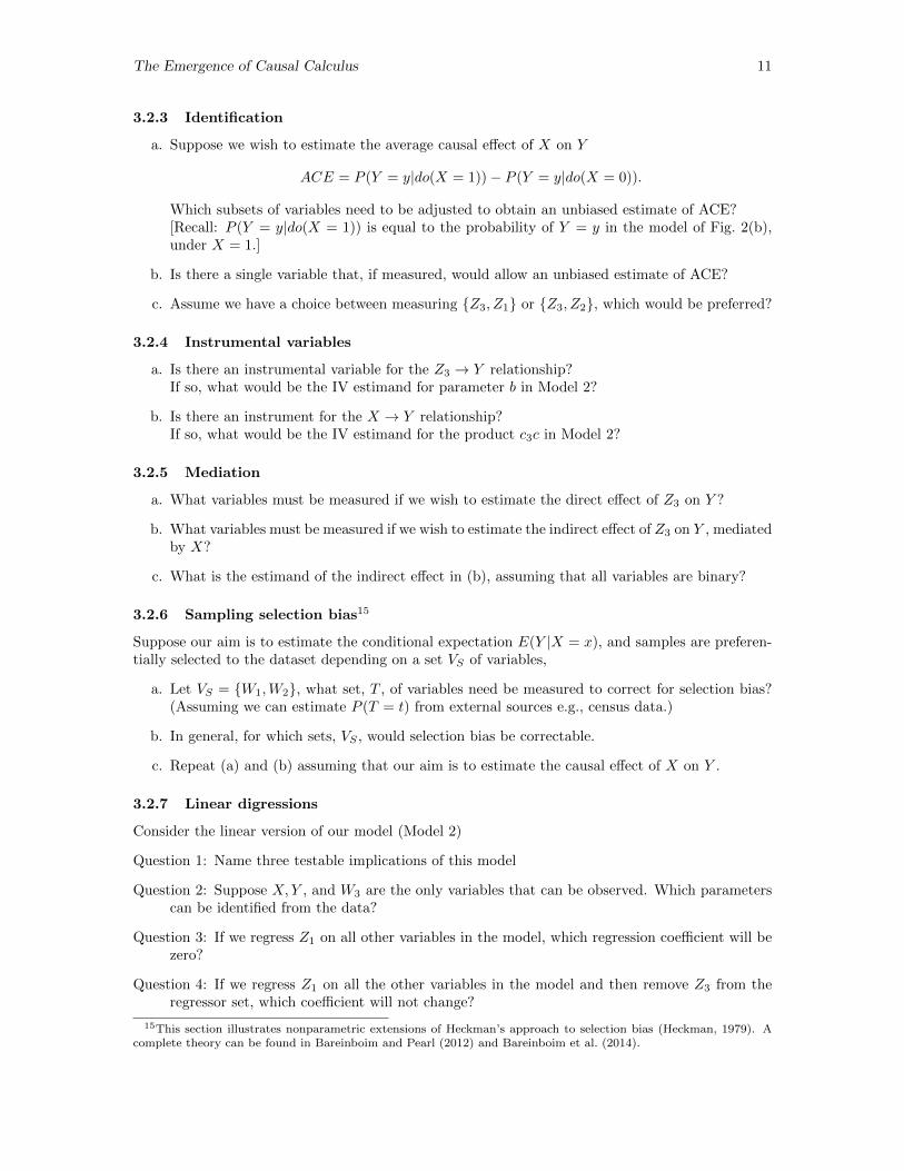
3.2.3 Identification

a. Suppose we wish to estimate the average causal effect of X on Y

ACE = P (Y = y|do(X = 1))− P (Y = y|do(X = 0)).

Which subsets of variables need to be adjusted to obtain an unbiased estimate of ACE?[Recall: P (Y = y|do(X = 1)) is equal to the probability of Y = y in the model of Fig. 2(b),under X = 1.]

b. Is there a single variable that, if measured, would allow an unbiased estimate of ACE?

c. Assume we have a choice between measuring {Z3, Z1} or {Z3, Z2}, which would be preferred?

3.2.4 Instrumental variables

a. Is there an instrumental variable for the Z3 → Y relationship?If so, what would be the IV estimand for parameter b in Model 2?

b. Is there an instrument for the X → Y relationship?If so, what would be the IV estimand for the product c3c in Model 2?

3.2.5 Mediation

a. What variables must be measured if we wish to estimate the direct effect of Z3 on Y ?

b. What variables must be measured if we wish to estimate the indirect effect of Z3 on Y , mediatedby X?

c. What is the estimand of the indirect effect in (b), assuming that all variables are binary?

3.2.6 Sampling selection bias15

Suppose our aim is to estimate the conditional expectation E(Y |X = x), and samples are preferen-tially selected to the dataset depending on a set VS of variables,

a. Let VS = {W1,W2}, what set, T , of variables need be measured to correct for selection bias?(Assuming we can estimate P (T = t) from external sources e.g., census data.)

b. In general, for which sets, VS , would selection bias be correctable.

c. Repeat (a) and (b) assuming that our aim is to estimate the causal effect of X on Y .

3.2.7 Linear digressions

Consider the linear version of our model (Model 2)

Question 1: Name three testable implications of this model

Question 2: Suppose X,Y , and W3 are the only variables that can be observed. Which parameterscan be identified from the data?

Question 3: If we regress Z1 on all other variables in the model, which regression coefficient will bezero?

Question 4: If we regress Z1 on all the other variables in the model and then remove Z3 from theregressor set, which coefficient will not change?

15This section illustrates nonparametric extensions of Heckman’s approach to selection bias (Heckman, 1979). Acomplete theory can be found in Bareinboim and Pearl (2012) and Bareinboim et al. (2014).


Question 5: (“Robustness” – a more general version of Question 4.) Model 2 implies that certainregression coefficients will remain invariant when an additional variable is added as a regressor.Identify five such coefficients with their added regressors.16

3.2.8 Counterfactual reasoning

a. Find a set S of endogenous variables such that X would be independent of the counterfactualYx conditioned on S.

b. Determine if X is independent of the counterfactual Yx conditioned on all the other endogenousvariables.

c. Determine if X is independent of the counterfactual W3,x conditioned on all the other endoge-nous variables.

d. Determine if the counterfactual relationship P (Yx|X = x′) is identifiable, assuming that onlyX,Y , and W3 are observed.

3.3 Solutions

The problems posed in Section 3.2 read like homework problems in Economics 101 class. Theyshould be! Because they are fundamental, easily solvable, and absolutely necessary for even themost elementary exercises in nonparametric analysis. Readers should be pleased to know that withthe graphical techniques available today, these questions can generally be answered by a quick glanceat the graph of Fig. 2 (see, for example, Greenland and Pearl (2011), Kyono (2010), or Pearl (2010a,b,2012a)).

More elaborate problems, like those involving transportability or counterfactual queries mayrequire the inferential machinery of do-calculus or counterfactual logic. Still, such problems havebeen mathematized, and are no longer at the mercy of unaided intuition, as they are presented forexample in Campbell and Stanley (1963).

It should also be noted that, with the exception of our linear digression (3.2.7) into Model 2, allqueries were addressed to a purely nonparametric model and, despite the fact that the form of ourequations and the distribution of the U ’s are totally arbitrary, we were able to extract answers topolicy-relevant questions in a form that is estimable from the data available.

For example, the answer to the first identification question (a) is: The set {W1, Z3} is sufficientfor adjustment and the resulting estimand is:

P (Y = y|do(X = x)) =∑w1,z3

P (Y = y|X = x, Z3 = z3,W1 = w1)P (Z3 = z3,W1 = w1).

This can be derived algebraically using the rules of do-calculus or seen directly from the graph,using the back-door criterion (Pearl, 1993), which has become an indispensable tool for confoundingcontrol in epidemiology (Glymour and Greenland, 2008; Vansteelandt and Lange, 2012) and socialscience (Morgan and Winship, 2007). When a policy question is not identifiable, graphical methodscan detect it and exit with failure. Put in econometric vocabulary, these results mean that theidentification problem in nonparametric triangular simultaneous equations models is now solved.Given any such model, an effective algorithm exists that decides if the causal effect of any subset ofvariables on another is identifiable and, if so, the algorithm delivers the correct estimand (Shpitserand Pearl, 2008).

16According to White and Lu (2014) “A common exercise in empirical studies is a ‘robustness check,’ where theresearcher examines how certain ‘core’ regression coefficient estimates behave when the regression specification ismodified by adding or removing regressors.” “of the 98 papers published in The American Economic Review during2009, 76 involve some data analysis. Of these, 23 perform a robustness check along the lines just described, usinga variety of estimators.” Oster (2013) finds that 75% of 2012 papers published in The American Economic Review,Journal of Political Economy, and Quarterly Journal of Economics sensitivity to added regressors as indicative ofmisspecification. Since this practice is conducted to help diagnose misspecification, the answer to Question 5 isessential for discerning whether an altered coefficient indicates misspecification or not.


The nonparametric nature of these exercises represents the ultimate realization of what Heckmancalls the Marschak’s Maxim (Heckman, 2010), referring to an observation made by Jacob Marschak(1953) that many policy questions do not require the estimation of each and every parameter inthe system – a combination of parameters is all that is necessary and, moreover, it is often possibleto identify the desired combination without identifying the individual components. The exercisespresented above show that Marschak Maxim goes even further – the desired quantity can often beidentified without ever specifying the functional or distributional forms of these economic models.

This nonparametric generality does not mean of course that graphical methods cannot accom-modate stronger assumptions on the functions in the model, such as linearity, homogeneity, mono-tonicity or separability. For example, DAGs have provided critical insights into the behavior oflinear causal systems (Pearl, 2013a). The most powerful identification results in linear econometricmodels have recently been derived using DAGs (Brito and Pearl, 2002; Foygel, Draisma, and Driton,2012). The use of instrumental variables, which some authors refer to as “The Roy model” (Heck-man and Pinto, 2013) has been extended substantially in both acyclic (Brito and Pearl, 2006) andcyclic (Phiromswad and Hoover, 2013) models. The instrumental inequality (Pearl, 2009a, p. 279)and tight bounds on the binary Roy Model (Balke and Pearl, 1997) were derived through DAG’srepresentations. Finally, mediation and moderation effects in nonlinear parametric systems (Pearl,2014) and attribution problems in monotonic systems (Pearl, 2009a, Ch. 9) are examples of specificidentification constraints incorporated within the graphical model framework.

3.4 What kept the Cowles Commission at bay?

A natural question to ask is why these recent developments have escaped the attention of Marschakand the Cowles Commission who, around 1950, already adopted Haavelmo interpretation of struc-tural models, and have formulated mathematically many of the key concepts and underlying theoriesthat render structural models useful for policy making, including theories of identification, structuralinvariance and structural estimation. What then prevented them from making the next logical moveand tackle nonparametric models such as those exemplified in Section 3.2?

I believe the answer lies in two ingredients that where not available to Cowles Commission’sresearchers and which are necessary for solving nonparametric problems. (These had to wait for the1980–90’s to be developed.) I will summarize these ingredients as “principles” since the entire setof tools needed for solving these problems emanate from these two:

Principle 1: “The law of structural counterfactuals.”

Principle 2: “The law of structural independence.”

The first principle is described in Definition 1 and instructs us how to compute counterfactualsfrom an economic model M . Simon and Rescher (1966) came close to this definition but, lackingthe “wiping out” operator, could not reconcile the contradiction that evolves when an observationX = x′ clashes with the antecedent X = x of the counterfactual Yx. Later economists, like Roy andQuandt, although they used counterfactual reasoning in their writings (Heckman, 2008), lacked thesyntactic machinery for reading counterfactuals from a model, and could not therefore develop thetools necessary for solving the problems presented in Sections 3.2.3, 3.2.5, and 3.2.8.

Principle 2 instructs us how to detect conditional independencies from the structure of themodel, i.e., the graph. This principle states that, regardless of the functional form of the equationsin a recursive model M , and regardless of the distribution of the exogenous variables U , if thedisturbances are mutually independent, the distribution P (v) of the endogenous variables mustobey certain conditional independence relations, stated roughly as follows:

Whenever sets X and Y of nodes in the graph are “separated” by a set Z, X is indepen-dent of Y given Z in the probability.17

17The “separation” criterion requires that all paths between X and Y be intercepted by Z, with special handlingof paths containing head-to-head arrows (Pearl, 1993; Pearl, 2000, pp. 16–18). In linear models, Principle 2 is validfor non-recursive models as well.


This powerful theorem, called d-separation (Pearl and Verma, 1987; Pearl, 2000, pp. 16–18;Verma and Pearl, 1990) constitutes the semantic link between the causal assumptions encoded inthe model and the constraints which they induce on the observed data. The theorem permits allconditional independencies implied by a given model to be read off the graph, thus saving researchersthe laborious effort of deriving such independencies algebraically.18 Because of this feature, the d-separation criterion serves as the basis for all modern approaches to causal inference, including causaldiscovery (Pearl and Verma, 1991; Spirtes et al., 1993) causal identification and misspecificationtesting.

4 Remarks on the “Structuralists” vs. “Experimentalists”Debate

The Spring 2010 issue of the Journal of Econometric Perspectives (Vol. 24, No. 2) presented aninteresting discussion on causal inference between two camps of economists: the “structuralists” andthe “experimentalists;” the former acknowledge their reliance on modelling assumptions, the latterargue that they don’t, or claim to minimize such reliance. Angrist and Pischke (2010) representedthe “experimentalist” position and Keane (2010), Leamer (2010), Nevo and Whinston (2010), andSims (2010) defending the structural approach.

Viewed from the SCM perspective, the debate is rhetorical. We know, from first principles, thatany causal conclusion drawn from observational studies must rest on untested causal assumptions.19

Therefore, whatever relation an instrumental design bears to an ideal controlled experiment is justone such assumption and, to the extent that the “experimental” approach is valid, it is a routineexercise in structural economics.

However, the philosophical basis of the “experimentalist” approach, as it is currently marketed,is both flawed and error prone. First, its sole reliance on instrumental variables weakens its inferen-tial power and deprives researchers of other sources of information, not less reliable, which permitidentification beyond linear models or LATE-type subpopulations. Second, and more importantly,the “experimentalist” paradigm takes similarities to the randomized experiment ideal to be its soleguiding principle, instead of harnessing all available knowledge, as well as Principle 1 and Principle2, towards answering the research question at hand. The fallibility of this paradigm has surfaced in anumber of applications (e.g., Pearl 2009b, 2011c,b) and has given birth to a school of research that, inthe name of mimicking controlled experiments avoids making modeling assumptions transparent.20

Another take on the “experimental - structural” debate is provided by Heckman (2010) whoreiterates the superiority of the structural over the Neyman-Rubin model, but stops short of iden-tifying the key element for that superiority. This is important because, after all, the structuraland potential-outcome approaches are logically equivalent,21 differing only in the languages used

18Heckman and Pinto (2013) propose to derive these independencies using the graphoid axioms (Dawid, 1979; Pearland Paz, 1986; Pearl, 1988, pp. 82–115), a task requiring exponential complexity. The graphoid axioms are good forconfirming a derivation (of one independence from others), but they are not very helpful in finding such derivationor in deciding whether one exists. DAGs, on the other hand, act as logical machines; they automatically compute allvalid independencies and explicate them through simple path-separation conditions (Pearl and Verma, 1987).

19Cartwright (1989) named this principle “no causes in, no causes out,” which follows formally from the theory ofequivalent models (Verma and Pearl, 1990); for any model yielding a conclusion C, one can construct a statisticallyequivalent model that refutes C and fits the data equally well.

20For example, one doctrine in this paradigm dictates that, because randomization balances pre-treatment covari-ances, the aim of the analysis should be to achieve such balance. This has led researchers to surmise that one shouldcondition on all such covariates (Hirano and Imbens, 2001; Pearl, 2009b; Rubin, 2009). Another misguided doctrinedenies causal character to non-manipulable variables, and has led to paradoxical mediation analysis using “principalstrata” (Pearl, 2011b).

21The equivalence was shown in Galles and Pearl (1998) and Halpern (1998); a theorem in one is a theorem inthe other, and an assumption in one has a corresponding assumption in the other. The two differ only in howsubstantive information is encoded. The potential outcome language insists on encoding such information in theform of conditional independence statements about counterfactual variables, a cognitively formidable task, whilethe structural equation model permits modelers to encode this information in the form of cause effect relationshipsrepresenting economic mechanisms and processes. A simple translation between the two is given in (Pearl, 2000, pp.231–234) which should bridge the wall between “experimentalists” and “structuralists.” See Appendix 1 for a simple


to encode assumptions; the former using equations, the latter using counterfactual independen-cies (see Pearl 2000, pp. 230–234). So why did the “experimentalists” end up with the primitive,single-equation exercises reported in Angrist and Pischke (2010)? Why did they not import therich knowledge that structural modellers encode in their equations, to make their assumptions com-pelling, explicit and transparent?

The answer usually given is that “experimentalists” are a priori skeptical about the assump-tions embedded in structural models, and feel more comfortable with those involved in instrumentalvariables design. However, since the very choice of an instrument rests on the type of modelingassumptions that “experimentalists” attempt to avoid, namely, exclusion and exogeneity (see Sec-tion 3.2.4), why did “experimentalists” embrace the former and reject the latter? Moreover, whydid they exempt the former from explicit representation in the model, so that they can be reasonedabout formally or examined for possible testable implications?

This practice in the “experimental” camp has also puzzled Sims (2010), who wrote: “usinginstrumental variable formulas while simply listing the instruments, with little or no discussion ofwhat kind of larger multivariate system would justify isolating the single equation or small systemto which the formulas are applied, was, and to some extent still is, a common practice.”

I believe the reason for this practice lies not in mistrust of modeling assumptions but in mathe-matical ineptness to read those assumptions and derive their consequences, as dictated by the twoprinciples described in Section 3.4. By rejecting structural equations as a language for expressingsubstantive economic knowledge, and confining themselves exclusively to the language of potentialoutcomes “experimentalists” have in effect cut themselves off from the one language in which largenumber of relationships can be expressed meaningfully and reasoned about.

This uncompromising rejection has also deprived ”experimentalists” from acquiring the basictools of identifying instrumental variables in a system of equations (3.2.4) or solving elementaryproblems such as those posed in 3.2. Risking errors and oversight (Pearl, 2009b), they have chosento shun these tools for reasons ranging from “nonscientific ad hockery” (Rubin, 2010) to selectiveunawareness (Imbens and Wooldridge, 2009). It is not lack of good intention, but lack of modernmathematical tools that prevents the “experimentalists” from conducting a “discussion of what kindof larger multivariate system would justify” their formulas.22

5 Conclusions

This paper traces the logic and mathematical machinery needed for causal analysis from the originalinsights advanced by Haavelmo to the nonparametric analysis of Structural Causal Models (SCM).We have demonstrated by examples the type of queries the SCM framework can answer, the assump-tions required, the language used for encoding those assumptions and the mathematical operationsneeded for deriving causal and counterfactual conclusions.

Not surprisingly, graphical formalism was found to be the most succinct, natural and effectivelanguage for representing nonparametric structural equations; it highlights the assumptions andabstracts away unnecessary algebraic details. It is for these reasons that graphical representationshave become an indispensable second language in the health sciences (Glymour and Greenland, 2008;Vansteelandt and Lange, 2012) and are making their way towards the social and behavioral sciences(Chalak and White, 2011; Lee, 2012; Morgan and Winship, 2007). Recent adaptation of graphicalmethods by econometricians (Heckman and Pinto, 2013), albeit under the cover of criticism (Pearl,2013b), further attests to their power and applicability. I am convinced therefore that, once thepower of graphical tools is recognized through simple examples, economists too will add them totheir arsenal of formal methods and be able to reap the benefits of causal analysis, parametric aswell as nonparametric.23 Acquiring these tools would enable researchers to recognize the testable

illustration of the equivalence of the two notational systems.22The potential outcome language, is rather inept for capturing substantive knowledge of the kind carried by

structural equation models. The restricted vocabulary of “ignorability,” “treatment assignment” and “missing data”that has ruled (and still rules) the potential-outcome paradigm is not flexible enough to specify transparently eventhe most elementary models (say a three-variable Markov chain) that researchers wish to hypothesize (Pearl, 2011a).

23A recent survey of econometric textbooks (Chen and Pearl, 2013) has somewhat tempered my optimism at the


implications of a system of equations, locate instruments in such systems, decide if two such systemsare equivalent, if causal effects are identifiable, if two counterfactuals are independent given another,whether a set of measurements will reduce bias, and, most importantly, reading the causal andcounterfactual information that such systems convey.

The development of powerful mathematical tools for deriving or predicting the logical ramifica-tions of untested theoretical assumptions will enable us to reverse-engineer our inferences and learnto minimize sensitivity to those assumptions.

Acknowledgment

This paper has benefited from discussions with J.H. Abbring, Elias Bareinboim, David Bessler,Bryant Chen, James Heckman, Kevin Hoover, Ed Leamer, Rosa Matzkin, Chris Sims, James Stock,and Hal White. I am particularly grateful to the Guest Editor, Dr. Olav Bjerkholt, for inviting meto participate in this centennial issue and for offering thoughtful and helpful comments on earlierversions of this paper.

This research was supported in parts by grants from NSF #IIS-1249822 and #IIS-1302448 andONR #N00014-13-1-0153 and #N00014-10-1-0933.

Appendix 1

This Appendix lays out the conceptual and formal relationships between structural equation mod-eling (SEM) in economics and the potential outcome (PO) framework, usually associated with Ney-man (1923) and Rubin (1974). Some researchers regard PO as an indispensable tool in modelingexperiments and quasi-experiments in econometric studies (Angrist and Pischke, 2010; Imbens andWooldridge, 2009). This Appendix shows that the PO framework and all its ramifications for ex-periments and quasi-experiments follow naturally from standard SEM, and the causal interpretationgiven to it by Haavelmo (1943).

Our starting point will be a typical structural equation

y = g(x, u) (A.1)

in which X and U are arbitrary random variables, jointly distributed by a probability functionP (x, u), and g an arbitrary function that maps X and U onto an “outcome” variable Y . Together,the three variables are jointly distributed by a probability function P (x, y, u), of which only themarginal P (x, y) =

∑u P (x, y, u) can be estimated from sampled data.24

Variable X, sometimes called “treatment” or “independent variable” may represent a policy oran economic condition (e.g., education, income, prices, taxes, interest rates), whose effects are ofinterest and whose status agents may choose on their own (in non-experimental setting). VariableU , also called “disturbance,” represents all other factors, mostly unobserved, that account for thevariability of Y when X is held constant. The causal interpretation of structural equations regardsEq. (A.1) as a process by which Nature assigns values to Y after consulting the values of X and U .

Let us now define a counterfactual random variable Yx that represents “the value that Y wouldattain if X were x.” According to Eq. (4), this variable is defined by:

Yx = g(x, U) (A.2)

where x is a constant (usually x = 1, 0), and where the the disturbance term U is governed by the

pace at which economists lift themselves to the age of modernity, as most surveyed textbooks were found to conflateregressional and structural vocabulary with stunning laxity. I hope, however, that this paper will entice concernededucators and authors to write “causal inference addenda” to supplement and illuminate standard econometric texts.

24Integrals should replace summations when continuous variables are involved.


distribution25

P (U = u) =∑x

P (x, u) (A.3)

Given these preliminaries we will now prove four assertions about Yx and its relations to Y andX.

Assertion-1

If X and U are independent then, for any functional relation y = g(x, u) and any x in the supportof X, we have

P (Yx = y) = P (Y = y|X = x) (A.4)

In other words, the distribution of the counterfactual Yx is identified from observations on X andY , and is given by the conditional probability of Y given X = x.

As a corollary, we conclude that in a randomized trial, where X and U are independent, theaverage causal effect of X on Y is identified, and is given by the regression

E(Yx′ − Yx) = Eexp(Y |X = x′)− Eexp(Y |X = x) (A.5)

Here Eexp designates expectation according to the experimental distribution, to be distinguishedfrom E, which stands for expectation according to the pretreatment distribution P (x, y) =

∑u P (x, y, u).

Assertion-2

Regardless of how X and U are distributed, the following relationship holds between X,Y, and Yx

X = x =⇒ Yx = Y (A.6)

or, in case X is binary,

Y = xY1 + (1− x)Y0 (A.7)

An immediate consequence of (A.6) is the equation

P (Yx = y|Z = z,X = x) = P (Y = y|Z = z,X = x)

which holds for any sets of variables X,Y, and Z. It permits us to convert expressions involving prob-abilities of counterfactuals to expressions involving ordinary conditional probabilities of measuredvariables.

Eq. (A.6), also called “consistency rule,” is treated as an extra assumption in the PO frame-work (Rubin, 1974), where it is used to insure the purity of the experiment (e.g., no side-effects oftreatments). It asserts, for example, that a patient who recovered after taking treatment X = x bychoice would also have recovered if assigned treatment X = x by design. In the SEM framework, incontrast, consistency is logically entailed by definition (A.2), and purity of experiments remains theresponsibility of the experimenter (see footnote 6 and (Pearl, 2010c)).

Assertion-3

Regardless of how X and U are distributed, the slope, β, in the linear structural equation

y = α+ βx+ u (A.8)

25The invariance of (A.3) under the intervention X = x follows from Eq. (4) which interprets the counterfactual asan incisive “surgery” that suppresses all mechanisms that may contribute to variations in X and imposes the equalityX = x without perturbing U or any other variable that is not affected by X. Such a “surgery” is not needed in oursingle-equation case, since X is part of the equation for Y ; enforcing X = x suffices.


is given by

β = E(Y1 − Y0) (A.9)

or, for non-binary X,

β = E(Yx′ − Yx)/(x′ − x) (A.9’)

Assertion-4

Exogeneity implies “strong ignorability.” Formally,

U⊥⊥X =⇒ {Y0, Y1}⊥⊥X (A.10)

The independence on the left hand side expresses the standard econometric condition for exo-geneity of X (relative to the equation of Y ), while the one on the right hand side is a distinctivecreation of the PO framework, called “strong ignorability” (Rosenbaum and Rubin, 1983). Almostall inferences in the PO framework invoke this assumption or its “conditional ignorability” variant,and is often advertised as a more “principled” or more “explicit” assumption than its “exogeneity”counterpart (Angrist, Imbens, and Rubin, 1996). It is not. Even avid PO advocates resort to “omit-ted factors” when the need arises to defend or criticize the opaque assumption of “ignorability”(Pearl, 2000, Second Edition, pp. 341–344). Because of its opacity, “ignorability” is used primarilyas a syntactic license for certain statistical routines, rather than a condition deserving justification(see footnote 22).26

Properties (A.4)–(A.7), which are normally attributed to potential outcome analysis, are hereshown to emerge organically from standard structural modeling in economics. The latter provides,therefore, the scientific basis for the former, and extends counterfactual analysis beyond the experi-mental paradigm that constrains the PO framework.

Proofs

Proof of Assertion-1

We start with P (Y = y|X = x) and, using the indicator function

1(A) =

{1 if A is true0 if A is false

we write:

P (Y = y|X = x) =P (g(x, U) = y|X = x)

=∑u

1(g(x, u) = y)P (U = u|X = x)

=∑u

1(g(x, u) = y)P (u)

=P (g(x, U) = y)

=P (Yx = y)

26The role of potential outcomes in randomized trials is typically described as follows: “Because an individual’streatment status is randomly assigned, it is distributed independently of his or her potential outcomes” (Stock andWatson, 2011, p. 471). For this argument to hold, one needs to show first that the potential outcomes {Y1, Y0}represent immutable characteristics of an individual that do not change with treatment status. There is nothing inthe PO characterization of {Y1, Y0} that compels this invariance and, hence, there is no a priori reason to assume thatignorability holds in randomized trials. This invariance follows in fact from the structural interpretation of potentialoutcomes according to which {Y1, Y0} are none others but the factors included in U , and those are unaffected by Xa priori.


which proves (A.4).To prove Corollary (A.5) we note that, since a randomized control trial renders X independent

on U , the average causal effect of incrementing the treatment from X = x to X = x′ is given by

E(Yx′ − Yx) = Eexp(Y |X = x′)− Eexp(Y |X = x)

�


Implication (A.6) follows from the definition of Yx, because under the condition X = x the expressionof Y (A.1) and Yx (A.2) coincide. Expression (A.7) merely encodes this implication for binary X.

�


(A.9) follows by substituting the function

g(x, u) = α+ βx+ u

into the definitions of Y1 and Y0 (A.2), yielding

E(Y1 − Y0) = E[g(1, U)− g(0, U)]

= E[α+ β × 1 + U − α− β × 0− U ]

= β

�


Since both Y0 and Y1 are deterministic functions of U (see A.2), it is clear that if U is independentof X so is the joint variable {Y0, Y1}. This proves (A.10). �

References

Angrist, J., Imbens, G. and Rubin, D. (1996). Identification of causal effects using instrumentalvariables (with comments). Journal of the American Statistical Association 91 444–472.

Angrist, J. D. and Pischke, J.-S. (2010). The credibility revolution in empirical economics: Howbetter research design is taking the con out of econometrics. Journal of Economic Perspectives24 3–30.

Balke, A. and Pearl, J. (1995). Counterfactuals and policy analysis in structural models. InUncertainty in Artificial Intelligence 11 (P. Besnard and S. Hanks, eds.). Morgan Kaufmann, SanFrancisco, 11–18.

Balke, A. and Pearl, J. (1997). Bounds on treatment effects from studies with imperfect com-pliance. Journal of the American Statistical Association 92 1172–1176.

Bareinboim, E. and Pearl, J. (2012). Controlling selection bias in causal inference. In Pro-ceedings of the 15th International Conference on Artificial Intelligence and Statistics (AISTATS)(N. Lawrence and M. Girolami, eds.). JMLR, La Palma, Canary Islands, 100–108.

Bareinboim, E., Tian, J. and Pearl, J. (2014). Recovering from selection bias in causal andstatistical inference. Tech. Rep. R-425, <http://ftp.cs.ucla.edu/pub/stat ser/r425.pdf>, Depart-ment of Computer Science, University of California, Los Angeles, CA. Forthcoming Proceed-ings of the Twenty-Eighth Conference on Artificial Intelligence (AAAI-14), 2014. Available ?athttp://ftp.cs.ucla.edu/pub/stat ser/r425.pdf.


Brito, C. and Pearl, J. (2002). Generalized instrumental variables. In Uncertainty in Artifi-cial Intelligence, Proceedings of the Eighteenth Conference (A. Darwiche and N. Friedman, eds.).Morgan Kaufmann, San Francisco, 85–93.

Brito, C. and Pearl, J. (2006). Graphical condition for identification in recursive SEM. InProceedings of the Twenty-Third Conference on Uncertainty in Artificial Intelligence. AUAI Press,Corvallis, OR, 47–54.

Campbell, D. and Stanley, J. (1963). Experimental and Quasi-Experimental Designs for Re-search. Wadsworth Publishing, Chicago.

Cartwright, N. (1989). Nature’s Capacities and Their Measurement. Clarendon Press, Oxford.

Cartwright, N. (2007). Hunting Causes and Using Them: Approaches in Philosophy and Eco-nomics. Cambridge University Press, New York, NY.

Chalak, K. and White, H. (2011). An extended class of instrumental variables for the estimationof causal effects. Canadian Journal of Economics 44 1–31.

Chen, B. and Pearl, J. (2013). Regression and causation: A critical examination of econometricstextbooks. Real-World Economics Review 65 2–20.

Dawid, A. (1979). Conditional independence in statistical theory. Journal of the Royal StatisticalSociety, Series B 41 1–31.

Engle, R., Hendry, D. and Richard, J. (1983). Exogeneity. Econometrica 51 277–304.

Foygel, R., Draisma, J. and Drton, M. (2012). Half-trek criterion for generic identifiability oflinear structural equation models. The Annals of Statistics 40 1682–1713.

Galles, D. and Pearl, J. (1998). An axiomatic characterization of causal counterfactuals. Foun-dation of Science 3 151–182.

Glymour, M. and Greenland, S. (2008). Causal diagrams. In Modern Epidemiology (K. Roth-man, S. Greenland and T. Lash, eds.), 3rd ed. Lippincott Williams & Wilkins, Philadelphia, PA,183–209.

Goldberger, A. (1992). Models of substance; comment on N. Wermuth, ‘On block-recursive linearregression equations’. Brazilian Journal of Probability and Statistics 6 1–56.

Greenland, S. and Pearl, J. (2011). Adjustments and their consequences – collapsibility analysisusing graphical models. International Statistical Review 79 401–426.

Haavelmo, T. (1943). The statistical implications of a system of simultaneous equations. Economet-rica 11 1–12. Reprinted in D.F. Hendry and M.S. Morgan (Eds.), The Foundations of EconometricAnalysis, Cambridge University Press, 477–490, 1995.

Haavelmo, T. (1944). The probability approach in econometrics (1944). Supplement to Econo-metrica 12 12–17, 26–31, 33–39.

Halpern, J. (1998). Axiomatizing causal reasoning. In Uncertainty in Artificial Intelligence(G. Cooper and S. Moral, eds.). Morgan Kaufmann, San Francisco, CA, 202–210. Also, Jour-nal of Artificial Intelligence Research 12 17–37, 2000.

Heckman, J. (1979). Sample selection bias as a specification error. Econometrica 47 153–161.

Heckman, J. (2000). Causal parameters and policy analysis in economics: A twentieth centuryretrospective. The Quarterly Journal of Economics 115 45–97.

Heckman, J. (2003). Conditioning causality and policy analysis. Journal of Econometrics 11273–78.


Heckman, J. (2008). Econometric causality. International Statistical Review 76 1–27.

Heckman, J. (2010). Building bridges between structural and program evaluation approaches toevaluating policy. Journal of Economic Literature 48 356–398.

Heckman, J. and Pinto, R. (2013). Causal analysis after Haavelmo. Tech. Rep. NBER TechnicalWorking Paper 19453, National Bureau of Economic Research, MA.

Heckman, J. and Vytlacil, E. (2007). Handbook of Econometrics, vol. 6B, chap. EconometricEvaluation of Social Programs, Part I: Causal Models, Structural Models and Econometric PolicyEvaluation. Elsevier B.V., Amsterdam, 4779–4874.

Hirano, K. and Imbens, G. (2001). Estimation of causal effects using propensity score weighting:an application to data on right heart catheterization. Health Services and Outcomes ResearchMethodology 2 259–278.

Hoover, K. D. (2011). Counterfactuals and causal structure. In Causality in the Sciences (P. M.Illari, F. Russo and J. Williamson, eds.). Clarendon Press, Oxford, 338–360.

Imbens, G. and Wooldridge, J. (2009). Recent developments in the econometrics of programevaluation. Journal of Economic Literature 47 5–86.

Keane, M. P. (2010). A structural perspective on the experimentalist school. Journal of EconomicPerspectives 24 47–58.

Kyono, T. (2010). Commentator: A front-end user-interface module for graphical and structuralequation modeling. Tech. Rep. R-364, <http://ftp.cs.ucla.edu/pub/stat ser/r364.pdf>, MasterThesis, Department of Computer Science, University of California, Los Angeles, CA.

Leamer, E. E. (2010). Tantalus on the road to asymptopia. Journal of Economic Perspectives 2431–46.

Lee, J. J. (2012). Correlation and causation in the study of personality. European Journal ofPersonality 26 372–390.

Lewis, D. (1973). Counterfactuals. Harvard University Press, Cambridge, MA.

Lucas Jr., R. (1976). Econometric policy evaluation: A critique. In The Phillips Curve and LaborMarkets (K. Brunner and A. Meltzer, eds.), vol. CRCS, Vol. 1. North-Holland, Amsterdam, 19–46.

Marschak, J. (1953). Economic measurements for policy and prediction. In Studies in EconometricMethod (W. C. Hood and T. Koopmans, eds.). Cowles Commission Monograph 10, Wiley andSons, Inc., 1–26.

Morgan, S. and Winship, C. (2007). Counterfactuals and Causal Inference: Methods and Prin-ciples for Social Research (Analytical Methods for Social Research). Cambridge University Press,New York, NY.

Nevo, A. and Whinston, M. D. (2010). Taking the dogma out of econometrics: Structuralmodeling and credible inference. Journal of Economic Perspectives 24 69–82.

Neyman, J. (1923). Sur les applications de la thar des probabilities aux experiences Agaricales:Essay des principle. English translation of excerpts by D. Dabrowska and T. Speed (1990), inStatistical Science 5 463–472.

Oster, E. (2013). Unobservable selection and coefficient stability: Theory and validation. Tech.Rep. No. 19054, National Bureau of Economic Research, Cambridge, MA.

Pearl, J. (1988). Probabilistic Reasoning in Intelligent Systems. Morgan Kaufmann, San Mateo,CA.


Pearl, J. (1993). Comment: Graphical models, causality, and intervention. Statistical Science 8266–269.

Pearl, J. (1994). A probabilistic calculus of actions. In Uncertainty in Artificial Intelligence 10(R. L. de Mantaras and D. Poole, eds.). Morgan Kaufmann, San Mateo, CA, 454–462.

Pearl, J. (2000). Causality: Models, Reasoning, and Inference. Cambridge University Press, NewYork. 2nd edition, 2009.

Pearl, J. (2001). Direct and indirect effects. In Proceedings of the Seventeenth Conference onUncertainty in Artificial Intelligence. Morgan Kaufmann, San Francisco, CA, 411–420.

Pearl, J. (2004). Robustness of causal claims. In Proceedings of the Twentieth Conference Uncer-tainty in Artificial Intelligence (M. Chickering and J. Halpern, eds.). AUAI Press, Arlington, VA,446–453.

Pearl, J. (2009a). Causality: Models, Reasoning, and Inference. 2nd ed. Cambridge UniversityPress, New York.

Pearl, J. (2009b). Myth, confusion, and science in causal analysis. Tech. Rep. R-348, Universityof California, Los Angeles, CA. <http://ftp.cs.ucla.edu/pub/stat ser/r348.pdf>.

Pearl, J. (2010a). The foundations of causal inference. Sociological Methodology 40 75–149.

Pearl, J. (2010b). An introduction to causal inference. The International Jour-nal of Biostatistics 6 Issue 2, Article 7 DOI: 10.2202/1557–4679.1203. Available at:<http://ftp.cs.ucla.edu/pub/stat ser/r354–corrected–reprint.pdf>.

Pearl, J. (2010c). On the consistency rule in causal inference: Axiom, definition, assumption, ortheorem? Epidemiology 21 872–875.

Pearl, J. (2010d). Review of N. Cartwright ‘Hunting causes and using them’. Economics andPhilosophy 26 69–77.

Pearl, J. (2011a). Graphical models, potential outcomes and causal inference: Comment onLindquist and Sobel. Statistics in Medicine 58 770–771.

Pearl, J. (2011b). Principal stratification a goal or a tool? The International Jour-nal of Biostatistics 7, Issue 1, Article 20. DOI: 10.2202/1557-4679.1322. Available at:<http://ftp.cs.ucla.edu/pub/stat ser/r382.pdf>.

Pearl, J. (2011c). Understanding bias amplification. American Journal of Epidemiology 1741223–1227. DOI: 10.1093/aje/kwr352.

Pearl, J. (2012a). The causal foundations of structural equation modeling. In Handbook of Struc-tural Equation Modeling (R. Hoyle, ed.). Guilford Press, New York, 68–91.

Pearl, J. (2012b). The causal mediation formula – a guide to the assessment of pathways andmechanisms. Prevention Science 13 426–436, DOI: 10.1007/s11121–011–0270–1.

Pearl, J. (2013a). Linear models: A useful “microscope” for causal analysis. Journal of CausalInference 1 155–170.

Pearl, J. (2013b). Reflections on Heckman and Pinto’s ‘causal analysis after Haavelmo’. Tech.Rep. R-420, <http://ftp.cs.ucla.edu/pub/stat ser/r420.pdf>, Department of Computer Science,University of California, Los Angeles, CA. Working paper.

Pearl, J. (2014). Interpretation and identification of causal mediation. Tech. Rep. R-389,<http://ftp.cs.ucla.edu/pub/stat ser/r389.pdf>, Department of Computer Science, University ofCalifornia, Los Angeles, CA. Forthcoming Psychological Methods, (2014).


Pearl, J. and Bareinboim, E. (2011). Transportability of causal and statistical relations: A formalapproach. In Proceedings of the Twenty-Fifth Conference on Artificial Intelligence (AAAI-11).Menlo Park, CA. Available at: <http://ftp.cs.ucla.edu/pub/stat ser/r372a.pdf>.

Pearl, J. and Paz, A. (1986). On the logic of representing dependencies by graphs. In Proceedingsof the Canadian AI Conference. Montreal, Ontario, Canada, 94–98.

Pearl, J. and Verma, T. (1987). The logic of representing dependencies by directed graphs.In Proceedings of the Sixth National Conference on Artificial Intelligence. Morgan KaufmannPublishers, Los Altos, CA, 374–379.

Pearl, J. and Verma, T. (1991). A theory of inferred causation. In Principles of KnowledgeRepresentation and Reasoning: Proceedings of the Second International Conference (J. Allen,R. Fikes and E. Sandewall, eds.). Morgan Kaufmann, San Mateo, CA, 441–452.

Phiromswad, P. and Hoover, K. D. (2013). Selecting instrumental variables: Agraph-theoretic approach. Available at SSRN: http://ssrn.com/abstract=2318552 orhttp://dx.doi.org/10.2139/ssrn.2318552.

Richard, J. (1980). Models with several regimes and changes in exogeneity. Review of EconomicStudies 47 1–20.

Rosenbaum, P. and Rubin, D. (1983). The central role of propensity score in observational studiesfor causal effects. Biometrika 70 41–55.

Rubin, D. (1974). Estimating causal effects of treatments in randomized and nonrandomized studies.Journal of Educational Psychology 66 688–701.

Rubin, D. (2009). Author’s reply: Should observational studies be designed to allow lack of balancein covariate distributions across treatment group? Statistics in Medicine 28 1420–1423.

Rubin, D. (2010). Reflections stimulated by the comments of Shadish (2010) and West andThoemmes (2010). Psychological Methods 15 39–46.

Shpitser, I. and Pearl, J. (2008). Complete identification methods for the causal hierarchy.Journal of Machine Learning Research 9 1941–1979.

Simon, H. and Rescher, N. (1966). Cause and counterfactual. Philosophy and Science 33 323–340.

Sims, C. A. (2010). But economics is not an experimental science. Journal of Economic Perspectives24 59–68.

Spanos, A. (2010). Theory testing in economics and the error-statistical perspective. In Error andInference (D. G. Mayo and A. Spanos, eds.). Cambridge University Press, New York, 202–246.

Spirtes, P., Glymour, C. and Scheines, R. (1993). Causation, Prediction, and Search. Springer-Verlag, New York.

Stock, J. and Watson, M. (2011). Introduction to Econometrics. 3rd ed. Addison-Wesley, NewYork.

Strotz, R. and Wold, H. (1960). Recursive versus nonrecursive systems: An attempt at synthesis.Econometrica 28 417–427.

Vansteelandt, S. and Lange, C. (2012). Causation and causal inference for genetic effects.Human Genetics, (Special Issue on Genetic Epidemiology: Study Designs and Methods Post-GWAS) 131 1665–1676.


Verma, T. and Pearl, J. (1990). Equivalence and synthesis of causal models. In Proceedings of theSixth Conference on Uncertainty in Artificial Intelligence. Cambridge, MA. Also in P. Bonissone,M. Henrion, L.N. Kanal and J.F. Lemmer (Eds.), Uncertainty in Artificial Intelligence 6, ElsevierScience Publishers, B.V., 255–268, 1991.

Wermuth, N. (1992). On block-recursive regression equations. Brazilian Journal of Probabilityand Statistics (with discussion) 6 1–56.

White, H. and Lu, X. (2014). Robustness checks and robustness tests in applied economics.Journal of Econometrics 178 194–206.

Date post:	16-Jan-2022
Category:	Documents
Upload:	others
View:	4 times
Download:	0 times

Trygve Haavelmo and the Emergence of Causal Calculus

Documents