Tutorial: designing a converging-beam electron gun and focusing solenoid with Trak and PerMag Stanley Humphries, Copyright 2012 Field Precision PO Box 13595, Albuquerque, NM 87192 U.S.A. Telephone: +1-505-220-3975 Fax: +1-617-752-9077 E mail: techinfo@fieldp.com Internet: http://www.fieldp.com 1
Transcript
Tutorial: designing a converging-beam electron
gun and focusing solenoid with Trak and PerMag
Stanley Humphries, Copyright 2012
Field PrecisionPO Box 13595, Albuquerque, NM 87192 U.S.A.
A frequent electron gun design goal is to produce a converging beam thatmatches to a focusing solenoid. This tutorial describes a case study fora system to generate a narrow electron beam at high current density andto transport it over a distance exceeding 8.0 cm for experiments on high-frequency microwave generation. I was given the following design goals:
• Beam energy: Te = 120 keV.
• Beam current: I = 2.0 A.
• Beam radius in solenoid: rw = 0.025 cm.
• Cathode radius: rc = 0.51 cm.
• Cathode temperature: 1000 oC.
• Range of focusing magnetic field: B0 = 0.24− 0.48 tesla
• Electric field on focusing electrode: < 100 kV/cm
• Inner radius of focusing solenoid: 2.22 cm
To begin, I checked that it is theoretically possible to focus a beamwith the given parameters to a waist with radius rw (compression factorχ = rc/rw = 20). (Note that all references in this report are to my bookCharged Particle Beams, available for download on our Internet site athttp://www.fieldp.com/cpb.htm.) Section 5.4 gives the distance L for abeam to expand radially from a waist by a factor of χ:
L =rwF (χ)√
2K, (1)
where K is the generalized perveance and the function F (χ) is tabulatedin the book. Inserting the parameters rw = 0.025 cm, F (20) = 14.86 andK = 6.158× 10⁻⁴, we find that L ≤ 10.6 cm. The envelope angle at L is:
r′ =√2K
√
ln(χ) (2)
Inserting numerical values, we find that r′ = 0.0607 radian. The value impliesan approximate radius of curvature for the cathode of
Rc ≤rcr′
= 8.4 cm. (3)
The radius of curvature in the final gun design is smaller because of two fac-tors: 1) the negative lens effect at the aperture and 2) the need to compensatethe beam divergence.
2
Figure 1: Initial electron gun design, z-r plot with equipotential lines andmodel electron orbits.
I used the design procedure described in Sect. 7.2 of Charged Particle
Beams with the following constraints:
1. The cathode surface had radius of curvature centered at z = Rc.
2. The focusing electrode was inclined with respect to the outer edge ofthe cathode at the Pierce angle of 22.5o.
3. The forward anode surface followed a spherical section centered at z =Rc that intersected the axis at z = Ra.
4. The anode aperture had radius 0.25 cm.
2 Electron gun design
I generated an series of solutions to find a baseline gun geometry consistentwith the goals. These runs were performed with zero divergence at the cath-ode, an ideal physical connection to the focusing electrode and no transportmagnetic field. I varied Rc and Ra and also tuned-up other features of thesimulation as the runs progressed. Table 1 shows the series of runs to coverge
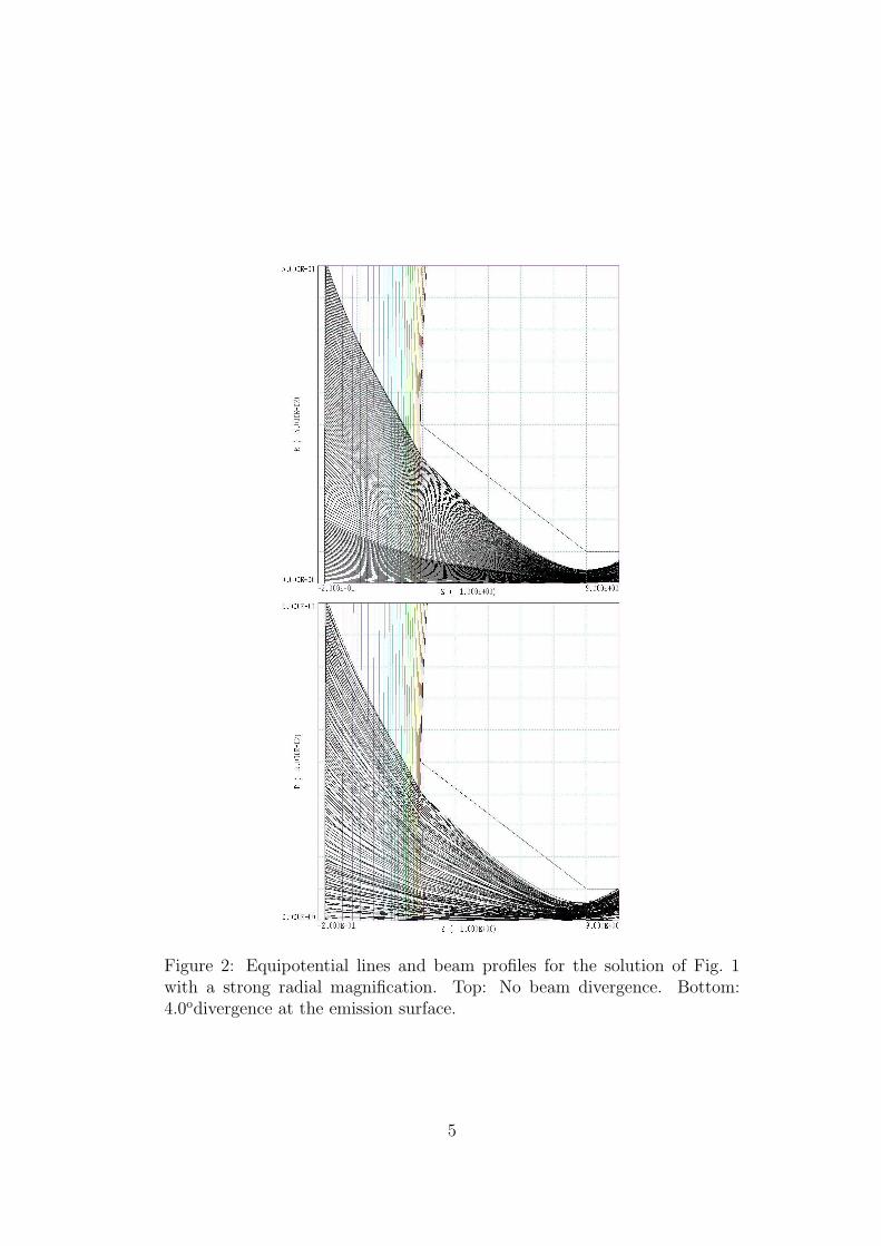
on the final geometry shown in Fig. 1. I added effects of cathode temper-ature when I was close to the desired solution. The cathode temperaturewas about 0.1 eV and the emission surface potential was 22 eV. The angulardivergence at the emission surface was therefore 0.071 radians (4.0 deg).Figure 2 shows equipotentials and model particle orbits for the working ge-ometry without and with divergence. Note the effect of field curvature at theextraction aperture. The root-mean-squared wait radius at 7.75 cm from thecathode surface was 0.018 cm.
To conclude the gun design, I added a gap between the cathode edgeand focusing electrode consistent with manufacturing tolerances. Figure 2shows a detail of the mesh near the cathode edge. In the initial run, themarked point was at same axial location as the cathode edge. In this case,the gap caused enhanced current and defocusing at the edge. I moved thepoint forward until the total current and beam envelope was the same as theideal solution. I then put a radius on the sharp edge at the anode aperturefor an estimate of the peak electric field on the anode. Figure 4 shows that|E| on the anode was less than 250 kV/cm. The maximum field stress on thenegative electrodes was in the range 50-60 kV/cm.
4
Figure 2: Equipotential lines and beam profiles for the solution of Fig. 1with a strong radial magnification. Top: No beam divergence. Bottom:4.0odivergence at the emission surface.
5
Figure 3: Detail of the mesh showing the gap between the cathode andfocusing electrode.
Figure 4: Plot of |E| near the tip of the anode extension.
6
3 Focusing solenoid
The minimum inner radius of the focusing solenoid coil was 2.22 cm (0.32 cmthick mandrel over a vacuum tube of radius 1.90 cm). The beam pulselengthin the low duty cycle system was a few µs. Therefore, I considered a pulsedmagnet coil to minimize size and complexity. An iron shield is essential toensure that field level is small at the cathode and that field transition atthe beam waist has a short axial length. The coil pulselength must be longenough to guarantee a uniform field distribution in the iron so that the fieldprofile is close to the code prediction. The time ∆t for a pulsed magneticfield to penetrate to a depth δ into a non-laminated iron shield is givenapproximately by:
∆t ∼= δ2µ0µr
2ρ. (4)
In the equation µr is the relative magnetic permeability of the iron and ρis the volume resistivity. In 1018 steel, the parameters are µr
∼= 1000 andρ = 1.01 × 10⁻⁷ Ω-m. For a shield thickness δ = 0.0075 m, Eq. 4 predictsthat ∆t ∼= 0.35 s. To be conservative, I assumes a 2.5 s pulselength in thefollowing calculations.
Figure 5 shows the dimensions of the solenoid determined from an extndedset of calculations. In the reference frame of the r-z plot, the upstream faceof the coil is at position z = 0. The coil length of 15.24 cm (6.00”) gives a flatfield region (±0.5 %) about 10.0 cm (3.94”) in length. The coil inner radiusis Ri = 2.22 cm and outer radius is Ro = 4.22 cm. The magnetic shield hasthickness 0.75 cm. The large shield opening on the downstream end allowsinsertion of microwave experiments. The shield has a small opning on theupstream side (0.3 cm radius) to ensure 1) isolation of cathode, 2) a sharptransition at the beam waist, and downstream field uniformity.
With a drive current of 38,000 A-turn, the solenoid produces a field B0 =0.312 tesla. The blue curve in Fig. 6 shows the axial variation of on-axis field,Bz(0, z). Note the broad-scale field variation at the open downstream end.The field profile would be the same at the upstream end without the radialshield extension. Such a profile Would give significant field at the cathodeand poor beam convergence. Figure 7 shows the variation of |B| near theupstream end of the coil. Field values are well below saturation over thevolume of the shield, confirming that the 0.75 cm thickness is sufficient.
We assume that coil is wound with #16 enameled copper magnet wire.Wire of this gauge is easy to wind, ensures a large number of turns for fielduniformity, and has a moderate resistance. The corresponding drive voltageis well within capacity of the insulating enamel. The following Internet sitegives useful data for magnet wire:
7
Figure 5: Transport solenoid assembly with coil highlighted. Horizontal gridspacing: 2.0 cm. Vertical grid spacing: 1.0 cm.
Figure 6: Variation of on-axis magnetic field, Bz(0, z). The surface of thecathode is at position z = 0.0. Solid blue curve: baseline design. Dashed redcurve: gap of width 0.16 cm in radial shield extension.
8
Figure 7: Spatial variation of |B| near the solenoid entrance, values in tesla.
http://www.reawire.com/ind_dims_choose.asp
The nominal diameter of bare #16 wire is 0.0508”. A typical diameter withinsulation is 0.0524”. The wire resistance is 4.018 Ω/1000 ft. For the baselinecoil dimensions, there are approximately 114 turns in each of 15 radial layers.The total number of turns is N = 1710. The drive current to achieve 38,000A-turns is I = 22.2 A. The total wire length in the coil is given by:
L ∼= 2πRi +Ro
2N. (5)
Inserting coil dimensions, we find L = 346 m or 1135 ft. The total coilresistance is R = 4.56Ω. The drive voltage is V = 101.2 V and the resistivepower dissipation is 2248 W. The total input energy during a 2.5 s pulse isU = 5620.0 J.
The bare wire radius of 0.0645 cm corresponds to a cross-section area of1.308× 10−2 cm2. Taking a length L = 3.46× 104 cm, the volume of copperin the coil is 452.0 cm3. With density 8.96 gm/cm3, the mass of copper inthe coil is M = 4054.0 gm. Copper has a specific heat Cp = 0.38 J/gm-oC.The expected temperature rise in the wire is
∆T ∼= U
CpM. (6)
9
Figure 8: Self-consistent Trak solution for beam motion in the gun, matchingregion and transport solution. Plot shows model particle orbits and equipo-tential lines with a 14:1 radial magnification.
Inserting coil values in Eq. 6, we find a relatively small temperature difference∆T = 3.7 oC (6.5 oF).
4 Beam matching calculations
Figure 8 shows a complete self-consistent solution combining the gun de-scribed in Report 1 with the new solenoid. Note that there is a strong radialmagnification – the radial extent of the plot is 1.0 cm and the axial lengthis 14.0 cm. The total drive current is 38,000 A-turn and the coil has beendisplaced +7.5 cm along the axis. This means that the upstream face of theiron shield is 6.75 cm from the cathode surface and the coil starts at z =7.50 cm. Figure 9 is a true scale representation of the complete system witha superposition of gun electrodes and the solenoid assembly.
To conclude, I checked the effects of two variations in the system. The
10
Figure 9: True-scale representation of the system showing the gun electrodesand components of the solenoid assembly.
11
first was the possibility of fabricating the upstream radial extension of themagnetic shield as a separate piece inside the vacuum tube. This arrangementleaves a gap of 1/16” (0.16 cm) in the magnet circuit (the thickness of thevacuum chamber wall). The dashed red line in Fig. 6 shows the resulting on-axis field variation. Some flux has been forced upstream and field uniformitynear the transition has been degraded. Nonetheless, there was little effecton the beam solution. Therefore, the geometry remains as an option if itsimplifies design of the system.
Finally, Figure 10 shows the effect of axial displacements of the solenoidassembly. A position error of 0.5 cm results in mismatching with large oscil-lations of the beam envelope. The position of the solenoid should be accutateto better than ±1.0 mm. After analysis of series of runs with displacementsfrom 7.0 to 8.0 cm in 0.25 cm steps, I expect that the ideal solenoid displace-ment is close to 7.375 cm. At this setting, the distance from the cathodesurface to the upstream face of magnetic shield is 6.625 cm.
12
Figure 10: Beam envelope variations with changes in axial solenoid position.Distance from cathode surface to coil. Top: 7.0 cm. Middle: 7.5 cm. Bottom:8.0 cm.