Proceedings Paper Formatting Instructions – 1 – Rev. 10/2015

Two and Three-Dimensional CFD Modeling of the Inlet Energy Dissipator of a laboratory flume.

Jorge Alejandro Mora, MSc.,1 Germán Ricardo Santos Ph.D.,2 and

Antonio Arenas Ph.D.,3

1 Master of Science Graduate Civil Engineering Department, Escuela Colombiana de Ingeniería, Autopista Norte Ak 45 No 205-59, Bogotá; e-mail: alejo.guitar@hotmail.com 2 Professor Civil Engineering Department, Escuela Colombiana de Ingeniería, Autopista Norte Ak 45 No 205-59, Bogotá; e-mail: german.santos@escuelaing.edu.co 3 Adjunct Assistant Professor, Department of Civil and Environmental Engineering, Univ. of Iowa, Iowa City; e-mail: tonoarenas@hotmail.com ABSTRACT The subject of this study is the two and three dimensional CFD modeling of the inlet and the free surface steady flow in the Escuela Colombiana de Ingeniería laboratory flume and the comparison with experimental measurements. The experimental setup includes a transitional structure and a ramp. The former’s function is to dissipate the energy of the incoming flow while the latter helps redirect the streamlines of the flow. The ANSYS FLUENT CFD software was used. The water-air interface was modeled using the volume of fluid method (VOF) and the turbulence by the "Baseline (BSL) k-" method. The topologies analyzed included scenarios with and without the energy dissipation structure and the ramp. The water surface elevation, the mechanical energy, the flow symmetry, the velocity profile and the static pressure were the main parameters used to test the computational models with the experimental data. INTRODUCTION Typically, engineers design hydraulic structures based on empiric relationships. In such cases the validity of the results is limited given that certain physical phenomena are not taken into account. Nowadays, 2D and 3D mathematical models can provide information about what will happen in an existing or modified hydraulic structure given certain proposed scenarios (Butler and Davies, 2011). In the present paper, the steady flow in the new artificial channel of the Escuela Colombiana de Ingeniería is analyzed using computational fluid dynamic models in one, two and three dimensions. For the 2D and 3D models the ANSYS Fluent version 15 is used, while elementary numerical methods are employed in the development of the 1D model.

Proceedings Paper Formatting Instructions – 2 – Rev. 10/2015

PHYSICAL MODEL The motivation for this study stems from the difficulties found in the construction of a new laboratory flume at the Escuela Colombiana de Ingeniería Julio Garavito. We have easy access to high-quality data in a controlled environment. The channel itself has a rectangular shape with a width of 38.7 cm meters, a length of 5.05 m and a variable slope. An elevated tank delivers water to a 4” PVC pipe connected to a flexible hose. The hose then serves as an inlet pipe for the main channel. Its flexibility ensures that a change in the slope of the channel does not disturb the water supply. The flow and the slope used for the analysis were 18.21 L/s and 1%, respectively.

The flow regime generated under these conditions is supercritical. Additionally, the interior of the channel contains a transitional structure, with length of 96 cm, whose function is to dissipate energy and consequently to delivers calm waters to the main channel. (see Figure 1).

Figure 1. ECIJG Laboratory flume and energy dissipater.

TWO- AND THREE-DIMENSIONAL MODELING The Navier-Stokes equations were solved for a steady incompressible multiphase flow taking into account both air and water flow by the finite volume method implemented in ANSYS FLUENT. The computational domain is discretized into a series of finite volume control (cells). The equations of conservation of mass and momentum are solved for each cell. (Versteeg, and Malalasekera, (2007). The multiphase flow was computed by solving the Reynolds-averaged Navier-Stokes equations using the baseline (BSL) k-turbulence model (Menter,1994). This model blends the standard k-model with the k- and also considers the turbulent kinetic energy (k) but uses specific rate of dissipation (instead of the dissipation (). It combines the free independence of the k-in the far field and the robustness of the k- in the near wall region. To model the water-air interphase the VOF formulation was employed. It solves a single set of momentum equations and tracks the volume fraction of the fluids through the domain. The

Proceedings Paper Formatting Instructions – 3 – Rev. 10/2015

details of the numerical approximations employed for each of the terms in the governing equations is presented in Table 1.

Table 1. Discretization methods Pressure- velocity coupling

Scheme SIMPLE Spatial Discretization Method

Gradients Least squares cell based Pressure Body force weighted

Momentum First order upwind Volume fraction Modified HRIC

Turbulent kinetic energy First order upwind Specific dissipation rate First order upwind

The simulations were ran on a personal computer with a Intel® Core™ i7 processor –

4700HQ CPU @ 2.40GHz - 2.39GHz, 4 nucleus and 8 logic processors, 16 GB of RAM memory and a graphic card NVIDIA GEFORCE GTX 760M.

The ANSYS Mesh-Workbench generator was used for the creation and design a structured

rectangular grid for the two dimensional grid. The ICEM CFD generator was used to implement a hybrid grid based on the Delaunay method for the three dimensional case. It has tetrahedral cells on the boundaries and hexagonal cells on the center (see Figure 2). The hybrid grid was selected given the complex geometry in the area where the energy dissipator is located and its surroundings. To have an adequate resolution of the flow in the high pressure gradients recirculation region, the height of the first cell was chosen such that the value of y+ would be between one and 10. In the fully developed turbulent flow region, the y+ was between 30 and 500.

Figure 2. Structured grid for 2D modelling (left) and hybrid grid for 3D modelling (right)

Four topologies were analyzed. The first one correspond to the channel with a long ramp

and was analyzed combining one and two dimensions models. The label “T0” was given to this topology. The other three topologies were modelled using 3D modelling. “T1” refers to the model

Proceedings Paper Formatting Instructions – 4 – Rev. 10/2015

without the energy dissipater and no entry ramp. Topology “T2” consists of the energy dissipater and no ramp, while “T3” includes both the ramp and the energy dissipater as part of the model. Table 2 details the number of cells used for each topology, the computational cost of running the model and the iterations required.

Table 2. Discretization methods

Topology Number of cells Computational time (hours) Iterations

T0 channel long ramp 104800 2.5 6000 T1 no dissipater no ramp 1341579 10 4350 T2 dissipater and no ramp 1656589 10 7000

T3 dissipater and ramp 1656580 10.23 7000 Residuals of the continuity equation, velocity components, turbulent kinetic energy (k),

specific rate of dissipation (and volume fraction (VOF), the water mass flow at the channel’s outlet and the static pressure were monitored to assure that for the final solution, the changes between iterations were less than 10-3 or 10-5, accordingly to the variable.

The volumetric flow, the static pressure and the water surface elevation were the variables

selected to make the comparison between the numerical results and the measured values at nine control sections (Figures 3 and 4). The confidence interval was established at 4%.

Figure 3. Control sections placement for the T1 scenarios.

Proceedings Paper Formatting Instructions – 5 – Rev. 10/2015

Figure 4. Control sections placement for the T2 and T3 scenarios.

Boundary conditions: The boundary conditions employed for the modeling of the Energy dissipator and the flume in the present study are shown in Figures 5 and 6 and described below.

Wall: No slip conditions were used; all flows perpendicular to the wall were set equal to zero. Additionally, the roughness height was assumed to be 0.008mm corresponding to smooth materials (glass, PVC, aluminum).

Figure 5. Boundary conditions for the 2D modelling of the laboratory flume

Mass flow inlet: Both air and water mass flow, as well as the turbulent intensity and

hydraulic radius are specified.

Pressure at the outlet: Atmospheric pressure at the outlet is assumed thus the gage pressure at the channel’s exit and at the top boundary are set to zero.

Proceedings Paper Formatting Instructions – 6 – Rev. 10/2015

Figure 6. Boundary conditions for 3D modelling.

RESULTS Comparison between the measured and the modeled water profile. As a preliminary analysis it is possible to compare the measured and modeled water profiles across the channel employing a visual comparison. This is done by superimposing one water profile onto the other. The results of this procedure are shown in Figure 7. In general, this analysis shows that the modeled water profile is similar to the measured levels with a notable exception; in the region corresponding to the energy dissipator, the measured data reveal that the flow is pressurized. This phenomenon is not present in the numerical model.

Figure 7. Measured and simulated Water profiles. Central axis, discharge = 18.21 lps.

The same graphical method was employed for the 1D and 2D models with and without the energy dissipator (Figure 8). The 1D modeling was done by solving the gradually varied flow differential equation by a standard fourth order Runge Kutta method. These models proved to be an asset when modeling non turbulent flow in a sufficiently long rectangular channel. Compared to the 3D models, the results did not reveal significant shortcomings. All the models showed the same kind of displacement of the critical depth for the different topologies, while the 1D and 2D

Proceedings Paper Formatting Instructions – 7 – Rev. 10/2015

models more adequately predicted the location of the critical depth for the topology that included both the ramp and the energy dissipater. According to literature where the critical depth occurs the specific energy and specific force of the flow are at its minimum, however, in the present study, the flow reached its critical depth closer to the entry of the channel than expected.

(a) (b)

(c) (d)

Figure 8. Water profile comparison for Q=18.21 lps and Void fraction =0.5 (a) 1D and 2D (b) no dissipater and no ramp (c) dissipater and no ramp (d) dissipater and ramp

Mechanical energy. The variations in mechanical energy between the sections of the channels for each topology and discharge were analyzed to determine the behavior of the flow under the different topologies. The total mechanical energy was calculated according to the following equation

ℎ = ℎ + ℎ + ℎ + ℎ Where h is the total mechanical energy or head, ℎ the piezometric head, ℎ the average kinetic energy head, ℎ the turbulent kinetic energy head and, ℎ the energy losses due to friction. Given that an energy dissipator and a ramp were implemented before the rectangular channel, the turbulent kinetic energy parameter was important to quantify the reduction in the chaotic flow observed by Rodriguez and Camargo (2013). The potential energy, average kinetic energy and

Proceedings Paper Formatting Instructions – 8 – Rev. 10/2015

total energy parameters were not useful in that analysis given that the dissipation of energy occurs in all the tested topologies regardless of the presence of the energy dissipator or the ramp. (Figure 9).

(a) (b)

(c) (d)

(e) Figure 9. Mean values of the(a) piezometric head “hEp”, (b) kinectic energy head “hEc”, (c), total head “h” ,(d) friction head “hf”, (e) turbulent kinetic energy head “hK” (e), for each

section and each topology. Flow symmetry. Model results show that the symmetry of the primary and secondary flows varies with the magnitude of the discharge for the topologies T1, T2 and T3 and support the decision to model the whole channel from the start.

Proceedings Paper Formatting Instructions – 9 – Rev. 10/2015

The results of the modeled scenarios showed an axis-symmetrical distribution of the skin friction coefficient (Cf) in the bed of the channel from section S8 to S10 for all the tested topologies. The variations that might challenge the aforementioned conclusion were deemed insignificant compared to the distribution of the primary and secondary flows. Furthermore, the distribution of the local friction coefficient was found to be strongly related to the distribution of the primary and secondary flows near the bed of the channel (Figures 11 and 12).

The analysis of the streamlines revealed an axis-symmetrical flow in the T1 and T2 topologies. This was not the case for the T3 topology; as evidenced by the photographical record (Figure 13). In this topology, the lateral distribution of the form is not symmetrical, a dominant flow moves in the direction of the main flow by the right margin of the channel. This phenomenon was effectively represented by the 3D model.

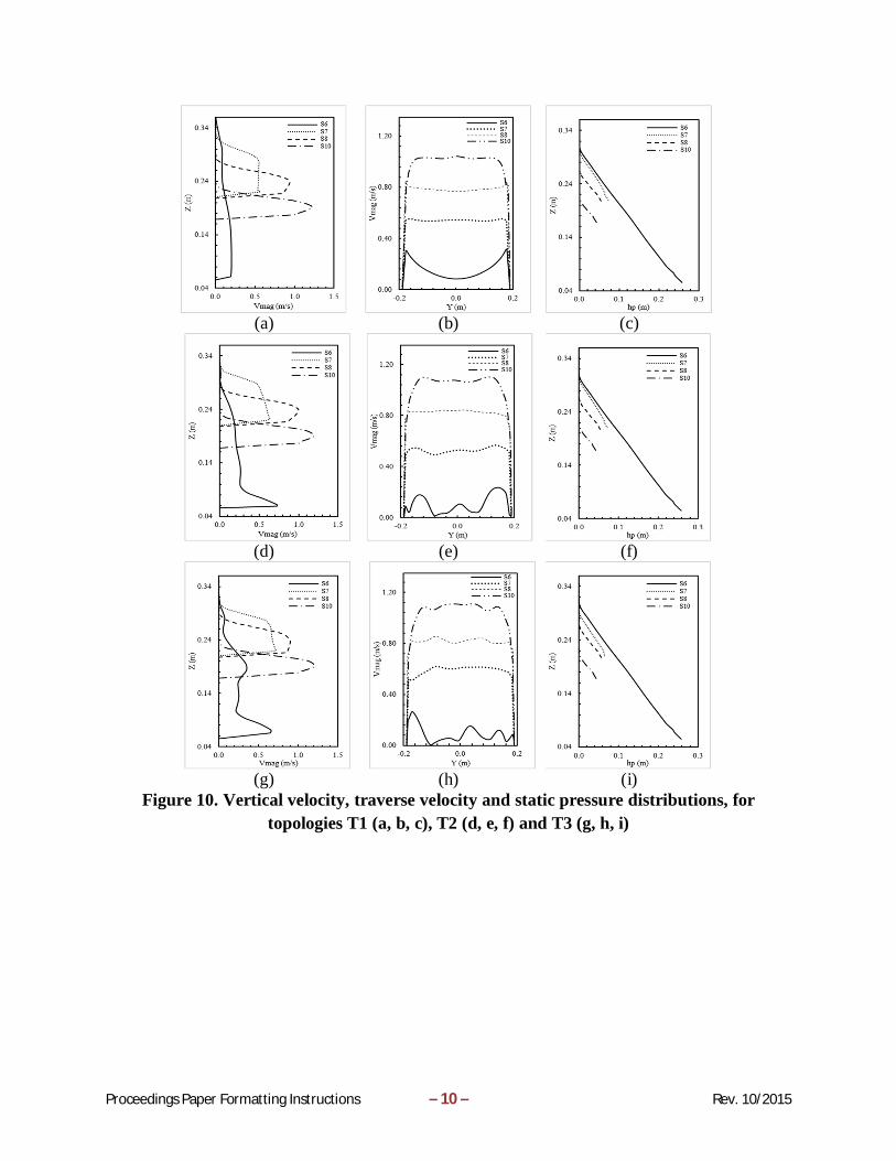
Velocity profiles. Vertical velocity profiles predicted by the model do not always display a logarithmic shape. At sections S6 (in the tank) and S7 (upstream end of the flume) for topologies T1, T2, and T3, model predictions deviate from the log-law suggesting that the boundary layer theory does not apply. In contrast, numerical results at sections S8 and S10 (both located in the flume) reveal a logarithmic velocity profile (see Figure 10).

Location along the flume influences the shape of the traverse velocity profiles. Clearly defined and close to symmetrical profiles are predicted by the model at sections S7, S8, and S10 for topologies T1, T2, and T3. Conversely, the profile at section S6 (upstream end of the flume) displays a different shape with this pattern being more apparent for topologies T2 and T3.

Static pressure profiles. The distribution profiles of the static pressure in the vertical sections S6, S8 and S10 in the topologies T1, T2 and T3 show, with minor divergences in the behavior near the channel bed, a linear relationship between the depth in the channel and the pressure exerted by the fluid. An increase in the pressure follows an increase in the depth. This is the expected behavior according to hydrostatic pressure theory. In the vertical sections S7 for the T1 and T2 topologies this pattern is not observed. A distortion of the linear relationship can be identify in deeper regions where a slight curvature can be observed. This distortion does not occur in the T3 topology suggesting that the ramp reduces the streamlines curvature and yields the formation of hydrostatic pressure profiles along the channel (see Figure 10).

Proceedings Paper Formatting Instructions – 10 – Rev. 10/2015

(a) (b) (c)

(d) (e) (f)

(g) (h) (i)

Figure 10. Vertical velocity, traverse velocity and static pressure distributions, for topologies T1 (a, b, c), T2 (d, e, f) and T3 (g, h, i)

Proceedings Paper Formatting Instructions – 11 – Rev. 10/2015

(a) (c) (e)

(b) (d) (f)

Figure 11. Primary (U) and secondary (VW), in sections 7 y 8 for topologies T1 (a, b), T2 (c, d) and T3 (e, f).

Future Work Based on the long computational times required in the modelling, it would be useful for future two and three dimensional simulations scenarios the implementation of a computer cluster to reduce the computational cost of running the simulations. Additionally, time should be spent performing additional analysis such as the grid dependency in order to reduce the uncertainty of the results of the simulation.

Transductors and an ultrasound sensor should be installed in the laboratory flume in regions where it is suspected that a hydrostatic profile is not being formed, in order to have more accurate data to compare with the simulated scenarios. Furthermore, the use of apparatus that can measure turbulence recommended by Nezu (2005) are necessary for the calibration of turbulence models. The ultrasonic current measuring device, the electromagnetic current measuring device, the hot film anemometer (HFA), the acoustic Doppler velocimeter (ADV), The laser Doppler anemometer (LDA) or the laser Doppler velocimeter (LDV), are all examples of such devices.

Proceedings Paper Formatting Instructions – 12 – Rev. 10/2015

CONCLUSIONS It was possible to accurately represent the free surface steady flow in the ECI No.2 channel through the use of the computational fluid dynamics software ANSYS FLUENT and the data obtained in the laboratory. The 1D, 2D and 3D models showed a displacement of the position in which the critical depth occurs in the direction of the flow. The displacement was found to be affected by the entry point structure of the water that enters the main channel. The displacement was the highest when a 90° step was used, while a ramp with an 18.43° slope was found to cause the least displacement. Furthermore an energy dissipation structure proved to significantly reduce the magnitude of the displacement.

Topology T1 dissipates the energy of the incoming flow given that the ascending flow meets first with dammed water and then with the atmosphere. The flow then freely falls and follows the normal flow direction. The flow in this instance continues to be chaotic. By including an energy dissipating transitional structure and a ramp the flows achieved uniformity sooner. The turbulent kinetic energy was identified to be responsible for the initial chaotic condition of the flow. Between sections S6 and S9, where the flows becomes uniform, the magnitude of this type of kinetic energy decreases continuously.

The 3D simulations were used to analyze the symmetry of the flow. The results of this

analysis could have big repercussions for future simulations as the “Symmetry” tool in ANSYS FLUENT software can reduce the computational cost of the simulations by assuming mirror symmetry. It was found that the flow is not symmetrical in all cases; the water had tendency to flow towards the right side of the channel when the energy dissipator was used. Following the results of this analysis future investigations to optimize the transitional structure are encouraged.

According to the results of the work in the laboratory and the 1D, 2D and 3D models, it was found that the use of ramps and structures that reduce the energy of the incoming flow are recommended as they reduce the length it takes the flow to reach uniformity.

Proceedings Paper Formatting Instructions – 13 – Rev. 10/2015

(a) (b)

(c) (d)

(e) (f)

(g) (h) (i)

Figure 12. Secondary flow influence on the skin friction coefficient distribution in

topologies T1 (a, b, g), T2 (c, d, h) and T3 (e, f, i).

Proceedings Paper Formatting Instructions – 14 – Rev. 10/2015

(a) (b)

(c) (d)

(e) (f)

Figure 13. Streamlines, streaklines and photografies for topologies T1 (a, b), T2 (c, d) and T3 (e, f). Figure b y d (Rodríguez and Camargo, 2013).

REFERENCES Nezu, I. (2005). “Open-Channel Flow Turbulence and Its Research Prospect in the 21st Century”

Journal of Hydraulic Engineering, ASCE, 229-246. Andersson, B., Andersson, R., Hakansson, L., Mortensen, M., Sudiyo, R., and Van Wachem, B.

(2012). Computational Fluid Dynamics for Engineers, New York, Cambridge University Press.

ANSYS, Inc. (2013). “Ansys help 15.0, Fluent”, Canonsburg, Pensilvania, Estados Unidos.

Proceedings Paper Formatting Instructions – 15 – Rev. 10/2015

Bakker, A. (2012). “The Colorful Fluid Mixing Gallery. Obtenido de Course materials for the Computational Fluid Dynamics (ENGS 150)”, Dartmouth College from 2002-2006, <http://www.bakker.org/dartmouth06/engs150/> (Mar. 12, 2015).

Butler, D., & Davies, W. J. (2011). Urban drainage. Abingdon. Taylor & Francis Group. Cengel, Y. A., and Cimbala, J. M. (2006). Mecánica de fluidos, Fundamentos y aplicaciones,

México, D.F., McGraw-Hill/Interamericana Editores, S.A. de C.V. Chow, V. T. (1994). Hidráulica de canales abiertos, (Juan Saldarriaga, Trads.), Santafé de Bogotá,

Mac Graw-Hill Interamericana S.A. Gautam, B., & Vinayak, E. (2002). Turbulent Flows: Fundamentals, Experiments and Modeling,

Kanpur, India, Alpha Science International Ltd. Mora Uscátegui, J. A. (2017). Modelación hidrodinámica Bi y Tridimensional de dos canales con

disipador de energía del laboratorio de la Escuela Colombiana de Ingeniería utilizando ANSYS FLUENT, Escuela colombiana de ingeniería Julio Garavito, Maestría en recursos hidráulicos y medio ambiente, Bogotá.

Rodríguez Cárdenas, H. S., and Camargo, S. A. (2013). Diseño y construcción de un dispositivo de disipación de energía a la entrada del canal experimental de pendiente variable de la ECI, Escuela colombiana de ingeniería Julio Garavito, Especialización en recursos hidráulicos y medio ambiente, Bogotá.

Versteeg, H. K., and Malalasekera, W. (2007). An Introduction to Computational Fluid Dynamics, the finite volume method, Harlow, Pearson Education Limited.