UNCLASSIFIED AD NUMBER ADA800273 NEW LIMITATION CHANGE TO Approved for public release, distribution unlimited FROM Distribution authorized to DoD only; Administrative/Operational Use; AUG 1951. Other requests shall be referred to David Taylor Model Basin, Washington, DC. Pre-dates formal DoD distribution statements. Treat as DoD only. AUTHORITY DWTNSRDC ltr dtd 23 Feb 1983 THIS PAGE IS UNCLASSIFIED
Transcript
UNCLASSIFIED
AD NUMBER
ADA800273
NEW LIMITATION CHANGE
TOApproved for public release, distributionunlimited
FROMDistribution authorized to DoD only;Administrative/Operational Use; AUG 1951.Other requests shall be referred to DavidTaylor Model Basin, Washington, DC.Pre-dates formal DoD distributionstatements. Treat as DoD only.
AUTHORITY
DWTNSRDC ltr dtd 23 Feb 1983
THIS PAGE IS UNCLASSIFIED
Reproduced by
- nCTIll flL. fl .0oB D VIfnfTIS0ff1,CWRIGHT-PATTERSON AIR FORCE BASE- DAYTON OHIO
Eu E
"NOTICE: When Government or other drawings, specifications or
other data are used for any purpose other than in connection witha definitely related Government procurement operation, the U.S.Government thereby incurs no responsibility, nor any obligationwhatsoever; and the fact that the Government may have formulated,furnished, or in any way supplied the said drawings, specificationsor othdr data is not to be regarded by implication or otherwise asin any manner licensing the holder or any other person or corpora--
-tion, or conveying any rights or permission to manufacture, use orsell any patented invention that may in any way be related thereto."
UNCLASS.IFIED
NAVY D)EPARTMENT ,o
THlE DAVID, W- TAYLOR MJELBASIN
WASHINGTON 7. D9C-.
THE AXIALLY SYMMETRIC POTENTIAL FLOW ABOUT
ELONGATED BODIES OF REVOLUTION
by
L. -Landweber
August 1951 Rooort 761
NS 115-084
SEP 10 1951INITIAL DISTRIBUTION
Copies
17 Chief, BuShips, Project Records (Code 324),2for distribution:5 Project Records3 Research (Code 300)2 Applied Science (Code 370)2 Design (Code 410)2 Preliminary Design (Code 420)1 Propellers and Shafting (Code 554)1 Technical Assistant to Chief of the Bureau (Code 106)1 Submarines (Code 515)
5 Chief, BuOrd, Underwater Ordnance (Re6a)1 Dr. A. Miller
3 Chief, BuAer, Aerodynamics and Hydrodynamics Branch (DE-3)
4 Chief of Naval Research, for distribution:3 Fluid Mechanics (N426)I Undersea Warfare (466)
4 Commander, U.S. Naval Ordnance Laboratory, Mechanics Division,White Oak, Silver Spring 19, Md., 1 for Dr. Max Munk
2 Commander, Naval Ordnance Test Station, Inyokern, China Lake, Calif.,1 for Underwater Ordnance Division, Pasadena
1 Commanding Officer, Navy Underwater Sound Laboratory, Fort Trumbull,New London, Conn.
1 Librarian, American Society of Mechanical Engineers, 29 West 39th St.,New York 18, N.Y.
1 Librarian, American Society of Civil Engineers, 33 West 39th St.,New York 18, N.Y.
1 Director, U.S. Waterways Experiment Station, Vicksburg, Miss.
1 Dr. G.B. Schubauer. National Bureau of Standards, Washington, D.C.
3 Director, Institute for Fluid Dynamics and Applied Mathematics,University of Maryland, College Park, Md , I for Dr.. Weinstein and1 for Prof. R. Myers, Physics Dept.
1 Prof. R.A. Dodge, Engineering Mechanics Department, University ofMichigan, Ann Arbor, Mich.
2 Editor, Applied Mechanics Reviews, Midwest Research Institute,4049 Pennsylvania, Kansas City 2, Mo.
1 Editor, Aeronautical Engineering Review, 2 East 64th St., New York21, N.Y.
1>es
1 Editor, Bibliography of, Technical Reports, Office of TechnicalServices, U.S. Department of Commerce, Washington 25, D.q.
1 Editor, Technical Data Digest, Central Air Documents Office, Wright-Patterson Air Force Base, Dayton, Ohio
2 Dr. A.T. Ippen, Director, Hydrodynamics Laboratory, Department ofCivil and Sanitary Engineering, Massachusetts Institute of Tech-nology, Cambridge 39, Mass.
1 Director, Institute for Mathematics and Mechanics, New York Univer-sity, 45 Fourth Ave., New York 3, N.Y.
1 Dr. C.A. Wright, Department of Hydraulic and Sanitary Engineering,Polytechnic Institute of Brooklyn, 99 Livingston St., Brboklyn 2,N.Y.
1 Prof. R.G. Folsom, Department of Engineering, University of Cali-fornia, Berkeley 4, Calif.
1 Prof. C.W. Harris, Department of Civil Engineering, University ofWashington, Seattle 5, Wash.
1 Prof. S.A. Guerrieri, Division of Chemical Engineering, Universityof Delaware, Newark, Del.
Illustrative Example ....... ......................... ... 21
Error in Determination of p/q ...... .. .................... 33
Comparison with Kirmin and Kaplan Methods ...... .............. 34
SOLUTION BY APPLICATION OF GREEN'S THEOREM ... ............... .. 34 1General Application to Problems in Potential Theory .... ......... 34An Integral Equation for Axisymmetric Flow ..... .............. 35
Kennard's Derivation of the Integral Equation ... ........... .. 38
A First Approximation ..... ... ...................... . 38
Solution of Integral Equation by Iteration ............... ... 39
Numerical Evaluation of Integrals ...... .................. .. 40
Illustrative Example ....... ......................... ... 42
An iteration formula for Fredholm integral equations of the first kind is ap-
plied In two new methods for obtaining the steady, irrotational, axisymmetric flow of
an inviscid, incompressible fluid about a body of revolution. In the first method a
continuous, axial distribution of doublets is sought as a solution of an integral equa-
tion of the A kind. A method of determining the end points and the initial trends
of the dbstri1I n, and a first approximation to a solution of the integral equation aregiven. This approximation is then used to obtain a sequence of successive approxima-
tions whose successive differences furnish a geometric measure of the accuracy of an
approximation. When a doublet distribution has been assumed, the velocity and pres-
sure can be computed by means of formulas which are also given.
In the second method the velocity is given directly as the solution of an inte-
gral equation of the first kind. Here also a first approximation is derived and applied
to obtain a sequence of successive approximations. In contrast with the first method,
which, in general, can give only an approximate solution, the integral equation of the
second method has an exact solution.
Both methods are illustrated In detail by an example. The results are com-
pared with those obtained by other well-known methods.
UNCLASS I F I ED
ATI 115 134 (COPIES OBTAINABLE vRaw CADO)
TAYLOR, DAVID Wo, NOL BASINS WASH*, D.C. (wo RT 761)
THE AXIALY SYWECTRIC POTENTIA. FLOW ABOUT i.ONSATILD BODIESOr REVOLUTION - AND APPENDIX
LANDWEBERI L. AUG951 61PP TAL.s DIAGNS, GRAPHS
BOoIES Or REVOLUTION - AEROVYNAICS (2)AEROYNAMICs FLUID NC"ANICS (8)
UCLASSIFIED
A -,4 LL
2
INTRODUCTION
HISTORY
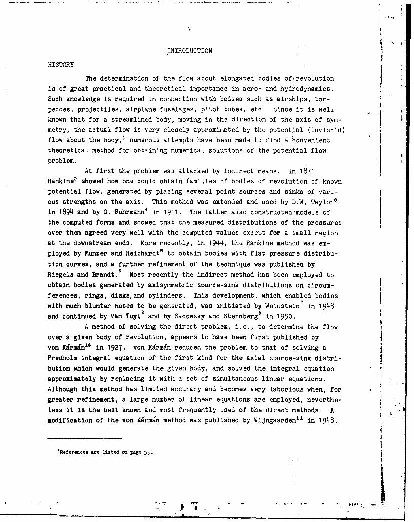
The determination of the flow about elongated bodies of~revolution
is of great practical and theoretical importance in aero- and hydrodynamics.
Such knowledge is required in connection with bodies such as airships, tor-
pedoes, projectiles, airplane fuselages, pitot tubes, etc. Since it is well
known that for a streamlined body, moving in the direction of the axis of sym-
metry, the actual flow is very closely approximated by the potential (inviscid)
flow about the body,' numerous attempts have been made to find a convenient
theoretical method for obtaining numerical solutions of the potential flow
problem.
At first the problem was attacked by indirect means. In 1871
Rankine2 showed how one could obtain families of bodies of revolution of known
potential flow, generated by placing several point sources and sinks of vari-
ous strengths on the axis. This method was extended and used by D.W. Taylor3
in 1894 and by 0. Fuhrmann4 in 1911. The latter also constructed models of
the computed forms and showed that the measured distributions of the pressures
over them agreed very well with the computed values except for a small region
at the downstream ends. More recently, in 1944, the Rankine method was em-
ployed by Munzer and Reichardt5 to obtain bodies with flat pressure distribu-
tion curves, and a further refinement of the technique was published by
Riegels and Brandt.6 Most recently the indirect method has been employed to
obtain bodies generated by axisymmetric source-sink distributions on circum-
ferences, rings, disks, and cylinders. This development, which enabled bodies
with much blunter noses to be generated, was initiated by Weinstein7 in 1948
and continued by van Tuyl8 and by Sadowsky and Sternberg 9 in 1950.
A method of solving the direct problem, i.e., to determine the flow
over a given body of revolution, appears to have been first published by
von Kirminl ° in 1927. von KErmin reduced the problem to that of solving a
Fredholm integral equation of the first kind for the axial source-sink distri-
bution which would generate the given body, and solved the integral equation
approximately by replacing it with a set of simultaneous linear equations.
Although this method has limited accuracy and becomes very laborious when, for
greater refinement, a large number of linear equations are employed, neverthe-
less it is the best known and most frequently used of the direct methods. A
modification of the von Karman method was published by Wijngaarden" in 1948.
1References are listed on page 59.
* !$ -°
3 [I
An interesting attempt to solve the direct problem was made by
Weinig12 in 1928. He also formulated the problem in terms of an Integral equa-
tion for en axial doublet distribution which would generate the given body,
and employed an iteration formula to obtain successive approximations. Since
the successive approximations diverged, the recommended proceduxve was to extra-
polate one step backwards to obtain a solution.
In 1935 an entirely different approach, in which a solution for the
velocity potential was assumed in the form of an infinite linear sum of orthog-
onal functions, was made by Kaplan1 3 and independently by Smith.1 4 The coeffi-
cients of this series are given as the solution of a set of linear equations,
infinite in number. In practice a finite number of these equations is solved
for a finite number of coefficients, and Kaplan has shown that the approximate
solution thus obtained is that due to an axial source-sink distribution which
is also determined. A simplification of Kaplan's method by means of addition-
al approximations was proposed by Young and Owen15 in 1943.
It appears to be generally agreed, by those who have tried them,
that the aforementioned methods are both laborious and approximate. Thus, ac-
cording to Young and Owen:1 5
'In every case, however, the methods proposed are laboriousto apply, and the labour and heaviness of the computationsincrease rapidly with the rigour and accuracy of the proc-ess. Inevitably, a compromise is necessary between theaccuracy aimed at and the difficulties of computation. Allthe methods reduce, ultimately, to finding in one way oranother the equivalent sink-source distribution, and it isthis part of the process which in general involves theheaviest computing."
Furthermore, a fundamental objection is that only a special class of bodies of
revolution can be represented by a distribution of sources and sinks on the
axis of symmetry. According to von Kirmn: 1 0
"This (representability by an axial source-sink distribu-tion) is possible only in the exceptional case when theanalytical continuation of the potential function, freefrom singularities in the space outside the body, can beextended to the axis of symmetry without encountering
e singular spots."
The dissatisfaction with these methods is reflected by the continuing attempts
to devise other procedures.
A new method published by Kaplan 1' in 1943 is free of the assumption3
of axial singularities and appears to be exact in the sense that the solution
can be made as accurate as desired, but the labor required for the same ac- Icuracy appears to be much greater than by other methods. The application of
the method requires that first the conform3l transformation which transforms
I+
L. I~
the given meridian profile into a circle be determined. The velocity poten- 4
tial is then expressed as an infinite series whose terms are universal func-
tions involving the coefficients of the conformal transformation. 9Kaplan'
has derived only the first three of these universal functions.
Cummins of the David Taylor Model Basin is developing a iethod based
on a distribution of sources and sinks on the surface of the given body. This
method is also exact, but the labor involved in its application has not yet
been evaluated.
Another exact method, based on a distribution of vorticity over the
surface of the body, is being developed by )r. Vandry of the Admiralty Re-
search Laboratory, Teddington, England. The methods of both Cummins and
Vandry lead to Fredhoim integral equations of the second kind, which can be
solved by iteration.
The present writer has developed two new methods, an approximate one
in which an axial doublet distribution is assumed, and an exact one based on
a general application of Green's theorem of potential theory. Both methods
lead to Fredholm integral equations of the first kind for which a solution by
iteration has been discussed by the author.'7 Indeed, the consideration of
this iteration formula was initiated in an attempt to find more satisfactory
solutions of the integral equations of vorn Karmanl ° and Weinig.' 2 These new
methods will be presented, and, by application to a particular body, compared
with other methods from the point of view of accuracy and convenience of
application.
FORMULATION OF THE PROBLEM
We will consider the steady, irrotational, axially symmetric flow
of a perfect incompressible fluid about a body of revolution. Take the x-axis
as the axis of symetry and let x, y be the coordinates in a meridian plane.
Denote the equation of the body profile by
y2 - f(x) [1
Since the flow is irrotational there exists a velocity potential *which, for axisymetric flows, depends only on the cylindrical coordinates
x, y and satisfies Laplace's equation in cylindrical coordinates
A+1(2]
5
Also, since the flow is axisymmetric, there exists a Stokes stream function
O(x, y) which is related to the velocity potential by the equations
alp at, U4 . x (3]
It is seen that Equation (2 ] may be interpreted as the necessary and suffi-
cient condition insuring the existence of the function 0. As is well known,
t is constant along a streamline and, considering the surface of revolution
generated by rotation of a streamline about the axis of symmetry, 2iro may be
considered as the flux bounded by this surface. On the surface of the given.
body and along the axis of symmetry outside the body we have 0. satis-
fies the equation
which is obtained by eliminating s between Equations [3]
The velocity will be taken as the negative gradient of the velocity
potential. Let u, v be the velocity components in the x, y directions, Then
by (3], we have
v y xj (6]
For a uniform flow of velocity U parallel to the x-axis we have
.m-Ux, (-- u9 (7]
The boundary condition for the body to be a stream surface may be
written in various ways. If the body is stationary the boundary condition is
*(x, V7FT -0 [8aJ
or, equivalently,
d S(8b
n ) .-
6
where the derivative in [8b] is evaluated on the surface of the body in the
direction of the outward normal to the body. If the body is moving with veloc-
ity V parallel to the x-axis the boundary condition becomes
--v OB,(9
where p is the angle between the outward normal to the body and the x-axis.
It is desired to obtain a solution of [2] or [4] which satisfies the
boundary conditions (7] at infinity and (8] or [9] on the body.
METHOD OF AXIAL DISTRIBUTIONS
SOURCES AND SINKS
The potential and stream functions for a point source of strength M
situated on the x-axis at x = t are
r' ' = w(-i + r [10
where
r (X- t) 2 + y2 ]
If the sources are distributed piecewise-continuously along the x-
axis between the points a and b (see Figure 1) with a strength u(x) per unit
length, the potential and stream functions are
d dt (12]
X-t~S+(t)(-l +r dt [13]
Figure I - The Meridian Plane
7
As is well known, Rankine bodies are obtained by superposition of
these flows with a uniform stream so as to obtain a dividing streamline begin-
ning at a stagnation point. Without loss of generality we may suppose this
uniform stream to be of unit magnitude. This dividing streamline is the pro-
file of the Rankine body for which, by [7], the stream function is
~ y2 +f (- + ~dt (14]2 r.
The boundary condition, Equation [8a], then gives as the impli6it equation for
the body
f' ( 1 + dt = -y2 [15]
where now Y2 - f(x) and r2 * (x-t)g + f(x). In order to obtain a closed body
the total strength of sources and sinks must be zero, i.e.,
In this case (15] becomes
,(;.t) x a t - [15a]
In general [15a] cannot be solved explicitly for f(x) when ,[t) is
given. A practical procedure for obtaining f(x) for a given x is to evaluate
the integral numerically for various assumed values of f(x) and to determine
the value which satisfies [15a] by graphical means.
-When f(x) is prescribed (15a] may be considered as a Predhols inte-
*gral equation of the first kind for determining the unknown function g(t).
This equation will not be treated. Indeed it will be shown that, when con-
tinuous distributions are considered, it is a special case of the more general
equation for doublet distributions which will now be derived.
DOUBLET DISTRIBUTIONS
kLet m(x) be the strength per unit length of a continuous distribu-
tion of doublets along the x-axis between the points a and b (see Figure 1).
The potential and stream functions may be taken as
t-X* m = (t) dt [161• i
l ~ -m - In
'I"
8
and
y2 m(t) dt [17]
The stream function for a Rankine flow now becomes
y2 + y2 f' + ) dt [18]2a rs3
Hence the boundary condition, Equation [8a), gives
M.( ) dt = 19
Here again Equation [19] may be considered as an implicit equation for the
Rankine body when m(t) is given, or as a Fredholm integral equation of the
first kind when the body profile y - f(x) is prescribed.
In ordet to show the relation between the source and doublet distri-
butions in Equations [15a] and [19], integrate by parts in [19]. We have
f dt - + , -+- dt
Hence [19] may be written as
m(t) - +JTt -rdtu+2 [20]
The interpretation of Equation [20] is that a doublet distribution of strength
m is equivalent to a source-sink distribution of strength dm/dt together with
point sources of strength m(a) and -m(b) at the end points. Hence source-sink
distributions are completely equivalent only to those doublet distributions
which vanish at the end points. This Justifies the remark in the previous
section that the integral equation for the doublet distributions is more gen-
eral than that for the source-sink distributions.
MUNK'S APPROXIMATE DISTRIBUTION
Munk"e has given an approximate solution of Equation [19] for elon-
gated bodies. His formula may be derived as follows. At a great distance
from the ends of a very elongated body, the integrand of [19], m(t)/r3, will
A00
SA r. *
peak sharply in' the neighborhood of t = x. In the range of the peak, in which
the value of the integral is principally determined, m(t) will vary little
from m(x). Also, only a small error will be introduced by replacing the lim-
its of integration by - and +cc. Hence, as a first approximation to a solu-
tion of [19], try
~dt 1m1(x)f. y~ [21]
We obtain
Ml(x) - 9[22]
a distribution proportional to the section-area curve of the body. This ap-
proximation was independently derived by Weinig12 who employed it as the first
step in a divergent iteration procedure. It has also been rediscovered by
Young and Owen'5 and Laitone'9 who have shown the accuracy of the approxima-
tion for elongated bodies by several examples.
It is apparent from its derivation that [22] also gives the asymptot-
ic radius of the half-body generated by a constant axial dipole distribution
extending from a point on the axis to infinity. It is readily seen that this
distribution is equivalent to a point source at the initial point.
As a refinement to Munk's formula, Weinblumie has used the approxi-
mation
mI(x) -.C9 [23]
where C is a factor obtained by comparison of the distributions and section-
area curves of several bodies. Weinblum's factor bears an interesting rela-
tion to the virtual mass of the body. This is seen by considering the expres-
sion for the virtual mass kIA in terms of the mass of the displaced fluid A
and the totality of the doublets,
.kA a 4*p mdx - 24
where k. Is designated the longitudinal virtual mass coefficient, and p is the
density of the fluid. But, from [23],
4orfmadx - iICf rydx a 4CA
Li - -1.. ~
10
since, for elongated bodies, a and b very nearly coincide with the body ends.
Hence
C =(1 + k) [25]
In practice an approximate value of k1 may be taken as that of the
prolate spheroid having the same length-diameter ratio as the given body. The
values of k1 for a prolate spheroid may be computed from the formula2 4
ki M [261Xl( i:~2 - Xln (X + 7X [26]
where A is the length-diameter ratio. Hence
1 a1 s/2
C- '(k ) [27]
The values of k1 versus A have also been tabulated by Lamb' and graphed byMunk. 2 1
END POINTS OF A DISTRIBUTION
A difficulty in determining the doublet distribution from Equation(19] is that the limits of integration, a and b, are also unknown. In themethod of von Kirmfin" the end points are arbitrarily chosen; Kaplan 1 takesthe end point of the distribution midway between the end of the body and thecenter of curvature at that end.
Kaplan based his choice on a consideration of the prolate spheroid.Thus the equation of the spheroid of unit length and length-diameter ratio A,extending from x - 0 to x - 1, is
9 2.~( [x)28]
The radius of curvature at x a 0 is then-a-. The exact doublet distribution,20 *
however, extends between the foci of the spheroid which are situated at dis-tances
2A
from the end points. Hence the error in Kaplan's assumption,
4 )<V'" - - 1.m-2-( +- + ...
2X 4X2 16x 2X2
diminishes rapidly with increasing X.
For the half-body generated by a constant doublet distribution (a
point source), Kaplan's assumption gives a poor approximation. Let a2 be thestrength of the distribution. Then it can easily be shown from [19] that the
source is at a distance a from the end of the body (stagnation point), and
that, if the origin is chosen at the latter point, the equation Of the half-
body is
8x 20 2 16 [
Hence the radius of curvature at the end Is 4a so that Kaplan's assumption
for the start of the distribution gives-. This is in error by 3 a.An approximate method for determining the end points of a distribu-
tion and its trends at the ends is given in Appendix 1. The given profile is
assumed to extend from x - 0 to x - 1 and to have the equation
y2 - a x + a2x2 + a3x* + ... [30]
The doublet distribution is assumed to extend from x - a to x - b, so that
0 < a << b < 1, with a near 0 and b near 1, and to have the equation
M(x) - C + C1 x + c,x' + ... [31]
Only the trends of the distribution near the origin are discussed in Appendix
1. It is clear, however, that by means of a linear transformation the equa- Ition of the given profile can be expressed so that the end points of the bodyexchange their roles. Hence the results in Appendix 1 can be applied to either6Iend of the body.
The method of Appendix 1 consists essentially of expanding the inte-
gral in (19] about the origin and equating powers of t on the two sides of the
equation to obtain a series of equations in the unknowna a, c, c , c . .By applying the first four of these equations an approximate solution is ob-
When &V a2, a , are all small in comparison with unity, an ap-
proximate solution for a is
13
4 + a2 - a a, if a Z 0 [40]
=4 + a, if a < 0 [41]
2 3
and, to the same order of approximation,al(x) =2 1 1)(a + y2)
m(T40 . +# 2- [42]
and
inca) = 2 + + a ln a -a-y, if a 3 a 0 [431
m(a) = 0, if a3 < 0 [44]
It is seen that Kaplan's assumption that a = 4 gives the principal
term of the solution in [40] or [41]. The form [42] immediately suggests a
modification and refinement of the Munk-Weinblum approximation, Equation [23],
which will be considered in the next section.
A graphical procedure for finding the roots a of Equation [35] isalso given in the Appendix. For this purpose the functions A(a), B(a),... H(a)are tabulated in Table 10.
AN IMPROVED FIRST APPROXIMATION
According to its derivation the Munk approximation could be expected
to be useful only at a distance from the end points of a distribution. It was
seen, howover, Equaticn [42], that under certain circumstances a distribution
which was a suitable approximation for the nose and tail of a body also ap-
peared as a generalization of the Nunk-Weinblum approximation, [23]. This Isuggests a procedure for obtaining an improved approximate distribution.
It is desired to obtain a distribution m(x) which satisfies the fol-lowing conditions:
r (a) n(x) assumes known values ma and mb at the distribution limits a and
b, i.e.,
mia) - m, m(b) - [451
(b) m(x) is nearly equivalent to the Munk-Weinblum approximation (23] at
a distance from the distribution limits, i.e.,
m(a)=aC? for a 4x< b
14
(c) m(x) satisfies the virtual mass relation [24] which may be written
in the convenient form
m(x)dx =(1 + k) Jy2dx (46]
It is readily verified that Condition (a) is satisfied by the
distribution
(x) C 2 + eo + e x [47]
where
e. F a[b %- + C(afb bf a)] [48]
and
e 1 b" - ma + C (f - fb)] [49]
If the linear term e o + eIx in (47] is small in comparison with m(x) at a dis-
tance from the ends, then Condition (b) Is also satisfied. Finally, Condition
(c) can be satisfied by a proper choice of C in [47]. This is accomplished by
writing m(x) in the form
mill - c( b-x f -a f b-x + -,oY- T-aa-- f~b) +F- a a B-aa b
substituting it into Equation [46], and solving for C. We obtain
jl+k adx -j-(b-a) (ma+~
y x- 7(b -a) (fa+fb)L~
SOLUTION OF INTEGRAL EQUATION BY ITERATION
Now that we have derived a good first approximation to the doubletdistribution function in the integral equation [193, it would be very desir-able to apply it to obtain a second, closer approximation. This can be accom-plished by means of the iteration formula which we will now derive.
Let ne,(x) be a known first approximation and *1 (x) the corresponding
values of the stream function *on the given profile yR = f(x). Then, from
Equation [18],
15
- W f(x) + f(x) - t- dt51
Thus 0 (x) is a measure of the error when m (t) is tried as a solution of theII
integral equation [19]. If m(t) is a solution of (19], Equation, [51] may be
written in the form
b m 1(t)-m(t)
W - f(x) 3 dt [52]
But, on the same assumptions as were used to derive Munk's approximate distri-bution, Equation (22), we obtain as an approximate solution of the integral
equation [52]
m lx) - mlx) = 0,(x) (53]
or, denoting the new approximation to mix) by m (x),
m.(x) - mj(x) - (x) (54]
Hence, from [51]
m2 (x) - m(x) +7 f(x)[.- A-)dtJ [55]
Since the foregoing procedure can be repeated successively, we obtain the iter-
ation formula
m+ Wx) = mi x) +-1 f(x) j' r d (56]
and
(i+i(x) - mi x) - -1-(x) 157]
It is seen that 0, is the value of the stream function on the given
profile corresponding to the i t h approximation m I W and hence serves as ameasure of the error when mi(t) is tried as a solution of the integral equa-
tion [19]. 1Although successfve approximations to mix) may be computed directly
from 156], an alternative form, which is both more convenient and more signif-
icant, will now be derived. From (56] we may write.
16
M(X) m(x) +- fJ - dt [56a]
Hence, deducting [56a] from [56] and making use of [57], we get
bi
,i(x) _ .(x) - - f(x) dt [58]
Also, from [57] we obtain
mi(x) m m(x) W jx [59]i-i
Thus, In order to obtain mi+l(x), we first assume an a x), then determine
tl(x) 'from [51]. V,(x), *i(x), ... can then be successively obtained from
[58], and finally m1+l(x) from [59].It has been stated that the magnitude of i,(x) is a measure of the
proximity of m (x). This property of *1 (x) can be given a geometrical in-
terpretation. Corresponding to the distribution mi(x) there is an exact
stream surface on which the stream function 0(x, y) a 0. Let An, be the
distance from a point (x, y) on the given body to this exact stream surface,
measured along the normal to the given body, positive outwards. Let ua be
the tangential component of the flow along the body. Then we have
1 81 (xy) 1 Ah*(x,y)a, = 'F n " y An I
But A*- -*r(x), since #i(x, y) - 0 on the exact stream surface. Hence
SC(x)An I a- yus(60
Since, for an elongated body, us - 1, except in the neighborhood of the stag-
nation points, it is seen that *l(x) enables a rapid estimate to be made of
the variation from the desired profile of the exact stream surface correspond-
Ing to mt(x). This is an important property because It can be used to monitor
the successive approximations. Thus, the sequence *,(x) can be terminated
when An, becomes uniformly less than some specified tolerance; or, since there
is no assurance that the infinite sequence #1 (x) converges. the sequence can
conceivably give useful results even without convergence If it Is, continued as
S17
long as Ani decreases on the average, and is terminated when the error begins
to increase and grows to an unacceptable magnitude at some point along thebody. The strong similarity between these remarks and the discussion follow-
7 ing Theorem 2 of Reference 17 should be noted.
There is also a strong similarity between the iteration formula ofReference 17 whose convergence was thoroughly discussed, and the present equa-
tion [561. An essential difference between the iteration formulas is that theformer employs the iterated kernel of the integral equation, the latter doesnot, so that the convergence theorems of Reference 17 are not applicable. Nev-Ri ertheless, it is proposed to use the form in [56] (or the equivalent iteration
formula [58]), for the following reasons:
a. The labor of numerical calculations would be greatly increased by
iterating the kernel, and even then only convergence in the mean would be
guaranteed (Theorem 4 of Reference 17).
b. The physical derivation of Equation [56] indicates that at least the
first few approximations should be successively improving.
c. The successive approximations are monitored so that the sequence can
be stopped when the error is as small as desired or, In the case of initial
convergence and then divergence, when the errors begin to grow.
VELOCITY AND PRESSURE DISTRIBUTION ON THE SURFACE
When an approximate doublet distribution mi(x) has been obtained,
the velocity components u, v can be computed from the corresponding stream
function [18]
*i(xy) - Y L dt - [611J.
from which, in accordance with Equations [5] and (6],
u= 1 + f( - m(t)dt [62].'r' ra
and~t-X
re " l(t)dt [63]V l-
*
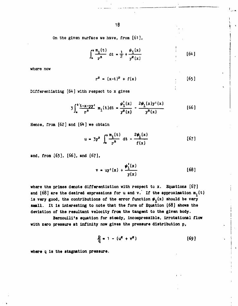
18
On the given surface we have, from [61],
2 yi(t) (x) [64
where now
r= (x-t)2 + f(x) [65]
Differentiating [64] with respect to x gives
'(x) 2*i(x)yI(x) [63 6*"t-x-y' m (t)d t - 0i(x .-~~ 'x [66]
f. r y2(x) y*(x)
Hence, from [62] and [64] we obtain
U.3y2 b mi(t) 2(x) [67f(x)
and, from [63], [66], and [67],
O4(x)
v - uy'(x) + [68]y(x)
where the primes denote differentiation with respect to x. Equations [67]
and [68] are the desired expressions for u and v. If the approximation mi(t)
is very good, the contributions of the error function *,(x) should be very
small. It is interesting to note that the form of Equation [68] shows thedeviation of the resultant velocity from the tangent to the given body.
Bernoulli's equation for steady, incompressible, irrotational flow
with zero pressure at infinity now gives the pressure distribution p,
1 -(u + va) [69]q
where q is the stagnation pressure.
119NUMERICAL EVALUATION OF INTEGRALS
In order to perform the iterations in Equations [56] and [58] and to
compute the velocity distribution it will frequently be necessary to evaluate
integrals of the form
b m ( t ) dt and b m ( t ) dt
rr
where
r, (x-t)2 + f(x)
Because in this form these integrals peak sharply in the neighborhood of t x,
especially when the body is elongated, they are consequently unsuited for nu-
merical evaluation.
A more suitable form can be obtained by means of the following trans-
formation. Let (x, y) be the coordinates of a point on the body, t the ab-
scissa of a point on the axis, 9 the angle between a line joining these two
points and the x-axis; see Figure 1. Then
x - t - y(x) cot ( [701
We may now transform the integrals so that 9 becomes the variable of integra- Ition. Then
3m(t)dt m :(t) sin 0df [71]
and
1here: t) Jm(t) sin dG [721
~where
a a arctan x ya# arctan (731
An alternate procedure, which eliminates the peak without a trnm-
formation of variables, is the following. We have -!
-m(t)t •f [m(t) +m(x)]dt+(X) dt,Sr s r r
.I !
20
and
fIm(t)dt *fY[m(t)-m(x)]dt + mx) dt
Hence
m(t)dt r ff[m(t) -m(x)] dt + m(x) (cos a - cosp) 7a
y m(t)dt f f-L[m(t)-m(x)]dt
+ m(x) [CoB a- coro -- (cosa - Coo )] [72a
Gauss' quadrature formula is a convenient and accurate method of
evaluating these integrals. The formula may be expressed in the form
jF()df - 4, RniF((n) (74]
where the t are the zeros of Legendre's polynomial of degree n and the Rniare weighting factors. These have been tabulated for values of n from 1 to16. These numbers have the properties
Rni - Rn,n-i+ 1 and f nn-+l (75]
The value of the integral given by Formula [74)] is the same as could be ob-tained by fitting a polynomial of degree 2n-1 to F(x). The values of R andnieni are tabulated in Table 1 for n - 7, 11, and 16.
When the limits of Integration are a and P, as in Equations (71 1and (72), Gauss' formula becomes
/ (O]d* -Rig-r ' n , I 1761
where
I
21
TABLE I
ABSCISSAE AND WEIGHTING FACTORS FOR. GAUSSI QUADRATURE FORMULA
We will also need the slope of the profile which, from [78], is
Y1=f'(x) -0.4 X3
- 2y (1.x4 )1/2 [82]
The profile and f(x) are graphed in Figure 2.
Y
-IId
Figure 2 - Graphs of y(x) and y2(x) for y2 (x) - 0.04(1 - x')
First let us find the end points or the distribution. We have, from[81], a1 a 0.08, a2 - -0.24, a3 - 0.32. The approximate formula (40] thena1gives a - 3.68 or 3.84, whence a - - - 0.0217 or 0.0208. An examination ofthe complete polynomial [37] with the aid of Table 10 shows that its zeros oc-cur at a - 3.65, 3.85, 12.1. In the application of Table 10 to determine theseroots the regions of possible zeros should be determined by inspection, thevalues of the polynomial in these regions calculated from Equation [37] andTable 10, and then graphed to obtain the zeros. It is seen that in the pres-ent case the approximate formula (40] would have been sufficiently accuratefor the determination of the roots near a - 4. The solution of the completepolynomial equation will always yield an additional large root, correspondingto the large root of Equation (131 ] of the Appendix; in general, however, this
root should be rejected since as wll be shown, the initial doublet distribu-tion corresponding to it is less simple than for the roots near a - 4.
--------I
23
The initial behavior of the distributions corresponding to each of
the three roots, as determined from Equations (33] through [36], and [39], is
Ishown in Table 2. It is seen from the table that the distribut on for a - 12.1
begins with practically a zero value for m(a), with a small negative slope and
with upward curvature. Since the distribution curve cannot continue very far
with upward curvature, there must be an inflection point nearby. In contrast,
the distribution corresponding to the other two roots begin with positive
slopes and downward curvatures and hence must be considered simpler. Further-
more, the distribution for the first root is considered simpler than for the
second since the distribution curves are practically identical except that,
for the second root, the curve is extended a distance Aa - 0.0011, in the
course of which m(a) changes from a positive to almost a numerically equal
negative value. If we take the point of view that the positive and negative
values of this extension counterbalance each other, the curve without the
extension, corresponding to the first root, must be considered the simplest.
Hence, for the purpose of obtaining a first approximation, we will
assume a -3.65 and, correspondingly, a - 0.022, m(a) - 0.000022. Often, as
in this case, the labor of obtaining a and ae(a) can be considerably reduced
by using the less exact equations (401 through (441 instead of [37) through
S(39]. Since, as will be seen, the iteration formulas rapidly improve upon thefirst approximation, great effort should not be expended to determine an
initial value for r(a).
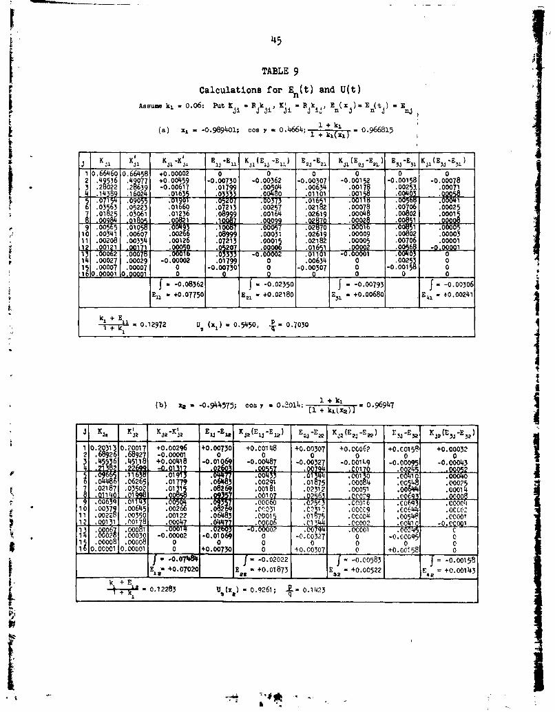
The values a - 0.022 and a(&) - 0.000022 have been derived for the
profile in the f, #-plane. The corresponding values in the x, y-plane are
a = -0.956 and ma 0.000088. By symetry we also have b = -a,%m
A first approximation can now be obtained from (47], (481, [49], and(50). Since A a 5.0, we have k, - 0.059. Also, from [78]: fa a 0.00659,
fedlxfo 0.0640, Cy'dx - 0.0637. Hence from (501, C - 0.328. Then, from (481,• £, IiI
24
eo ma - Cfa - -0.00207; from (49], eU 0. Finally we obtain from (47]
mj(x) = 0.328y2 - 0.00207 (83]
We can now apply Equation (51] and the iteration formula [58] to ob-tain the sequence of functions *,(x). Let us suppose that it is desired toobtain a distribution mi(x) whose exact stream surface deviates from the givensurface by less than one percent of the maximum radius, i.e., A4 < 0.002.Then, by [60], the sequence i(x) should be continued until b(Xi) < 0.002 Vf-xfor a S x S b, unless the error, as represented by t(x), begins to grow beforethe desired degree of approximation is attained. In the latter case the bestapproximation attainable would fall short of the specified accuracy.
The integrations in [501 and [51] may be carried out in the form[71] in terms of 9 defined in [70]. For a fixed (x, y) on the given profile,a and 9 are first computed from [73]. Then, to apply Gauss' quadrature formu-la [76], the interval is subdivided at the points Gj given by [77] and theIntegrands evaluated at these points. The corresponding values of t at whichme(t) in [51] or 0.,(t) in [58] is to be read are, from [70],
t =x - y cot Gj [70a]
Since the values t and sin * are used repeatedly in the successive itera-tions at a given (x, y), these should be stored in a form convenient forapplication.
The calculations for obtaining the integration limits a and p forseveral values of x are given in Table 3. The values of 9 from [77], and thecorr esponding values of Ra sin 0 for application of the Gauss 11 ordinateformula, and the values of t from [70a] for each x are entered as the firstthree columns in Tables 5a through 5h, in which are given the calculations for
Oj(x).In order to compute #,(x), al(t) Is computed from [83], then
m R sin * is obtained. These are tabulated in Table 5. Gauss' formula then
gives fin sine dG. is then obtained from [51]; Its graph is given inFigure 3. It is important to note that m 1(t) is obtained by calculation,rather than graphically, in this operation. This procedure is recommendedsince it gives greater accuracy in a critical step. In the subsequent opera-tions on the *s considerably less percentage accuracy is required, since the#'s are of the nature of first differences between the m's, so that graphicaloperations are sufficiently accurate.
a.- -. . C- -
25
'-.u- r~r - a -Lr-
re- 0 .- 0 0 WN 00 a+" r- r-- cyN U~ 4 N O ar- 0
_ _ _ _ _ _ _ _ _ _ _ _C_ C>U
C>\ - O ~ o~ *~ r- \,o ic--- u-\
r-~~0 af' - >-Y u 0 u, *r *r-CN C~ + r- i- r- (7\ 00Lf\
Lf - C\JIn r-\ r \0 0 0 aN N -C C C r, 0 C)\\ LN .o r-C)\00
Figure 5 - Comparison of Vklues of p/qObtained by Various Methods-! o: ,.*,
33
ERROR IN DETERMINATION OF p/q
Let A(p/q), Au, Av, and Am denote errors in p/q, u, v, and m. Then,
from [691, we have
Ak -2(u Au + v AV)
from [68], i
Av = y' Au Jand from (67] and (72], except near the stagnation points, A
Au a2 3A f Wsin 5 Od Um
y 2 J0y
Hence
A.R. 8uAm ( +q 2 +
If now we assume u a 1, y' a 0, y2 a 4m (Hunk'a approximation), we obtain
A - ar2Amq m
Thus an error of one percent In the determination of m would Introduce an
error of 0.02 in p/q.
In the foregoing example the minium value of p/q was about -0.20.
Hence an error of one percent in m would have produced an error of ten percent
in the minimum value of p/q. It was found, in fact, that the results with
Gauss' 7-ordinate rule deviated from the values of p/q given by the 11-point
rule by less than 0.003 for the entire body. The 7-point rule would have
* sufficed If an accuracy of only 0.003 in p/q were required; see Figure 5.
If greater accuracy is desired the integrals can be evaluated in the
forms 171a) and (72a]. If the latter forms are used In conjunction with the
Gauss quadrature formula the values of x should be chosen identical with thet's required by the Gauss formula. This enables the entire calculations, in-cluding the iterations and the velocity determinations, to be made arithmeti-
cally, without resort to graphical operations, so that the method becomes suit-
able for processing on an automatic-sequence computing machine. In order to
obtain sufficient accuracy In the integrations and to obtain the velocities Iand pressures at a sufficient number of points along the body a Gauss formula.
of high order should be used, say n - 16. For this reason the procedure that
has been illustrated in detail may be less tedious for manual application.
COMPARISON WITH KARNAN AND KAPLAN METHODS
In order to compare the accuracy of the Kirmain method with the pres- 4
ent one, the error function @k(x) was computed for a distribution derived by
the Kirman method, employing 14 intervals extending from -0.98 ;S x :5 0.98.
k(x) is graphed in Figure 3. It is seen that the errors are much greater
than for- the present method, especially near the ends of the body., The oscil-
latory character of 0 k(x) is imposed by the condition that the stream function
should vanish at the center of each Interval. It is conceivable that the
amplitude of the oscillations in ok(x) may remain large even when the number
of intervals is greatly increased; i.e., the Kirmin method may give a poorer
approximation when the number of source-sink segments is greatly Increased.
The pressure distribution obtained by the Kdarmn method is graphed in Figure 5.
Kaplan's first method" was also applied to obtain the pressure dis-
tribution. Kaplan expresses the potential function 0 in the form
q€- LAnqn(A) Pn{)
where X and p are confocal elliptic coordinates,
Pn(p) and Qn(A) are the nth Legendre and associated Legendrepolynomials, and the
an'S are coefficients to be determined from a set oflinear equations which express the conditionthat the given profile is a stream function.
In the present case it was assumed that 0 was expressed in terms of the first
9 Legendre functions and the AnIs determined from the conditions that the
stream function should vanish at 9 prescribed points (including the stagnation
points) on the body. The resulting pressure distribution Is also shown in
Figure 5.
SOLUTION BY APPLICATION OF GREEWS THWREN
OINAL APPLICATION TO PROBLE IN POTENTIAL THE¥RY
Let # and w be any two functions harmonic in the region exterior to
a given body and vanishing at infinity. Then, a consequence of Green-s second
identitya is
ff OLwdSmff doS (851
dn f h# .. -n
_Ali
35
where the double integrals are taken over the boundary of the body and dndenotes an element of the outwardly-directed normal to the surface S. Alsoderivable from Green's formulas is the well-known expression for a potentialfunction in terms of its values and the values of its normal derivatives onthe boundary
2
q ff[ 11 + dS [86]
where r Is the distance from the element dS on the body to a point Q exterior
to the body.When a distribution of V or dO/dn over the surface of the body is
given then [85] may be considered as an integral equation of the first kindfor finding dO/dn or # respectively, on the surface. If the integral equationcan be solved, [86] would then give the value of 9 at any point Q of theregion exterior to the body.
AN INTEGRAL EQUATION FOR AXISYMMETRIC FLOW
Equation [85] will now be applied to obtain an integral equation foraxisymmetric flow about a body of revolution. Let y be the ordinate of ameridian section of the body and ds an element of arc length along the boundaryin a meridian plane. Then we may put 4
dS - 2yry ds [87] IIt will be supposed that the body is moving with unit velocity in the negativex-direction, which is taken to coincide with the axis of symmetry. The con-dition that the body should be a solid boundary for the flow is that the com-ponent of the fluid velocity at the body normal to body is the same as thecomponent of the velocity of the body normal to itself. This gives the bound-ary condition
-siny [88]
where y is the angle of the tangent to the body with the x-axis. Substitution
of Equations [87] and [88] into (85] now gives
yo d -- y& sin p ds [89]
where 2P Is the perimeter of a meridian section and the arc length a is mess-ured from the foremost point of the body. S
36
Now let us choose for w an axisymmetric potential function and let
O(x, y) be the corresponding stream function. Then
d _Ydn ds
and
fy w-ds fbP -ds0 dn i0
Also let U be the total velocity along the body when the flow is made steady
by superposing a stream of unit velocity in the positive x-direction. Then
U -d + cos Y
Furthermore, we have dx - ds cos y, dy m ds sin y. Then [89] may be written
01- (cosv - U)ds P- yw dy0 o
or
fUods JP d -w ydy) -0 (901
But, since w and 0 are corresponding axisymmetric potential and stream func-
tions, we have
aw1
Hence *dx - ywdy is an exact differential defining a function 2(x, y) such
that
,- y [91
But since also
we obtain from [91 1 $
.2 .8Q + 100 D
+ *
TV-
37
which, by comparison with [4], is seen to be the equation satisfied by the
Stokes stream function. Conversely, if 9 is a function satisfying [4], it can
readily be verified that the functions w and 0 de,'ined by [92] ard correspond-ing axisymmetric potential and stream functions, i.e., that they satisfy Equa-tions [3]. Written in terms of 9, [90] now becomes
f~ ~ds =[92]
If we choose for 9 the stream function of a source of unit strength
situated at an arbitrary point of the axis of symmetry within the body, we
have, from [10],
+ 1 r r - [(xtl 2 + y [93]
Theny2
rS
and, since y vanishes at both limits,
Hence (93] becomes
- rU(x) y(x) do - 1 [94] t
It is seon that [94] is an integral equation of the first kind in which the
unknown function is U(x) and the kernel is y/2rs. IIn contrast with the integral equations for source-sink or doublet
distributions which can be used to obtain the potential flow about bodies of
revolution, the Integral equation [94] has two important advantages. Thefirst is that a solution exists, a desirable condition which is not in generalthe case when a solution Is attempted in terms of axial source-sink or doubletdistributions. The second advantage is that [94] is expressed directly in
tams of the velocity along the body so that, when U is determined, the pres-sure distribution along the body Is immediately given by Bernoulli's equation
(69]. In the case of the aforementioned distributions, on the other hand, itwould first be necessary to evaluate additional integrals, to obtain the ye-
locity along the body, before the pressures could be computed.
38
KENNARD'S DERIVATION OF THE INTEGRAL EQUATION
A simple, physical derivation of the integral equation f94] has been
given by Dr. E.H. Kennard. This will now be presented.
Imagine the body replaced by fluid at rest. Let U be the velocity
on the body. Then the field of flow consists of the superposition of the uni-
form (unit) flow and the flow due to a vortex sheet of density U.
Now subtract the uniform flow. There remains the flow due to the
vortex sheet alone, uniform inside the space originally occupied by the body,
of unit magnitude.
A vortex ring of strength Uds produces at an axial point distant z
from its plane the velocity
V - 2Uds
2 (y2 +z )3/11
where y is the radius of the ring. Let s be the distance of a point on the
body measured along the generator from the forward end, in a meridian plane.
The axial and radial coordinates will then be functions x(s), y(s). The ve-
locity due to the sheet at a point t on the axis will then be
oU a(s) y'(s) da 0, 2rs d
where rR - [x(s) - ti' + yo(s) and P Is the total length of a generator. The
equivalence of this equation with (94] is evident.
A FIRST APPROXIMATION
If we again make use of the polar transformation x - t - y(x) cot e,
[94] becomes
f.u(x) sin'd 1 (9512 sin[e-x))
When x - t, 0 al For an elongated body the integrand in (941 peaks sharply
in the neighborhood of x - t, so that a good approximation is obtained when
U(x) Is replaced by U(t) for the entire range of integration. Also, y(x) will
be small except near the ends of the body so that the approximation
sin [- 7(x)]w sin e cos 7(x) w sin 0 cos y (t)
3 .3
39
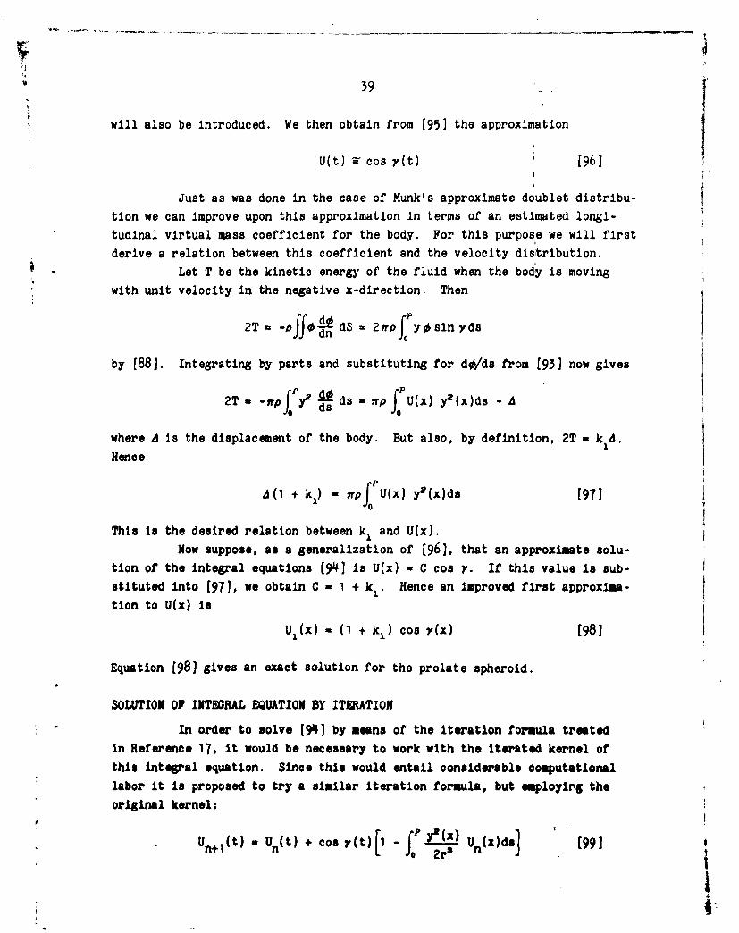
will also be introduced. We then obtain from [95] the approximation
U(t) 1 cos Y(t) [96]
Just as was done in the case of Munk's approximate doublet distribu-
tion we can improve upon this approximation in terms of an estimated longi-tudinal virtual mass coefficient for the body. For this purpose we will first
derive a relation between this coefficient and the velocity distribution.Let T be the kinetic energy of the fluid when the body Is moving
with unit velocity in the negative x-direction. Then
2T - -pffO It dS = 2rpjPy sinyds
by [88]. Integrating by parts and substituting for do/ds from [93] now gives
2T n -- rpf y2 A dsa rP, U(x) y2 (x)ds - A
where 4 is the displacement of the body. But also, by definition, 2T - k A.
Hence
A (1 +k) 7rpf U(x) y2(x)ds (97]
This is the desired relation between k and U(x).Now suppose, as a generalization of [96], that an approximate solu-
tion of the integral equations [941] is U(x) - C cos r. If this value is sub-stituted into [971, we obtain C - 1 + k1 . Hence an improved first approxima-tion to U(x) is
U,(x) - (1 + k) coB ,(x) (98]
Equation [981 gives an exact solution for the prolate spheroid.
SOLUTION OF INTEGRAL EQUATION BY ITERATION
In order to solve [941 by means of the iteration formula treatedin Reference 17, it would be necessary to work with the Iterated kernel ofthis integral equation. Since this would entail considerable computationallabor It is proposed to try a similar iteration formula, but employirg theoriginal kernel:
Un+ 1(t) - Un(t) + cos ,(t)[1- Jo 2 Un(x)ds] [99] I4.
40
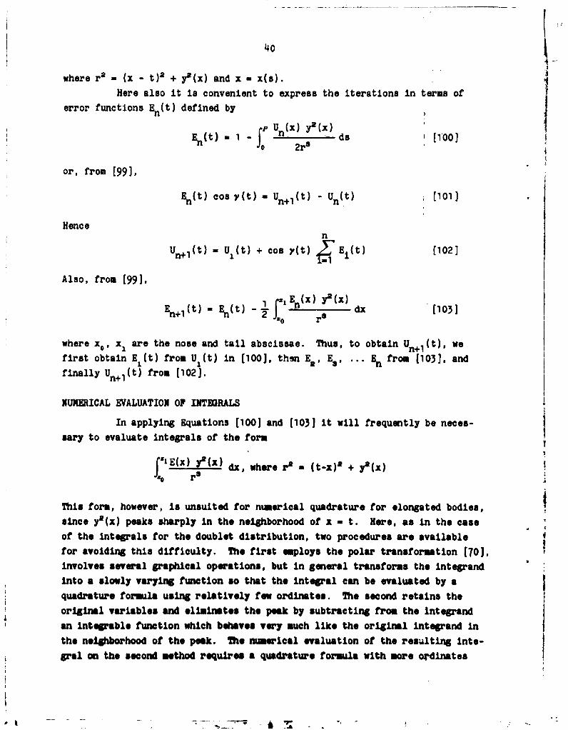
where ra - (x - t)2 + y2 (x) and x - x(s).
Here also it is convenient to express the iterations in terms oferror functions En(t) defined by
nUn X)En(t) 1 -1 ds 100fo 2r 3
or, from [99],
Eh(t) Cos 7(t) - Un+i(t) - Un(t) (101]
Henscen
l U (t) - I t) + Cos v(t) "E1 (t) (102]
Also, from (99],
En~(t) En(t) ziEn(x) y2 (x)ln12 r - dx [1031
o r=
where x0, x. are the nose and tail abscissae. Thus, to obtain Un+l(t), wefirst obtain ECt) from U,(t) in (100], then E., E3, ... En from (103], andfinally Un+l(t) from (102].
NUMERICAL EVALUATION OF INTEGRAL
In applying Equations (100] and [1031] it will frequently be neces-sary to evaluate Integrals of the form I
fE(x) l(x) dx, where 9 - l (t-x)2 + y9(x)
This form, however, is unsuited for numerical quadrature for elongated bodies,since e(x) peaks sharply In the neighborhood of x - t. Here, as In the caseof the integrals for the doublet distribution, two procedures are availablefor avoiding this difficulty. The first employs the polar transformation [70),involves several graphical operations, but In general transforms the integrandinto a slowly varying function so that the Integral can be evaluated by aquadrature formula using relatively few ordinates. The second retains theoriginal variables and eliminates the peak by subtracting from the integrandan integrable function which behaves very much like the original Integrand Inthe neighborhood of the peak. The numerical evaluation of the resulting inte-gpal on the second method requires a quadrature formula with more ordinates
4qm4,
than the first in order to obtain the same accuracy, but, since all graphical
operations are eliminated, the second method is suitable for processing on an
automatic-sequence calculating machine.
The result of the polar transformation has effectively been given
in [95]. We have,
f',E(x) Yl(x) dx E r E(x) sin' 2 jCoo (
Zo r3 sinjO-yx)] dO [104]
where
x - t - y(x) cot G (70]
It is desired to evaluate this integral for a series of values of t. In gen-
eral this can be done with sufficient accuracy by means of the Gauss 7- (or
11-) ordinate quadrature formulas. This gives 7 (or 11) values of 0 at which
the integrand needs to be determined for a given t. The value of x occurring
in the integrand is determined implicitly, for given values of t and 0, by the
polar transformation [70]. In practice the 7 (or 11) x's can be obtained
graphically from the intersections with a graph of the given profile of the 7(or 11) rays from the point x - t on the axis at the angles required by the
Gauss quadrature formula. If greater accuracy is desired, these graphicallydetermined values of x can be corrected by means of the formula
A
t-xg + y(x ) cot eX = Xg + - 9o15]
S+1-y'(xg) cot (15
in which xg is the graphically determined value and y' denotes the derivative
of y with respect to x.
Now let us derive an alternate, completely arithmetical procedure
for evaluating the integrals. Put
t ktxg(x, t)
k,(x, t) [(x-t) +
where yR = f(x) is the equation of the given profile and y, g(x, t) isthe equation of the prolate spheroid whose ends coincide with the ends of the
given body, and which intersects the given body at x = t. i.e.,-
*I s l '
42
g(x, t) - f(t) ([x1o)(x.)6](t-x0 )(xl t 16
The length-diameter ratio X of the spheroid is given by
(t-x.)(X-t)
f(t) [1071
whence the longitudinal virtual mass coefficient k (t) can be obtained from
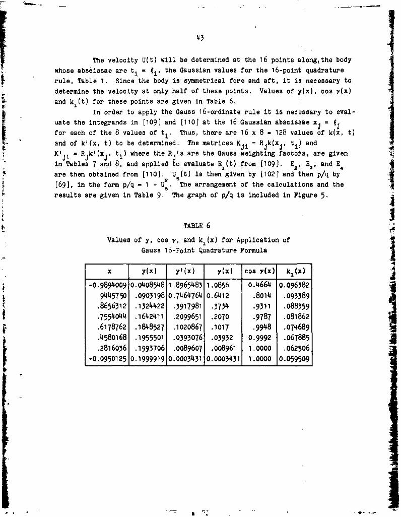
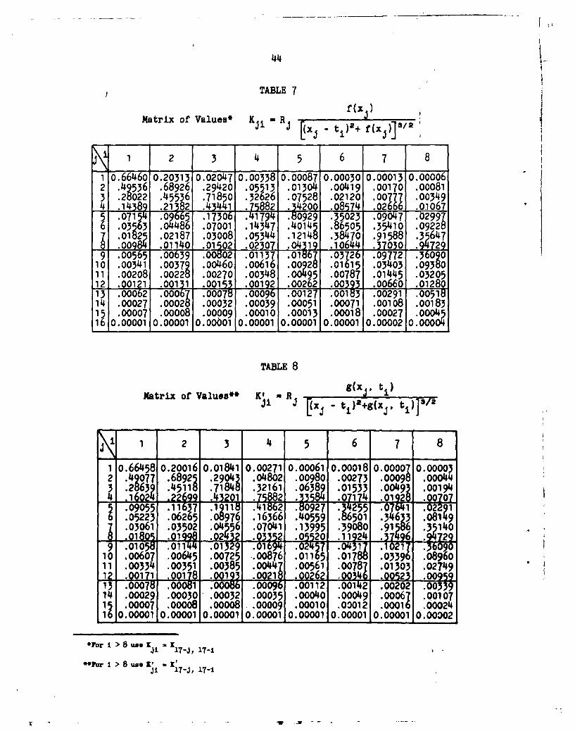
[26].Since U(x) - (1 + k.) cos Y(x) is an exact solution of [94] for the
prolate spheroid, we have
"k'(x t)dx [108]so
We now obtain, from [98], [100], and [108]+k 1 +k {o9
1 .k W .00 0. 1(' o l0000; 0a.00 0000 00% .00f--~~ 0 :35 +0(03 a 0029+.O"a+.06
FF
It +I (x9) o2T; 2 - .05
49
SUMMARY
Two new methods for computing the steady, irrotational, )axisymmetric
flow of a perfect, incompressible fluid about a body of revolution are
presented.
In the first method a continuous, axial distribution of doublets
which generates the prescribed body in a uniform stream is sought as a solu-
tion of the integral equation
fb m(t) dtrs
where r is the distance from a point (t, 0) on the axis to a point (x, y) on
the body, r2 a (x - t)2 + y2(x).
A method of determining the end points of the distribution and the
values of the distribution at the end points is given. If the equation of the
body profile, with the origin of coordinates at one end, is
y2(x) = aIx + a2x2 + a3x3 +
a very good approximation for the distribution limit a at that end, when the
coefficients a1 , a2P ... are small, is given by
a 4
a 2 2 1 3
if a. a 0. If as is negative, the term containing it is neglected. The cor-
responding value of the doublet strength at this point is
a a a
*~a -(P +;JL& + 2 log I a& V!7a
Por ualas and tables for determining a and r(a), which may be used when theabove procedure is insufficiently accurate, are also given. The values a, b,ma - a(s), a - m(b), fa - e(a) and fb - e(b) are then used to obtain theapproximate solution of the Integral equation
* .(x) -c " a'' f + s + .
I4!
I
,
50
where
l+kf" jy 2 dx (b'a)(m,+mb)
fy2dx -. b-a)Q(f)
and k is the longitudinal virtual mass coefficient for the body.
This approximation is used to obtain a sequence of, successive approx-
imations by means of the iteration formula
m+(x) M (x) +_1 y2(X) ) 1 dtmi+1 m 2 L2
0 r5 -
When a doublet distribution has been assumed, the velocity components at a
point (x, y) in a meridian plane are
bt-
U + f b(-L .Z L m(t)dt~~5 3
v - 3yf -- m(t)dtrs
and the pressure is. given by
-1-. (u + V)q
where q is the stagnation pressure.
The iterations are most conveniently performed in terms of the dif-
ferences between successive approximations to r(x), which also furnish, at
each iteration, a geometric measure of the accuracy of an approximation. )Simpler forms for the velocity components at the surface of the body are given
in terms of this difference or error function.
Gauss' quadrature formulas are recommended for the numerical eval-
uation of the integrals. Two methods of carrying out the iterations are
given. The first employs a polar transformation and a graphical operation be-
tween successive iterations; the second is completely arithmetical and is
suitable for processing on an automatic-sequence computing machine. All of
these procedures are illustrated in detail by an example, in which the semi-
graphical method Is employed. The accuracy of the method is ana'lyzed; the re-
suits are compared with those obtained by the methods of JruK n and Kaplan.
51
In the second method the velocity U(x) on the surface of the given
body Is given directly as the solution of the integral equation
f U(x)y'(x) ds = 10' 2r3
where s is the arc length along the profile,
x is equal to x(s), and
2P is the perimeter of a meridian section.
An approximate solution to this integral equation is
U (x) = (1 + k) cos y(x)
where k is the longitudinal virtual mass coefficient and y = arctan d
U1(x) is used to obtain a sequence of successive approximations by means of
the iteration formula
Un+1(t) - Un(t) + cos V(t)[1 - a(x) Un(Xds]
Here, also, the Iterations are most conveniently carried out in terms of the
differences between successive approximations to U(x) which also furnish a
measure of the error in the integral equation. Two methods of carrying out
the iterations are again available, of which one is semi-graphical, the other
completely arithmetical. The latter technique is employed on the same example
as was used to illustrate the first method.
j I• I
52
APPENDIX
END POINTS OF A DISTRIBUTION
An approximate method for determining the end points of a distribu-
tion and its trends at the ends will now be described. Let y - f(x) be the
equation of the given profile extending from x - 0 to x - 1; let m(x) be the
corresponding doublet distribution, extending from x - a to x - b., It will be
assumed that 0 < a << b < 1 and that a is near 0, b is near 1. Then m(x) is
given by the integral equation
bf m(tidt [1 ]]
[(x-t)2 + f(x)] 1/' 2 4
Various conditions on m(x) may now be obtained by differentiating j[111 repeatedly with respect to x. We get
f mlt)[2x - 2t + f'l(x)] dt - 0 [1121"r
JMMtL~ (2x - 2t + -') (J2 + t 0 [13I
m, MM5(2x-2t+f 1 )3 15 (2+f")( t+f) +- - r Jdt - 0 [1141
When x- 0, r = t and, writing f(x) as a Taylor expansion sa
(x) - a x + a x2 + a x3 + ... [1151
then also f'(0) - a, f"(O) - 2a , f'" (0) - 6a . Now, setting x = 0 In Equa- -
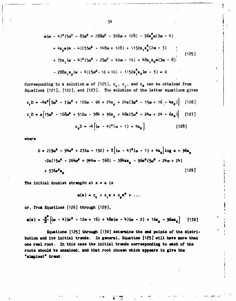
Corresponding to a solution a of [125], co, c1, and c2 can be obtained fromEquations [121], [122], and [123]. The solution of the latter equations gives
Equations (125] through [130] determine the end points of the distri-
bution and Its Initial trends. In general, Equation [125] will have more thanone real root. In this case the initial trends corresponding to each of theroots should be examined, and that root chosen which appears to give the
"simplest" trend.
7-1
55
The equations can be solved explicitly in the case of a very elon-
gated body for which a1, a2 , as .... in [1151 are all very small. First let
us suppose that they are so small that all the terms in [125] containing them
are negligible, so that the first product term alone may be equ4ted to zero,i.e.,