TWO-DIMENSIONAL DOMAINS RELATED. (U) INSTITUTE FOR COMPUTER APPLICATIONS IN SCIENCE AND ENGINEERIN, UNCLASSIFIED H T BANKS ET AL MAR 88 ICASE-88-23 F/G it/4 UL E E E E E E E E EEEII I I OL I N EEEEEEEEEEEEEE Em.....IIII
Transcript
TWO-DIMENSIONAL DOMAINS RELATED. (U) INSTITUTE FORCOMPUTER APPLICATIONS IN SCIENCE AND ENGINEERIN,
UNCLASSIFIED H T BANKS ET AL MAR 88 ICASE-88-23 F/G it/4 UL
E E E E E E E E EEEII I I OL I N
EEEEEEEEEEEEEEEm.....IIII
,
' KS
,3
10-0Upz
1 2 1111 , .4 .,l
BHI~:
NASA Cotaco Report 1864fiLt
ICASE REPORT NO. 88-23 .
0
ICASE-~ ~ BOUNDARY SHAPE IDENTIFICATION PROBLEMS
IN TWO-DIMENSIONAL DOMAINS RELATED TO
- THERMAL TESTING OF MATERIALS
DTICSELECTE*JUN07 I
* H. T. Banks
Fumio Kojima cb
DS
Contract No. NASI-18107 A~~a o ulMarch 1988 DVfiu' crlcqZ
%4 . .%j a
* INSTITUTE FOR COMPUTER APPLICATIONS IN SCIENCE AND ENGINEERINGNASA Langley Research Center, Hampton, Virginia 23665
Operated by the Universities Space Research Association N
* National Aeronautics andSpace AdministrationLangle Reswich CmitwHampton, Virginia 23665
%4
BOUNDARY SHAPE IDENTIFICATION PROBLEMS IN UTWO-DIMENSIONAL DOMAINS RELATED TO THERMAL
TESTING OF MATERIALS
H. T. BanksCenter for Control Sciences
Division of Applied Mathematics
Brown UniversityProvidence, RI 02912
Fumio KojimaInstitute for Computer Applications in Science and Engineering r,"
NASA Langley Research CenterHampton, VA 23665
%
Abstract
This paper is concerned with the identification of the geometrical structure of thesystem boundary for a two-dimensional diffusion system. The domain identificationproblem treated here is converted into an optimization problem based on a fit-to-data 0
criterion and theoretical convergence results for approximate identification techniquesare discussed. Results of numerical experiments to demonstrate the efficacy of thetheoretical ideas are reported.
;o,'t;.le io%o, ) DC op
'IV 0
__ I _ _ _
This research was supported by the National Aeronautics and Space Administration under NASA Con-tract No. NASI-18107 while the authors were in residence at the Insitute for Computer Applications in
Science and Engineering (ICASE), NASA Langley Research Center, Hampton, VA 23665. Also, researchwas supported for the first author in part by the National Science Foundation und r NSF Grant No. MCS-8504316, by the Air Force Office of Scientific Research under contract F49620 -C-011, and the National
Aeronautics and Space Administration under NASA Grant No. NAG-I-517.
%
I. INTRODUCTION
Domain identification problems are important in the design of engineering systems and
frequently such problems are treated as a branch of the calculus of variations which involves
nonlinear optimization techniques, optimal control theory, partial differential equations (el-
liptic, parabolic, hyperbolic, etc.) and related numerical methods. Domain identification
for elliptic systems has been studied theoretically and numerically by many authors (see
e.g., [5],[7],[10],[13]). For parabolic systems, a couple of numerical methods for identi-
fying the domain or boundary have been investigated.in [14],[151. . Until recently, most
investigations concentrated on the "optimal shape design problem" which is motivated by
numerous applications to structural, engine, airplane, ship designs, etc. (see [10] and the _
references therein).'In this paper, our concern for domain identification is motivated by an
application that is different from these shape design problems. However, as we shall see, .5
the resulting theoretical aspects are closely related. Recently, associated with the use of
fiber reinforced composite materials for aerospace structures, there is growing interest in
the detection and characterization of large structural flaws which may not be detectable
by visual inspection. One recent effort has focused on non-destructive evaluation methods
(NDE) based on the measurement of thermal diffusivity in composite materials (see e.g.,
(8]). Motivated by these problems, we consider the domain identification for parabolic
systems..
To explain our approach, we restrict our attention to a 2-D domain identification prob-
lem. We consider the bounded domain G(q) in two-dimensional Euclidean space as follows:
where x, -* r(xl, q) is some parameterized real function which is assumed to characterize
the unknown part of the boundary and q is a constant parameterization vector to be
identified among values in a given compact admissible parameter set Q. As depicted in
'46 Aw' 5-, .5 -
1.2 ,acq X2=r(x1,q )
1.0 .
0.8
ac 4 dC 2
0.4 - G(q)
0.2
O0I ac 1 I
0.00.0 0.4 0.8 1.2
Fig. 1.1. The spatial domain G and its boundary aGI, aG 2, 4G., 8G 4.
Fig. 1.1, we assume the boundary of G(q) consists of the following components:
aG, = {X = (I,, 2 )o < X, < 1, X2 = 0}
a2 a = {X = (XI,X2)Iz, = 1, 0 < X2 < t}
aq = X = (X,X2)o < I<1, X2 = r(XI,q)}
aC4 = {X = (X,X2)IX = 0, 0 < X2 <
The measurement system is described by the following 2-D diffusion equation:
e...', au (t, x) '8u"t ,z) Au(t,x) + cou(t, x) = 0 in T x G(q) (1.a)at
with the initial and boundary conditions,
u(0,x) = fro(x) on G(q) (1.1b)
2
z 5 M -
+ (, )=o on T'x OG, (1.1c)u
c 1 -± + hu =- on T x aG 2 (1.1d)ax2auc- 0 on Txacq (1.1e)-c x 1 h = T, (1 .1 d )
au
aC5- u =0 on T x OG4 (.f
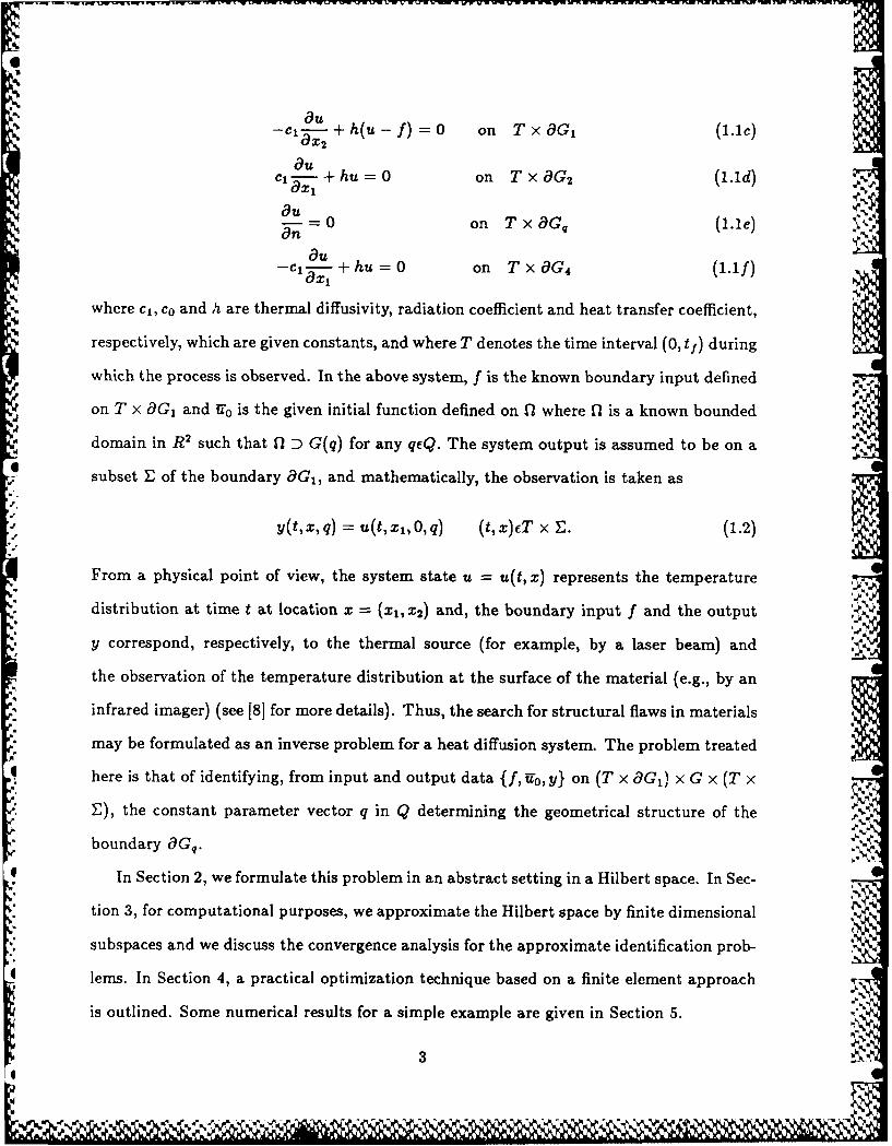
where cl, co and h are thermal diffusivity, radiation coefficient and heat transfer coefficient,
respectively, which are given constants, and where T denotes the time interval (0, tf) during
which the process is observed. In the above system, f is the known boundary input defined V
on T x aG 1 and U0 is the given initial function defined on 12 where 11 is a known bounded
domain in R2 such that fl D G(q) for any qEQ. The system output is assumed to be on a
subset E of the boundary aG 1 , and mathematically, the observation is taken as
y(t,x,q) = u(t,xj,0,q) (t,x)ET x E. (1.2)
From a physical point of view, the system state u = u(t,x) represents the temperature
distribution at time t at location x = (X1 , X2) and, the boundary input f and the output
y correspond, respectively, to the thermal source (for example, by a laser beam) and
the observation of the temperature distribution at the surface of the material (e.g., by an
infrared imager) (see [8] for more details). Thus, the search for structural flaws in materials
may be formulated as an inverse problem for a heat diffusion system. The problem treated
here is that of identifying, from input and output data {f, 0 y} on (T x xG) x G x (T x
E), the constant parameter vector q in Q determining the geometrical structure of the
boundary 8 Gq.
In Section 2, we formulate this problem in an abstract setting in a Hilbert space. In Sec-
tion 3, for computational purposes, we approximate the Hilbert space by finite dimensional N
subspaces and we discuss the convergence analysis for the approximate identification prob-
lems. In Section 4, a practical optimization technique based on a finite element approach
is outlined. Some numerical results for a simple example are given in Section 5.
where a* (q)(.,.) is the adjoint sesquilinear form of a(q)(.,.) defined by
.t.h
+ [OV)adz. + I flkpV)IGuG, Z2
:.f: ro, z1)(¢ f1
+ flr'(qIq, z1) r (q, z) - 1[uizkaG¢dzz
1 ,q[ , dz). f [001acdzi.A. r (q, zi)
Consequently, the optimality condition (4.1) of the problem (AIDP)N can be characterized
by -
n
t vN(t, N)l{[VqkAN( N)]wN(t, N)- VqN(t,F N)}(q - 4kN) > 0 for all q6Q.
(4.4)
In the sequel, we discuss computer implementation of numerical schemes for the prob-
lem (AIDP)N. Since we can evaluate the gradient of the cost function using (4.2), many
* optimization techniques for the constrained problems are readily applicable to our problem
(see [11] and the references therein). For ease in exposition, here the compact set Q C RN "
is assumed to be defined by
Q = {q (q, 2, q,...,,)cRNq < i (4.5)
where fl and i denote a given constraint matrix and vector, respectively. For the numer-
%%N
• .'. 15
a particularly useful technique for optimization problems with the linear inequality con-
straints such as those given in (4.5). We use this method as presented in [12]; the iterative
algorithm for finding ,N can thus be stated as follows:
_* Step 0: Choose an initial value q(0) in Q and set i = 0.
Step 1: If flq(4) < -q set
g(i) = _VqjN(q('))
and proceed to Step 3; otherwise, proceed to Step 2.
Step 2: Compute the current direction by
PV J N (()), g(I) = PqjN~q ( )
9 "pVqJN(q(i))l
W .. where
T-1,(Ilprl,) - ipP =1
and rip includes the gradient of all currently active constraints associated with matrix H.
If g(') =f 0, proceed to Step 3; otherwise, proceed to Step 4.
Step 9: Compute \(.n satisfying
jNi~~~() mi N( + Ag(')
J q(') + ,2ngC)) m J= (q)
where . is the largest step that may be taken from q(') along g(') without violating any
constraint. If A = A, then add the new contraints to the matrix TIP and proceed to Step
4; otherwise, the new approximation to the solution is given by
q(i+l) = q(i) + A(ng().0I
Replace i + 1 by i and return to Step 1.
Step 4: Compute the vector O(q) by
.... "O(q(i)) = ( ~prj')-lIpVpJ(q(i)).
16
• i
PL- - IV -L x,- PL W, IC T IL.. W177V - a,- .'L Rn 'L n" K NO W .' ECT I .T ' N] iU ~JW I AR WRLRRVJS -~LR IL V -~,~
If all components of 0 are nonnegative, then set
' = q(t)
and terminate the computation; otherwise, delete the column of IH, corresponding to the
smallest component of (q(')), replace i + 1 by i and return to Step 1.
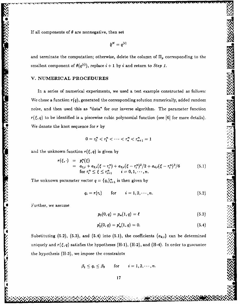
V. NUMERICAL PROCEDURES
In a series of numerical experiments, we used a test example constructed as follows:
We chose a function r(q), generated the corresponding solution numerically, added random
noise, and then used this as "data" for our inverse algorithm. The parameter function
r( , q) to be identified is a piecewise cubic polynomial function (see [6] for more details).
* We denote the knot sequence for r by
_ 0= o < T <" n< T n+ =
and the unknown function r( , q) is given by
p.. .**
= a, + a2,i( - Fin) + a 3.,(e - rtl)2/2 + a 4,i(e - r,")3/6 (5.1), ' . ~ ~~~for rin < e <! rin, i=0,1..n -
The unknown parameter vector q {qi}!= is then given by
q= r(ri) for i =1,2,.--,n. (5.2)
* further, we assume
.. "~p 0O, q) p. p,(1, q) = (5.3)-.""
p0'(O,q) = p'(1,q) = 0. (5.4)
- Substituting (5.2), (5.3), and (5.4) into (5.1), the coefficients {ak,i} can be determined
uniquely and r(e, q) satisfies the hypotheses (H-I), (H-2), and (H-4). In order to guarantee
the hypothesis (11-3), we impose the constraints
3 < q; -< #2 for i=1,2, .- ,n.
17
I.%
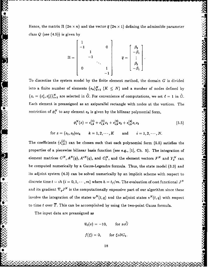
-Hence, the matrix I1 (2n x n) and the vector (2n x 1) defining the admissible parameter
class Q (see (4.5)) is given by
-0 )32
11 P20 1 L -01~ J
To discretize the system model by the finite element method, the domain G is divided
into a finite number of elements {ek}_ (K < N) and a number of nodes defined by
= 2, z)i=1 are selected in G. For convenience of computations, we set t = 1 in c.Each element is preassigned as an axiparallel rectangle with nodes at the vertices. The
restriction of Of' to any element ek is given by the bilinear polynomial form,
N(Z) = +.el ) + C c,(,. (5.5)
forz= (z1,z2 )Eek k=1,2,...,K and i=1,2,..-,N.
The coefficients {c(.j} can be chosen such that each polynomial form (5.5) satisfies the
properties of a piecewise bilinear basis function (see e.g., [1], Ch. 5). The integration of
element matrices CN, AN(q), A*N(q), and CN, and the element vectors FN and Yd can
be computed numerically by a Gauss-Legendre formula. Thus, the state model (3.3) and
its adjoint system (4.3) can be solved numerically by an implicit scheme with respect to
discrete time t = ih (i = 0, 1,.., m) where h = t/m. The evaluation of cost functional jN
and its gradient Vq jN is the computationally expensive part of our algorithm since these
involve the integration of the states wN(t, q) and the adjoint states vN(t, q) with respect
OF, to time t over T. This can be accomplished by using the two-point Gauss formula.
The input data are preassigned as
" 0(z) = -10, for zcG
f( ) 0, for caG1 .
18
a6.
"?.". Tihe known parameters cl, co, and h in Eq. (1.1) were set as .
c, 0.034, c2 0.001, h =0.1.
""'" The observed data {yd(t)} were generated by solving the finite element model (3.3). The.-
number of finite elements and nodes in the numerical experiments were set as K =256 =,
,., 16 x 16) and N = 289 (= 17 x 17), respectively. The final time and number of time
d .'.divisions were taken as tf = 10 and m = 100. Random noise at various levels from 0% to
~50'c was added to the numerical solution, thereby producing simulated noisy "data" for
~~the algorithm. The set E relative to data acquisition was given by .
I U N.,
where N denotes a neighborhood of points at G , i.e.,
.N, = (x i - , x c + ) for 1 21. p.
Using such data, the estimation algorithm given in Section 4 was tested.
Example 1: In this example, the dimension of unknown vector was taken as n 4 and the
knot hm.uhe s re vo t q i was given by " Sn
,r-4 = i /5 for i =1,2,...,5.
.51
wThe value deotte aamneghb ro ofr pon atsC, ~.
-'
• fl 2 1.1, respectively. The initial guesses for the parameters were given by ,.
5,
q(0) = 1 for i = 1,2,3,4. ,p
The number of sensors was taken as p 9. Table 1 shows the estimated parameter numer-ical results for the data with noise free, 5%, 10%, and 50% relative noise and Figure 5.1
19 q
S e4:..-V
• '.5>
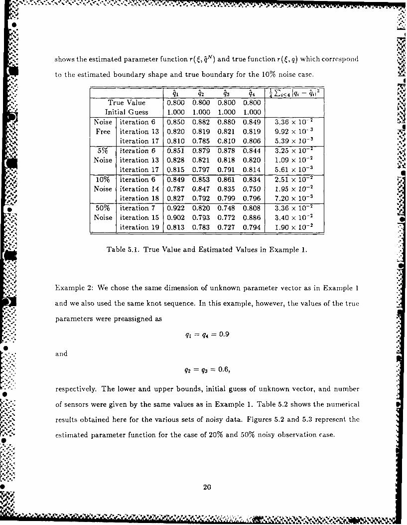
"5 shows the estimated parameter function r(, 4N) and true function r(E, q) which correspond
to the estimated boundary shape and true boundary for the 10% noise case.
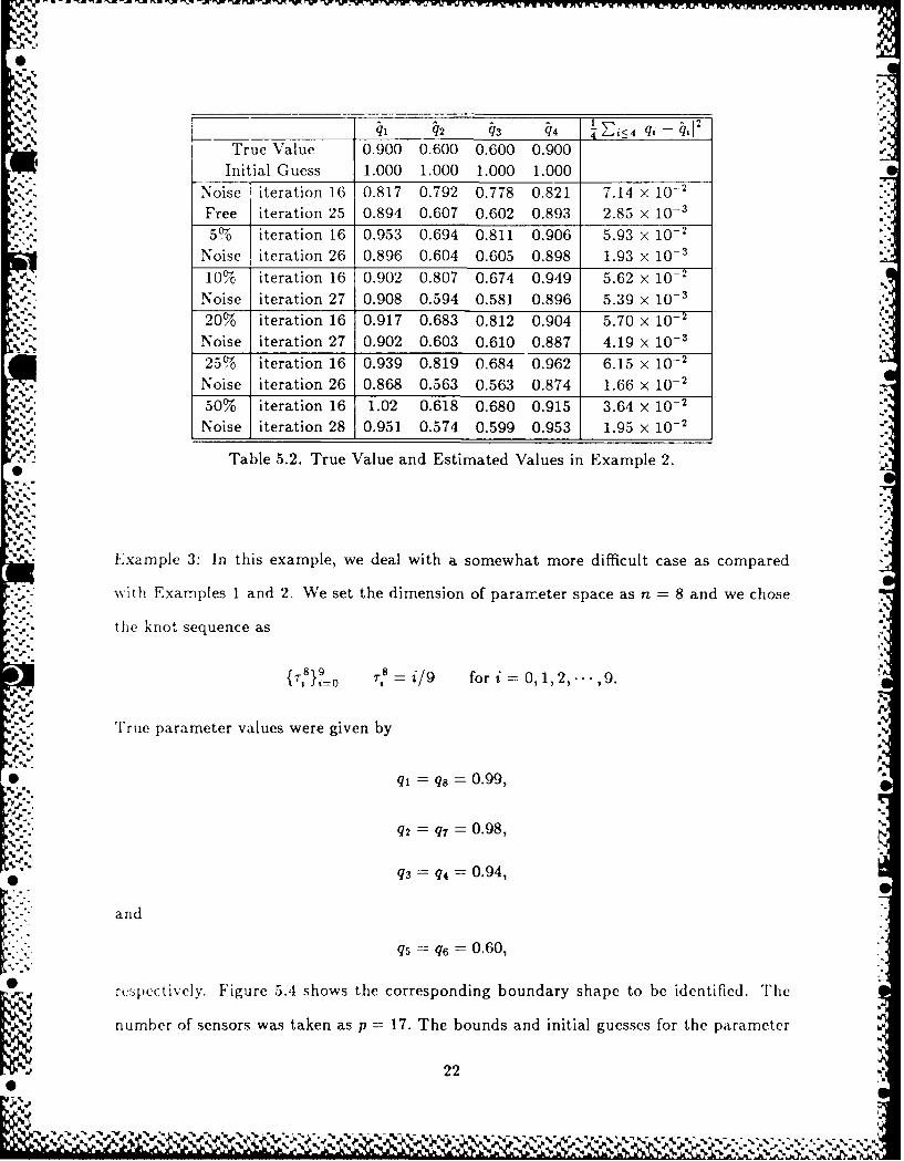
41 42 43 4 j1 i :5,4 jqj - 4i,' OTrue Value 0.800 0.800 0.800 0.800
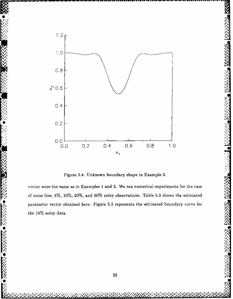
Table 5.3. True Value and Estimated Values in Example 3.
* Throughout the numerical experiments, we checked the robustness of the algorithm with
respect to noise in the observed data. Results in three examples indicated that the algo-
rithm worked very well (i.e., as expected) for various noise levels. Furthermore, we checked
the sensitivity of the algorithm with respect to the number of sensors. Specifically, we com-
pared in Examples 2 and 3 the number of sensors (p) with the dimension of parameter
spae n).InExample 2, for data with p=5(> n=4), the algorithm still yields an almost
identical fit (to that for p = 9) even in 50% noise case while the fit could not be achieved
under the reduced observation case p = 3(< n). Also, in Example 3, (where n =8) the
F-fit could not be obtained with p =3 or p =5, while the algorithm performed well with
* p = 9 (> n). Carrying out a large number of other numerical tests in addition to those
reported for Examples 2 and 3, we suggest that the algorithm requires a number of sensors
which is at least equal to the number of dimensions of parameter space, i.e., p > n. '
VI. CONCLUDING REMARKS
In this paper, we have discussed techniques for estimating the system boundary shape
* in two dimensional parabolic systems. By using a simple coordinate transformation tech-a
nique, the parabolic PDE defined on unknown spatially varying domain was converted%
26
-.- )
1 .0 -- -- - -- - -- - -- - -- - -- -
0.8
= x 0.6 -
0.4 True Function
Initial Guess
0.2 Estimated Function
0.0.0.0 I I I
0.0 0.2 0.4 0.6 0.8 1.0
S .4%_
Figure 5.5. True Function and Estimated Function in Example 3 (10% Noise).S
.. 1*
27
S* % . %,
into the same type PDE with unknown coefficients defined on a fixed domain. Thus, our
fundamental approach was placed within the theoretical framework for parameter identifi-
cation problems given in [21,[3], and [4]. The practical utility of our algorithm is supported
N. through a series of numerical experiments, a summary of which is given in Section 5. These
simulations were carried out on the Sun Microsystems at ICASE, NASA Langley Research
%* Center. For three different numerical examples, using data with no noise, the proposed '
algorithm yields an almost perfect fit, while, as expected, the fit degenerates significantly
as noise in the observation becomes more pronounced.
Although here we discuss only the case where the unknown boundary shape is rep-
resented by a simple function of one variable, our basic parameter estimation ideas andtechniques can be readily extended to consider more general classes of geometrical struc-
tures for the system boundary. For example, we may also treat the case where the unknown
boundary shape is characterized by '
r(q,X1, X2 ) =0 for (X1, X2 ) ER'.
We are currently pursuing investigations for these cases.
ACKNOWLEDGEMENT
'p The authors would like to express their sincere appreciation to Dr. W. Winfree and
Ms. Michele Heath (Instrument Research Division - Materials Characterization Instru-
mentation Section, NASA Langley Research Center) for numerous conversations and en-
couragement during the course of this research. Their suggestions and questions were anS essential motivation of our efforts.
00
28
0V
References
[1] 0. Axelsson and V. A. Barker, Finite Element Solution of Boundary Value Problems,
Academic Press, New York, 1984.
N [2] H. T. Banks, "On a variational approach to some parameter estimation problems,"
Distributed Parameter Systems, Lecture Notes in Control and Information Sciences,
Vol. 75 (1985), pp. 1-23, Springer-Verlag, New York.
[3] H. T. Banks and K. Ito, "A theoretical framework for convergence and continuous
dependence of estimates in inverse problems for distributed parameter systems,"
LCDS/CCS Report No. 87-20, Brown University, March 1987; Appl. Math. Lett.,
• Vol. 0 (1987), pp. 31-35.
[4] H. T. Banks and K. Ito, "A unified framework for approximation in inverese problems
-for distributed parameter systems," LCDS/CCS Report No. 87-42, Brown University,
October 1987; Control Theory Adv. Tech., to appear.
[5] D. Begis and R. Glowinski, "Application of the finite element method to the ap-proximation of an optimum design problem," Appl. Math. Optim., Vol. 2 (1975), pp.
130-168.
. [6] C. de Boor, A Practical Guide to Splines, Applied Mathematical Science, Vol. 27,
0 Springer-Verlag, New York, 1978.
[7] D. Chenais, "On the existence of a solution in a domain identification problem,"
J. Math. Anal. Appl., Vol. 52 (1975), pp. 189-219.
[8] D. M. Heath, C. S. Welch, and W. P. Winfree, "Quantitative thermal diffusivity -'
measurements of composites," in Review of Progress in Quantitative Nondestructive
* Evaluation, (D. G. Thompson and D. E. Chimenti, eds.), Plenum Publ., Vol. 5B
(1986), pp. 1125-1132.
29
ne-
. ! ~
9' J. L. Lions, Optimal Control of Systems Governed by Partial Differential Equations,
Springer-Verlag, New York, 1971.
10' 0. Pironneau, Optimal Shape Design for Elliptic Systems, Springer-Verlag, New .
York, 1983.
J111 E. Polak, Computational Methods in Optimization, Academic Press, New York, 1971.
12' J. B. Rosen, "The gradient projection method for nonlinear programming, Part I:
Linear constraints," SIAM J. Appl. Math., Vol. 8 (1960), pp. 181-217.
13] J. Simon, "Differentiation with respect to the domain in boundary value problems,"
- Numer. Funct. Anal. Appl., Vol. 2 (1980), pp. 649-687.
141 Y. Sunahara, Sh. Aihara, and F. Kojima, "A method for spatial do- -
main identification of distributed parameter systems under noisy observations,
Proc. 9th IFAC World Congress, Budapest, Hungary, 1984, Pergamon Press, New
-" ' York, 1984.
15' Y. Sunahara and F. Kojima, "Boundary identification for a two dimensional diffu-
sion system under noisy observations," Proc. 4th IFAC Symp. Control of DistributedParameter Systems, UCLA, California, 1986, Pergamon Press, New York, 1986.
% 30
L:--V
.'- J.V
300:
::,-.. -
l - ... II| H HO~U Nn | an l~d tld a hm m dU n U-' V.
..
*
* IftIAEjA,
Report Documentation Pg
i1 Report No 2 Government Accession No 3 Recipient's Catalog No
-,NASA CR-181654 r-7
I..,.. CASEReport No. 88-23 - __"___- __- T epr
4 Title and Subtitle 5 Report Date
BOUNDARY SHAPE IDENTIFICATION PROBLEMS IN TWO- March 1988.. DIMENSIONAL DOMAINS RELATED TO THERMAL TESTING 6 r
OF MATERIALS 6 Performing Organization Code
7 Authorls) 8. Performing Organization Report No
H. T. Banks and Fumio Kojima 88-23 10
10. Work Unit No.
9 Performing Organization Name and Address
Institute for Computer Applications in Science 11. Contractor Grant No.
and Engineering NASI-18107Mail Stop 132C, NASA Langley Research Center
* L ~ nn A 9A £ 9 13. Type of Report and Period Covered
National Aeronautics and Space Administration.;..- angey eserchCener14. Sponsoring Agency Code* Langley Research Center
Hampton, VA 23665-5225
15, Supplementary Notes
Langley Technical Monitor: Submitted to Quart. Applied Math.
Richard W. Barnwell
Final Report
16. Abstract
This paper is concerned with the identification of the geometrical structureof the system boundary for a two-dimensional diffusion system. The domainidentification problem treated here is converted into an optimization problem
based on a fit-to-data criterion and thaorketical convergence results forapproximate identification techniques are discussed. Results of numerical
*experiments to demonstrate the efficacy of the theoretical ideas are reported.
% : 17 Key Words (Suggested by Authorls)) 18 Distribution Statement)9 - Mathetmatical and Computt,r Sci( n s
[ .' parameter estimation, distributed ((4-n (-,ra 1)"""parameter systems, parabolic systems 64 - N ume r icaI A naI\'.s is
~domain identification h-SsesAayi
• [lm'a~sifid - un imite'd
.%/. -,..19 Security Classf (ofth~s report) 20 Security Classif (ofthos page, 1'2 No of pages 22 Price
%',r Unclassified Unclassified 32 A0)3- %w. ; ASA FORM 162 OCT 96