UNCORRECTED PROOFS - Department of Mathematics - University

OPTIMAL CONTROL APPLICATIONS AND METHODSOptim. Control Appl. Meth. (2008)Published online in Wiley InterScience (www.interscience.wiley.com). DOI: 10.1002/oca.855

The role of symplectic integrators in optimal control

Monique Chyba1,∗,†, Ernst Hairer2 and Gilles Vilmart2,3

1Department of Mathematics, University of Hawaii, 2565 Mc Carthy the Mall, Honolulu 96822, HI, U.S.A.2Section de Mathematiques, Universite de Geneve, 2-4 rue du Lievre, CH-1211 Geneve 4, Switzerland

3INRIA Rennes, ENS Cachan Antenne de Bretagne, Avenue Robert Schumann, 35170 Bruz, France

SUMMARY

For general optimal control problems, Pontryagin’s maximum principle gives necessary optimality condi-tions, which are in the form of a Hamiltonian differential equation. For its numerical integration, symplecticmethods are a natural choice. This article investigates to which extent the excellent performance ofsymplectic integrators for long-time integrations in astronomy and molecular dynamics carries over toproblems in optimal control.

Numerical experiments supported by a backward error analysis show that for problems in low dimensionclose to a critical value of the Hamiltonian, symplectic integrators have a clear advantage. This is illustratedusing the Martinet case in sub-Riemannian geometry. For problems like the orbital transfer of a spacecraftor the control of a submerged rigid body, such an advantage cannot be observed. The Hamiltonian systemis a boundary value problem and the time interval is in general not large enough so that symplecticintegrators could benefit from their structure preservation of the flow. Copyright q 2008 John Wiley &Sons, Ltd.

Received 17 January 2008; Revised 14 April 2008; Accepted 25 April 2008

KEY WORDS: symplectic integrator; backward error analysis; sub-Riemannian geometry; Martinet;abnormal geodesic; orbital transfer; submerged rigid body

1. INTRODUCTION

For the numerical solution of optimal control problems, there are essentially two approaches: thedirect approach, which consists in discretizing the problem directly and applying optimizationtechniques, and the so-called indirect approach, which is based on Pontryagin’s maximum principle.The maximum principle provides necessary conditions that reduce the optimal control problem

∗Correspondence to: Monique Chyba, Department of Mathematics, University of Hawaii, 2565 Mc Carthy the Mall,Honolulu 96822, HI, U.S.A.

†E-mail: [email protected]

Contract/grant sponsor: Fonds National Suisse; contract/grant number: 200020-109158Contract/grant sponsor: National Science Foundation; contract/grant number: DMS-030641

Copyright q 2008 John Wiley & Sons, Ltd.

UNCORRECTED PROOFS

M. CHYBA, E. HAIRER AND G. VILMART

to a system of Hamiltonian differential equations with boundary conditions, which can be solvedusing shooting techniques. The present article is concerned with the indirect approach.

There are many arguments in favor of using symplectic integrators for the numerical solu-tion of the Hamiltonian system. Firstly, geometric numerical integration [1] puts forward the useof structure-preserving algorithms for the solution of structured problems such as Hamiltoniansystems. This is justified by a backward error analysis that allows one to interpret the numer-ical solution of a symplectic method as the exact flow of a modified Hamiltonian system. Thisexplains the excellent long-time behavior of such integrators. Furthermore, a series of papers [2–5]develops variational integrators for optimal control problems and emphasizes their symplecticity.The work of Hager [6] and Bonnans and Laurent-Varin [6, 7] shows that for partitioned Runge–Kutta discretizations based on symplectic pairs, the direct and indirect approaches are equivalent.

On the other hand, the Hamiltonian systems arising in optimal control are quite different fromthose in astronomy and molecular dynamics, where symplectic integrators have proven to be themethod of choice. Pontryagin’s maximum principle yields a boundary value problem and long-timeintegration is in general not an issue. Furthermore, the modified Hamiltonian system (in the senseof backward error analysis) is not necessarily a differential equation that arises from a modifiedoptimal control problem. It is therefore not obvious whether symplectic integrators will be superiorto standard methods. The aim of this article is to study this question and to investigate the practicaleffect of using symplectic integrators in the numerical solution of optimal control problems. Thiswill be done in several case studies.

For problems in low dimension, which are close to a critical value of the Hamiltonian, symplecticintegrators turn out to have a significant advantage. This happens for the so-called Martinet casein sub-Riemannian geometry, see [8, 9] and the references therein. The Martinet flat case and anon-integrable perturbation are introduced in Section 2 together with the corresponding differentialequations. Numerical experiments with an explicit Runge–Kutta method and with the symplecticStormer–Verlet method are presented in Section 3 and illustrated with figures. Close to abnormalgeodesics, the results are quite spectacular. For a relatively large step size, the symplectic integratorprovides a solution with the correct qualitative behavior and a satisfactory accuracy, while forthe same step size the non-symplectic integrator gives a completely wrong numerical solution,particularly for the non-integrable case. The explanation relies on the theory of backward erroranalysis (Section 4).

Unfortunately, this explanation cannot be extended to general optimal control problems. Wepresent two examples: the orbital transfer of a spacecraft (Section 5) and the control of a submergedrigid body (Section 6). The Hamiltonian system for the submerged rigid body is very sensitivewhen considered as an initial value problem and thus requires the use of multiple shooting tosolve the boundary value problem. For both problems, symplectic integrators do not show any realadvantage. The reason is that the time interval is not long enough so that the symplectic integratorcould benefit from structure preservation.

2. A MARTINET-TYPE SUB-RIEMANNIAN STRUCTURE

Let (U,�,g) be a sub-Riemannian structure, where U is an open neighborhood of R3, � adistribution of constant rank 2 and g a Riemannian metric. When � is a contact distribution, thereare no abnormal geodesics, and a non-symplectic integrator is as efficient as a symplectic one.However, when the distribution is taken as the kernel of the Martinet one-form, we show that

Copyright q 2008 John Wiley & Sons, Ltd. Optim. Control Appl. Meth. (2008)DOI: 10.1002/oca

UNCORRECTED PROOFS

THE ROLE OF SYMPLECTIC INTEGRATORS IN OPTIMAL CONTROL

a symplectic integrator is much more efficient for the computation of the normal geodesics andtheir conjugate points near the abnormal directions.

We briefly recall some results of Agrachev et al. [8] for a sub-Riemannian structure (U,�,g).Here, U is an open neighborhood of the origin in R3 with coordinates q= (x, y, z), and g isa Riemannian metric for which a graduated normal form, at order 0, is g= (1+�y)dx2+(1+�x+�y)dy2. The distribution � is generated by the two vector fields F1=�/�x+(y2/2)�/�z andF2=�/�y, which correspond to �=ker�, where �=dz−(y2/2)dx is the Martinet canonicalone-form. To this distribution we associate the affine control system

q=u1(t)F1(q)+u2(t)F2(q)

where u1(t),u2(t) are measurable bounded functions that act as controls.We consider two cases, the Martinet flat case g=dx2+dy2, an integrable situation, and a one-

parameter perturbation g=dx2+(1+�x)2dy2 for which the set of geodesics is non-integrable.

2.1. Geodesics

It follows from the Pontryagin maximum principle, see [8, 9], that the normal geodesics corre-sponding to g=dx2+(1+�x)2dy2 are solutions of an Hamiltonian system

q= �H�p

(q, p), p=−�H�q

(q, p) (1)

where q= (x, y, z) is the state, p= (px, py, pz) is the adjoint state and the Hamiltonian is

H(q, p)= 1

2

((px + pz

y2

2

)2

+ p2y(1+�x)2

)In other words, the normal geodesics are solutions of the following equations:

x = px + pzy2

2, px = � p2y

(1+�x)3

y = py(1+�x)2

, py =−(px + pz

y2

2

)pz y

z =(px + pz

y2

2

)y2

2, pz =0

(2)

Notice that variables z and pz do not influence the other equations (except via the initial valuepz(0)), so that we are actually confronted with a Hamiltonian system in dimension four. For theMartinet flat case (�=0), the interesting dynamics takes place in the two-dimensional space ofcoordinates (y, py). The Hamiltonian is

H(y, py)=p2y2

+ 1

2

(px + pz

y2

2

)2

where px and pz have to be considered as constants. This is a one-degree-of-freedom mechanicalsystem with a quartic potential. For px<0<pz , the Hamiltonian H(y, py) has two local minima at


UNCORRECTED PROOFS


(y=±√−2px/pz, py =0), which correspond to stationary points of the vector field. In this case,the origin (y=0, py =0) is a saddle point.

Although normal geodesics correspond to oscillating motion, it is shown in [8, 9] that theabnormal geodesics are the lines z= z0 contained in the plane y=0. For the considered metrics, theabnormal geodesics can be obtained as projections of normal geodesics, we say that they are notstrictly abnormal. In [9], the authors introduce a geometric framework to analyze the singularitiesof the sphere in the abnormal direction when � �=0. See also [10, 11] for a precise descriptionof the role of the abnormal geodesics in sub-Riemannian geometry in the general non-integrablecase, i.e. when the abnormal geodesics can be strict. The major result of these papers is the proofthat the sub-Riemannian sphere is not sub-analytic because of the abnormal geodesics.

Interesting phenomena arise when the normal geodesics are close to the separatrices connectingthe saddle point. Therefore, we shall consider in Section 3 the computation of normal geodesicswith y(0)=0 and py(0)>0 but small.

2.2. Conjugate points

For the Hamiltonian system (1), we consider the exponential mapping

expq0,t : p0 �−→q(t,q0, p0)

which, for fixed q0∈ R3, is the projection q(t,q0, p0) onto the state space of the solution of (1)starting at t=0 from (q0, p0). Following the definition in [8] we say that the point q1 is conjugateto q0 along q(t) if there exists (p0, t1), t1>0, such that q(t)=expq0,t(p0) with q1=expq0,t1(p0),and the mapping expq0,t1 is not an immersion at p0. We say that q1 is the first conjugate point ift1 is minimal. First conjugate points play a major role when studying optimal control problemssince it is a well-known result that a geodesic is not optimal beyond the first conjugate point.

For the numerical computation of the first conjugate point, we compute the solution of theHamiltonian system (1) together with its variational equation

y= J−1∇H(y), �= J−1∇2H(y)� (3)

here, y= (q, p) and J is the canonical matrix for Hamiltonian systems. It can be shown that forRunge–Kutta methods, the derivative of the numerical solution with respect to the initial value,�n =�yn/�y0, is the result of the same numerical integrator applied to the augmented system (3),see [1, Lemma VI.4.1]. Here, the matrix

�=(

�q/�q0 �q/�p0

�p/�q0 �p/�p0

)

has dimension 6×6. The conjugate points are obtained when �q/�p0 becomes singular, i.e.det(�q/�p0)=0.

3. COMPARISON OF SYMPLECTIC AND NON-SYMPLECTIC INTEGRATORS

For the numerical integration of the Hamiltonian system (1), where we rewrite (�H/�q)

(q, p)=Hq(q, p) and (�H/�p)(q, p)=Hp(q, p), we consider two integrators of the same


UNCORRECTED PROOFS


order 2:

• a non-symplectic, explicit Runge–Kutta discretization, denoted as RK2 (see [1, SectionII.1.1]),

qn+1/2 = qn+ h

2Hp(qn, pn), pn+1/2= pn− h

2Hq(qn, pn)

qn+1 = qn+hHp(qn+1/2, pn+1/2), pn+1= pn−hHq(qn+1/2, pn+1/2)

(4)

• the symplectic Stormer–Verlet scheme (see e.g. [1, Section VI.3]),

pn+1/2 = pn− h

2Hq(qn, pn+1/2)

qn+1 = qn+ h

2(Hp(qn, pn+1/2)+Hp(qn+1, pn+1/2)) (5)

pn+1 = pn+1/2− h

2Hq(qn+1, pn+1/2)

where qn = (xn, yn, zn) and pn = (px,n, py,n, pz,n). Here, qn ≈q(nh), pn≈ p(nh) and h is thestep size.

For the computation of the conjugate points, we apply the numerical methods to the variationalequation (3). Notice that only the partial derivatives with respect to p0 have to be computed.Conjugate points are then detected when det(�qn/�p0) changes the sign. We approximate them bylinear interpolation that introduces an error of size O(h2). This is comparable with the accuracyof the chosen integrators, which are both of second order.

RemarkThe Stormer–Verlet scheme (5) is implicit in general. A few fixed point iterations yield thenumerical solution with the desired accuracy. Notice, however, that the method becomes explicitin the Martinet flat case �=0. One simply has to compute the components in a suitable order, forinstance, px,n+1, pz,n+1, py,n+1/2, yn+1, xn+1, zn+1, py,n+1.

3.1. Martinet flat case

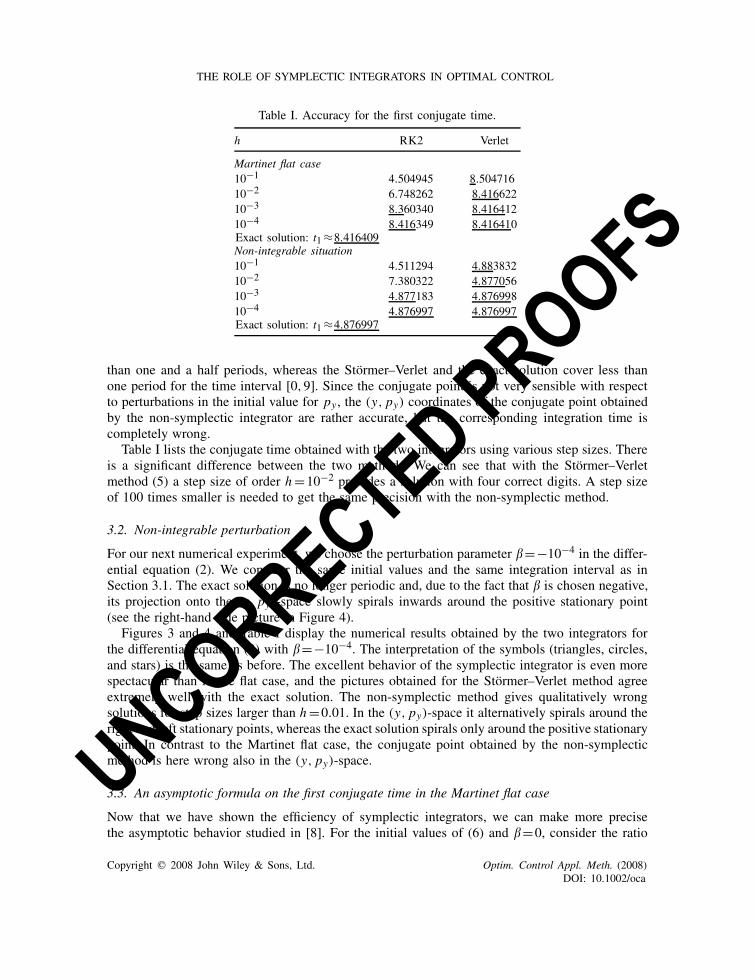
We consider first the flat case �=0 in the Hamiltonian system (2). As initial values we choose(cf. [8])

x(0)= y(0)= z(0)=0, px(0)=cos�0, py(0)= sin�0

pz(0)=10 where �0=�−10−3 (6)

so that we start close to an abnormal geodesics and integrate the system over the interval [0,9].Figure 1 displays the projection onto the (x, y)-plane of the numerical solution obtained with

different step sizes h by the two integrators. The initial value is at the origin, and the final state isindicated by a triangle. The circles represent the first conjugate point detected along the numericalsolution, whereas the stars give the position of the first conjugate point on the exact solution of theproblem. There is an enormous difference between the two numerical integrators. The symplectic


UNCORRECTED PROOFS


Figure 1. Trajectories in the (x, y)-plane for the flat case �=0.

Figure 2. Phase portraits in the (y, py)-plane for the flat case �=0.

(Stormer–Verlet) method (5) provides a qualitatively correct solution already with a large step sizeh=0.1, and it gives an excellent approximation for step sizes smaller than h=0.05. On the otherhand, the non-symplectic, explicit Runge–Kutta method (4) gives completely wrong results, andstep sizes smaller than 10−3 are needed to provide an acceptable solution. An explanation of thedifferent behavior of the two integrators is given in Section 4.

As noticed in Section 2, the normal geodesics in the flat case are determined by a one-degree-of-freedom Hamiltonian system in the variables y and py . We, therefore, show in Figure 2 theprojection onto the (y, py)-space of the solutions previously computed with step size h=0.05.The exact solution starts at (0,sin�0) above the saddle point, turns around the positive stationarypoint, crosses the py-axis at (0,− sin�0), turns around the negative stationary point and thencontinues periodically. The numerical approximation by the non-symplectic method covers more


UNCORRECTED PROOFS


Table I. Accuracy for the first conjugate time.

h RK2 Verlet

Martinet flat case10−1 4.504945 8.50471610−2 6.748262 8.41662210−3 8.360340 8.41641210−4 8.416349 8.416410Exact solution: t1≈8.416409Non-integrable situation10−1 4.511294 4.88383210−2 7.380322 4.87705610−3 4.877183 4.87699810−4 4.876997 4.876997Exact solution: t1≈4.876997

than one and a half periods, whereas the Stormer–Verlet and the exact solution cover less thanone period for the time interval [0,9]. Since the conjugate point is not very sensible with respectto perturbations in the initial value for py , the (y, py) coordinates of the conjugate point obtainedby the non-symplectic integrator are rather accurate, but the corresponding integration time iscompletely wrong.

Table I lists the conjugate time obtained with the two integrators using various step sizes. Thereis a significant difference between the two methods. We can see that with the Stormer–Verletmethod (5) a step size of order h=10−2 provides a solution with four correct digits. A step sizeof 100 times smaller is needed to get the same precision with the non-symplectic method.

3.2. Non-integrable perturbation

For our next numerical experiment, we choose the perturbation parameter �=−10−4 in the differ-ential equation (2). We consider the same initial values and the same integration interval as inSection 3.1. The exact solution is no longer periodic and, due to the fact that � is chosen negative,its projection onto the (y, py)-space slowly spirals inwards around the positive stationary point(see the right-hand side picture in Figure 4).

Figures 3 and 4 and Table I display the numerical results obtained by the two integrators forthe differential equation (2) with �=−10−4. The interpretation of the symbols (triangles, circles,and stars) is the same as before. The excellent behavior of the symplectic integrator is even morespectacular than in the flat case, and the pictures obtained for the Stormer–Verlet method agreeextremely well with the exact solution. The non-symplectic method gives qualitatively wrongsolutions for step sizes larger than h=0.01. In the (y, py)-space it alternatively spirals around theright and left stationary points, whereas the exact solution spirals only around the positive stationarypoint. In contrast to the Martinet flat case, the conjugate point obtained by the non-symplecticmethod is here wrong also in the (y, py)-space.

3.3. An asymptotic formula on the first conjugate time in the Martinet flat case

Now that we have shown the efficiency of symplectic integrators, we can make more precisethe asymptotic behavior studied in [8]. For the initial values of (6) and �=0, consider the ratio


UNCORRECTED PROOFS


Figure 3. Trajectories in the (x, y)-plane for the non-integrable case �=−10−4.

Figure 4. Phase portraits in the (y, py)-plane for the non-integrable case �=−10−4.

Figure 5. Illustration of the asymptotic behavior of R (Stormer–Verlet scheme with step size h=10−4).

R= t1√pz/(3K (k)), where t1 is the first conjugate time for the normal geodesic and K (k) is an

elliptic integral of the first kind

K (k)=∫ �/2

0

1√1−k2 sin2 u

du, k= sin(�0/2)


UNCORRECTED PROOFS


By studying the analytic solutions for the normal geodesics, it is proved in [8] that this ratiosatisfies the inequality 2

3�R�1. It follows from a rescaling of Equations (2) that R is independentof pz .

In Figure 5, we represent the values of 1−R as a function of �=�−�0, for various initialvalues �0. The numerical results indicate that the ratio R depends on �0, and R−→1− slowly for�0−→�−.

4. BACKWARD ERROR ANALYSIS

The theory of backward error analysis is fundamental for the study of geometric integrators andit is treated in much detail in the monographs of Sanz-Serna and Calvo [12], Hairer et al. [1,Chapter IX] and Leimkuhler and Reich [13]. It allows us to explain the numerical phenomenaencountered in the previous section.

4.1. Backward error analysis and energy conservation

We briefly present the main ideas of backward error analysis for the study of symplectic integrators,see [1, Chapter IX]. Consider a system of differential equations

y= f (y), y(0)= y0 (7)

and a numerical integrator yn+1=�h(yn) of order p. The idea is to search for amodified differentialequation written as a formal series in powers of the step size h,

˙y= f (y)= f (y)+h p f p+1(y)+h p+1 f p+2(y)+·· · (8)

such that yn = y(tn) for tn =nh, n=0,1,2, . . ., in the sense of formal power series. The motivationof this approach is that it is often easier to study the modified equation (8) than directly thenumerical solution.

What makes backward error analysis so important for the study of symplectic integrators is thefact that, when applied to a Hamiltonian system y= J−1∇H(y), the modified equation (8) has thesame structure ˙y= J−1∇ H (y) with a modified Hamiltonian

H(y)=H(y)+h pHp+1(y)+h p+1Hp+2(y)+·· ·However, the series usually diverges, so a truncation at a suitable order N(h) is necessary,

H (y)=H(y)+h pHp+1(y)+·· ·+hN−1HN (y)

This truncation induces an error that can be made exponentially small, by choosing N(h)∼C/h,see [1, Theorem IX.8.1]. More precisely, we have that for tn =nh and h→0,

H(yn)= H(y0)+O(tne−h0/h) (9)

as long as the numerical solution {yn} stays in a compact set. On intervals of length O(eh0/2h), themodified Hamiltonian H(y) is thus exactly conserved up to exponentially small terms.


UNCORRECTED PROOFS


4.2. Backward error analysis for the Martinet problem

Symplectic integrators are successfully applied in long-time integration of Hamiltonian systems,for instance in astronomy (e.g. the outer solar system over 100 million years [1, Section I.2.4]),or in molecular dynamics [13, Chapter 11]. The situation for the Martinet case is quite differentbecause we are interested in the numerical integration of Hamiltonian systems on relatively shorttime intervals. Nevertheless, symplectic integrators still reveal very efficient. Here, the essentialdifficulty is that the solution approaches a few times the critical point (y, py)=0 in the phasespace. We show in this section that symplectic integrators resolve close approaches to such acritical point with high accuracy even for large step sizes, whereas non-symplectic ones do notreproduce the correct behavior (except for very small step sizes).

4.2.1. Martinet flat case. Consider the Martinet problem (2) in the flat case �=0. Its interestingdynamics takes place in the (y, py) plane, and it is not influenced by the other variables (onlyby their initial values). We put �= (y, py), and we denote by f (�) the Hamiltonian vector fieldcomposed by the corresponding two equations of (2). For a numerical integrator of order p=2,the associated modified differential equation has the form

˙�= f ( �)+h2 f3( �)+O(h3) (10)

Consider first the symplectic Stormer–Verlet method. It follows from Section 4.1 that its modifieddifferential equation is Hamiltonian, and from (9) that the modified Hamiltonian H (�) is preservedup to exponentially small terms along the numerical solution. This implies that the numericalsolution remains exponentially close to a periodic orbit in the (y, py)-space. The critical point(y=0, py=0) is a saddle point also for the modified differential equation (because the originis stationary also for the numerical solution and thus for the modified equation). Therefore, anynumerical solution starting close to the origin has to come back to it after turning around one ofthe stationary points. The minimal distance to the origin will always stay the same (see the zoomin Figure 2). This explains the good behavior of symplectic integrators.

For the non-symplectic integrator, the term h2 f3(�) is not Hamiltonian. Therefore, the solutionof the modified differential equation (and hence also the numerical solution) is no longer periodic.In fact, it spirals outwards and after surrounding the first stationary point, the numerical solutiondoes not approach the saddle point sufficiently close, which induces a faster dynamics as canbe observed in Figures 1 and 2. This causes a huge error, because close to the saddle point thenumerical solution is most sensible to errors.

4.2.2. Non-integrable perturbation. In this case, the argument in the comparison of symplecticand non-symplectic integrators is very similar to the discussion of the Van der Pol’s equationin [1, Section XII.1]. For � �=0 (non-integrable perturbation), the dynamics takes place in thefour-dimensional space with variables �= (x, y, px, py). In this space, system (2) becomes

�= f (�)+�g(�)

where f (�) is the Hamiltonian vector field corresponding to �=0 and g(�)=O(1) dependssmoothly on �. Here, the modified equation becomes

˙�= f ( �)+�g( �)+h2 f3( �)+O(h3+�h2)

where the perturbation term h2 f3(�) is the same as for the Martinet flat case.


UNCORRECTED PROOFS


For the symplectic integrator, the perturbation �g(�) has the same effect for the original problemas for ˙�= f ( �)+h2 f3( �)+·· · . This explains the correct qualitative behavior for small h andsmall �. There is no restriction on the step size h compared with the size of �.

For the non-symplectic integrator, each of the perturbation terms �g(�) and h2 f3(�) destroysthe periodic orbits in the subsystem for the (y, py) variables, and the dominant one will determinethe behavior of the numerical solution. Only when h2|�|, the numerical solution will catch thecorrect dynamics of the problem. In Figures 3 and 4, where �=−10−4, this condition is not satisfiedfor h�10−2. Since � is chosen small and negative, the two perturbation terms are conflicting. Theterm �g(�) causes the solution to spiral around the positive stationary point, whereas the termh2 f3(�) causes it to spiral alternatively around both stationary points. For too large step sizes, thequalitative behavior of the non-symplectic integrator (4) is thus completely wrong.

RemarkProblem (2) with �=0 has a lot of symmetries. In the (y, py)-space the orbits are symmetric withrespect to the y-axis and also with respect to the py-axis. If we apply a symmetric numericalintegrator (not necessarily symplectic), it is possible to prove the same qualitative behavior as forthe symplectic Stormer–Verlet method. This follows from the fact that the solution of the modifiedequation (numerical orbit) corresponding to a symmetric method has the same symmetry propertiesas that of the exact flow (see [1, Section IX.2] for precise statements). Consequently, in the (y, py)plane and for �=0, the solution will stay exponentially near to a closed orbit, as it is the case forsymplectic integrators. In the non-integrable case, the good behavior of symmetric methods canbe explained as in Section 4.2.2 for symplectic methods.

5. ORBITAL TRANSFER OF A SPACECRAFT

We consider the orbit transfer problem presented in [14, pp. 66–68] and studied in [6]. Theproblem is to transfer a spacecraft with constant thrust force T from a given initial circular orbitr0 to the largest possible circular orbit for a given length of time t f . The control function is thethrust direction given by an angle (t). The state functions are (r,u,v), where r(t) is the radialdistance of spacecraft from attracting center, u(t) is the radial component of velocity and v(t) isthe tangential component of velocity.

The optimal control problem can be formulated as maximizing the radial distance r(t f ) at thefinal time, subject to the differential equations

r = u

u = v2

r−

r2+ T sin

m0−|m|tv = −uv

r+ T cos

m0−|m|t

(11)

with boundary conditions

r(0) = r0, u(t f )=0

u(0) = 0, v(t f )2r(t f )−=0

v(0) =√

r0

(12)


UNCORRECTED PROOFS


The constants are m0=10000kg (initial mass of spacecraft), |m|=12.9kg/day (fuel consump-tion rate), r0=1.496×1011m (distance Sun–Earth), T =8.336N (thrust force), =1.32733×1020m3/s2 (gravitational constant for sun) and t f =193 days (≈1.67×107 s).

We solve this problem using Pontryagin’s maximum principle. The Hamiltonian is

H = pru+ pu

(v2

r−

r2+ T sin

m0−|m|t)

+ pv

(−uv

r+ T cos

m0−|m|t)

+ pt (13)

and the differential equation for the adjoint state (pr , pu, pv, pt ) is

pr = pu

(v2

r2−2

r3

)− pv

uv

r2

pu = −pr + pvv

r

pv = −2puv

r+ pv

u

r

pt = −puT |m|

(m0−|m|t)2 sin− puT |m|

(m0−|m|t)2 cos, pt (0)=0

(14)

The extremality condition for p(t f ) is given by

pv(t f )v(t f )−2(pr (t f )−1)r(t f )=0 (15)

Applying the Pontryagin principle, the control (t) minimizes the Hamiltonian (13) at all times.This yields

sin()= −pu√p2u+ p2v

, cos()= −pv√p2u+ p2v

The Hamiltonian system (11) and (14) with boundary conditions (12) and (15) is solved by thestandard single shooting technique. In Figure 6, we plot the exact solution (computed numericallywith high precision). The thrust direction starts close to the tangential direction and rotatesduring the orbit transfer with an angle of about ≈2�. At the middle of the time interval, the thrustdirection rotates more rapidly.

In Figure 7 we plot the relative errors in the Hamiltonian as functions of time (comparedwith the Hamiltonian of the exact solution) for various symplectic and non-symplectic numericalintegrators of orders 1, 2 and 3. We do not observe any significant advantage for the symplecticintegrators. We notice a qualitative different behavior of the methods of order 2. There, the error inthe Hamiltonian has a peak in the middle of the integration interval, and it comes back to about thesame value it had before. For the midpoint rule this is due to its symmetry, and for the second-orderRunge–Kutta methods this follows from the fact that for methods with even order the dominanterror term behaves like that of a symmetric integrator (backward error analysis). The results ofthis experiment are not really surprising, because the solution does not have a quasi-oscillatorybehavior, so that errors in the Hamiltonian could be compensated by a symplectic integrator.


UNCORRECTED PROOFS


Figure 6. Exact solution of the orbit transfer problem on the time interval [0, t f ].

Figure 7. Errors in the Hamiltonian for various numerical integrators applied with constant step size (1000steps). Explicit Runge–Kutta methods (non-symplectic) of orders 1, 2, 3 (RK1, RK2, RK3) compared

with the symplectic Euler method (order 1) and the implicit midpoint rule (order 2, symplectic).

6. SUBMERGED RIGID BODY

We consider the autonomous submarine model introduced in [15]. For simplicity, we restrictourself to the vertical planar situation: the rigid body moves in the xz-plane exclusively. Thestate of the rigid body is given by q(t)= (b1(t),b3(t),�(t),�1(t),�3(t),�2(t)), where b1(t),b3(t)denote the position vector and �(t) represents the diving angle, and �1(t),�3(t), and �2(t) are thecorresponding translational and angular velocities.

Given a fixed time interval of length t f >0, we search for the energy minimizing trajectory toget the submarine from a configuration q(0) to a configuration q(t f ), e.g. t f =5 and

q(0)= (0,0,0,0,0,0), q(5)= (1,1,0,0,0,0)

Here, the energy is defined as (a more realistic energy model is derived in [16])

E(q)= 1

2

∫ t f

0(�2

�1 +�2�3 + 2�2

)dt


UNCORRECTED PROOFS


where ��1(t),��3(t) and �2(t) are the control functions. The dynamics are

b1 = �1 cos�+�3 sin�, �1= 1

m1(−m3�3�2−D2

� �31−D1

� �1+G sin�+��1)

b3 = −�1 sin�+�3 cos�, �3= 1

m3(m1�1�2−D2

� �33−D1

� �3−G cos�+��3)

� = �2, �2= 1

Ib2(−D2

��32−D1

��2+�gV(−zB sin�+xB cos�)+ �2)

with positive constants m1=m3=m+M (masses), m=126.55kg, M=70kg, D1� =−27.0273,

D2� =−897.6553,D1

�=−13.793,D2�=−6.45936 (drags), G=−3N (Archimede), Ib2=5.29kgm2,

g=9.80ms−2, �gV=mg−G, zB =−7×10−3m, xB =0m (buoyancy). These numerical valueswere derived from experiments performed on a test-bed vehicle, see [15].

Here, the Hamiltonian system is very sensitive when considered as an initial value problem (i.e.q(0) and p(0) given). When one slightly perturbates initial conditions (e.g. by multiplying p(0) orq(0) by 1+10−10), the corresponding solution explodes. For this reason, single shooting methodsfail to solve the boundary value problem, and we use a multiple shooting method.

For this system we found one normal extremal with a conjugate point. The corresponding states,costates and controls are represented in Figure 8 (using a high-order integrator).

In Figure 9, we compare for the same step size (h=0.05) the accuracy of the implicit midpointrule (order 2), which is a symplectic integrator, with an explicit Runge–Kutta method (non-symplectic) of the same order (RK2, see (4)). The numerical solution and the determinant of theJacobian �q/�p0 are obtained on the grid points of integration. For the computation of conjugatepoints we need a continuous approximation of the solution, which is obtained by cubic Hermiteinterpolation. The resulting interpolation error is of size O(h4) and thus negligible for second-ordermethods. Notice that linear interpolation would introduce an error O(h2) that is of the same sizeas the truncation (global) error of the numerical integrators. The mark in the middle of Figure 9corresponds to the conjugate point of the exact solution. There is again no real advantage for thesymplectic integrator. The implicit midpoint rule (symplectic) is only twice more accurate thanthe non-symplectic method RK2, and this is due to the size of the error constants of the methodsand not to symplecticity.

Figure 8. Extremal obtained for p(0)=(7709.864500233298,7988.036994413952,−3.0163588901640024,11707.858394005056,12318.149504556683,−1.0570538454444238).


UNCORRECTED PROOFS


Figure 9. Computation of det�q/�p0. Left picture: exact solution on the time interval [0,5]. Right picture:implicit midpoint rule (symplectic) and an explicit Runge–Kutta method (RK2, non-symplectic) for the

same step size h=0.05 with cubic Hermite interpolation.

7. CONCLUSIONS

From the ‘geometric numerical integration’ point of view, it is natural to use symplectic integratorswhen solving Hamiltonian differential equations. This has been proved very successfully in manyfields, in particular, in molecular dynamics simulations and in long-time integrations of planetarymotion. For Hamiltonian systems arising from the Pontryagin maximum principle in optimalcontrol, our conclusion is the following.

Owing to the fact that one is concerned with boundary value problems, long-term integrationis not an issue. For integrations over short intervals, e.g. half a period on the motion of a planet,there is no real advantage of using a symplectic method. The solutions of problems of Sections 5and 6 neither show a periodic or quasi-periodic behavior nor a ergodic behavior like in moleculardynamics simulations. Therefore, no improvement in symplectic integrators can be expected, whichis confirmed by numerical experiments.

For special problems, typically in low dimension and in situations where the Hamiltonian is closeto a critical value (Section 3), the structure preservation of symplectic integrators is very importantand symplectic methods can be much more efficient than the non-symplectic ones. Indeed, thetheory of backward error analysis allows one to prove that the numerical solution of a symplecticmethod has the same qualitative behavior as the exact flow. For example, in the integrable Martinetcase, where the exact solution is periodic, the numerical solution remains exponentially close to aperiodic orbit, which explains the excellent results, even on a relatively short interval of integration(a few periods). For non-symplectic integrators, this structure is destroyed in general.

ACKNOWLEDGEMENTS

This work was partially supported by the Fonds National Suisse, project No. 200020-109158 and by theNational Science Foundation grant DMS-030641.

REFERENCES

1. Hairer E, Lubich C, Wanner G. Geometric Numerical Integration. Structure-preserving Algorithms for OrdinaryDifferential Equations (2nd edn). Springer Series in Computational Mathematics, vol. 31. Springer: Berlin, 2006.

2. Wendlandt JM, Marsden JE. Mechanical integrators derived from a discrete variational principle. Physica D1997; 106:223–246.


UNCORRECTED PROOFS


3. Marsden JE, West M. Discrete mechanics and variational integrators. Acta Numerica 2001; 10:357–514.4. Bloch AM, Crouch PE, Marsden JE, Ratiu TS. The symmetric representation of the rigid body equations and

their discretization. Nonlinearity 2002; 15:1309–1341.5. Guibout V, Bloch A. A discrete maximum principle for solving optimal control problems. 43rd IEEE Conference

on Decision and Control, Atlantis, Paradise Island, Bahamas, vol. 2, December 2004; 1806–1811.6. Hager W. Runge–Kutta methods in optimal control and the transformed adjoint system. Numerische Mathematik

2000; 87(2):247–282.7. Bonnans JF, Laurent-Varin J. Computation of order conditions for symplectic partitioned Runge–Kutta schemes

with application to optimal control. Numerische Mathematik 2006; 103(1):1–10.8. Agrachev AA, Bonnard B, Chyba M, Kupka I. Sub-Riemannian sphere in Martinet flat case. ESAIM—Control

Optimisation and Calculus of Variations 1997; 2:377–448.9. Bonnard B, Chyba M, Kupka I. Non integrable geodesics in SR-Martinet geometry. Proceedings of the Symposium

on Pure Mathematics, vol. 64. American Mathematical Society: Providence, RI, 1999; 119–134.10. Bonnard B, Launay G, Trelat E. The transcendence needed to compute the sphere and wave front in Martinet

SR-geometry. Journal of Mathematical Sciences 2001; 103(6):688–708.11. Bonnard B, Trelat E. On the role of abnormal minimizers in SR-geometry. Annales de la Faculte des Sciences

de Toulouse Mathematiques 2001; 6(X, 3):405–491.12. Sanz-Serna JM, Calvo MP. Numerical Hamiltonian Problems. Chapman & Hall: London, 1994.13. Leimkuhler B, Reich S. Simulating Hamiltonian Dynamics. Cambridge Monographs on Applied and Computational

Mathematics, vol. 14. Cambridge University Press: Cambridge, 2004.14. Bryson Jr AE, Ho Y-C. Applied Optimal Control. Blaisdell: Waltham, MA, 1969.15. Chyba M, Haberkorn T, Smith RN, Choi SK. Design and implementation of time efficient trajectories for

underwater vehicles. Journal of Ocean Engineering 2008. DOI: 10.1016/j.oceaneng.2007.07.007.16. Chyba M, Haberkorn T, Smith RN, Choi SK. Autonomous underwater vehicles: development and implementation

of time and energy efficient trajectories. Ship Technology Research 2008; 55(2):36–48.


UNCORRECTED PROOFS

Date post:	11-Feb-2022
Category:	Documents
Upload:	others
View:	2 times
Download:	0 times

UNCORRECTED PROOFS - Department of Mathematics - University

Documents