Understanding the Factors Behind Crude Oil Price Changes · The purpose of this thesis is to...

Master's thesis

Trondheim, June 2010

Norwegian University of Science and TechnologySocial Science and Technology ManagementIndustrial Economics and Technology Management

Academic supervisor: Stein-Erik Fleten

Mats OlimbTore Malo Ødegård

Understanding the FactorsBehind Crude Oil PriceChangesA Time-varying Model Approach

NTNUNorwegian University ofScience and Technology

Field of study

Start date

Title

MASTER THESIS

for

STUD.TECHN TORE MALO ODEGARD AND MATS OLIMB

Financial EngineeringInvestering, finans og okonomistyring

1s.01.2010

Understanding the factors behind crude oil price changesUnderliggende faktorer bak bevegelser i oljeprisen

Oil price movements have been a subject of discussion for centuries. In recentyears, economists and policy makers have shown increasing concems

regarding speculation and extreme oil price movements. In this thesis weindentifu and evaluate main factors behind oil price changes.

Faculty of Social Sciencesand Technology Management

Department of Industrial Economicsand Technolory Management

Stein-Erik FletenSupervisor

Purpose

Main contents:

Description of main factors behind oil price movementsDevelop an empirical model for oil price changes to study developments over time and theirsignificance.

1.

2.

M(*,^Qk S,k*e^afU-k,^Monica Rolfsen

Deputy Head of Department

DECLARATION

Stud.techn. MATS OLIMB

Department of Industrial Economics and Technology Management

I hereby declare that I have written the above mentioned

thesis without any kind of illegal assistance.

TRONDHEIM Place Date

Signature

In accordance with Examination regulations § 20, this thesis, together with its figures etc., remains the property of the Norwegian University of Science and Technology (NTNU). Its contents, or results of them, may not be used for other purposes without the consent of the interested parties.

DECLARATION

Stud.techn. TORE MALO ØDEGÅRD

Department of Industrial Economics and Technology Management

I hereby declare that I have written the above mentioned

thesis without any kind of illegal assistance.

TRONDHEIM Place Date

Signature

In accordance with Examination regulations § 20, this thesis, together with its figures etc., remains the property of the Norwegian University of Science and Technology (NTNU). Its contents, or results of them, may not be used for other purposes without the consent of the interested parties.

Preface

This master thesis was written at the Norwegian University of Science and Technology (NTNU),

department of Industrial Economics and Technology Management, during the spring of 2010. The thesis

is written within the field of Financial Engineering. The idea behind the thesis stems from the Project

thesis written in the autumn of 2009 (Olimb & Ødegård, 2010), and ideas and thoughts of Jussi Keppo at

the University of Michigan.

We would like to thank our supervisor, professor Stein-Erik Fleten (NTNU) for constructive feedback and

contributing with guidelines on academic writing. We are also grateful to Johan Magne Sollie (NTNU)

for guidance on the econometric framework and methods. Finally, we would like to express our gratitude

to Torbjørn Kjus (DnB NOR Markets) for providing us with useful data and insights on the crude oil

market.

Trondheim, June 4th 2010.

____________________ ______________________

Mats Olimb Tore Malo Ødegård

Abstract

This thesis investigates the underlying factors behind the crude oil price changes, using a time-varying

approach for the period from 1995 to 2009. The analysis is an extension of previous studies of oil market

determinants, and is to our knowledge the only time-varying analysis for a broader set of explanatory

variables. By allowing the parameter coefficients to vary over time, we are able to identify and describe

structural changes in the crude oil market during the time period studied. Our analysis suggests that the

crude oil market participants have been more focused on expectations, and draw less attention to

fundamental factors, during the time period examined. We do not find that the positions of financial

investors by itself cause changes in the crude oil price significantly. However, we show that the entry of

new market participants have influenced changes in the process of crude oil price setting, which has

become more similar to the process in financial markets. The time-varying analysis also reveals that

changes in world economic activity have a particularly strong relationship with crude oil price changes

during economic recessions. We find that OPEC has been an important factor in recent years, not in virtue

of being a price setter, but by the organization’s diminishing ability to operate as swing producer. Lack of

OPEC spare capacity in the recent years caused large imbalances in the world crude oil market, as OPEC

historically has represented the only major buffer on the supply side.

Table of contents 1.Introduction ................................................................................................................................................ 1

1.1 Crude oil market characteristics .......................................................................................................... 1

1.2 Related studies on the crude oil market .............................................................................................. 2

1.3 Focus and factors ................................................................................................................................ 3

2.The Crude oil market ................................................................................................................................. 5

2.1 Demand ............................................................................................................................................... 5

2.2 Supply ................................................................................................................................................. 5

2.3 Volatility ............................................................................................................................................. 7

2.4 Futures market and speculators ........................................................................................................... 7

2.5 Market factors ..................................................................................................................................... 8

2.6 Summary of hypotheses .................................................................................................................... 14

3.Data .......................................................................................................................................................... 15

3.1 Data description ................................................................................................................................ 15

3.2 Descriptive statistics ......................................................................................................................... 20

4.Methodology ............................................................................................................................................ 24

5.Empirical results ...................................................................................................................................... 28

5.1 Model selection ................................................................................................................................. 28

5.2 Time-varying coefficients ................................................................................................................. 31

5.3 Granger-causality .............................................................................................................................. 36

5.4 OPEC’s influence on crude oil prices ............................................................................................... 39

5.5 Future expectations affecting crude oil prices .................................................................................. 42

5.6 Model weaknesses and alternative approaches ................................................................................. 43

6.Conclusions .............................................................................................................................................. 45

References ................................................................................................................................................... 46

Appendix ..................................................................................................................................................... 49

A.1 Individual time-varying coefficient plots ......................................................................................... 49

A.2 Correlation-matrices ......................................................................................................................... 50

A.3 Rolling correlation plots ................................................................................................................... 51

A.4 Statistical concepts used ................................................................................................................... 52

A.5 Cost-of-carry model ......................................................................................................................... 58

A.6 Time-varying coefficient plots including MSCI factor .................................................................... 59

List of figures Figure 1: Exploration and production spending ............................................................................................ 6

Figure 2: Open interest .................................................................................................................................. 8

Figure 3: Changes in NYMEX futures contracts ........................................................................................ 12

Figure 4: Time series plot ........................................................................................................................... 19

Figure 5: Plot of transformed data .............................................................................................................. 22

Figure 6: Chow test graphics ...................................................................................................................... 30

Figure 7: Time-varying beta coefficients .................................................................................................... 31

Figure 8: Residual graphics for the state space model ................................................................................ 32

Figure 9: Time varying beta coefficients for the OPEC model .................................................................. 40

Figure 10: Residual graphics for the OPEC model ..................................................................................... 40

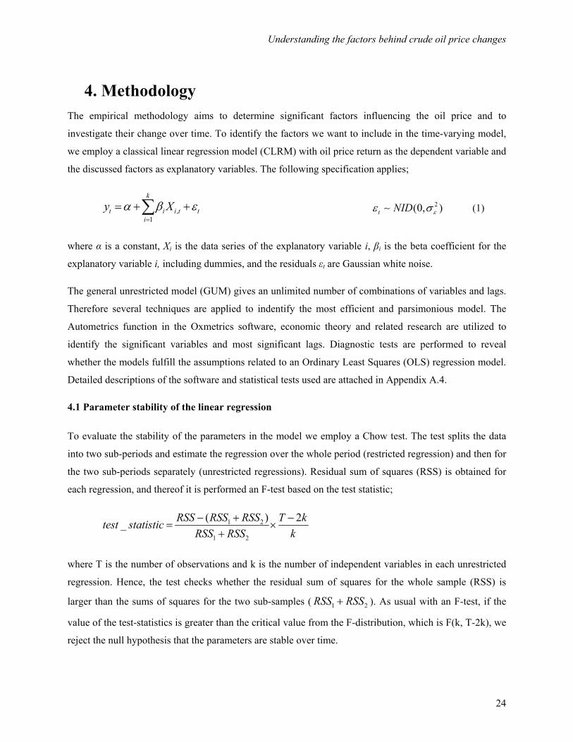
Figure 11: Time-varying coefficient for the MSCI factor .......................................................................... 43

Figure 12: Time-varying beta coefficients for the state-space model, analyzed individually .................... 49

Figure 13: Rolling correlations ................................................................................................................... 51

Figure 14: Time-varying coefficients including the MSCI factor .............................................................. 59

List of tables Table 1: Summary of hypotheses ................................................................................................................ 14

Table 2: Dummy variables .......................................................................................................................... 18

Table 3: Descriptive statisitcs ..................................................................................................................... 23

Table 4: Linear regression model................................................................................................................ 28

Table 5: Summary of test statistics for the state-space model .................................................................... 31

Table 6: Granger-causality test ................................................................................................................... 38

Table 7: Summary of test statistics for the OPEC model ............................................................................ 41

Table 8: Correlation matrix, time series ...................................................................................................... 50

Table 9: Correlation matrix, transformed data ............................................................................................ 50

Understanding the factors behind crude oil price changes

1

1. Introduction

The purpose of this thesis is to analyze factors affecting change in the crude oil price over the period from

1995 to 2009. We apply a time-varying model to analyze how significant factors vary over time; that is,

how the different underlying explanatory factors’ relationship with crude oil prices behave stochastically.

Crude oil prices have been the source of discussion over the past decades. The cyclical nature of the

market in times of under- and overinvestment has made it challenging for countries, industrial companies

and investors to deal with the risks involved. It is believed that high oil prices can slow economic growth,

cause inflationary pressures and create global imbalances. Volatile prices can also increase insecurity and

discourage essential investments in the oil sector. Recent high oil prices and tight market conditions have

also raised fears about oil scarcity and concerns about energy security in many oil-importing countries.

An in-depth analysis of the underlying factors can be useful to anyone dependent on or interested in

investing in the crude oil market. The empirical evidence may help to improve understanding of the

behavior of the underlying factors and the market dynamics. Analysis of time-varying coefficients will

not only identify which factors are significant over the time period studied, but also which factors that

have relatively fixed behavior and those that behave differently through different periods of an economic

cycle.

1.1 Crude oil market characteristics

Crude oil prices should priced much like any other exhaustible commodity (Hotelling, 1931), yet there is

a common belief that oil and energy prices behave differently and are more volatile than other

commodities (Fleming & Ostdiek, 1999). Some observers also argue that the crude oil market has

undergone structural transformations that have changed the influence of underlying factors and placed the

oil price on a new path. One special point concerning price formation in the crude oil market is the

Organization of the Petroleum Exporting Countries (OPEC), which operates as a cartel with the largest

production capacity. Crude oil price cycles are common and may extend over several years responding to

changes in demand as well as OPEC and non-OPEC supply. The underlying factors’ influence on price

movements will vary during the cycle depending on the position in the cycle, pace and future

expectations. As an example, the pricing power of OPEC is not straightforward. The pricing power varies

over time and is induced by market conditions and can be seen in both weak and tight markets (Fattouh,

2007a).


2

A point made by Fattouh (2007a) is with the growing importance of the futures market in the process of

price discovery; it has become more difficult for producers and especially OPEC to follow set output

policies. This point might be especially important as the last years have seen a strong growth in the

commodity derivatives markets. The total value of the investment in commodity indexes has increased

from about 15 billion in 2003 to above 200 billion US Dollars by mid-2008 (US Senate, 2009). During

this period, financial institutions have heavily marketed commodity indexes as a way to diversify

portfolios, and profit from rising commodity prices. About 70 percent of the commodity index

investments are invested in near-term energy contracts, following a strategy of continuously rolling

futures contracts to maintain the investment (Hamilton, 2008).

1.2 Related studies on the crude oil market

Three main approaches have been used for analyzing oil prices. First, non-structural models rely on the

theory of exhaustible resources as the basis for understanding the oil market. Second a structural

supply/demand framework uses behavioral equations and factors that link oil demand and supply to its

various determinants. Finally, an informal approach can be studied by analyzing oil price movements

within specific contexts and episodes of oil market history (Fattouh, 2007a). In this thesis we will utilize a

structural framework when analyzing underlying factors behind oil price changes, and we will also seek

to identify structural changes through a time-varying framework. We go through the literature of

structural studies on price determinants in an econometric framework.

Kaufmann et al. have performed several econometric analyses of oil prices. In their first paper (Kaufmann

R. , Dèes, Karadeloglou, & Sanchez, 2004) a linear regression model is studied to investigate OPEC’s

ability to influence real oil prices. Three coefficients; OPEC capacity utilization, quotas and the degree to

which production exceeds these quotas are studied along with OECD stocks of crude oil, and are all found

to be significant. They also show that the direction of causality generally runs from the explanatory

variables to real oil prices. We will utilize the same three OPEC variables as supply variables to analyze

OPEC’s influence on oil prices, and also investigate the direction of causality.

Kaufmann et al. (2008) expands their previous models for crude oil prices to include refinery utilization

rates, OPEC capacity utilization and contango level as explanatory variables to explain the rapid rise in

crude price between 2004 and 2006. They conclude that most of the increase can be explained by

concerns about future oil market conditions, represented by the future market moving from backwardation

to contango. In our time-varying model we will investigate the significance of three future market

variables to study this further.


3

Möbert (2007) replicates the OPEC model defined by Kaufmann et al. (2004) and finds that the

parameters are not stable after the market turmoil seen after September 11 2001. The analysis is extended

with the previous data continued to 2006. He specifies an econometric model based on a larger set of

covariates, including supply and demand variables as well as futures market variables. The findings show

that these variables might be better when explaining recent price movements. Current price movements

are shown to be a result of scarce refinery capacity and speculators betting on higher prices. Möbert’s

findings support our suspicion that underlying factors are not stable during longer economic cycles. It also

supports our choice of investigating a larger econometric model.

Tham (2008) is to our knowledge the only paper studying time-varying factors behind the oil price. A set

of four explanatory variables are used to explain price movements, including contango/backwardation

level, refinery utilization, days of stock cover and non-commercial long ratio, for the time period from

1995:5 to 2008:2. Results indicate an increasing sensitivity of the oil price to speculation since 2004. All

explanatory variables show increasing explanatory power. The time period analyzed only includes one

business cycle and ends close to the level where crude oil prices peaked in July 2008. Including the recent

market downturn and a larger set of covariates should give us a better understanding of the dynamics in

the crude oil market.

Hamilton (2008) examines factors responsible for recent changes in crude oil prices, and especially what

produced the high price in the summer of 2008. The factors are not implemented in a model but discussed

to get a broader understanding. Factors include commodity price speculation, strong world demand, time

delays or geological limitations on increasing production, OPEC monopoly pricing, and an increasingly

important contribution of the scarcity rent1. One conclusion is that rather to think of the individual factors

as competing hypotheses when explaining recent price movements, such as the soaring prices in 2008;

one possibility is that there is an element of explanation to a broader set.

1.3 Focus and factors

We identify and study the significant underlying factors in a state-space framework. The thesis examines

the dynamics, structural breaks and the fluctuations of the underlying factors in the crude oil market. We

extend the research of Möbert, Tham and Hamilton by examining demand, supply, OPEC’s influence,

financial factors and price speculation simultaneously for their impact on crude oil price changes in a

state-space model during the time period from 1995 to 2009. 1 The marginal opportunity cost imposed on future generations by extracting one more unit of a resource today. Scarcity rent is

the cost of depleting a finite resource because benefits of the extracted resource are unavailable to future generations.


4

Two contributions are made to the literature. First, we expand the time-varying model set out by Tham

(2008) to include a broader set of explanatory factors and the recent financial crisis. Second, we show that

no single market factor can exclusively explain crude oil price changes in any of the months studied. Our

results indicate that rather looking towards one cause of longer-term oil price movements there might be

an explanatory effect to a broader set simultaneously.

Our model identifies eight significant factors when explaining crude oil price changes for the time period.

One factor for demand; changes in world economic growth, three factors for the supply side; changes in

rig utilization, days of stock cover and refinery utilization and two factors for the financial markets;

changes in contango level and non-commercial open interest long ratio, are found to be significant.

Finally we also found significant effects on two OPEC factors; changes in OPEC spare production

capacity and production quotas.

The time-varying parameters show that crude oil price changes have become more sensitive to world

economic activity during time periods of economic recessions and by future expectations to crude oil

demand after 2005. Supply fundamentals in the upstream sector and spare production capacity

represented by OPEC have increased their influence in the tight market conditions seen before the

financial crisis. However, the other supply fundamentals have low explanatory power, especially in the

time period after 2005. The futures market position has also become less important through the time

period, indicating a loosening in the relationship between weak and tight supply fundamentals and the

changes in crude oil price. This is also shown by the diminishing relationship between crude oil price

changes and refinery utilization rates.


5

2. The Crude oil market

2.1 Demand

Oil prices are linked, like those of other commodities, to the level of economic activity in the

industrialized countries. Demand, both from consumers and the industrial sector, increases with economic

and population growth, and slow down when economic growth rates decline. The demand for oil is also

affected by factors such as the exchange rate, depending on the country being a net importer or exporter

of crude oil, and the rate of industrialization in developing countries.

Oil importing countries, such as the US, will increase their oil demand as a result of economic growth. In

oil exporting countries it is likely that an expansion in the oil sector has led to growth in GDP, as has been

the case for countries like Russia and Saudi Arabia. In these countries, high oil prices based on rising oil

demand create an inflow of oil derived revenue, increasing economic growth. If oil prices stabilize at too

high levels, economic growth in importing nations might decline, causing a decline in demand and prices

of oil (Priog, 2005). High prices will also lead to increases in exploration and development budgets

leading to new oil discoveries and increased supply which over time will cause prices to decline. High

prices can also make alternative fuels more competitive; potentially reducing the demand for oil.

The United States has historically been the single biggest consumer of crude oil, consuming 22.5 percent

of the world output in 2008 (BP, 2009), but consumption has shown a flat or downward development

since 2005. Recent growth in world oil consumption has come from non-OECD countries, and especially

China and Saudi Arabia (BP, 2009), which also display the highest economic growth.

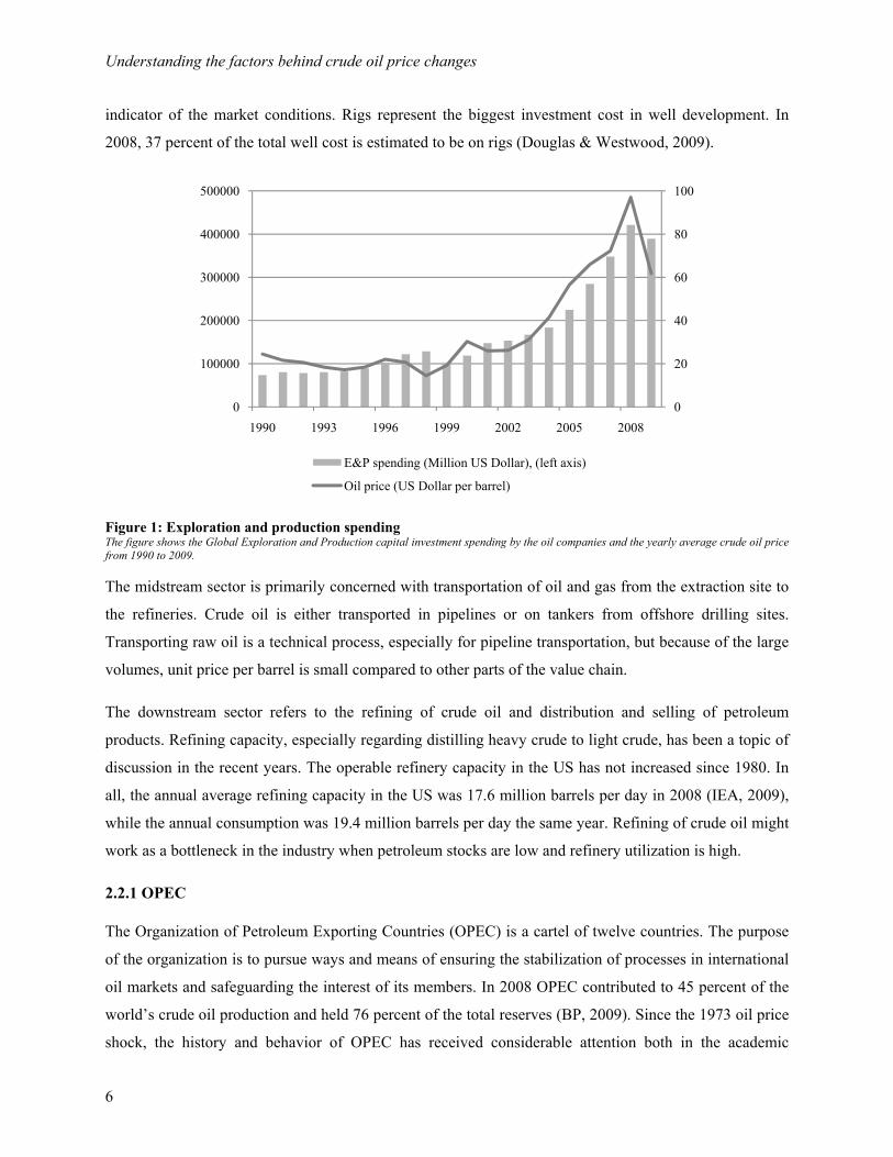
2.2 Supply

The petroleum industry is divided into three sectors; the upstream, midstream and downstream sector. The

upstream sector consists of the exploration and production (E&P) business. An important indicator of the

activity level within the E&P sector is the oil companies’ capital investment budgets. Many economists

have blamed underinvestment in the sector on the tight market and price increases in the period from

2005 to 2008 (Fattouh & Mabro, 2006). The budget numbers are however complicated to use in an

econometric analysis since budgets are built on other factors like complexity level (of a field

development) and cost inflation within the sector, in addition to the current activity level. The E&P sector

is considered to be the bottleneck in the industry, and the most important since it determines the supply of

crude oil which affects prices in the downstream sector. Bottlenecks become evident in tight market

conditions, which is hard to measure directly in the upstream sector. We will use rig utilization rates as an


6

indicator of the market conditions. Rigs represent the biggest investment cost in well development. In

2008, 37 percent of the total well cost is estimated to be on rigs (Douglas & Westwood, 2009).

Figure 1: Exploration and production spending The figure shows the Global Exploration and Production capital investment spending by the oil companies and the yearly average crude oil price from 1990 to 2009.

The midstream sector is primarily concerned with transportation of oil and gas from the extraction site to

the refineries. Crude oil is either transported in pipelines or on tankers from offshore drilling sites.

Transporting raw oil is a technical process, especially for pipeline transportation, but because of the large

volumes, unit price per barrel is small compared to other parts of the value chain.

The downstream sector refers to the refining of crude oil and distribution and selling of petroleum

products. Refining capacity, especially regarding distilling heavy crude to light crude, has been a topic of

discussion in the recent years. The operable refinery capacity in the US has not increased since 1980. In

all, the annual average refining capacity in the US was 17.6 million barrels per day in 2008 (IEA, 2009),

while the annual consumption was 19.4 million barrels per day the same year. Refining of crude oil might

work as a bottleneck in the industry when petroleum stocks are low and refinery utilization is high.

2.2.1 OPEC

The Organization of Petroleum Exporting Countries (OPEC) is a cartel of twelve countries. The purpose

of the organization is to pursue ways and means of ensuring the stabilization of processes in international

oil markets and safeguarding the interest of its members. In 2008 OPEC contributed to 45 percent of the

world’s crude oil production and held 76 percent of the total reserves (BP, 2009). Since the 1973 oil price

shock, the history and behavior of OPEC has received considerable attention both in the academic

0

20

40

60

80

100

0

100000

200000

300000

400000

500000

1990 1993 1996 1999 2002 2005 2008

E&P spending (Million US Dollar), (left axis)

Oil price (US Dollar per barrel)


7

literature and in the media. Conflicting academic and empirical interpretations about the influence of

OPEC on the world oil markets have been proposed. OPEC is a swing producer and “sets production

quotas based on its assessment of the market’s call on its supply. Oil prices fluctuate in part according to

how well OPEC performs this calculation. Through the process of adjusting its production quotas, OPEC

can only hope to influence price movements towards a target level or target zone. In a supply-demand

framework, the oil price is determined by OPEC and non-OPEC supplies as well as oil arriving to the

market from OPEC members who do not abide by the assigned quotas” (Fattouh, 2007b).

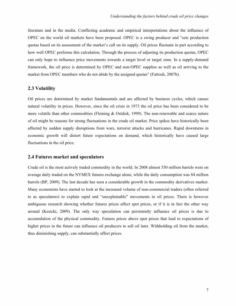
2.3 Volatility

Oil prices are determined by market fundamentals and are affected by business cycles, which causes

natural volatility in prices. However, since the oil crisis in 1973 the oil price has been considered to be

more volatile than other commodities (Fleming & Ostdiek, 1999). The non-renewable and scarce nature

of oil might be reasons for strong fluctuations in the crude oil market. Price spikes have historically been

affected by sudden supply disruptions from wars, terrorist attacks and hurricanes. Rapid downturns in

economic growth will distort future expectations on demand, which historically have caused large

fluctuations in the oil price.

2.4 Futures market and speculators

Crude oil is the most actively traded commodity in the world. In 2008 almost 550 million barrels were on

average daily traded on the NYMEX futures exchange alone, while the daily consumption was 84 million

barrels (BP, 2009). The last decade has seen a considerable growth in the commodity derivatives market.

Many economists have started to look at the increased volume of non-commercial traders (often referred

to as speculators) to explain rapid and “unexplainable” movements in oil prices. There is however

ambiguous research showing whether futures prices affect spot prices, or if it is in fact the other way

around (Kesicki, 2009). The only way speculation can persistently influence oil prices is due to

accumulation of the physical commodity. Futures prices above spot prices that lead to expectations of

higher prices in the future can influence oil producers to sell oil later. Withholding oil from the market,

thus diminishing supply, can substantially affect prices.


8

Figure 2: Open interest The figure shows the number of outstanding contracts (open interest) for all crude oil contracts traded on NYMEX. The commercial open interest is displayed on the left axis and the non-commercial open interest on the right axis. Each contract is for 1000 barrels of oil.

2.5 Market factors

2.5.1 Demand

Unlike Möbert (2007) we will not use direct data for demand to avoid problems with simultaneity. We

use the two same proxies for demand as Kaufmann (2005); gross domestic product and exchange rates. In

contrast to Kaufmann (2005) we do not estimate demand equations for ten main economies, but use world

economic growth and exchange rate index for the US Dollar to obtain a proxy for the global crude oil

demand.

World economic growth

The scale and the activity level of the economy is an essential factor that affects crude oil demand.

Industrialized countries have a higher demand for crude oil, while developing countries represent the

biggest growth in crude oil demand. We expect economic growth to have a significant positive

relationship with crude oil price changes.

Exchange rate

US Dollar is the currency of choice in global crude oil trade while consumers use local currencies to buy

petroleum products. When the US Dollar depreciates against other currencies, countries with non-dollar

appreciating currencies enjoy cheap oil, while consumers in US Dollar-pegged countries pay a higher

price for the same barrel of oil. Changes in the US Dollar will therefore affect world oil demand.

Depreciation (appreciation) of the US Dollar versus other currencies will decrease (increase) the cost of

0

50000

100000

150000

200000

250000

300000

100000

250000

400000

550000

700000

850000

1000000

1995 1997 1999 2001 2003 2005 2007 2009

Commercial (left axis)

Non-commercial


9

buying a dollar and hence also a barrel of oil. This will increase (decrease) the demand for crude oil, in

other currencies than the US Dollar, and also the price. We therefore expect a negative relationship

between the US Dollar exchange rate and the crude oil price changes.

2.5.2 Supply

The supply variables investigated are similar to Kaufmann et al. (2008), Möbert (2007) and Tham (2008),

with the exception of tanker charter rates, which is included to investigate the effect any possible

bottlenecks in the midstream sector might have on the crude oil price.

Rig utilization

To investigate the relationship between activity levels in the upstream sector, the number of active rigs

utilized is used as a proxy. There is an extensive time lag (5-10 years) between exploration drilling and

production, but the utilization of rigs is a good indicator of the activity level in the upstream sector and on

the future expected oil supply. The relationship between the number of active rigs and the crude oil price

is ambiguous. High drilling activity is a sign of increased production and supply, and should in the long-

term have a negative relationship with crude oil prices. On the other side, drilling activity is also

dependent on the ease of financing for oil companies and the economic activity. Drilling is capital

intensive and will depend on the companies’ current and expected future cash flows, which again is

affected by the oil prices and economic activity. New rigs also require a lot of resources which again will

have a positive impact on oil prices. We expect a positive relationship between rig utilization and crude

oil price changes.

Crude tanker charter rates

Tanker charter rates are dependent on demand and fleet size in the tanker shipping market. The

relationship between charter rates and crude oil prices is expected to be positive, but not significant since

transportation costs are only a small part of total per barrel cost. Therefore, we do not expect that these

factors influence the oil supply noticeably. It is more reasonable to believe that the supply bottleneck is in

the upstream- or downstream sector. However, we choose to include this variable in the analysis before

reaching any conclusion, and charter rates are depicted as the best indicator on the midstream sector.

Refinery Utilization

Refinery utilization rates affect crude oil prices based on the ability of refineries to convert crude oil to

final products. High refinery utilization rates can be taken as a sign of shortages in the supply of

petroleum products. This will increase prices on petroleum products, such as gasoline, and again increase

crude oil prices. From theory the relationship can also be negative. High utilization rates might indicate

that too much petroleum products are flowing into the market, causing prices to decrease. We therefore


10

expect that utilization rates have both a positive and negative relationship with crude oil prices during the

time period studied.

Crude oil Stocks (Days of stock cover)

Stocks are held as a buffer against disruptions in the supply and demand balance. Changes in crude oil

stocks can influence prices in two ways. If a nation starts drawing on its crude oil stocks, it is a sign of

higher domestic demand or lower domestic production or imports. It is also expected that they will

replace this stock draw by e.g. buying crude oil in the market. Hence, the effect is expected to be

negative.

During some periods the relationship might also be positive. If stocks are being strategically filled, to

meet higher expected demand, it increases the demand for crude oil in the market and prices might rise. If

futures prices are trading above the spot price, and above the cost-of-carry model2, producers and

investors might be tempted to store some of their oil and sell it in the futures market, causing prices to

increase further as some supply is held back. Therefore we expect crude stocks to influence oil price both

negatively and positively.

2.5.3 OPEC

We specify the same set of OPEC variables as Kaufmann et al. (2004) and later by Möbert (2007). The

hypotheses are also in line those outlined by Kaufmann et al. (2004) and Möbert (2007).

OPEC spare production capacity

OPEC spare production capacity is expected to have a negative effect on oil prices. OPEC is the dominant

producer in the world and the only producing entity with significant spare capacity. Being the biggest

buffer on the supply side, demand shocks or temporary non-availability of non-OPEC production

capacities, increase the risk of global supply shortages (Möbert, 2007).

OPEC production quotas

OPEC is organized with a mission to ensure the stabilization of oil markets and adjust their production

quotas accordingly. If oil prices are at insufficient levels quotas are adjusted. We expect oil prices to have

a negative relationship with OPEC production quotas. As OPEC increases the production quotas, more

crude oil will flow into the market, creating a greater supply and decrease prices.

2 The cost-of-carry model is a representation of the link between spot prices and futures prices. A more detailed description of the model is given in Appendix A.5.


11

OPEC cheat on production quotas

The OPEC member countries will always have an incentive to sell more oil than agreed among OPEC

members. Each country gains at the expense of the other OPEC members, since selling larger amounts of

crude oil reduces the market price and harms the other OPEC members. We expect OPEC cheat to have a

negative relationship with crude oil prices as more oil is supplied to the market than the communicated

quotas set by OPEC.

2.5.4 Futures Market

Like Kaufmann et al. (2008), Möbert (2007) and Tham (2008) we investigate the futures market positions

as an explanatory variable. To gain some more insight on the futures markets role in the process of price

setting we study long minus short positions held by non-commercials like Möbert (2007) and the non-

commercial long open interest like Tham (2008).

Futures market position (Contango level)

The slope of the crude oil forward curve is in theory determined by fundamental factors such as interest

rates, convenience yield and storage costs. A tight crude oil market is associated with a weakening in

contango or stronger backwardation and a weakening in the market is associated with market movements

towards contango. Contango markets coincide with high and rising stock levels in a weak market, as

demand/supply balance is too weak to push spot prices above futures prices. This concept is connected to

the cost of carry model which is explained in more detail in the Appendix A.5. When inventories are high,

the expected scarcity of the commodity today is low compared to some future time, that is; the

convenience yield is low. Otherwise there would be no benefit to holding the inventory, and the market

should be in contango. The same reasoning holds when inventories are low, which suggest that the

scarcity now is greater than in the future and the convenience yield is higher than the interest rate. The

market is now in backwardation and consumers prefer to have the product sooner than later. Contango

level is measured as the spread between the futures contract with longer maturity and the futures contract

closest to delivery. We will study two relationships between crude oil prices and the futures market

position.

First, we inspect the relationship between changes in the contango level and the changes in oil prices. We

expect a negative relationship between changes in the contango level and oil prices since a weakening in

market fundamentals is associated with a weaker backwardation or stronger contango. This is also

explained by the nature of the data since we expect price movements to occur in the closest to delivery

contract first and the contract to be more volatile than the futures contract with longer maturity. This will

create a negative relationship between change in crude oil prices and change in the contango level, since


12

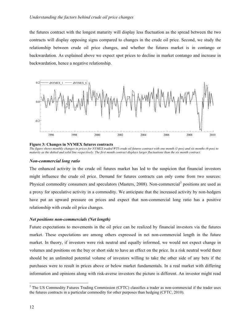
the futures contract with the longest maturity will display less fluctuation as the spread between the two

contracts will display opposing signs compared to changes in the crude oil price. Second, we study the

relationship between crude oil price changes, and whether the futures market is in contango or

backwardation. As explained above we expect spot prices to decline in market contango and increase in

backwardation, hence a negative relationship.

Figure 3: Changes in NYMEX futures contracts The figure shows monthly changes in prices for NYMEX traded WTI crude oil futures contract with one month (1-pos) and six months (6-pos) to maturity as the dotted and solid line respectively. The first month contract displays larger fluctuations than the six month contract.

Non-commercial long ratio

The enhanced activity in the crude oil futures market has led to the suspicion that financial investors

might influence the crude oil price. Demand for futures contracts can only come from two sources:

Physical commodity consumers and speculators (Masters, 2008). Non-commercial3 positions are used as

a proxy for speculative activity in a commodity. We anticipate that the increased activity by non-hedgers

have put an upward pressure on prices and expect that non-commercial long ratio has a positive

relationship with crude oil price changes.

Net positions non-commercials (Net length)

Future expectations to movements in the oil price can be realized by financial investors via the futures

market. These expectations are among others expressed in net non-commercial length in the future

market. In theory, if investors were risk neutral and equally informed, we would not expect change in

volumes and positions on the buy or short side to have an effect on the price. In a risk neutral world there

should be an unlimited potential volume of investors willing to take the other side of any bets if the

purchases were to result in prices above or below market fundamentals. In a real market with differing

information and opinions along with risk-averse investors the picture is different. An investor might read

3 The US Commodity Futures Trading Commission (CFTC) classifies a trader as non-commercial if the trader uses the futures contracts in a particular commodity for other purposes than hedging (CFTC, 2010).

dNYMEX_1 dNYMEX_6

1996 1998 2000 2002 2004 2006 2008 2010

-0.2

0.0

0.2 dNYMEX_1 dNYMEX_6


13

the other investor’s willingness to buy a large volume of contracts as a possible signal that they know

something she does not. Financial micro-structure theory (Dufour & Engle, 2000) predicts that a large

volume of purchases (sells) may well cause the price to increase (decrease), at least temporarily, until the

investor can verify the fundamentals.

We will investigate two relationships between net positions and crude oil prices. First we study the

relationship between changes in net positions versus changes in the crude oil price. We expect that

changes in net positions will affect oil prices positively, since an increased number of long positions will

increase demand for crude oil. Second we inspect the relationship between oil price changes and the

actual net position held by non-commercial traders each month. We expect that when the market is net

long this will put an upward pressure on prices. Hence, we expect a positive relationship between net

positions and crude prices.


14

2.6 Summary of hypotheses

Table 1 summarizes all variables, variable names, their meaning, and expected signs of corresponding

coefficients discussed in this section. The discussion of hypotheses for the different variables show that it

is difficult to draw conclusions based on their signs and values. This is the first justification of the state-

space approach where we can identify how they behave differently over time due to the general condition

in the economy.

Table 1: Summary of hypotheses4 Category Variable Description Sign Demand D dD_wgrowth Change in world economic growth + dD_exch$ Change in the real effective exchange rate - Supply S dS_stock Change in days of stock cover (OECD) +/- dS_rigu Change in world rig utilization excl. Jack-ups Gulf of Mexico + dS_rigu_GoM Change in rig utilization Jack-ups Gulf of Mexico + dS_vlcc Change in world Tanker charter rates (+) dS_refu Change in refinery utilization +/- OPEC dOPEC_sparecap Change in OPEC spare capacity level - dOPEC_quota Change in OPEC production quotas - dOPEC_cheat Change in OPEC cheat on production quoats - Futures Market Variables F F_cont(level) Market Contango/Backwardation level - dF_cont Change in market Contango/Backwardation level - dF_oi Change in non-commercial long ratio + F_netl(level) Net length for non-commercial positions + dF_netl Change in net length for non-commercial positions + Dummy Variables (Special events) D Dumm_event(+) Dummy for positive events affecting demand and negative for

supply, such as hurricanes. +

Dumm_event(-) Dummy for negative events affecting demand and positive for supply, such as terrorist attacks and financial crisis.

-

The table lists all variables, notation and description used to describe crude oil prices, as well as their hypothetical impact. Signs in parentheses are variables not expected to be significant during the whole time period (as explained above). dSrigu_GoM is described in the Data description in the next section..

4 The reason for utilizing transformed data series is argued in section 3.2.


15

3. Data

3.1 Data description

We collect monthly or monthly average data for each of the factors outlined in the previous section for the

time period from January 1995 to December 2009. The choice of sample period is determined by

economic considerations and data constraints. The data are collected from various sources and

transformed to give the most efficient and correct picture to each of the hypothesis. Figure 4 plots the

selected data series.

3.1.1 Dependent variable

The dependent variable is the world crude price. To avoid local differences in the United States WTI and

European Brent market we use the average price between the two markers, traded in US Dollar per barrel,

to construct a basket price, P_crude. The two markers are chosen since they represent the most common

benchmarks and are the two most traded crudes on the future exchanges.

3.1.2 Explanatory variables

Demand

The weighted world production index, D_wgrowth, by the Netherlands Bureau for Economic Policy

Analysis (CPB) gathered from Reuters Ecowin is utilized as a proxy for world economic growth, in the

same manner as Williams (2008). There is no reliable data available on world GDP, and the country

specific data are only reported quarterly.

By utilizing the US Dollar/OECD real exchange rate, D_Exch$, two desirable properties arise. First, the

real exchange rate adjusts for inflation and second, the US Dollar is compared against a pool of OECD

currencies, thus encompassing a clearer picture of the US Dollar value relative to the rest of the industrial

world’s currencies. The OECD countries constitute the biggest part of the world economy and other large

influential economies like China have their currencies pegged to the US Dollar. We thereby consider

D_Exch$ to be a satisfying measure on the total currency effects in the crude oil market. Figure 4 shows a

depreciation of the dollar since 2002.

Supply

Days of stock cover, S_Stock, is calculated utilizing monthly stock data and consumption data for the

OECD countries from Energy Information Administration (EIA).


16

___

tt

t

OECD StockS StockOECD Production

=

The OECD countries consume over 50 percent of the crude oil produced (EIA), and should work as a

desirable proxy for the total stock cover worldwide. Figure 4 indicates seasonality in the S_Stock data,

with low levels around January, and high levels around June each year. This seasonality stems from

natural cycles in the world oil demand. We choose not to adjust for seasonality in our data as there are a

number of issues with doing so, including loss of explanatory power.

Rig utilization, S_rigu, is gathered from ODS-Petrodata for jack-up rigs and floaters (semi-submersibles

and drill ships). We have split the utilization rates for jack-ups positioned in the US Gulf of Mexico and

those elsewhere. This is done because this market is more mature and based on spot prices, which should

react and reflect market conditions and reactions to crude prices stronger than other markets.

World tanker rates, F_vlcc, are collected from Reuters EcoWin. The rates are measured in thousand US

Dollars per day. The crude tanker market consists of many ship types, however the largest segment is the

Very Large Crude Carriers (VLLC), and we will use these rates. Figure 4 shows that the VLCC rates are

considerably more volatile in the latter half of the sample, which reflects uncertainty and periodically

imbalance in the global tanker market.

To evaluate the effect of conditions in the refining sector on crude oil prices, we collect data on US

refinery utilization rates, S_refu, in the same manner as Dèes et al. (2008). We collect 4 week averages

from the EIA. Global data would be preferred, but only US data are available. Nonetheless, US refinery

utilization should be satisfactory since it represents about 20 percent of world capacity in 2006

(Kaufmann R. , Dèes, Gasteuil, & Mann, 2008). The market for refined petroleum products is global and

it is unlikely that utilization rates in one part of the world will differ dramatically from other parts. As

long as one can transport refined petroleum products, it is improbable that US refinery utilization rates

will increase while other countries’ rates will decline significantly. If the greatest shortage of refining

capacity occurs in the US, then US refinery rates are the relevant measure because it would reflect

conditions at the margin, which by definition, determine prices (Kaufmann, Dees, Gasteuil, & Mann,

2008). The last notion is based on results which indicate that the price crude oil produced in geographical

different parts of the world co-integrate (Bacheimer & Griffin, 2006).

OPEC data on production, capacity and quota is gathered from the EIA and PIRA Energy Group (PIRA).

OPEC_quota is the OPEC production quota in million barrels per day (mbd).


17

The OPEC spare capacity, OPEC_sparecap, and is collected from the EIA. It is calculated as the

difference between capacity and production, measured in mbd;

_ _ _t t tOPEC sparecap OPEC capacity OPEC production= −

OPEC production quotas, OPEC_quota, are collected from PIRA. The extent to which the OPEC

countries cheat on their production quotas, OPEC_cheat, is calculated as the difference between

production quota and actual production (measured in mbd);

_ _ _t t tOPEC cheat OPEC quota OPEC production= −

Futures market

The contango and backwardation market condition is measured by compiling monthly averages on the

near month (1-pos) contract and the six month (6-pos) contract for WTI traded on NYMEX. The spread

between the two price series is then used to determine the market position, F_cont; that is if the slope of

the forward curve.

t t tF_cont = NYMEX(6 - pos) - NYMEX(1- pos)

Figure 4 shows that prior to 2005 the market was mainly in backwardation, which agrees with

Litzenberger & Rabinowitz’s studies (1995). However, after 2005 the market has mainly been in

contango. According to our hypothesis, this implies that the market has had an optimistic outlook on the

future crude oil price over the last 5 years.

The percentage of non-commercial open interest, F_oi, is collected from the Commitments of Traders

(COT) report reported by the CFTC. It is calculated as the proportion of long positions held by non-

commercial traders and is calculated as:

_ t tt

t t

NCL NCSPF oiOI NRLP

+=

−

where, NCLt is the non-commercial long positions, NCSPt the non-commercial spread positions, OIt the

total positions of all traders and NRLPt the Non-reportable long positions for every month, t. We subtract

the non-reportable positions since the numbers consists of smaller positions held by both commercial and

non-commercial traders. Figure 4 shows that the percentage of non-commercial open interest has

increased considerably during the sample period. An interesting observation is that the ratio did not

decrease in connection with the financial crisis.


18

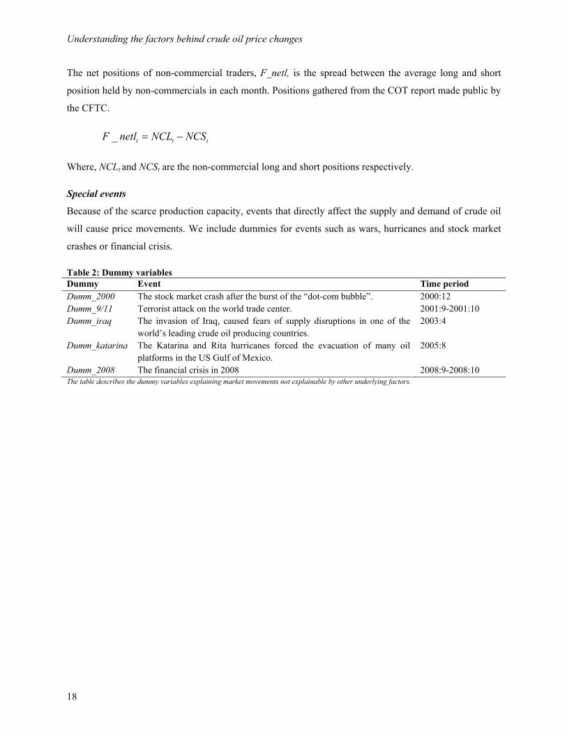
The net positions of non-commercial traders, F_netl, is the spread between the average long and short

position held by non-commercials in each month. Positions gathered from the COT report made public by

the CFTC.

_ t t tF netl NCL NCS= −

Where, NCLt and NCSt are the non-commercial long and short positions respectively.

Special events

Because of the scarce production capacity, events that directly affect the supply and demand of crude oil

will cause price movements. We include dummies for events such as wars, hurricanes and stock market

crashes or financial crisis.

Table 2: Dummy variables Dummy Event Time period Dumm_2000 The stock market crash after the burst of the “dot-com bubble”. 2000:12 Dumm_9/11 Terrorist attack on the world trade center. 2001:9-2001:10 Dumm_iraq The invasion of Iraq, caused fears of supply disruptions in one of the

world’s leading crude oil producing countries. 2003:4

Dumm_katarina The Katarina and Rita hurricanes forced the evacuation of many oil platforms in the US Gulf of Mexico.

2005:8

Dumm_2008 The financial crisis in 2008 2008:9-2008:10 The table describes the dummy variables explaining market movements not explainable by other underlying factors.


19

Figure 4: Time series plot Development of all time series from 1995:1 to 2009:12, Crude oil price basket price is listed in US Dollars per barrel. World growth is a weighted production index (2000=100). The US Dollar real effective exchange rate is an index describing the dollar cost of buying a unit of an index composed of an index of a pool of OECD currencies, adjusted for inflation. Rig utilization for the world and for jack-ups in the US Gulf of Mexico is the ratio of working rigs versus the total available market. Days of stock cover is the number of days available in OECD crude stocks. World tanker rates are given in USD. OPEC spare production capacity, quota, and cheat on quotas are given in thousand barrels per day. Refinery utilization is the ratio of occupied versus available capacity in the US refinery sector. Contango/Backwardation is the spread between the 6 month and first delivery month contract on NYMEX in US Dollars per barrel. Non-commercial long ratio of open interest is given as a ratio. Non-commercial net length is the spread between long and short positions given in number of contracts on NYMEX.

P_crude

1995 2000 2005 2010

50

100

150P_crude D-wgrowth

1995 2000 2005 2010

100

120

140D-wgrowth

D_Exch$

1995 2000 2005 2010

90

100

110

120D_Exch$ S_rigu

1995 2000 2005 2010

80

90

100S_rigu

S_rigu_GoM

1995 2000 2005 2010

50

75

100 S_rigu_GoM

S_Stock

1995 2000 2005 2010

80

90

100S_Stock

S_vlcc

1995 2000 2005 2010

100

200S_vlcc OPEC_sparecap

1995 2000 2005 2010

2500

5000

7500OPEC_sparecap

OPEC_quota

1995 2000 2005 2010

22500

25000

OPEC_quota OPEC_cheat

1995 2000 2005 2010

0

2000

4000OPEC_cheat

S_refu

1995 2000 2005 2010

80

90

100S_refu F_cont

1995 2000 2005 2010

0

10F_cont

F_p.oi

1995 2000 2005 2010

0.1

0.2

0.3F_p.oi F_netl

1995 2000 2005 2010

0

100000

200000F_netl


20

3.2 Descriptive statistics

Descriptive statistics for the data series is presented in Table 3. The table shows the basic features of the

series, and presents test results for normality and stationarity. The explanatory variables are also checked

for multicollinearity. For a description of the statistical concepts used we refer to Appendix A.4.

The Jarque-Bera test reveals that the data series are generally non-normally distributed, as most of the

series are skewed to the right and have low kurtosis. The Augmented Dickey-Fuller (ADF) test is used to

test the data series for stationarity at 5 and 1 percent significance level. State-space modeling in itself does

not require stationary time series, but since our model selection process is based on ordinary linear

regression we need to fulfill this assumption. In ordinary linear regression use of non-stationary series

strongly influence the behavior and properties of the final state-space model. Potential hazards with use of

non-stationary series could, in our case, be infinite persistence of shocks and spurious relationships.

Thereby, we would not be able to draw any valid inferences. The ADF-procedure tests the null hypothesis

that the data series is non-stationary against the alternative hypothesis that the data series is stationary. As

shown in Table 3, most of the time series are found to be non-stationary, as the test statistic fails to reject

the null hypothesis. This is not surprising, since real prices and levels often contain a stochastic trend.

The correlation-matrix for the explanatory variables, attached in Appendix A.2, indicates that the problem

of multicollinearity is present for some of the variables in the data series and should be taken into

account.

The presence of non-stationarity and multicollinearity in our variables indicates a need to consider either

the data or the method we intend to use further. A possible solution to the non-stationary problem is based

on co-integrated relationships among the variables, as applied by Kaufmann et al. (2004) and Möbert

(2007). Engle & Granger’s (1987) two-step method is applied to determine if two (or more) variables co-

integrate, but due to our large number of non-stationary explanatory variables the approach fails to supply

an adequate specification. Instead of estimating an Error Correction Model (ECM), we transform the data

series by differentiation. One issue with differentiating the data is that some long-term statistical

equilibrium relations between the variables will be lost. Another solution to the problem is to study a

State-Space Error Correction Model (SSECM) (Ribarits & Hanzon, 2009), but the methodology is new

and is to our knowledge not utilized in the literature.

The data are transformed by the natural logarithm and calculate the first order difference (denoted

log_diff) to avoid problems with non-stationary means and level differences.


21

1

t

t

Plog_diff lnP−

=

Descriptive statistics for log_diff series are represented in Table 3. All of the log_diff series reject the null

hypothesis that the data are non-stationary at 1 percent significance level, implying that that all series are

stationary. The correlation-matrix (Table 9 in appendix) of the transformed data shows no signs of having

potentially harmful correlations. These findings are desirable for the later model specification. Time plots

of the log_diff data for the time period from January 1st 1995 to December 31st 2009 are presented in

Figure 5.

The purpose of this paper is to study the time-varying coefficients affecting the crude oil market.

Correlation matrices are studied with the purpose of study possible problems with multicollinearity, but

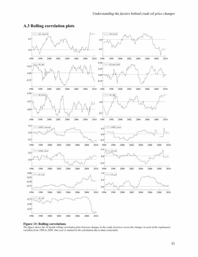
we also want to study how the factors correlate with the crude oil price during the time period. Figure 13

in Appendix A.3 shows the 24 month rolling correlation between the crude oil price and each of the

explanatory variables during the time period. We observe that the relationship varies throughout the time

period studied and supports our reasoning for applying a time-varying model to study the dynamic effects

in the crude oil market. We will refer back to Figure 13 when analyzing the results from our model.


22

Figure 5: Plot of transformed data Logarthmic differences of the data series from 1995:1 to 2009:12. P_crude is the change in the crude oil basket price listed in US Dollars per barrel. World growth is a weighted production index (2000=100). The US Dollar real effective exchange rate is an index describing the dollar cost of buying a unit of an index composed of an index of a pool of OECD currencies, adjusted for inflation. Rig utilization for the world and for jack-ups in the US Gulf of Mexico is the ratio of working rigs versus the total available market. Days of stock cover is the number of days available in OECD crude stocks. World tanker rates are given in USD. OPEC spare production capacity, quota, and cheat on quotas are given in thousand barrels per day. Refinery utilization is the ratio of occupied versus available capacity in the US refinery sector. Contango/Backwardation is the spread between the 6 month and first delivery month contract on NYMEX in US Dollars per barrel. Non-commercial long ratio of open interest is given as a ratio. Non-commercial net length is the spread between long and short positions given in number of contracts on NYMEX.

dP_crude

1995 2000 2005 2010

-0.2

0.0

0.2dP_crude dD_wgrowth

1995 2000 2005 2010

-0.02

0.00

0.02dD_wgrowth

dD_Exch$

1995 2000 2005 2010

0.00

0.05dD_Exch$ dS_rigu

1995 2000 2005 2010

-0.025

0.000

0.025 dS_rigu

dS_rigu_GoM

1995 2000 2005 2010

-0.2

0.0

0.2dS_rigu_GoM dS_Stock

1995 2000 2005 2010

-0.1

0.0

0.1dS_Stock

dS_vlcc

1995 2000 2005 2010

-0.5

0.0

0.5

1.0dS_vlcc dOPEC_sparecap

1995 2000 2005 2010

-0.5

0.0

0.5 dOPEC_sparecap

dOPEC_quota

1995 2000 2005 2010

-0.05

0.00

0.05

0.10dOPEC_quota dOPEC_cheat

1995 2000 2005 2010

-0.25

0.00

0.25

0.50dOPEC_cheat

dS_refu

1995 2000 2005 2010

-0.1

0.0

0.1dS_refu dF_cont

1995 2000 2005 2010

-0.025

0.000

0.025

0.050dF_cont

dF_p.oi

1995 2000 2005 2010

-0.025

0.000

0.025dF_p.oi dF_netl

1995 2000 2005 2010

-0.25

0.00

0.25 dF_netl

Und

erst

andi

ng th

e fa

ctor

s beh

ind

crud

e oi

l pri

ce c

hang

es

23

Tab

le 3

: Des

crip

tive

stat

isitc

s

Th

e to

p ta

ble

show

s th

e de

scri

ptiv

e st

atis

tics

for

the

indi

vidu

al ti

me

seri

es a

nd b

otto

m ta

ble

for

the

tran

sfor

med

dat

a se

ries

(log

_diff

). Th

e Ja

rque

-Ber

a te

st s

tatis

tic is

the

test

for

norm

ality

, and

AD

F is

th

e Au

gmen

ted

Dic

key

Fulle

r uni

t roo

t tes

t. **

and

* in

dica

tes s

tatis

tical

sign

ifica

nce

at th

e 1

perc

ent a

nd 5

per

cent

sign

ifica

nce

leve

l res

pect

ivel

y.

P_cr

ude

D-w

grow

thD

_exc

h$S_

rigu

S_ri

gu_G

oMS_

stoc

kS_

vlcc

OPE

C_

spar

ecap

OPE

C_q

uota

OPE

C_c

heat

S_re

fuF_

cont

F_p.

oiF_

netl

Mea

n39

.611

105.

447

100.

187

87.1

0176

.771

83.4

0670

.160

2895

.667

2372

8.78

342

0.61

190

.903

-0.0

470.

168

3261

3.76

0St

anda

rd E

rror

1.94

11.

149

0.54

40.

471

1.05

40.

354

2.38

510

8.78

514

0.00

860

.828

0.32

20.

211

0.00

539

05.0

66M

edia

n28

.593

101.

520

100.

620

87.8

3877

.805

82.6

1360

.348

2830

.000

2310

7.00

030

4.45

991

.550

-0.4

970.

156

2939

0.62

5St

anda

rd D

evia

tion

26.0

3615

.422

7.29

86.

318

14.1

354.

754

31.9

9914

59.5

0918

78.4

0181

6.09

34.

318

2.83

30.

071

5239

1.95

9K

urto

sis

1.65

9-1

.107

-0.7

58-0

.630

2.58

41.

053

2.96

0-0

.440

-1.1

431.

042

0.83

41.

743

-1.2

090.

171

Skew

ness

1.38

40.

313

0.11

2-0

.368

-1.2

690.

790

1.42

00.

497

0.30

60.

555

-0.7

361.

012

0.39

40.

489

Rang

e12

2.81

552

.560

29.0

8024

.770

70.5

8026

.847

200.

290

6230

.000

5974

.000

5174

.000

25.7

0017

.225

0.23

027

2635

.250

Min

imum

10.5

2882

.140

85.9

4071

.800

26.1

3072

.433

21.8

6971

0.00

020

575.

000

-146

1.00

073

.700

-5.6

510.

072

-814

45.7

50M

axim

um13

3.34

313

4.70

011

5.02

096

.570

96.7

1099

.281

222.

159

6940

.000

2654

9.00

037

13.0

0099

.400

11.5

740.

302

1911

89.5

00

Jarq

ue-B

era

75.2

70

[0.0

000]

**12

.116

[0

.002

3]**

4.81

51

[0.0

900]

7.

1182

[0

.028

5]*

93.5

70

[0.0

000]

**25

.747

[0

.000

0]**

120.

20

[0.0

000]

**8.

8840

[0

.011

8]*

12.5

90

[0.0

018]

**16

.305

[0

.000

3]**

20.5

07

[0.0

000]

**50

.882

[0

.000

0]**

15.4

43

[0.0

004]

**7.

1937

[0

.027

4]*

ADF

-1.2

21-0

.680

-1.4

16-2

.457

-1.4

480.

342

-4.2

25**

-1.8

-1.9

31-3

.751

**0.

902

-2.8

59-0

.409

-3.6

05**

Cou

nt18

018

018

018

018

018

018

018

018

018

018

018

018

018

0

dP_c

rude

dD-w

grow

thdD

_exc

h$dS

_rig

uS_

rigu

_GoM

dS_s

tock

dS_v

lcc

dOPE

C_

spar

ecap

dOPE

C_q

uota

dOPE

C_c

heat

dS_r

efu

dF_c

ont

dF_p

.oi

dF_n

etl

Mea

n0.

0083

0.00

250.

0001

0.00

04-0

.004

30.

0008

-0.0

017

0.00

310.

0000

0.00

16-0

.000

80.

0002

0.00

090.

0024

Stan

dard

Err

or0.

0067

0.00

050.

0009

0.00

080.

0041

0.00

270.

0164

0.01

350.

0014

0.00

950.

0023

0.00

080.

0010

0.00

73M

edia

n0.

0230

0.00

360.

0000

0.00

110.

0003

-0.0

004

-0.0

082

0.00

000.

0000

0.00

84-0

.001

1-0

.000

50.

0013

0.00

14St

anda

rd D

evia

tion

0.08

970.

0062

0.01

270.

0109

0.05

440.

0360

0.21

980.

1816

0.01

920.

1272

0.03

150.

0113

0.01

290.

0978

Kur

tosi

s1.

3262

9.17

452.

0626

1.64

738.

9029

-0.0

530

2.37

078.

5260

10.3

230

2.32

316.

6722

2.04

680.

7242

0.17

99Sk

ewne

ss-0

.839

2-2

.095

10.

1456

-0.1

366

-1.9

946

0.06

880.

3261

-0.8

951

0.33

40-0

.547

2-0

.576

10.

0314

-0.2

568

-0.1

175

Rang

e0.

5058

0.05

020.

0979

0.07

340.

4219

0.20

141.

6717

1.56

080.

1821

0.85

840.

3003

0.08

460.

0765

0.58

00M

inim

um-0

.309

3-0

.030

7-0

.041

6-0

.038

0-0

.300

0-0

.101

5-0

.816

5-0

.943

1-0

.087

7-0

.475

7-0

.164

8-0

.042

1-0

.040

9-0

.320

2M

axim

um0.

1965

0.01

940.

0563

0.03

540.

1219

0.09

990.

8552

0.61

770.

0943

0.38

270.

1356

0.04

260.

0356

0.25

98

Jarq

ue-B

era

32.6

29

[0.0

000]

**71

8.16

[0

.000

0]**

29.8

61

[0.0

000]

**19

.020

[0

.000

1]**

675.

46

[0.0

000]

**0.

1939

8 [0

.907

6]41

.866

[0

.000

0]**

489.

08

[0.0

000]

**75

3.06

[0

.000

0]**

46.0

02

[0.0

000]

**32

2.63

[0

.000

0]**

28.9

69

[0.0

000]

**5.

3624

[0

.068

5]0.

5570

2 [0

.756

9]AD

F-1

0.14

**-4

.867

**-8

.718

**-3

.751

** -7

.924

**-3

.847

**-1

3.40

**-1

0.91

**-1

1.75

**-9

.680

**-4

.987

**-1

1.47

**-9

.810

**-6

.984

**

Cou

nt18

018

018

018

018

018

018

018

018

018

018

018

018

018

0


24

4. Methodology The empirical methodology aims to determine significant factors influencing the oil price and to

investigate their change over time. To identify the factors we want to include in the time-varying model,

we employ a classical linear regression model (CLRM) with oil price return as the dependent variable and

the discussed factors as explanatory variables. The following specification applies;

,1

k

t i i t ti

y Xα β ε=

= + +∑ 2(0, )t NID εε σ∼ (1)

where α is a constant, Xi is the data series of the explanatory variable i, βi is the beta coefficient for the

explanatory variable i, including dummies, and the residuals εt are Gaussian white noise.

The general unrestricted model (GUM) gives an unlimited number of combinations of variables and lags.

Therefore several techniques are applied to indentify the most efficient and parsimonious model. The

Autometrics function in the Oxmetrics software, economic theory and related research are utilized to

identify the significant variables and most significant lags. Diagnostic tests are performed to reveal

whether the models fulfill the assumptions related to an Ordinary Least Squares (OLS) regression model.

Detailed descriptions of the software and statistical tests used are attached in Appendix A.4.

4.1 Parameter stability of the linear regression

To evaluate the stability of the parameters in the model we employ a Chow test. The test splits the data

into two sub-periods and estimate the regression over the whole period (restricted regression) and then for

the two sub-periods separately (unrestricted regressions). Residual sum of squares (RSS) is obtained for

each regression, and thereof it is performed an F-test based on the test statistic;

1 2

1 2

( ) 2_ RSS RSS RSS T ktest statisticRSS RSS k− + −

= ×+

where T is the number of observations and k is the number of independent variables in each unrestricted

regression. Hence, the test checks whether the residual sum of squares for the whole sample (RSS) is

larger than the sums of squares for the two sub-samples ( 1 2RSS RSS+ ). As usual with an F-test, if the

value of the test-statistics is greater than the critical value from the F-distribution, which is F(k, T-2k), we

reject the null hypothesis that the parameters are stable over time.


25

4.2 Estimate model with time-varying parameters

To investigate further how the different factor coefficients behave over time we will apply a state space

approach. We will base our theoretical framework on Commandeur & Koopman (2007) and Tsay (2005),

with Wei (2006) and Hamilton (1994) as supporting literature. The deterministic regression model (1) is

expanded to a state space model by introducing a level component, µt, which is allowed to vary over time.

The level component can be conceived of as an equivalent of the intercept in the ordinary linear

regression, but in contrast this component applies only locally at each time point (Commandeur &

Koopman, 2007). To model the level component we are adding an equation representing the state of the

level component in the model. Similarly, we let the beta values, βt, for each of the explanatory variables

vary over time. The modeling of k explanatory variables requires k additional state equations. We then

have the following linear Gaussian local level state space model, consisting of an observation equation (2)

and several state equations (3), (4).

, ,1

k

t t i t i t ti

y Xμ β ε=

= + +∑ 2(0, )t NID εε σ∼ (2)

1t t tAμ μ η+ = + 2(0, )t NID ηη σ∼

(3)

, 1 ,i t i t tβ β τ+ = + 2(0, )t NID ττ σ∼ (4)

We let εt, ηt, τt be independent Gaussian white noise series. The variables µt and βi,t are the state of the

system at time t and are not directly observed, while yt is the observed version of µt and βt with added

noise. The first equation (2), known as the observation equation, therefore provides a link between the

data yt and the state. The latter equations (3), (4), the state equations, govern the time evolution of the

state variables. Hence, we have one equation which relates the crude oil price to the changes in the

driving factors, while the other equations model the effects dynamically. The model shows the

unobserved dynamic process at different points in time, and we can observe the stochastic behavior of the

level and the slopes of the model.

The time-varying coefficients are estimated using Kalman filtering (Kalman, 1960). This technique lets

the model update the state variables recursively by Bayesian optimization as we work through the time

series data. We let Ft = {y1,….,yt} be the information available at time t. Knowing the conditional

distribution of the state variables given Ft-1 and the new data yt, we can obtain the conditional distribution

of state variables given Ft. Recursive estimates of the state variables and their variance are made by the

observation equations. Starting from the initial estimates, the observation equation updates to prior values


26

of the variables are updated in each time step. Once the new data yt+1 is included, the procedure is

repeated to update knowledge of next observation of the state variables (Tsay, 2005).

We can expand the derived model further by adding trend- and seasonality components. Thus, we obtain

the following final state space model;

, ,1

k

t t t i t i t ti

y Xμ γ β ε=

= + + +∑ 2(0, )t NID εε σ∼ (5)

1t t t tAμ μ υ η+ = + + 2(0, )t NID ηη σ∼

(6)

, 1 ,i t i t tβ β τ+ = + 2(0, )t NID ττ σ∼ (4)

1 ,t i t tυ υ ζ+ = +

2(0, )t NID ζζ σ∼

(7)

, 1 ,i t i t tγ γ ϕ+ = +

2(0, )t NID ϕϕ σ∼

(8)

The level-, slope- and seasonal components can be set to be fixed, stochastic or omitted. Each of the

regression coefficients, the betas, can be set to be fixed, random walk (Markov process) or smoothing

spline. By allowing the regression coefficients to vary over time in a random walk specification, we can

observe how they behave in accordance to market fundamentals. Smoothing spline is a method of fitting a

smooth curve to a set of noisy observations, and is useful to illustrate the overall development of the

coefficients over time. The random walk specification (4) is defined in the model above, while the

alternative smoothing spline (9) specification is defined as:

, , 1i t i t tβ β τ−Δ =Δ +

2(0, )t NID ττ σ∼ (9)

To determine which factors of the regression that show a significant influence on the crude oil price, we

test different versions of state space model in Oxmetric STAMP (Structural Time Series Analyser,

Modeller and Predictor). We set all the regression coefficients fixed, whilst testing for the different

specifications for the level-, slope- and seasonal components. Subsequently we perform tests where we let

the regression coefficients fluctuate over time as a random walk process, first one coefficient at a time and

finally all the coefficients simultaneously.

We evaluate the different models by using the Akaike Information Criterion (AIC) (Akaike, 1973). The

criterion compensates for the number of estimated parameters, thus allowing for a fair comparison


27

between models involving different number of parameters. The AIC is described further in Appendix A.4.

Additionally, several diagnostic tests are performed to reveal whether the residuals of the model fulfill the

requirements of a linear Gaussian model, which is no signs of heteroscedasticity, autocorrelation, non-

normality, or other biasing signs. The property of no autocorrelation is particular important. The test

descriptions are attached in the Appendix A.4. Performing these tests are crucial in order to validate

whether our conclusions are statistical adequate.


28

5. Empirical results

5.1 Model selection

From a general unrestricted model, including all explanatory variables and lagged variables, we revealed

the most significant factors and appropriate lags in the OxMetrics 6.0 software. We intended to avoid high

lags, if not there were clear and reasonable economic reasons for including them. The final model

selection is based on a number of criteria described in the theoretical framework and Appendix A.4. To

avoid problems with misspecifications, large outliers and heteroscedasticity in the residuals we add the

dummies found significant at the 1 percent significance level. The dummies represent special events

during the time period that have affected price movements. One event during the time period is found to

be significant. The financial crisis in 2008 and the market crash that followed caused crude oil price

movements that are not explainable by any of our covariates.

Following the steps presented in the theoretical framework, the best model was identified by fixing the

coefficients of the explanatory variables, and evaluate different models based on their AIC. We tested 18

different models by allowing the level-, slope- and seasonal components to be fixed, stochastic or omitted.

The model with a fixed level and slope, and an omitted seasonal component gave us the best goodness of

fit by evaluating AIC. Based on our model selection process we are left with our final model shown in

Table 4.

Table 4: Linear regression model Variable Coefficient Std.Error t-value t-prob dD_wgrowth 3.5754 0.7777 4.600 0.0000 *** dS_rigu_1 0.7040 0.3951 1.780 0.0766 * dS_Stock 0.2161 0.1192 1.810 0.0717 * dOPEC_sparecap -0.0386 0.0239 -1.690 0.0922 * dOPEC_quota -0.6424 0.2334 -2.750 0.0066 *** dS_refu_2 0.2396 0.1354 1.770 0.0787 * dF_cont -3.3457 0.4048 -8.270 0.0000 *** dF_netl 0.3530 0.0453 7.800 0.0000 *** dumm_2008 -0.1542 0.0414 -3.720 0.0003 ***

2R 0.6604 H-test(55) 1.5643 DW 1.6064 RESET23 1.8718 Normality(2) 9.0082** RSS 0.4556 AIC -5.7644 The table shows the final model with each variable and its significant lag. ***, **, * indicates that the factors are significant at 1 percent, 5 percent and 10 percent significance level respectively.


29

Changes in economic growth, OPEC production quotas, contango level and net length positions held by

non-commercials are all significant at a 1 percent significance level. Rig utilization at the first lag, days of

stock cover, OPEC spare production capacity and refinery utilization at the second lag are significant at

the 10 percent significance level5. The test summary in Table 4 shows that the goodness of fit (R2) is 66

percent, which is about the same result achieved by Möbert’s (2007) various linear regression models.

The H-test for heteroscedasticity does not reject the null hypothesis that the residuals are homoscedastic

and the RESET23 test shows no signs of misspecification and non-linearities in the model. The Durbin –

Watson DW statistic does indicate some signs of positive serial correlation, but the test-statistic is not

significantly different from 2 to reject the null hypothesis. Finally, the Jarque-Bera Normality test rejects

the null hypothesis that the residuals are normally distributed. This could be caused by outliers, but we

choose not to correct for this by adding dummies and loose the explanatory power of the covariates in the

state-space model. This should be solved by the state-space model specifications and we will study this

closely in the residuals from our time-varying model.

5.1.1 Parameter stability

To evaluate the parameter stability we employed the Chow test described in the theoretical framework. As

a simple test we divided our dataset into two periods, first period from 1995 to 2003 and second period

from 2004 to 2009. The division point is based on the large increase in crude oil price from 2004. Using

the linear regression model defined above we obtain the residual sum of squares for both time periods.

The test statistic is above the critical value at 1 percent significance level in the F-distribution, and we

reject the null hypothesis that the parameters are stable over time. To fully evaluate the stability of the

parameters, and identify possible break-points, we employ the recursive tests offered by the Oxmetrics

software. The 1-step (1up CHOWs) in Figure 6 shows the parameter stability test for each time step.

There are some serious outliers from the critical value at 1 percent significance level, and we observe that

the outliers are more frequent after 2005. This is in accordance with the simple two-period Chow test we

performed above. The break-point (Ndn CHOWs) test rejects the null hypothesis that the parameters are

stable for almost the whole sample. In Figure 6 the parameters seem to be stable during the financial

crisis, but this is actually caused by the dummy which is included in the regression to fulfill the

assumptions for the regression. The 1-step residual plot (Res1 Step) shows some outliers from the 2

standard-error region, which could be associated with coefficient changes. We also observe that the 2

standard-error region become wider during the sample, indicating more instability. The parameter

5 We choose to include variables found significant at the 10 percent significance level since the linear model is a selection process for the time-varying model, and the significance of each coefficient will vary through time.


30

instability suggests that there are some structural breaks during the period and to explore these a model

with time-varying parameters is more appropriate than a linear model.

Figure 6: Chow test graphics Residual 1-step plot, 1-step Chow test and break-point Chow test for the final linear regression. The tests indicate unstable parameters.

Res1Step

1996 1997 1998 1999 2000 2001 2002 2003 2004 2005 2006 2007 2008 2009 2010

-0.1

0.0

0.1

0.2Res1Step

1up CHOWs 1%

1996 1997 1998 1999 2000 2001 2002 2003 2004 2005 2006 2007 2008 2009 2010

1

2

1up CHOWs 1%

Ndn CHOWs 1%

1996 1997 1998 1999 2000 2001 2002 2003 2004 2005 2006 2007 2008 2009 2010

1

2Ndn CHOWs 1%


31

5.2 Time-varying coefficients

Figure 7 illustrates each of the significant factors’ time varying influence on the crude oil price changes.

The model where the beta coefficients follow a random walk performed better than the smoothing spline

alternative, when evaluating the models by the AIC. When the coefficients follow a random walk over

the period we can examine the unobserved dynamics in the linear regression model. It should be noted

that the behavior of each coefficient is determined given the presence of the remaining time varying

coefficients at any given time. As a comparison we refer to the Appendix A.1 where each explanatory

factor’s time varying influence on the crude oil price is illustrated, independent of the other factors.

Figure 7: Time-varying beta coefficients The figure shows the random-walk time plots for the coefficients of each of the significant underlying factors in the model in the time period from 1995 to 2009.

Table 5: Summary of test statistics for the state-space model Test summary DW 1.6972 Ljung-Box Q(11) 16.025 H-test(55) 1.6456 Normality(2) 2.5124 The Durbin-Watson test for residual autocorrelation, the Ljung-Box test statistic for residual autocorrelation, the Heteroscedastic test statistic

and the Jarque-Bera Normality test statistic. ***, ** indicates that the factors are significant at 1 percent amd 5 percent significance level

respectively.

dP_crude-RW-coef dD_wgrowth

1995 2000 2005 2010

2.5

5.0dP_crude-RW-coef dD_wgrowth dP_crude-RW-coef dS_rigu_1

1995 2000 2005 2010

1

2dP_crude-RW-coef dS_rigu_1

dP_crude-RW-coef dS_Stock

1995 2000 2005 2010

0.22

0.24dP_crude-RW-coef dS_Stock dP_crude-RW-coef dOPEC_sparecap

1995 2000 2005 2010

-0.2

0.0dP_crude-RW-coef dOPEC_sparecap

dP_crude-RW-coef dOPEC_quota

1995 2000 2005 2010

-0.5

-0.4

-0.3 dP_crude-RW-coef dOPEC_quota dP_crude-RW-coef dS_refu_2

1995 2000 2005 2010

0.0

0.2

0.4dP_crude-RW-coef dS_refu_2

dP_crude-RW-coef dF_cont

1995 2000 2005 2010

-5.0

-2.5

0.0dP_crude-RW-coef dF_cont dP_crude-RW-coef dF_netl

1995 2000 2005 2010

0.3

0.4

0.5dP_crude-RW-coef dF_netl


32

Figure 8: Residual graphics for the state space model The figure shows the standardized residuals within two standard error lines, an ACF plot of the residuals, the density plot with a dotted normality reference line and finally a QQ-plot with a dotted, grey normality reference line.

Table 5 displays the test statistics from the state-space model. The Durbin-Watson and Ljung Box test

does not reject the null hypothesis of no autocorrelation in the residuals. The Durbin-Watson test statistic

indicates signs of positive autocorrelation, but this is not significant and can be verified further by

studying the autocorrelation plot in Figure 8. There are still some outliers in the model, and these could be

adjusted further for by adding more dummy variables to the model. This is not desirable as both

information and explanatory power is lost. However, the Jarque-Bera Normalilty test does not reject the

null hypothesis that the residuals are normally distributed, so no further correction is needed. Finally, the

Heteroscedasticity test show that the residuals are homoscedastic.

Economic growth

The empirical results show that the change in economic activity has a positive relationship with the

change in crude oil price in the preferred model. This is in accordance with our hypothesis. A raise in

economic activity implies an increase in prosperity and hence demand for energy. Figure 7 indicates that

dP_crude-Standardised Residuals +/- 2SE

1995 2000 2005 2010

-2

0

2

dP_crude-Standardised Residuals +/- 2SE ACF-Standardised Residuals

0 5 10 15 20

-0.5

0.0

0.5

1.0ACF-Standardised Residuals

N(s=0.996)

-4 -3 -2 -1 0 1 2 3

0.1

0.2

0.3

0.4

0.5Density

N(s=0.996) resid × normal

-2 -1 0 1 2

-2

0

2

QQ plotresid × normal


33

the relationship has increased in conjunction with economic recessions6, such as during the Asian/Russian

financial crisis in 1998 and during the financial crisis at the end of 2008. This implies that investors have

drawn special attention to economic activity when the economy is tense. Weakened economic activity

causes large uncertainty about the future, and brings along sharp price declines in both spot and futures

markets. The relationship weakens after the recession in 2001/2002 and also shows a declining

relationship with changes in the crude oil price in 2009. These time periods represent economic recoveries

and a continuous growth in the global economy from 2002 to 2008. Economic growth is the expected

nature of the world and does not display any considerable relationship with crude oil prices in these time

periods.

Rig utilization

Changes in the lagged rig utilization rate have had a positive relationship with the change in crude oil

price, and indicate the importance of the upstream sector. From Figure 7, we observe that the influence

increased considerably in the period from 2001 to 2005. This coincides with a period of a loosening in the

market, and where oil prices decreased or remained relatively stable until 2004. After 2004 the rig market

capacity became scarce, along with the whole oil service sector, and utilization rates settled above 90

percent for several years. The tight market put pressure on the supply side, and seems to have affected the

crude oil price. This shows the effect of the upstream sector as a bottleneck in the business in the time

period around 2005, and thereby being a contributing factor to the sharp rise in oil prices at the time.

After 2005, the relationship shows a flat or downward trend. This is unexpected, given the high utilization

rates in the period. Even though the relationship is sustained at high levels, it is halved during the next

four years, and implies that the upstream sector did not continue to affect the oil price as much as we

anticipated.

OPEC spare capacity

The relationship between the change in OPEC spare production capacity and crude oil prices was weak

from 1995 to 2004. The beta coefficient has an increasingly negative value after 2004, meaning that the

factor is negatively influencing changes in the oil price to a larger degree through the period. The negative

relationship is in accordance with our hypothesis. In the period before 2004, OPEC had sufficient spare

capacity to ramp up production if oil prices increased above desired price ranges. However, after 2004 the

spare production capacity fell below 1 million barrels per day, which made it difficult to increase

production levels further when oil prices continued to increase after 2004.

6 Definition of recession is here based on International Monetary Fund’s (IMF) statement that a global recession takes place when global growth is less than three percent. By this measure three periods since 1995 qualify: 1998, 2001-2002 and 2008-2009.


34

As OPEC reduced its production in the beginning of 2009, and hence increased spare capacity levels, this

becomes visible in the random-walk beta coefficient. It seems as the relationship between OPEC spare

capacity and crude oil price changes is mainly significant in times of low capacity. Since OPEC is seen as

the only production entity with any considerable spare production capacity, this represents the only

supply buffer in the world crude oil market and supply shortages do become visible here.

Days of stock cover

The empirical results from our model show that the change in stock level has had a positive relationship

with changes in the crude oil price. This is not in conformity with earlier research and the common

perception that stock changes influence prices negatively (Möbert, 2007). The constant positive

coefficient in the model contradicts the common notion that an increase in stock levels will always cause

negative price changes. As we argued in our hypothesis we can experience positive price changes and

stock increases if the futures prices trade above the cost-of-carry model (see Appendix A.5 for a

description of the model). This might cause physical hoarding, since it is profitable, and be taken as a sign

of increased demand for crude oil.

OPEC production quota

The changes in OPEC quotas have had a negative effect on the changes in crude oil price. This is in

accordance with our hypothesis. As OPEC increases the production quotas, more crude oil will flow into

the market, creating greater supply and decrease prices. The relationship has diminished through the time

period, indicating that price changes have become less influenced by the change in OPEC production

quotas. Viewing this with respect to the price rise after 2004, with prices well above any ranges set by

OPEC, indicates that the pricing power held by OPEC has been moderate during parts of the time period.

Even though the coefficient never displays a zero value relationship, we found earlier that changes in

OPEC spare capacity is also significant and exhibits an increasing relationship with the crude oil price

after 2005. This coincides with the same time period when the coefficient for change in production quotas

settles at a lower level, and we wish to study the relationship between OPEC and crude oil prices further.

We will do this by replicating the model set out by Kaufmann et al. (1995), (2004) using more recent

data, which incorporates the recent market downturn. This is done in the next section.

Refinery utilization

Our empirical results show that change in refinery utilization, lagged two months back, has had a positive

relationship with change in crude oil prices throughout the majority of the time period examined. High

refinery utilization rates indicate shortages in the supply of crude oil and that a bottleneck might have

existed in the downstream sector, which put upward pressure on the crude oil price. The time-varying beta


35

coefficient in Figure 7 has a decreasing trend after 2000 which indicates that the refining sector made

little contribution to the increase in the crude price after 2004. The weak relationship is not surprising, as

earlier research on the relationship is ambiguous. Möbert (2007) found a positive relationship, while

Kaufmann et al. (2005) found a negative relationship. We also see from the rolling correlation in Figure

13 that the correlation varies throughout the time period with a negative trend.

Contango level

Changes in contango level is in our linear regression model the factor with most explanatory power. As

we expected, the relationship is negative, however the explanatory effect is decreasing almost

continuously through the sample period. This indicates that the futures market position has become less

important, which is especially visible after 2005, as the coefficient moves towards zero in 2008. This

coincides with the first long period of continuous price rise in a contango market between 2005 and late

2007. After this the futures market returns to backwardation, reflecting the tight market conditions at the

time and the crude oil price soars from 70 to 145 US Dollar per barrel, which is reflected by the

increasingly negative beta coefficient in Figure 7.

In the beginning of 2009 traders experienced the highest contango spread in history when the oil market

bottomed out. This was not sustainable situation, since the market had reached a point where either the

back end of the futures curve had to adjust downward or the front end of the curve had to adjust upwards

to avert an oil crisis in the medium term. As the recovery started, it was the front of the curve that moved

up, and the contango level weakened (Fattouh, 2010).

The results from Figure 7 indicate that the futures market position offers less contribution to explaining

recent price changes, especially after 2005. As argued earlier, the factor serves as an indicator for

fundamentally weak and tight market conditions. This might explain the decreasing and low explanatory

power of fundamental supply factors, such as changes in stock level and refinery utilization in the latter

part of our sample period.

Net positions non-commercials

The net length of non-commercial position has had a positive relationship with the change in crude oil

price. This is in accordance with our hypothesis as we expect an upward (downward) pressure on prices

when the non-commercials increase (decrease) their net long positions.

Figure 7 shows that the relation has become more important during the time period studied. The beta

coefficient more than doubled from 1995 to 2005, and remained at this level for the rest of the time period

examined. We expect the strengthened relation could be related with the increased inflow of money into


36

the crude oil futures market. In the last decade there has been a considerable growth in the commodity

derivative markets, and financial institutions have heavily marketed commodity indexes as a way to

diversify portfolios, and profit from the rising commodity prices. About 70 percent of the commodity

index investments are invested in energy (of which mostly crude oil) contracts, following a strategy of

continuously rolling long futures contract to maintain the investment (Hamilton, 2008). These new market

participants have a different way of assessing asset prices and are more concerned with expectations

about future fundamentals than the current market balance. Trades are executed in the futures market and

may affect crude oil spot prices through, among other factors and links, the cost-of-carry model.

Change in non-commercials’ net positions is together with change in contango level the variable with

most explanatory power in our preferred model. This underscores the importance of considering the

futures market when analyzing the crude oil price. The weakening in the explanatory power of supply

variables and the reduced negative relationship between change in contago level and change in crude oil

price, indicates that market current fundamentals on the supply side have become less important when

determining crude oil prices, especially after 2005. The increased relationship between change in net

length of non-commercial positions and change in crude oil price implies an increased role of the

financial investors and traders in oil price movements. These results shows that new market participants

have entered the crude oil market, and may have altered the traditional way in which crude oil prices are

set.

Next in this thesis, we will investigate the causal relationship between the significant factors and crude oil

price changes. Then we will, as mentioned, study the influence of OPEC further and finally investigate if

the introduction of financial investors may have altered the price changes in the crude oil market.

5.3 Granger-causality

We employ a Granger-causality test to investigate the causal relationship between changes in the crude oil

price and the explanatory variables (Granger, 1969). The variable X is said to Granger-cause Y if Y can be

better predicted using the histories of both X and Y than it can by using the history of Y alone. Thus

Granger-causality means that there is a correlation between the current value of one variable and the past

values of another variable, but does not necessarily mean that movements in one variable directly cause

movements in another. Hence, Granger-causality should not be interpreted as cause and effect, but rather

as a lead and lag relationship between the variables.

The test is implemented by regressing equation (10) against equation (11), where an F-test (appendix

A.4.6) is used to examine the null hypothesis of no causality. We perform the test in context of the fully-


37

specified model to avoid spurious interpretations. To determine direction of causality, the reverse model

is estimated, as presented by equation (12) and (13).

, ,1 1 1 1

K K J S

t k t k k i t k j j t s s tk k j s

Y Y X Cα β γ λ ϕ ζ μ− −= = = =

= + + + + +∑ ∑ ∑ ∑

2(0, )t NID μμ σ∼

(10)

,1 1 1

K J S

t k t k j j t s s tk j s

Y Y Cα β λ ϕ ζ υ−= = =

= + + + +∑ ∑ ∑

2(0, )t NID υυ σ∼ (11)

0 ,1 1 1 1

K K J S

t k t k k t k j j t s s tk k j s

X X Y Cβ β γ λ ϕ ζ μ− −= = = =

= + + + + +∑ ∑ ∑ ∑

2(0, )t NID μμ σ∼

(12)

0 ,1 1 1

K J S

t k t k j j t s s tk j s

X X Cβ β λ ϕ ζ υ−= = =

= + + + +∑ ∑ ∑

2(0, )t NID υυ σ∼ (13)

Y is the dependent variable, change in crude oil price, and X is the explanatory variable we intend to test

against Y. C represent the other explanatory variables in the model, ζ represent the included dummies, and

µ and υ are error terms. As before, the error terms are assumed to be independent and normally distributed

with mean zero and constant variance. K is chosen as the minimum number of lags which avoid the

problem of autocorrelation in the regression, and is found by using AIC. J equals the number of

explanatory variables in the model, subtracted the variable which are tested, and is therefore equal seven.

S represents the number of dummies found significant at 1 percent significance level. The test is

implemented by using exclusion restrictions and F-tests7 in the PcGive OxMetrics 6.0 software. Table 6

summarizes our findings. Two of the explanatory variables in the model are found to have a bi-directional

(feedback) relationship with crude oil changes at 5 percent significance level; world growth and contango

level. The bi-directional causal relationship between change in the variables and change in the crude oil

price, indicate that they have influenced each other simultaneously through the time period studied.

Further, we find strong statistical evidence of causality from change in crude oil price to change in stock

level, with a weak feedback in the reverse direction. The causality from change in crude oil stock to

change in crude oil price is surprising, as we not expect the crude oil price to influence the stock level.

This finding is at odd with Kaufmann et al. (2004) which found no causality from stock level to crude oil

price.

7 The tests are performed with robust Heteroscedasticity and Autocorrelation Consistent Standard Errors (HACSE), which rest on a method presented in Andrews (1991) and are shown to perform well as long as the degree of autocorrelation is not large.


38

Table 6: Granger-causality test Oil price change Granger-cause variable

change

Variable change Granger-cause oil price

change

Significant P-value Significant P-value

World growth Yes 0.0270** Yes 0.0354**

Stock Yes 0.0091*** Yes 0.0887*

Rig utilization No 0.2257 No 0.5656

OPEC sparecap No 0.2044 Yes 0.0937*

OPEC quota No 0.3520 No 0.4641

Refinery utilization No 0.6499 No 0.1826

Contango level Yes 0.0192** Yes 0.0495**

Net length Yes 0.0016*** No 0.3185 The table describes the results from Granger-causality tests between changes in crude oil price and changes in the significant variables. The test finds a bi-directional relationship for two of the variables at 5 percent significance level, and strong statistical evidence of causality from changes in stock level and changes in net length positions to changes in crude oil price. ***, **, * indicates that the relationships are significant at 1 percent, 5 percent and 10 percent significance level respectively.

Change in OPEC spare capacity is the only explanatory variable which is found to have a unidirectional

causality to change in crude oil, but the causality is only significant at 10 percent level. There is no

statistical evidence of causal relationship between change in crude oil and change in rig utilization,

refinery utilization, or OPEC quota. The lack of significant causal relationship between these variables

may be due to their differing explanatory power in the selected model.

The Granger-causality test fails to indentify causality from change in non-commercial trader positions to

change in crude oil price. Our results suggest that crude oil price changes influence changes in net

positions of non-commercial traders, with no feedback in the reverse direction. The finding is congruent

with Büyükşahin & Harris (2009) which investigated the role of the speculators in the crude oil futures

market using non-public disaggregated data from CFTC. The unidirectional causality indicates that non-

commercial traders are generally trend followers, which is an interesting finding concerning the question

whether the non-commercial traders’ net positions (length) in crude oil futures market have had an impact

on market prices.

Summarized, the Granger-causality test supports our arguments that it is difficult to establish an adequate

oil price model, especially for the purpose of forecasting. The presence of simultaneity, and the lack of

causal relationships from explanatory variables to crude oil price, demonstrates that it is problematic to

identify direction of influences in the crude oil market. We generally struggle to indentify significant

causality from the explanatory variables to oil price. We think that this to some extent could be related to

our low-frequency data.


39

5.4 OPEC’s influence on crude oil prices

OPEC’s influence on crude oil prices and their pricing power has been the source of various research and

studies. OPEC should affect crude oil prices as the biggest organized oil producer and controlling over

2/3 of the world crude oil reserves. We replicate the structural model parameter specification set out by

Kaufmann (1995), (2004) and later by Möbert (2007):

8

1 2 3 4

I

5 6 7 i ii

P_crude = + S_stock + OPEC_quota+ OPEC_cheat + OPEC_sparecap+

Q1+ Q2+ Q3 D

α β β β β

β β β β=

+∑ (14)

P_crude is the crude oil price, OPEC_qouta is the production last set before each month and

OPEC_cheat and OPEC_sparecap are the magnitude in which the countries cheat on their production

quotas and spare production capacity respectively. Q1, Q2 and Q3 are dummy variables for the first,

second and third quarters respectively and D is the dummies for any events affecting oil supply during the

sample period, identified in earlier, found significant at the 1 percent significance level.

We study the model given by (14) in the state-space framework described in the previous section. Earlier

methods applied are the Dynamic Ordinary Least Squares (DOLS) developed by Stock and Watson

(1993) and the Full Information Maximum Likelihood (FIML) of a Vector Error Correction Model

(VECM) developed by Johansen (1988) and Johansen & Juselius (1990). Möbert (2007) found no

cointegrating relations on a sample extending to 2006. Möbert’s analysis also indicates structural breaks

and high instability in the crude oil price model. This indicates that the mentioned methods above might

not be appropriate when studying the relationship described in equation (14). We therefore utilize the

time-varying model, which might contribute to a better understanding of how this relationship has

changed during the sample period.

Model selection is again based on the AIC, but we only test models for level and slope, as seasonal

components are already implemented by the quarterly dummy variables in equation (14). The model with

fixed level and omitted slope gave us the best model fit.


40

Figure 9: Time varying beta coefficients for the OPEC model The figure shows the random-walk time plots for each of the coefficients in the OPEC model in the sample period from 1995-2009.

Figure 10: Residual graphics for the OPEC model


1995 2000 2005 20100.12215

0.12219

0.12223

dP_crude-RW-coef dS_Stock dP_crude-RW-coef dOPEC_sparecap

1995 2000 2005 2010

-0.4

-0.2

0.0dP_crude-RW-coef dOPEC_sparecap


1995 2000 2005 2010

-0.75

-0.50

-0.25

0.00

dP_crude-RW-coef dOPEC_quota dP_crude-RW-coef dOPEC_cheat

1995 2000 2005 2010

0.0

0.2

0.4 dP_crude-RW-coef dOPEC_cheat

dP_crude-Standardised Residuals +/- 2SE

1995 2000 2005 2010

-2

0

2dP_crude-Standardised Residuals +/- 2SE

ACF-Standardised Residuals

0 5 10 15 20

-0.5

0.0

0.5

1.0ACF-Standardised Residuals

N(s=0.99)

-4 -3 -2 -1 0 1 2 3

0.1

0.2

0.3

0.4

0.5Density

N(s=0.99) resid × normal

-2 -1 0 1 2

-2

0

2

QQ plotresid × normal


41

Table 7: Summary of test statistics for the OPEC model

2R 0.1089 H-test(56) 1.0990 DW 1.7758 Ljung-Box 19.532 Normality(2) 6.3747** AIC -4.5674 R2 is the goodness of fit, the Durbin-Watson test for residual autocorrelation, the Ljung-Box test statistic for residual autocorrelation, the Heteroscedastic test statistic and the Jarque-Bera Normality test statistic. ***, **, * indicates that the factors are significant at 1 percent, 5 percent and 10 percent significance level respectively.

Examining model diagnostics in Figure 10 the null hypothesis of no autocorrelation is not rejected and

there is no clear signs heteroscedasticity in the residuals. There are however some large negative outliers

causing the null hypothesis of normal residuals to be rejected.

Figure 9 shows the random-walk process for the OPEC variables. Again the OECD days of stock cover is

found to be stable during the whole sample period. OPEC spare production capacity shows the same

increasingly negative relationship with crude oil prices after 2005 and seems to display a low degree of

influence before this. Studying OPEC production quotas does however show some surprising results. The

relationship is not only decreased, but it seems to be almost insignificant in the years after 2002. The

relationship between crude oil prices and OPEC cheat is unstable and hard to determine during the time

period, however it appears to mainly positive. This is surprising since we expect cheating on production

quotas by OPEC member countries to cause an increase in supply and a negative influence on crude

prices.

It seems as the OPEC factors’ influence on crude oil price changes is not caused by OPEC’s pricing

power or their behavior as a cartel. OPEC’s pricing power comes from setting production quotas. In

particular, quota decisions can be viewed as signals to the market about OPEC’s preferred crude oil price

range. This signaling mechanism may or may not succeed depending on whether the market believes that

OPEC is able to undertake the necessary output adjustment in different market conditions. OPEC has on

many occasions succeeded in defending or controlling oil prices, but adjusting output downwards has

sometimes proven to be unsuccessful. Because of different features between the OPEC countries

agreements are hard to reach, and each country has an incentive cheat on the designated quotas (Fattouh,

2007b), especially in times of high oil prices.

Oil prices are determined largely by OPEC production capacity, which reflects the balance between the

demand for oil from OPEC and additions to OPEC capacity. This implies that OPEC can influence oil

prices by changing the rate at which it adds capacity, through quota decisions. But this is only possible

when capacity can be adjusted both upwards and downwards. The point is particularly visible in the time

period between 2003 and 2008 when crude oil prices rose well above price ranges set by OPEC, but the

organization failed to increase quotas due to very low spare production capacity levels during the same


42

time period. It seems that the underlying fundamentals of supply shortages, represented by the OPEC

spare capacity, might have influenced crude oil prices more than the actual decision made on production

quotas by the OPEC members.

5.5 Future expectations affecting crude oil prices

Our results indicate that there has been a structural break around 2005 in many of the significant factors

explaining price changes in the sample period. A loss of explanatory power is especially visible for the

contango level coefficient, which indicates that fundamental variables on the supply side have lost some

of their explanatory power. We have also shown that economic growth only offers real explanatory power

in times of economic declines. In addition, the entry of financial investors seems to have affected the

crude oil price, if not by their positions then by their relative size and different mindset towards how

prices of financial assets are set. This has led to a notion that there might be some other explanatory

variables that have become significant during the sample period, and especially after 2005.

One explanation is the dual nature of crude oil as a physical commodity and a financial asset. Fattouh

(2010), among others, highlights the increased importance of the role of future expectations, new market

participants and the interactions between these. Financial assets are priced almost solely on the

expectations of future earnings and cash flows, which is associated with future fundamentals, and

especially future economic growth.

We use the Morgan Stanley Capital International World Index (MSCI) to see how future expectations on

market fundamentals on the demand side and the risk willingness of financial investors have affected

crude oil price changes through our period. The factor will also let us investigate if the dual nature of

crude oil is a recent phenomenon. To do this we utilize the same time-varying model investigated earlier

in section 5.2, only adding MSCI as an additional explanatory variable8. The factor is not found to be

significant through the whole time period, however it is found to be significant between 2006 and 2009.

The time-varying coefficient of MSCI variable is shown in Figure 11.9

8 We back-tested our initial model selection process including the MSCI variable in the GUM. The factor was not chosen by our selection process; that is it is not found to be significant during the whole time period. Another point we stress is that the factor is not a fundamental factor that should be confused with the other defined variables, but is the best proxy for expectations in the financial market and willingness to take on risk by financial investors. 9 The factor does not affect the other factors considerably and the model still passes the test diagnostics. All factors with the included MSCI variable is presented in Appendix A.6.


43

Figure 11: Time-varying coefficient for the MSCI factor

From Figure 11 we note that the relationship between changes in the global stock market and changes in

the crude oil price is negligible before 2005. After this the relationship increases considerably and

confirms the theory that oil prices have been more affected by future expectations like other financial

assets after the structural changes in 2005.

5.6 Model weaknesses and alternative approaches

We have in this thesis chosen to utilize logarithmic differentiated data series. As discussed in the

methodology section, we regard this to be an appropriate method in our case. However, even though the

approach is statistically valid, it is not without weaknesses. A disadvantage is the loss of information

about long-term relationships. This is particularly a problem for the change in OPEC quota variable,

where the number of non-zero observations is small. Further, modeling with differentiated data series, we

are not able to capture all potential bottlenecks. For instance, rig utilization rate is above 90 percent in the

period 2005-2008, which means almost maximum utilization. The persisting high utilization rate

contributes to an upward pressure in prices for oil services, and thereof on the production cost for each

barrel of oil produced. But our model approach is not able to capture this fact, as it only considers change

in the data series. This may explain the decreasing relation between crude oil price changes and change in

rig utilization between 2005 and 2008 in Figure 7. The same problem also applies to refinery utilization.

A possible solution to the problems with differentiated data would have been to employ an ECM (using

non-transformed data), as carried out by (Kaufmann R. , Dèes, Karadeloglou, & Sànchez, Modelling the

world oil market: Assesment of a quarterly econmetric model, 2005) and (Möbert, 2007). This approach,

however, does not facilitate examination of time-varying coefficients without further adjustments. In

order to investigate time-varying relation a State-Space Error Correction Model (SPECM) could be used,

but this methodology is new and is to our knowledge not utilized in existing literature.

dP_crude-RW-coef MSCI

1996 1998 2000 2002 2004 2006 2008 2010

0.00

0.05

0.10 dP_crude-RW-coef MSCI


44

The linear model selection process identifies some explanatory factors significant at the 10 percent

significance level and others that are highly significant, higher than the 1 percent level. The significance

of each explanatory variable is likely to vary throughout the time period, and this is why the selection

criteria is set so wide. However, in the state-space model the statistical significance of each variable is not

tracked through time and the method might award too much influence on some variables in certain time

periods.

The results from the Granger-causality tests indicate that the explanatory variables used in the selected

model are not strictly exogenous. However, the problem of simultaneity is fairly common in regression

models, and does not necessarily have serious consequences for the results of the model. We consider the

consequences of omitting affected variables as more disadvantageous for the results than some

simultaneity in the data. Further, we note that the low frequency of the data may affect the results of the

causality-testing. Hence, use of monthly data may conceal causality or the true lead-lag relationship

between variables.


45

6. Conclusions We develop and study a state-space model for the underlying factors affecting monthly crude oil price

changes for the time period from 1995 to 2009. This is to our knowledge the first time-varying approach

on a broad set of crude oil determinants. A set of eight explanatory variables is found to be significant

over the whole sample. The evaluated factors are shown to behave mainly in accordance with our

hypothesis, and we argue that the dynamics of most factors could be explained with changes in market

conditions and in a macroeconomic picture. The methodology enabled us to explore and identify

dynamics and structural shifts in the underlying factors. We illustrate that there seems to be a structural

break in many of the factors, and hence in the price determination, before and after 2005.

Our analysis show that crude oil price changes over the time period cannot be attributed to one single

market factor, or a subset of factors, alone. This indicates that rather looking for explanations in a subset

of explanatory variables it is useful to study a broader set when explaining price changes. We show that

price changes can be explained by several factors, including demand fundamentals in times of economic

distress, bottlenecks in the upstream sector and OPEC spare capacity, as well as developments in the

futures market, in related time periods. The state-space model approach also illustrates that the relative

strength between the variables vary through the sample.

Earlier research shows that the decisions made by OPEC are still influential (Masters, 2008). In the time

period before 2005 we partly confirm these results. However, the empirical studies identify a structural

break around after this. It seems that the increased influence from OPEC after 2005 stem from the lack of

spare capacity on the supply side and not from increased pricing power by adjusting production quotas.

OPEC acts as a swing producer in the world oil market and with production capacity pushed to the limit,

there was little supply buffers left in the market between 2004 and 2008 to control the rapid increase in

crude oil prices.

The empirical results show that futures market variables have the highest explanatory power through the

time period. The analysis indicates that the influence of the futures market increases almost continuously

through our sample period. Our findings suggest that the market current fundamentals on the supply side

have become less important for price determination, and that the increased participation of financial

investors in the crude oil futures market may have altered the traditional way in which crude oil prices are

set. We suspect that crude oil prices have become more affected by future expectations, similar to

financial assets.


46

References Andrews, D. (1991). Heteroscedasticity and autocorrelation consistent covariance matrix estimation. Econometrica 59 , 817-858.

Bacheimer, L., & Griffin, J. (2006). Testing for market integration in crude oil, coal and natural gas. The Energy Journal 27(2) , 55-71.

Box, G. E., & Pierce, D. A. (1970). Distribution of residual autocorrelations in autoregressive-integrated moving average time series models. Journal of the American Statistical Association 65 , 1509-1526.

BP. (2009). Statistical Review of world Energy 2009. British Petroleum.

Brooks, C. (2002). Introductory econometrics for finance. Cambridge University Press.

Büyükşahin, B., & Harris, J. (2009). The role of speculators in the crude oil futures market. Working paper . CFTC.

CFTC. (2010). About the COT reports. Retrieved 04 29, 2010, from http://www.cftc.gov/MarketReports/CommitmentsofTraders/AbouttheCOTReports/index.htm

Chance, D. M., & Brooks, R. (2010). Introduction to derivatives and risk management (8th edition). Mason, Ohio: Cengage Learning.

Commandeur, J. J., & Koopman, J. S. (2007). An introduction to state space time series analysis. Oxford University Press.

Doornik, J. A. (2009). Autometrics. University of Oxford: Department of Economics.

Doornik, J. A., & Hendry, D. F. (2009). Empirical econometric modelling PcGive 13 Volume 1. Timberlake Consultants Ltd.

Douglas, & Westwood. (2009). The world offshore drilling spend forecast. Douglas-Westwood.

Dufour, A., & Engle, R. F. (2000). Time and the price impact of a trade. Journal of Finance 55(6) , 2467-2498.

Engle, R., & Granger, C. (1987). Cointegration and error-correction: representation, estimation, and testing. Econometrica 55 , 251-276.

Fattouh, B. (2006). Contango Lessons. Oxford Energy Comment . Oxford Institute for Energy Studies.

Fattouh, B. (2007b). OPEC pricing power: The need for a new perspective. Oxford Institute for Energy Studies.

Fattouh, B. (2010). Price Formation in Oil Markets: Some Lessons from 2009. Oxford Institute for Energy Studies.

Fattouh, B. (2010). Price Formation in Oil Markets: Some Lessons from 2009. Oxford Energy Comment . Oxford Institute for Energy Studies.


47

Fattouh, B. (2007a). The drivers of oil prices: The usefulness and limitations of non-structural model, the demand-supply framework and informal approaches. Oxford Institute for Energy Studies.

Fattouh, B., & Mabro, R. (2006). Oil in the 21st cuntury: Issues, challenges and opportunities. New York: Oxford University Press.

Fleming, J., & Ostdiek, B. (1999). The Impact of energy derivatives on the crude oil market. Energy Economics 21 , 135-167.

Granger, C. (1969). Investigating causal relations by econometric models and cross-spectral methods. Econometrica 37 , 424-438.

Granger, C., & Newbold, P. (1974). Spurious regressions in econometrics. Journal of Econometrics 2 , 111-120.

Hamilton, J. D. (1994). Time Series Analysis. Princeton University Press.

Hamilton, J. D. (2008). Understanding crude oil prices. Department of Economics, University of California San Diego. Working paper.

Hotelling, H. (1931). The economics of exhaustible resources. The Journal of Political Economy 39 , 137-175.

IEA. (2009). Annual Energy Review 2008. Energy Information Administration.

Jarque, C., & Bera, A. (1981). An efficient large-sample test for normality of observations and regression residuals. Australian National University Working Papers in Econometrics 40 .

Kalman, R. E. (1960). A new approach to linear filtering and prediction problems. Transactions ASMA Series D 82 , 35-45.

Kaufmann, R. K. (1995). A model of the world oil market for Project LINK. Economic Modelling 12 (2) , 165-178.

Kaufmann, R. K., Dèes, S., Karadeloglou, P., & Sanchez, M. (2004). Does OPEC Matter? An econometric analysis of oil prices. The Energy Journal 25(4), 67-90.

Kaufmann, R., Dees, S., Gasteuil, A., & Mann, M. (2008). Oil prices: The role of refinery, futures market and non-linearities. Energy Economics 30 (5) , 30, 2609-2622.

Kaufmann, R., Dèes, S., Karadeloglou, P., & Sànchez, M. (2005). Modelling the world oil market: Assesment of a quarterly econmetric model. Energy Policy , 178-191.

Kesicki, F. (2009). The third oil price surge - What's differnt this time? Energy Policy , 1596-1606.

Litzenberger, R., & Rabinowitz, N. (1995). Backwardation in oil futures markets: Theory and empirical evidence. Journal of Finance 42 , 1517-45.


48

Ljung, G. M., & Box, G. E. (1978). On a measure of lack of fit in time series models. Biometrika 65 , 297-303.

Masters, M. W. (2008). Testimony before the Committee on Homeland Security and Governmental Affairs. United States Senate.

Masters, M. W. (2008, May). Testimony before the Committee on Homeland Security and Governmental Affairs. United State Senate.

Möbert, J. (2007). Crude Oil Price Determinants. Applied Research in Economics .

Olimb, M., & Ødegård, T. (2010). Speculative positions and volatility in the crude oil market: A comparison with other commodities. NTNU.

Priog, R. (2005). World oil demand and its effect on oil prices. CRS Report for Congress . Congressional Research Service.

Ramsey, R. (1969). Tests for Specification Errors in Classical Linear Least-Squares Regression Analysis. Journal of the Royal Statistical Society 31 (2) , 350-371.

Ribarits, T., & Hanzon, B. (2009). Co-integration and interest rates - The state space error correction model. Econometrics, Time Series Analysis and Systems Theory; A Conference in Honor of Manfred Deistler . Vienna.

Schipperhein, R. (2008). A Brief Reflection on Automatic Econometric Model Selection in a Fuel Price Elasticity Context. AENORM 61 , 38-43.

Tabachnick, & Fidell. (1989). Usinig multivariate statistics (5th edition). New York: Harper Collins.

Tham, E. (2008). Time-varying factors behind the oil price. Perth IAEE conference Nov '08. International Association of Energy Economics.

Toyoda, T. (1974). Use of the Chow Test under Heteroscedasticity. Econometrica (42) 3 , 601-608.

Tsay, R. S. (2005). Analysis of Financial Time Series. John Wiley & Sons, Inc.

US Senate. (2009). Excessive speculation in the wheat market. Permanent Subcommittee on Investigations . Washington: Committee on Homeland Security and Governmental Affairs.

Wei, W. (2006). Time Series Analysis: Univariate and Multivariate Methods. Pearson Education Inc.

White, H. (1980). A heteroskedastic-consistent covariance matrix estimator and a direct test for heteroskedasticity. Econometrica 48 , 817-838.

Williams, K. (2008). The international oil market: An appliocation of the three-agent model. Working Paper 02/11 . Jamaica: Bank Of Jamaica.


49

Appendix

A.1 Individual time-varying coefficient plots

Figure 12 shows the additional graphical analysis of the different coefficient’s time-varying relationship

with changes in the crude oil price, independent of the other factors. Hence, we obtain independent

models for each explanatory variable are obtained, and ideally these models should not differ extensively

from the joint model presented in the earlier section.

Figure 12: Time-varying beta coefficients for the state-space model, analyzed individually

We note there is not any harmful changes affecting our conclusion from the independent model. The plot shows that most coefficients display similar paths as those obtained in our main model previous in the paper. The factor explaining net length of non-commercial traders have changed in the last years of our sample period. This can most likely be attributed to the fact that the non-commercials traders kept their long positions through the financial crisis of 2008, and did not go net short. The results do however not question our main results, as this is proven to the most explanatory and efficient model given the influence of all eight factors simulatenously.


1995 2000 2005 2010

0

5

10dP_crude-RW-coef dD_wgrowth dP_crude-RW-coef dS_rigu_1

1995 2000 2005 2010

0.75

1.25 dP_crude-RW-coef dS_rigu_1


1995 2000 2005 2010

0.205

0.210

0.215dP_crude-RW-coef dS_Stock

dP_crude-RW-coef dOPEC_sparecap

1995 2000 2005 2010

-0.4

-0.2

0.0



1995 2000 2005 2010

-0.5

0.0dP_crude-RW-coef dOPEC_quota

dP_crude-RW-coef dS_refu_2

1995 2000 2005 2010

0.200

0.225

0.250

dP_crude-RW-coef dS_refu_2


1995 2000 2005 2010

-5

0dP_crude-RW-coef dF_cont

dP_crude-RW-coef dF_netl

1995 2000 2005 2010

0.2

0.3

0.4

0.5

dP_crude-RW-coef dF_netl


50

A.2 Correlation-matrices

Table 8: Correlation matrix, time series

Correlation coefficients above the absolute value of 0.8 might cause problems with mulicollinearity and are marked.

Table 9: Correlation matrix, transformed data

Correlation coefficients above the absolute value of 0.7 might cause problems with mulicollinearity and are marked. There are no problems with multicollinearity in the transformed data.

D-w

grow

th

D_e

xch$

S_ri

gu

S_ri

gu_G

oM

S_st

ock

S_vl

cc

OPE

C_s

pare

cap

OPE

C_q

uota

OPE

C_c

heat

S_re

fu

F_co

nt

F_p.

oi

F_ne

tl

D-wgrowth 1D_exch$ -0.13 1S_rigu 0.55 -0.29 1S_rigu_GoM -0.51 0.00 0.03 1S_stock 0.31 -0.36 0.23 -0.50 1S_vlcc 0.29 0.01 0.16 0.28 -0.37 1OPEC_sparecap -0.41 0.35 -0.49 -0.28 0.14 -0.67 1OPEC_quota 0.69 -0.29 0.67 0.10 0.06 0.50 -0.78 1OPEC_cheat -0.37 0.05 -0.28 0.02 -0.10 -0.05 0.13 -0.58 1S_refu -0.60 0.17 -0.24 0.61 -0.28 0.03 0.01 -0.22 0.22 1F_cont 0.39 -0.12 0.47 -0.34 0.61 -0.23 0.00 0.28 -0.19 -0.32 1F_p.oi 0.94 -0.17 0.50 -0.62 0.41 0.18 -0.34 0.57 -0.25 -0.67 0.45 1F_netl 0.55 -0.45 0.10 -0.46 0.42 -0.08 -0.05 0.20 -0.17 -0.40 0.12 0.58 1

dD_w

grow

th

dD_e

xch$

dS_r

igu

dS_r

igu_

GoM

dS_s

tock

dS_v

lcc

dOPE

C_s

pare

cap

dOPE

C_q

uota

dOPE

C_c

heat

dS_r

efu

dF_c

ont

F_co

nt(le

vel)

dF_p

.oi

dF_n

etl

F_ne

tl(le

vel)

dD_wgrowth 1dD_exch$ -0.25 1dS_rigu 0.05 0.11 1dS_rigu_GoM 0.05 -0.10 0.08 1dS_stock -0.13 -0.01 -0.11 0.06 1dS_vlcc 0.21 -0.05 0.03 0.11 -0.07 1dOPEC_sparecap -0.24 0.05 -0.11 -0.09 0.01 -0.25 1dOPEC_quota 0.24 -0.07 0.07 0.07 0.01 0.01 -0.19 1dOPEC_cheat -0.02 0.05 0.06 -0.06 -0.17 0.16 -0.16 -0.56 1dS_refu 0.04 0.00 0.01 0.13 0.05 -0.03 -0.03 -0.05 0.03 1dF_cont -0.31 0.08 0.09 0.07 0.03 0.10 0.00 -0.09 0.02 0.14 1F_cont(level) -0.23 0.03 -0.27 -0.23 0.05 -0.16 0.23 -0.24 -0.03 0.01 0.22 1dF_p.oi -0.01 0.10 0.13 -0.15 -0.07 -0.17 0.07 0.08 -0.04 0.02 -0.21 -0.07 1dF_netl 0.11 -0.16 0.02 0.06 0.02 -0.13 0.09 -0.09 -0.04 0.00 -0.28 0.03 0.24 1F_netl(level) 0.06 -0.10 -0.05 0.06 0.04 0.13 -0.08 0.00 0.10 -0.02 0.01 0.11 -0.10 -0.29 1


51

A.3 Rolling correlation plots

Figure 13: Rolling correlations The figure shows the 24 month rolling correlation plots between changes in the crude oil prices versus the changes in each of the explanatory variables from 1996 to 2009. One year is omitted in the calculation due to data constraints.

dD_wgrowth

1996 1998 2000 2002 2004 2006 2008 2010

0.0

0.5

dD_wgrowth dD_Exch$

1996 1998 2000 2002 2004 2006 2008 2010

-0.5

0.0

dD_Exch$

dS_rigu

1996 1998 2000 2002 2004 2006 2008 2010

-0.25

0.00

0.25dS_rigu dS_rigu_GoM

1996 1998 2000 2002 2004 2006 2008 2010

-0.25

0.00

0.25

0.50dS_rigu_GoM

dS_Stock

1996 1998 2000 2002 2004 2006 2008 2010

0.00

0.25

0.50dS_Stock dS_vlcc

1996 1998 2000 2002 2004 2006 2008 2010

-0.5

0.0

dS_vlcc

dOPEC_sparecap

1996 1998 2000 2002 2004 2006 2008 2010

-0.5

0.0

0.5dOPEC_sparecap dOPEC_quota

1996 1998 2000 2002 2004 2006 2008 2010

-0.5

0.0

0.5dOPEC_quota

dOPEC_cheat

1996 1998 2000 2002 2004 2006 2008 2010

0.0

0.5dOPEC_cheat dS_refu

1996 1998 2000 2002 2004 2006 2008 2010

-0.5

0.0

0.5dS_refu

dF_cont

1996 1998 2000 2002 2004 2006 2008 2010

-0.75

-0.50

-0.25

0.00dF_cont dF_p.oi

1996 1998 2000 2002 2004 2006 2008 2010

0.0

0.5

1.0dF_p.oi

dF_netl

1996 1998 2000 2002 2004 2006 2008 2010

0.25

0.50

0.75 dF_netl


52

A.4 Statistical concepts used

A.4.1 Test for stationarity: ADF

The foundation of ordinary linear time series regression is stationary processes. If any of the time series

are non-stationary, this can strongly influence the behavior and properties of our regression. For instance

will persistence of shocks be infinite for non-stationary series, while for stationary processes they will

gradually die away. Another serious problem is that in case of non-stationary processes the t-ratios will

not follow a t-distribution, so we cannot validity undertaken hypothesis about the regression parameters.

A time series is stationary if the following is true for all variables.

1 2 1 2 2 1

2

( )

( )( ) ( )( )( ) ( , )

t t

t

t t t

t t t t

E y

E y y Var yE y y Cov y y

μ

μ μ σμ μ γ −

=

− − = =− − = =

That is constant mean, constant variance and constant autocovariance structure, respectively. A non-

stationary series must be differenced d times before it becomes stationary. So an I(0) series is stationary,

while an I(1) series contains one unit root.

To test for unit roots, we use the augmented Dickey-Fuller (ADF) test statistics. The objective for the test

is to examine the null hypothesis that ψ=0 (series contains a unit root) in the model;

11

p

t t i t i ti

y y y uψ α− −=

Δ = + Δ +∑

The model correct for potential autocorrelation in ut by using p lags of the dependent variable. The

Akaike information criterion (Appendix A.3.9) is used to determine the optimal number of lags of the

dependent variable. The test statistic follows a non-standard distribution and is defined as;

ˆ_ ˆ ˆ( )

test statisticSEψψ

=

Critical values are derived from simulation experiments. If the test statistic is greater than the critical

value the null hypothesis of non-stationarity is rejected.

A.4.2 Goodness of fit statistic: R2

The most common goodness of fit statistic is known as R2 (Brooks, 2002). R2 is a measure of the

proportion of variability explained by the fitted regression model. This can be calculated from the total


53

sum of squares (TSS) and the residual sum of squares (RSS). The TSS is the total variation across all

observations about its mean value, while the RSS is the part of the TSS which is not explained by the

regression model. The expression for R2 can be derived as;

2 1 RSSRTSS

= −

2

1

( )n

ii

TSS y y=

= −∑

2

1

ˆ( )n

i ii

RSS y y=

= −∑

Hence, the value of R2 is within zero and one. The higher the value of R2, the more variability is

explained by the regression model.

A.4.3 OLS-assumptions

Linear Gaussian regression models are based on three assumptions concerning the residuals of the

analysis. In order to be a white noise process the residuals should satisfy three important properties,

namely independence, homoscedasticity and normality. That is zero autocovariance, except at lag 0, and

constant variance and mean.

2

2

if t=r0 otherwise

( )( )

t r

t

t

VarE

σγ

ε σε μ

−

⎧= ⎨⎩= <∞

=

Tests performed to check these assumptions are described in appendix A.4.4 – A.4.6

A.4.4 Test for autocorrelation: Ljung-Box portmanteau test

Autocorrelation exist when the errors are correlated with each other, and is a serious problem in

regression analysis. Consequences of ignoring autocorrelation if its present is that the coefficient

estimates derived using OLS are inefficient, even though they are still unbiased. So if the standard error

estimates are inappropriate, there exists a possibility that we could make wrong inferences. The problem

of autocorrelation could often be solved by extending the model from static to dynamic by including lags

of the dependent variable. However, inclusion of lagged values of the dependent variable is not without

problems. For instance will inclusion of lagged values of the dependent variable violated the assumption

that the right hand side (RHS) variables are non-stochastic (Brooks, 2002).

To test for autocorrelation we observe the autocorrelation-plot and employ the Ljung-Box portmanteau

test of linear dependence (Ljung & Box, 1978), with the following test statistic;


54

22 2

1

ˆ( ) ( )

mk

mk

LB s T s nT kτ χ

=

= −−∑ ∼

The test statistic corresponds to Box and Pierce (1970) Q-statistic, but with a degrees of freedom

correction for better small sample properties. Under the assumptions of the test, LB(s) is asymptotically

distributed as 2 ( )m s nχ − after fitting an AR(n) model. The null hypothesis is that the autocorrelation

coefficients are jointly zero, while the alternative hypothesis is that they are not random.

A.4.5 Test for heterocedasticity: White’s test

Heteroscedasticity means that the variance of the residuals in the regression is not constant, and violates

the assumptions for linear regression. In the case of heteroscedasticity the least squares estimator is still a

linear and unbiased estimator, but it is no longer the best linear unbiased estimator. So the standard errors

computed for the least squares estimator are incorrect. This implies that other than the least squares

estimators should be applied. To test for heteroscedasticity we employ the Oxmetrics’ version of the

White test (White, 1980).

The test is based on an auxiliary regression of the squared residuals on all the squares and cross-products

of the original independent variables, and with a normally distributed disturbance term independent of the

original error term. Redundant variables like squares of dummy variables are omitted from the regression

(Doornik & Hendry, 2009).

Original regression: ,t i t i ty x β ε= +

Auxiliary regression: 2 2, , , 1,ˆt i i t i i t i i t i t tu x x x x vα γ ς += + + +

Lagrange Multiplier approach is adopted to evaluate the regression, and take use of the R2 –value

(Appendix A.3.2) of the auxiliary regression. If one or more coefficients in the auxiliary regression is

statistically significant, the value of R2 will be relatively high. Likewise, if none of the variables is

significant R2 will be relatively low. The test would thus operate by obtaining R2 from the auxiliary

regression and multiplying it by the number of observations, T. So

2 2 ( )T R mχ× ∼

Where m is the degrees of freedom for the chi-square distribution and equals the numbers of regressors in

the auxiliary regression. The null hypothesis is that , ,i i iα γ ς are jointly zero. If the test statistic is greater


55

than the critical value then reject the null hypothesis that the errors are homoscedastic, so the model has

heteroscedastic regression errors.

A.4.6 Test for normality: Jarque-Bera test

To test for normality we apply the Jarque-Bera test (1981), which is also known as the Bowman-Shenton

test. The test uses the property of a normally distributed random variable that the entire distribution is

characterized by the first two moments; the mean and the variance (Brooks, 2002). The third and fourth

moments of a distribution are the skewness and kurtosis. The Jarque-Bera tests whether the coefficient of

skewness and coefficient of excess kurtosis are jointly zero, with the following test statistic;

2

2 2( _ )( ) (2)6 4T excess kurtosisJB skewness χ= + ∼

where T is the sample size. The test statistic asymptotically follows a chi-square distribution with two

degrees of freedom under the null hypothesis that the residuals are normally distributed. If the test statistic

is lower than the critical value the null hypothesis of normality is not rejected.

A.4.7 Test for misspecification: RESET-test

To test for misspecification of the functional form of the linear regression, we employ the Ramsey’s

RESET (Regression specification test) test (Ramsey, 1969). The method works by adding higher order

terms of the fitted values into an auxiliary regression, so that the residuals from the original regression are

regressed on powers from of the fitted values.

Auxiliary regression: 21 2ˆ ˆ ˆ... p

t t p t tu y y vβ β β= + + + +

The value of R2 (appendix A.3.2) is obtained from the auxiliary regression, and set into the following test

statistic;

2 2 ( 1)T R pχ× −∼

The test statistic is asymptotically distributed as a chi-square distribution with p - 1 degrees of freedom,

where p is the highest order term in the fitted values used in the auxiliary regression and T is the number

of observations (Brooks, 2002). RESET23 which is the version of the test employed in the Oxmetrics

software uses power up to three by including squares and cubes (Doornik & Hendry, 2009). If the value

of the test statistic is greater than the chi-squared critical value, we reject the null hypothesis that the

functional form was correct.


56

A.4.8 Testing multiple hypotheses: the F-test

The f-test is used to test hypotheses which involve more than one coefficient simultaneously (Brooks,

2002). Under the framework, two regressions are required; the unrestricted and the restricted regressions.

The unrestricted regression is the one in which the coefficients are freely determined by the data, while

the restrictions are imposed on some betas for the restricted regression. The residual sums of squares from

each regression are determined, and two residual sums of squares are compared in the test statistic;

_ RRSS T ktest statisticURSS m

−= ×

Where T is the number of observations, m is the number of restrictions and k is the number of regressors

in the unrestricted regression. RRSS and URSS are the residual sum of squares from the restricted and

unrestricted regressions, respectively. The null hypothesis of equal betas is rejected if the test statistic

exceeds the critical F-value.

A.4.9 Multicollinearity

Multicollineariy describes the situation where the explanatory variables are very close correlated with

each other (Brooks, 2002). In this case there is no guarantee that there will be possible to isolate the

parameters of interest, and due to large standard errors the model will be very sensitive to small changes

in the specification. There is no clear limit value for multicollinearity, but Tabachnick and Fidell (1989)

states that a correlation coefficient between two explanatory variables greater than 0.7 in absolute value

indicates a collinear relationship which is potentially harmful.

A.4.10 Information criteria

Information criteria consist of two factors, a term which is a function of the residual sum of squares

(RSS), and some penalty for the loss of degrees of freedom from adding extra parameters. The object is to

choose the number of parameters which minimizes the value of the information criteria. We are using two

different criteria in this thesis. Akaike’s information criterion (AIC) is used to evaluate the state space

model, while Schwarz’s Bayesian information criterion (SBIC) is used in the OxMetrics Autometrics

function (appendix A.7). These are defined as;

2

2

2ˆln( )

ˆln( ) ln

kAICTkSBIC TT

σ

σ

= +

= +


57

Where 2σ̂ is the residual variance, k=p+q+1 is the total number of parameters estimated and T is the

sample size. As seen from the formula above, SBIC embodies a much stiffer penalty term for adding extra

parameters than AIC.

A.4.11 The Autometrics function in PcGive OxMetrics software

Autometrics is an automatic model selection program, created by Jurgen Doornik (2009). The program

starts with a general unrestricted model (GUM), covering the entire initial dataset. The GUM must

provide sufficient information on the process being modeled, and has to be statistically well-behaved.

Hence, we need to check all the data series using diagnostic tests (as described in the theoretical

framework). Autometrics’ next step is to perform a multiple path search. For each insignificant variable

the GUM defines a path, the program deletes that variable and continues with backward deletion, one

variable at time. Each path is followed until termination, leaving only significant variables. The program

then tests the resultant path with respect to the GUM to prevent too great a loss of information. This

terminal is also subjected to diagnostic tests and if rejected, the path is followed in the reverse direction

until a suitable model is found (Schipperhein, 2008). Usually several terminal models are selected by the

program. In this case the Autometrics combines the elements of the selected terminals and creates a new

GUM, after which the procedure starts all over again. When the next GUM equals the former one, and

still several models remain, an information criterion is applied to choose among them. The Autometrics

use the Schwarz information criterion (see appendix A.3.8).


58

A.5 Cost-of-carry model

The cost-of-carry model states that the futures price should equal the spot price plus the cost of carrying

or holding the position, which is also referred to as the basis or contango level in this thesis. The cost of

carry for storable commodities, such as crude oil, refers to the risk-free rate that could be earned by

investing in a risk-free asset. The cost of storage is added to the cost of carry, to compensate for costs

regarding this. There is also a convenience yield associated with benefits of physically holding the asset

and not the contract for future delivery.

( )( ),

r s c T tt T tF S e + − −=

Where, Ft,T is the futures price at time t with delivery at time T, St is the spot price at time t, r is the risk-

free rate, s is the storage cost and c is the convenience yield (given in percent).

Arbitrage constriction makes this relationship hold. If the futures price is higher than the spot price plus

the cost of carry, then arbitrageurs will buy the spot asset and sell the futures contract and make a riskless

profit. The cost-of-carry model illustrates that the futures market cannot drift too far into contango over

long periods of time. The same argument holds for backwardation. If futures prices are less than the spot

price plus the cost of carry, owners of the physical asset will choose to sell the commodity in the spot

market and buy a contract for future delivery. This creates a risk-free profit from the basis and the fact

that the arbitrageur avoids storage cost (Chance & Brooks, 2010).

The model is useful when studying contango levels in the crude oil market. When the market is in

contango the convenience yield is low, indicating less benefits of holding the physical asset and little

expectations of sudden supply shortages. Backwardation markets are associated with high convenience

yields and fears of supply shortages in the near term.


59

A.6 Time-varying coefficient plots including MSCI factor

Figure 14: Time-varying coefficients including the MSCI factor

We note the addition of the MSCI factor does not change the other coefficients considerably as the factor

is only significant from the time period from 2006 to 2009. The relationship between changes in the

global stock market index and changes in the crude oil price is only significant in the period from 2005

and 2009.


1995 2000 2005 2010

2

4

6dP_crude-RW-coef dD_wgrowth dP_crude-RW-coef dS_rigu_1

1995 2000 2005 2010

1

2 dP_crude-RW-coef dS_rigu_1 dP_crude-RW-coef dS_Stock

1995 2000 2005 2010

0.215

0.220dP_crude-RW-coef dS_Stock


1995 2000 2005 2010

-0.2

0.0dP_crude-RW-coef dOPEC_sparecap dP_crude-RW-coef dOPEC_quota

1995 2000 2005 2010

-0.5

-0.4

-0.3dP_crude-RW-coef dOPEC_quota dP_crude-RW-coef dS_refu_2

1995 2000 2005 2010

0.0

0.2

0.4dP_crude-RW-coef dS_refu_2


1995 2000 2005 2010

-5.0

-2.5

0.0dP_crude-RW-coef dF_cont dP_crude-RW-coef dF_netl

1995 2000 2005 2010

0.3

0.4

dP_crude-RW-coef dF_netl dP_crude-RW-coef MSCI

1995 2000 2005 2010

0.00

0.05

0.10dP_crude-RW-coef MSCI

Date post:	21-Apr-2018
Category:	Documents
Upload:	vothuan
View:	213 times
Download:	0 times

Understanding the Factors Behind Crude Oil Price Changes · The purpose of this thesis is to...

Documents