Unequal cities: Innovation, Skill Sorting and Inequality ∗ Minjuan Sun † November 13, 2018 One of the recent developments among American cities is the diverging trend in their skill compositions and measured innovation (e.g., patents, venture capital). Over the past thirty years, skilled cities have become more skilled and more productive, and have expe- rienced faster growth in average wages and housing prices. This geographical divergence has contributed substantially to the rising inequality in America. This paper constructs a multi-city model of spatial skill sorting to explore the causes of this divergence. The key idea is that cities with advantages in innovation attract more productive entrepreneurs and more workers, thereby driving up wages and housing prices. I then show that the chang- ing technologies have reinforced the geographical sorting of skills. Specifically, three types of technological changes have increased the benefits of skill clustering in innovative cities: general productivity increases; improvements in communications technologies; and declines in trade costs. ∗ I am indebted to professor Todd Schoellman, Gustavo Ventura, and Galina Vereshchagina for their invaluable guidance and support throughout this project. I also benefited from the comments received from Natalia Kovrijnykh, Alexander Bick, Domenico Ferraro and other seminar as well as conference participants in Arizona State University. I would like to give special thanks to my advisor Todd Schoellman, who taught me a great deal of economic research. Any errors are my own. † Minjuan Sun: PhD in Department of Economics, Arizona State University. Email: minjuan- [email protected]1
Transcript
Unequal cities: Innovation, Skill Sorting and Inequality
∗
Minjuan Sun
†
November 13, 2018
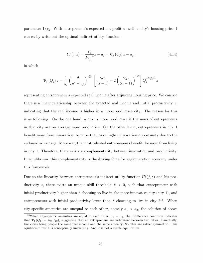
One of the recent developments among American cities is the diverging trend in theirskill compositions and measured innovation (e.g., patents, venture capital). Over the pastthirty years, skilled cities have become more skilled and more productive, and have expe-rienced faster growth in average wages and housing prices. This geographical divergencehas contributed substantially to the rising inequality in America. This paper constructs amulti-city model of spatial skill sorting to explore the causes of this divergence. The keyidea is that cities with advantages in innovation attract more productive entrepreneurs andmore workers, thereby driving up wages and housing prices. I then show that the chang-ing technologies have reinforced the geographical sorting of skills. Specifically, three typesof technological changes have increased the benefits of skill clustering in innovative cities:general productivity increases; improvements in communications technologies; and declinesin trade costs.
∗I am indebted to professor Todd Schoellman, Gustavo Ventura, and Galina Vereshchagina for theirinvaluable guidance and support throughout this project. I also benefited from the comments received fromNatalia Kovrijnykh, Alexander Bick, Domenico Ferraro and other seminar as well as conference participantsin Arizona State University. I would like to give special thanks to my advisor Todd Schoellman, who taughtme a great deal of economic research. Any errors are my own.
†Minjuan Sun: PhD in Department of Economics, Arizona State University. Email: [email protected]
1
1 Introduction
Over the past three decades, the spatial distribution of skills have become increasingly more
dispersed, with the robust feature that the initially skilled cities are becoming more and
more skilled1. The process of differently skilled individuals being sorted into different cities
is called spatial sorting. The direct result of spatial sorting is the phenomenon some refer
to as “the Great Divergence” among American cities. Successful cities have attracted more
and more highly-talented people and enabled them to work collaboratively. Meanwhile,
these cities are experiencing higher population, wage and housing price growth than the
rest of cities. With the fast advancement in technology, people’s capability for long-distance
communication and shipping goods over long distances have vastly improved. Therefore
the need for spatial concentration should have decreased. However, exactly the opposite
is happening in the real world. Behind this increased trend of skill sorting and urban
inequality, lies a puzzling question. Why do people, especially the most talented people,
keep moving towards large cities, without regard to their extremely high living costs?
In modern society, the role of cities in accelerating the flow of technology and ideas has
taken a central place. The geographic density provided by cities brings people together, and
this proximity stimulates idea spread and enables collaboration. Talented people cluster not
simply because they like each other’s company or they prefer urban centers with far superior
amenities, but because they can enjoy productive advantages and knowledge spillovers
that such concentrations bring. As of 2013, about 53% of the top 5% earners in U.S.
metropolitan areas are located in the top 20 large cities. This is an increase from 39% in
19802. Meanwhile, there is unprecedented concentration of innovation activities happening
in these cities. About half of the new product innovations in the 1980s occurred in just1Many papers have studied this phenomenon, such as Goldin and Katz (2007), Ganong and Shoag
(2016), Moretti (2012) and Diamond (2016).2The metropolitan population share in these 20 cities have increased from 22% in 1980 to 29% in 2013.
2
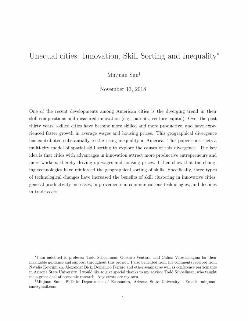
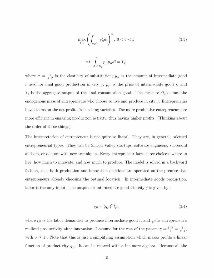
four metropolitan areas: Boston, New York, San Francisco, and Los Angeles3. And almost
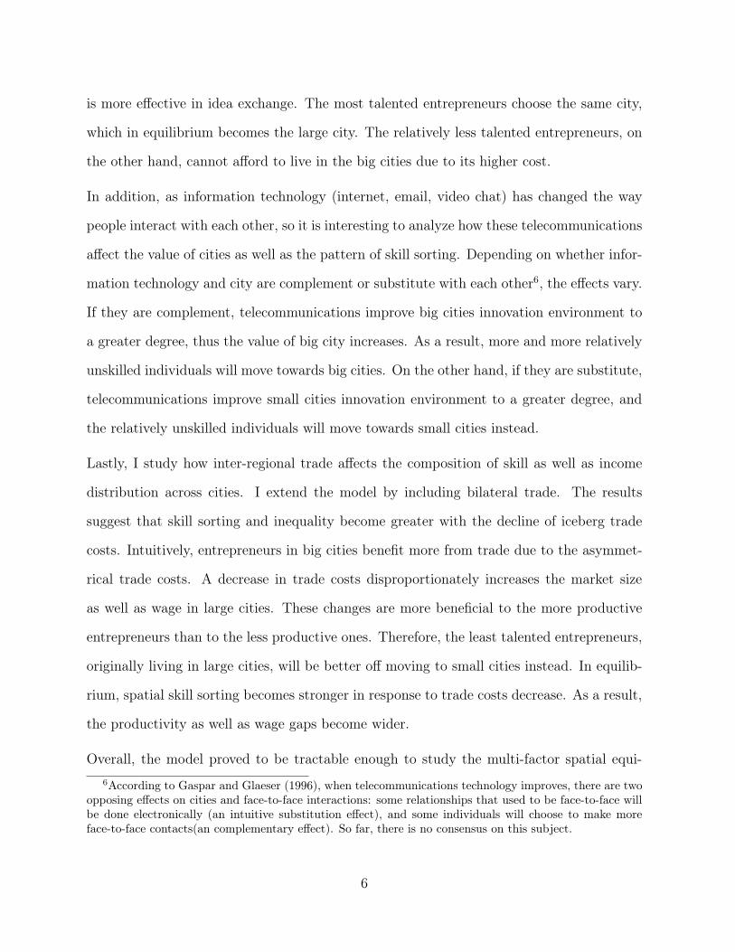
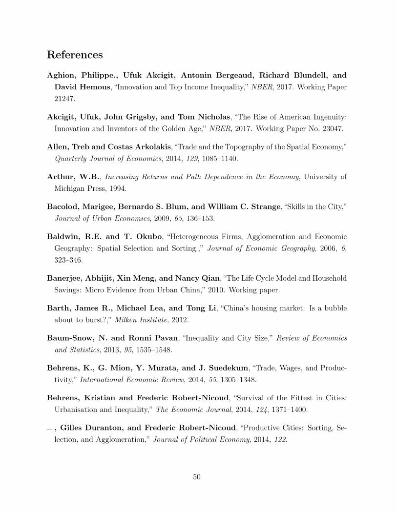
all VC investments were made in major cities, see figure 1.1.
Figure 1.1: Spatial concentration of US patenting and venture capital
Note: VC calculations use the share of deals over the 1990-2005 period. Patent calculations usethe share of granted patents applied for from each city during 1990–2005. The population share isfrom 1999. The figure is taken from Chatterji et al. (2014). Source data are from VentureXpert,USPTO patent data, and county level population statistics.
To explain the increasing trend of spatial skill sorting and innovation concentration, this
paper formulates a multi-city model of innovation and production. The model allows for
two types of agents: production workers and entrepreneurs. Production workers are kept
relatively simple: they simply produce and consume. Entrepreneurs are monopolistic com-
petitors who differ in productivity4. Entrepreneurs run firms and innovate, which increases
their productivity. If an entrepreneur decides to innovate, he pays a cost in return for a ran-
dom productivity draw from the entrepreneurial productivity distribution of the aggregate3This empirical findings about spatial concentration of the commercialization of innovation can be found
in Feldman and Audretsch (1999). For R&D activity, Buzard and Carlino (2013) showed that the spatialconcentration of establishments undertaking R&D is more pronounced than firms.
4The setting of entrepreneurs are similar to that of the standard heterogenous firm model in Merlitz(2003).
3
economy.
Both workers and entrepreneurs choose which of two cities to live and work in. The cities
are identical except that one (generically, the first city) has an endowed advantage in aiding
innovation. I think of this policy as capturing rules, regulations, and the endowment of com-
plementary inputs such as input suppliers, universities, and so on5. This endowed advantage
of the first city is balanced by congestion costs that are in equilibrium stronger, inducing
a non-trivial sorting problem. Every entrepreneur wants to live in the city with better in-
novation environment, since it offers them the best chance to improve their productivities.
But only the more talented ones are able to survive the competition. The complementarity
between agglomeration economies—innovation in this paper—and entrepreneurs’ produc-
tivity leads to the sorting of more skilled entrepreneurs into larger cities. In equilibrium,
they invest more resources on innovation and pay higher wages to workers. In summa-
tion, the interactions between innovation, sorting, and agglomeration economies shape the
income distribution and exacerbate inequality across cities of different sizes.
I start by showing that the model equilibrium allows us to understand the facts outlined
above. The large city attracts more talented entrepreneurs who innovate more, leading
to a higher average productivity. Those more productive entrepreneurs pay higher wages,
which then attract more workers to city 1. This establishes a link between productivity and
city size. On the other hand, the agglomeration forces are inevitably met with congestion
forces: higher housing prices and negative amenity caused by overcrowding. Furthermore,5Traditional discussions of natural advantages focus on geographic features such as harbors and coal
mines. The rise of New York in the early nineteenth century is the result of its central location andprotected harbor which made it the natural hub of shipping and immigration system. But, the technologyadvancement has rendered these geographic features less relevant over time. Bleakley and Lin (2012)believed that the early developed cities have some long-lived assets that could coordinate contemporaryinvestment and cause a persistent effect. Apart from these, factors such as local policies or proximity touniversities and financial institutes can be important as well. For instance, some believe Silicon Valley andBoston became important centers for innovation in part because of their proximity to Stanford Universityand MIT (Lee and Nicholas, 2013). And the lack of “noncompete and nondisclosure clauses” policy doset California apart from other states. The “noncompete and nondisclosure clauses” restrict workers fromstarting new businesses that could possibly in direct competition with their old employers.
4
this model generates two straightforward implications on spatial inequality. First, the
productivity premium of the large city, resulted from skill sorting and intense innovation,
leads to a wage gap across cities. Second, the large city is more unequal comparing to
the small one, because entrepreneurs in large city benefit the most from both the superior
innovation environment and larger market share.
Next, I use the comparative statics of the model to establish some insights on possible
driving forces behind the increased sorting by cities over the last fifty years. In particular,
I show that a simple exogenous rise in total factor productivity (TFP) can induce stronger
skill sorting. Whenever aggregate TFP rises, every city becomes more productive, indicat-
ing that every city’s wage and housing price will rise as well. But the average wage and
housing price in in large city increase more, thus leading to a tough selection. In response,
the marginal entrepreneurs in large city will be better off moving to small city, which then
raises both city’s productivity. But the productivity in big city disproportionately increases
more because of the complementarity between innovation and entrepreneurial productivity.
In this paper, the aggregate TFP is described by the distribution of entrepreneurs’ produc-
tivity. Since productivity follows a Pareto distribution in the model, an increase in TFP can
be proxied by an increase in the minimum productivity threshold, which effectively depicts
the catching up of the least talented entrepreneurs in small cities (Tonetti and Perla, 2014).
Due to the fat tail property of Pareto distribution, the productivity in large city actually
increase more. Therefore, the equilibrium productivity and wage gaps across different sized
cities grow over time.
In the baseline model, the result of perfect skill sorting hinges on the assumption that one
city has exogenous innovation advantage. One way to remedy this is to include localized
knowledge spillover effect. In section 4, I extend the model by assuming that cities have no
fundamental differences, instead the process of innovation is slightly altered. Now knowl-
edge spread is more likely to occur if agents live in the same place, since face-to-face meeting
5
is more effective in idea exchange. The most talented entrepreneurs choose the same city,
which in equilibrium becomes the large city. The relatively less talented entrepreneurs, on
the other hand, cannot afford to live in the big cities due to its higher cost.
In addition, as information technology (internet, email, video chat) has changed the way
people interact with each other, so it is interesting to analyze how these telecommunications
affect the value of cities as well as the pattern of skill sorting. Depending on whether infor-
mation technology and city are complement or substitute with each other6, the effects vary.
If they are complement, telecommunications improve big cities innovation environment to
a greater degree, thus the value of big city increases. As a result, more and more relatively
unskilled individuals will move towards big cities. On the other hand, if they are substitute,
telecommunications improve small cities innovation environment to a greater degree, and
the relatively unskilled individuals will move towards small cities instead.
Lastly, I study how inter-regional trade affects the composition of skill as well as income
distribution across cities. I extend the model by including bilateral trade. The results
suggest that skill sorting and inequality become greater with the decline of iceberg trade
costs. Intuitively, entrepreneurs in big cities benefit more from trade due to the asymmet-
rical trade costs. A decrease in trade costs disproportionately increases the market size
as well as wage in large cities. These changes are more beneficial to the more productive
entrepreneurs than to the less productive ones. Therefore, the least talented entrepreneurs,
originally living in large cities, will be better off moving to small cities instead. In equilib-
rium, spatial skill sorting becomes stronger in response to trade costs decrease. As a result,
the productivity as well as wage gaps become wider.
Overall, the model proved to be tractable enough to study the multi-factor spatial equi-6According to Gaspar and Glaeser (1996), when telecommunications technology improves, there are two
opposing effects on cities and face-to-face interactions: some relationships that used to be face-to-face willbe done electronically (an intuitive substitution effect), and some individuals will choose to make moreface-to-face contacts(an complementary effect). So far, there is no consensus on this subject.
6
librium system. It offers some insights on what caused the geographic divergence among
American cities with respect to productivity, wage and inequality, and what factors con-
tribute to the deeper and growing trend in spatial skill sorting. In addition, I also stress
the role of TFP increase and trade in increasing the relevant market size, which reinforces
skill sorting, sustains larger and more productive cities.
1.1 Related Literature
There are three strands of literature closely related to this paper. The first relevant lit-
erature is about the cross-sectional skill sorting across cities (Behrens and Robert-Nicoud
(2014); Behrens, Duranton and Robert-Nicoud (2014b); Eeckhout, Pinheiro and Schmid-
heiny (2014); Gennaioli, La Porta, Lopez-de Silanes and Shleifer (2013)). Behrens, Du-
ranton and Robert-Nicoud (2014b) developed a multi-city model that explained the com-
plementarities between skill sorting, occupation selection, and agglomeration economies.
They successfully replicated the stylized facts about sorting, agglomeration, and selection
in cities. The main force of agglomeration in their model comes from scale effect: the en-
trepreneurial productivity gain increases with city population size. This approach proves
to be effective in analyzing city’s cross sectional skill sorting and size distribution. Plus
the selection of entrepreneurs within each city provides plenty of productivity overlapping
across cities, which is a nice feature, because in real world skill sorting is imperfect. This
paper is built on their framework, and it has one major difference: the productive advantage
(or innovation advantage) of large cities is allow to be endogenous.
The second relevant literature is focuses on localized knowledge spillover effects on individ-
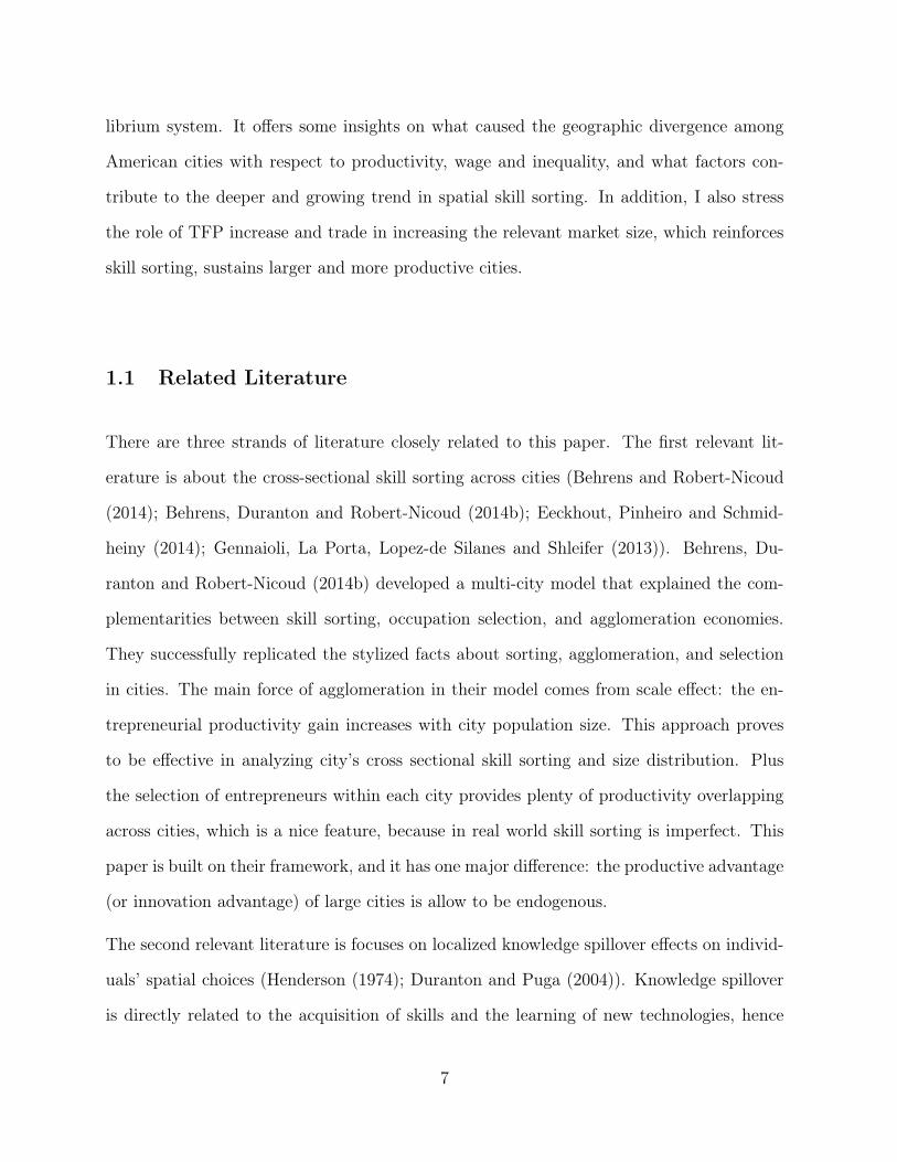
Growth 6.09% 7.79% Growth 0.64% 2.19%(Note: Small city refers to MSAs with less or equal to 1 million population, whereas big city refersto the ones with more than 1 million population.)
2 Motivating Evidence
Empirical evidence that motivating this paper is that big cities have higher productive
advantages for firms, and higher income premium for workers. It is even better if there
are evidence to suggest that the main benefits of living in big cities come from knowledge
spillover effect.
la Roca and Puga (2017) was an important empirical study of the positive relationship
between city size and labor income as well as income growth. They studied Spain’s la-
bor market by cities, and found that workers in big cities not only have higher earnings,
they also have higher growth rates in earnings. The interpretation of income growth is
human capital accumulation through experience. Their result indicates that the experience
accumulated in bigger cities is substantially more valuable than experience accumulated
in smaller cities, and these experience is even more valuable for workers with higher abil-
ity. And it directly prove that there are important learning benefits to working in bigger
cities which is embedded in workers’ human capital. The implication of their analysis is
an important premise for this paper: the advantages of living in big cities come from the
opportunities they provide for individuals to learn from others, and the learning benefit is
greater for people with higher abilities.
There are many ways that make cities different: size, productivity and living cost. But
most fundamentally, cities differ in the composition of human capital. In recent literature,
9
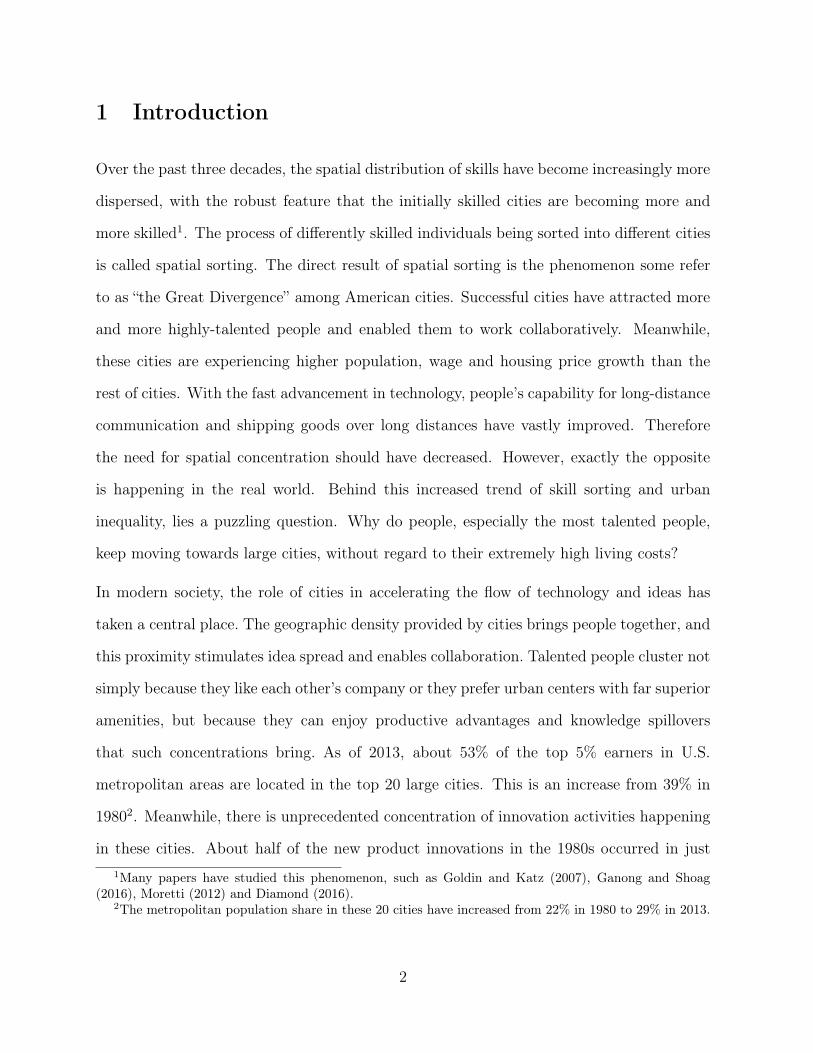
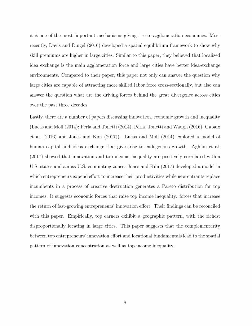
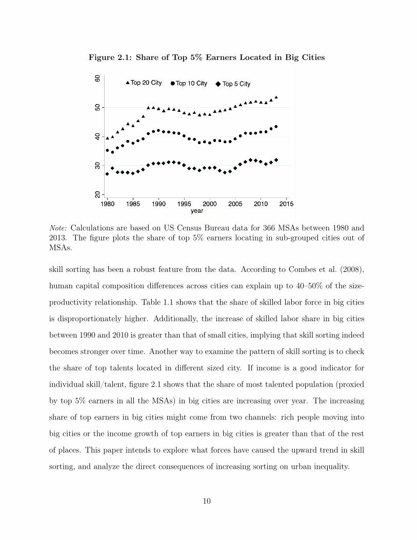
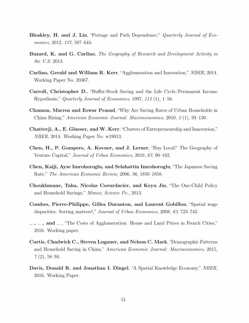
Figure 2.1: Share of Top 5% Earners Located in Big Cities
Note: Calculations are based on US Census Bureau data for 366 MSAs between 1980 and2013. The figure plots the share of top 5% earners locating in sub-grouped cities out ofMSAs.
skill sorting has been a robust feature from the data. According to Combes et al. (2008),
human capital composition differences across cities can explain up to 40–50% of the size-
productivity relationship. Table 1.1 shows that the share of skilled labor force in big cities
is disproportionately higher. Additionally, the increase of skilled labor share in big cities
between 1990 and 2010 is greater than that of small cities, implying that skill sorting indeed
becomes stronger over time. Another way to examine the pattern of skill sorting is to check
the share of top talents located in different sized city. If income is a good indicator for
individual skill/talent, figure 2.1 shows that the share of most talented population (proxied
by top 5% earners in all the MSAs) in big cities are increasing over year. The increasing
share of top earners in big cities might come from two channels: rich people moving into
big cities or the income growth of top earners in big cities is greater than that of the rest
of places. This paper intends to explore what forces have caused the upward trend in skill
sorting, and analyze the direct consequences of increasing sorting on urban inequality.
10
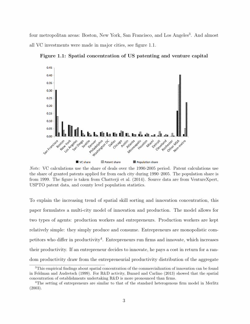
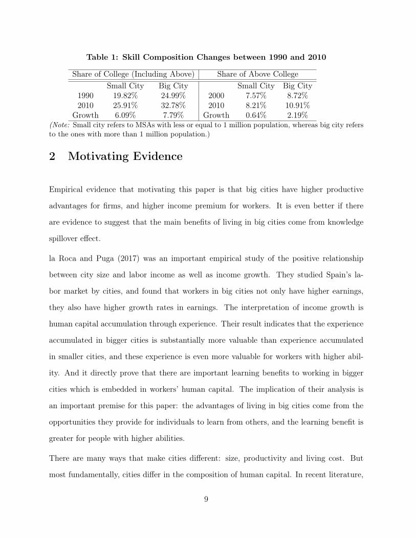
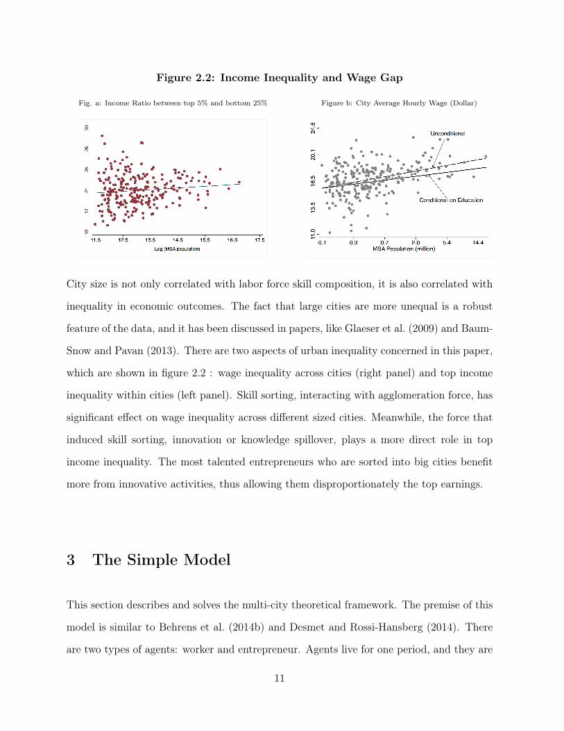
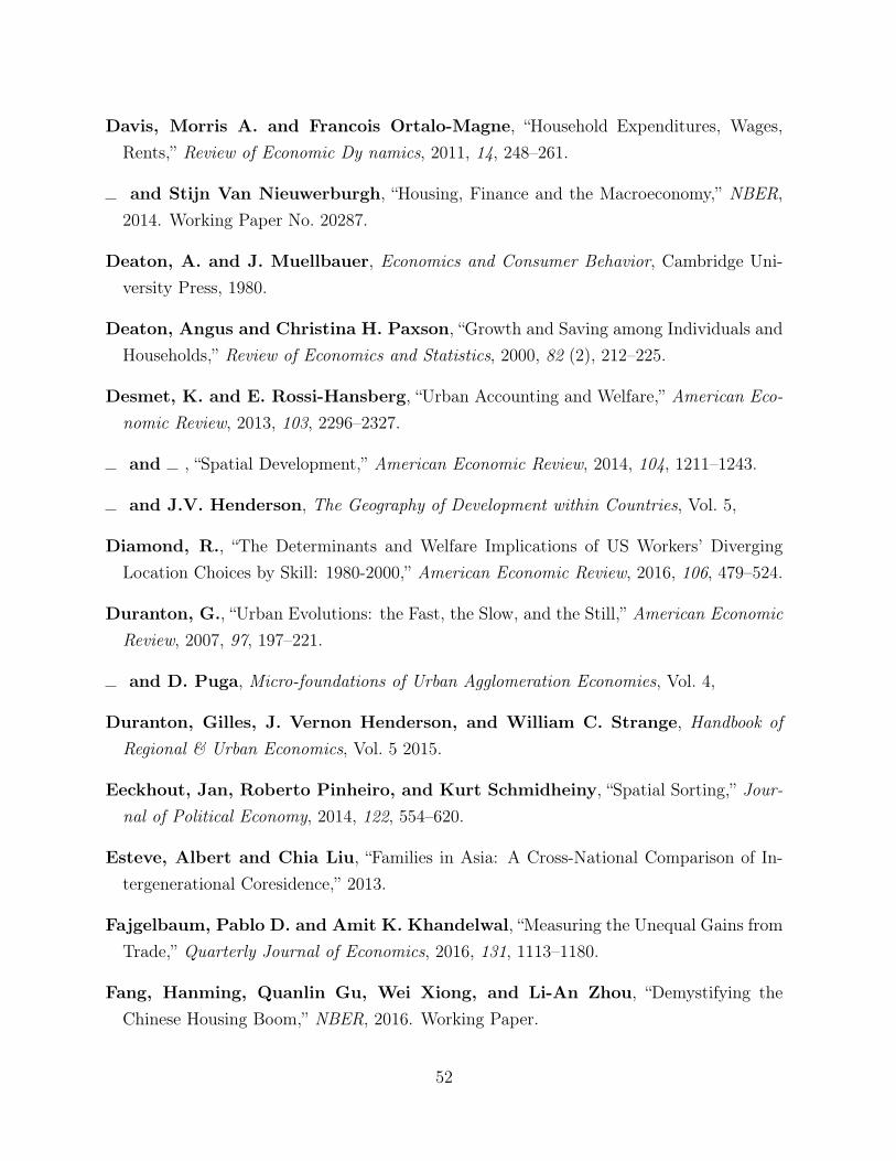
Figure 2.2: Income Inequality and Wage Gap
Fig. a: Income Ratio between top 5% and bottom 25% Figure b: City Average Hourly Wage (Dollar)
City size is not only correlated with labor force skill composition, it is also correlated with
inequality in economic outcomes. The fact that large cities are more unequal is a robust
feature of the data, and it has been discussed in papers, like Glaeser et al. (2009) and Baum-
Snow and Pavan (2013). There are two aspects of urban inequality concerned in this paper,
which are shown in figure 2.2 : wage inequality across cities (right panel) and top income
inequality within cities (left panel). Skill sorting, interacting with agglomeration force, has
significant effect on wage inequality across different sized cities. Meanwhile, the force that
induced skill sorting, innovation or knowledge spillover, plays a more direct role in top
income inequality. The most talented entrepreneurs who are sorted into big cities benefit
more from innovative activities, thus allowing them disproportionately the top earnings.
3 The Simple Model
This section describes and solves the multi-city theoretical framework. The premise of this
model is similar to Behrens et al. (2014b) and Desmet and Rossi-Hansberg (2014). There
are two types of agents: worker and entrepreneur. Agents live for one period, and they are
11
free to move across cities. In particular, they have preferences over good consumption and
housing. I will describe the production and agent decisions in turn.
3.1 City
This paper considers an economy with two cities j 2 {1, 2}. There is a fixed housing
supply, ¯Hj, which is owned by landlords who only consume final consumption goods. Aside
from housing supply, cities are different with respect to only one locational characteristic:
the first city (generically) has an endowed advantage in aiding innovation. The innovation
advantage of city 1 is going to play an important role in what type of agents are going to
be sorted into each city.
3.2 Agent’s Problem
As introduced above, the economy includes two types of agents: workers and entrepreneurs.
There are L identical workers, who consume and produce. And there is a continuum of
entrepreneurs of mass ⌦, who differ in productivity. Each entrepreneur is a monopolist
who produces a differentiated intermediate good. Based on productivity, entrepreneurs
choose where to locate. After moving into a city, they can also innovate, which allows them
to produce their variety more productively.
12
3.2.1 Worker’s Problem
All workers are endowed with one unit of labor, which they supply inelastically. In each city,
workers’ total income is equal to the nominal wage, which is spent on final consumption
good (serving as numeraire) and housing. The utility function for a worker facing wage wj
and housing price Phj in city j is Cobb-Douglas form 7:
UW(j) = max
Cj,Hj
✓Cj
µ
◆µ✓Hj
1� µ
◆1�µ
� aj;
s.t. Cj + PhjHj = wj. (3.1)
where Cj represents final goods consumption, Hj represents housing consumption, and aj is
city-specific congestion amenity. In this paper, congestion amenity refers to the amenities
resulting from overcrowding8, such as long commuting time, pollution, crime, or simply the
difficulty to find a parking space. Because agents are perfectly mobile across cities, and all
workers are ex-ante identical by assumption, then workers will be indifferent between living
in two cities.
7For empirical evidence using U.S. data in support of the constant housing expenditure share impliedby the Cobb-Douglas functional form, see Davis and Ortalo-Magne (2011).
8This model assumes that congestion amenity is fixed, rather than an increasing function of populationsize. If I adopt a different approach, such that aj = L⇢
j , with ⇢ representing the congestion elasticity w.r.tcity population. I can still solve the model, except it is more difficult. The literature on the estimates ofcongestion elasticity ⇢ is quite sparse, so far, I am only aware of Combes et al. (2016). In Duranton et al.(2015), they believed that this congestion elasticity should be very small, which is close to 2%. However,the congestion cost in their definition mostly includes land and housing prices. In this paper, the congestionforce resulted from housing price is included in variable Phj . Therefore, the congestion elasticity in thispaper should be even smaller, which indicates that as city’s population size increases, its congestion amenityincreases but only very barely.
13
3.2.2 Entrepreneur’s Problem
The entrepreneur’s preference is similar to that of worker. The major difference is that
wages. Because innovation is a random process, so entrepreneur’s profit is uncertain. But,
I can still define the expected utility of entrepreneur i, who chooses to live in city j and
has an initial productivity z:
U ei (j, z) = max
Cji,Hji
✓Cji
µ
◆µ✓Hji
1� µ
◆1�µ
� aj; (3.2)
s.t. Cji + PhjHji = ⇧ji (z) .
Where ⇧ji (z) stands for expected net profit, which is the result of endogenous choices on lo-
cation, innovation and production decisions. In the next section, the setup of entrepreneur’s
production and innovation problems are introduced in detail.
3.3 Production
The structure of production within a city is a two-step process: intermediate goods and
final output good. In each city there is a final good producer that supplies the final output
good competitively. The final good is produced by aggregating the mass of intermediate
varieties that are provided by monopolistically competitive entrepreneurs. And it serves
as numeraire in both cities, thus its price is set to 1. The final good producer chooses the
quantity to purchase of each variety:
14
max
yji
ˆi2⌦j
y✓jidi
! 1✓
, 0 < ✓ < 1 (3.3)
s.t.
ˆi2⌦j
pjiyjidi = Yj.
where � =
11�✓ is the elasticity of substitution; yji is the amount of intermediate good
i used for final good production in city j, pji is the price of intermediate good i, and
Yj is the aggregate output of the final consumption good. The measure ⌦j defines the
endogenous mass of entrepreneurs who choose to live and produce in city j. Entrepreneurs
have claims on the net profits from selling varieties. The more productive entrepreneurs are
more efficient in engaging production activity, thus having higher profits. (Thinking about
the order of these things)
The interpretation of entrepreneur is not quite so literal. They are, in general, talented
entrepreneurial types. They can be Silicon Valley startups, software engineers, successful
authors, or doctors with new techniques. Every entrepreneur faces three choices: where to
live, how much to innovate, and how much to produce. The model is solved in a backward
fashion, thus both production and innovation decisions are operated on the premise that
entrepreneurs already choosing the optimal location. In intermediate goods production,
labor is the only input. The output for intermediate good i in city j is given by:
yji = (qji)� lji, (3.4)
where lji is the labor demanded to produce intermediate good i, and qji is entrepreneur’s
realized productivity after innovation. I assume for the rest of the paper: � =
1�✓✓
=
1��1 ,
with � � 1 . Note that this is just a simplifying assumption which makes profits a linear
function of productivity qji. It can be relaxed with a bit more algebra. Because all the
15
labor resource is used to produce intermediate goods, then the labor market constraint is :
L1 + L2 = L; Lj =
ˆi2⌦j
ljidi. (3.5)
It means that out of the aggregate population L, there are L1 workers choosing city 1
and L2 workers choosing city 2 in equilibrium. Next I introduce the process of innovation.
Entrepreneurs need to decide whether and how much to invest in innovation.
3.4 Innovation
Entrepreneurs have differentiated productivity, which can be understood as their skill level
or talent. Each entrepreneur is identified by a draw of productivity z from a Pareto distri-
bution G(·), which is described by its cumulative distribution function (cdf) Pr (z > zmin) =
1 ��zminz
�↵; where zmin is the minimum productivity threshold, and ↵ is the Pareto tail
parameter governing dispersion.
Upon choosing a location, each entrepreneur can improve his productivity through buying
a chance of a new draw from distribution G(·). This innovation process can be understood
as people learning from one another, which is similar to the interpretation in Lucas and
Moll (2014)9. On the other hand, it can also be thought of as tangible or intangible
investments that manifest themselves as improvements in productivity such as improved
production practices, work practices, management practices, etc. see discussions in Holmes
and Schmitz (2010).
Similar to the set-up of Desmet and Rossi-Hansberg (2014), an entrepreneur i with initial9In the baseline model, an entrepreneur in city 1 can improve his productivity by learning from en-
trepreneurs in city 2, without occurring extra innovation cost than he learns from those locating in thesame city. An extended model of localized knowledge spillover is introduced in section 4, in which learningfrom distant cities is more costly than learning within the same city.
16
productivity z in city j can decide to buy a probability �ji 1 of innovating at cost
(�ji | z), which is paid out of the profit from selling variety. This process dictates that
entrepreneur obtains an innovation with probability �ji, and with probability (1� �ji) his
productivity is not affected by the investment in innovation. The entrepreneur who obtains
a chance to innovate draws a new skill z+ from distribution G(z). The new productivity is
adopted if it is higher than the initial productivity, z+ > z; if not, entrepreneur will operate
at his initial productivity level z. Then the expected productivity conditional on the initial
z is:
E�z+ | z, innovation
�=
ˆ 1
zmin
max {x, z} dG(x) =↵z
↵� 1
;
The added “plus” superscript refers to the productivity after the innovation decision. The
expected productivity for entrepreneur i (with initial productivity z) is:
qji (z) = �ji
ˆ 1
z
xdG(x)
| {z }expected productivity if innovate
+ (1� �ji) z| {z }innovation not occur
(3.6)
Finally, I make some assumptions on the primitives of the model. I assume that the
innovation cost function ' (�ji | z) :
@' (�ji | z)@�ji
> 0 and@'2
(�ji | z)@�2
ji
> 0 for �ji 2 (0, 1).
and for any z � zmin:
' (�1i | z) < ' (�2i | z) . (3.7)
These two assumptions make sure that for any given productivity z: (i) the innovation
17
cost is a convex function of innovation opportunity �ji, so that there is no corner solution
problem; (ii) the innovation cost required in city 1 is lower than that in city 2, which is
basically stating that the first city has endowed innovation advantage.
Before the model is solved, I need to formally define the spatial equilibrium. Given initial
productivity distribution G(z), city-specific innovation advantage �j and housing supply ¯Hj , a
spatial equilibrium is a set of real functions {Phj , wj , Cj , Hj , lji, �ji, Yj , Qj , Lj , ⌦j} of city j
and entrepreneur i, such that:
• Given city-specific wage wj and house price Phj , workers choose consumption bundle
{Cj , Hj}, and then locate optimally by solving problem (3.1);
• Ex-ante identical workers are indifferent between two cities, and the indifference con-
dition leads to city’s labor supply Lj, which is expressed in (4.12);
• Entrepreneurs choose optimal location by solving problem (3.2), and the mass of en-
trepreneurs choosing city j is characterized by ⌦j ;
• Given initial productivity z and location choice, each entrepreneur chooses innovation
opportunity �ji by solving problem (4.1);
• Given city’s wage wj, each entrepreneur chooses the number of workers lji to maximize
profit;
• City’s productivity Qj is the average productivity of the mass of entrepreneurs ⌦j
choosing city j, its expression is given in (4.10);
• The model assumes that the aggregate housing value is a constant share (�) of the
aggregate output Yj10. Given housing price Phj, the housing market clearing condition
is ¯HjPhj = �Yj;10The assumptions on land market is similar to Davis and Nieuwerburgh (2014) and Redding and Rossi-
Hansberg (2016b).
18
• Labor market clear, so Lj satisfied condition (3.5).
4 Model Results
Because an entrepreneur’s decisions are rather complicated, I summarize them into four
steps, which then serve as a roadmap for the actual solution process. Since I solve the
model in a backward fashion, the process is as following:
1. Given city’s wage wj, entrepreneurs choose the optimal labor demand lji to maximize
the expected profit E (⇡ji | z) from selling varieties. The detailed steps for solving the
expected profit E (⇡ji | z) is given in appendix A1.
2. Second, given initial productivity z and location j, entrepreneur i chooses innovation
opportunity �ji to maximize the expected net profit ⇧ji (z):
⇧ji (z) = max
�jiE (⇡ji | z)� ' (�ji | z) ; (4.1)
3. Third, with the expected net profit ⇧ji (z), entrepreneur i solves the consumption
maximization problem described in (1.3.2), and get optimized expected utility U ei (j, z).
4. Lastly, to decide the optimal location, he just needs to choose the city with higher
utility:
max
j2{1,2}U ei (j, z). (4.2)
For an entrepreneur with initial productivity z, if U ei (1, z) > U e
i (2, z), he chooses city 1; if
19
U ei (1, z) < U e
i (2, z), he chooses city 2; if U ei (1, z) = U e
i (2, z), he is indifferent between living
in two cities;
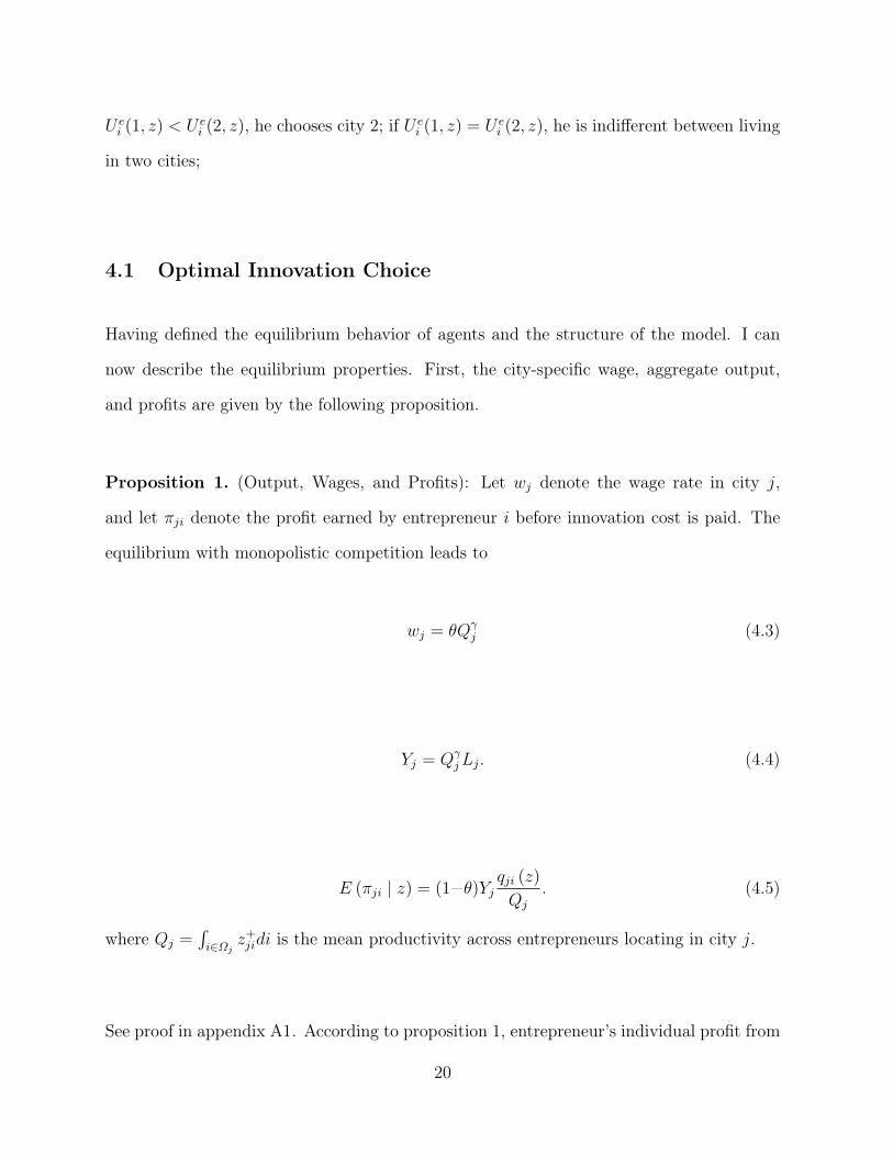
4.1 Optimal Innovation Choice
Having defined the equilibrium behavior of agents and the structure of the model. I can
now describe the equilibrium properties. First, the city-specific wage, aggregate output,
and profits are given by the following proposition.
Proposition 1. (Output, Wages, and Profits): Let wj denote the wage rate in city j,
and let ⇡ji denote the profit earned by entrepreneur i before innovation cost is paid. The
equilibrium with monopolistic competition leads to
wj = ✓Q�j (4.3)
Yj = Q�jLj. (4.4)
E (⇡ji | z) = (1−✓)Yjqji (z)
Qj
. (4.5)
where Qj =´i2⌦j
z+jidi is the mean productivity across entrepreneurs locating in city j.
See proof in appendix A1. According to proposition 1, entrepreneur’s individual profit from
20
selling variety is proportional to local aggregate output, Yj, and relative productivity, qji(z)Qj
.
Here Qj represents city’s average productivity, and its definition is: Qj =´⌦j
qji (z) dz. As
introduced in section 3.4, innovation improves entrepreneur’s productivity, and it happens
with a chance �ji, which is endogenously determined by weighing the benefit and the cost
of innovation. According to function (3.6), the expected productivity after innovation is:
qji (z) = �ji↵z
↵� 1
+ (1� �ji) z (4.6)
=
✓�ji + ↵� 1
↵� 1
◆
| {z }scale of innovation
z.
The above expression indicates that the benefit of innovation comes from the elevation
of initial productivity z. And the scale of elevation, �ji+↵�1↵�1 , solely depends on innovation
opportunity �ji and Pareto tail parameter ↵. Now, it is time to solve entrepreneur’s optimal
innovation opportunity. To do that, I need to give the specific functional form for innovation
innovation environment. To be consistent with the assumption that city 1 has a better
innovation environment compared to city 2, I let �1 < �211. Note that the innovation
cost function is also increasing in city-specific wage (wj), population size (Li) and relative
productivity zQj
. The increasing relationship between innovation cost and aggregate labor
income wjLj is to capture the labor cost in innovation12. Meanwhile, the more productive11The rationale for one of the city having better innovation environment can be found in footnote 6.12In equilibrium, the aggregate labor income wjLj is proportional to the aggregate output, i.e. Yj =
wjLj
✓ . Then the defined innovation cost function indicates that innovation investment is proportional to
21
entrepreneurs are closer to technology frontier, thus have little room to improve, which is
why their innovation cost is higher.
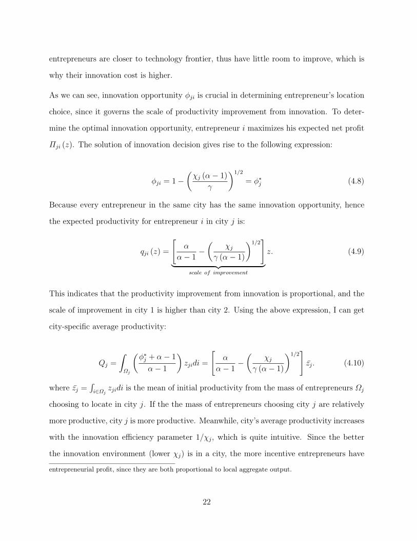
As we can see, innovation opportunity �ji is crucial in determining entrepreneur’s location
choice, since it governs the scale of productivity improvement from innovation. To deter-
mine the optimal innovation opportunity, entrepreneur i maximizes his expected net profit
⇧ji (z). The solution of innovation decision gives rise to the following expression:
�ji = 1�✓�j (↵� 1)
�
◆1/2
= �⇤j (4.8)
Because every entrepreneur in the same city has the same innovation opportunity, hence
the expected productivity for entrepreneur i in city j is:
qji (z) =
"↵
↵� 1
�✓
�j
� (↵� 1)
◆1/2#
| {z }scale of improvement
z. (4.9)
This indicates that the productivity improvement from innovation is proportional, and the
scale of improvement in city 1 is higher than city 2. Using the above expression, I can get
city-specific average productivity:
Qj =
ˆ⌦j
✓�⇤j + ↵� 1
↵� 1
◆zjidi =
"↵
↵� 1
�✓
�j
� (↵� 1)
◆1/2#zj. (4.10)
where zj =´i2⌦j
zjidi is the mean of initial productivity from the mass of entrepreneurs ⌦j
choosing to locate in city j. If the the mass of entrepreneurs choosing city j are relatively
more productive, city j is more productive. Meanwhile, city’s average productivity increases
with the innovation efficiency parameter 1/�j, which is quite intuitive. Since the better
the innovation environment (lower �j) is in a city, the more incentive entrepreneurs have
entrepreneurial profit, since they are both proportional to local aggregate output.
22
to invest in innovation, as a result the scale of productivity improvement will be larger.
4.2 Equilibrium Spatial Sorting
This model involves two types of agents: worker and entrepreneur. Naturally, spatial sorting
refers to the process both types deciding their optimal locations. I will start with worker’s
location choice first, since it is fairly easy.
4.2.1 The Sorting of Workers
Given city-specific housing price and wage, worker solves utility maximization problem
defined in problem (3.1). With constant expenditure shares on final good and housing,
worker’s indirect utility function becomes:
UW(j) =
wj
P 1�µhj
� aj.
The first part of the indirect utility function wj
p1�µhj
represents the real income after adjusting
housing cost, the second part aj represents the congestion amenity. Clearly, worker’s loca-
tion choice is determined by city’s nominal wage and living cost, which includes housing
price and local amenity. This simple utility form is able to accommodate a number of re-
gional differences. The two cities differ in their relative productivity, with more productive
city having higher nominal wage and higher housing price. In equilibrium, ex-ante identical
workers are indifferent between living in two cities. Hence, worker’s indirect utility function
UW(j) equalizes:
w1
p1�µ1j
� a1 =w2
p1�µh2
� a2 = u⇤, (4.11)
23
where u⇤ is the equilibrium common utility level. This indifference condition clearly states
the tradeoff for choosing between two cities: the higher nominal wage in large city must
be balanced out by a higher living cost. Using the housing market clearance condition
¯HjPhj = �Yj, house price can be expressed as a function of wage wj and local population
Lj:
Phj =�Yj
¯Hj
=
�wjLj
✓ ¯Hj
.
Let ⌘j = �✓Hj
, then parameter 1/⌘j can be perceived as land supply coefficient: city’s fixed
housing supply ¯Hj is more restricted when ⌘j is higher. Replacing Phj with ⌘jwjLj in the
indifference equation (4.11), the equilibrium labor supply in city j is
Lj =w
µ1�µ
j
⌘j(u⇤+ aj)
11�µ
. (4.12)
Equation (4.12) represents the labor supply in city j, which is increasing in city’s wage rate,
decreasing in land supply coefficient ⌘j and congestion amenity aj.
4.2.2 The Sorting of Entrepreneurs
An entrepreneur’s sorting problem is similar to that of the worker’s. Each entrepreneur
decides where to live based on three factors: expected entrepreneurial income, housing price
and city-specific congestion amenity. With the optimal innovation opportunity expressed
in (4.8), the equilibrium expected net profit is:
⇧ji (z) = E (⇡ji | z)� '��⇤j | z
�= �jz, (4.13)
where �j = (1 � ✓)
↵
(↵�1) � 2
⇣�j
�(↵�1)
⌘1/2�Yj
Qjsummarizes the benefit of an entrepreneur
choosing city j, which is increasing in city’s aggregate output Yj and innovation efficiency
24
parameter 1/�j. With entrepreneur’s expected net profit as well as city’s housing price, I
can easily write out the optimal indirect utility function:
U ei (j, z) =
�j
P 1�µhj
z � aj = j (Qj) z � aj; (4.14)
in which
j (Qj) z =
1
⌘j
✓✓
u⇤+ aj
◆ µ1�µ
"�↵
(↵� 1)
� 2
✓��j
(↵� 1)
◆1/2#Q
�µ+µ�11�µ
j z
representing entrepreneur’s expected real income after adjusting housing price. We can see
there is a linear relationship between the expected real income and initial productivity z,
indicating that the real income is higher in a more productive city. The reason for this
is as following. On the one hand, a city is more productive if the mass of entrepreneurs
in that city are on average more productive. On the other hand, entrepreneurs in city 1
benefit more from innovation, because they have higher innovation opportunity due to the
endowed advantage. Moreover, the most talented entrepreneurs benefit the most from living
in city 1. Therefore, there exists a complementarity between innovation and productivity.
In equilibrium, this complementarity is the driving force for agglomeration economy under
this framework.
Due to the linearity between entrepreneur’s indirect utility function U ei (j, z) and his pro-
ductivity z, there exists an unique skill threshold z > 0, such that entrepreneur with
initial productivity higher than z choosing to live in the more innovative city (city 1), and
entrepreneurs with initial productivity lower than z choosing to live in city 213. When
city-specific amenities are unequal to each other, namely a1 > a2, the solution of above13When city-specific amenities are equal to each other, a1 = a2, the indifference condition indicates
that 1 (Q1) = 2 (Q2), suggesting that all entrepreneur are indifferent between two cities. Essentially,two cities bring people the same real income and the same amenity. So cites are rather symmetric. Thisequilibrium result is conceptually unexciting. And it is not a stable equilibrium.
25
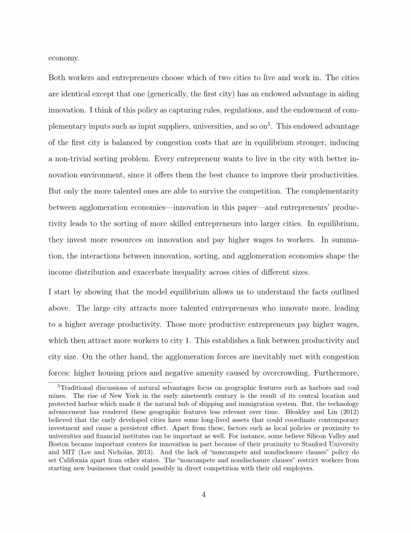
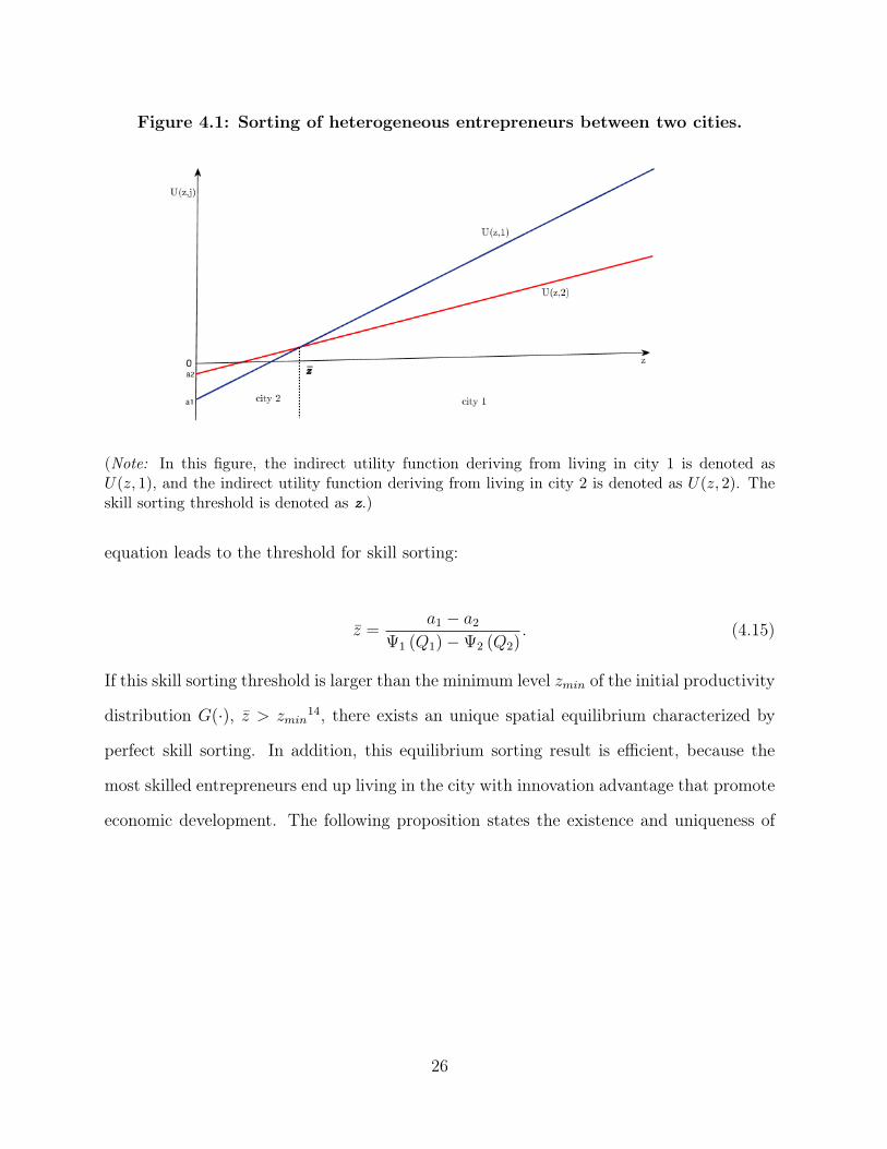
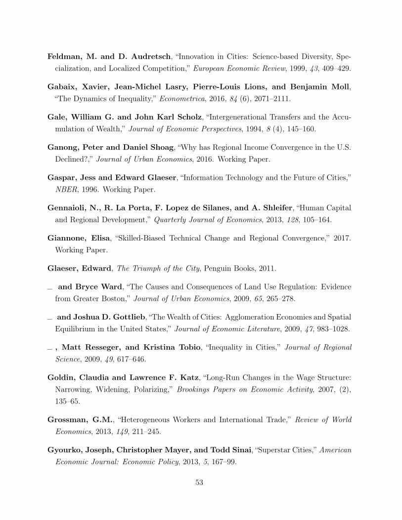
Figure 4.1: Sorting of heterogeneous entrepreneurs between two cities.
(Note: In this figure, the indirect utility function deriving from living in city 1 is denoted asU(z, 1), and the indirect utility function deriving from living in city 2 is denoted as U(z, 2). Theskill sorting threshold is denoted as z.)
equation leads to the threshold for skill sorting:
z =
a1 � a2 1 (Q1)� 2 (Q2)
. (4.15)
If this skill sorting threshold is larger than the minimum level zmin of the initial productivity
distribution G(·), z > zmin14, there exists an unique spatial equilibrium characterized by
perfect skill sorting. In addition, this equilibrium sorting result is efficient, because the
most skilled entrepreneurs end up living in the city with innovation advantage that promote
economic development. The following proposition states the existence and uniqueness of
26
the spatial equilibrium. See proof in appendix A2.
Proposition 2. (Equilibrium Existence and Uniqueness): Assume a1 > a2, �1 < �2 and
�µ+µ� 1 > 0. There exists an unique equilibrium with perfect skill sorting: entrepreneur
with initial skill higher than z choose large city, and entrepreneur with initial skill lower
than z choose small city.
Figure 4.1 illustrates the skill allocation between two cities. From proposition 2, a few
results immediately follow. First, the city with innovation advantage (city 1) has higher
average productivity, since all the most productive entrepreneurs gather in that city. And
their productivity improvement from innovation is higher due to the exogenous innovation
advantage. Second, city 1 has higher nominal wage compare to city 2, because city-specific
wage is positively related to city’s average productivity. Third, the city with innovation
advantage effectively becomes the larger (or denser) city, because workers want to live
in a city with higher wage. Last, the larger city has higher housing price, because both
higher wage and higher population density tend to escalate housing price. These results
are summarized in the following proposition.
Proposition 3. (Equilibrium City Characteristics): Assume city 1 is endowed with inno-
vation advantage: �1 < �2. In equilibrium, city 1 has higher population density, L1
H1> L2
H2,
higher average productivity, Q1 > Q2, higher wage, w1 > w2, and higher housing price,
Ph1 > Ph2.
14Condition z > zmin stipulates that the difference in city-specific amenity, i.e. a1 � a2, should notbe infinitesimally small under the perfect skill sorting equilibrium. Because in the case of a1 � a2 beinginfinitely close to 0, the equilibrium is essentially the symmetrical city structure result that I introducedbefore.
27
As shown in proposition 3, this spatial sorting model can generate results that are com-
patible with city’s cross-sectional stylized facts, such that large cities are more skilled, and
have higher average wages as well as housing prices.
With perfect skill sorting, I can now write down the expressions of average city productiv-
ities:
Q1 =↵
↵�1
↵
↵�1 �⇣
�1
�(↵�1)
⌘1/2�z;
Q2 =↵
↵�1
↵
↵�1 �⇣
�2
�(↵�1)
⌘1/2�zmin
1�(
zminz )
↵�1
1�(
zminz )
↵ .(4.16)
From equation (4.16), we know the relative productivity is increasing in the skill sorting
threshold z:@⇣
Q1
Q2(z)⌘
@z> 0.
It means that the productivity gap across cities is directly linked with skill sorting threshold15. If skill sorting becomes stronger over time, meaning that z " over time, the diverging
trend in productivity and wage gaps across cities can be at least partially explained.
4.3 Top Income Inequality within Cities
So far I have calculated an entrepreneur’s expected income, see equation (4.13). And we
know that workers total income is wjLj, then top income inequality within a city can be
expressed through the ratio between aggregate entrepreneurial income and labor income:
entrepreneur�sharej =
´i2⌦j
⇧ji (z) dz
wjLj
=
"�↵
(↵� 1)
� 2
✓��j
(↵� 1)
◆1/2#
zjQj
,
15Note, the result of@⇣
Q1Q2
(z)⌘
@z > 0 might arise due to the fat tail property of Pareto distribution. It maynot stands if the productivity distribution is symmetrical.
28
where zj is the mean initial skill of the mass of entrepreneurs choosing city j, with zj =
´i2⌦j
zjidi. Taking advantage of expression (4.10), the entrepreneurial income share can be
simplified as:
) entrepreneur�sharej = �
↵(↵�1) � 2
⇣�j
�(↵�1)
⌘1/2
↵(↵�1) �
⇣�j
�(↵�1)
⌘1/2 (4.17)
This expression suggests that a lower �j will raise the entrepreneurial income share, which
relates the innovation activity to income distribution. Formally, this result is shown as:
Proposition 4. (Top Income Inequality within Cities): The share of entrepreneurial in-
come within a city increases with innovation efficiency ( 1�j
). Therefore, assumption �1 < �2
implies that big city is more unequal compared to small city.
According to this proposition, two results stand out. The first is that large city is more un-
equal. This result comes from the complementarity between innovation and entrepreneurial
productivity. Entrepreneurs in the large city benefit more from innovation activity, because
they have higher opportunities to innovate due to the city’s endowed advantage. Therefore,
their income share is higher even though the wage in large city is also higher.
Observing equation (4.17), we can see that the entrepreneurial income share in each city
is completely determined by exogenous parameters: �, ↵ and �j. It suggests that top
income inequality does not change over time, unless the locational innovation advantage
(�j) changes16.
16One way to generate increasing top income inequality is letting model adopt a different innovationcost function which generates additional scale effect. For instance, if the innovation cost in city j is
29
5 Factors Of Increasing Skill Sorting
So far, the model has successfully delivered the right kind of sorting across cities. Now I’m
going to use the comparative statics of the model to try to analyze what kind of forces might
increase sorting and inequality between cities. There are two clear candidates presenting
themselves in this model: TFP growth and locational fundamentals.
The aggregate TFP in this model is essentially the mean of overall entrepreneurial produc-
tivities:
TFP =
ˆ z
zmin
✓�⇤2 + ↵� 1
↵� 1
◆zdG (z)+
ˆ 1
z
✓�⇤1 + ↵� 1
↵� 1
◆zdG (z) = G (z)Q1+(1�G (z))Q2.
Since productivity follows a Pareto distribution, an increase in TFP can be proxied by an
increase in the minimum productivity threshold, zmin, of distribution G(·). With perfect
skill sorting, small city’s average productivity Q2 is increasing in zmin. But large city’s
average productivity Q1 is unaffected by zmin, except through equilibrium sorting threshold
z, see equation (4.16). As proved in appendix A3, the equilibrium sorting threshold z
increases if there is an increase in zmin. It implies that TFP increase will undoubtedly
reinforce the skill sorting process, and increase the productivity gap across cities. This
result is summarized as following:
Proposition 5. (Comparative Statics One): The big city disproportionately benefits from
an increase in the equilibrium skill sorting threshold z. Therefore, the relative productivity
' (�ji | z) = �jwj
1��ji
zQj
, then the equilibrium entrepreneurial income share becomes:
) entrepreneur�sharej = �
↵(↵�1) � 2
⇣�j
�(↵�1)Lj
⌘1/2
↵(↵�1) �
⇣�j
�(↵�1)Lj
⌘1/2 .
The above equation clearly indicates that top income inequality is increasing in city population size Lj .Therefore, any potential forces that make the large city even large will also make it more unequal.
30
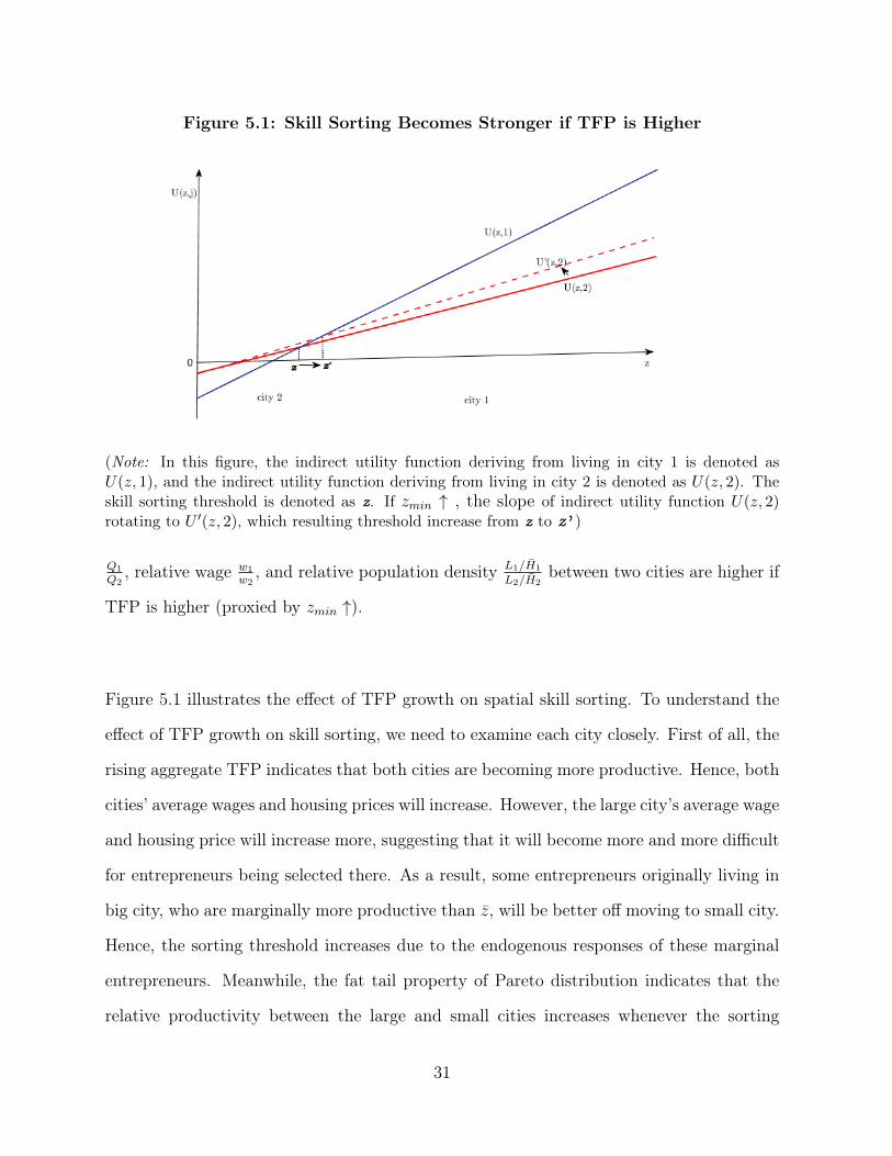
Figure 5.1: Skill Sorting Becomes Stronger if TFP is Higher
(Note: In this figure, the indirect utility function deriving from living in city 1 is denoted asU(z, 1), and the indirect utility function deriving from living in city 2 is denoted as U(z, 2). Theskill sorting threshold is denoted as z. If zmin " , the slope of indirect utility function U(z, 2)rotating to U 0
(z, 2), which resulting threshold increase from z to z’)
Q1
Q2, relative wage w1
w2, and relative population density L1/H1
L2/H2between two cities are higher if
TFP is higher (proxied by zmin ").
Figure 5.1 illustrates the effect of TFP growth on spatial skill sorting. To understand the
effect of TFP growth on skill sorting, we need to examine each city closely. First of all, the
rising aggregate TFP indicates that both cities are becoming more productive. Hence, both
cities’ average wages and housing prices will increase. However, the large city’s average wage
and housing price will increase more, suggesting that it will become more and more difficult
for entrepreneurs being selected there. As a result, some entrepreneurs originally living in
big city, who are marginally more productive than z, will be better off moving to small city.
Hence, the sorting threshold increases due to the endogenous responses of these marginal
entrepreneurs. Meanwhile, the fat tail property of Pareto distribution indicates that the
relative productivity between the large and small cities increases whenever the sorting
31
threshold increases. In that sense, TFP growth is equivalent to small city’s technology
catching up to the big city, and it strengthens the sorting process and raises the productivity
gap in the end.
As for locational fundamentals, there are three factors that can affect the equilibrium
sorting result: innovation advantage (1/�j), land supply (1/⌘j) and congestion amenity
(aj). First of all, the city endowed with innovation advantage in equilibrium becomes the
large city, and it generates higher innovation opportunity, thus entrepreneurs benefit more
from living in that city. Next, a city with more restricted land supply ( higher ⌘j) has higher
equilibrium housing price, which makes the less productive entrepreneurs more deterred.
Third, congestion amenity (aj) represents the downside of living in a over-crowed city, and
people may not want to live in big cities if congestion amenity becomes too high to bear.
The result of comparative statics are shown in proposition 5, and its proof can be found in
appendix A3.
Proposition 6. (Comparative Statics Two): The big city disproportionately benefits from
an increase in the equilibrium skill sorting threshold z. Therefore, the relative productivityQ1
Q2, relative wage w1
w2, and relative population density L1/H1
L2/H2between two cities are: (i)
decreasing in big city’s innovation advantage, 1/�1; (ii) decreasing in big city’s land supply,
1/⌘1. In addition, both relative productivity Q1
Q2and relative wage w1
w2are increasing in
congestion amenity, a1, but the response of relative population density L1/H1
L2/H2to an increase
in a1 is uncertain.
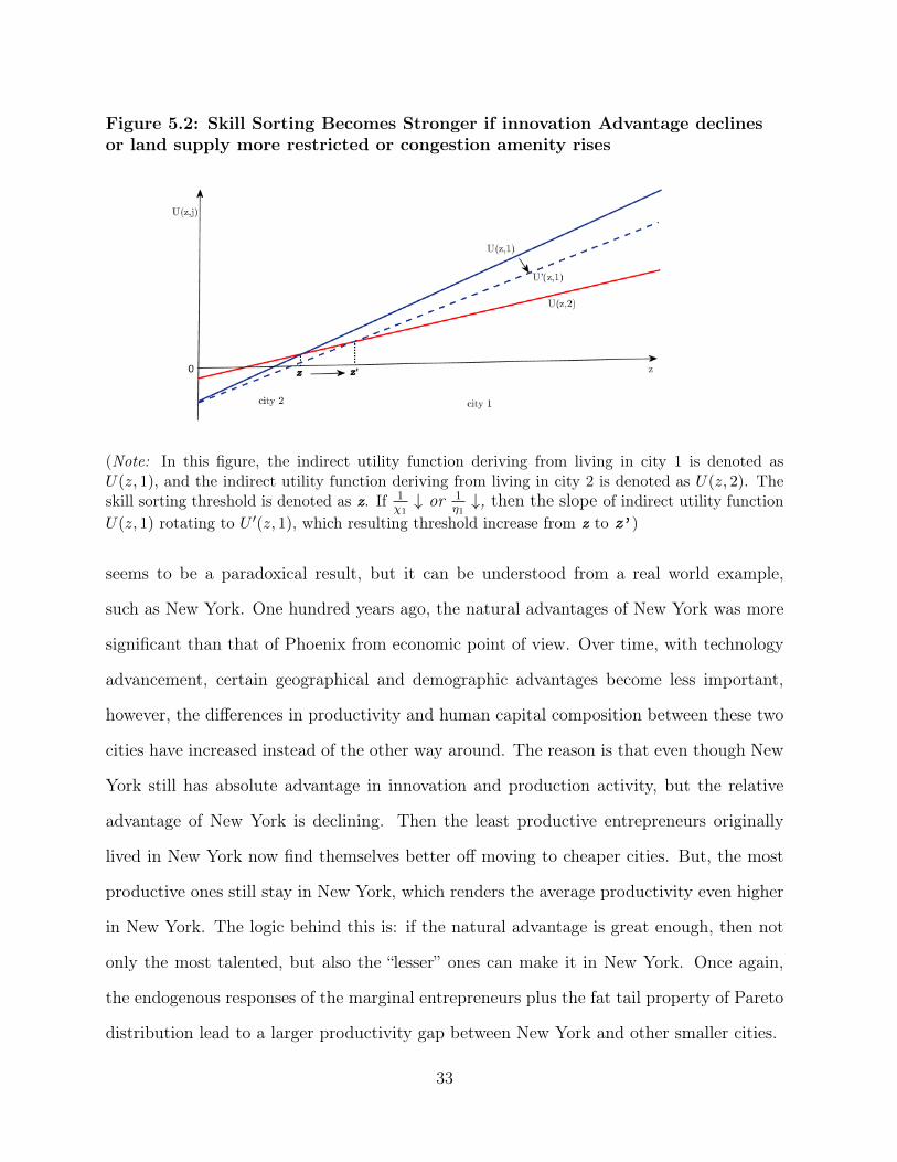
Figure 5.2 illustrates the comparative statics related to spatial skill sorting. There are two
implications from the above proposition. First, if the innovation advantage in large city
is declining relative to that of the small city, then skill sorting becomes stronger. This
32
Figure 5.2: Skill Sorting Becomes Stronger if innovation Advantage declinesor land supply more restricted or congestion amenity rises
(Note: In this figure, the indirect utility function deriving from living in city 1 is denoted asU(z, 1), and the indirect utility function deriving from living in city 2 is denoted as U(z, 2). Theskill sorting threshold is denoted as z. If 1
�1# or 1
⌘1#, then the slope of indirect utility function
U(z, 1) rotating to U 0(z, 1), which resulting threshold increase from z to z’)
seems to be a paradoxical result, but it can be understood from a real world example,
such as New York. One hundred years ago, the natural advantages of New York was more
significant than that of Phoenix from economic point of view. Over time, with technology
advancement, certain geographical and demographic advantages become less important,
however, the differences in productivity and human capital composition between these two
cities have increased instead of the other way around. The reason is that even though New
York still has absolute advantage in innovation and production activity, but the relative
advantage of New York is declining. Then the least productive entrepreneurs originally
lived in New York now find themselves better off moving to cheaper cities. But, the most
productive ones still stay in New York, which renders the average productivity even higher
in New York. The logic behind this is: if the natural advantage is great enough, then not
only the most talented, but also the “lesser” ones can make it in New York. Once again,
the endogenous responses of the marginal entrepreneurs plus the fat tail property of Pareto
distribution lead to a larger productivity gap between New York and other smaller cities.
33
The second implication worth emphasizing is that spatial skill sorting becomes stronger
if big city’s land supply becomes more restricted. This is very intuitive, because only
the richest and the most talented people can afford high housing price. Again, we can
understand it from a real world example. As the innovation cluster center in twenty-first
century, Silicon valley is currently among the most expensive city in United States. However,
the city’s high housing prices reflect more than just good weather and high incomes. The
city has rather severe restrictions on home construction. Between 2001 and 2008, despite
the booming demand, the area’s stock of single-family homes increased by less than 5%,
which was less than 1/3 of the U.S. average building rate over that period. According to
Glaeser (2011), Silicon valley’s housing price would be 40% lower if there is no restriction
on house/land supply.
6 Localized Knowledge Spillover
So far, the baseline model assumes that one city has exogenous innovation advantage, which
attracts the most talented entrepreneurs living there. And these entrepreneurs in turn push
up this city’s wage and housing price, making it too expensive for the relatively less talented
entrepreneurs. As introduced in the abstract, one of the main contributions of this paper
is to build a model that allowing for endogenous innovation advantage. This section is to
formalize that extension through the effect of localized knowledge spillover. According to
Lucas and Moll (2014), entrepreneurs can interact with and learn from other entrepreneurs
in the same place. On top of their idea, I add the spatial aspect which allowing geography
to play a role in the process of idea exchange or innovation. Essentially, innovation is more
likely to happen if entrepreneurs live in the same city with other top talented entrepreneurs,
since face-to-face meeting is the more effective form of human interaction. This extension
34
has the following three merits: (i) it shows that big cities can be endogenously more innova-
tion and more productive without assuming any exogenous fundamental differences across
different cities; (ii) it also allows me to formally analyze how information technology affects
the skill compositions at different cities; (iii) its modeling approach is very similar to that
of the baseline model, hence it preserves the results of the comparative statics from the
baseline model.
To present the idea at its simplest, the innovation technology is similar to that of the
baseline model, except now innovation depends on an endogenous variable: local learning
opportunities (�j). The innovation process is as following. An entrepreneur i in city j can
buy a chance of innovation with probability �ji, however only with chance �j, innovation in
city j can actually occur. With probability (1��ji�j) his productivity remains unchanged,
and the ones obtaining a chance to innovate draws a new skill z+ from distribution G(·).
The expected productivity level conditional on innovation is the same as baseline model:
E�z+ | z, innovation
�=
ˆ 1
z
xdG(x) =↵z
↵� 1
;
the added “plus” superscript refers to the productivity after the innovation decision. The
expected productivity for innovation probability �ji is:
qji (z) = �ji�j↵z
↵� 1| {z }expected productivity if innovate
+ (1� �ji�j) z| {z }innovation not occur
=) qji (z) =⇣�ji�j+↵�1
↵�1
⌘z.
(6.1)
The variable �j stands for local chance of meeting people with higher productivity. For-
mally, local learning environment is characterized by a function �j = �(zj), and �(zj) =
{zj 2 (0,1) : �(zj) 2 (0, 1)}, where zj =
´i2⌦j
zjidi representing the average initial pro-
ductivity of entrepreneurs living in city j. To introduce the learning technology in detail,
35
the following assumption is necessary:
Assumption: �(·) is continuous, concave, and increasing in the average initial productivity
of entrepreneurs, zj, who endogenously choose city j. Meanwhile it has following properties:
�(0) = 0 and �(1) = 1.
The above assumption indicates that as a city becomes more skilled, the chance of its
residents improving productivity is increasing as well. In addition, �(zj) increases faster
as zj is smaller, eventually it slowly approaches 1 when zj approaches infinity. There are
many functions satisfy the above assumption, for analysis purpose, I choose the following
form:
�(zj) =zj
zj + c, c > 0; (6.2)
The production process in this section is the same as the baseline model, indicating that
all the results stated in proposition 1 in baseline model are also valid here. Therefore, the
expected profit from selling variety remains the same: ˜E (⇡ji | z) = �wjLj
Qjqji (z). However,
the baseline model assumes different innovation costs at different locations. The extended
model is designed to eliminate that exogeneity, since it might be mixed with the endogenous
effect of localized idea exchange. Therefore, I assume there is no fundamental differences
in city’s innovation costs:
' (�ji | z) =�z
1� �ji
wjLj
Qj
, � > 0; (6.3)
The process of solving for the optimal innovation opportunity is similar to the baseline
model. Its expression is:
˜�ji = 1�✓� (↵� 1)
��j
◆1/2
=
˜�j (6.4)
Clearly, if a city provides a better chance to meet more productive people, namely a higher
�j, then the equilibrium innovation opportunity ˜�j will be higher, which leads to higher
36
return of innovation investment. Substituting ˜�ji in (6.1) with above equation, we can get
city’s average productivity:
Qj =
ˆ⌦j
˜�j�(zj) + ↵� 1
↵� 1
!zjidi =
"↵� 1 + �(zj)
↵� 1
�✓
��(zj)
� (↵� 1)
◆1/2#
| {z }Scale of improvement due to innovation
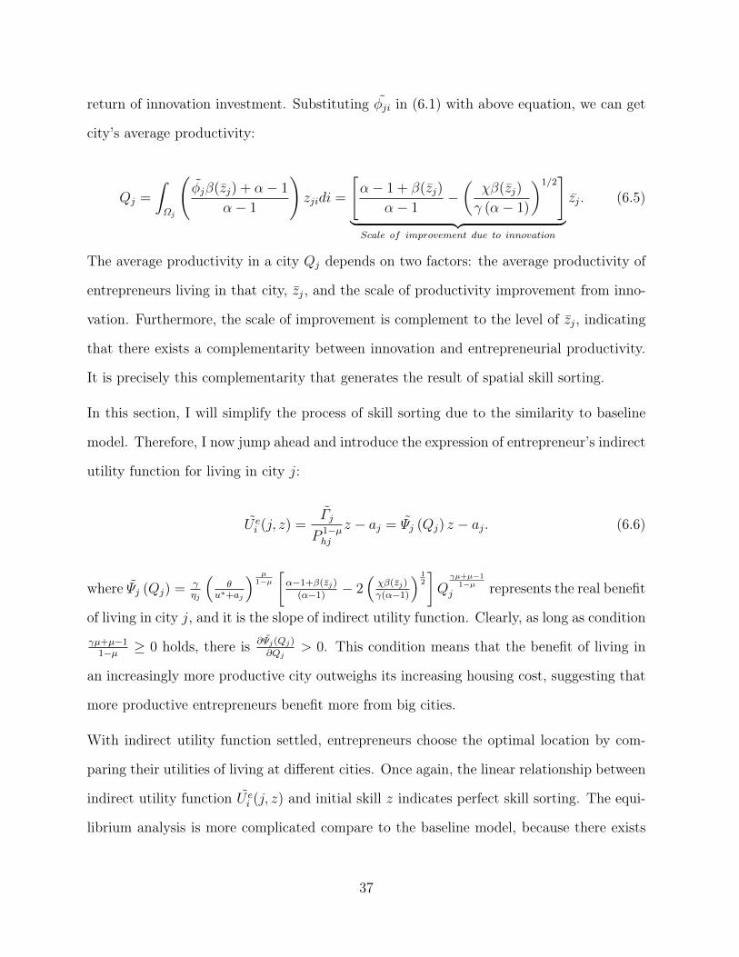
zj. (6.5)
The average productivity in a city Qj depends on two factors: the average productivity of
entrepreneurs living in that city, zj, and the scale of productivity improvement from inno-
vation. Furthermore, the scale of improvement is complement to the level of zj, indicating
that there exists a complementarity between innovation and entrepreneurial productivity.
It is precisely this complementarity that generates the result of spatial skill sorting.
In this section, I will simplify the process of skill sorting due to the similarity to baseline
model. Therefore, I now jump ahead and introduce the expression of entrepreneur’s indirect
utility function for living in city j:
˜U ei (j, z) =
˜�j
P 1�µhj
z � aj = ˜ j (Qj) z � aj. (6.6)
where ˜ j (Qj) =�⌘j
⇣✓
u⇤+aj
⌘ µ1�µ
↵�1+�(zj)
(↵�1) � 2
⇣��(zj)�(↵�1)
⌘ 12
�Q
�µ+µ�11�µ
j represents the real benefit
of living in city j, and it is the slope of indirect utility function. Clearly, as long as condition�µ+µ�1
1�µ� 0 holds, there is @ j(Qj)
@Qj> 0. This condition means that the benefit of living in
an increasingly more productive city outweighs its increasing housing cost, suggesting that
more productive entrepreneurs benefit more from big cities.
With indirect utility function settled, entrepreneurs choose the optimal location by com-
paring their utilities of living at different cities. Once again, the linear relationship between
indirect utility function ˜U ei (j, z) and initial skill z indicates perfect skill sorting. The equi-
librium analysis is more complicated compare to the baseline model, because there exists
37
the possibility of multiple equilibria due to the fact that entrepreneur’s location choice now
depending on other’s choices as well. The first possible equilibrium is that all entrepreneurs
with productivity higher than certain threshold z⇤ choosing city 1, and the second possi-
ble equilibrium is that all entrepreneurs with productivity higher than certain threshold
z⇤ choosing city 2. Since city is generic and has no fundamental differences except for
city-specific amenity, aj, which representing the degree of congestion or crowdedness. I can
assign one of the city to be the more crowded city, then that city in equilibrium will become
the denser city. To be consistent with baseline model’s notation, I let the first city be the
more crowded one, such that a1 > a2. Based on this assumption, there exists an unique
skill sorting threshold z⇤, such that entrepreneurs with initial skill higher than z⇤ choose
city 1. The threshold z⇤ is:
z⇤ =a1 � a2
˜ 1 (Q1)� ˜ 2 (Q2). (6.7)
If this threshold is larger than the minimum level zmin of the initial productivity distribution
G(·), z⇤ > zmin, the spatial equilibrium characterized by perfect skill sorting is as stated in
proposition 7:
Proposition 7. (Localized Knowledge Spillover and Skill Sorting) Assume a1 > a2 and
�µ+µ�1 > 0. With localized knowledge spillover, there exists an unique equilibrium with
perfect skill sorting: entrepreneur with initial skill higher than z⇤ choose large city, and
entrepreneur with initial skill lower than z⇤ choose small city.
6.1 The Effects of Information Technology
So far, localized knowledge spillover alone still can generate the result that agents with
different skills are sorted into cities with different productivities. And the reason for this
38
result is that more talented entrepreneurs benefit more from big cities due to the learning
technology. The next step is to analyze how changes in information technology affect the
pattern of skill sorting. To implement this analysis, I let c # representing the improve-
ment in information or communication technology, because equation (6.2) indicates that@�(zj)@c
< 0. Intuitively, modern technology improves people’s ability to interact or commu-
nicate with each other. It means that people’s chance to exchange ideas becomes stronger
as c decreases. This functional form is mathematically easy, but it is able to incorporate
the effects of information technology on innovation. This line of study is particularly inter-
esting, because the way people interact with each other have changed drastically in modern
society. For example, emails and video chats have infiltrated almost every aspect of day-
to-day life and business operations as well. I want to explore how these improvements in
information technology and telecommunication change the value of cities, and how they
affect the productivity gap between cities. The key analysis is to know the effect on relative
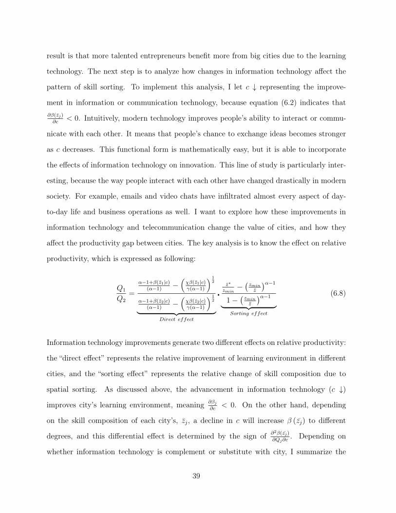
productivity, which is expressed as following:
Q1
Q2=
↵�1+�(z1|c)(↵�1) �
⇣��(z1|c)�(↵�1)
⌘ 12
↵�1+�(z2|c)(↵�1) �
⇣��(z2|c)�(↵�1)
⌘ 12
| {z }Direct effect
⇧z⇤
zmin��zminz
�↵�1
1��zminz
�↵�1
| {z }Sorting effect
(6.8)
Information technology improvements generate two different effects on relative productivity:
the “direct effect” represents the relative improvement of learning environment in different
cities, and the “sorting effect” represents the relative change of skill composition due to
spatial sorting. As discussed above, the advancement in information technology (c #)
improves city’s learning environment, meaning @�j@c
< 0. On the other hand, depending
on the skill composition of each city’s, zj, a decline in c will increase � (zj) to different
degrees, and this differential effect is determined by the sign of @2�(zj)@Qj@c
. Depending on
whether information technology is complement or substitute with city, I summarize the
39
effects in two cases. According to Gaspar and Glaeser (1996), when telecommunications
technology improves, there are two opposing effects on cities and face-to-face interactions:
some relationships that used to be face-to-face will be done electronically (an intuitive
substitution effect), and some individuals will choose to make more contacts, many of
which result in face-to-face interactions. In the case of them being complement, Silicon
Valley is a good example. People in Silicon Valley usually only require two things to work,
phone and computer, so they can easily connect electronically. They could have worked
from anywhere, yet they choose to live in the most expensive city in U.S.. It implies that
human interactions are essential, and cannot be replaced by telecommunications.
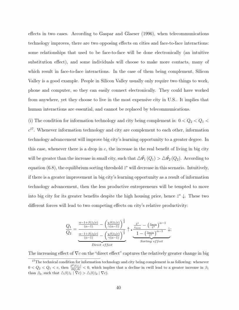
(i) The condition for information technology and city being complement is: 0 < Q2 < Q1 <
c17. Whenever information technology and city are complement to each other, information
technology advancement will improve big city’s learning opportunity to a greater degree. In
this case, whenever there is a drop in c, the increase in the real benefit of living in big city
will be greater than the increase in small city, such that 4 ˜ 1 (Q1) > 4 ˜ 2 (Q2). According to
equation (6.8), the equilibrium sorting threshold z⇤ will decrease in this scenario. Intuitively,
if there is a greater improvement in big city’s learning opportunity as a result of information
technology advancement, then the less productive entrepreneurs will be tempted to move
into big city for its greater benefits despite the high housing price, hence z⇤ #. These two
different forces will lead to two competing effects on city’s relative productivity:
Q1
Q2=
↵�1+�(z1|c)(↵�1) �
⇣��(z1|c)�(↵�1)
⌘ 12
↵�1+�(z2|c)(↵�1) �
⇣��(z2|c)�(↵�1)
⌘ 12
| {z }Direct effect
" ⇧z⇤
zmin��zminz⇤
�↵�1
1��zminz⇤
�↵�1 #| {z }
Sorting effect
;
The increasing effect of rc on the “direct effect” captures the relatively greater change in big17The technical condition for information technology and city being complement is as following: whenever
0 < Q2 < Q1 < c, then @2�(zj)@Qj@c
< 0, which implies that a decline in cwill lead to a greater increase in �1
than �2, such that 4�(z1 | rc) > 4�(z2 | rc).
40
city’s learning environment; the decreasing effect of z⇤ # on the “sorting effect” captures the
negative effect on skill sorting. If the negative sorting effect in part B is the dominant force,
then the equilibrium relative productivity decreases as information technology improves. On
the other hand, if the positive effect in part A is the dominant force, then the equilibrium
relative productivity increases as information technology improves.
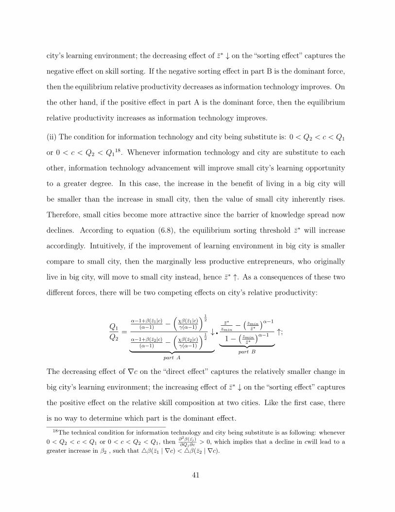
(ii) The condition for information technology and city being substitute is: 0 < Q2 < c < Q1
or 0 < c < Q2 < Q118. Whenever information technology and city are substitute to each
other, information technology advancement will improve small city’s learning opportunity
to a greater degree. In this case, the increase in the benefit of living in a big city will
be smaller than the increase in small city, then the value of small city inherently rises.
Therefore, small cities become more attractive since the barrier of knowledge spread now
declines. According to equation (6.8), the equilibrium sorting threshold z⇤ will increase
accordingly. Intuitively, if the improvement of learning environment in big city is smaller
compare to small city, then the marginally less productive entrepreneurs, who originally
live in big city, will move to small city instead, hence z⇤ ". As a consequences of these two
different forces, there will be two competing effects on city’s relative productivity:
Q1
Q2=
↵�1+�(z1|c)(↵�1) �
⇣��(z1|c)�(↵�1)
⌘ 12
↵�1+�(z2|c)(↵�1) �
⇣��(z2|c)�(↵�1)
⌘ 12
#
| {z }part A
⇧z⇤
zmin��zminz⇤
�↵�1
1��zminz⇤
�↵�1
| {z }part B
";
The decreasing effect of rc on the “direct effect” captures the relatively smaller change in
big city’s learning environment; the increasing effect of z⇤ # on the “sorting effect” captures
the positive effect on the relative skill composition at two cities. Like the first case, there
is no way to determine which part is the dominant effect.18The technical condition for information technology and city being substitute is as following: whenever
0 < Q2 < c < Q1 or 0 < c < Q2 < Q1, then @2�(zj)@Qj@c
> 0, which implies that a decline in cwill lead to agreater increase in �2 , such that 4�(z1 | rc) < 4�(z2 | rc).
41
Now it is time to summarize the above effects. When telecommunication and city are
complementary, the benefits of big cities increased more than that of small cities, because
information technology has made it more and more valuable for people to stay close to
the top talents, thus big cities will attract more and more relatively unskilled people. The
opposite tradeoff occurs when telecommunication and city are substitute. In that case,
the benefits of small cities increased relatively more, because information technology has
rendered it easier for people to learn from top talents over long distance, thus small cities
will attract more and more relatively unskilled people.
Essentially, the effect of localized knowledge exchange provides another perspective as to
why large cities have better environment for idea exchange, without assuming exogenous
differences on locational fundamentals. Therefore, when innovation advantage in large city
is shut down, meaning that �1 = �2, localized knowledge spillover alone still can produce
perfect skill sorting result. The reasoning behind this is that large cities are not only the
places with dense population, they are also the places where the best and brightest minds
live. Knowledge spread is simply faster or more effective when people live close to the ones
that with the best ideas. Just as Marshall (1890) described how in dense concentrations “the
mysteries of the trade become no mystery but are, as it were, in the air.” To simply put,
hanging around successful people will improve the chance of people becoming successful
themselves. Everyone would want to live in the city with best learning opportunities. But
the most talented entrepreneurs are those most able to take advantage of these opportunities
and so most willing to pay for them.
7 Model Extension: Trade
Economic activity depends crucially on the transportation of goods and people across space.
So far the model focuses on the interaction of cities through the mobility of people. This
42
section explores how the input-output linkages affect spatial concentration through includ-
ing bilateral trade into the baseline model. Furthermore, trade and transportation cost
have declined greatly over time. It would be interesting to analyze how the decrease in
trade cost shapes economic activity across space.
Bilateral trade occurs both at the differentiated intermediate goods and final consumption
goods level. Trade cost is assumed to be the typical iceberg form, meaning ⌧nj � 1 units
of must be shipped from city n in order for one unit to arrive in region j. It is neces-
sary to assume asymmetrical trade cost for the purpose of forming asymmetric cities. The
asymmetric trade cost might arise from a number of considerations, such as land gradient
and trade volume (per-unit iceberg trade cost is lower when trade volume is larger). In
addition, big cities, due to scale economy, might provide better or less-costly services re-
lated to trade such as insurance, which then leads to lower ice-berg cost. There are other
plausible channels that capable of generating trade asymmetry. However, it is theoretically
inconsistent to analyze such channels under the framework of this paper. For instance,
Waugh (2010) believed that the asymmetric trade volume is highly correlated with income
level, rather than geographic distance. And it is well known that the consumption baskets
of high and low-income consumers look very different (e.g., Deaton and Muellbauer, 1980).
Fajgelbaum and Khandelwal (2016) suggested that the asymmetry in trade hinges on the
fact that poor consumers spend relatively more on tradable sectors, while high-income in-
dividuals consume relatively more services, which are the least traded sector. Therefore,
trade balance condition will hold because there exists a lower rate of substitution between
imports and domestic goods for the relatively poor. As we can see, the above methods for
modeling asymmetric trade system focus on demand side, and it requires two sectors: trad-
able and non-tradable. But it is conceptually difficult to adopt such extra structure under
this framework. Whereas asymmetric trade cost assumption is a relatively easy approach
in this paper.
43
The production process is the same as the baseline model. In each city there is a final
good producer that supplies the final output good competitively. And final good serves
as numeraire in both cities. Entrepreneurs produce differentiated intermediate goods and
have claims on the net profit. The only difference between baseline model and the extended
model is that the production of final good in a city requires intermediate goods input from
both cities instead of just local varieties. The final good output in city j is defined as
following:
Yj =
0
@X
n2{1,2}
ˆi2⌦
y✓njidi
1
A1/✓
, ✓ 2 (0, 1) (7.1)
where ynji is the amount of intermediate good i (i indexing for entrepreneur) used for
final good production in city j shipped from city n. Profit maximization implies that
intermediate good price is a constant markup over the marginal cost of supplying a variety,
pnji =1
✓
⌧njwn
q�nji. (7.2)
Due to the love of variety, all entrepreneurs sell their differentiated intermediate goods to
both cities. The final output good is numeraire in each city, then the demand of intermediate
good i from city n to city j is
ynji =
✓⌧njwn
✓q�nji
◆ 1✓�1
Yj. (7.3)
Factor market clearing implies that local aggregate output Yj is the sum of imports from
all locations. Replacing (7.3) into final good production function (7.1), the factor market
clearance condition is:
44
"✓✓
wj
◆ 1�
QjYj +
✓✓
⌧njwn
◆ 1�
QnYj
#= Yj. (7.4)
With intermediate goods price function (7.2) and demand function (7.3), the value of
locationj’s imports from location n can be expressed as:
X (n, j) =
ˆpnjiynjidi =
✓✓
⌧njwn
◆ 1�
QnYj. (7.5)
Where Qj still represents the average productivity of entrepreneurs living in city j, and
its definition is Qj =´⌦j
⇣�ji+↵�1↵�1
⌘zjidi. Trade volume expressed in (7.5) states that the
volume of city j’s imports from city n depends on a bilateral trade friction ⌧nj, an origin-
specific cost (inverse) term⇣
✓wn
⌘ 1�Qn, and target market’s size Yj. Goods market clearing
and balanced trade imply that for city n, j 2 {1, 2}, n 6= j :
X (n, j) = X (j, n) .
Replace X (n, j) with (7.5) into the trade balance condition, we can get the following result:
✓✓
⌧12w1
◆ 1�
Q1Y2 =
✓✓
⌧21w2
◆ 1�
Q2Y1. (7.6)
The spatial equilibrium is the same as baseline mode, with an additional condition for
balanced trade. Next I show how the process of innovation and spatial sorting changes.
7.1 Innovation and Skill Sorting
Entrepreneurs face the same choices in the extended trade model. First they decide where
to stay. Then they decide the optimal investment on innovation based on initial skill as well
as the location choice. After which, production takes place. There is no decision needed on
45
whether or not to export, since each and every one of the entrepreneurs will export. Using
equations (7.2) and (7.3), the aggregate profit for entrepreneur i located at city j before
innovation cost is
E�⇡Xji | z
�= (1−✓)
✓✓
wj
◆1/�"Yj +
✓1
⌧jn
◆1/�
Yn
#✓�ji + ↵� 1
↵� 1
◆z. (7.7)
The expected profit in (7.7) indicates that if the cost of shipping goods from two cities are
different, or in this case large city is cost efficient ⌧12 < ⌧21, then choosing which city to
stay has direct effect on the profit from trade. Using the trade balance condition (1.6.6)
and factor market clearance condition (7.4), the expected profit function can be simplified
as
E�⇡Xji | z
�= (1−✓)
Yj
Qj
✓�ji + ↵� 1
↵� 1
◆z. (7.8)
Comparing the expected profit function (4.5) from the baseline model with expression
(7.8), we will notice that they are of the exact same form. This observation indicates the
equilibrium innovation opportunity for each entrepreneur under the two models are exactly
the same. Peculiar as this result may seem, it makes sense mathematically. Because both
the expected profit function and the innovation cost function are linear to city’s economy
size Yj and entrepreneur’s expected productivity qji. This linearity relationship along with
the trade balance condition indicate the equilibrium innovation opportunity �Xji is
�Xji = 1�
✓�j (↵� 1)
�
◆1/2
= �Xj (7.9)
With the expression of expected profit in (7.8) and the optimal innovation opportunity in
(7.9), the expected net profit is
46
⇧Xji (z) = �X
j z. (7.10)
where �Xj =
�↵
(↵�1) � 2
⇣��j
(↵�1)
⌘1/2�wjLj
Qjsummarizes entrepreneur’s return of productivity
for living in city j, which includes the gain from both innovation and trade. With expected
net profit , the skill sorting process is determined by the following utility maximization
problem:
max
j2{1,2}U (z, j) = X
j z � aj. (7.11)
where Xj =
⇣1⌘j
⌘1�µ
�↵(↵�1) � 2
⇣��j
(↵�1)
⌘1/2�(wjLj)
µ
Qjrepresents the real benefit of entrepreneur
living in city j. The process of skill sorting among entrepreneurs is the same before, which
means there exists an unique equilibrium skill threshold zX , such that entrepreneurs with
initial skills higher than zX choosing to live in the big city, and entrepreneurs with initial
skills lower than zX choosing to live in small city. The threshold zX is defined by the
following equation:
zX =
a1 � a2 X1 � X
2
. (7.12)
As proved in appendix A5, when trade cost is asymmetrical, with the large city facing
lower trade cost, skill sorting will become stronger as trade costs decline. For example, if
both city’s ice-berg trade costs decline by the same percentage, say 50%, then the sorting
threshold increases accordingly. Proposition 8 captures this result.
Proposition 8. (Trade Cost Decline and Skill Sorting) With asymmetrical trade costs,
⌧21 > ⌧12, there exists an unique equilibrium with perfect skill sorting: entrepreneur with
initial skill higher than zX choose large city, and entrepreneur with initial skill lower than
47
z⇤ choose small city. In addition, the relative productivity Q1
Q2and relative wage w1
w2across
cities become higher as trade costs decline by the same proportion.
In a economy with asymmetric trade costs, entrepreneurs in large city benefit more from a
trade cost decline, because they end up spending less on shipping goods to the other city,
see equation (7.2). In equilibrium, the benefits of lower trade cost in large city leads to
stronger competition among entrepreneurs. As a result, the relative wage between large
and small city w1w2
increases as trade costs decrease, see detailed proof in appendix A5. In
equilibrium, spatial skill sorting becomes stronger in response to trade cost decline, and the
productivity as well as wage gaps across cities become wider.
8 Conclusions
This paper builds a model to integrate innovation, skill sorting and agglomeration in a
multi-city framework. In the model, innovation and knowledge spillover are the main forces
of agglomeration. The fundamental difference between cities is that some city has better
environment in stimulating innovation, which is reflected as differences in learning opportu-
nities. Everyone would like to be where learning opportunities are the greatest, so that they
can improve productivity. But only the most talented entrepreneurs rise above the compe-
tition, because they are the ones who can afford the higher wages and higher housing prices.
In large cities, entrepreneurs invest more resources to reap the benefits of innovation, hence
innovation activities heavily concentrate in these cities. Meanwhile, the complementarity
between skill sorting and innovation causes the large cities having higher productivity com-
paring to small cities. The productivity premium in large city then leads to higher wages.
48
In equilibrium, the higher nominal wages compensate the higher living costs in big cities.
This paper focus on the interaction between innovation concentration, skill concentration,
and their effects on spacial inequality. Cities play an active role in this framework. A few
city-specific factors serve as channels for spatial skill sorting, such as innovation advantage,
housing supply, and congestion amenity. Through comparative static analysis, we can get
some insights on what are the driving forces behind the increased skill sorting over the past
three decades. In addition, the paper provides a theory on how TFP growth and trade cost
decline affect the distribution of human capital across cities. Over all, this framework prove
to be tractable enough to explore what is causing the great divergence among American
cities.
Furthermore, the extended model in section 6 discussed the effects of localized knowledge
spillover. Spatial knowledge spillover has long been perceived as one of the most important
causes for urban agglomeration. Many theories have proved that sharing knowledge or skill
through social interaction can generate significant spillover effect, which is considered as
the key to economic growth. The emphasis of this paper is to provide a simple theory
of how localized knowledge spillover affects the geographical divergence across cities. In
larger cities, the environment of idea exchange of knowledge spread is better, because they
are the places where the most talented individuals live. And every one wants to hang
out with the smart or successful people, since it gives them the best chances to improve
productivities and enhance innovations. Thus the most skilled and most expensive cities
attract more talented individuals, and become more skill-intensive. This will ultimately
lead the American cities on a diverging trend. And the fact has proved this point. Cities
like New York, San Francisco and Seattle are not bogged down by high living costs, they
are in fact on the rise compared to the rest of cities.
49
References
Aghion, Philippe., Ufuk Akcigit, Antonin Bergeaud, Richard Blundell, andDavid Hemous, “Innovation and Top Income Inequality,” NBER, 2017. Working Paper21247.
Akcigit, Ufuk, John Grigsby, and Tom Nicholas, “The Rise of American Ingenuity:Innovation and Inventors of the Golden Age,” NBER, 2017. Working Paper No. 23047.
Allen, Treb and Costas Arkolakis, “Trade and the Topography of the Spatial Economy,”Quarterly Journal of Economics, 2014, 129, 1085–1140.
Arthur, W.B., Increasing Returns and Path Dependence in the Economy, University ofMichigan Press, 1994.
Bacolod, Marigee, Bernardo S. Blum, and William C. Strange, “Skills in the City,”Journal of Urban Economics, 2009, 65, 136–153.
Baldwin, R.E. and T. Okubo, “Heterogeneous Firms, Agglomeration and EconomicGeography: Spatial Selection and Sorting.,” Journal of Economic Geography, 2006, 6,323–346.
Banerjee, Abhijit, Xin Meng, and Nancy Qian, “The Life Cycle Model and HouseholdSavings: Micro Evidence from Urban China,” 2010. Working paper.
Barth, James R., Michael Lea, and Tong Li, “China’s housing market: Is a bubbleabout to burst?,” Milken Institute, 2012.
Baum-Snow, N. and Ronni Pavan, “Inequality and City Size,” Review of Economicsand Statistics, 2013, 95, 1535–1548.
Behrens, K., G. Mion, Y. Murata, and J. Suedekum, “Trade, Wages, and Produc-tivity,” International Economic Review, 2014, 55, 1305–1348.
Behrens, Kristian and Frederic Robert-Nicoud, “Survival of the Fittest in Cities:Urbanisation and Inequality,” The Economic Journal, 2014, 124, 1371–1400.
, Gilles Duranton, and Frederic Robert-Nicoud, “Productive Cities: Sorting, Se-lection, and Agglomeration,” Journal of Political Economy, 2014, 122.
50
Bleakley, H. and J. Lin, “Portage and Path Dependence,” Quarterly Journal of Eco-nomics, 2012, 127, 587–644.
Buzard, K. and G. Carlino, The Geography of Research and Development Activity inthe U.S. 2013.
Carlino, Gerald and William R. Kerr, “Agglomeration and Innovation,” NBER, 2014.Working Paper No. 20367.
Carroll, Christopher D., “Buffer-Stock Saving and the Life Cycle/Permanent IncomeHypothesis,” Quarterly Journal of Economics, 1997, 112 (1), 1–56.
Chamon, Macros and Eswar Prasad, “Why Are Saving Rates of Urban Households inChina Rising,” American Economic Journal: Macroeconomics, 2010, 2 (1), 93–130.
Chatterji, A., E. Glaeser, and W. Kerr, “Clusters of Entrepreneurship and Innovation,”NBER, 2014. Working Paper No. w19013.
Chen, H., P. Gompers, A. Kovner, and J. Lerner, “Buy Local? The Geography ofVenture Capital,” Journal of Urban Economics, 2010, 67, 90–102.
Chen, Kaiji, Ayse Imrohoroglu, and Selahattin Imrohoroglu, “The Japanese SavingRate,” The American Economic Review, 2006, 96, 1850–1858.
Choukhmane, Taha, Nicolas Coeurdacier, and Keyu Jin, “The One-Child Policyand Household Savings,” Mimeo, Science Po., 2013.
Combes, Pierre-Philippe, Gilles Duranton, and Laurent Gobillon, “Spatial wagedisparities: Sorting matters!,” Journal of Urban Economics, 2008, 63, 723–742.
, , and , “The Costs of Agglomeration: House and Land Prices in French Cities,”2016. Working paper.
Curtis, Chadwick C., Steven Lugauer, and Nelson C. Mark, “Demographic Patternsand Household Saving in China,” American Economic Journal: Macroeconomics, 2015,7 (2), 58–94.
Davis, Donald R. and Jonathan I. Dingel, “A Spatial Knowledge Economy,” NBER,2016. Working Paper.
51
Davis, Morris A. and Francois Ortalo-Magne, “Household Expenditures, Wages,Rents,” Review of Economic Dy namics, 2011, 14, 248–261.
and Stijn Van Nieuwerburgh, “Housing, Finance and the Macroeconomy,” NBER,2014. Working Paper No. 20287.
Deaton, A. and J. Muellbauer, Economics and Consumer Behavior, Cambridge Uni-versity Press, 1980.
Deaton, Angus and Christina H. Paxson, “Growth and Saving among Individuals andHouseholds,” Review of Economics and Statistics, 2000, 82 (2), 212–225.
Desmet, K. and E. Rossi-Hansberg, “Urban Accounting and Welfare,” American Eco-nomic Review, 2013, 103, 2296–2327.
and , “Spatial Development,” American Economic Review, 2014, 104, 1211–1243.
and J.V. Henderson, The Geography of Development within Countries, Vol. 5,
Diamond, R., “The Determinants and Welfare Implications of US Workers’ DivergingLocation Choices by Skill: 1980-2000,” American Economic Review, 2016, 106, 479–524.
Duranton, G., “Urban Evolutions: the Fast, the Slow, and the Still,” American EconomicReview, 2007, 97, 197–221.
and D. Puga, Micro-foundations of Urban Agglomeration Economies, Vol. 4,
Duranton, Gilles, J. Vernon Henderson, and William C. Strange, Handbook ofRegional & Urban Economics, Vol. 5 2015.
Eeckhout, Jan, Roberto Pinheiro, and Kurt Schmidheiny, “Spatial Sorting,” Jour-nal of Political Economy, 2014, 122, 554–620.
Esteve, Albert and Chia Liu, “Families in Asia: A Cross-National Comparison of In-tergenerational Coresidence,” 2013.
Fajgelbaum, Pablo D. and Amit K. Khandelwal, “Measuring the Unequal Gains fromTrade,” Quarterly Journal of Economics, 2016, 131, 1113–1180.
Fang, Hanming, Quanlin Gu, Wei Xiong, and Li-An Zhou, “Demystifying theChinese Housing Boom,” NBER, 2016. Working Paper.
52
Feldman, M. and D. Audretsch, “Innovation in Cities: Science-based Diversity, Spe-cialization, and Localized Competition,” European Economic Review, 1999, 43, 409–429.
Gabaix, Xavier, Jean-Michel Lasry, Pierre-Louis Lions, and Benjamin Moll,“The Dynamics of Inequality,” Econometrica, 2016, 84 (6), 2071–2111.
Gale, William G. and John Karl Scholz, “Intergenerational Transfers and the Accu-mulation of Wealth,” Journal of Economic Perspectives, 1994, 8 (4), 145–160.
Ganong, Peter and Daniel Shoag, “Why has Regional Income Convergence in the U.S.Declined?,” Journal of Urban Economics, 2016. Working Paper.
Gaspar, Jess and Edward Glaeser, “Information Technology and the Future of Cities,”NBER, 1996. Working Paper.
Gennaioli, N., R. La Porta, F. Lopez de Silanes, and A. Shleifer, “Human Capitaland Regional Development,” Quarterly Journal of Economics, 2013, 128, 105–164.
Giannone, Elisa, “Skilled-Biased Technical Change and Regional Convergence,” 2017.Working Paper.
Glaeser, Edward, The Triumph of the City, Penguin Books, 2011.
and Bryce Ward, “The Causes and Consequences of Land Use Regulation: Evidencefrom Greater Boston,” Journal of Urban Economics, 2009, 65, 265–278.
and Joshua D. Gottlieb, “The Wealth of Cities: Agglomeration Economies and SpatialEquilibrium in the United States,” Journal of Economic Literature, 2009, 47, 983–1028.
, Matt Resseger, and Kristina Tobio, “Inequality in Cities,” Journal of RegionalScience, 2009, 49, 617–646.
Goldin, Claudia and Lawrence F. Katz, “Long-Run Changes in the Wage Structure:Narrowing, Widening, Polarizing,” Brookings Papers on Economic Activity, 2007, (2),135–65.
Grossman, G.M., “Heterogeneous Workers and International Trade,” Review of WorldEconomics, 2013, 149, 211–245.
Gyourko, Joseph, Christopher Mayer, and Todd Sinai, “Superstar Cities,” AmericanEconomic Journal: Economic Policy, 2013, 5, 167–99.
53
Henderson, J Vernon, “The Sizes and Types of Cities,” American Economic Review,1974, 64, 640–56.
Henderson, Vernon, Tim Squires, Adam Storeygard, and David Weil, “The GlobalDistribution of Economic Activity: Nature, History, and the Role of Trade,” QuarterlyJournal of Economics, 2017. ISSN 0033-5533.
Holmes, Thomas J. and James A. Schmitz, “Competition and Productivity: A Reviewof Evidence,” Annual Reviews of Economics, 2010, 2 (1), 619–642.
Hsieh, Chang-Tai and Enrico Moretti, “Housing Constraints and Spatial Misalloca-tion,” NBER, 2017. Working Paper No. 21154.
Jones, Charles I. and Jihee Kim, “A Schumpeterian Model of Top Income Inequality,”Journal of Political Economy, 2017. Forthcoming.
Kaplan, Greg, “Moving Back Home: Insurance against Labor Market Risk,” Journal ofPolitical Economy, 2012, 120 (3).
Kerr, W., R. Nanda, and M. Rhodes-Kropf, “Entrepreneurship as Experimentation,”Journal of Economic Perspectives, 2014, 28, 25–48.
la Roca, Jorge De and Diego Puga, “Learning by Working in Big Cities,” Review ofEconomic Studies, 2017, 84, 106–142.
Lee, J. and T. Nicholas, The Origins and Development of Silicon Valley, Harvard Busi-ness School Case, 2013.
Li, Bingqin and Hyun Bang Shin, “Intergenerational Housing Support between RetiredOld Parents and their Children in Urban China,” Urban Studies, 2013, 50 (16), 3325–3242.
Lucas, Robert E., “Externalities and Cities,” Review of Economic Dynamics, 2001, 4,245–274.
and Benjamin Moll, “Knowledge Growth and the Allocation of Time,” Journal ofPolitical Economy, 2014, 122, 1–51.
Manacorda, Marco and Enrico Moretti, “Why do most Italian youths live with theirparents? Intergenerational transfers and household structure,” Journal of the EuropeanEconomic Association, 2006, 4 (4), 800–829.
54
Melitz, M.J., “The Impact of Trade on Intra-industry Reallocations and Aggregate In-dustry Productivity,” Econometrica, 2003, 71, 1695–1725.
Modigliani, Franco and Shi Larry Cao, “The Chinese Saving Puzzle and the Life-CycleHypothesis,” Journal of Economic Literature, 2004, 42 (1), 145–170.
Moretti, Enrico, Human Capital Externalities in Cities 2004.
, The New Geography of Jobs, Houghton Mifflin Harcourt, 2012.
Perla, Jesse and Christopher Tonetti, “Equilibrium Imitation and Growth,” Journalof Political Economy,, 2014, 122 (1), 52–76.
, , and Michael E. Waugh, “Equilibrium Technology Diffusion, Trade, and Growth,”NBER, 2016. Working paper.
Petersen, M. and R. Rajan, “The Benefits of Lending Relationships: Evidence fromSmall Business Data,” J. Finance, 1994, 49, 3–37.
Redding, Stephen J., “Goods Trade, Factor Mobility and Welfare,” Journal of Interna-tional Economics, 2016a, 101, 148–167.
and Esteban Rossi-Hansberg, “Quantitative Spatial Economics,” NBER, 2016b.Working Paper No. 22655.
Rosenzweig, Mark and Junsen Zhang, “Co-residence, Life-Cycle Savings and Inter-generational Support in Urban China,” NBER, 2014. Working Paper.
Ruggles, Steven and Misty Heggeness, “Intergenerational Coresidence in Devel- opingCountries,” Population and Development Review, 2008, 34 (2), 253–281.
Simonovska, Ina and Michael Waugh, “The Elasticity of Trade: Estimates and Evi-dence,” Journal of International Economics, 2014, 92, 34–50.
Song, Zheng and Dennis Tao Yang, “Life Cycle Earnings and Saving in a Fast-GrowingEconomy,” 2012. Working Paper.
Tonetti, Christopher and Jesse Perla, “Equilibrium Imitation and Growth,” Journalof Applied Economics, 2014, 18, 122–148.
Wang, Shing-Yi, “State Misallocation and Housing Prices: Theory and Evidence fromChina,” American Economic Review, 2011, 101 (5), 2081–2107.
55
Waugh, Michael E., “International Trade and Income Differences,” American EconomicReview, 2010, 100, 2093–2124.
Wei, Shang-Jin and Xiaobo Zhang, “The Competitive Saving Motive: Evidence fromRising Sex Ratios and Savings Rates in China,” Journal of Political Economy, 2011, 119(3), 511–564.
Wu, Jing, Joseph Gyourko, and Youngheng Deng, “Evaluating Conditions in MajorChinese Housing Markets,” NBER, 2010. Working Paper.
56
A Mathematical Appendix
APPENDIX A1
Proof of proposition 1: I begin by solving the final goods sector’s problem. Since the
final good is perfectly competitive and its price is normalized to 1, given the price pji of
intermediate good i in city j, the following problem solves for the demand of intermediate
good i :
max
yji
ˆi2⌦j
y✓jidi
!1/✓
�ˆi2⌦j
pjiyjidi;
The demand equations of variety i derived from first order conditions are
pji =
✓Yj
yji
◆1�✓
. (A.1)
According to the intermediate goods production function (3.3), the marginal cost of in-
termediate goods production is wj
q�ji, then profit maximization yields the optimal pricing
rule
pji =1
✓
wj
q�ji, (A.2)
where 1✓
equals the mark-up factor. Together with (A.1) an (A.2), the intermediate good
output yji is
yji =
✓wj
✓q�ji
◆ 1✓�1
Yj. (A.3)
57
Replacing yji =
⇣wj
✓q�ji
⌘1/(✓�1)
Yj into final good production function (3.3), the wage rate of
city j is:
wj = ✓Q�j (A.4)
This expression implies that the equilibrium wage increases with city-specific productivity,
thus the city with more skilled entrepreneurs and more intensive innovation activities has a
higher wage. Rewriting the intermediate good demand function (A.3) with wage equation
(A.4), the output of intermediate good is
yji =
✓qjiQj
◆1/✓
Yj. (A.5)
Combine final good production function and (A.5), together with the labor market clearing
condition Lj =´i2⌦j
ljidi, the aggregate output in city j is
Yj = Q�jLj. (A.6)
Now it is time to solve for entrepreneur’s profit function. Taking advantage of (A.2), (A.3)
, (A.4) and (4.6), the expected profit from selling variety for entrepreneur i in city j is:
E (⇡ji | z) =1� ✓
✓
wj
q�ji
✓wj
✓q�ji
◆ 1✓�1
Yj = (1−✓)Yjz
Qj
✓�ji + ↵� 1
↵� 1
◆. (A.7)
Hence proposition 1 is proved.
58
APPENDIX A2
Proof of proposition 2: Suppose when an entrepreneur’s productivity level is equal to z ,
his indirect utility from living in city 1 and city 2 are the same, meaning
1z � a1 = 2z � a2,
For any constant number � > 0, the following equation holds:
�z ( 1 � 2) = � (a1 � a2) .
If � > 1, then there is
�z ( 1 � 2) > (a1 � a2)
) 1 (�z)� a1 > 2 (�z)� a2.
which means when an entrepreneur’s productivity is �z, for any � > 1, his net profit in
city 1 is higher than that of city 2, thus he will choose to locate in the big city. Similarly,
if 0 < � < 1, then for an entrepreneur with productivity of �z, his net profit in city 1 is
smaller than that of city 2, thus he will locate at the small city.
59
APPENDIX A3
Proof of proposition 4: According to section 4, the skill sorting threshold is z =
a1�a2 1(Q1)� 2(Q2)
,
with
j (Qj) =1
⌘j
✓✓
u⇤+ aj
◆ µ1�µ
"�↵
(↵� 1)
� 2
✓��j
(↵� 1)
◆1/2#Q
�µ+µ�11�µ
j = ⇤jQ�µ+µ�1
1�µ
j .
In addition, equation (4.16) suggests that city j0s productivity is an increasing function
of the skill sorting threshold z, such that @Qi(z)@z
> 0. Rewrite the skill sorting threshold
expression:
z =
a1 � a2
⇤1Q�µ+µ�1
1�µ
1 � ⇤2Q�µ+µ�1
1�µ
2
=
1
(Q2 (z))�µ+µ�1
1�µ
a1 � a2
⇤1
⇣Q1
Q2(z)⌘ �µ+µ�1
1�µ � ⇤2
. (A.8)
We know from (4.16) that the relative productivity Q1
Q2is an increasing function of the skill
sorting threshold z:@⇣
Q1Q2
(z)⌘
@z> 0. Then expression (A.8) indicates that threshold z increases
in aggregate distribution’s minimum productivity threshold zmin, such that @z@zmin
> 0. Hence
the relative productivity is also increasing in minimum productivity threshold zmin:
@⇣
Q1
Q2
⌘
@zmin
> 0.
This positive relationship indicates that TFP growth reinforces the skill sorting process,
making the big city relatively more productive than the small city. Nest, I analyze the effects
of locational fundamentals on skill sorting threshold. Since ⇤1 =1⌘1
⇣✓
u⇤+a1
⌘ µ1�µ
�↵
(↵�1) � 2
⇣��1
(↵�1)
⌘1/2�
is decreasing in �1 , ⌘1 and a1, and it is independent in z, then equation (A.8) can generate
60
the following results:
@z
@�1> 0,
@z
@⌘1> 0 and
@z
@a1> 0.
A higher threshold z indicates stronger skill sorting effects, and a higher relative produc-
tivity Q1
Q2accordingly. Meanwhile the city-specific wage rate is an increasing function of
city productivity, see (4.3). Therefore, the relative wage rate between the two cities w1w2
also
rises with the sorting threshold. In summation:
Q1
Q2" and
w1
w2" if �1 " or ⌘1 " or a1 "
Now, let’s examine the change in relative population density L1/H1
L2/H2:
L1/ ¯H1
L2/ ¯H2=
✓w1
w2
◆ µ1�µ
(u⇤+ a2)
11�µ
(u⇤+ a1)
11�µ
. (A.9)
We know an increase in �1 or ⌘1 lead to an increase in w1w2
, then the relative population
density L1/H1
L2/H2also increases with an increase in �1 or ⌘1. But the effect of a1 on L1/H1
L2/H2is
ambiguous.
APPENDIX A4
Proof of proposition 7: According to section 6, the skill sorting threshold is z⇤ = a1�a2 1(Q1)� 2(Q1)
,
with
˜ j (Qj) =�
⌘j
✓✓
u⇤+ aj
◆ µ1�µ
"↵� 1 + �j(↵� 1)
� 2
✓��j
� (↵� 1)
◆ 12
#Q
�µ+µ�11�µ
j .
61
where �j = zjzj+c
stands for the local learning opportunity. For simplicity, let
˜ j (Qj) =˜
⇤jQ�µ+µ�1
1�µ
j .
Then simple algebra indicates that @⇤j
@�j> 0. In addition, equation (6.5) suggests that city
j0s average productivity is an increasing function of the skill sorting threshold z⇤, such that@Qi(z⇤)@z⇤ > 0. Furthermore, the relative productivity Q1
Q2is also an increasing function of the
skill sorting threshold z⇤:@⇣
Q1
Q2(z⇤)
⌘
@z⇤> 0.
Rewrite the skill sorting threshold expression:
z⇤ =a1 � a2
˜
⇤1Q�µ+µ�1
1�µ
1 � ˜
⇤2Q�µ+µ�1
1�µ
2
=
1
Q�µ+µ�1
1�µ
2
a1 � a2
˜
⇤1Q1
Q2
�µ+µ�11�µ � ˜
⇤2
. (A.10)
If information technology and cities are complement, then a drop in c will lead to a greater
improvement in big city’s learning opportunity, such that 4�1 > 4�2. Therefore, there is
4 ˜
⇤1 > 4 ˜
⇤2 in this case, which means the equilibrium skill sorting threshold decreases as
c decreases:
@z⇤
@c> 0.
If information technology and cities are substitute, then a drop in c will lead to a greater
improvement in small city’s learning opportunity, such that 4�1 < 4�2. Therefore, there
is 4 ˜
⇤1 < 4 ˜
⇤2 in this case, which means the equilibrium skill sorting threshold increases
62
as c decreases:
@z⇤
@c< 0.
The above differentiated results suggest that information technology can cause substantial
changes to city’s skill compositions. Because the way people interact with each other as well
as its relationship with geography can be quite important in terms of economic development
and economic activity distribution across space.
Appendix A5
Proof of proposition 8: The goods market clearance condition imply the local aggregate
output Yj is the sum of labor income wjLj , entrepreneurial profit from domestic market
(1−✓)⇣
✓wj
⌘1/�QjYj and export profit (1−✓)
⇣1⌧jn
⌘1/� ⇣✓wj
⌘1/�QjYn, hence we have
(1−✓)✓✓
wj
◆1/�
Qj
"Yj +
✓1
⌧jn
◆1/�
Yn
#+ wjLj = Yj; (A.11)
With factor market clearance condition (8.4), we can establish the relationship between
city-specific wage rate and average city productivity:
⇣wj
✓
⌘ 1�= Qj
"1 +
✓1
⌧jn
◆ 1�(⌧jn)
1� � 1
(⌧nj)1� � 1
#. (A.12)
Then the trade balance condition (8.6), goods market clearance condition (A.9) and the
wage equation (A.10) lead to the following conclusions:
63
wjLj = ✓Yj (A.13)
Y1
Y2=
w1L1
w2L2=
(⌧21)1� � 1
(⌧12)1� � 1
. (A.14)
Assuming asymmetric trade cost ⌧21 > ⌧12, if there is a proportional drop in trade cost
(namely ⌧12 = ⇢⌧12 , ⌧21 = ⇢⌧21 and 0 < ⇢ < 1), then the relative economy size becomes
larger in response to the trade cost decline
ˆY2
ˆY1
=
(⌧21)1� � 1
(⌧12)1� � 1
>(⌧21)
1� � 1
(⌧12)1� � 1
. (A.15)
Due to the positive relationship between wage and productivity described in (A.12), and the
positive link between city size and wage rate presented in (4.12), the relative productivity
can be expressed as:
Q1
Q2=
(⌧12)1�
(⌧21)1�
⌘1 (u
⇤X + a1)
⌘2 (u⇤X + a2)
� 1�
"(⌧21)
1� � 1
(⌧12)1� � 1
# 1�µ� +1
. (A.16)
where u⇤X is the equilibrium common utility of workers under the trade model, such that
w1
p1�µ1j
� a1 =w2
p1�µh2
� a2 = u⇤X . Taking account of (A.15) and (A.16), there is
ˆQ1
ˆQ2
=
(⌧12)1�
(⌧21)1�
⌘1 (u
⇤X + a1)
⌘2 (u⇤X + a2)
� 1�
"(⌧21)
1� � 1
(⌧12)1� � 1
# 1�µ� +1
>Q1
Q2. (A.17)
Therefore, the relative productivity between the large and small city increases as the trade
cost decreases. Since the relative productivity is increasing in the skill sorting threshold
zX , the negative relationship between skill sorting threshold zX and trade cost is thereby
proved. In addition, the equilibrium relative wage rate w1w2
also increases with a decrease in
64
trade costs.
w1
w2=
⌘1 (u⇤X + a1)
⌘2 (u⇤X + a2)
"(⌧21)
1� � 1
(⌧12)1� � 1
#1�µ
. (A.18)
Equation (A.18) indicates that if trade costs decline, the new equilibrium relative wage w1w2
is
w1
w2=
⌘1 (u⇤X + a1)
⌘2 (u⇤X + a2)
"(⌧21)
1� � 1
(⌧12)1� � 1
#1�µ
>w1
w2. (A.19)
The above proof means that when trade costs decline by the same percentage in the two
cities, the sorting threshold increases accordingly, so are the relative productivity and rel-