Unit 2 Power Flow Analysis - SRM Institute of Science and … · The results of power flow analysis...

��

FORMULATION OF POWER FLOW PROBLEM

Power flow analysis is the most fundamental study to be performed in a

power system both during the Planning and Operational phases. It

constitutes the major portion of electric utility. The study is concerned with

the normal steady state operation of power system and involves the

determination of bus voltages and power flows for a given network

configuration and loading condition.

The results of power flow analysis help to know

1 the present status of the power system, required for continuousmonitoring.

2 alternative plans for system expansion to meet the ever increasing demand.

The mathematical formulation of the power flow problem results in a

system of non-linear algebraic equations and hence calls for an

iterative technique for obtaining the solution. Gauss-Seidel method and

Newton Raphson ( N.R.) method are the commonly used to get the power

flow solution.

With reasonable assumptions and approximations, a power system may

be modelled as shown in Fig. 2.1 for purpose of steady state analysis.

��

�

�

�

Static Capacitor

2

22 jQDPD +G

1 11 jQGPG +

11 jQDPD +

�

�

�

�

�

�

4

44 jQDPD +

3

G

33 δ∠V33 jQGPG +

5

G 55 jQGPG +

��

Fig. 2.1 Typical power system network

The model consists of a network in which a number of buses are

interconnected by means of lines which may either transmission lines or

power transformers. The generators and loads are simply characterized

by the complex powers flowing into and out of buses respectively. Each

transmission line is characterized by a lumped impedance and a line

charging capacitance. Static capacitors or reactors may be located at

certain buses either to boost or buck the load-bus voltages at times of certain buses either to boost or buck the load-bus voltages at times of

need.

Thus the Power Flow problem may be stated as follows:

Given the network configuration and the loads at various buses,

determine a schedule of generation so that the bus voltages and hence

line flows remain within security limits.

A more specific statement of the problem will be made subsequently

after taking into consideration the following three observations.

1 For a given load, we can arbitrarily select the schedules of all the

generating buses, except one, to lie within the allowable limits of

the generation. The generation at one of the buses, called as the

slack bus, cannot be specified beforehand since the total generation

should be equal to the total demand plus the transmission losses, should be equal to the total demand plus the transmission losses,

which is not known unless all the bus voltages are determined.

2 Once the complex voltages at all the buses are known, all other

quantities of interest such as line flows, transmission losses and

generation at the buses can easily be determined. Hence the

foremost aim of the power flow problem is to solve for the bus

voltages.

3 It will be convenient to use the Bus Power Specification which is

defined as the difference between the specified generation and load at

a bus. Thus for the kth bus, the bus power specification Sk is given by

Sk = PIk + j QIk

= (PGk + j QGk) - (PDk + j QDk)

= (PGk - PDk) + j (QGk - j QDk) (2.1)

In view of the above three observations Power Flow Problem may be

defined as that of determining the complex voltages at all the buses,

given the network configuration and the bus power specifications at all

the buses except the slack bus.

CLASSIFICATION OF BUSES

There are four quantities associated with each bus. They are PI, QI, �V� and �.

Here PI is the real power injected into the bus

QI is the reactive power injected into the bus

�V� is the magnitude of the bus voltage

� is the phase angle of the bus voltage

Any two of these four may be treated as independent variables ( i.e.

specified ) while the other two may be computed by solving the power

flow equations. Depending on which of the two variables are specified, flow equations. Depending on which of the two variables are specified,

buses are classified into three types. Three types of bus classification

based on practical requirements are shown below.

��

�� ss QI,PI �� ss �,V �� kk QI,PI �� kV �� k� �� mm QI,PI �� mV �� m� ��

��

��

��

? ? ? ? ? ?

Fig. 2.2 Three types of buses

Slack bus

In a power system with N buses, power flow problem is primarily concerned

with determining the 2N bus voltage variables, namely the voltage

magnitude and phase angles. These can be obtained by solving the 2N

power flow equations provided there are 2N power specifications.

However as discussed earlier the real and reactive power injection at the

SLACK BUS cannot be specified beforehand.

This leaves us with no other alternative but to specify two variables �Vs�

and � arbitrarily for the slack bus so that 2( N-1 ) variables can be and �s arbitrarily for the slack bus so that 2( N-1 ) variables can be

solved from 2( N-1 ) known power specifications.

Incidentally, the specification of �Vs� helps us to fix the voltage level of

the system and the specification of �s serves as the phase angle reference

for the system.

Thus for the slack bus, both �V� and � are specified and PI and QI

are to be determined. PI and QI can be computed at the end, when all the �V� s and �s are solved for.

Generator bus

In a generator bus, it is customary to maintain the bus voltage

magnitude at a desired level which can be achieved in practice by

proper reactive power injection. Such buses are termed as Voltage

Controlled Buses or P – V buses. At these buses PI and �V� are specified

and QI and � are to be solved for. and QI and � are to be solved for.

Load bus

The buses where there is no controllable generation are called as Load

Buses or P – Q buses. At the load buses, both PI and QI are specified

and �V� and � are to be solved for.

POWER FLOW SOLUTION USING GAUSS SEIDEL METHOD

Development of power flow model

The power flow model will comprise of a set of simultaneous non-linear

algebraic equations. These equations relate the complex power injection

to complex bus voltages. The solution of this model will yield all the

bus voltages.

There are three types of equations namely

i) Network equations

ii) Bus power equations

iii) Line flow equations

The first two equations are used for the development of power flow

model. The solution of power flow model will yield all the bus voltages.

Once the bus voltages are known, the line and transformer flows can be

determined using the line flow equations.

Network equations

Network equations can be written in a number of alternative forms. Let

us choose the bus frame of reference in admittance form which is most

economical one from the point of view of computer time and memory

requirements.

The equations describing the performance of the network in the bus

admittance form is given by

I = Y V (2.2)

Here I is the bus current vector,

V is the bus voltage vector and

Y is the bus admittance matrix��

In expanded form these equations are

�

��

�

�

��

�

�

N

2

1

I

II

�=

��

�

�

��

�

�

NNN2N1

2N2221

1N1211

YYY

YYYYYY

�

��

�

�

��

�

�

��

�

�

N

2

1

V

VV

� (2.3) ��

�

��

�

�

��

�

�

N

2

1

I

II

�=

��

�

�

��

�

�

NNN2N1

2N2221

1N1211

YYY

YYYYYY

�

��

�

�

��

�

�

��

�

�

N

2

1

V

VV

� (2.3) ��

Typical element of the bus admittance matrix is

Yij = |Yij | ∠�ij = |Yij | cos �ij + j |Yij | sin �ij = Gij + j Bij (2.4)

Voltage at a typical bus i is Voltage at a typical bus i is

Vi = |Vi | ∠�i = |Vi | ( cos �i + j sin �i ) (2.5)

The current injected into the network at bus i is given by

n

N

1nni

nNi22i11ii

VY

VYVYVY

�=

=

+++= ��I��

(2.6)

Bus power equations

In addition to the linear network equations given by eqn. (2.3), bus

power equations should also be satisfied in power flow problem. These

bus power equations introduce non- linearity into the power flow model.

The complex power entering at the thk bus is given by

*kkkk VQjP I=+ ��(2.7)

This power should be the same as the bus power specification. Thus

we have

*=+ *kkkk VQIjPI I=+ ��(2.8)�

��sk

N,1,2,k≠= �

�

Equations (2.6) and (2.8) can be suitably combined to obtain the power

flow model.

The following two methods are used to solve the power flow model.

1. Gauss-Seidel method

2. Newton Raphson method

Gauss-Seidel method

Gauss-Seidel method is used to solve a set of algebraic equations.

Consider

NNNN2N21N1

2N2N222121

1N1N212111

yxaxaxa

yxaxaxayxaxaxa

=+++

=+++=+++

��

��

��

��

��

Specifically

xayxaThus

yxaxaxaxaN

km1m

mkmkkkk

kNkNkkk2k21k1 ��

��

−=

=+++++

�≠=

N,1,2,k

xaya1

xgivesThis m

N

km1m

kmkkk

k

�=��

�

�

��

�

�

−= �≠=

�

Initially, values of N21 x,,x,x � are assumed. Updated values are calculated

using the above equation. In any iteration 1h + , up to ,1km −= values of mxcalculated�in 1h + iteration are used and for 1km += to N , values of

mx calculated in h iteration are used. Thus�

��

��

�−−= � �

−

= +=

++1k

1m

N

1km

hmkm

1hmkmk

kk

1hk xaxay

a1

x ��(2.9)�

Gauss-Seidel method for power flow solution

In this method, first an initial estimate of bus voltages is assumed. By

substituting this estimate in the given set of equations, a second

estimate, better than the first one, is obtained. This process is repeated

and better and better estimates of the solution are obtained until the

difference between two successive estimates becomes lesser than a

prescribed tolerance.

Let us now find the required equations for calculating the bus voltages.

From the network equations, we have

m

N

km1m

kmkkkm

N

1mkmk

NkNkkk2k21k1k

VYVYVYThus

VYVYVYVY

��≠==

+==

+++++=

I

I ��

��

(2.10)

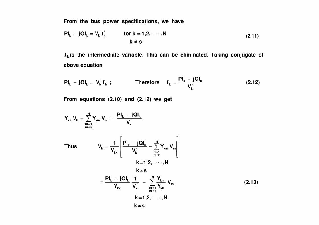
From the bus power specifications, we have

skN,1,2,kfor VQIjPI *

kkkk

≠==+ ��I

��

kI is the intermediate variable. This can be eliminated. Taking conjugate of

above equation�

*k

kkkk

*kkk V

QIjPITherefore;VQIjPI

−==− II ��(2.12)��

From equations (2.10) and (2.12) we get

N QIjPI −

(2.11)

=+ �≠=

m

N

km1m

kmkkk VYVY *k

kk

VQIjPI −

�

skN,1,2,k

VYY

V1

YQIjPI

skN,1,2,k

VYV

jQIPIY1

VThus

m

N

km1m kk

km*

kkk

kk

N

km1m

mkm*k

kk

kkk

≠=

−−

=

≠=

��

�

�

��

�

�

−−

=

�

�

≠=

≠=

��

��

�

(2.13)

A significant reduction in computing time for a solution can be achieved

by performing as many arithmetic operations as possible before initiating

the iterative calculation. Let us define

kkk

kk AY

QIjPI=

−��(2.14)�

kmkk

km BYY

and = ��(2.15)�

Having defined�� kmk BandA ��equation (2.13) becomes�

skN,1,2,kVBVA

VN

km1m

mkm*k

kk ≠=−= �

≠=

�� (2.16)��

When Gauss-Seidel iterative procedure is used, the voltage at the thkbus during th1h + iteration, can be computed as

skN,1,2,k

VBVBVA

VN

1km

hmkm

1k

1m

1hmkm*h

k

k1hk

≠=

−−= ��+=

−

=

++

�� (2.17)�

��

yk0

ikm

ym0

Line flow equations

Knowing the bus voltages, the power in the lines can be computed as

shown below.

�

�

k0kkmmkkm yVy)VV(Current +−=i��(2.18)��

Power flow from bus k to bus m is �

*kmkkm VS i= ��(2.19)�

Fig. 2.3 Circuit for

line flow calculation

ykm

Substituting equation (2.18) in equation (2.19)

]yVy)VV([V S *k0

*k

*km

*m

*kkkm +−= ��(2.20)�

Similarly, power flow from bus m to bus k is

]yVy)VV([V S *m0

*m

*km

*k

*mmmk +−= ��(2.21)

The line loss in the transmission line mk − is given by

mkkmmkL SSS +=− ��(2.22)�

Total transmission loss in the system is �−

−=

linesthealloverji

jiLL SS ��(2.23)

Example 2.1

For a power system, the transmission line impedances and the line charging

admittances in p.u. on a 100 MVA base are given in Table 1. The scheduled

generations and loads on different buses are given in Table 2. Taking the slack

bus voltage as 1.06 + j 0.0 and using a flat start perform the power flow

analysis and obtain the bus voltages, transmission loss and slack bus power.

Table 1 Transmission line data:

Sl. No. Bus code k - m

Line Impedance

kmz HLCA

1 1 – 2 0.02 + j 0.06 j 0.030 2 1 – 3 0.08 + j 0.24 j 0.025 3 2 – 3 0.06 + j 0.18 j 0.020 3 2 – 3 0.06 + j 0.18 j 0.020 4 2 – 4 0.06 + j 0.18 j 0.020 5 2 – 5 0.04 + j 0.12 j 0.015 6 3 – 4 0.01 + j 0.03 j 0.010 7 4 – 5 0.08 + j 0.24 j 0.025

Table 2 Bus data:

�

Bus code k

Generation Load Remark MWinkPG MVARinkQG MWinkPD MVARinkQD

1 --- --- 0 0 Slack bus 2 40 30 20 10 P – Q bus 3 0 0 45 15 P – Q bus 4 0 0 40 5 P – Q bus 5 0 0 60 10 P – Q bus

Solution

Flat start means all the unknown voltage magnitude are taken as 1.0 p.u.

and all unknown voltage phase angles are taken as 0.

Thus initial solution is 0j1.0VVVV

0j1.06V(0)5

(0)4

(0)3

(0)2

1

+====

+=

STEP 1

For the transmission system, the bus admittance matrix is to be calculated.

Sl. No.

Bus code

Line Impedance z

Line admittance y

HLCA No. code

k - m kmz ykm HLCA

1 1 – 2 0.02 + j 0.06 5 - j 15 j 0.030 2 1 – 3 0.08 + j 0.24 1.25 – j 3.75 j 0.025 3 2 – 3 0.06 + j 0.18 1.6667 – j 5 j 0.020 4 2 – 4 0.06 + j 0.18 1.6667 – j 5 j 0.020 5 2 – 5 0.04 + j 0.12 2.5 – j 7.5 j 0.015 6 3 – 4 0.01 + j 0.03 10 – j 30 j 0.010 7 4 – 5 0.08 + j 0.24 1.25 – j 3.75 j 0.025

Y22 = (5 – j15) + (1.6667 – j5) + (1.6667 – j5) + (2.5 – j7.5) + j 0.03 + j 0.02 + j 0.02 + j 0.015

= 10.8334 – j 32.415

Similarly Y33 = 12.9167– j 38.695��Y44 = 12.9167 – j 38.695 ; Y55 = 3.75 – j 11.21

��

��

��

�� !��!��

��!��!��

��

�

STEP 2

Calculation of elements of A vector and B matrix.

0.0037j0.00740.2j0.2QIjPI

A

0.2j0.2QIjPI

0.2j0.2)20j20(100

1QIjPI

YY

BandY

QIjPIA

222

22

22

kk

kmkm

kk

kkk

+=−

−=−

=

−=−

+=+=+

=−

=

manner.similaraincalculatedbecanBmatrixofelementsOther

0.00036j0.4626332.415j10.83345j5

YY

B

.calculatedareAandA,ASimilarly

0.0037j0.007432.415j10.8334Y

A

22

2121

543

222

+−=−+−==

+=−

==

�

Thus

��

��

�� !��!��

��!��

��

��

��"��

��

��

��

�

��

��

��

��

��

��

��

��!�!��

��

��!��

��

�

��

��

��

�

��

��!��

��

��

��

�

��

��!�!��

��

��

��

�

��

��

��

�

��

STEP 3

Iterative computation of bus voltage can be carried out as shown.

New estimate of voltage at bus 2 is calculated as:

)00.0j1.06()0.00036j0.46263(0j1.0

0.00370j0.00740

VBVBVBVBVA

V )0(525

)0(424

)0(323121*)0(

2

2)1(2

++−−−

+=

−−−−=

0.00290j1.03752

)0.0j1.0()0.00018j0.23131()0.0j1.0()0.00012j0.15421()0.0j1.0()0.00012j0.15421(

0j1.0

+=

++−−++−−++−−

−��

This value of voltage V2(1) will replace the previous value of voltage V2

(0)

before doing subsequent calculations of voltages.

This value of voltage V2(1) will replace the previous value of voltage V2

(0)

before doing subsequent calculations of voltages.

The rate of convergence of the iterative process can be increased by

applying an ACCELERATION FACTOR � to the approximate solution

obtained. For example on hand, from the estimate V2(1) we get the

change in voltage

�V2 = V2(1) – V2

(0) = (1.03753 + j 0.00290) – (1.0 + j 0) = 0.03752 + j 0.00290

The accelerated value of the bus voltage is obtained as V2(1) = V2

(0) + � �V2

By assuming � = 1.4 accelerated bus voltage

V2(1) = (1.0 + j 0) + 1.4 (0.03752 + j 0.00290) = 1.05253 + j 0.00406

This new value of voltage V2(1) will replace the previous value of the bus

voltage V2(0) and is used in the calculation of voltages for the remaining

buses. In general

Vkh+1

accld = Vkh + � (Vk

h+1 – Vkh) (2.24)

where k is the bus at which the voltage is calculated and h+1 is the current

iteration count.

The process is continued for the remaining buses to complete one

iteration. For the next bus 3

0.00921j1.00690)0j1.0()0.00033j0.77518(

)0.00406j1.05253()0.00006j0.12920(

)0j1.06()0.00004j0.09690(0j1.00.00930j0.00698

VBVBVBVA

V )0(434

)1(232131*)0(

3

3)1(3

−=++−−

++−−

++−−−−−=

−−−=

�

The accelerated value can be calculated as

V3h+1

accld = V3h + � (V3

h+1 – V3h) = (1.0 + j 0) + 1.4 (0.00690 – j 0.00921) V3

h+1accld = V3

h + � (V3h+1 – V3

h) = (1.0 + j 0) + 1.4 (0.00690 – j 0.00921)

= 1.00966 – j 0.01289

Continuing this process of calculation, at the end of first iteration, the

bus voltages are obtained as

V1 = 1.06 + j 0.0 V2(1) = 1.05253 + j 0.00406 V3

(1) = 1.00966 – j 0.01289

V4(1) = 1.01599 – j 0.02635 V5

(1) = 1.02727 – j 0.07374 ��

If � and � are the acceleration factors for the real and imaginary components

of voltages respectively, the accelerated values can be computed as

ekh+1 = ek

h + � (ekh+1 - ek

h) fkh+1 = fk

h + � (fkh+1 - fk

h) (2.25)

Convergence

The iterative process must be continued until the magnitude of change

of bus voltage between two consecutive iterations is less than a certain

level � for all bus voltages. We express this in mathematical form as

Vmax = max. of |Vkh+1 – Vk

h| �for��k = 1,2, …… , N k s

and Vmax < �

If �1 and �2 are the tolerance level for the real and imaginary parts of

bus voltages respectively, then the convergence criteria will be

(2.26)

�Vmax 1 = max. of ��|ekh+1 – ek

h| ��Vmax 2 = max. of��|fkh+1 – fk

h| ��

for��k = 1,2, …… , N k s

Vmax 1 < �1 and Vmax 2 < �2��

For the problem under study��1 = �2 = 0.0001��

The final converged bus voltages obtained after 10 iterations are given below.

V1 = 1.06 + j 0.0 V2 = 1.04623 - j 0.05126 V3 = 1.02036 – j 0.08917

V4 = 1.01920 – j 0.09504 V5 = 1.01211 – j 0.10904

(2.35) (2.27)

Computation of line flows and transmission loss��

Line flows can be computed from

)0.086j0.888(]})0.03j0.0(0)j1.06({

)15j5(})0.05126j1.04623()0j1.06({[)0j(1.06]yVy)VV([VS

]yVy)VV([VS*10

*1

*12

*2

*1112

*k0

*k

*km

*m

*kkkm

−=−−+

++−−+=+−=

+−=

�

)0.086j0.888( −=

)0.062j0.874(]})0.03j(0.0)0.05126j1.04623({

15)j5}()0j1.06(0.05126)j1.04623({[)0.05126j1.04623(yVy)VV([VS

Similarly*20

*2

*12

*1

*2221

+−=−++

+−−+−=+−=

�

Power loss in line 1 – 2 is

)0.024j0.014(

0.062)j0.874(0.086)j(0.888SSS 211221L

−=

+−+−=+=−�

Power loss in other lines can be computed as

0.029j0.004S

0.033j0.004S

0.019j0.012S

42L

32L

31L

−=

−=

−=

−

−

−

��

0.051j0.0S

0.019j0.0S

0.002j0.011S

0.029j0.004S

54L

43L

52L

42L

−=

−=

+=

−=

−

−

−

−

Total transmission loss SL = ( 0.045 - j 0.173 ) i.e.

Real power transmission loss = 4.5 MW

Reactive power transmission loss = 17.3 MVAR ( Capacitive )

S ds

Computation of slack bus power

Slack bus power can be determined by summing up the powers flowing

out in the lines connected at the slack bus and the load at the slack bus.

��

�

��

��

��

�

S13

S gs

S12

��

��

�

In this case, load at slack bus is zero and hence slack bus power is�

1213gs SSS +=

)0.011j0.407(]})0.025j0.0(0)j1.06({

)3.75j1.25(})0.08917j1.02036()0j1.06({[)0j(1.06]yVy)VV([VS *

10*

1*13

*3

*1113

+=−−+

++−−+=+−=

�

)0.075j1.295( )0.086j0.888()0.011j0.407(SSS 1213gs −=−++=+=

Thus the power supplied by the slack bus:

Real power = 129.5 MW Reactive power = 7.5 MVAR (Capacitive )

Voltage controlled bus

In voltage controlled bus k net real power injection kPI and voltage

magnitude kV are specified. Normally minmax QIandQI will also be

specified for voltage controlled bus. Since kQI is not known, kA given

by kk

kk

YQIjPI −

cannot be calculated. An expression for kQI can be

developed as shown below.

We know�� k*kkk

*kkkkm

N

1mmkk IVQIjPIi.e.IVQIjPIandVY =−=+= �

=I �

Denoting�� havewe�VVand�YY iiijijiji ∠=∠= �

�

��

=

==

−+−=

−+=+∠−∠=−

N

1mkmmkmkmkk

kmmkmk

N

1mmkmmkm

N

1mmkkkkk

��sinYVVQIThus

��YVV��VY�VQIjPI

�

The value of kV to be used in equation (2.28) must satisfy the

relation

specifiedkk VV = �

(2.28)

Because of voltage updating in the previous iteration, the voltage

magnitude of the voltage controlled bus might have been deviated from

the specified value. It has to be pulled back to the specified value,

using the relation

Adjusted voltage� hk

hk

hkh

k

hk1h

khkspecifiedk

hk fjeVtaking)

ef

(tan�where�VV +==∠= −

Using the adjusted voltage hkV as given in eqn. (2.29), net injected

reactive power hkQI can be computed using eqn. (2.28). As long as h

kQI

falls within the range specified, hkV can be replaced by the Adjusted

hV and A can be computed.

(2.29)

hkV and kA can be computed.

In case if hkQI falls beyond the limits specified, h

kV should not be

replaced by Adjusted hkV , h

kQI is set to the limit and kA can be

calculated. In this case bus k is changed from P – V to P – Q type.

Once the value of kA is known, further calculation to find 1hkV + will be

the same as that for P – Q bus.

Complete flow chart for power flow solution using Gauss-Seidel method

is shown in Fig. 2.4. The extra calculation needed for voltage controlled

bus is shown between X – X and Y – Y.

START

READ LINE DATA & BUS DATA FORM Y MATRIX

ASSUME skNkVk ≠= ,,2,1)0(�

COMPUTE kA FOR P – Q BUSES

COMPUTE kmB SET h = 0

SET k = 1 AND 0.0=∆ MAXV

k : s YES

X -------------------------------------------- NO----------------------------------------- NO k : V.C. Bus X YES

COMPUTE hkδ ADJUSTED VOLTAGE, h

kQI

≤ ≥ MAXk

hk QIQI : MINk

hk QIQI :

> <

REPLACE hkQI BY MAXkQI REPLACE h

kQI BY MINkQI REPLACE hkV BY ADJ h

kV kQI MAXkQI kQI MINkQI kV kV Y COMPUTE kA Y

-----------------------------------------------------------------------------------------------------------------

COMPUTE ;1+hkV COMPUTE h

kh

k VVV −=∆ +1

YES MAXVV ∆≥∆ SET VVMAX ∆=∆

NO

REPLACE hkV BY 1+h

kV

SET k = k + 1 k : N IS MAXV∆ <ε YES

NO SET h = h + 1

COMPUTE LINE FLOWS, SLACK BUS POWER PRINT THE RESULTS STOP

≤ >

Introduction

Gauss-Seidel method of solving the power flow has simple problem formulation and

hence easy to explain However, it has poor convergence characteristics. It takes large

number of iterations to converge. Even for the five bus system discussed in Example 2.1,

it takes 10 iterations to converge.

Newton Raphson (N.R.) method of solving power flow is based on the Newton Raphson

method of solving a set of non-linear algebraic equations. N. R. method of solving power

flow problem has very good convergence characteristics. Even for large systems it takes

only two to four iterations to converge. only two to four iterations to converge.

Newton Raphson method of solving a set of non-linear equations

Let the non-linear equations to be solved be

1k)x,,x,(xf n211 =��

2n212 k)x,,x,(xf =��

�

nn21n k)x,,x,(xf =��

�

Let the initial solution be (0)n

(0)2

(0)1 x,,x,x ��

If�� 0)x,,x,(xfk (0)n

(0)2

(0)111 ��− ��

��

��

��

�� 0)x,,x,(xfk (0)n

(0)2

(0)122 −

��

�� 0)x,,x,(xfk (0)n

(0)2

(0)1nn ��− �

then the solution is reached. Let us say that the solution is not reached. Assume

n21 �x,,�x,�x �� are the corrections required on (0)n

(0)2

(0)1 x,,x,x �� respectively.

Then

�

1k)]�x(x ,), �x(x),�x[(x f n(0)n2

(0)21

(0)11 =+++ ��

��

�� 2n(0)n2

(0)21

(0)12 k)]�x(x,),�x(x),�x[(xf =+++

��(2.30)

nn(0)n2

(0)21

(0)1n k)]�x(x ,),�x(x),�x[(xf =+++ ��

Each equation in the above set can be expanded by Taylor’s theorem around(0)n

(0)2

(0)1 x,,x,x �� . For example, the following is obtained for the first equation.

(0)n

(0)2

(0)11 x,,x,(xf ��

1

1

xf

)∂∂

+ 2

11 x

f�x

∂∂

+ n

12 x

f�x

∂∂

++ �� 11n k��x =+

where 1� is a function of higher derivatives of 1f and higher powers of

n21 �x,,�x,�x �� . Neglecting 1� and also following the same for other

equations, we get

f∂ f∂ f∂��

��

��

��

(0)n

(0)2

(0)11 x,,x,(xf ��

1

1

xf

)∂∂

+ ��

2

11 x

f�x

∂∂

+ ��

n

12 x

f�x

∂∂

++ �� 1n k�x = ��

(0)n

(0)2

(0)12 x,,x,(xf ��

1

2

xf

)∂∂

+ ��

2

21 x

f�x

∂∂

+ ��

n

22 x

f�x

∂∂

++ �� 2n k�x = ��

��

(0)n

(0)2

(0)1n x,,x,(xf ��

1

n

xf

)∂∂

+ ��

2

n1 x

f�x

∂∂

+ ��

n

n2 x

f�x

∂∂

++ �� nn k�x = ��

(2.31)

��

��

��

��

�� (2.32)

The matrix form of equations (2.31) is��

�� )x,,x,x(fk�xxf

xf

xf (0)

n(0)2

(0)1111

n

1

2

1

1

1�� −

∂∂

∂∂

∂∂

�

)x,,x,x(fk�xxf

xf

xf (0)

n(0)2

(0)1222

n

2

2

2

1

2�� −

∂∂

∂∂

∂∂

��

��

�

��

��

)x,,x,x(fk�xxf

xf

xf (0)

n(0)2

(0)1nnn

n

n

2

n

1

n�� −

∂∂

∂∂

∂∂

The above equation can be written in a compact form as

)X(FK�X)X(F (0)(0)' −= (2.33)

The above equation can be written in a compact form as

)X(FK�X)X(F (0)(0)' −= (2.33)

This set of linear equations need to be solved for the correction vector

��

�

�

��

�

�

=

n

2

1

�x

�x�x

�X�

)X(FK�X)X(F (0)(0)' −= (2.34)

In eqn.(1.50) )X(F (0)' is called the JACOBIAN MATRIX and the vector

)X(FK (0)− is called the ERROR VECTOR. The Jacobian matrix is also denoted as J.

Solving eqn. (2.34) for �X

�X = [ ] 1)0(' )X(F − [ ])X(FK )(0− (2.35)

Then the improved estimate is

�XXX )0(1)( +=

Generalizing this, for th)1h( + iteration

�XXX )h()1h( +=+ where (2.36) �XXX += where (2.36)

[ ] [ ])X(FK)X(F�X )h(1)h(' −= − (2.37)

i.e. �X is the solution of )X(FK�X)X(F )h()h(' −= (2.38)

Thus the solution procedure to solve K)X(F = is as follows :

(i) Calculate the error vector )X(FK (h)−

If the error vector ≈ zero, convergence is reached; otherwise formulate

)X(FK�X)X(F (h)(h)' −=

(ii) Solve for the correction vector �X (ii) Solve for the correction vector �X

(iii) Update the solution as

�XXX (h)1)(h +=+

Values of the correction vector can also be used to test for convergence.

It is to be noted that Error vector = specified vector – vector of calculated values

Example 2.2

Using Newton-Raphson method, solve for 1x and 2x of the non-linear equations

4 2x sin 1x = - 0.6; 4 22x - 4 2x cos 1x = - 0.3

Choose the initial solution as (0)1x = 0 rad. and (0)

2x = 1. Take the precision index on

error vector as 310− .

Solution

Errors are calculated as Errors are calculated as

- 0.6 – (4 2x sin 1x ) = - 0.6

- 0.3 – (4 22x - 4 2x cos 1x ) = - 0.3

The error vector ��

��

�

−−

0.30.6

is not small.

1x0x

2

1

==

�

1x0x

2

1

==

�

It is noted that 1f = 4 2x sin 1x 2f = 4 22x - 4 2x cos 1x

Jacobian matrix is: J =

��

�

�

��

�

�

∂∂

∂∂

∂∂

∂∂

2

2

1

2

2

1

1

1

xf

xf

xf

xf

= ��

��

�

− 1212

112

xcos4x8xsinx4xsin4xcosx4

Substituting the latest values of state variables 1x = 0 and 2x = 1

J = ��

��

�

4004

; Its inverse is 1J − = ��

��

�

0.25000.25

��

�� 40 �

�� 0.250

Correction vector is calculated as

��

��

�

2

1

x�x�

= ��

��

�

0.25000.25

��

��

�

−−

0.30.6

= ��

��

�

−−

0.0750.150

The state vector is updated as ��

��

�

2

1

xx

= ��

��

�

10

+ ��

��

�

−−

0.0750.150

= ��

��

�−0.9250.150

This completes the first iteration.

Errors are calculated as

- 0.6 – (4 2x sin 1x ) = = - 0.047079

- 0.3 – (4 22x - 4 2x cos 1x ) = - 0.064047

The error vector ��

��

�

−−0.0640470.04709

is not small.

0.925xrad.0.15x

2

1

=−=

�

0.925xrad.0.15x

2

1

=−=

�

Jacobian matrix is: J = ��

��

�

− 1212

112


= ��

��

�

−−3.4449160.5529210.5977533.658453


��

��

�

2

1

x�x�

= ��

��

�

−−3.4449160.5529210.5977533.658453

��

��

�

−−

0.0640470.047079

= ��

��

�

−−

0.0212140.016335

��

0.925xrad.0.15x

2

1

=−=

�

The state vector is updated as

��

��

�

2

1

xx

= ��

��

�−0.9250.150

+ ��

��

�

−−

0.0212140.016335

= ��

��

�−0.9037860.166335

This completes the second iteration.


rad.0.166335x −=

- 0.6 – (4 2x sin 1x ) = = - 0.001444

- 0.3 – (4 22x - 4 2x cos 1x ) = - 0.002068

Still error vector exceeds the precision index.

0.903786xrad.0.166335x

2

1

=−=

�

0.903786xrad.0.166335x

2

1

=−=

�

Jacobian matrix is: J = ��

��

�

− 1212

112


= ��

��

�

−−3.2854950.5985560.6622763.565249


��

��

�

2

1

x�x�

= ��

��

�

−−3.2854950.5985560.6622763.565249

��

��

�

−−

0.0020680.001444

= ��

��

�

−−

0.0007280.000540

The state vector is updated as

0.903786xrad.0.166335x

2

1

=−=

�

��

��

��

�

2

1

xx

= ��

��

�−0.9037860.166335

+ ��

��

�

−−

0.0007280.000540

= ��

��

�−0.9030580.166875


- 0.6 – (4 2x sin 1x ) = = - 0.000002

- 0.3 – (4 22x - 4 2x cos 1x ) = - 0.000002

Errors are less than 10-3.

0.903058xrad.0.166875x

2

1

=−=

�

0.903058xrad.0.166875x

2

1

=−=

�

The final values of 1x and 2x are - 0.166875 rad. and 0.903058 respectively.

The results can be checked by substituting the solution in the original equations:

4 2x sin 1x = - 0.6 4 22x - 4 2x cos 1x = - 0.3

In this example, we have actually solved our first power flow problem by N.R. method.

This is because the two non-linear equations of this example are the power flow model

of the simple system shown in Fig. 2.5 below.

��#�$��

�� 1V 1�∠ �� 2V 2�∠ �

�

�

�

��

Here bus 1 is the slack bus with its voltage 1V 1�∠ = 1.0 00∠ p.u. Further 1x

represents the angle 2� and 2x represents the voltage magnitude 2V at bus 2.

p.u.)0.3j0.6(QP 2d2d +=+ �

��#�$��

%�

��

�&'��( )�*$+�+,+-./�

Power flow model of Newton Raphson method

The equations describing the performance of the network in the bus admittance

form is given by

I = Y V (2.39)

In expanded form these equations are

�

��

�

�

��

�

�

N

2

1

I

II

��

��

�

�

��

�

�

NNN2N1

2N2221

1N1211

YYY

YYYYYY

�

��

�

�

��

��

�

�

��

�

�

N

2

1

V

VV

��(2.40)�

Typical element of the bus admittance matrix is

jiY � jiY ji�∠ � � jiY �0)+� ji� �� jiY �+&1� ji� � �� jiG �� jiB ��(2.41)�

Voltage at a typical bus i is

iV � iV � i�∠ � � iV �2�0)+� i� ��+&1� i� �3��(2.42)�

The current injected into the network at bus i is given by

n

N

1nni

nNi22i11ii

VY

VYVYVYI

�=

=

+++= ��

��(2.43)��

1n =

In addition to the linear network equations given by eqn. (2.40), bus power

equations should also be satisfied in the power flow problem. These bus power

equations introduce non- linearity into the power flow model. The complex power

entering the network at bus i is given by

*iiii IVQjP =+ ��(2.44)�

Bus power equations can be obtained from the above two equations (2.43) and (2.44) by eliminating the intermediate variable iI . From eqn. (2.44)

iIVQjP *iii =− ��

*iV � n

N

1nni VY�

=

�� iV � i�−∠ ��=

N

1nniY � ni�∠ � nV � n�∠ �

�� =

N

1niV � nV � niY �� ni� �� n� �� i� �

Separating the real and imaginary parts, we obtain

N

iP � �=

N

1niV nV niY ��0)+�2 ni� �� n� �� i� 3��(2.45)�

iQ � ��=

N

1niV nV niY ��+&1�2 ni� �� n� �� i� 3��(2.46)

The real and reactive powers obtained from the above two equations are referred as

calculated powers. During the power flow calculations, their values depend on the latest

bus voltages. Finally,these calculated powers should be equal to the specified powers.

Thus the non-linear equations to be solved in power flow analysis are

�=

N

1niV nV niY �0)+�2 ni� �� n� �� i� 3�� iPI ��(2.47)��

��=

N

1niV nV niY �+&1�2 ni� �� n� �� i� 3� � iQI ��(2.48)��

It is to be noted that equation (2.47) can be written for bus i only if real power injection It is to be noted that equation (2.47) can be written for bus i only if real power injection at bus i is specified.

Similarly, equation (2.48) can be written for bus i only if reactive power injection at bus i is specified.

Of the N total number of buses in the power system, let the number of P-Q buses be 1N , P-V buses be 2N . Then 1NNN 21 ++= .

Basic problem is to find the

i) Unknown phase angles � at the 21 NN + number of P-Q & P-V buses and

ii) Unknown voltage magnitudes V at the 1N number of P-Q buses.

Thus total number of unknown variables = 21 NN2 +

We can write 21 NN + real power specification equations (eqn.2.47) and 1N reactive power specification equations (eqn.2.48).

Thus total number of equations = 21 NN2 + .

Therefore Number of equations = Number of variables = 21 NN2 +

Thus in power flow study, we need to solve the equations

�=

N

1niV nV niY �0)+�2 ni� �� n� �� i� 3�� iPI ��(2.49)�

for i = 1, 2, …….., N

i � s

and

��=

N

1niV nV niY ��+&1�2 ni� �� n� �� i� 3� � iQI ��(2.50)�

��for i = 1, 2, …….., N

i � s

i � P – V buses

for the unknown variables iδ i = 1,2,…….., N, i � s and

iV i = 1,2,…....., N, i � s , i � P – V buses

The unknown variables are also called as state variables.

Example 2.3

In a 9 bus system, bus 1 is the slack bus, buses 2,5 and 7 are the P-V buses. List the state variables. Also indicate the specified power injections.

Solution

Buses 3,4,6,8 and 9 are P-Q buses.

9864398765432 VandV,V,V,V,�,�,�,�,�,�,�,� are the state variables.

9864398765432 QIandQI,QI,QI,QI,PI,PI,PI,PI,PI,PI,PI,PI are the specified power injections.

We now concentrate on the application of Newton-Raphson procedure in the power flow studies.

Power flow solution by Newton Raphson method

As discussed earlier, taking the bus voltages and line admittances in polar form, in power flow study we need to solve the non-linear equations

�=

N

1niV nV niY �0)+�2 ni� �� n� �� i� 3�� iPI ��(2.14)��

��N

V V Y ��+&1�2� �� 3� �QI ��(2.15)��=1n

iV nV niY ��+&1�2 ni� �� n� �� i� 3� � iQI ��(2.15)�

Separating the term with in = we get

ii2

i GV ��≠=

N

in1n

iV nV niY �0)+�2 ni� �� n� �� i� 3�� iPI ��(2.16)�

−− ii2

i BV �≠=

N

in1n

iV nV niY +&1�2 ni� �� n� �� i� 3� � iQI ��(2.17)�

In a compact form, the above non-linear equations can be written as

PI)V�,(P = ��(2.18)�

QI)V�,(Q = ��(2.19)�

On linearization, we get

��

��

�=�

�

��

�

��

�

�

��

�

�

∂∂

∂∂

∂∂

∂∂

�Q�P

V��

VQ

�

QVP

�

P

��(2.20)�

��

�� ∂∂ V�

( 4.5.��

−= PI�P 0)/#$-.6��789$.��):�� )V�,(P �0)55.+#)16&1'��-)��-4.�#5.+.1-��+)9$-&)1��

−= QI�Q 0)/#$-.6��789$.��):�� )V�,(Q �0)55.+#)16&1'��-)��-4.�#5.+.1-��+)9$-&)1��

To bring symmetry in the elements of the coefficient matrix, VV�

is taken as

problem variable in place of V� .

Then eqn. (2.20) changes to

��

�

�

��

�

�=

��

�

�

��

�

�

��

�

�

��

�

�

∂∂

∂∂

∂∂

∂∂

�Q

�P

VV�

��

VVQ

�

Q

VVP

�

P

��(2.21)�

In symbolic form, the above equation can be written as

��

�

�

��

�

�

=

��

�

�

��

�

�

��

�

�

��

�

�

�Q

�P

VV�

��

LM

NH

��(2.22)�

�

�4.��/8-5&;��< �� &+��=1)( 1��8+��>�?� "�� /8-5&;��

��@ ��

�4.��6&/.1+&)1+��):��-4.��+$*�/8-5&0.+��( &99��*.��8+��:)99)( +A�

< �� )N(N 21 + ;�� )N(N 21 + ��

� �� )N(N 21 + �;�� 1N �

@ �� 1N ��;�� )N(N 21 + ��816�

�� 1N ��;�� 1N �

where 1N is the number of P-Q buses and 2N is the number of P-V buses.

Consider a 4 bus system having bus 1 as slack bus, buses 2 and 3 as P-Q buses and bus 4 as P-V bus for which real power injections 432 PI&PI,PI and

reactive power injections 32 QI&QI are specified. Noting that

32432 VandV,�,�,� are the problem variables, linear equations that are to be

solved in each iteration will be

�� 32432 VV��

�� 2P �� 33

22

2

2

4

2

3

2

2

2 VVP

VVP

�

P�

P�

P∂∂

∂∂

∂∂

∂∂

∂∂

�� 2�� 2�P ��

�� 3P �� 33

32

2

3

4

3

3

3

2

3 VVP

VVP

�

P�

P�

P∂∂

∂∂

∂∂

∂∂

∂∂

�� 3�� 3�P �

��P ��44444 V

PV

PPPP ∂∂∂∂∂�� P ��(2.23)�� 4P �� 3

3

42

2

4

4

4

3

4

2

4 VVP

VVP

�

P�

P�

P∂∂

∂∂

∂∂

∂∂

∂∂

�� 4�� 4�P ��(2.23)�

�� 2Q ��

2

2

�

�Q∂

��

3

2

�

Q∂∂

��

4

2

�

Q∂∂

�� 22

2 VVQ

∂∂

�� 33

2 VVQ

∂∂

��

2

2

VV�

�� 2�Q �

�� 3Q ��

2

3

�

�Q∂

��

3

3

�

Q∂∂

��

4

3

�

Q∂∂

�� 22

3 VVQ

∂∂

�� 33

3 VVQ

∂∂

��

3

3

VV�

�� 3Q� �

The following is the solution procedure for N.R. method of power flow analysis.

1 Read the line data and bus data; construct the bus admittance matrix.

2 Set k = 0. Assume a starting solution. Usually a FLAT START is assumed

in which all the unknown phase angles are taken as zero and unknown voltage

magnitudes are taken as 1.0 p.u.

3 Compute the mismatch powers i.e. the error vector. If the elements of error

vector are less than the specified tolerance, the problem is solved and hence go

��

vector are less than the specified tolerance, the problem is solved and hence go

to Step 7; otherwise proceed to Step 4.

4 Compute the elements of sub-matrices H, N, M and L. Solve

��

��

�

�

��

�

�

=

��

�

�

��

�

�

��

�

�

��

�

�

�Q

�P

VV�

��

LM

NH

��:)5��

��

�

�

��

�

�

VV�

��

��

=�

��

4 Compute the elements of sub-matrices H, N, M and L. Solve

��

��

�

�

��

�

�

=

��

�

�

��

�

�

��

�

�

��

�

�

�Q

�P

VV�

��

LM

NH

��:)5��

��

�

�

��

�

�

VV�

��

��

5 Update the solution as

=�

5 Update the solution as

��V�

�� V�

��V��

�

6 Set k = k + 1 and go to Step 3.

7 Calculate line flows, transmission loss and slack bus power. Print the

results and STOP.

=��=�

Calculation of elements of Jacobian matrix

We know that the equations that are to be solved are

ii2

i GV +�≠=

N

in1n

iV nV niY cos ( ni� + n� - i� ) = iPI (2.24)

−− 2 BV �N

V V Y sin (� + � - � ) = QI (2.25) −− iii BV �≠=

in1n

iV nV niY sin ( ni� + n� - i� ) = iQI (2.25)

i.e. ii PI)V,(�P = (2.26)

ii QI)V�,(Q = (2.27)

The suffix i should take necessary values.

Jacobian matrix is ��

��

�

LMNH

where

VVQLand

�

QM;VVPN;

�

PH∂∂=

∂∂=

∂∂=

∂∂=

Here

P = 2 GV +�N

V V Y cos (� + � - � ) (2.28) iP = ii2

i GV +�≠=

in1n

iV nV niY cos ( ni� + n� - i� ) (2.28)

iQ = −− ii2

i BV �≠=

N

in1n

iV nV niY sin ( ni� + n� - i� ) (2.29)

Diagonal elements:

i

iii

�

PH

∂∂

= = �≠=

N

in1n

iV nV niY sin ( ni� + n� - i� ) = ii2

ii BVQ −− (2.30)

ii2

iii

iii GV2V

VP

N =∂∂

= + �≠=

N

in1n

iV nV niY cos ( ni� + n� - i� )

= iP + ii2

i GV (2.31) = iP + iii GV (2.31)

i

iii

�

QM

∂∂

= = �≠=

N

in1n

iV nV niY cos ( ni� + n� - i� ) = iP - ii2

i GV (2.32)

ii

iii V

VQ

L∂∂

= = ii2

i BV2− - �≠=

N

in1n

iV nV niY sin ( ni� + n� - i� )

= iQ ii2

i BV− (2.33)

Off-diagonal elements:

We know that

iP = ii2

i GV +�≠=

N

in1n

iV nV niY cos ( ni� + n� - i� ) (2.34)

iQ = −− ii2

i BV �≠=

N

in1n

iV nV niY sin ( ni� + n� - i� ) (2.35)

i YVVP

H −=∂

= sin (� + � - � ) (2.36) jijij

iji YVV

�

PH −=

∂∂

= sin ( ji� + j� - i� ) (2.36)

jj

iji V

VP

N∂∂

= = jiji YVV cos ( ji� + j� - i� ) (2.37)

j

iji

�

QM

∂∂

= = jiji YVV− cos ( ji� + j� - i� ) (2.38)

jj

iji V

VQ

L∂∂= = jiji YVV− sin ( ji� + j� - i� ) (2.39)

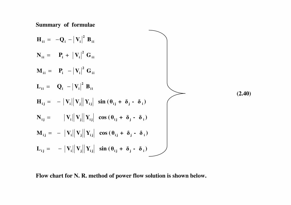
Summary of formulae

=iiH ii2

ii BVQ −−

=iiN iP + ii2

i GV

=iiM iP ii2

i GV−

=iiL iQ ii2

i BV−

=jiH jiji YVV− sin ( ji� + j� - i� ) (2.40)

=jiH jiji YVV− sin ( ji� + j� - i� )

=jiN jiji YVV cos ( ji� + j� - i� )

=jiM jiji YVV− cos ( ji� + j� - i� )

=jiL jiji YVV− sin ( ji� + j� - i� )

Flow chart for N. R. method of power flow solution is shown below.

START

READ LINE and BUS DATA COMPUTE Y MATRIX ASSUME FLAT START

FOR ALL P-V BUSES COMPUTE iQ IF iQ VIOLATES THE LIMITS SET

iQ = LimitiQ AND TREAT BUS i AS A P-Q BUS

COMPUTE MISMATCH POWERS �Q&�P

YES NO

ELEMENTS OF

�Q&�P < � ?

k

COMPUTE MATRICES H,N,M & L

FORM ��

��

�=

��

�

�

��

�

�

��

��

�

�Q�P

VV��

LMNH

; SOLVE FOR ��

�

�

��

�

�

VV��

AND UPDATE

��

��

�

V�

= ��

��

�

V�

+ ��

��

�

V��

SET k = k + 1

COMPUTE LINE FLOWS, TRANSMISSION LOSS & SLACK BUS POWER PRINT THE RESULTS

STOP

k+1 k

�Q&�P < � ?

Example 2.4

Perform power flow analysis for the power system with the data given below, using Newton Raphson method, and obtain the bus voltages.

Line data (p.u. quantities)

0.2j03130.2j03220.1j0211

impedancesLinebusesBetweenNo.Line

+−+−+−

�

Bus data ( p.u. quantities )

Bus

No Type

Generator Load V � minQ maxQ

P Q P Q

1 Slack --- --- 0 0 1.0 0 --- ---

2 P - V 1.8184 --- 0 --- 1.1 --- 0 3.5

3 P - Q 0 0 1.2517 1.2574 --- --- --- ---

�

Solution

The bus admittance matrix can be obtained as

1 2 3 1 2 3

Y = ��

�

�

��

�

�

−−

−

j10j5j5j5j15j10j5j10j15

= j ��

�

�

��

�

�

−−

−

10555151051015

��

��

��

��

��

��

This gives

=Y ��

�

�

��

�

�

10555151051015

and � = ��

�

�

��

�

�

−−

−

000

000

000

909090909090909090

��

��

��

��

��

��

��

��

In this problem

1.2574QI

1.2517PI1.8184PI

3

3

2

−=

−==

and unknown quantities = ��

�

�

��

�

�

3

3

2

V�

�

With flat start 01 01.0V ∠=

02 01.1V ∠=

03 01.0V ∠= 3

We know that

iP = ii2

i GV +�≠=

N

in1n

iV nV niY cos ( ni� + n� - i� )

iQ = −− ii2

i BV �≠=

N

in1n

iV nV niY sin ( ni� + n� - i� )

Substituting the values of bus admittance parameters, expressions for 2P , 3P and 3Qare obtained as follows

2P = )��(cosYVV)��(cosYVVGV 233232322112121222

2

2 −++−++

= 0 + )��90(cosVV5)��90(cosVV10 23322112 −++−+

= )��(sinVV5)��(sinVV10 23322112 −−−−

Similarly Similarly

3P = 5− 3V 1V )��(sin 31 − 5− 3V 2V )��(sin 32 −

Likewise

−−= 332

33 BVQ 3V 1V −−+ )��90(sinY 3113 3V 2V )��(90sinY 3223 −+

= 5V10 23 − 3V 1V 5)��(cos 31 −− 3V 2V )��(cos 32 −

To check whether bus 2 will remain as P-V bus, 2Q need to be calculated.

10V15Q 222 −= 2V 1V 5)��(cos 21 −− 2V 3V )��(cos 23 −

= ( 15 x 1.1 x 1.1 ) – ( 10 x 1.1 x 1 x 1 ) – ( 5 x 1.1 x 1 x 1 ) = 1.65

This lies within the Q limits. Thus bus 2 remains as P – V bus.

Since 0,�� 321 === we get 0PP 32 ==

3Q = ( 10 x 1 x 1 ) – ( 5 x 1 x 1 ) – ( 5 x 1 x 1.1 ) = - 0.5

Mismatch powers are: 1.818401.8184PPI�P =−=−= Mismatch powers are: 1.818401.8184PPI�P 222 =−=−=

1.251701.2517PPI�P 333 −=−−=−=

0.75740.51.2574QQI�Q 333 −=+−=−=

333332

333332

232322

332

LMM

NHHNHHV��

3

3

3

2

VV��

��

=

3

3

2

�Q�P�P

2P �

3P �

3Q �

&1.85�.B$8-&)1+��

-)�*.�+)97.6�85.�

ii2

iiii

iiiiii

ii2

iiii

BVQL

PM;PN

BVQH

−=

==

−−=�

)��(sinYVVM

)��(sinYVVN

)��(cosYVVH

ijjijiji

ijjijiji

ijjijiji

−=

−−=

−−=�

For this problem, since iiG are zero and ji� are 090

=−−= 222

2222 BVQH - 1.65 + ( 1.1 x 1.1 x 15 ) = 16.5

10.5100.5BVQH 332

3333 =+=−−=

0PM;0PN 333333 ====

9.5100.5BVQL 332

3333 =+−=−=

−=32H 2V 3V )��(cosY 2332 − = 5.51x5x1x1.1 −=− and 23H = 5.5−

−=32N 2V 3V 0)��(sinY 2332 =−

=32M 3V 2V 0)��(sinY 3223 =−

Thus ��

�

�

��

�

�

−−

9.500010.55.505.516.5

3

3

3

2

VV��

��

= ��

�

�

��

�

�

−−

0.75741.2517

1.8184

Solving the above

3

3

3

2

VV��

��

= ��

�

�

��

�

�

−−

0.07970.07449

0.08538

Therefore

==+= 0)1(2 4.89rad.0.085380.085380� ==+=

0)1(3 4.27rad.0.074490.074490� −=−=−=

0.92030.07971.0V )1(3 =−=

Thus 01 01.0V ∠=

02 4.891.1V ∠=

03 4.270.9203V −∠=

This completes the first iteration.

Second iteration:

=2Q (15 x 1.1 x 1.1) - (10 x 1.1 x 1.0 cos 04.89 ) - (5 x 1.1 x 0.9203 cos 09.16 )

= 2.1929

This is within the limits. Bus 2 remains as P-V bus.

=2P (10 x 1.1 x 1.0 sin 04.89 ) + ( 5 x 1.1 x 0.9203 sin 09.16 ) = 1.7435

= 0 0=3P - ( 5 x 0.9203 x 1.0 sin 4.27 0 ) – ( 5 x 0.9203 x 1.1 sin 9.16 0 ) = -1.1484

3Q = 10 x 0.9203 x 0.9203 - ( 5 x 0.9203 x 1.0 cos 4.27 0 ) - ( 5 x 0.9203 x 1.1 cos 9.16 0 )

= - 1.1163

=2�P 1.8184 – 1.7435 = 0.0749

=3�P - 1.2517 + 1.1484 = - 0.1033

=3�Q - 1.2574 + 1.1163 = -0.1444

=22H - 2.1929 + ( 1.1 x 1.1 x 15 ) = 15.9571

=33H 1.1163 + (0.9203 x 0.9203 x 10) = 9.5858

33N = - 1.1484; 33M = - 1.1484

=33L - 1.1163 + ( 0.9203 2 x 10 ) = 7.3532

=23H - 1.1 x 0.9203 x 5 cos 9.16 0 = - 4.9971

32H = - 4.9971

=N 1.1 x 0.9203 x 5 sin 9.16 0 = 0.8058 =23N 1.1 x 0.9203 x 5 sin 9.16 0 = 0.8058

32M = 0.8058

The linear equations are

��

�

�

��

�

�

−−−

−

7.35321.14840.80581.14849.58584.9971

0.80584.997115.9571

��

�

�

��

�

�

3

3

3

2

VV��

��

= ��

�

�

��

�

�

−−

0.14440.1033

0.0749

Its solution is

��

�

�

��

�

�

3

3

3

2

VV��

��

= ��

�

�

��

�

�

−−

0.0217820.012388

0.001914

=3V� - 0.9203 x 0.02178 = - 0.02

0)2(2 5.00rad.0.087290.0019140.08538� ==+=

0)2(3 4.98rad.0.086880.0123880.07449� −=−=−−=

0.90320.020.9232V )2(3 =−=

Thus at the end of second iteration

01 01.0V ∠= 0

2 5.001.1V ∠= 03 4.980.9032V −∠=

Continuing in this manner the final solution can be obtained as

01 01.0V ∠= 0

2 51.1V ∠= 03 50.9V −∠=

Once we know the final bus voltages, if necessary, line flows, transmission loss

and the slack bus power can be calculated as discussed in Gauss Seidel method.

DECOUPLED / FAST DECOUPLED POWER FLOW METHOD

In Newton Raphson method of power flow solution, in each iteration, linear

equations

��

�

�

��

�

�

=

��

�

�

��

�

�

��

�

�

��

�

�

Q

P

VV

�

LM

NH

(2.41)

are to be solved for the correction vector . When the power system has are to be solved for the correction vector . When the power system has

N1 number of P-Q buses and N2 number of P-V buses the size of the

Jacobian matrix is 2N1 + N2 . This will not exceed 2 x ( N-1 ) where N is

the number of buses in the power system under study. Even though

factorization method can be adopted to solve such large size linear

algebraic equations, factorization has to be carried out in each iteration

since the elements of the Jacobian matrix will change in values in each

iteration. This results in enormous amount of calculations in each iteration.

In practice, however, the Jacobian matrix is often recalculated only every

few iterations and this speeds up the overall solution process. The final

solution is obtained, of course, by the allowable power mismatches at

the buses.

When solving large scale power systems, an alternative strategy for

improving computational efficiency and reducing computer storage

requirements, is the FAST DECOUPLED POWER FLOW METHOD, which requirements, is the FAST DECOUPLED POWER FLOW METHOD, which

makes use of an approximate version of the Newton Raphson procedure.

The principle underlying the decoupled approach is based on a few

approximations which are acceptable in large practical power systems.

As a first step, the following two observations can be made:

1 Change in voltage phase angle at a bus primarily affects the flow of

real power in the transmission lines and leaves the flow of the reactive

power relatively unchanged.

2 Change in the voltage magnitude at a bus primarily affects the flow

of reactive power in the transmission lines and leaves the flow of the

real power relatively unchanged.

The first observation states essentially that the elements of the Jacobian

sub-matrix H are much larger than the elements of sub-matrix M, which sub-matrix H are much larger than the elements of sub-matrix M, which

we now consider to be approximately zero.

The second observation means that the elements of sub-matrix L are

much larger than the elements of sub-matrix N which are also

considered to be approximately zero.

Incorporation of these two approximations in equation (2.41) yields two

separated systems of equations

P�H = (2.42)

QVV

L = (2.43)

The above two equations are DECOUPLED in the sense that the voltage

phase angle corrections � are calculated using only real power

mismatches P, while voltage magnitude corrections �V� are calculated

using only Q mismatches. using only Q mismatches.

However, the coefficient matrices H and L are still interdependent

because the elements of matrix H depend on voltage magnitudes, being

solved in eqn. (2.43), whereas the elements of matrix L depend on

voltage phase angles that are computed from eqn. (2.42). Of course, the

two sets of equations could be solved alternately, using in one set the

most recent solution from the other set.

The power flow method that uses the decoupled equations is known as

DECOUPLED POWER FLOW METHOD. But this scheme would still

require evaluation and factorizing of the coefficient matrices at each

iteration. The order of the two equations to be solved will not be more

than N-1. As compared to Newton Raphson method, wherein the order

on equations to be solved will be about 2 x ( N-1), Decoupled Power

Flow method requires less computational effort.

If the coefficient matrices do not change in every iteration, factorization If the coefficient matrices do not change in every iteration, factorization

need to be done only once and this will result in considerable reduction

in the calculations. To achieve this we introduce further simplifications,

which are justified by the physics of transmission line power flow. This

leads to FAST DECOUPLED POWER FLOW METHOD in which the

coefficient matrices become constant matrices. These matrices are

factorized only once. During different iteration, only mismatch powers are

recalculated and the solution is updated easily.

In a well designed and properly operated power transmission system:

1 The differences )��( qp − between two physically connected buses of

the power system are usually so small that

)��(cos qp − )��()��(sinand;1 qpqp −≈−≈ (2.44)

2 The line susceptances Bpq are many times larger than the line

conductances Gpq so that

)��(sinG − << )�(�cosB − (2.45) )��(sinG qppq − << )�(�cosB qppq − (2.45)

3 The reactive power Qp injected into any bus p of the system during

normal operation is much less than the reactive power which would flow

if all lines from that bus were short circuited to reference bus. That is

Qp << pp

2

p BV (2.46)

The above approximations can be used to simplify the elements of

Jacobian sub-matrices H and L.

The diagonal elements of sub-matrices H and L are given in eqns. (2.30) and

(2.33).

Hii = - Qi - �Vi�2 Bii (2.30) Lii = Qi - �Vi�

2 Bii (2.33)

They now become

Hii = Lii = - �Vi�2 Bii (2.47)

The off-diagonal elements of sub-matrices H and L are given in eqns. (2.36)

and (2.39).

Hij = - �Vi� �Vj� �Yij� sin (�ij + �j – �i) (2.36) Hij = - �Vi� �Vj� �Yij� sin (�ij + �j – �i) (2.36)

Lij = - �Vi� �Vj� �Yij� sin (�ij + �j – �i) (2.39)

Knowing that

�Yij� sin (�ij + �j – �i) = �Yij� sin �ij cos (�j – �i) + �Yij� cos �ij sin (�j – �i)

= Bij cos (�j – �i) + Gij sin (�j – �i)

� Bij cos (�j – �i) � Bij

Hij = Lij = - �Vi� �Vj� Bij (2.48)

For a 4 bus system having bus 1 as slack bus, buses 2 and 3 as P-Q

buses and bus 4 as P-V bus the linear equations to be solved in N.R.

are shown in eqn. (64). Incorporating the above two equations, the decoupled

equations become

24422332222

2 BVVBVVBV −−− 2� 2P

3443332

33223 BVVBVBVV −−− 3� = 3P (2.49)

�2 �3 �4

P3

P2

442

443344224 BVBVVBVV −−− 4� 4P

2332222

2 BVVBV −− 2

2

VV

2Q

332

33223 BVBVV −− 3

3

VV

3Q

Q2

Q3

(2.50)

P4

�

|V2| |V3|

Equation (2.49) can be rearranged as

244233222 BVBVBV −−− 2� 2

2

VP

344333322 BVBVBV −−− 3� =

��

��

(2.51)

444433422 BVBVBV −−− 4� 4

4

VP

To make the above coefficient matrix to be independent of bus voltage

P4

P3

P2

�2 �3 �4

magnitude, 32 V,V and 4V are set to 1.0 per unit in the left hand side

expression. Then the above equation becomes

242322 BBB −−− 2� 2

2

VP

343332 BBB −−− 3� = 3

3

VP

(2.52)

444342 BBB −−− 4� 4

4

VP

P4

P3

P2

�2 �3 �4

This can be written in a compact form as

VP

�B' = (2.53)

Now equation (2.50) can be rearranged as

32 VV

BB −− V 2Q Q2 2322 BB −− 2V

2

2

V

3332 BB −− 3V 3

3

VQ

This can be written in a compact form as

VQ

VB" = (2.55)

�� (2.54)

Q2

Q3

In a large power network, the bus admittance matrix is symmetrical and

sparse. Separating the real and imaginary parts, it can be written as

BjGY +=

The constant matrix B’ is obtained from matrix B

(1) deleting the row and column corresponding to the slack bus and

(2) changing the sign of all the elements.

The constant matrix B” is obtained from matrix B’ by deleting the rows

and columns corresponding to all the P-V buses.

One typical solution strategy FDPF solution is to:

1 Read line and bus data.

2 Compute bus admittance matrix and form B’ and B” matrices.

3 Assume flat start.

4 Calculate the initial mismatches V/P for all buses except slack bus

5 Solve eqns. VP

�B' = for � V

6 Update the angles � and use them to calculate mismatches V/Q for

all P-Q buses

7 Solve eqns. VQ

VB" = for V and update the magnitudes V and

return to step 4 to repeat the iteration until all mismatches are within

specified tolerances.

The Fast Decoupled Power Flow method uses the constant matrices B’

and B” that are factorized only once. During different iterations repeat

solution is obtained corresponding to the present mismatch power

vectors VP

and VQ

. Thus tremendous amount of computational

simplifications are achieved in Fast Decoupled Power Flow method and

hence it is ideal for large scale power systems.

B =

Example 2.5

Consider the power system described in Example 2.4. Determine the bus

voltages at the end of second iteration, employing Fast Decoupled

Power Flow method.

Solution

Susceptance matrix of the power network is

515102510151321

−−

B =

10553515102

−−

The constant matrices are

10535152

32

−−

Initial solution is 0

3

02

01

01.0V

01.1V

01.0V

∠=

∠=

∠=

='B � and B” = 10

As in example 2.4, 1.8184P2 = and 1.2517P3 −=

Therefore 1.2517VP

;1.6531VP

3

3

2

2 −==

Thus VP

�B' = yields ��

��

�

−−105

515 �

�

��

�

3

2

�

� = �

�

��

�

− 1.25171.6531

On solving the above

�� 2� = 1

�� 510

�� 1.6531 =

�� 0.08218 �

�

��

�

3

2

�

� =

1251 �

�

��

�

155510

��

��

�

− 1.25171.6531

= ��

��

�

− 0.084080.08218

0)1(2 4.71rad.0.082180.082180� ==+=

0)1(3 4.82rad.0.084080.084080� −=−=−=

This gives 0

3

02

01

4.821.0V

4.711.1V

01.0V

−∠=

∠=

∠=

Reactive power at bus 3 is calculated as

−=3Q [{ 5 x 1.0 x 1.0 cos ( )}4.820− +{ 5 x 1.0 x 1.1 cos ( )}9.530− - ( 10 x 1.0 x 1.0)]

= 0.4064−

0.8510.40641.2574QQIQ 333 −=+−=−=

Thus VQVB" = yields

10 3V = - 0.851 i.e. 3V = - 0.0851

This gives 0.91490.08511.0V )1(3 =−=

At the end of first iteration, bus voltage

03

02

01

4.820.9149V

4.711.1V

01.0V

−∠=

∠=

∠=

Second iteration:

−=2Q {( 10 x 1.1 x 1.0 cos −)4.710 ( 15 x )1.12 + ( 5 x 1.1 x 0.9149 cos )}9.530

= 2.2246

This is within the limits. Bus 2 remains as P-V bus.

=2P ( 10 x 1.1 x 1.0 sin +− 0)4.710 ( 5 x 1.1 x 0.9149 sin )9.530 = 1.7363

=3P { 5 x 0.9149 x 1.0 sin ( )}4.820− + { 5 x 0.9149 x 1.1 sin ( 0)}9.530 −−

= - 1.2175 = - 1.2175

0.08211.73631.8184P2 =−=

0.03421.21751.2517P3 −=+−=

0.03738VP

;0.07464VP

3

3

2

2 −==

Equation with 2� and 3� as variables are ��

��

�

−−105

515 �

�

��

�

3

2

�

� = �

�

��

�

− 0.037380.07464

On solving this ��

��

�

3

2

�

� = �

�

��

�

− 0.00150.004476

0)2(2 4.97rad.0.086660.0044760.08218� ==+=

0)2(3 4.90rad.0.085580.00150.08408� −=−=−−=

This gives 01 01.0V ∠=

02 4.971.1V ∠=

03 4.900.9149V −∠=

Reactive power at bus 3 is calculated as

−=3Q [{ 5 x 0.9149 x 1.0 cos ( )}4.900− +{ 5 x 0.9149 x 1.1 cos ( )}9.870−

(− 10 x 20.9149 )] = 1.1448−

0.1231VQ

;0.11261.14481.2574Q3

33 −=−=+−=

Thus VQ

VB" = yields 10 3V = - 0.1231 i.e. 3V = - 0.01231

This gives 0.90260.012310.9149V )2(3 =−=

At the end of second iteration, bus voltages are

01 01.0V ∠=

02 4.971.1V ∠=

03 4.900.9026V −∠=

Problem Set 2

1. Fig. 2.7 shows the one-line diagram of a simple three-bus power system with

generation at bus 1. The voltage at bus 1 is V1 = 1.0 ∠ 00 per unit.The

scheduled load at buses 2 and 3 are marked on the diagram. Line impedances

are marked in per unit on a 100-MVA base.

j 0.0125

j 0.05

320 Mvar

400 MW

�

V1 = 1∠ 00

Slack

1 2 j 0.03333

(a) Assuming a flat start using Gauss-Seidel method determine V2 and V3.

Perform two iterations. Take acceleration factor as 1.2.

(b) If after several iterations the bus voltages converge to V2 = (0.9 – j 0.1) pu

and V3 = (0.95 – j 0.05) pu determine the line flows, line losses, transmission

loss and the slack bus real and reactive power. Construct a power flow

diagram and show the direction of the line flows.

3

300 MW 270 Mvar

Fig. 2.7 One-line diagram for Problem 1

2. Fig. 2.9 shows the one-line diagram of a simple three-phase power system

with generation at buses 1 and 3. The voltage at bus 1 is V1 = 1.025 ∠ 00 per

unit. Voltage magnitude at bus 3 is fixed at 1.03 pu with a real power

generation of 300 MW. A load consisting of 400 MW and 200 Mvar is taken from

bus 2. Line impedances are marked in per unit on a 100-MVA base.

300 MW

�

V1 = 1.025 ∠ 00

Slack

1 3 j 0.05

�

|V | = 1.03

Assuming a flat start using Gauss-Seidel method determine V2 and V3. Perform

two iterations. Take acceleration factor as 1.0.

j 0.025 j 0.025

Slack

2

400 MW 200 Mvar

|V3| = 1.03


3. Consider the two-bus system shown in Fig. 2.9. Base = 100 MVA. Starting

with flat start, using Newton-Raphson method, obtain the voltage at bus 2 at

the end of first and second iteration.

100 MW Slack bus 1 2

0.12 + j 0.16

50 Mvar

�

V1 = 1.0 00∠

0.12 + j 0.16


4. Consider the power system with the following data. Perform power flow

analysis for the power system with the data given below, using Newton

Raphson method, and obtain the bus voltages at the end of first two

iterations.

0.2j03130.2j03220.1j0211

impedancesLinebusesBetweenNo.Line

+−+−+−


Line data ( p.u. quantities )


Bus

No Type

Generator Load V � minQ maxQ

P Q P Q

1 Slack --- --- 0 0 1.0 0 --- ---

2 P - V 5.3217 --- 0 --- 1.1 --- 0 3.5

3 P - Q 0 0 3.6392 0.5339 --- --- --- ---

5. Redo the Problem 4 using Fast Decoupled Power Flow method.

ANSWERS

1. V2(1) = 0.9232 – j 0.096 V3

(1) = 0.9491 – j 0.0590

V2(2) = 0.8979 – j 0.1034 V3

(2) = 0.9493 – j 0.0487

SL 1-2 = S12 + S21 = j 0.6 MVA i.e. 60 Mvar

SL 1-3 = S13 + S31 = j 0.4 MVA i.e. 40 Mvar

SL 1-3 = S13 + S31 = j 0.4 MVA i.e. 40 Mvar

Transmission loss = SL 1-2 + SL 1-3 + SL 2-3

= j 0.6 + j 0.4 + j 0.1 = j 1.1 pu i.e. 110 Mvar

Slack bus power SL = S12 + S13 = (3 + j 3) + (4 + j 4) Slack bus power SL = S12 + S13 = (3 + j 3) + (4 + j 4)

= (7 + j 7) pu i.e. 700 MW and 700 Mvar

V3= 0.95 - j 0.05

V2= 0.9 - j 0.1 V1= 1 + j 0

- 80 Mvar

- 100 MW

90 Mvar

100 MW

-360 Mvar

- 400 MW 400 Mvar

400 MW

- 240 Mvar

- 300 MW

300 Mvar

300 MW

320 Mvar

400 MW

�

Slack

1

3

2

300 MW 270 Mvar

2. At the end of first iteration

V1 = 1.025 + j 0; V2 = 1.0025 - j 0.05; V3 = 1.02989 + j 0.01521

At the end of second iteration

V1 = 1.025 + j 0; V2 =1.00008 - j 0.0409 ; V3 = 1.02978 + j 0.0216

3. At the end of first iteration V2 = 0.8 ∠ - 5.730

At the end of second iteration |V2| = 0.8 – 0.07736 = 0.7226

�2 = - 0.1- 0.035 = - 0.135

Thus V2 = 0.7226 ∠ - 7.7350

4. At the end of first iteration 4. At the end of first iteration

01 01.0V ∠=

02 14.371.1V ∠=

03 12.330.9964V −∠=

At the end of second iteration

0

2 14.9431.1V ∠= 0

3 14.4560.912V −∠=

5. At the end of first iteration, bus voltage

01 01.0V ∠=

02 13.841.1V ∠= 0

3 13.930.9186V −∠=

At the end of second iteration, bus voltages

01 01.0V ∠= 0

30

2 14.570.9799V14.791.1V −∠=∠=

01 01.0V ∠=

Date post:	12-Apr-2018
Category:	Documents
Upload:	duongdang
View:	214 times
Download:	0 times

Unit 2 Power Flow Analysis - SRM Institute of Science and … · The results of power flow analysis...

Documents